the Creative Commons Attribution 4.0 License.
the Creative Commons Attribution 4.0 License.
 | 27 Feb 2024
A diatom extension to the cGEnIE Earth system model – EcoGEnIE 1.1
Aaron A. Naidoo-Bagwell
Fanny M. Monteiro
Katharine R. Hendry
Scott Burgan
Jamie D. Wilson
Ben A. Ward
Andy Ridgwell
Daniel J. Conley
We extend the ecological component (ECOGEM) of the carbon-centric Grid-Enabled Integrated Earth system model (cGEnIE) to include a diatom functional group. ECOGEM represents plankton community dynamics via a spectrum of ecophysiological traits originally based on size and plankton food web (phyto- and zooplankton; EcoGEnIE 1.0), which we developed here to account for a diatom functional group (EcoGEnIE 1.1). We tuned EcoGEnIE 1.1, exploring a range of ecophysiological parameter values specific to phytoplankton, including diatom growth and survival (18 parameters over 550 runs) to achieve best fits to observations of diatom biogeography and size class distribution as well as to global ocean nutrient and dissolved oxygen distributions. This, in conjunction with a previously developed representation of opal dissolution and an updated representation of the ocean iron cycle in the water column, resulted in an improved distribution of dissolved oxygen in the water column relative to the previous EcoGEnIE 1.0, with global export production (7.4 Gt C yr−1) now closer to previous estimates. Simulated diatom biogeography is characterised by larger size classes dominating at high latitudes, notably in the Southern Ocean, and smaller size classes dominating at lower latitudes. Overall, diatom biological productivity accounts for ∼20 % of global carbon biomass in the model, with diatoms outcompeting other phytoplankton functional groups when dissolved silica is available due to their faster maximum photosynthetic rates and reduced palatability to grazers. Adding a diatom functional group provides the cGEnIE Earth system model with an extended capability to explore ecological dynamics and their influence on ocean biogeochemistry.
- Article
(12171 KB) - Full-text XML
-
Supplement
(1002 KB) - BibTeX
- EndNote


Dissolved silica (dSi) – H4SiO4 (orthosilicic acid) – plays a key role in numerous biogeochemical cycles, particularly in marine environments. Marine silicifiers take up dSi across the cell wall, both via diffusion and silicon transporters, to produce biogenic silica (bSi) (hydrated silica – SiO2⋅nH2O), which is used to build internal and external structures (Moriceau et al., 2019; Maldonado et al., 2019). As well as depleting dSi in their local growth environment, the ecological success of silicifiers impacts the cycling of other essential nutrients, such as nitrogen, phosphate, and dissolved iron through competition with non-silicifiers, and potentially also the cycling of carbon. Today, the dominant marine silicifiers are diatoms – phytoplankton with a protective opal frustule (silica shell) that mitigates grazing loss (Van Tol et al., 2012). Diatoms also exhibit relatively fast growth rates (Banse, 1982), enabling them to potentially out-compete other phytoplankton. As a result, the diatom genera is thought to be responsible for approximately 40 % of global primary production in today's ocean (Field et al., 1998). The different cellular nutrient-to-carbon ratio of diatoms compared with other phytoplankton (O'Donnell et al., 2021), as well as the potential for the dense protective opal frustules to modify the mean depth at which carbon (and nutrients) can be returned to the water column from sinking biogenic material, implies that a complete representation of the ocean's “biological pump” requires that we account for the marine cycle of silica (Wilson et al., 2012). However, the spatio-temporal distribution of diatoms and their ability to dominate an ecosystem depends on a number of both environmental pressures, particularly dSi availability, and underlying key metabolic trade-offs, such as control over frustule size, balancing predation vs. buoyancy, and/or optimising their photosynthetic apparatus in light-intensive areas where excess energy must be dissipated (Hendry et al., 2018; Assmy et al., 2013; Lavaud et al., 2004) Indeed, the large number of different possible combinations of trade-offs and marine environments may be behind the evolution of the estimated 30 000–100 000 current species worldwide (Mann and Vanormelingen, 2013).
One way of representing rates of nutrient (and carbon) uptake from the ocean surface and subsequent export of solid (and dissolved) biogenic matter in models is as a direct function of the ambient environment such as temperature, light, and nutrient availability (Maier-Reimer and Hasselmann, 1987). Such an implicit approach has previously been used in box models (Ridgwell et al., 2002). However, the biogenically induced flux modelling approach is limited, both when tasked with exploring events regarding the evolution of ecosystem complexity, as ecosystems are not resolved (i.e. plankton diversity is not considered), and in respect to the details of seasonal productivity cycles and species successions and “blooms”, as standing biomass becomes a key state variable that creates temporal lags in the response of biological export to changes in the ambient physical and chemical environment. Instead, model approaches have been developed that can resolve biomass dynamics across a broad spectrum of complexities (Kwiatkowski et al., 2014). At one end, simple NPZD (N – dissolved inorganic nitrogen, P – phytoplankton, Z – zooplankton, and D – detritus) models (Kriest et al., 2010) are able to reproduce the variability in the mean ecosystem by simulating the effects of limiting factors (e.g. nutrient limitation), but they fail to constrain potentially important biogeochemical processes and feedbacks associated with the biological pump due to their simplicity (Yool et al., 2013). Beyond this, in terms of complexity, models may include multiple (plankton) functional types (PFTs) to better resolve fundamental biogeochemical functions, including those less sensitive to environmental perturbation (Friedrichs et al., 2007; Quere et al., 2005). However, PFTs are generally based explicitly on the observed characteristics of modern plankton, potentially impacting their prospective application to past climates (Ward et al., 2018; Falkowski et al., 2004). The relationships between species, ecosystems, and the environment continually evolve through time, such as the diversification of diatoms in the Cenozoic and their increasing dominance of dSi uptake (Conley et al., 2017). In turn, this has led to “trait-based” approaches that focus on the governing rules of diversity, as opposed to imposing a specific and restricted diversity, being devised (Follows and Dutkiewicz, 2011; Follows et al., 2007). Besides requiring fewer total parameters to be specified, trait-based approaches allow a greater resolution of diversity. However, they also require the identification of the underlying trade-offs that govern species competition and coexistence (Kiørboe et al., 2018). Currently, allometric relationships are often assumed to regulate these trade-offs, in which physiological and ecological traits can be linked to organism size (e.g. Mullin et al., 1966). Assuming then that these allometric relationships are consistent through time (or at least, rather more conserved than individual species themselves), trait-based approaches should be comparatively independent of the geological period to which they might be applied.
In the case of the Earth system model of intermediate complexity (EMIC) cGEnIE – a global biogeochemical cycles (ocean circulation and primary climate feedbacks) model designed for addressing palaeo-questions (Ridgwell et al., 2007) – Ward et al. (2018) added a trait-based ecosystem, EcoGEnIE, that explicitly accounts for the growth of plankton with traits assigned based on size and function. The palaeo-utility of now being able to simulate potential ecosystem structures (and associated marine biogeochemical cycles) of the past was demonstrated in Wilson et al. (2018). Here, we build on this earlier work and present an update to the EcoGEnIE 1.0 framework by introducing a diatom phytoplankton functional group (including their allometric relationships) and a marine silicon cycle by tuning the model (now named EcoGEnIE 1.1) using Latin hypercube model parameter sampling (Sect. 3). Finally, we evaluate how the results of our model ensemble with diatoms compare with global observations and the previous version of EcoGEnIE (Sects. 4, 5). We start (Sect. 2) by describing the general structure and properties of the cGEnIE Earth system model (e.g. the marine biogeochemical components most relevant to simulating marine ecology), including a summary of the existing ecosystem model component and how this has been extended to include diatoms.
2.1 Ocean (and atmosphere) physics
The underlying climate component in the configuration of cGEnIE used here comprises a 3-D frictional geostrophic ocean model coupled with a 2-D energy moisture balance model (EMBM) and a dynamic–thermodynamic sea-ice model (Marsh et al., 2011). We employ cGEnIE on a 36×36 longitude vs. latitude grid of equal area (equal divisions in longitude and the sine of latitude), with ocean depth resolved across 16 vertical layers that have a progressively increasing thickness, varying from 80.8 m at the surface to a maximum of 765 m at depth. Here, to retain the same traceable representation of global ocean circulation as Cao et al. (2009) which formed the basis for the development of a variety of new biogeochemical cycles in cGEnIE (Crichton et al., 2021; Reinhard et al., 2020; Van De Velde et al., 2021), we also adopted the same modern continental configuration and ocean bathymetry, as well as calibrated parameters controlling ocean, atmosphere, and sea-ice physics, as Cao et al. (2009). This differs from the physics configuration of Ward et al. (2018), who adopted a slightly modified continental configuration and, more importantly, included a representation of mixed-layer physics (Kraus and Turner, 1967). Ecologically, the depth of the mixed layer is critical to calculating mean light penetration and, hence, photosynthetic rates. Thus, we diagnosed the mixed-layer depth everywhere, calculating what the chlorophyll concentration would be if it were mixed evenly across this depth and what the average light level should be across that depth with that level of chlorophyll (following Ward et al., 2018), but we did not enable temperature nor salinity (nor other tracers) to be physically mixed, thereby retaining the same ocean circulation as Cao et al. (2009). Finally, we also prevent photosynthesis under sea ice (in practice, in each grid cell, light availability is scaled by the ice-free fraction), which was not adopted in Ward et al. (2018). We quantify and discuss the separate impacts of changing ocean physics vs. changing ecosystem structure between EcoGEnIE 1.0 and EcoGEnIE 1.1 as well as the effects of contrasting model projections against observations.
2.2 Ocean biogeochemical cycling framework
The BIOGEM code module in cGEnIE provides the framework for ocean–atmosphere biogeochemical cycling, including regulating air–sea gas exchange as well as the transformation and partitioning of biogeochemical tracers within the ocean. As configured here, BIOGEM accounts for the biogeochemical cycling of carbon, phosphate, oxygen, carbon (Ridgwell et al., 2007), and iron (Tagliabue et al., 2016) as well as a previously developed parameterisation of opal dissolution in the water column (Ridgwell et al., 2002 – summarised below and in the Supplement) in order to complete the ocean silicon cycle in conjunction with the new ECOGEM diatom addition.
For the iron cycle, we took the preindustrial (year 1850) dust field of Albani et al. (2016) to provide dissolved iron input at the ocean surface and carried out a brief parameter calibration of the two key iron-controlling parameters – the mean global (flux-weighted) iron solubility and the scaling factor for the scavenging rate of free (non-ligand bound) iron by sinking particulate organic matter in the water column. This was in the form of a 2-D parameter ensemble of iron solubility vs. scavenging rate with the resulting simulated 3-D distribution of total dissolved iron in the ocean (i.e. free iron and ligand-bound iron) statistically contrasted with observations (Tagliabue et al., 2016). For this parameter tuning, we utilised the (non-ecosystem-based) cGEnIE phosphate- and iron-limited marine biogeochemical cycle configuration of Tagliabue et al. (2016) in the same Cao et al. (2009) configuration of ocean circulation as employed here. We then simply adopted the same two parameter values when using the ecosystem model in EcoGEnIE 1.1 (i.e. iron solubility and scavenging rates in the ocean were calibrated prior to and independently of the ecosystem model). The only differences in ocean iron cycling compared with Ward et al. (2018) are then as follows: (1) the iron cycle is now tuned for the Cao et al. (2009) configuration of ocean circulation and (2) the iron cycle is tuned to the more recent dust deposition field of Albani et al. (2016) (rather than Mahowald et al., 1999). In terms of the resulting parameter values, the mean global solubility of dust-delivered iron is now 0.244 % as opposed to 0.201 %, partly to compensate for the overall lower dust fluxes of Albani et al. (2016) vs. Mahowald et al. (1999), and there is a small reduction in the scavenging rate scaling (0.225 vs. 0.344 in Ward et al., 2018).
To complete the ocean silica cycle, opal must dissolve in the water column and at the seafloor, allowing silica to be released back into solution (dSi). The treatment of how sinking biogenic solid silica (bSi) dissolves in the water column follows Ridgwell et al. (2002), who used a simple quasi-empirical scheme that considered the degree of ambient opal under saturation and evaluated it against sediment trap observations. Note that we do not attempt to calculate the fractional preservation of opal in accumulating sediments at the seafloor in this current paper; instead, we impose a simple benthic “closure” term such that all biogenic matter reaching the bottom of the ocean is entirely dissolved in the lowermost ocean grid cell instead of being buried in the sediments – effectively the same common closure term that is used for all of the (e.g. carbon and nutrient) constituents of particulate organic matter as well as of CaCO3 – all of which are returned back into solution at the model seafloor.
2.3 Ecological structure
The ecological component of the cGEnIE model – EcoGEnIE – consists of a highly configurable generic plankton community (Ward et al., 2018) based on a series of functional groups and respective size classes. Originally, EcoGEnIE 1.0 described and evaluated just two functional types, zooplankton and phytoplankton, which were each delineated into eight size classes (Table 1). A mixotroph functional group was also coded but not described nor evaluated in Ward et al. (2018).
For EcoGEnIE 1.1, we implemented an additional diatom functional group, coded as a microphytoplankton that has a dSi nutrient assimilation requirement, lower palatability, and higher maximum photosynthetic rate than existing groups of an equivalent size class (Tréguer et al., 2018; Follows et al., 2007). As well as adding the diatom functional group, we also differentiated the generic phytoplankton in EcoGEnIE 1.0 into two derived phytoplankton functional subtypes – “picoplankton” and “eukaryotes” – differentiated by their respective photosynthetic rate exponent (Table 1) based on the trait-based modelling of Dutkiewicz et al. (2020). As per Dutkiewicz et al. (2020), plankton of equivalent spherical diameter <3 µm exhibit an increase in maximum growth rate with increasing size, whereas anything larger than 3 µm exhibits a progressive decrease in maximum growth rate with further increases in size. Hence, the EcoGEnIE 1.1 plankton community now comprises four functional groups (diatoms, picoplankton, eukaryotes, and zooplankton).
Table 1The four EcoGEnIE 1.1 plankton functional groups and the range of equivalent spherical diameter (ESD) “species” focussed on in this paper compared with those used in EcoGEnIE 1.0.
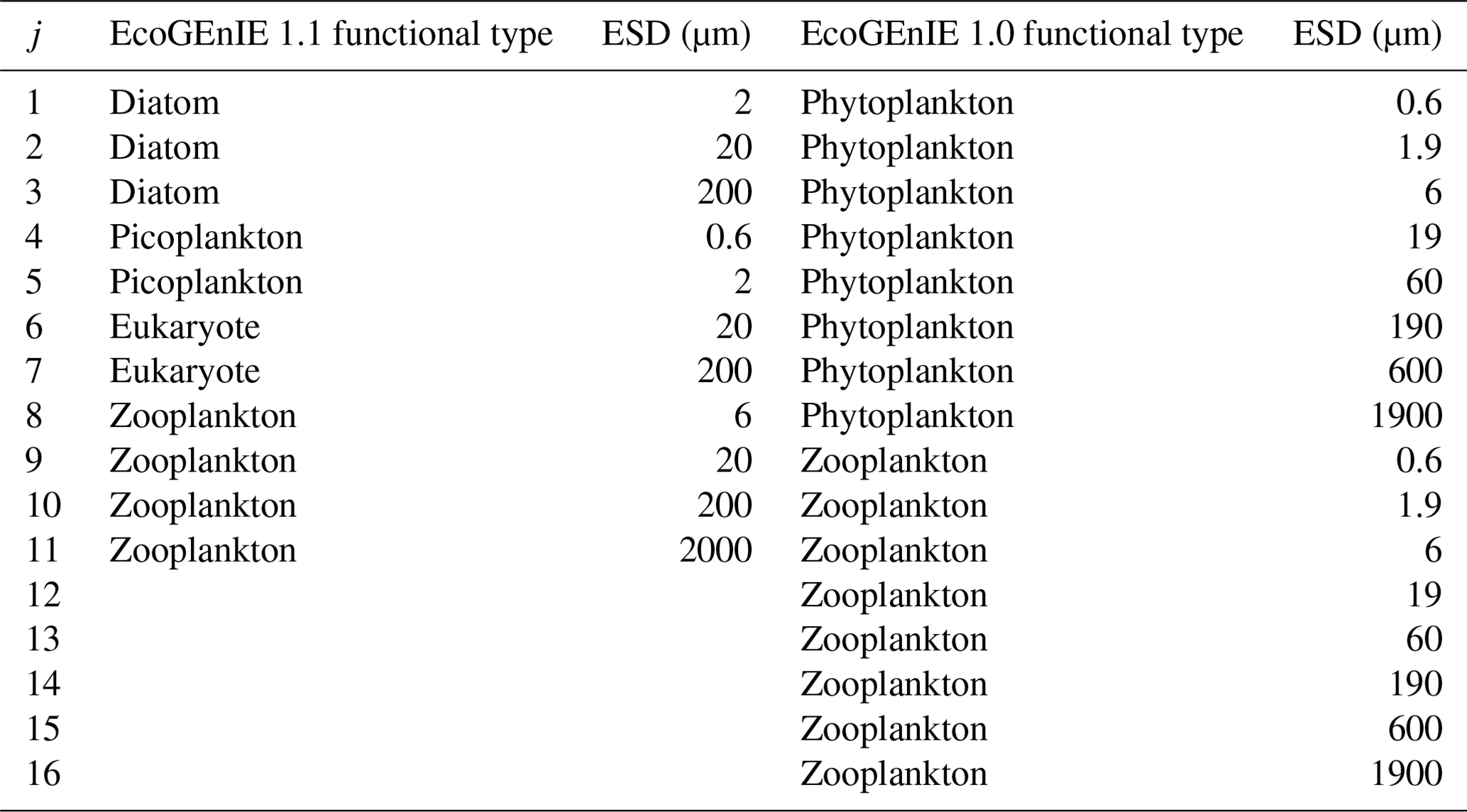
We configure the assumed size structure of the members of the ecosystem differently to Ward et al. (2018) (see Table 1). Specifically, we choose to decrease the number of size classes (four zooplankton instead of eight) and rationalise the remaining structure by, for example, removing the largest phytoplankton and smallest zooplankton size classes, which did not meaningfully persist in the simulations of Ward et al. (2018).
We also tested the impact of the EcoGEnIE 1.0 functional groups and size structure with our new physics and ecosystem tuning in “EcoGEnIE 1.1_phys_eco” (see Sect. 5.1). This allows comparisons of size-diversity range (0.6–1900 µm in EcoGEnIE 1.0 vs. 0.6–2000 µm in EcoGEnIE 1.1) and functional diversity (two functional groups in EcoGEnIE 1.0 vs. four functional groups in EcoGEnIE 1.1). It additionally shows the effect of moving from an allometric unimodal scheme to individual photosynthetic rates with the same physics configuration.
2.4 Diatom physiology
The new parameterisations associated with the incorporation of diatoms in ECOGEM are described below. State variables (nutrient resources, plankton biomass, and organic matter) in EcoGEnIE 1.1 follow the same equations in EcoGEnIE 1.0 and are described in the Supplement.
2.4.1 Size-dependent traits
Power-law functions of organismal volume (Vol =π[Equivalent spherical diameter]3/6) define a given size-dependent parameter (p):
where Vol0 is a reference value of 1 µm3 and a and b are size scaling coefficients. In contrast with EcoGEnIE 1.0, which applies a unimodal photosynthetic uptake rate relationship for all phytoplankton, each phytoplankton functional group within the EcoGEnIE 1.1 population possesses specific rates as per Dutkiewicz et al. (2020), as shown in Table 2.
2.4.2 Diatom extension
As per the other plankton functional groups in the model, diatom biomass (BDiat) varies over time as a balance between a growth term that depends on the uptake rate (V) and limitations by light, temperature, and nutrients as well as loss terms (grazing and mortality), which are fully described in the Supplement.
We used commonly defined diatoms traits and trait trade-offs to characterise their competitiveness relative to other phytoplankton (Tréguer et al., 2021). Defined diatom traits include a higher maximum photosynthetic growth rate () than other phytoplankton (see growth curve in Dutkiewicz et al., 2020), dSi limitation through associated nutrient parameters, and reduced palatability, which is defined by a unitless parameter that modifies the relative grazing palatability on the group (Table 2 and Table S1 and Fig. S6 in the Supplement). Within the model, diatom palatability (0.93) is smaller than for other prey (1), indicative of greater grazing protection. This reduced relative palatability accounts for diatoms' competitive ability to mitigate grazing losses via their protective frustules (Zhang et al., 2017). The model also represents the production of organic matter and biogenic silica (opal) by diatoms, which is exported out of the surface layer after diatom mortality or detritus from feeding.
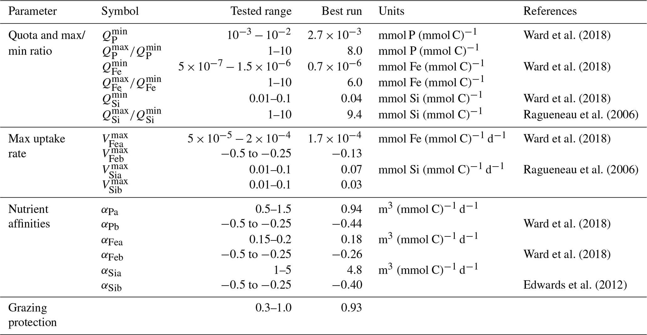
We tuned both the new diatom-specific model parameters and a selection of other ECOGEM parameters related to how general phytoplankton behaviour is controlled (e.g. as related to nutrient acquisition ability). These are listed in Table 2. We compared model results with global ecological and diatom observations (see Sect. 3.2).
3.1 Tuning method
The parameters, whose values we explored in the tuning process, include minimum and maximum nutrient quotas, maximum uptakes rates, and nutrient affinities. We tested a range of values derived from the literature, as summarised in Table 2. We also tuned diatom palatability to best simulate diatom's grazing protection. We kept Ward et al. (2018)'s parameter values for phosphate maximum uptake rate and the cellular carbon quotas, as preliminary sensitivity experiments showed little sensitivity to biogeochemical output (mean oxygen concentration, export production, etc.) when exploring values around the previously well-constrained estimated values (e.g. studies seen in Table 2). We then used Latin hypercube sampling (Mckay et al., 2000) to generate a 550-member ensemble sampling uniformly across the 18 model parameters that we had identified as critical to controlling ecosystem dynamics (and hence marine biogeochemical cycles). For each ensemble member experiment, we calculated an M score (Watterson, 2015) to gauge the model–data fit, with greater values representing better performance:
Here, the model (m) and observational (o) value in the ith ocean grid points (cell) out of a total n grid points are represented by Mi and Oi respectively, with mean-square error described in the numerator. Mean and variance are denoted σ2 and µ respectively. Therefore, the M score is non-dimensional and is a value between zero and one, with higher values indicating better model–data performance.
Table 2List of ECOGEM parameters and Qmax:Qmin (where represents a fixed quota, as the values are equal) selected for tuning and the range of tested values and cited literature.
3.2 Observations
We assessed how successful EcoGEnIE 1.1 was with respect to generating realistic oceanic biogeochemistry by comparing model outputs to observations from the World Ocean Atlas 2013 (WOA13) climatological datasets of dissolved oxygen, phosphate, and dSi (Garcia et al., 2013). This assessment allows direct comparison to the performance assessed in the original description paper of EcoGEnIE (Ward et al., 2018). (Using more up-to-date World Ocean Atlas datasets showed little difference regarding the statistical model performance.) Climatological data were in the form of 1° resolution annual averages that were re-gridded onto the cGEnIE model grid prior to statistical comparison. We also visually contrasted modelled chlorophyll concentrations (whilst also ensuring that they were within the observed range) with an average from 1997 to 2002, measured by the SeaWiFs (Sea-viewing Wide Field-of-view Sensor) satellite (taken from the National Aeronautics and Space Administration Goddard Space Flight Center).
3.3 Model experiments
We created an initial 20 000-year spin-up of the complete system (iron and silica cycles) with the default values from EcoGEnIE 1.0 for the non-silica and diatom-related parameters. Each of the 550 ensemble members was then run for 2000 years, continued from the same ocean biogeochemical and climate steady state. Tests of longer integration times for ensemble member experiments showed that little (<1 %) further change occurred in any M scores for dissolved oxygen, phosphate, or silica beyond 2000 years.
4.1 Model ensemble and justification of parameter set choices
We first considered the statistical performance of all 550 model members vs. observations. Figure 1 shows the results from the tuning ensemble, ordered by the averaged M score across each of the comparisons of the global distributions of dissolved oxygen, phosphate, and silica. Figures 2 and 3 have the same format but now focus in on just the best 50 mean M-score ensemble members with respect to performance. There are clear apparent trade-offs within the mean M-score statistic with, for example, high O2 M scores generally coinciding with lower PO M scores and vice versa (also see Fig. S3). Such a situation could arise, for example, for a “perfect” phosphate cycle but an incorrect carbon-to-phosphate (C : P) ratio, creating a trade-off between PO4 concentrations at intermediate depths tending higher than observations vs. dissolved O2 tending lower than observations. Improving one M score then comes at the expense of the M score of the other. (In such a situation, the silica cycle would be somewhat decoupled from both P and O and, hence, not necessarily exhibit a clear trade-off with either.) We also observe a similar trade-off between the mean ocean oxygen concentration and export production. Thus, while one might select the overall (mean) best M-score experiment when identifying a tuned parameter set with which to go forward, the ability of the model to simulate specific features of the global carbon cycle may also need to be taken into account and will likely depend on the specific application(s) of the tuned model.
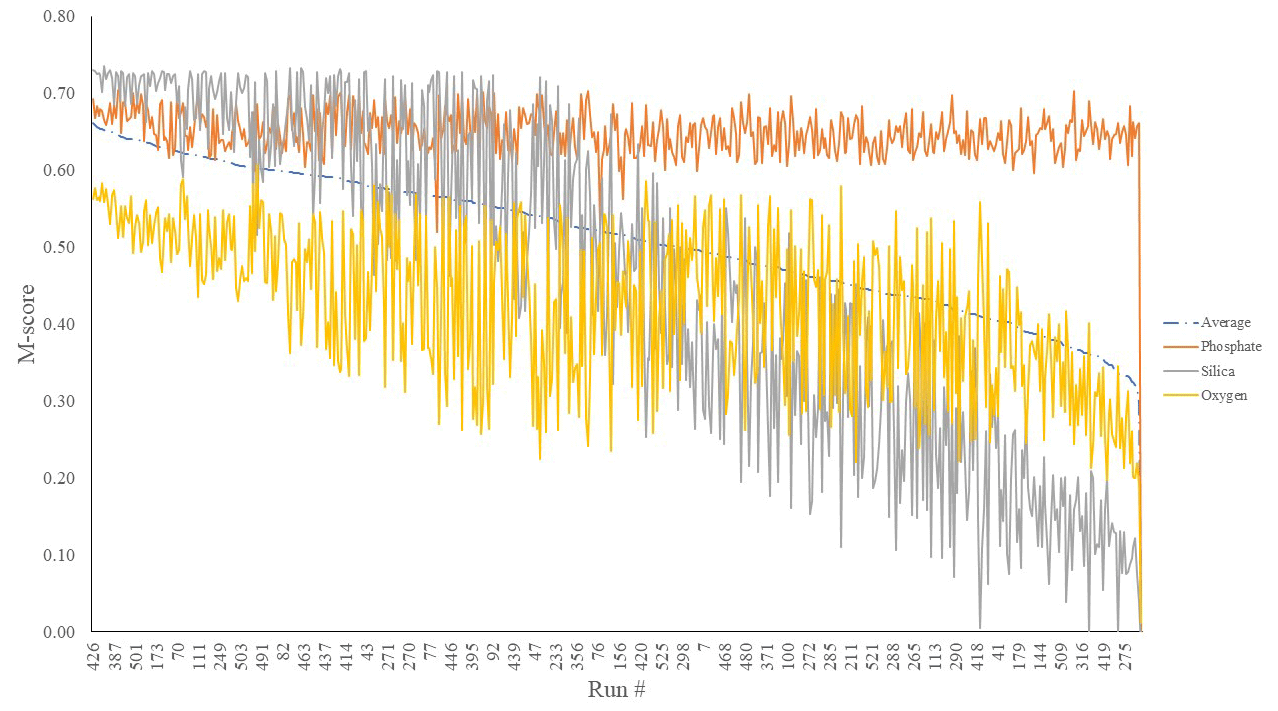
Figure 1M scores of O2 (yellow), SiO2 (grey), and PO4 (orange) mean global ocean concentrations of a 550-run ensemble. The selected run was no. 387 (highest average M score). These scores are calculated by comparing model performance to re-gridded World Ocean Atlas annual average climatologies (Garcia et al., 2013).
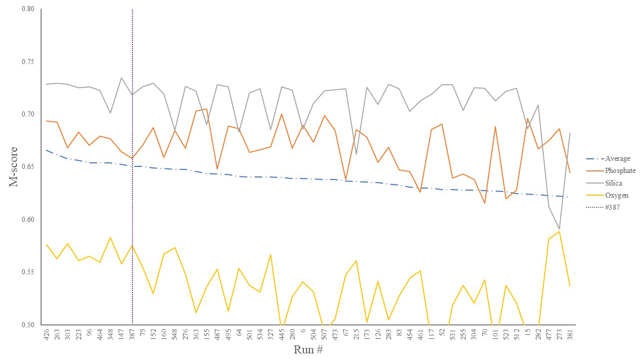
Figure 2Top 50 mean M-score values (dot-dashed line) as well as individual M scores for O2 (yellow), SiO2 (grey), and PO4 (orange) out of the 550-run ensemble. The selected run was no. 387 (highest mean M score).
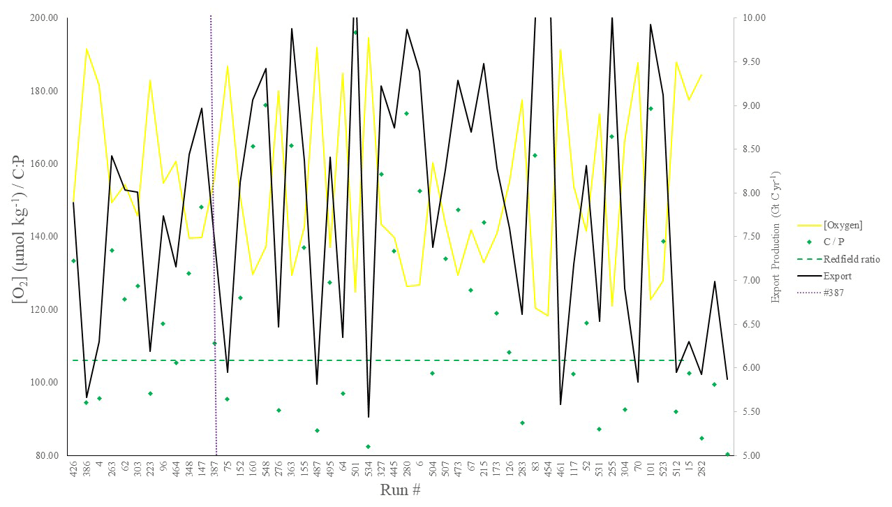
Figure 3POC export (Gt C yr−1), C : P export ratios, and global mean oxygen concentration (µmol kg−1) corresponding to the top 50 runs shown in Fig. 2. Note that both [O2] (yellow line) and C : P (green points) are plotted on the same (left-hand y axis) scale.
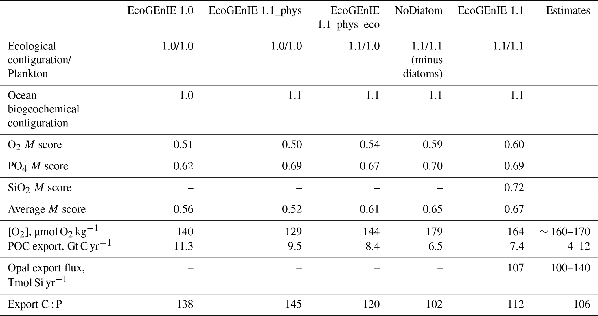
We chose our best run (run no. 387) primarily because it had the highest average M score, although it also considered trade-offs and selected realistic oxygen concentrations (promoted by reasonably low export). We also picked the run with a C : P export ratio close to the Redfield ratio of 106 and recent inverse model estimations of ∼105–113 (Wang et al., 2019; Matsumoto et al., 2020; Teng et al., 2014). This characteristic favoured run no. 387 (global C : P of 112) over the best-performing run with respect to silica (run no. 96), which had a C : P value of 116. While this study primarily concerns diatoms and the silicon cycle, we are also tuning the ecosystem as a whole, necessitating a realistic global C : P value for export. Whilst run no. 464 has a similarly good C : P value and a high average M score, our pick has an opal export value (107 Tmol Si yr−1) within estimates (Table 3) of 100–140 Tmol Si yr−1 (Nelson et al., 1995).
Run no. 387 also produces a global total particulate organic carbon (POC) export of 7.4 Gt C yr−1 (Fig. 3, Table 3), falling well within estimates of 4–12 Gt C yr−1 (Devries and Weber, 2017; Henson et al., 2011; Dunne et al., 2005). The global mean oxygen concentration produced by this iteration is also acceptable at 164 µmol kg−1, close to the ∼170 µmol kg−1 mean calculated from the re-gridded WOA dataset, whilst other statistically high-scoring runs produced values beyond this range (e.g. run no. 426). Such attributes give run no. 387 an average M score of 0.67, making it the best-performing run (Figs. 2, 3).
4.2 Biogeochemical variables
Overall, EcoGEnIE 1.1 captures the zonal contrast in phosphate concentrations between the polar and subpolar regions (>2 µmol P kg−1 towards the poles with ∼1 µmol P kg−1 moving towards the Equator; Fig. 4). The model underestimates phosphate (WOA13 records ∼1 µmol P kg−1) in equatorial and marginal upwelling environments. This partly results from the more simplified physics and lower spatial resolution compared with, for example, current Coupled Model Intercomparison Project (CMIP) models (Séférian et al., 2020). However, the model–data comparison is also not a strictly like-for-like comparison; this is due to the fact that, in re-gridding higher-vertical-resolution WOA data to the model grid, elevated subsurface concentrations become averaged into the re-gridded “surface” layer that cGEnIE is compared against. This will be particularly important in regions where the surface mixed layer is much shallower than 80.8 m. For example, regions with a shallow mixed layer but an elevated subsurface phosphate concentration, such as the equatorial Pacific, appear much more elevated with respect to phosphate in both the re-gridded data and what the model is capable of in terms of nutrient limitation or depletion. Despite this, the model estimates of dSi concentrations in the equatorial upwelling region are reasonable (∼20 µmol Si kg−1), although they fall lower than the re-gridded concentrations present in the surface northern Pacific (∼40 vs. >50 µmol Si kg−1; Fig. 5).
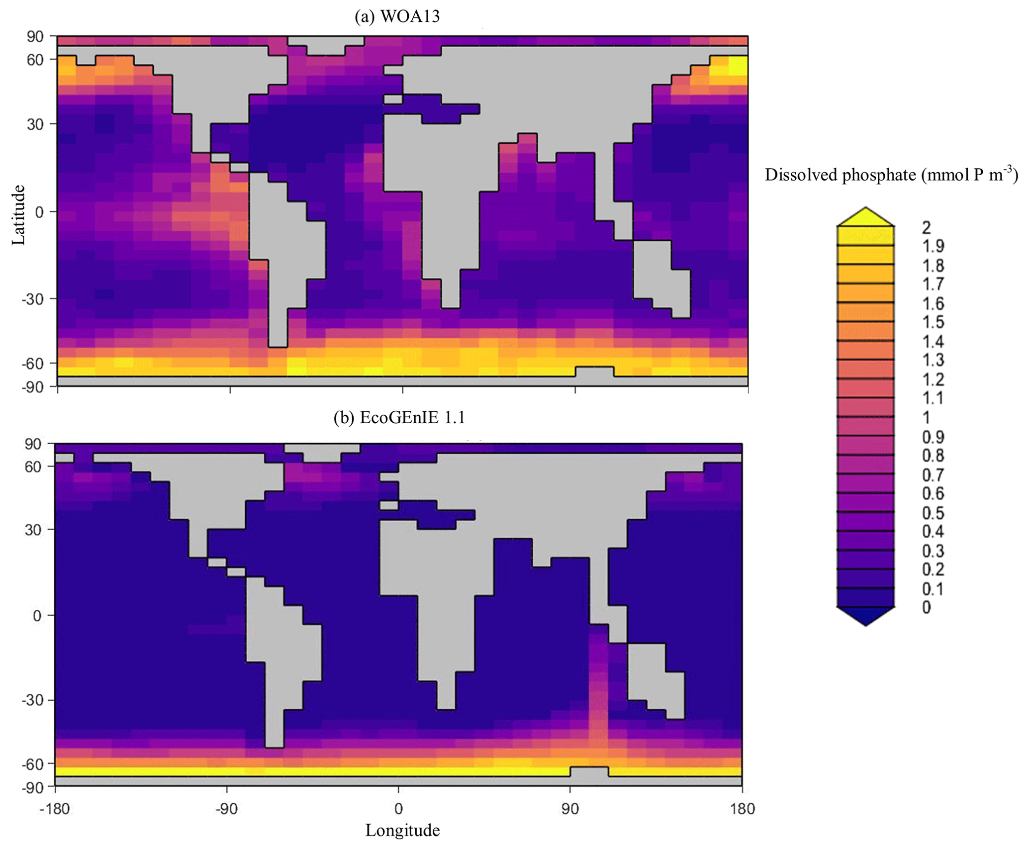
Figure 4Surface concentrations of dissolved phosphate for (a) observations and (b) EcoGEnIE 1.1 output (µmol P kg−1).
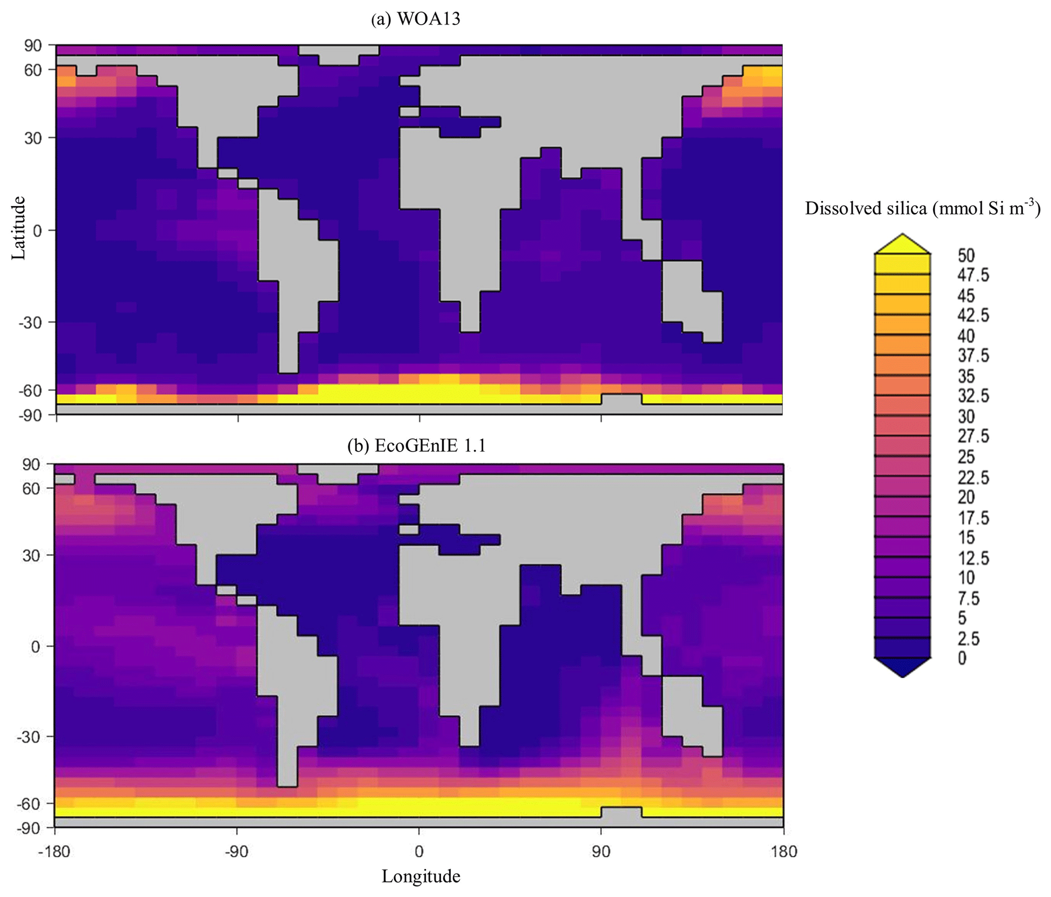
Figure 5Surface concentrations of dSi for (a) observations and (b) EcoGEnIE 1.1 output (µmol Si kg−1).
Through the ocean, EcoGEnIE 1.1 reasonably captures the main features of the vertical biogeochemical tracer distributions in each of the three main ocean basins (Atlantic, Indian, and Pacific). Consistent with observations, the model captures the propagation of dissolved oxygen (∼300 µmol O2 kg−1) at depth through the North Atlantic and Southern Ocean via deep-water formation and transport (Fig. 6). The model performs similarly for phosphate concentrations (Fig. 7) but with a slight underestimation in the intermediate northern Atlantic (which tends towards 0.5 µmol P kg−1 rather than observed values closer to 1 µmol P kg−1 at 1000–3000 m depth). The highest concentrations of phosphate (3 µmol P kg−1) in the equatorial Indian Ocean are seen between 2000 and 4000 m in the observed climatology, where they are limited to <2 km depths in the model, likely due to restricted resolutions at depth and the smaller size of the Indian Basin. The same trends (discrepancies compared with WOA13 are most notable at the greatest depths) are observed in the model for dSi (Fig. 8). However, dSi is generally represented accurately across the three model ocean basins, approaching 0 µmol Si kg−1 in the surface and peaking at approximately 120 µmol Si kg−1 at depths (below 1000 m in the Pacific and Indian oceans).
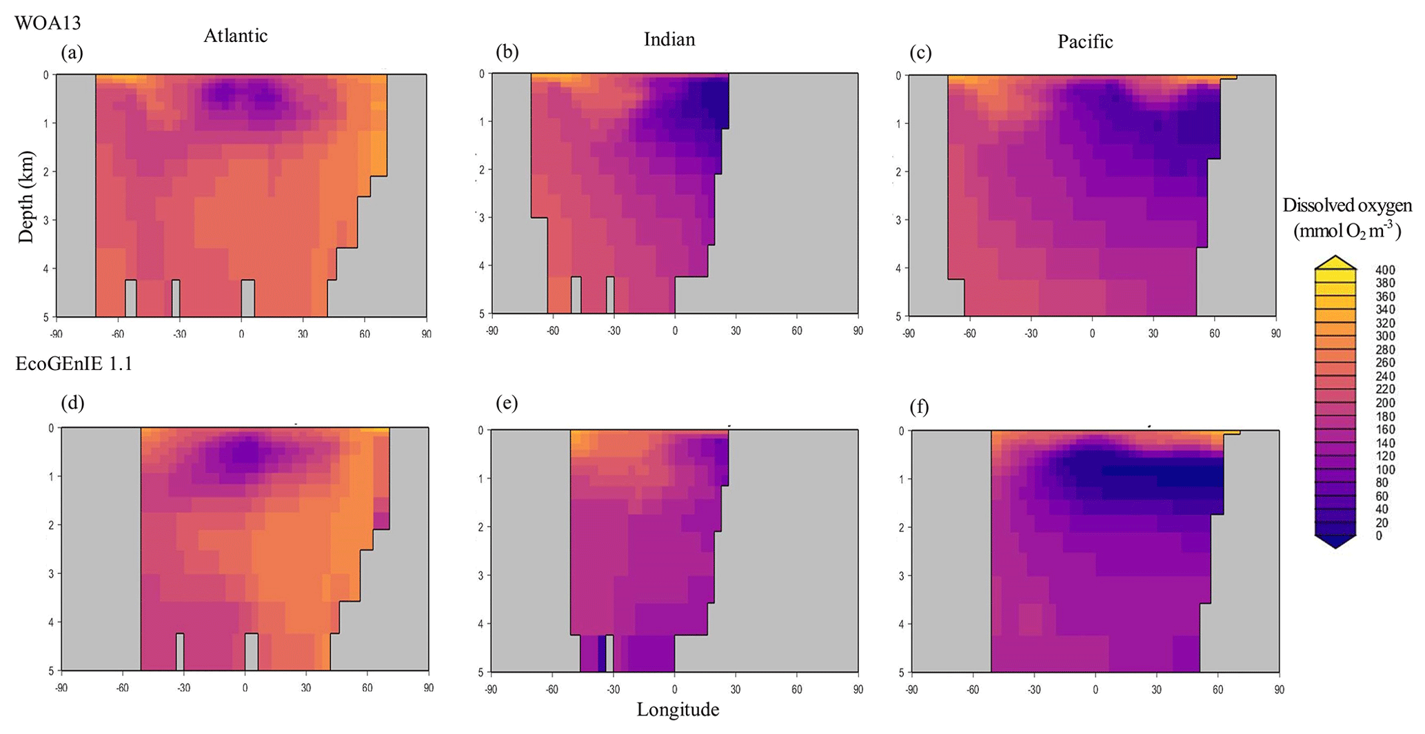
Figure 6Zonally averaged vertical distribution of dissolved oxygen for (d–f) the best EcoGEnIE 1.1 run (µmol O2 kg−1) compared to (a–c) WOA13.
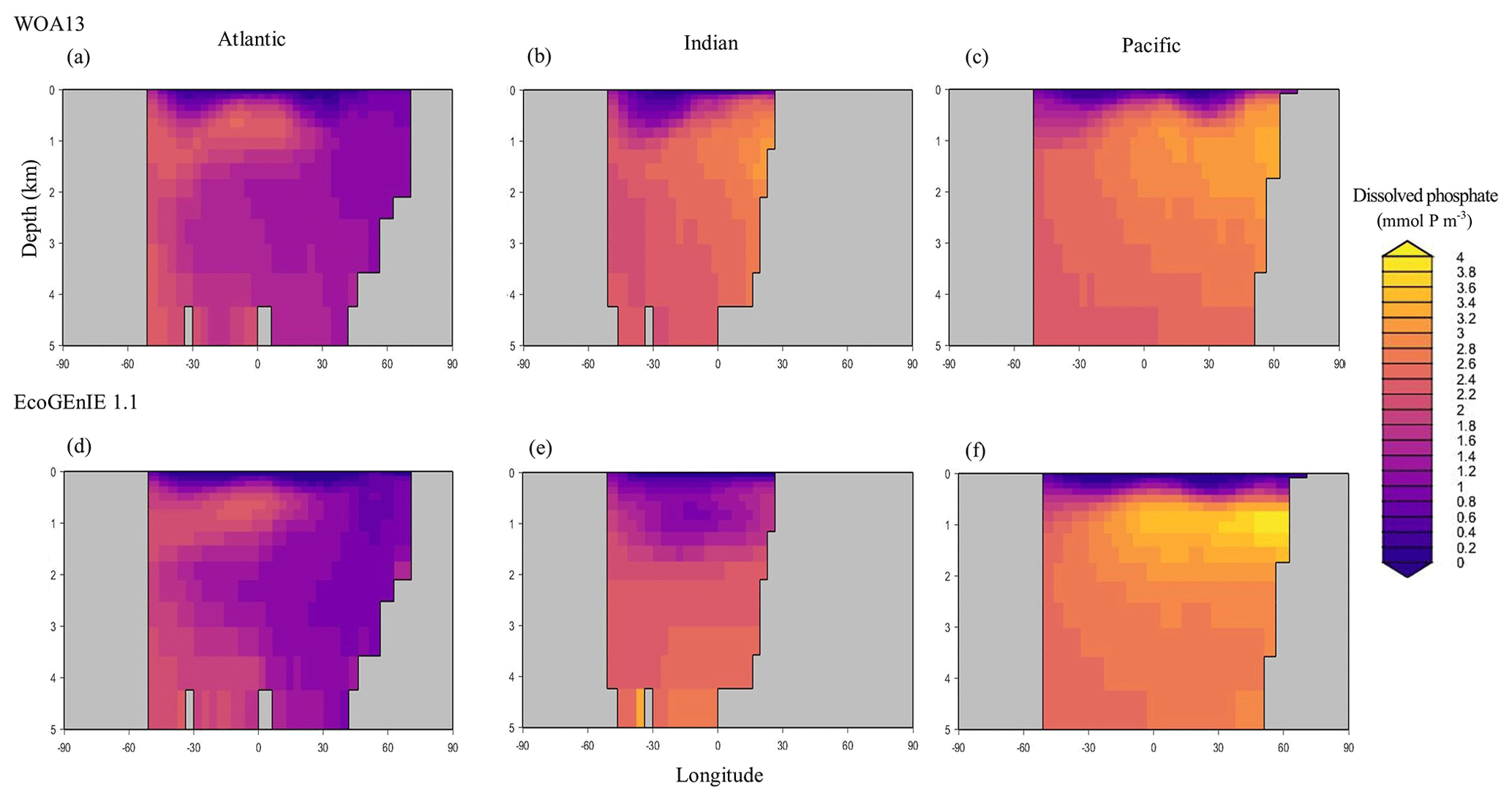
Figure 7Zonally averaged vertical distribution of dissolved phosphate (µmol P kg−1) from (d–f) EcoGEnIE 1.1 compared to (a–c) WOA13.
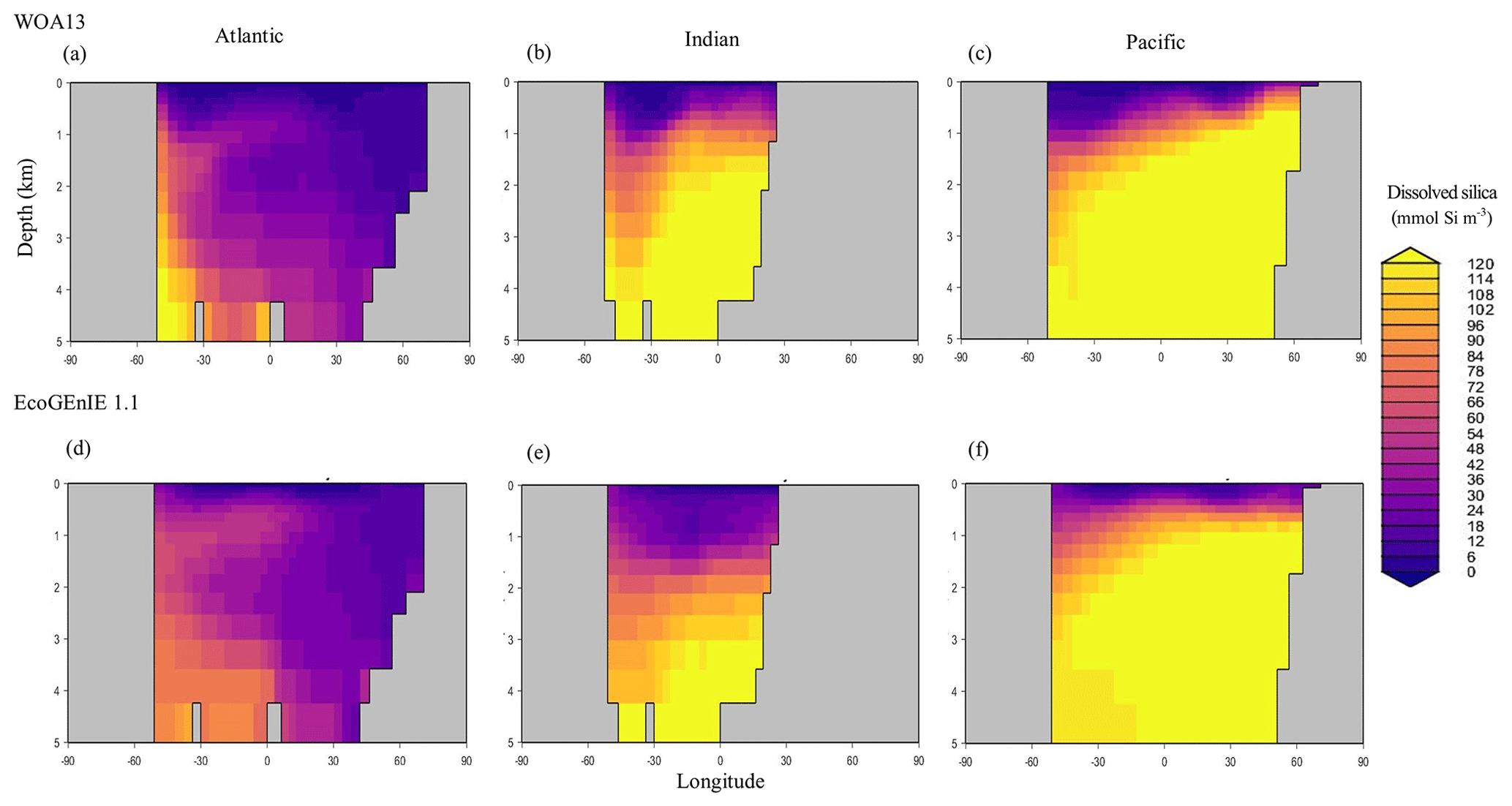
Figure 8Zonally averaged vertical distribution of dSi (µmol Si kg−1) from (d–f) EcoGEnIE 1.1 compared to (a–c) WOA13.
4.3 Ecological variables
We also assessed the performance of the tuned model relative to chlorophyll observations from the SeaWiFs satellite as well as to export production-relevant metrics such as the organic matter C : P (Redfield) ratio. We additionally assessed carbon biomass distributions in our configured plankton community.
Firstly, EcoGEnIE 1.1 chlorophyll (Chl) biomass compares generally well to satellite estimates, peaking at ∼1 mg Chl m−3 in the high latitudes and equatorially. However, there is noticeably low chlorophyll in the eastern boundary upwelling regions in our simulations, which is an issue also visible in EcoGEnIE 1.0. Overall, Figs. 9 and 12d show similar distributions of chlorophyll biomass and total diatom biogeography, with EcoGEnIE 1.1 presenting improved and distinct subtropical gyres from the original rendition. EcoGEnIE 1.1 tends to have more widespread peak Chl values than in the satellite images, with lower Chl in the subtropics and prominent Chl in the Southern Ocean (Fig. 9). However, it is known that satellite observations can underestimate concentrations in the high latitudes (Dierssen, 2010). This could help explain some of the model disagreement in the Southern Ocean. For the Arctic, the sign of the model–data mismatch is reversed and is more likely to be primarily due to the limited model resolution in this basin, reflecting restricted circulation in the model and/or poor seasonal sea-ice cover.
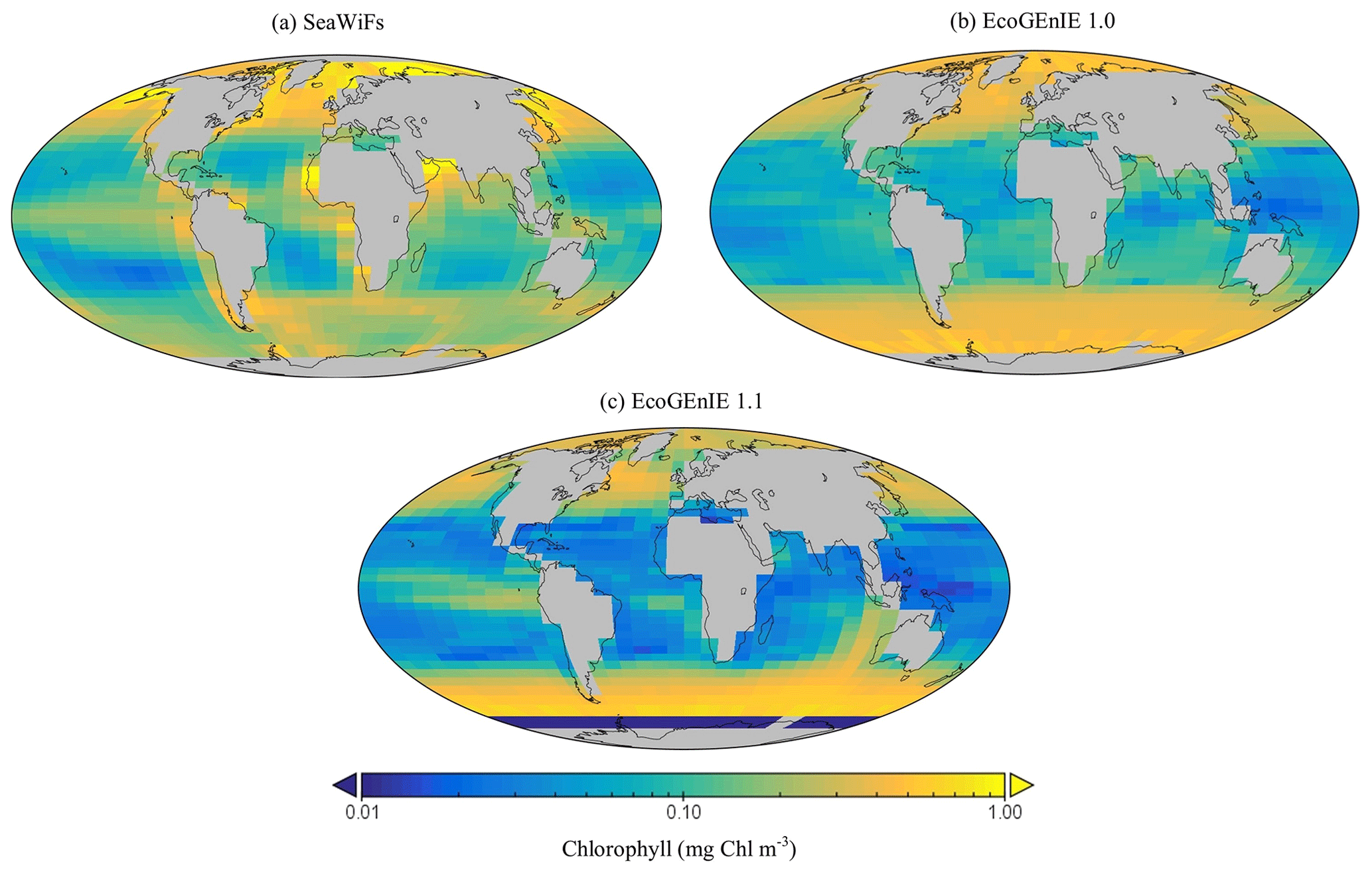
Figure 9The (a) satellite-derived and (b, c) modelled surface chlorophyll-a concentration (mg Chl m−3).
Table 3Performance of the three renditions of EcoGEnIE (EcoGEnIE, NoDiatom, and EcoGEnIE 1.1) and their M scores with respect to WOA13 data. NoDiatom is configured identically to EcoGEnIE 1.1 with just the diatom functional group removed. Two additional runs are shown: one in which our new physics are applied to EcoGEnIE 1.0 (EcoGEnIE 1.1_phys) and another in which our ecosystem tuning and new physics are applied to EcoGEnIE 1.0 (EcoGEnIE 1.1_phys_eco). Both of these aforementioned runs use EcoGEnIE 1.0's plankton population.
Global annual mean POC export in the model is 7.4 Gt C yr−1 (Table 3), which is within the estimated range of 4–12 Gt C yr−1 (Devries and Weber, 2017; Henson et al., 2011; Dunne et al., 2005). Spatially, the modelled POC and opal export reaches relatively high values (>4 mol C m−2 yr−1 and >1 mol Si m−2 yr−1 respectively) in the subpolar regions, such as the Southern Ocean and the northern and eastern equatorial Pacific, and exhibits relatively low values (<1 mol m−2 yr−1) in the subtropical gyres and at high polar latitudes (Fig. 10a). The latter is due to sea-ice formation in the Southern Ocean, which is assumed to prevent light penetration in the model and, hence, limits production, while the low production in the Arctic is likely due to a combination of the seasonal presence of sea-ice cover in the model as well as the very limited model resolution in this region.
The global C : P export ratio is approximately 112 in our preferred model calibration (Table 3), with higher ratios (>120) in the subtropical gyres and low ratios (∼90) in the subpolar and upwelling regions (Fig. 10b). This distribution, at least visually, agrees with previous estimates (Teng et al., 2014; Tanioka et al., 2022) with the exception of the North Atlantic, which has previously been observed to have extremely high values (∼200). One reason that the model struggles to produce these high C : P ratios is because it does not include a nitrogen cycle (and nitrogen fixation); thus, regions where nitrogen concentrations may be low or high (e.g. North Atlantic) may possess unrealistic C : P ratios.
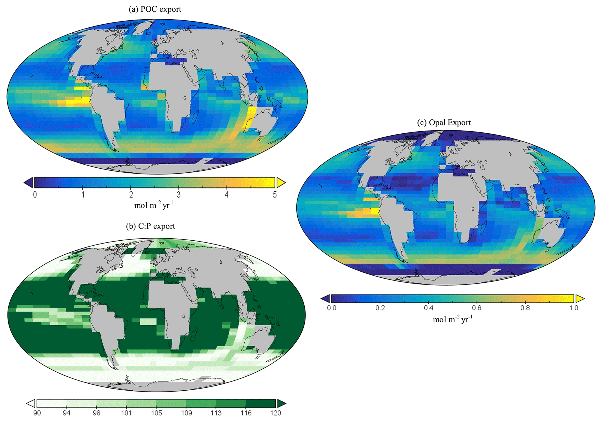
Figure 10Global (a) POC and (c) opal export (mol m−2 yr−1). Global surface distribution of (b) the C : P ratio for the export of particulate organic matter.
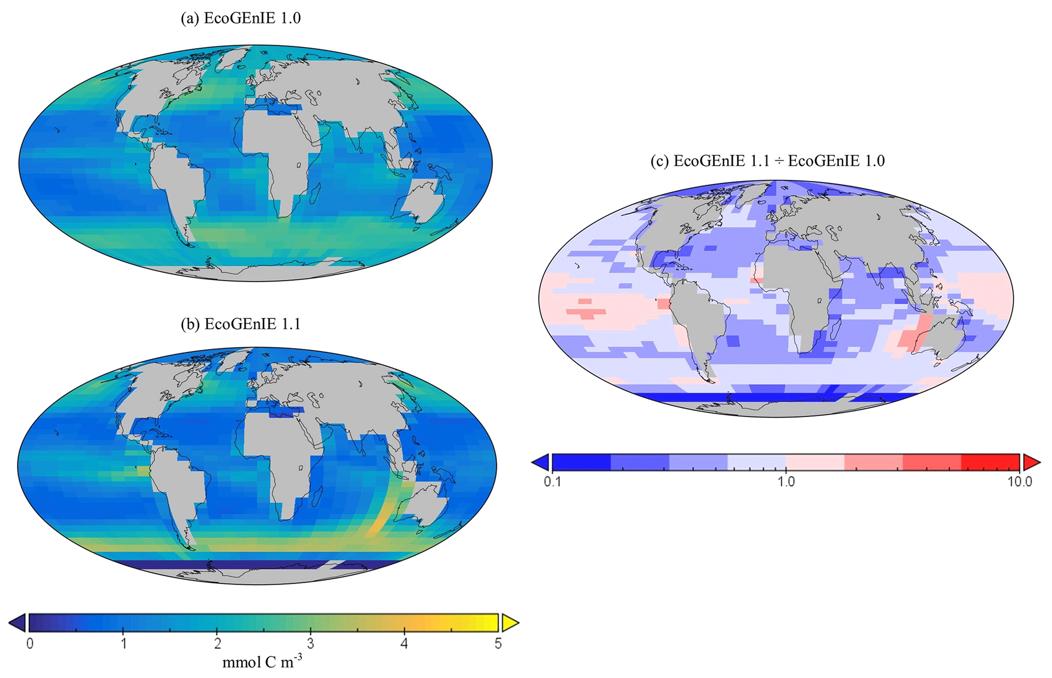
Figure 11Surface concentrations of total carbon biomass for (a) EcoGEnIE 1.0 and (b) EcoGEnIE 1.1 (mmol C m−3). Panel (c) depicts the relative increase or decrease in EcoGEnIE 1.1 from EcoGEnIE 1.0 for vertical fluxes of particulate organic carbon (mmol C m−2 d−1).
The spatial distribution of diatoms (total biomass of all size classes) in EcoGEnIE 1.1 is consistent with previous estimates (Tréguer et al., 2018), with high concentrations in the productive regions (e.g. equatorial upwelling and subpolar regions) and a peak in the Southern Ocean at ∼1 mmol C m−3 (Fig. 12d). However, direct and explicit comparison to ecological datasets as a means of model verification is limited by observational sampling techniques as well as the relatively coarse model ecological size structure (see Sect. 5.2). Diatoms contribute to 18 % of total carbon biomass in the model and 6 % of exported carbon. Of the three different size classes parameterised in the model (Table 1), the smallest (2 µm) is the most cosmopolitan and is abundant across all dSi-enriched regions: the Southern Ocean, equatorial upwelling zones, and the northern subpolar region (Fig. 12a). Their larger counterparts (20 µm) dominate in the subpolar and equatorial upwelling regions (Fig. 12b) and boast a greater peak biomass (0.28 vs. 0.19 mmol C m−3). The 200 µm diatom size class is further restricted with respect to geographical extent, consistent with the fact that, as they increase in size in the model, diatoms become increasingly restricted to dSi-enriched regions, most notably to the Southern Ocean (Fig. 12c). The relative carbon biomass distribution of the 2 and 20 µm diatoms is depicted in Fig. 13. The Southern Ocean presents a dominance of diatoms within the larger size class, with over twice the carbon biomass compared with the 2 µm class. In contrast, equatorial upwelling regions are characterised by a somewhat equal size distribution between the 2 and 20 µm classes, with the 2 µm class having a slightly greater presence. All diatom size classes are virtually absent within the subtropical gyres and low-nutrient regions.
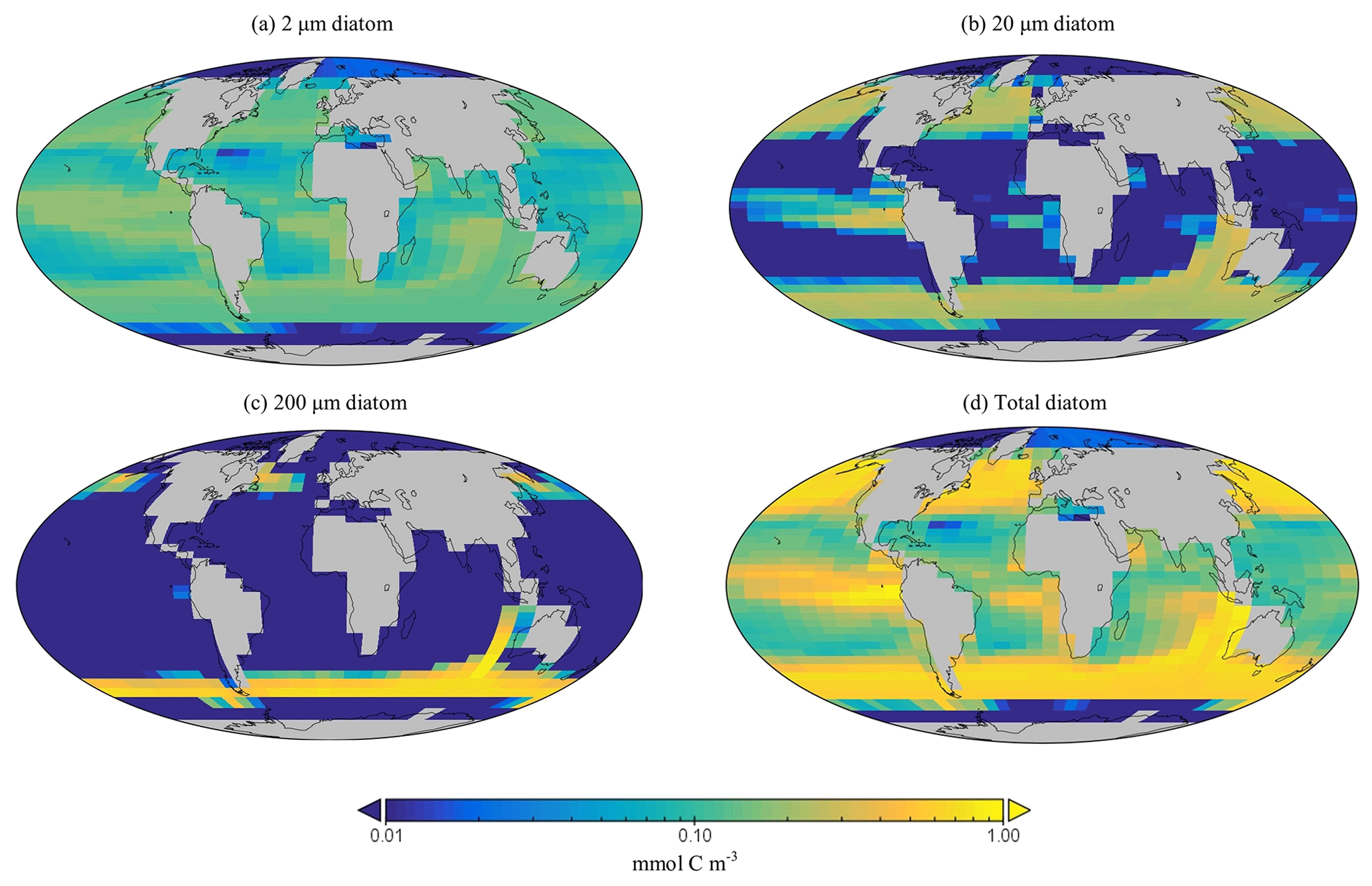
Figure 12Surface concentrations of carbon biomass for (a–c) each diatom size class (mmol C m−3) and (d) their summed biomass.
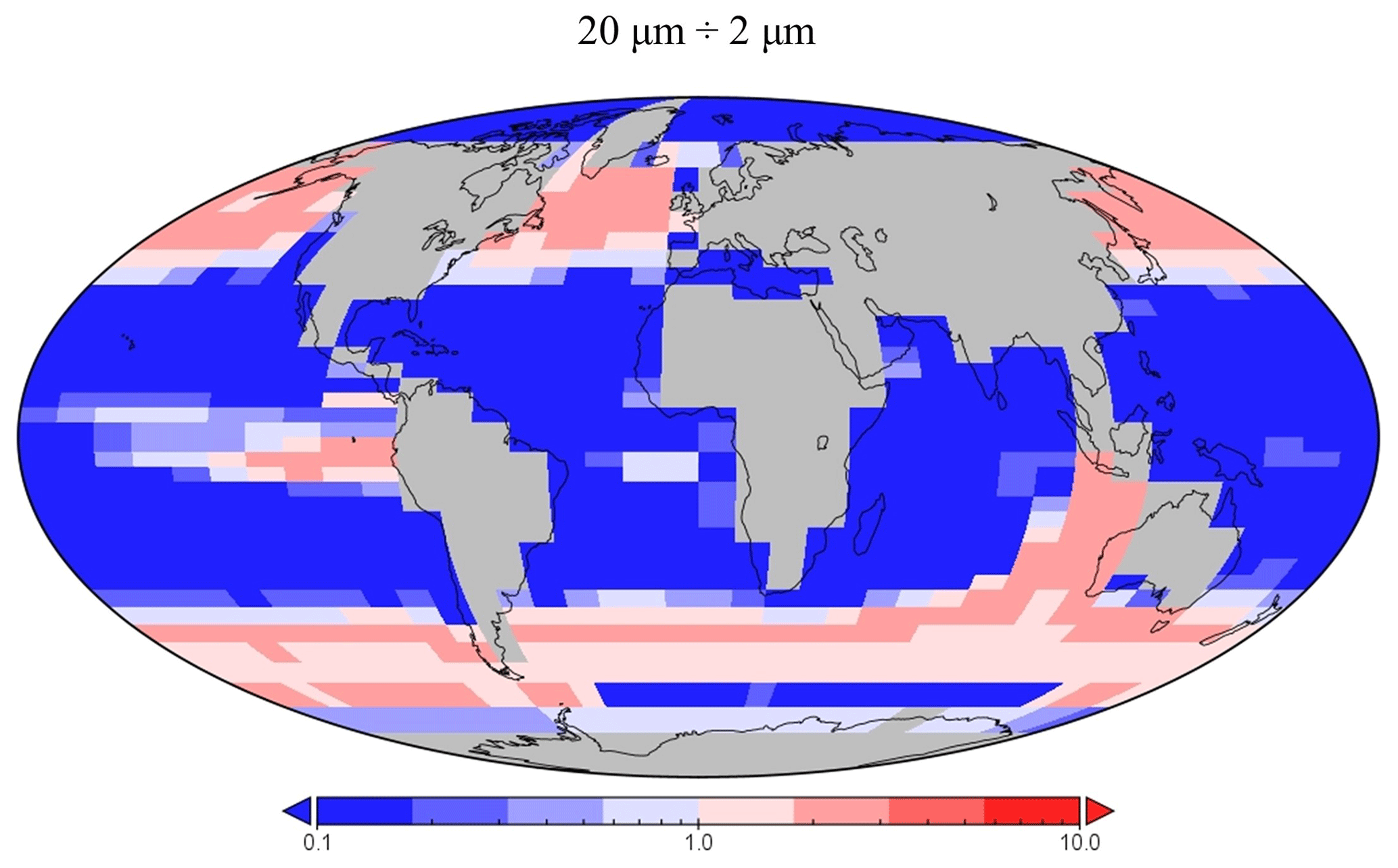
Figure 13The relative presence of diatoms in the 20 µm size class compared with the 2 µm class.
In this section, we assess and discuss how the projections of EcoGEnIE 1.1 compare to EcoGEnIE 1.0, what has changed and why, and pay particular attention to the impact of changing the configuration of the underlying ocean circulation component as well as adding a diatom functional type. We then discuss the capability of EcoGEnIE 1.1 with respect to simulating diatom biogeography within size classes.
5.1 EcoGEnIE 1.0 vs. EcoGEnIE 1.1
We first directly contrast EcoGEnIE 1.1 model outputs with the previous and original ecological version – EcoGEnIE 1.0 (Ward et al., 2018), with the latter including eight size classes of phytoplankton and zooplankton as well as employing different ocean physics. We then assess the impact of the individual changes that we have made (new physics, ecosystem tuning, and size structure change with new functional groups) in runs defined within this section and Table 3 (NoDiatom, EcoGEnIE 1.1_phys, and EcoGEnIE 1.1_phys_eco).
Relative to EcoGEnIE 1.0, EcoGEnIE 1.1 performs better for all of the biogeochemical tracers. The EcoGEnIE 1.1 mean oxygen concentration is more realistic than in EcoGEnIE 1.0 (164 vs. 140 µmol O2 kg−1), which is a direct consequence of lower export production rates (7.4 vs. 11.3 Gt C yr−1) and, hence, reduced respiration in the water column. Basin profiles in EcoGEnIE 1.0 (Fig. 14) also exhibited somewhat unrealistic elevated and widespread dysoxia in the low-latitude and northern regions of the Indian Ocean. Again, in EcoGEnIE 1.0, this was likely due to the enhanced export (leading to greater oxygen consumption at intermediate depths).
Despite a lower total global export flux in EcoGEnIE 1.1, specific regions – notably equatorial upwelling areas – have higher export relative to EcoGEnIE 1.0 (Fig. 15a). Similar patterns are also seen in the NoDiatom run (which is identically configured to EcoGEnIE 1.1 – same functional groups, size structure, and physics – but with no diatom functional group) export distribution which has lower production in the equatorial region than EcoGEnIE 1.1 (Fig. 15b), suggesting that the difference is primarily due to the change in ocean physics (Fig. S5). In other regions, the change in ecological configuration appears to dominate and the absence of diatoms in NoDiatom intuitively results in a Southern Ocean with lower export production than in EcoGEnIE 1.1 under the same physics conditions.
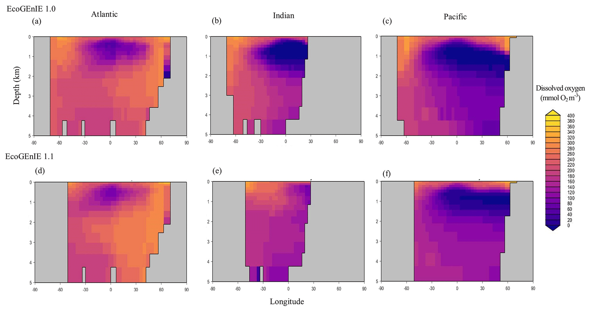
Figure 14Zonally averaged vertical distribution of dissolved oxygen for (d–f) the best EcoGEnIE 1.1 run (µmol O2 kg−1) compared with (a–c) EcoGEnIE 1.0.
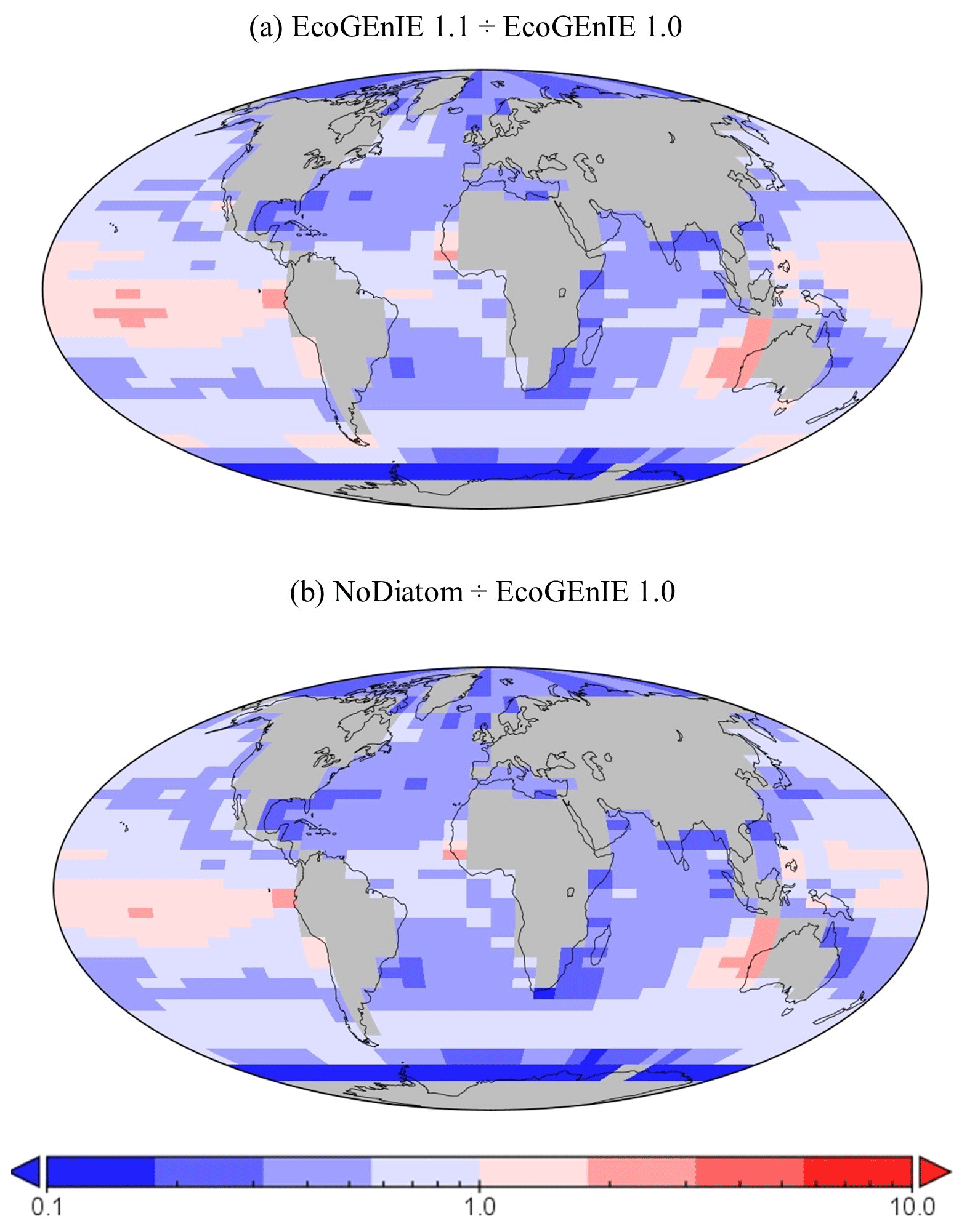
Figure 15The relative increase or decrease in (a) EcoGEnIE 1.1 from EcoGEnIE and (b) NoDiatom from EcoGEnIE 1.0 for vertical fluxes of particulate organic carbon (mmol C m−2 d−1).
Another improvement apparent in EcoGEnIE 1.1 and NoDiatom compared with EcoGEnIE 1.0 is the C : P export ratio (Table 3), which is pushed significantly closer to the Redfield value of 106, likely thanks to the tuning of Qmin and Qmax values performed in this study to produce more realistic stoichiometries. Such results imply that the steps taken in to refine the model have produced more realistic and comprehensive biogeochemical interactions within the water column. We suspect that the re-tuning of C : P export ratio to ∼112 helped EcoGEnIE 1.1 to produce more favourable basin profiles.
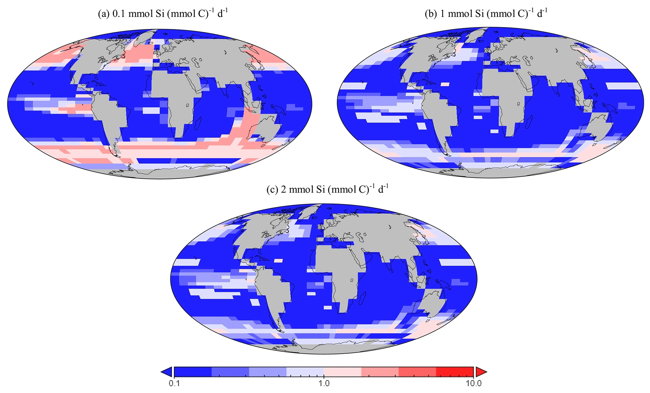
Figure 16Sensitivity testing for dSi uptake rates of diatoms within EcoGEnIE 1.1. Panels (a) to (c) depict the relative presence of diatoms in the 20 µm size class compared with the 2 µm class. Thus, values above one indicate a region dominated by larger diatoms.
Going from EcoGEnIE 1.0 to EcoGEnIE 1.1, there is a clear improvement in the distinction between low biomass in subtropical gyres and high biomass at higher latitudes (Fig. 11), which can be attributed principally to the modified ocean physics (both NoDiatom and EcoGEnIE 1.1 share close similarities and are distinct from EcoGEnIE 1.0). The EcoGEnIE 1.1 southernmost region of the Southern Ocean has lower POC export than the previous version (Fig. 11c). This result probably comes from the new sea-ice module in which growth is no longer enabled at these high latitudes. The POC export reduction above the Southern Ocean is due to the new physics, where subtropical gyres are better defined and, subsequently, plankton growth is more restricted in these now nutrient-replete regions. The equatorial chlorophyll biomass of EcoGEnIE 1.1 shows a noticeable increase from the original rendition (Fig. 9), producing results closer to satellite estimates (Fig. S4). The introduction of diatoms moving from NoDiatom and EcoGEnIE 1.1 is also notably felt in the Southern Ocean, likely due to the high concentrations of dSi which can only be utilised by diatoms in EcoGEnIE 1.1, as they are not present in NoDiatom. Overall (with the exception of the Southern Ocean and equatorial upwelling areas), there are only relatively marginal changes between the EcoGEnIE 1.1 and NoDiatom runs (relative to the change from EcoGEnIE 1.0 to 1.1), suggesting that, in the absence of diatoms, other phytoplankton can take advantage of these vacant niches that diatoms would otherwise compete in. With our trait-based approach enabling size diversity amongst functional types, it is intuitive that plankton of the same sizes as the diatom classes would make up the difference with regards to the primary production deficit (i.e. size is the master trait), although they cannot reach similar productive output to diatoms in dSi-rich regions (e.g. the Southern Ocean).
The differences between EcoGEnIE 1.0 and EcoGEnIE 1.1 arise both due to the developments with respect to adding phytoplankton functional groups, changing size structure, and tuning the ECOGEM and switching the physics.
Table 3 includes a run in which the Ward et al. (2018) ecosystem (EcoGEnIE 1.0's functional groups, size structure, and ecosystem tuning) was combined with our new physics; this run is called EcoGEnIE 1.1_phys. On the other hand, EcoGEnIE 1.1_phys_eco also has our new physics and still uses EcoGEnIE 1.0's functional groups and size structure but incorporates our ecosystem tuning. With the exact same ecological structure and parameter tuning as EcoGEnIE 1.0, we found that EcoGEnIE 1.1_phys only achieved slightly improved model correspondence to observations for phosphate, with the oxygen M score drastically decreasing There is, however, a decrease in export production (11.3 vs. 9.5 Gt C yr−1), suggesting that the change in physics helped to improve this result. EcoGEnIE 1.1_phys_eco also shows slight improvements to the phosphate M score; it is likely that our ecosystem tuning somewhat complements the EcoGEnIE 1.0 plankton community due to the similar size range diversity. Once we introduce our non-diatom functional groups (NoDiatom) coupled with the new physics, it is evident how much the results improve (M scores, export, etc.). Adding the diatom functional group (and, thus, ecologically enabling the silica cycle) then improved the M scores further with reasonable opal export.
5.2 Relative diatom distribution
EcoGEnIE 1.1 produced diatom populations in which the smallest size class (2 µm) are the most dominant, a result that agrees with the relatively few observational estimates that are available, as we will discuss next.
Genomic ribotype reads and one in situ plankton recording in the northern Atlantic observe smaller diatoms to be more abundant than larger ones (Barton et al., 2013; Malviya et al., 2016), a characteristic we also find in EcoGEnIE 1.1, although relative northern Atlantic abundance within the model (2 µm diatoms relative to the 20 µm diatoms) is 2 orders of magnitude greater than these recordings. However, studies such as these tend to be poorly constrained via instrumentation, as meshes cannot sample plankton <20 µm, potentially resulting in a significant part of the plankton community remaining unrecorded. This could explain at least partly why EcoGEnIE 1.1 produces seemingly unrealistic relative abundances. Sensitivity testing in the model suggests that the proportion of these size classes depends on the uptake rate for dSi, (Fig. 16). As increases, the ratio of carbon biomass attributed to 20 µm compared with 2 µm biomass decreases. This is intuitive: the allometric relationships within functional groups result in larger plankton becoming less competitive as their nutrient quotas and uptake rates increase metabolic demand. There is a notable absence of the 200 µm diatom class in the northern Atlantic, despite recordings by Barton et al. (2013), suggesting that EcoGEnIE 1.1 struggles to represent larger plankton.
The difficulties associated with assessing the ecological performance of EcoGEnIE 1.0 persist in EcoGEnIE 1.1; these are mostly linked to the nature of ecological community observations and recordings. For example, with plankton biomass restricted to the upper layer (80.8 m) of the GEnIE ocean circulation model grid, direct comparisons to data collected in situ can be somewhat difficult, with satellite estimates inferring concentrations from the surface itself. In situ measurements of diatom distribution tend to opt for ribotype reads of size classes along expedition transects (Malviya et al., 2016); consequently, we are restricted to inferences of regional patterns amongst classes, as opposed to direct comparisons of global population.
5.3 Conclusion
This paper builds on the EcoGEnIE 1.0 model of Ward et al. (2018), which developed a size-based formulation of plankton ecology and embedded this in an Earth system model of intermediate complexity. We expanded the model to include a diatom functional group and other phytoplankton functional groups and, hence, enable the marine silica cycle to be simulated. We not only tuned the model parameters for diatoms but also re-tuned the most critical physiological parameters in the ecosystem model framework, identifying a parameter configuration that performed best towards observations of biogeochemical tracers and ecological variables.
The EcoGEnIE 1.1 model successfully incorporated diatoms as a functional type, enabling dSi as a limiting resource. The competitive nature and success of diatoms is captured in the model, as they are a prevalent group within our configured community (∼20 % of total biomass). With this new extension, there is a potential for further study regarding the ecological success of diatoms during future and past climatological perturbation and their role in the biological pump. For example, with these additions, this model could be utilised to explore the Cenozoic evolution of diatoms and their ongoing influence over the silicon cycle, long-term silica cycling (e.g. residence times), and their associated proxies (Conley et al., 2017; Tréguer et al., 2021). This study also acts as an example of the adaptability of the EcoGEnIE model, encouraging those looking to incorporate additional functional groups into the framework.
The code for the version of the “muffin” release of the cGEnIE Earth system model used in this paper is provided at https://www.seao2.info/cgenie/docs/muffin.pdf (Ridgwell, 2022). Configuration files for the specific experiments presented in the paper can be found via the following DOI: https://doi.org/10.5281/zenodo.10223295 (newest version) (Ridgwell et al., 2023). Details of the experiments, as well as the command line needed to run each one, are given in the readme.txt file in that directory. All other configuration files and boundary conditions are provided as part of the code release. A manual detailing code installation, basic model configuration, tutorials covering various aspects of model configuration, experimental design, and output as well as the processing of results can be found at https://www.seao2.info/cgenie/docs/muffin.pdf (Ridgwell, 2022).
The supplement related to this article is available online at: https://doi.org/10.5194/gmd-17-1729-2024-supplement.
AANB tuned the model under the supervision of FMM with respect to the ecosystem. The iron biogeochemistry was developed by AR and JDW. KRH and DJC provided their expertise regarding the silicon cycle. BAW provided advice regarding the configuration of EcoGEnIE. All authors contributed to the writing of this paper.
The contact author has declared that none of the authors has any competing interests.
Publisher’s note: Copernicus Publications remains neutral with regard to jurisdictional claims made in the text, published maps, institutional affiliations, or any other geographical representation in this paper. While Copernicus Publications makes every effort to include appropriate place names, the final responsibility lies with the authors.
We thank Rhiannon Jones for early discussions regarding the silicon cycle modelling. This research has received funding from the European Research Council (ERC) within the framework of the Horizon 2020 Research and Innovation programme (grant no. 833454, DEVOCEAN). Katharine R. Hendry thanks European Research Council ERC-ICY-LAB (grant no. 678371). Fanny M. Monteiro is grateful to NERC for its funding (grant nos. NE/N011708/1, NE/V01823X/1, and NE/X001261/1). Jamie D. Wilson acknowledges support from the AXA Research Fund. Andy Ridgwell acknowledges support from the National Science Foundation (grant no. EAR-2121165) and the NASA Interdisciplinary Consortia for Astrobiology Research (ICAR) programme (grant no. 80NSSC21K0594).
This research has been supported by the H2020 European Research Council (grant no. 833454, DEVOCEAN).
This paper was edited by Paul Halloran and reviewed by two anonymous referees.
Albani, S., Mahowald, N. M., Murphy, L. N., Raiswell, R., Moore, J. K., Anderson, R. F., McGee, D., Bradtmiller, L. I., Delmonte, B., Hesse, P. P., and Mayewski, P. A.: Paleodust variability since the Last Glacial Maximum and implications for iron inputs to the ocean, Geophys. Res. Lett., 43, 3944–3954, https://doi.org/10.1002/2016gl067911, 2016.
Assmy, P., Smetacek, V., Montresor, M., Klaas, C., Henjes, J., Strass, V. H., Arrieta, J. M., Bathmann, U., Berg, G. M., Breitbarth, E., Cisewski, B., Friedrichs, L., Fuchs, N., Herndl, G. J., Jansen, S., Krägefsky, S., Latasa, M., Peeken, I., Röttgers, R., Scharek, R., Schüller, S. E., Steigenberger, S., Webb, A., and Wolf-Gladrow, D.: Thick-shelled, grazer-protected diatoms decouple ocean carbon and silicon cycles in the iron-limited Antarctic Circumpolar Current, P. Natl. Acad. Sci. USA, 110, 20633–20638, https://doi.org/10.1073/pnas.1309345110, 2013.
Banse, K.: Cell volumes, maximal growth rates of unicellular algae and ciliates, and the role of ciliates in the marine pelagial1,2, Limnol. Oceanogr., 27, 1059–1071, https://doi.org/10.4319/lo.1982.27.6.1059, 1982.
Cao, L., Eby, M., Ridgwell, A., Caldeira, K., Archer, D., Ishida, A., Joos, F., Matsumoto, K., Mikolajewicz, U., Mouchet, A., Orr, J. C., Plattner, G.-K., Schlitzer, R., Tokos, K., Totterdell, I., Tschumi, T., Yamanaka, Y., and Yool, A.: The role of ocean transport in the uptake of anthropogenic CO2, Biogeosciences, 6, 375–390, https://doi.org/10.5194/bg-6-375-2009, 2009.
Conley, D. J., Frings, P. J., Fontorbe, G., Clymans, W., Stadmark, J., Hendry, K. R., Marron, A. O., and De La Rocha, C. L.: Biosilicification Drives a Decline of Dissolved Si in the Oceans through Geologic Time, Front. Mar. Sci., 4, 397, https://doi.org/10.3389/fmars.2017.00397, 2017.
Crichton, K. A., Wilson, J. D., Ridgwell, A., and Pearson, P. N.: Calibration of temperature-dependent ocean microbial processes in the cGENIE.muffin (v0.9.13) Earth system model, Geosci. Model Dev., 14, 125–149, https://doi.org/10.5194/gmd-14-125-2021, 2021.
Devries, T. and Weber, T.: The export and fate of organic matter in the ocean: New constraints from combining satellite and oceanographic tracer observations, Global Biogeochem. Cy., 31, 535–555, https://doi.org/10.1002/2016gb005551, 2017.
Dierssen, H. M.: Perspectives on empirical approaches for ocean color remote sensing of chlorophyll in a changing climate, P. Natl. Acad. Sci. USA, 107, 17073–17078, https://doi.org/10.1073/pnas.0913800107, 2010.
Dunne, J. P., Armstrong, R. A., Gnanadesikan, A., and Sarmiento, J. L.: Empirical and mechanistic models for the particle export ratio, Global Biogeochem. Cy., 19, https://doi.org/10.1029/2004gb002390, 2005.
Dutkiewicz, S., Cermeno, P., Jahn, O., Follows, M. J., Hickman, A. E., Taniguchi, D. A. A., and Ward, B. A.: Dimensions of marine phytoplankton diversity, Biogeosciences, 17, 609–634, https://doi.org/10.5194/bg-17-609-2020, 2020.
Falkowski, P. G., Katz, M. E., Knoll, A. H., Quigg, A., Raven, J. A., Schofield, O., and Taylor, F. J. R.: The Evolution of Modern Eukaryotic Phytoplankton, Science, 305, 354–360, https://doi.org/10.1126/science.1095964, 2004.
Field, C. B., Behrenfeld, M. J., Randerson, J. T., and Falkowski, P.: Primary Production of the Biosphere: Integrating Terrestrial and Oceanic Components, Science, 281, 237–240, https://doi.org/10.1126/science.281.5374.237, 1998.
Follows, M. J. and Dutkiewicz, S.: Modeling Diverse Communities of Marine Microbes, Annu. Rev. Mar. Sci., 3, 427–451, https://doi.org/10.1146/annurev-marine-120709-142848, 2011.
Follows, M. J., Dutkiewicz, S., Grant, S., and Chisholm, S. W.: Emergent Biogeography of Microbial Communities in a Model Ocean, Science, 315, 1843–1846, https://doi.org/10.1126/science.1138544, 2007.
Friedrichs, M. A. M., Dusenberry, J. A., Anderson, L. A., Armstrong, R. A., Chai, F., Christian, J. R., Doney, S. C., Dunne, J., Fujii, M., Hood, R., McGillicuddy, D. J., Moore, J. K., Schartau, M., Spitz, Y. H., and Wiggert, J. D.: Assessment of skill and portability in regional marine biogeochemical models: Role of multiple planktonic groups, J. Geophys. Res., 112, https://doi.org/10.1029/2006jc003852, 2007.
Garcia, H. E., Locarnini, R. A., Boyer, T. P., Antonov, J. I., Baranova, O. K., Zweng, M. M., Reagan, J. R., Johnson, D. R., Mishonov, A. V., and Levitus, S.: World ocean atlas 2013. Volume 4, Dissolved inorganic nutrients (phosphate, nitrate, silicate), NOAA Atlas NESDIS, 76, https://doi.org/10.7289/V5J67DWD, 2013.
Hendry, K. R., Marron, A. O., Vincent, F., Conley, D. J., Gehlen, M., Ibarbalz, F. M., Quéguiner, B., and Bowler, C.: Competition between Silicifiers and Non-silicifiers in the Past and Present Ocean and Its Evolutionary Impacts, Front. Mar. Sci., 5, 22, https://doi.org/10.3389/fmars.2018.00022, 2018.
Henson, S. A., Sanders, R., Madsen, E., Morris, P. J., Le Moigne, F., and Quartly, G. D.: A reduced estimate of the strength of the ocean's biological carbon pump, Geophys. Res. Lett., 38, https://doi.org/10.1029/2011gl046735, 2011.
Kiørboe, T., Visser, A., and Andersen, K. H.: A trait-based approach to ocean ecology, ICES J. Mar. Sci., 75, 1849–1863, https://doi.org/10.1093/icesjms/fsy090, 2018.
Kraus, E. B. and Turner, J. S.: A one-dimensional model of the seasonal thermocline II. The general theory and its consequences, Tellus, 19, 98–106, https://doi.org/10.3402/tellusa.v19i1.9753, 1967.
Kriest, I., Khatiwala, S., and Oschlies, A.: Towards an assessment of simple global marine biogeochemical models of different complexity, Prog. Oceanogr., 86, 337–360, https://doi.org/10.1016/j.pocean.2010.05.002, 2010.
Kwiatkowski, L., Yool, A., Allen, J. I., Anderson, T. R., Barciela, R., Buitenhuis, E. T., Butenschön, M., Enright, C., Halloran, P. R., Le Quéré, C., de Mora, L., Racault, M.-F., Sinha, B., Totterdell, I. J., and Cox, P. M.: iMarNet: an ocean biogeochemistry model intercomparison project within a common physical ocean modelling framework, Biogeosciences, 11, 7291–7304, https://doi.org/10.5194/bg-11-7291-2014, 2014.
Lavaud, J., Rousseau, B., and Etienne, A.-L.: General features of photoprotection by energy dissipation in planktonic diatoms (bacillariophyceae)1, J. Phycol., 40, 130–137, https://doi.org/10.1046/j.1529-8817.2004.03026.x, 2004.
Mahowald, N., Kohfeld, K., Hansson, M., Balkanski, Y., Harrison, S. P., Prentice, I. C., Schulz, M., and Rodhe, H.: Dust sources and deposition during the last glacial maximum and current climate: A comparison of model results with paleodata from ice cores and marine sediments, J. Geophys. Res.-Atmos., 104, 15895–15916, https://doi.org/10.1029/1999jd900084, 1999.
Maier-Reimer, E. and Hasselmann, K.: Transport and storage of CO2 in the ocean – an inorganic ocean-circulation carbon cycle model, Clim. Dynam., 2, 63–90, https://doi.org/10.1007/bf01054491, 1987.
Maldonado, M., López-Acosta, M., Sitjà, C., García-Puig, M., Galobart, C., Ercilla, G., and Leynaert, A.: Sponge skeletons as an important sink of silicon in the global oceans, Nat. Geosci., 12, 815–822, https://doi.org/10.1038/s41561-019-0430-7, 2019.
Malviya, S., Scalco, E., Audic, S., Vincent, F., Veluchamy, A., Poulain, J., Wincker, P., Iudicone, D., Vargas, C. D., Bittner, L., Zingone, A., and Bowler, C.: Insights into global diatom distribution and diversity in the world's ocean, P. Natl. Acad. Sci. USA, 113, E1516–E1525, https://doi.org/10.1073/pnas.1509523113, 2016.
Mann, D. G. and Vanormelingen, P.: An Inordinate Fondness? The Number, Distributions, and Origins of Diatom Species, J. Eukaryot. Microbiol., 60, 414–420, https://doi.org/10.1111/jeu.12047, 2013.
Marsh, R., Müller, S. A., Yool, A., and Edwards, N. R.: Incorporation of the C-GOLDSTEIN efficient climate model into the GENIE framework: ”eb_go_gs” configurations of GENIE, Geosci. Model Dev., 4, 957–992, https://doi.org/10.5194/gmd-4-957-2011, 2011.
Matsumoto, K., Rickaby, R., and Tanioka, T.: Carbon Export Buffering and CO2 Drawdown by Flexible Phytoplankton C:N:P Under Glacial Conditions, Paleoceanogr. Paleocl., 35, https://doi.org/10.1029/2019pa003823, 2020.
McKay, M. D., Beckman, R. J., and Conover, W. J.: A Comparison of Three Methods for Selecting Values of Input Variables in the Analysis of Output From a Computer Code, Technometrics, 42, 55–61, https://doi.org/10.1080/00401706.2000.10485979, 2000.
Moriceau, B., Gehlen, M., Tréguer, P., Baines, S., Livage, J., and André, L.: Editorial: Biogeochemistry and Genomics of Silicification and Silicifiers, Front. Mar. Sci., 6, https://doi.org/10.3389/fmars.2019.00057, 2019.
Mullin, M. M., Sloan, P. R., and Eppley, R. W.: Relationship between carbon content, cell volume, and area in phytoplankton, Limnol. Oceanogr., 11, 307–311, https://doi.org/10.4319/lo.1966.11.2.0307, 1966.
Nelson, D. M., Tréguer, P., Brzezinski, M. A., Leynaert, A., and Quéguiner, B.: Production and dissolution of biogenic silica in the ocean: Revised global estimates, comparison with regional data and relationship to biogenic sedimentation, Global Biogeochem. Cy., 9, 359–372, https://doi.org/10.1029/95gb01070, 1995.
O'Donnell, D. R., Beery, S. M., and Litchman, E.: Temperature-dependent evolution of cell morphology and carbon and nutrient content in a marine diatom, Limnol. Oceanogr., 66, 4334–4346, https://doi.org/10.1002/lno.11964, 2021.
Quere, C. L., Harrison, S. P., Colin Prentice, I., Buitenhuis, E. T., Aumont, O., Bopp, L., Claustre, H., Cotrim Da Cunha, L., Geider, R., Giraud, X., Klaas, C., Kohfeld, K. E., Legendre, L., Manizza, M., Platt, T., Rivkin, R. B., Sathyendranath, S., Uitz, J., Watson, A. J., and Wolf-Gladrow, D.: Ecosystem dynamics based on plankton functional types for global ocean biogeochemistry models, Glob. Change Biol., 0, 051013014052005, https://doi.org/10.1111/j.1365-2486.2005.1004.x, 2005.
Reinhard, C. T., Planavsky, N. J., Ward, B. A., Love, G. D., Le Hir, G., and Ridgwell, A.: The impact of marine nutrient abundance on early eukaryotic ecosystems, Geobiology, 18, 139–151, https://doi.org/10.1111/gbi.12384, 2020.
Ridgwell, A: The Bumper Book of .muffins, https://www.seao2.info/cgenie/docs/muffin.pdf, last access: 22 November 2022
Ridgwell, A., Hargreaves, J. C., Edwards, N. R., Annan, J. D., Lenton, T. M., Marsh, R., Yool, A., and Watson, A.: Marine geochemical data assimilation in an efficient Earth System Model of global biogeochemical cycling, Biogeosciences, 4, 87–104, https://doi.org/10.5194/bg-4-87-2007, 2007.
Ridgwell, A. J., Watson, A. J., and Archer, D. E.: Modeling the response of the oceanic Si inventory to perturbation, and consequences for atmospheric CO2, Global Biogeochem. C., 16, 19-11–19-25, https://doi.org/10.1029/2002gb001877, 2002.
Ridgwell, A., Reinhard, C., van de Velde, S., Adloff, M., Monteiro, F., Kanzaki, Y., Vervoort, P., Ward, B., Hülse, D., Wilson, J., Naidoo-Bagwell, A., Turner, K., and Li, M.: derpycode/cgenie.muffin: v0.9.47 (v0.9.47), Zenodo [code], https://doi.org/10.5281/zenodo.10223295, 2023.
Séférian, R., Berthet, S., Yool, A., Palmiéri, J., Bopp, L., Tagliabue, A., Kwiatkowski, L., Aumont, O., Christian, J., Dunne, J., Gehlen, M., Ilyina, T., John, J. G., Li, H., Long, M. C., Luo, J. Y., Nakano, H., Romanou, A., Schwinger, J., Stock, C., Santana-Falcón, Y., Takano, Y., Tjiputra, J., Tsujino, H., Watanabe, M., Wu, T., Wu, F., and Yamamoto, A.: Tracking Improvement in Simulated Marine Biogeochemistry Between CMIP5 and CMIP6, Current Climate Change Reports, 6, 95–119, https://doi.org/10.1007/s40641-020-00160-0, 2020.
Tagliabue, A., Aumont, O., Death, R., Dunne, J. P., Dutkiewicz, S., Galbraith, E., Misumi, K., Moore, J. K., Ridgwell, A., Sherman, E., Stock, C., Vichi, M., Völker, C., and Yool, A.: How well do global ocean biogeochemistry models simulate dissolved iron distributions?, Global Biogeochem. Cy., 30, 149–174, https://doi.org/10.1002/2015gb005289, 2016.
Tanioka, T., Garcia, C., Larkin, A., Garcia, N., Fagan, A., and Martiny, A.: Global patterns and drivers of C:N:P in marine ecosystems, Research Square, https://doi.org/10.21203/rs.3.rs-1344335/v1, 2022.
Teng, Y.-C., Primeau, F. W., Moore, J. K., Lomas, M. W., and Martiny, A. C.: Global-scale variations of the ratios of carbon to phosphorus in exported marine organic matter, Nat. Geosci., 7, 895–898, https://doi.org/10.1038/ngeo2303, 2014.
Tréguer, P., Bowler, C., Moriceau, B., Dutkiewicz, S., Gehlen, M., Aumont, O., Bittner, L., Dugdale, R., Finkel, Z., Iudicone, D., Jahn, O., Guidi, L., Lasbleiz, M., Leblanc, K., Levy, M., and Pondaven, P.: Influence of diatom diversity on the ocean biological carbon pump, Nat. Geosci., 11, 27–37, https://doi.org/10.1038/s41561-017-0028-x, 2018.
Tréguer, P. J., Sutton, J. N., Brzezinski, M., Charette, M. A., Devries, T., Dutkiewicz, S., Ehlert, C., Hawkings, J., Leynaert, A., Liu, S. M., Llopis Monferrer, N., López-Acosta, M., Maldonado, M., Rahman, S., Ran, L., and Rouxel, O.: Reviews and syntheses: The biogeochemical cycle of silicon in the modern ocean, Biogeosciences, 18, 1269–1289, https://doi.org/10.5194/bg-18-1269-2021, 2021.
van de Velde, S. J., Hülse, D., Reinhard, C. T., and Ridgwell, A.: Iron and sulfur cycling in the cGENIE.muffin Earth system model (v0.9.21), Geosci. Model Dev., 14, 2713–2745, https://doi.org/10.5194/gmd-14-2713-2021, 2021.
Van Tol, H. M., Irwin, A. J., and Finkel, Z. V.: Macroevolutionary trends in silicoflagellate skeletal morphology: the costs and benefits of silicification, Paleobiology, 38, 391–402, https://doi.org/10.1666/11022.1, 2012.
Wang, W.-L., Moore, J. K., Martiny, A. C., and Primeau, F. W.: Convergent estimates of marine nitrogen fixation, Nature, 566, 205–211, https://doi.org/10.1038/s41586-019-0911-2, 2019.
Ward, B. A., Wilson, J. D., Death, R. M., Monteiro, F. M., Yool, A., and Ridgwell, A.: EcoGEnIE 1.0: plankton ecology in the cGEnIE Earth system model, Geosci. Model Dev., 11, 4241–4267, https://doi.org/10.5194/gmd-11-4241-2018, 2018.
Watterson, I. G.: Improved Simulation of Regional Climate by Global Models with Higher Resolution: Skill Scores Correlated with Grid Length, J. Climate, 28, 5985–6000, https://doi.org/10.1175/jcli-d-14-00702.1, 2015.
Wilson, J. D., Barker, S., and Ridgwell, A.: Assessment of the spatial variability in particulate organic matter and mineral sinking fluxes in the ocean interior: Implications for the ballast hypothesis, Global Biogeochem. Cy., 26, https://doi.org/10.1029/2012gb004398, 2012.
Wilson, J. D., Monteiro, F. M., Schmidt, D. N., Ward, B. A., and Ridgwell, A.: Linking Marine Plankton Ecosystems and Climate: A New Modeling Approach to the Warm Early Eocene Climate, Paleoceanogr. Paleocl., 33, 1439–1452, https://doi.org/10.1029/2018pa003374, 2018.
Yool, A., Popova, E. E., and Anderson, T. R.: MEDUSA-2.0: an intermediate complexity biogeochemical model of the marine carbon cycle for climate change and ocean acidification studies, Geosci. Model Dev., 6, 1767–1811, https://doi.org/10.5194/gmd-6-1767-2013, 2013.
Zhang, S., Liu, H., Ke, Y., and Li, B.: Effect of the Silica Content of Diatoms on Protozoan Grazing, Front. Mar. Sci., 4, 202, https://doi.org/10.3389/fmars.2017.00202, 2017.