Effects of vertical grid spacing on the climate simulated in the ICON-Sapphire global storm-resolving model

Global storm-resolving models (GSRMs) use strongly refined horizontal grids compared with the climate models typically used in the Coupled Model Intercomparison Project (CMIP) but employ comparable vertical grid spacings. Here, we study how changes in the vertical grid spacing and adjustments to the integration time step affect the basic climate quantities simulated by the ICON-Sapphire atmospheric GSRM. Simulations are performed over a 45 d period for five different vertical grids with between 55 and 540 vertical layers and maximum tropospheric vertical grid spacings of between 800 and 50 m, respectively. The effects of changes in the vertical grid spacing are compared with the effects of reducing the horizontal grid spacing from 5 to 2.5 km. For most of the quantities considered, halving the vertical grid spacing has a smaller effect than halving the horizontal grid spacing, but it is not negligible. Each halving of the vertical grid spacing, along with the necessary reductions in time step length, increases cloud liquid water by about 7 %, compared with an approximate 16 % decrease for halving the horizontal grid spacing. The effect is due to both the vertical grid refinement and the time step reduction. There is no tendency toward convergence in the range of grid spacings tested here. The cloud ice amount also increases with a refinement in the vertical grid, but it is hardly affected by the time step length and does show a tendency to converge. While the effect on shortwave radiation is globally dominated by the altered reflection due to the change in the cloud liquid water content, the effect on longwave radiation is more difficult to interpret because changes in the cloud ice concentration and cloud fraction are anticorrelated in some regions. The simulations show that using a maximum tropospheric vertical grid spacing larger than 400 m would increase the truncation error strongly. Computing time investments in a further vertical grid refinement can affect the truncation errors of GSRMs similarly to comparable investments in horizontal refinement, because halving the vertical grid spacing is generally cheaper than halving the horizontal grid spacing. However, convergence of boundary layer cloud properties cannot be expected, even for the smallest maximum tropospheric grid spacing of 50 m used in this study.

1 Introduction

A recent development in numerical simulations of the global atmosphere is the increase in horizontal resolution to grid spacings of a few kilometers to enable an explicit treatment of processes such as precipitating deep convection or gravity waves that need to be parameterized at coarser resolutions (e.g., Satoh et al., 2019). The DYAMOND (DYnamics of the Atmospheric general circulation Modeled On Non-hydrostatic Domains) project (Stevens et al., 2019) was the first intercomparison of simulations of nine such models, which the authors call global storm-resolving models (GSRMs). Several of these models were run with two different horizontal grid spacings to estimate the impact of this configuration feature. Hohenegger et al. (2020) ran simulations with the ICOsahedral Nonhydrostatic (ICON) model for identical configurations except for six different horizontal grid spacings ranging from 2.5 to 80 km to analyze the convergence of bulk properties of the simulated climate. They show that for many, although not all, important quantities, the effect of a halving of the grid spacing decreases with increasing grid refinement. For example, the global mean top-of-the-atmosphere (TOA) outgoing shortwave flux differs by about 10 W m⁻² between simulations with grid spacings of 40 and 20 km but only by about 4 W m⁻² between the two finest spacings of 5 and 2.5 km. Differences for outgoing longwave radiation are much smaller for all grid spacings. Hohenegger et al. (2020) conclude that a “grid spacing of 5 km appears to be sufficient to capture the basic properties of the climate system”.

While the DYAMOND models generally operate at horizontal grid spacings that are more than an order of magnitude finer than the typical climate models participating in Phase 6 of the Coupled Model Intercomparison Project (CMIP6; Eyring et al., 2016), the vertical grid spacings used in these two classes of models are similar (see Fig. 1.19 of Chen et al., 2021, for an overview of the CMIP model resolutions). Thus, the aspect ratio of horizontal to vertical grid spacing is much smaller for DYAMOND than for CMIP models. The DYAMOND models extend vertically up to between 37 and 85 km and use between 74 and 137 vertical layers. The potential impact of the chosen vertical grid spacing on the performance of GSRMs has received less attention than the impact of the horizontal resolution. The aim of this study is to quantify the role of vertical grid spacing in global storm-resolving simulations with ICON. Specifically, we will analyze the potential convergence of key climate quantities with the refinement in vertical grid spacing similar to the analysis of Hohenegger et al. (2020) for horizontal grid spacing.

In traditional global climate modeling, where vertical heat transport and gravity wave effects are parameterized, the importance of an appropriate aspect ratio of horizontal to vertical model grid spacing has been emphasized in several previous studies that typically focus on large-scale dynamical processes. For example, Roeckner et al. (2006) explored the hypothesis of Lindzen and Fox-Rabinovitz (1989) that appropriate ratios can be estimated based on quasi-geostrophic considerations for large-scale flows and the dissipation conditions for gravity waves. More recently, Skamarock et al. (2019) analyzed simulations with a numerical weather prediction model in configurations with horizontal grid spacings down to 3 km and argued, using dynamical convergence criteria, that a vertical grid spacing of 200 m or less would be required for convergence. Our study will, however, not concentrate on the potential effects on simulated dynamics but rather on the global atmospheric energy budget, for which the representation of clouds is key. Bogenschutz et al. (2021) tested the sensitivity of boundary layer, especially stratocumulus, clouds to the vertical grid spacing in a general circulation model (GCM) with a 1^∘ horizontal resolution but with vertical grids differing mainly in the boundary layer where the maximum layer thickness was between about 15 and 125 m. They showed increasing low-cloud amounts with increasing vertical resolution, but they also demonstrated that variations in the integration time step have an effect. Lee et al. (2022) and Bogenschutz et al. (2023) demonstrated an improvement in the simulated stratocumulus clouds for a refinement in the horizontal grid spacing from 1 to 0.25^∘ accompanied by a strong refinement in the vertical resolution in the boundary layer for selected processes relevant for cloud formation.

We are not the first to ask how the choice of a vertical grid affects the behavior of storm-resolving simulations that explicitly represent vertical heat transport and gravity waves. The focus of such studies is usually on the interaction of cloud microphysical processes and circulations. Seiki et al. (2015) analyzed simulations with the Nonhydrostatic Icosahedral Atmospheric Model (NICAM) with a minimum horizontal grid spacing of 14 km and four different vertical grids with between 40 and 236 layers, corresponding to maximum tropospheric layer thicknesses of between slightly more than 1000 m and 100 m, respectively. Their focus was on tropical cirrus clouds. They concluded that a grid spacing of 400 m or less is necessary to properly represent cirrus in their model. Using a more idealized radiative convective equilibrium (RCE) configuration of NICAM, Ohno and Satoh (2018) and Ohno et al. (2019) tested vertical and horizontal grid spacings comparable to those of Seiki et al. (2015) as well as an even finer vertical grid with 398 layers and a maximum tropospheric thickness of 50 m. Their simulations indicate that relative humidity near the tropopause is strongly enhanced for the configuration with the coarsest vertical grid in comparison with all other configurations. Furthermore, ice cloud cover decreases and precipitation increases as the vertical grid is refined.

Besides the abovementioned studies with NICAM, there are a number of studies using limited-area and large-eddy models to estimate the effects of vertical grid spacing on the representation of clouds. Using convection-permitting simulations for the region of North Africa, Mantsis et al. (2020) argue that their simulation of Saharan mid-level cloudiness depends strongly on vertical resolution and suggest that 50 m or less may be needed for convergence. As another example, Marchand and Ackerman (2011) note, based on large-eddy simulations (LESs), that “accurate […] simulations of […] boundary layer clouds are difficult to achieve without vertical grid spacing well below 100 m, especially for inversion-topped stratocumulus”. Mellado et al. (2018) also discuss the representation of stratocumulus clouds in LESs. They summarize, from earlier studies, that a vertical grid spacing of 5 m near the inversion provides skill for simulating the liquid water path (LWP) of the clouds. Their LESs with horizontal grid spacing of between 10 and 250 m and vertical spacing of between 5 and 20 m show that the LWP and low-cloud fraction increase for coarser horizontal and finer vertical grids. LESs by Cheng et al. (2010) also show this result. The effects of an overly coarse horizontal grid on cloudiness may, hence, be compensated for by an overly coarse vertical grid.

In our experiments, we use the ICON global atmospheric model with grids that have maximum tropospheric vertical grid spacings of between 50 and 800 m, i.e., comparable to those used by Ohno and Satoh (2018), but a finer horizontal resolution of, in general, 5 km and a realistic global configuration. Based on the experience from LESs (∼ 5 to 500 m horizontal grid spacing) and limited-area storm-resolving modeling (∼ 500 m to 5 km), we must expect that even the finest vertical grid spacing is too coarse for the realistic simulation of some aspects of global cloudiness. Nevertheless, given the substantial dependence of cloudiness and other quantities on the vertical grid spacing reported for a variety of model types, it seems worthwhile to systematically analyze the effect of much finer vertical grid spacings than typically used in GSRM studies to date. To compare the potential benefits of refinements in vertical and horizontal grid spacings, we have additionally performed a simulation with the same setup but with a halved horizontal grid spacing. As increases in both the horizontal and vertical resolution usually require a decrease in the model's integration time step, we additionally ran simulations with identical vertical grid spacing but differing time steps to separate the effects of spatial and temporal resolution, i.e., the sensitivities of spatial and temporal truncation errors.

The effect of the choice of an integration time step length on the simulation results of global climate models is arguably discussed less frequently than the effects of the spatial resolution. However, Wan et al. (2021) and Bogenschutz et al. (2021), using the same GCM, demonstrated a strong time step sensitivity of low clouds. In their model, which uses convection parameterizations, the low-cloud fraction decreases with a shorter time step. Earlier, studies such as Wan et al. (2013) and Gettelman et al. (2015) documented the effects of the length of the integration time step on aerosol and cloud microphysics, while Beljaars et al. (2018) showed an effect on winds in a weather forecast model.

In the following section, we present more details on the model and the experimental setup. Section 3 presents the effects of refining the vertical grid compared with the reference grid, first in terms of global averages, second in terms of spatial distributions, and third in terms of vertical profiles. The effects of a coarser-than-standard vertical grid are discussed in Sect. 4. Section 5 compares the effects of changes in horizontal and vertical grid spacings. Although not in the focus of our analysis, Sect. 6 presents a comparison of selected simulated quantities with observations. The final section summarizes the results and provides conclusions.

2 Model description and experiment setup

The numerical model employed in this study is the atmosphere component of the Sapphire configuration of the ICON modeling framework. The Sapphire configuration is described by Hohenegger et al. (2023) and is intended for simulations with horizontal grid spacings of less than 10 km. The atmosphere component uses a dynamical core to solve the nonhydrostatic version of the Navier–Stokes equations and conservation laws for mass and thermal energy and a tracer transport scheme, as developed by Gassmann (2011) and Wan et al. (2013) and implemented by Zängl et al. (2015). The only parameterizations of subgrid-scale atmospheric processes used in this model configuration are the treatment of radiant energy transfer, cloud microphysical processes, and turbulent mixing. Radiant energy transfer is calculated with the RTE–RRTMGP (Radiative Transfer for Energetics–Rapid and accurate Radiative Transfer Model for General Circulation Model applications) scheme (Pincus et al., 2019). Microphysics are parameterized with a one-moment scheme (Baldauf et al., 2011) that was adapted from the numerical weather prediction configuration of ICON (ICON-NWP; Zängl et al., 2015). Turbulence is represented through a Smagorinsky-type parameterization (Smagorinsky, 1963), the implementation of which is described by Lee et al. (2022). It should be noted that this scheme includes a mixing length calculation that depends on both the vertical and horizontal grid spacing. Hence, the effects of changing the grid spacings may include a contribution from this parameterization. Other parameterizations typically employed for larger-scale atmospheric models to represent the effects of unresolved convection, gravity waves, etc. are not included in ICON-Sapphire, even though we acknowledge that these are not all well resolved at storm-resolving scales. Omitting their parameterization allows us to explore their effects as grid spacing is refined, something that parameterizations attempt to hide. Land surface processes are treated by version 4 of the Jena Scheme for Biosphere–Atmosphere Coupling in Hamburg (JSBACH); the updates to the earlier version 3.2 (Reick et al., 2021) of this model are described by Hohenegger et al. (2023). The model equations of ICON-Sapphire are discretized using an icosahedral-triangular C-grid that is described and illustrated by Giorgetta et al. (2018).

Table 1 Key parameters for the simulations.

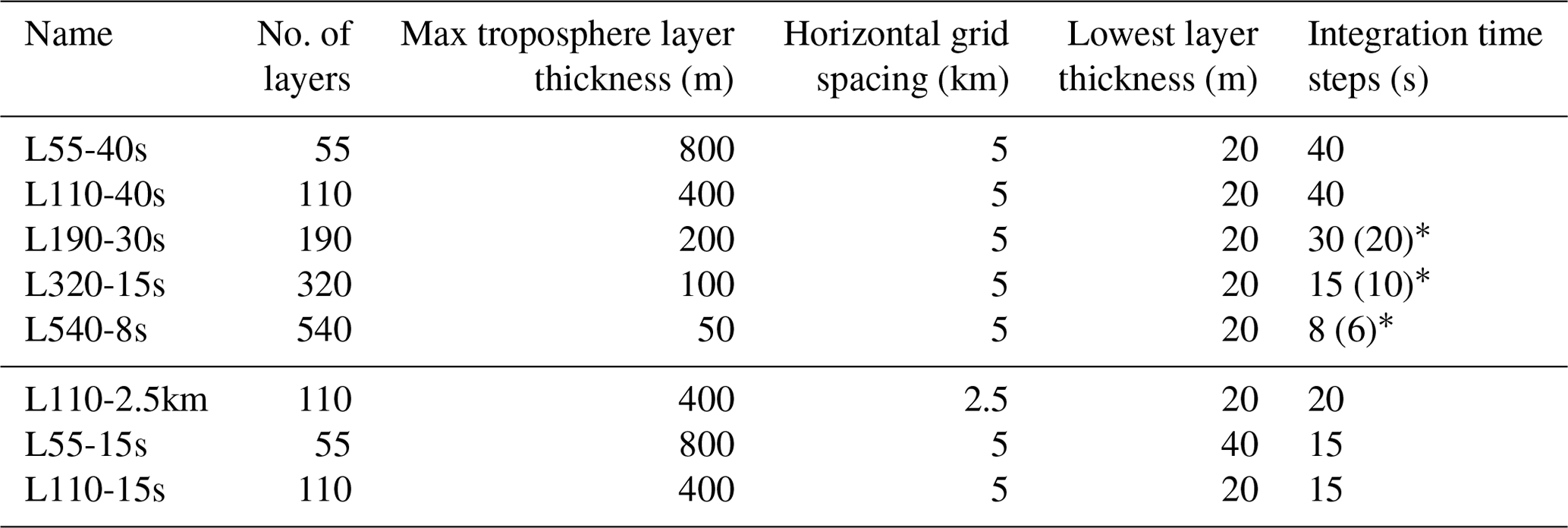
^* Time step lengths given in parentheses were used for few individual days of the simulations only, where the originally chosen time step caused instabilities.

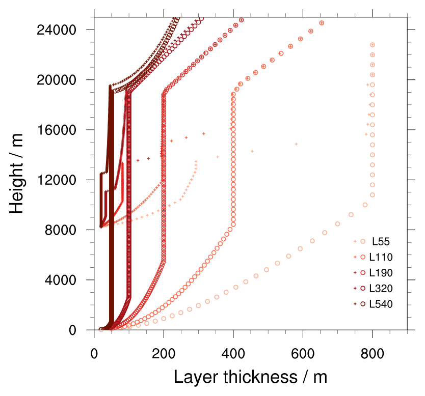
Figure 1 Vertical layer thickness for grid boxes with surface altitudes of 0 (circles) and 8205 m (crosses), respectively. The y axis shows the height of the lower edge of the respective layer. Colors indicate the experiments (see Table 1 for details), as shown in the legend. Darker colors mark finer vertical grid spacing. Only the lowest 25 km of the grids is shown. The model top is at 75 km for all configurations.

For the vertical discretization, all ICON atmosphere configurations employ the Smooth LEvel VErtical (SLEVE) coordinate (Leuenberger et al., 2010), a terrain-following hybrid sigma z coordinate. The decay of the effect of topography on the vertical coordinate is defined using functions described by Leuenberger et al. (2010). Parameters that define the grid for a specific configuration of ICON are, in particular, the minimum and maximum tropospheric layer thicknesses (Δz_min and Δz_max, respectively), where the minimum is used for the thickness of the lowest layer; the maximum altitude up to which these limits are applied (z_trop); and the altitude above which a fixed-height grid is used (z_fh).

To estimate the sensitivity of the simulated climate to the vertical grid spacing, we have performed five simulations with Δz_max values of 50, 100, 200, 400, and 800 m, corresponding to grids with between 540 and 55 layers in total. The first five lines of Table 1 show these simulations, which are all run at a horizontal grid spacing of about 5 km (measured as the square root of the triangle surfaces, called R2B9 following the terminology in Giorgetta et al., 2018) and with a model top at 75 km. Earlier storm-resolving ICON simulations, e.g., for the DYAMOND project, have often been performed with the same top height and Δz_max = 400 m but with only 90 vertical layers. Our reference grid L110 differs from this earlier vertical grid configuration in that z_trop is increased from 14 to 19 km in order to have well-defined layer thickness changes between the simulations for an altitude region that includes the tropical tropopause layer. Figure 1 shows layer thicknesses from the surface to 25 km altitude for the five vertical grids for surface altitudes of 0 and 8205 m. The latter corresponds to the grid box with the highest surface elevation of an R2B10 grid (with a horizontal grid spacing of about 2.5 km). Test simulations not further discussed in this paper revealed the tendency of the grids with 320 and 540 layers to frequently produce numerical instabilities. This issue could be solved by increasing the altitude where the grid is transitioning from a terrain-following to a fixed-height grid, which is why the three coarsest vertical resolutions are run with z_fh = 22 km, while we use values of 27 and 35 km for L320-15s and L540-8s, respectively. Attempts to use grids in which the spacing changes more smoothly with altitude than the grids presented in Fig. 1 did not reduce the instabilities.

Four further sensitivity simulations that have been performed are listed in Table 1. To put the effects of changes in vertical grid spacing into perspective, we have performed simulation L110-2.5km, which differs from the reference simulation L110-40s by its halved horizontal grid spacing and a halved integration time step. The standard simulations with different vertical (and horizontal) grid spacings use integration time steps of different lengths between 40 s (for L55-40s and L110-40s) and 8 s (for L540-8s). To disentangle the potential effects of changes in vertical and temporal discretization, we have performed two additional simulations, L55-15s and L110-15s, with configurations almost¹ identical to simulations L55-40s and L110-40s, respectively, but with a time step of 15 s, which is also employed in the L320-15s experiment. This creates a series of three experiments with an identical time step length but different vertical grid spacings. Simulations L55-15s and L110-15s have the additional benefit that differences in their respective references, L55-40s and L110-40s, can be unambiguously attributed to the different time steps.

The simulations in this study are initialized from the global meteorological analysis taken from the European Centre for Medium-Range Weather Forecasts (ECMWF) for 27 June 2021 at 00:00 UTC and are run for 45 d with daily sea surface temperature and sea ice fraction values taken from the ECMWF operational daily analyses as the lower boundary condition. Most comparisons of the climate state simulated in the different experiments are performed for the last 40 d of the simulation. Additionally, to enable some estimate of the internal variability in the simulations, four respective 10 d subperiods have been compared for parts of the analysis.

In the following sections, we will not only present the resolution dependencies of important climate quantities but also try to identify their causes. However, besides the plausible physical mechanisms, not easily identifiable numerical aspects in the individual remaining parameterizations or the interplay of parameterized and resolved phenomena may contribute. A thorough unit testing of the individual model components and their dependence on grid spacing and time step choices is arguably advisable to support the identification of the causes, but this is beyond the scope of this study. Nevertheless, the results presented here serve as a practical guide to understanding the large-scale effects and should be useful to the model development community.

3 Effects of vertical grid refinement

In most comparisons, we use the simulation L110-40s as a reference, because its vertical grid is closest to the standard configuration of ICON-Sapphire. In this section, we compare simulations with maximum tropospheric grid spacings reduced by up to a factor of 8 (L540-8s) with respect to this reference. The simulation with the coarsest vertical grid spacing (L55-40s) is presented separately in Sect. 4, as it behaves differently in several respects than one might extrapolate from the experiments with finer vertical grid spacing. Section 5 compares the effects of horizontal and vertical grid refinements. The first two subsections of this section report model results in terms of global means and horizontal patterns. The presentation of effects on vertical profiles in Sect. 3.3 is used to discuss potential reasons for the simulated effects. This discussion is continued in Sects. 4 and 5.

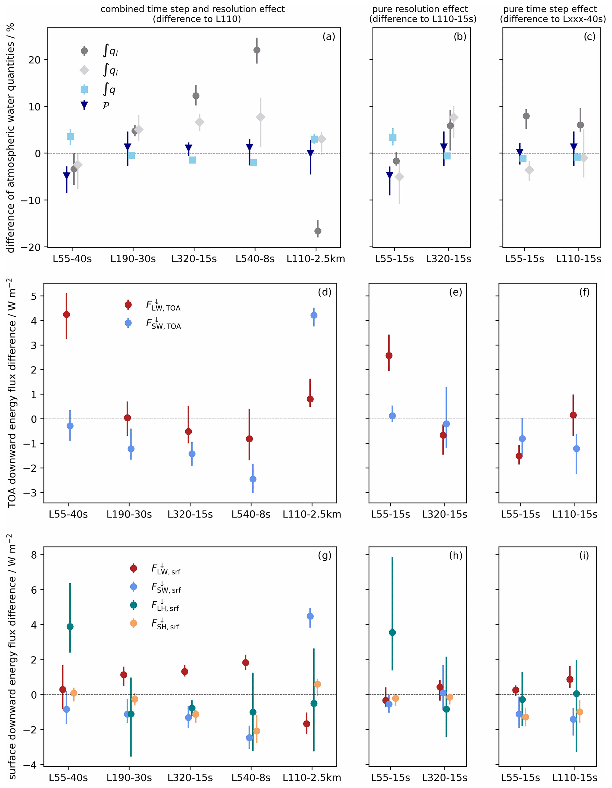
Figure 2 Panels (a), (d), and (g) show differences in the globally averaged atmospheric quantities from simulations that differ with respect to both the vertical grid spacing and the length of the integration time step, with the exception of L55-40s − L110-40s. Panels (b), (e), and (h) show the effects of differences in the vertical grid spacing only, while panels (c), (f), and (i) show the effects of differences in the time step only. Differences are calculated between the model configuration indicated on the x axis and (a, d, g) L110-40s, (b, e, h) L110-15s, and (c, f, i) the configuration with the same vertical grid spacing as the configuration on the x axis but a longer time step, respectively. Quantities depicted are vertically integrated cloud liquid water and cloud ice, precipitable water, and precipitation (∫q_l, ∫q_i, ∫q, 𝒫, respectively; a–c); net long-wave and short-wave radiation at the TOA ($F_{\mathrm{LW},\mathrm{TOA}}^{\downarrow }$ and $F_{\mathrm{SW},\mathrm{TOA}}^{\downarrow }$, respectively; d–f); and long-wave and short-wave radiation and sensible and latent heat fluxes at the surface ($F_{\mathrm{LW},\mathrm{srf}}^{\downarrow }$, $F_{\mathrm{SW},\mathrm{srf}}^{\downarrow }$, $F_{\mathrm{SH},\mathrm{srf}}^{\downarrow }$, and $F_{\mathrm{LH},\mathrm{srf}}^{\downarrow }$, respectively; g–i). All fluxes are defined positive downward. Markers depict the averages over 40 d, and the vertical bars mark the minimum and maximum differences in the four 10 d subperiods.

3.1 Global averages

3.1.1 Combined effects of vertical grid spacing and time step changes

When refining the spatial discretization of a numerical general circulation model, it is generally necessary to decrease the integration time step to ensure the stability of the integration by avoiding violation of the Courant–Friedrichs–Lewy (CFL) convergence condition. Therefore, we first discuss the effect of combined changes in the vertical grid spacing and the integration time step for the first five experiments listed in Table 1. For simplicity, we refer to these combined changes as “practical vertical resolution changes”, as the goal is to change the vertical grid spacing, while the time step is only changed out of necessity. The individual effects of grid spacing and time step changes will be presented in Sect. 3.1.2.

Figure 2a shows differences in the global mean precipitation, precipitable water, and vertically integrated cloud ice and liquid water of experiments L190-30s, L320-15s, and L540-8s, with each compared to the reference experiment L110-40s. Experiments L55-40s and L110-2.5km are included in this figure but will be discussed in the following sections.

Precipitation differences among the experiments are small and, as indicated by the vertical bars, can be of different sign for different 10 d subperiods within the same experiment. Possibly, 10 d simulation periods are too short to unambiguously represent a potential effect of vertical grid spacing on precipitation. Over longer time spans, precipitation is constrained by the atmospheric energy balance (e.g., Mitchell et al., 1987; Fläschner et al., 2016). Summing up the radiation fluxes of Fig. 2d and g indicates increases in atmospheric radiative cooling of between about 1 W m⁻² for the practical refinement in L190-30s and 3 W m⁻² for the practical refinement in L540-8s. These increases are largely balanced by the turbulent energy fluxes at the surface and, hence, consistent with small increases in precipitation. The energy fluxes will be discussed in more detail below. Precipitable water decreases with practical increases in the vertical resolution. The difference between L540-8s and L110-40s is about 2 %.

A large dependence on a practical vertical grid refinement is simulated for vertically integrated cloud liquid water, which increases by similar amounts for each halving of grid spacing. The effect reaches about 22 % for the reduction in the maximum tropospheric grid spacing from 400 m in L110-40s to 50 m in L540-8s. Convergence is not observable within the range of grid spacings used here. Vertically integrated cloud ice also increases with vertical resolution, but the effect is smaller than for liquid water. The L190-30s, L320-15s, and L540-8s experiments show respective increases in vertically integrated cloud ice of about 5 %, 7 %, and 8 % compared with L110-40s, indicating convergence for this quantity.

The effects on the global mean vertical energy fluxes at the TOA and the surface are shown in Fig. 2d and g, respectively. Net downward TOA shortwave radiation decreases with practical increases in the vertical resolution (by about 2.5 W m⁻² for L540-8s compared with L110-40s), as may be expected from the increase in cloud water. Outgoing longwave radiation (OLR) seems to increase with practical increases in the vertical resolution, although the spread between the individual 10 d periods is large.² From the increase in cloud ice, one would expect the opposite behavior a priori, but the sign is consistent with the reduction in precipitable water. The apparent inconsistency in the cloud ice and longwave radiation effects will be discussed in Sect. 3.3.

The effects on the net shortwave downward radiation at the surface are similar to its TOA component for all experiments. Net surface downward longwave radiation increases with practical increases in the vertical resolution, which would be consistent with more cloud liquid water and ice. The upward sensible heat flux increases with practical increases in the vertical resolution, as also seems to be the case for the latent heat flux. The latter signal is very variable and may not be robust, but it is consistent with the increasing atmospheric radiative cooling mentioned above.

In summary, the individual components of the TOA and surface energy fluxes presented in Fig. 2 respond very differently in magnitude to practical changes in the vertical resolution, but none of them show a clear tendency toward convergence for the range of vertical grid spacings tested here.

Hohenegger et al. (2020) compared the effects of their horizontal resolution changes in ICON to the multi-model standard deviation of the DYAMOND model intercomparison project. In terms of global means, they concluded that simulated differences between horizontal grid spacings of 2.5 and 5 km are small in comparison to the multi-model spread. As we will show in Sect. 5, the effects of halving the vertical grid spacing are generally smaller than those of halving the horizontal grid spacing. Hence, the effects of practical vertical resolution doubling are also small with respect to this metric.

In the following, we will first analyze the degree to which the reported changes in selected global mean climate quantities are due to changes in the spatial resolution or time step length. Following this, we will analyze horizontal and vertical patterns of the changes to better understand the origin of global mean effects. The focus will be on the robust signals in both cloud condensate components and their effects on radiative fluxes.

3.1.2 Individual effects of vertical grid spacing and time step changes

Figure 2b, e, and h show differences in the same quantities discussed above for experiments L320-15s to L110-15s. These two experiments use the same integration time step of 15 s (except for a single day for L320-15s that was run with 10 s to overcome an instability) but differ with respect to their vertical grid spacing. Figure 2c, f, and i show differences in experiments L110-15s and L110-40s and in experiments L55-15s and L55-40s, i.e., the effects of a pure reduction in the integration time step from 40 to 15 s.

Comparison of Fig. 2a, b, and c indicates that the increase in the cloud liquid water is due to both the changing vertical resolution and time step. Both changes appear to contribute about equally to the total effect, although the exact contributions are uncertain due to temporal variability. While the maximum tropospheric vertical grid spacing is reduced to one-quarter of the L110-40s value in L320-15s, the time step is only reduced to three-eighths of the L110-40s value.

An increase in cloud liquid water would be consistent with an increase in the reflected shortwave radiation, as mentioned above. However, the previously discussed reduction in the TOA downward shortwave radiation with increasing vertical resolution seems to be largely a time step effect, while the pure resolution effect is small.

In contrast to cloud liquid water, the effect on the vertically integrated cloud ice reported above is dominantly indeed a vertical resolution dependence. The reported effect on the sensible heat flux, on the other hand, is largely a time step effect.

The global net radiative effect of a practical vertical resolution increase is a cooling. In experiment L320-15s, e.g., in comparison to L110-40s, the global total net downward energy fluxes at both the TOA and surface are about 1.9 W m⁻² smaller. Both effects are dominated by the time step dependence. The origin of this will be discussed below.

3.2 Spatial distributions

Figure 3 shows the zonal mean differences in the selected cloud and radiation flux quantities between selected simulations. To facilitate the identification of signals, we do not present the results from all practical vertical refinement experiments, leaving out experiment L190-30s, which causes similar but weaker signals than the grids with even finer resolution, and limit ourselves to the L320-15s − L110-15s difference for the pure resolution effect and the L110-15s − L110-40s difference for the pure time step effect. The zonal mean L320-15s − L110-40s and L540-8s − L110-40s differences show similar latitude dependence for all presented quantities, with generally larger amplitudes for the latter difference. This increases our confidence in the robustness of these signals.

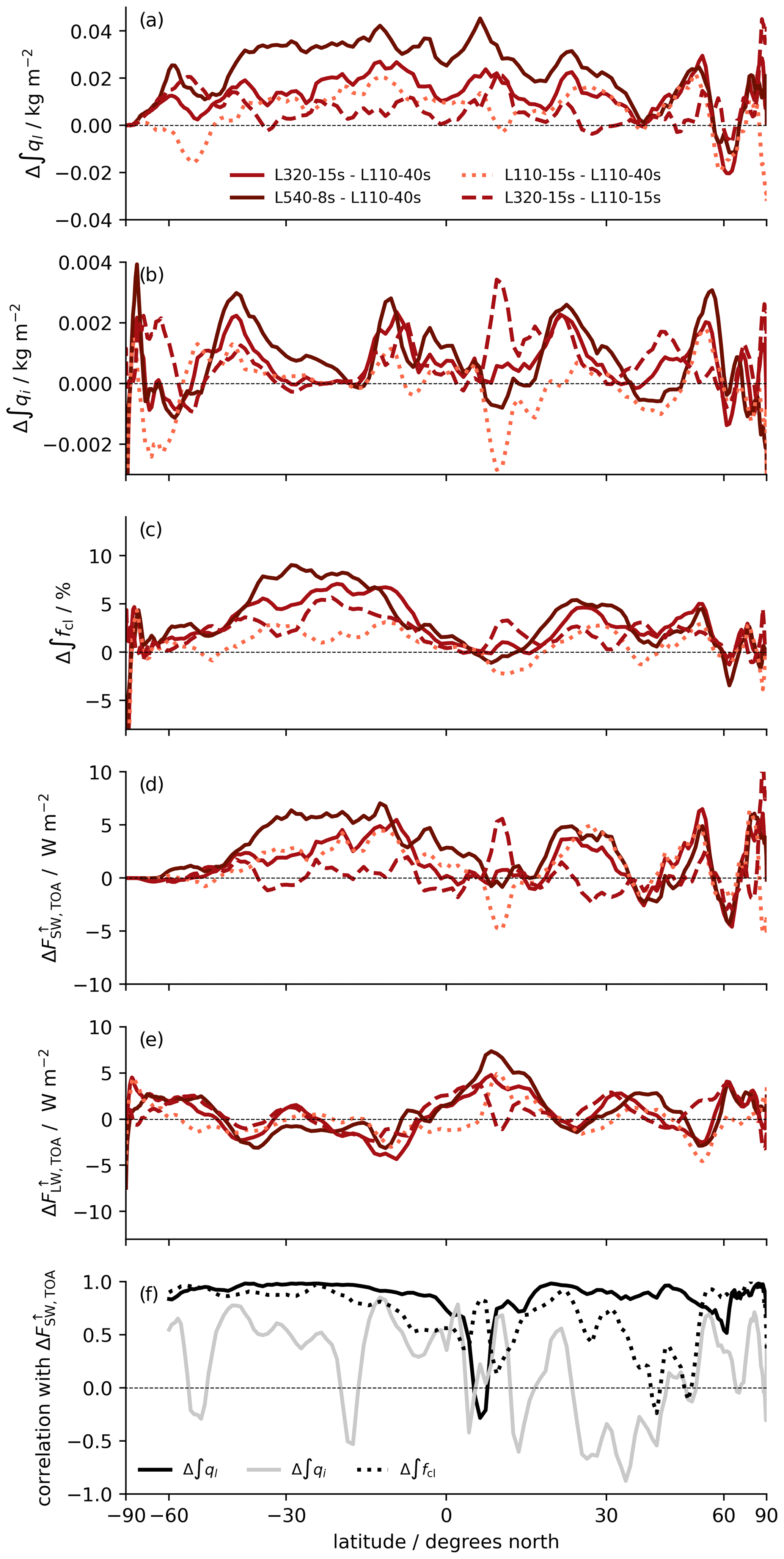
Figure 3 Panels (a) to (e) show differences in the zonally averaged atmospheric quantities between simulations, as indicated in the legend of panel (a). The quantities are (a) vertically integrated cloud liquid water (∫q_l), (b) vertically integrated cloud ice (∫q_i), (c) total cloud fraction (∫f_cl), (d) outgoing shortwave radiation at TOA ($F_{\mathrm{SW},\mathrm{TOA}}^{\uparrow }$), and (e) outgoing longwave radiation at TOA ($F_{\mathrm{LW},\mathrm{TOA}}^{\uparrow }$). Solid lines mark differences in the practical vertical resolution changes (i.e., generally also including a time step change), the dashed line denotes a difference caused by a pure vertical resolution change, and the dotted line marks a difference caused by a pure time step change. All quantities are averaged over the last 40 d of the simulations. Panel (f) shows coefficients of correlations of $F_{\mathrm{SW},\mathrm{TOA}}^{\uparrow }$ with ∫q_l, ∫q_i, and ∫f_cl, respectively, calculated for each latitude and all of the experiments in Table 1.

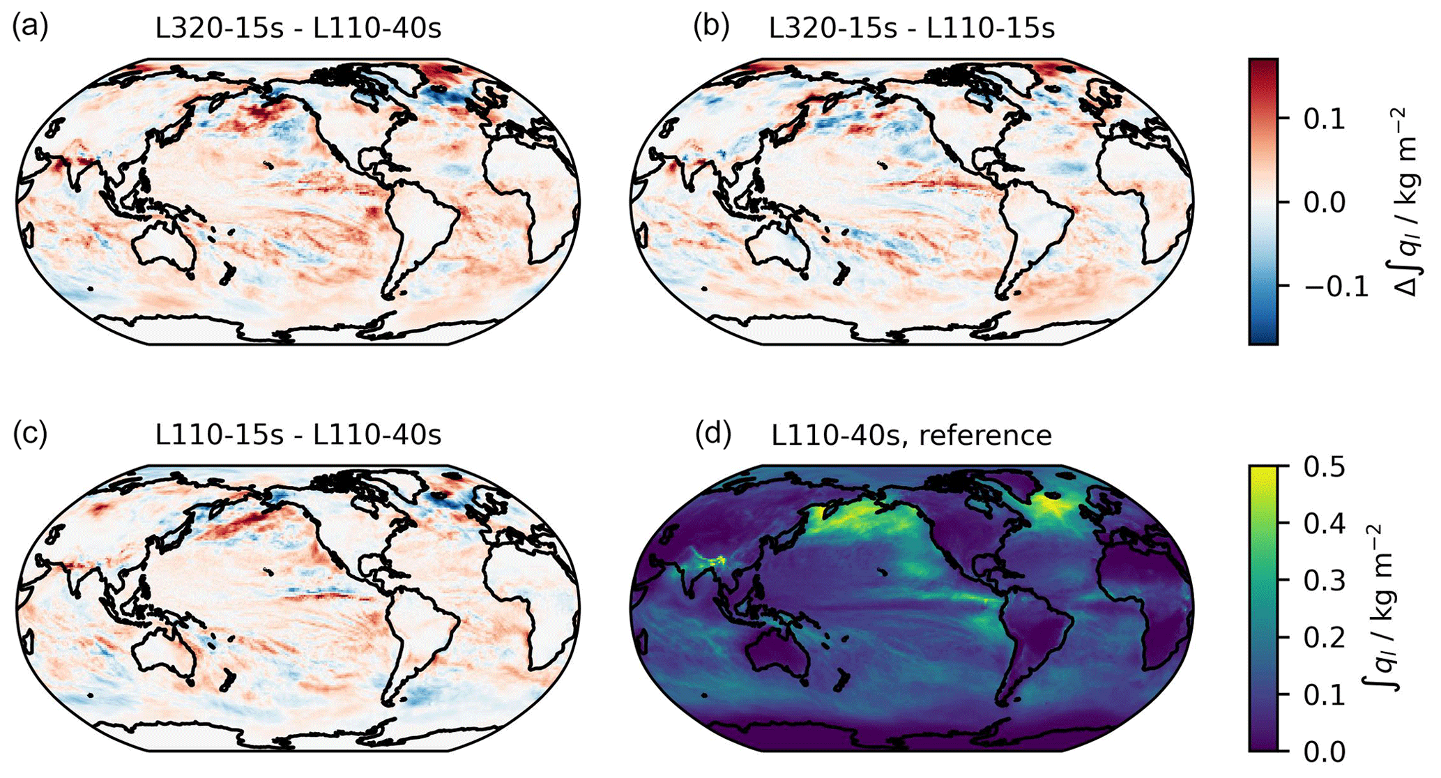
Figure 4 Vertically integrated cloud liquid water (kg m⁻²) from (d) simulation L110-40s and (a–c) differences in this quantity between the simulations indicated in the panel titles. All quantities are averaged over the last 40 d of the simulations.

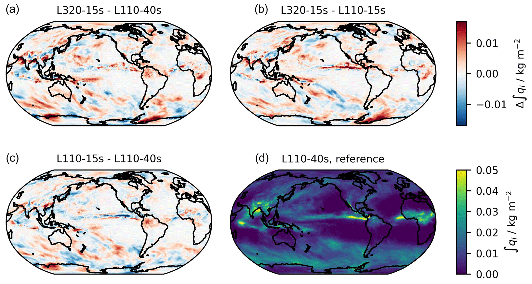
Figure 5 Vertically integrated cloud ice (kg m⁻²) from (d) simulation L110-40s and (a–c) differences in this quantity between the simulations indicated in the panel titles. All quantities are averaged over the last 40 d of the simulations.

Figure3a indicates that the global increase in the vertically integrated cloud liquid water with a practical increase in the vertical resolution is due to increases over a large latitude range from the southern to northern midlatitudes. As for the global mean differences, there is also no tendency toward convergence with higher resolution over this entire latitude range. Despite some variability, the curves also confirm that the pure time step effect (L110-15s − L110-40s) has a larger contribution than the pure vertical resolution effect (L320-15s − L110-15s) to the practical resolution effect (L320-15s − L110-40s). While there also appears to be a distinct pattern at higher, in particular northern, latitudes, this pattern is much more dependent on the averaging period than the effects at lower latitudes and may depend strongly on the accidental evolution of the meteorological situation in the different simulations. Therefore, in the analysis of the vertical structure of resolution change effects (Sect. 3.3), we will concentrate on tropical (30^∘ S–30^∘ N) averages. The difference maps in Fig. 4 confirm that the increase in cloud liquid water is widespread over middle- to low-latitude oceans and that both the time step and the vertical grid spacing contribute to this effect. Based on past studies with LES models (e.g., Marchand and Ackerman, 2011) or GCMs (e.g., Bogenschutz et al., 2021), one may expect that in particular the amount of liquid water in stratocumulus areas increases with finer vertical grid spacing. A better-resolved inversion may reduce the ventilation of the boundary layer or, in other words, the mixing of moist boundary layer air into the free troposphere. Indeed, the patterns of the L320-15s − L110-40s difference shown in Fig. 4 and of the L540-8s − L110-40s difference (not shown) indicate a relatively strong increase off the west coast of northern South America, but this signal certainly does not dominate the zonal mean and is not visible in other stratocumulus regions, such as off the west coast of North America. Furthermore, it seems again that the time step effect, as indicated by the L110-15s − L110-40s difference, contributes strongly to the signals seen in the L320-15s − L110-40s difference. Interestingly, the aforementioned studies of Bogenschutz et al. (2021) and Lee et al. (2022) also noted that the South American stratocumulus region is particularly sensitive to vertical resolution changes.

The latitudinal distribution of the increase in vertically integrated cloud ice (Fig. 3 b) is much less uniform than that of liquid water, and the same is true for the spatial pattern shown in Fig. 5. While this cannot be easily identified from the map, it will be shown (in Sect. 3.3.2) that the signal differs on average between moist and dry regions of the tropics. In the zonal mean, pure and practical increases in the vertical resolution lead to increases in the zonal mean cloud ice amount with peaks near 40 and 10^∘ S and near 20 and 50^∘ N. The degree to which these peaks are due to the accidental evolution of weather in the individual experiments or are actually a signal of the resolution differences is unclear. Zonal average differences calculated for the first 5 d of the simulation period (not shown), for which the meteorology is still fairly similar among the simulations, indicate more uniform increases for finer vertical grid spacings, in particular very similar effects of the practical increase to 320 layers and the pure effect of such a resolution increase. This confirms that the ice signal is, contrary to the liquid water signal, largely unaffected by the time step differences. In contrast, the local increase in cloud ice over northern South America with a practical resolution increase is mostly a time step effect.

The effect of an increasing vertical resolution on cloud liquid water is strongly correlated with the effect on zonal mean outgoing, i.e., reflected, shortwave radiation (solid black line of Fig. 3f) and anticorrelated with net surface shortwave radiation (not shown). Regional maxima of an increase in shortwave reflection are, for example, simulated in the abovementioned stratocumulus region off South America, with values of up to about 30 W m⁻² for the L540-8s − L110-40s comparison. The correlation breaks down near the intertropical convergence zone (ITCZ), which is centered slightly north of the Equator during the simulation period and where no increase in the outgoing shortwave reflection is simulated despite increases in cloud liquid water. Here, the reflected shortwave radiation is also not strongly correlated with vertically integrated cloud ice but rather with the cloud fraction (solid gray and dotted black lines in Fig. 3f, respectively). In Sect. 3.3.2, the fact that vertically integrated cloud ice and cloud fraction may be anticorrelated in some areas will be discussed.

3.3 Vertical profiles

3.3.1 The boundary layer

We have mentioned above that vertically integrated cloud liquid water increases over a large latitude range, dominantly due to a reduction in the time step but additionally due to an increase in vertical resolution. Figure 6 shows the vertical profile of cloud liquid water averaged over 30^∘ S–30^∘ N and the differences in this quantity due to individual and combined changes in the grid spacing and integration time step. It is clear that the different changes have distinct effects on the profile.

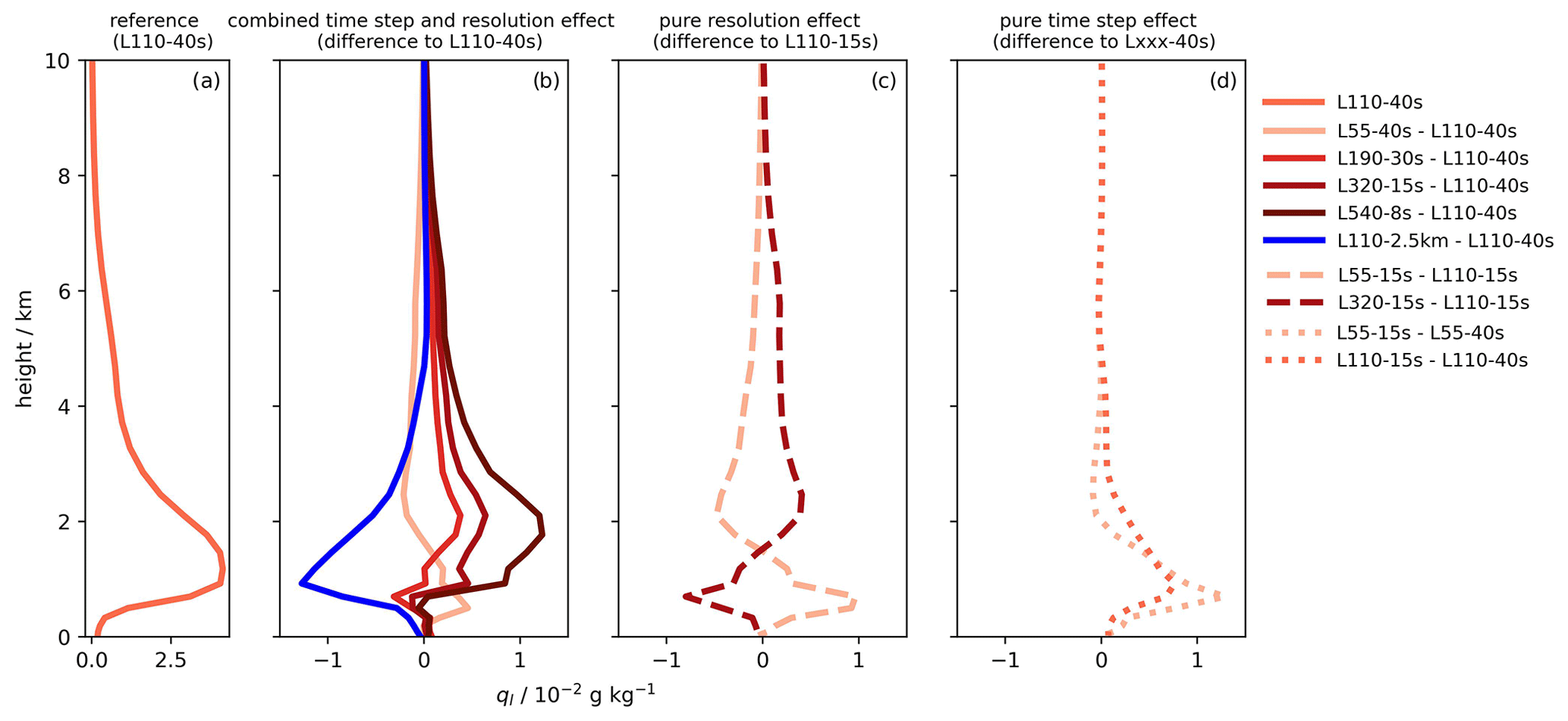
Figure 6 Vertical profiles of the cloud liquid water concentration (10⁻² g kg⁻¹) averaged over the tropics (30^∘ S–30^∘ N) from (a) simulation L110-40s and the effects on this quantity resulting from (b) combined vertical resolution and time step changes, (c) pure vertical resolution changes, and (d) pure time step changes. Profiles in panel (b) are calculated as the differences between the simulation indicated in the legend and simulation L110-40s, panel (c) shows differences between the simulation indicated in the legend and simulation L110-15s, and panel (d) shows the differences for L55-15s − L55-40s and L110-15s − L110-40s. To compare the different grids, all values have been interpolated to the L55 grid.

A shorter time step increases the liquid water content in the cloud layer, dominantly near the lifting condensation level. A higher vertical resolution shifts the profile upwards. While time step and resolution effects are not necessarily independent of each other (see Sect. 4), the effect of a practical vertical resolution increase is generally well approximated by a combination of the two individual effects. It is clear from Fig. 6 that the effect of increased vertical resolution on cloud liquid water is not converging in the range of vertical resolutions used in these experiments.

The origin of the increase in cloud liquid water for a practical increase in the vertical resolution is not easy to identify. Using the same GCM, Bogenschutz et al. (2021) and Wan et al. (2021) also recognized a strong time step sensitivity of low clouds. However, in their model, which uses convection parameterizations, the low-cloud fraction decreases with a shorter time step. Wan et al. (2021) show that this sensitivity depends on the specifics of the numerical coupling of various processes in the model integration, in particular the parameterizations of convection and cloud micro- and macrophysics.

Concerning the effect of a spatial refinement on cloud condensate, one may assume that there is simply a larger chance to reach saturation when splitting a grid box in two. While we cannot exclude such an effect, other processes seem to dominate, as a refinement in the vertical grid produces an altitude shift and a refinement in the horizontal grid even produces a reduction in cloud liquid water (see Sect. 5).

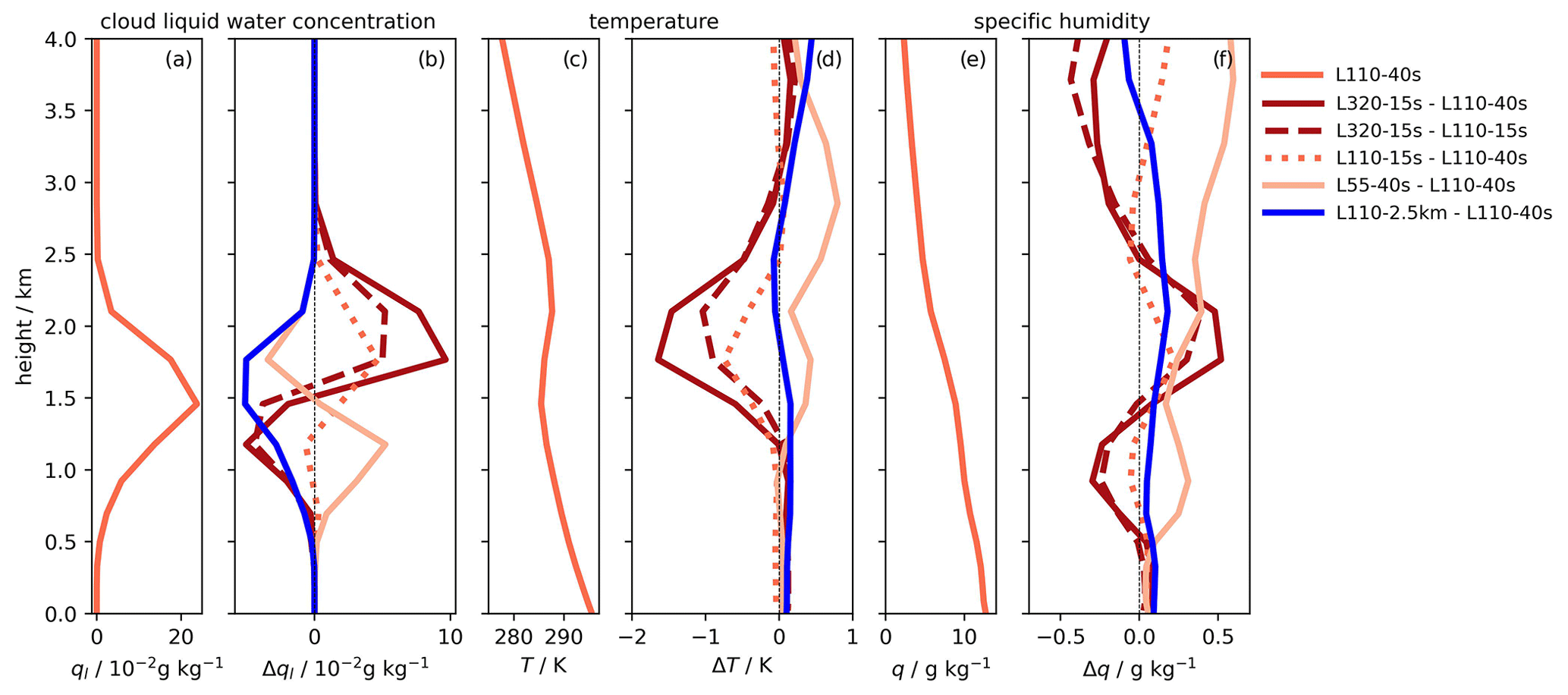
Figure 7 Vertical profiles of (a) cloud liquid water concentration (q_l, 10⁻² g kg⁻¹), (c) temperature (T, K), and (e) specific humidity (q, g kg⁻¹) from L110-40s averaged over the region from 15^∘ S to 0^∘ N and from 105 to 90^∘ W, i.e., a stratocumulus region off the South American coast. Panels (b), (d), and (f) show the differences in the respective quantities for a practical increase in the vertical resolution (L320-15s − L110-40s; solid dark red), a pure increase in the vertical resolution (L320-15s − L110-15s; dashed dark red), a pure time step decrease (L110-15s − L110-40s; dotted red), a decrease in the vertical resolution (L55-40s − L110-40s; solid light red), and a practical increase in the horizontal resolution (L110-2.5km − L110-40s; solid blue).

To better understand the effects, we will have a closer look at marine stratocumulus off the coast of South America, where signals are strong (Fig. 4). As mentioned earlier, an increase in cloud liquid water in the marine stratocumulus regions may be expected for a finer vertical grid spacing due to a potentially better inversion layer resolution, and this is also simulated in our experiments. Figure 7 shows vertical profiles of cloud liquid water, temperature, and specific humidity averaged over the region from 15^∘ S to 0^∘ N and from 105 to 90^∘ W. The profiles support the interpretation of a deepening boundary layer and an upward-shifting cloud layer for finer vertical grid spacing (Fig. 7b). The upward shift in the inversion can be seen in the temperature profile that shows a reduction of almost 2 K near 1.8 km when comparing L320-15s and L110-40s. The profiles of cloud liquid water, specific humidity, and relative humidity (not shown) all show a strong reduction near the reference cloud base and a strong increase near the reference cloud top. Apparently, the better representation of the inversion leads to a deepening of the boundary layer and also a drying of the free troposphere (see Fig. 7f).

In this stratocumulus region, the individual effects of vertical resolution and time step changes are less shifted against each other in altitude than over the average tropics, and both effects contribute to the liquid water increase near the reference cloud top. The overall increase is mainly due to the time step effect, as it is basically positive all over the cloud layer, while the pure resolution effect is a vertical shift. However, in contrast to the tropical average, the simulated changes in the reference do not increase much when going to even finer grid spacings than in L190-30s (not shown). This occurs despite the experience from LESs of a large sensitivity to changes in vertical grid spacings even at much smaller scales than those considered in our simulations (e.g., Marchand and Ackerman, 2011; Mellado et al., 2018).

An increase in the stratocumulus cloud amount was also simulated in a GCM by Bogenschutz et al. (2021) for an up to 8-fold increase in the number of vertical levels in the boundary layer. However, as in our case, the boundary layer depth only increased for the first two 2-fold changes. The last doubling led to a decrease in the depth. Moreover, in their case, a shorter integration time step led to a reduction in the cloud amount.

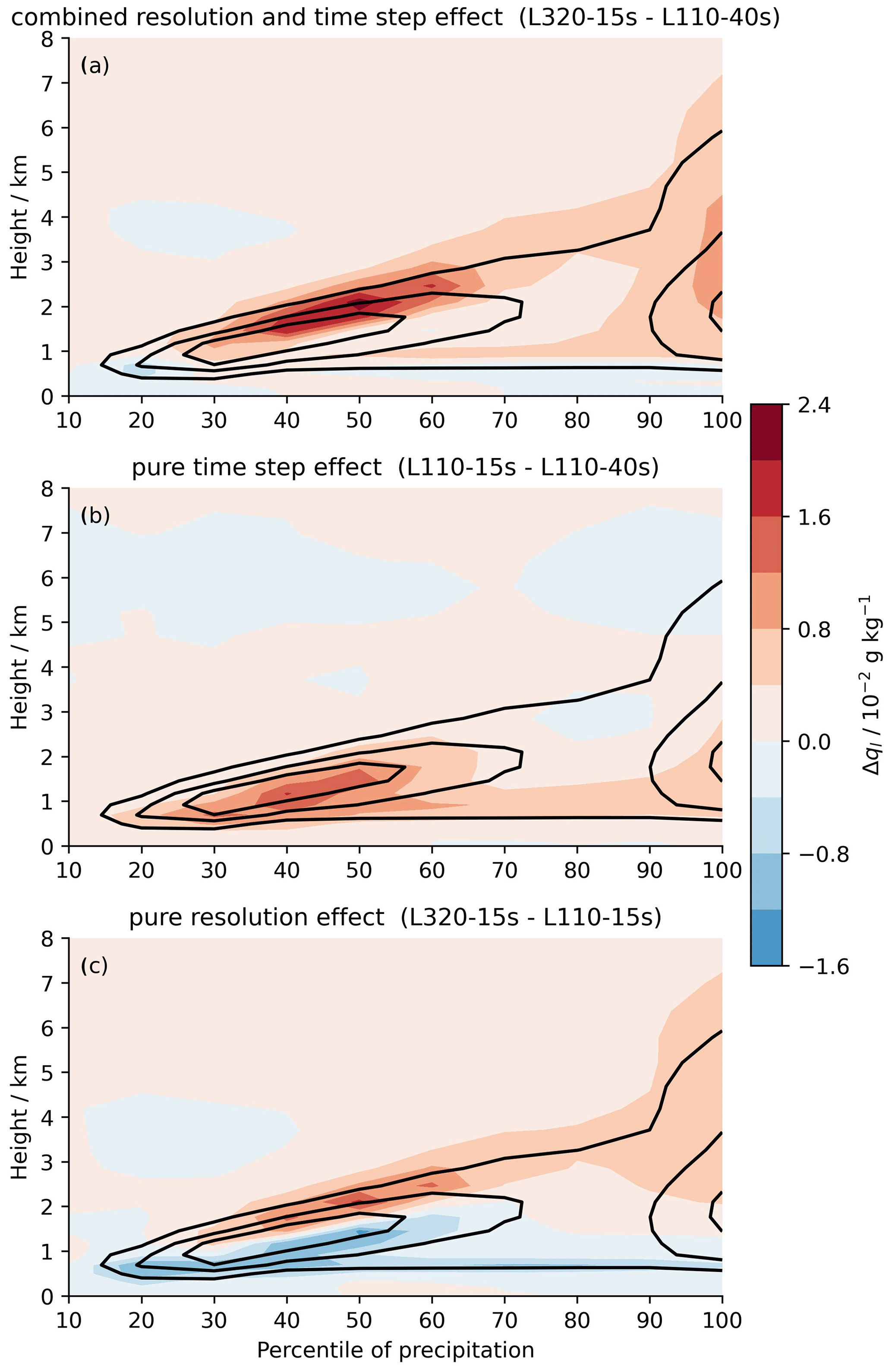
Figure 8 Color shading indicates the difference in the vertical profiles of the cloud liquid water concentration (q_l) between experiments (a) L320-15s − L110-40s, (b) L110-15s − L110-15s, and (c) L320-15s − L110-15s averaged over percentile bins of tropical precipitation. Numbers on the x axis mark the percentiles: 10, for example, marks the mean profile for the tropical 1^∘ × 1^∘ areas and simulated days with the 10 % lowest precipitation rates, whereas 100 marks the 10 % highest precipitation rates. Black solid lines mark average q_l values of 2 × 10⁻², 4 × 10⁻², and 6 × 10⁻² g kg⁻¹ in L110-40s.

While the effects of resolution changes in the selected stratocumulus region are much larger than in the tropical average, there are a lot of qualitative similarities which suggest that similar mechanisms are in play all over the tropics. This widespread occurrence of similar changes is confirmed by Fig. 8, which shows changes in the tropical vertical profiles of cloud liquid water in precipitation space. The upward shift caused by the finer grid spacing and the increase in cloud liquid water that dominantly occurs in the lower part of the cloud layer for a shorter time step is happening in most precipitation regimes.

Resolution effects on the vertical profiles of cloud liquid water averaged over southern and northern midlatitudes (not shown) are qualitatively similar to the tropics, despite relatively large regional variations, in particular in the Northern Hemisphere (Fig. 4). We speculate that reduced ventilation of the boundary layer and possibly also reduction in the numerical diffusion through the refinement in the grid contribute to the changes in cloud liquid water simulated over a variety of different conditions.

3.3.2 The free troposphere

We reported above that vertically integrated cloud ice is hardly affected by changes in the integration time step; rather, it is almost only impacted by the pure changes in the vertical grid spacing. Figure 9 shows that refining the grid spacing basically increases tropical cloud ice at all altitudes at which it also exists in the reference simulation. The largest absolute increase is simulated near the cloud ice peak at around 11 km. Only near 14 km is cloud ice slightly reduced for finer vertical grid spacing. Figure 9 also confirms the earlier notion that the effect of refining the grid spacing seems to converge for the highest resolution used in our simulations.

Figure 9 Same as Fig. 6 but for the cloud ice concentration (10⁻⁴ g kg⁻¹).

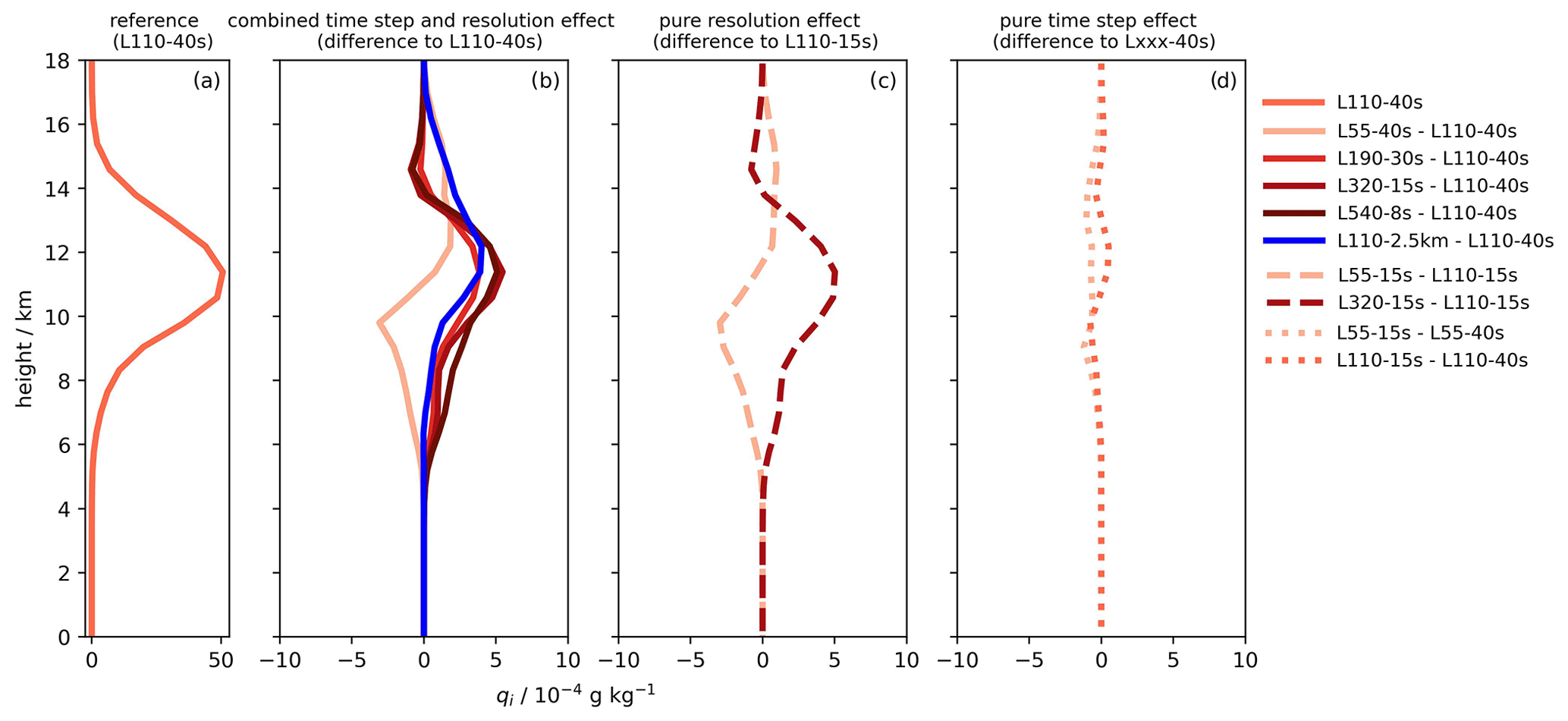
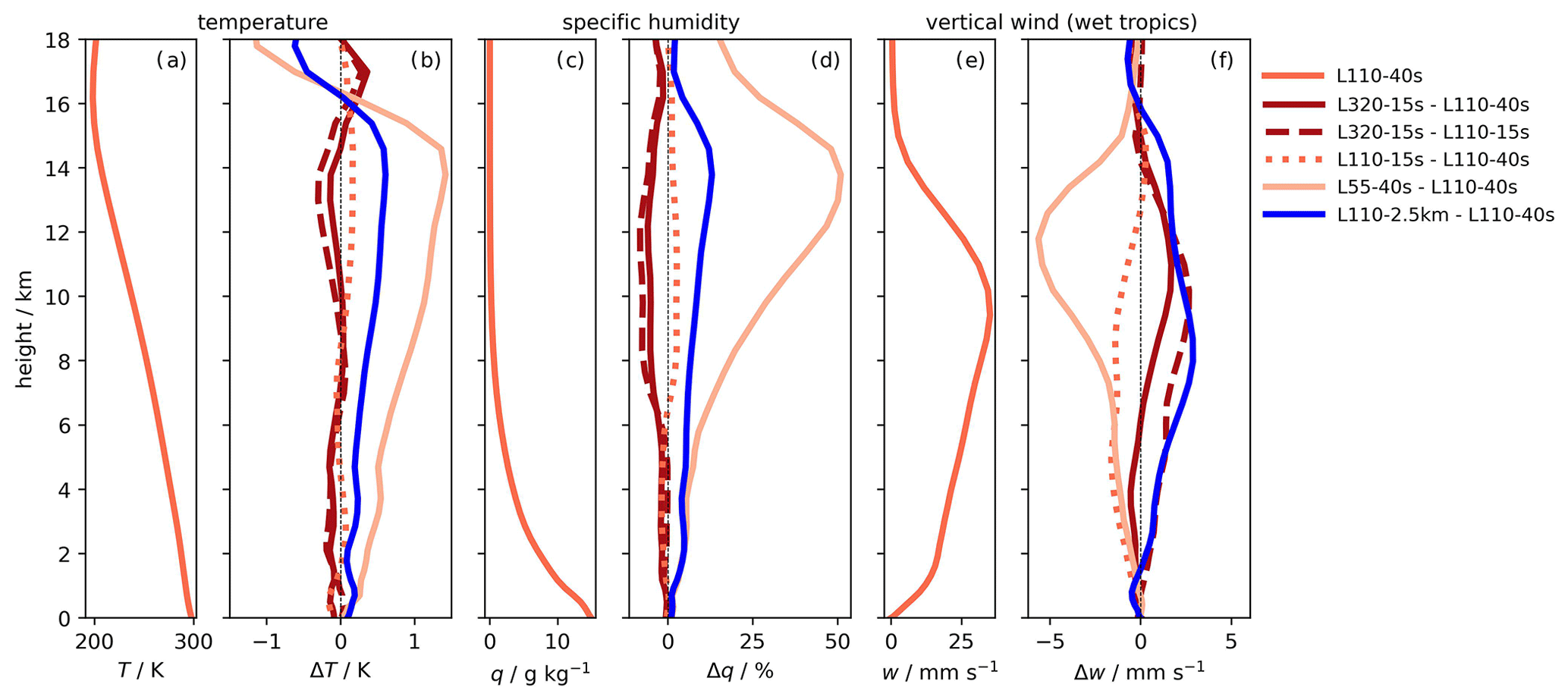
Figure 10 Vertical profiles of (a) temperature (T, K), (c) specific humidity (q, g kg⁻¹), and (e) vertical wind (w, m s⁻¹) from L110-40s averaged over the tropics (30^∘ S–30^∘ N); for the vertical wind, data are averaged over the 10 % of the tropical area with the highest precipitation. Panels (b), (d), and (f) show the differences in the respective quantities for a practical increase in the vertical resolution (L320-15s − L110-40s; solid dark red), a pure increase in the vertical resolution (L320-15s − L110-15s; dashed dark red), a pure time step decrease (L110-15s − L110-40s; dotted red), a decrease in the vertical resolution (L55-40s − L110-40s; solid light red), and a practical increase in the horizontal resolution (L110-2.5km − L110-40s; solid blue).

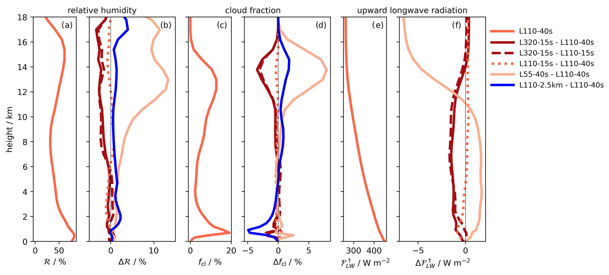
Figure 11 Same as Fig. 10 but for the tropical averages of (a) relative humidity (ℛ, %), (c) cloud fraction (f_cl, %), and (e) upward longwave radiation flux (${\mathcal{F}}_{\mathrm{LW}}^{\uparrow }$, W m⁻²). Differences in the relative humidity and cloud fraction are given in percentage points. Due to limited model output radiation, fluxes are averaged over 30 d only (instead of the 40 d used for all other time averages) and are not given for L110-2.5km.

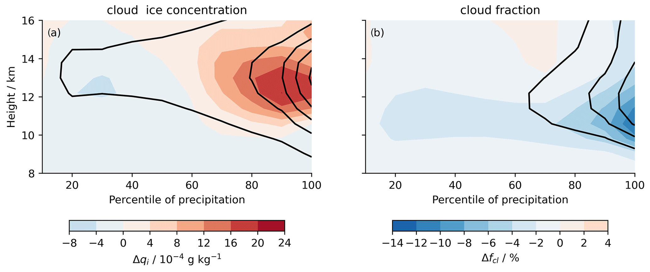
Figure 12 (a) Color shading indicates the difference in the vertical profiles of the cloud ice concentration (q_i) between experiments L540-8s and L110-40s averaged over percentile bins of tropical precipitation. Numbers on the x axis mark the percentiles: 10, for example, marks the mean profile for the tropical 1^∘ × 1^∘ areas and simulated days with the 10 % lowest precipitation rates, whereas 100 marks the 10 % highest precipitation rates. Black solid lines mark average q_i values of 10, 60, 110, 160, and 210 × 10⁻⁶ g kg⁻¹ in L110-40s. Panel (b) is the same as panel (a) but for the cloud fraction f_cl (in %). Black isolines mark average f_cl values of 10 %, 20 %, and 30 %.

To better understand possible causes and consequences of this change in cloud ice, Figs. 10 and 11 show tropical mean vertical reference (L110-40s) profiles of temperature, specific humidity, vertical wind, relative humidity, cloud fraction, and upward longwave radiation as well as the respective differences in these quantities for selected experiments. As an indicator of convective activity, the vertical wind velocity is not averaged over the whole tropics but rather over the 10 % of the tropical area with the strongest precipitation for a given time interval.³

Cloud ice increases with a refinement in the vertical grid (Fig. 9c), although specific humidity (Fig. 10d) and, despite the lower temperature (Fig. 10b), relative humidity (Fig. 11b) are reduced at almost all altitudes at which cloud ice exists.

Figure 12a shows tropical cloud ice profiles in precipitation space and their differences between experiments L540-8s and L110-40s.⁴ The average increase in cloud ice is dominated by the regions with high precipitation, i.e., the regions in which deep convection occurs. In tropical regions with low precipitation, the vertically integrated ice cloud content (not shown) decreases by about 20 %. This means that the changes in relative humidity and cloud ice in these regions are consistent. However, this is not the case in regions with high precipitation. In these latter regions, the increase in cloud ice is likely related to the increase in upwelling (Fig. 10f) transporting more condensate upwards.

The increase in the upwelling is consistent with the drying of the troposphere, visible in both specific and relative humidity (Figs. 10d and 11b), which increases atmospheric radiative cooling (not shown) that needs to be balanced by stronger subsidence in the dry tropical regions. The effect on the atmospheric moisture will be discussed in the following section, as it is particularly strong for a coarsening of the vertical grid. The change in upwelling in the moist tropics is also consistent with the temperature changes. A pure time step decrease (L110-15s − L110-40s) reduces temperatures in the boundary layer and convective upwelling. A pure vertical resolution increase (L320 − L110-15s) decreases temperature over almost all of the tropical profile above the boundary layer, thereby increasing the convective available potential energy and upwelling. This results in an almost unchanged upwelling up to about 8 km and an increase up to about 14 km for the practical increase in the vertical resolution (L320-15s − L110-40s).

Figure 12b shows that the cloud fraction is reduced everywhere in precipitation space at tropical ice cloud altitudes, despite the increase in the cloud ice content in high precipitation areas. Thus, the opposing signals in the cloud ice concentration and cloud fraction (Figs. 9 and 11d) are dominated by the changes in the areas of high precipitation, not by the subsidence regions where the changes have the same sign. ICON-Sapphire uses a cloud scheme that sets the cloud fraction in individual grid boxes to 1 if the total condensate concentration is above the threshold of 10⁻³ g kg⁻¹ or to 0 otherwise. Thus, a lower average cloud fraction means that fewer grid boxes are filled with a sufficient condensate mixing ratio. The apparent contradiction between a lower cloud fraction and a higher cloud ice concentration at some altitudes can only be explained by a larger concentration in fewer condensate-filled grid boxes. This would be consistent with the distribution of lower supersaturation over larger grid boxes suggested by Seiki et al. (2015) for coarser vertical grid spacing. They argued that finer vertical grid spacing would accelerate the interaction between clouds and radiation due to smaller air mass in a cloudy grid box and, hence, faster temperature change. Increased cloud top cooling in such boxes would decrease stability and increase the variability in supersaturation. However, it is not clear if this is the dominant process in our simulations. Consistent with our results, Ohno et al. (2019) also simulate a reduction in the high-cloud fraction for finer vertical grids in RCE simulations with NICAM at a 28 km horizontal resolution.

4 Effects of vertical grid coarsening

Figure 2 shows that many global mean quantities change more strongly when coarsening the vertical grid with respect to the reference (L55-40s − L110-40s) than when refining it. For instance, in the case of precipitation, the L55-40s − L110-40s and L55-15s − L110-15s differences are the only signals for which the spread between the four individual 10 d periods does not include zero. Both differences result purely from the change in vertical grid spacing, as the compared simulations use identical time steps of 40 and 15 s, respectively. The similarity in the L55-40s − L110-40s and L55-15s − L110-15s differences provides confidence in the robustness of the signals.

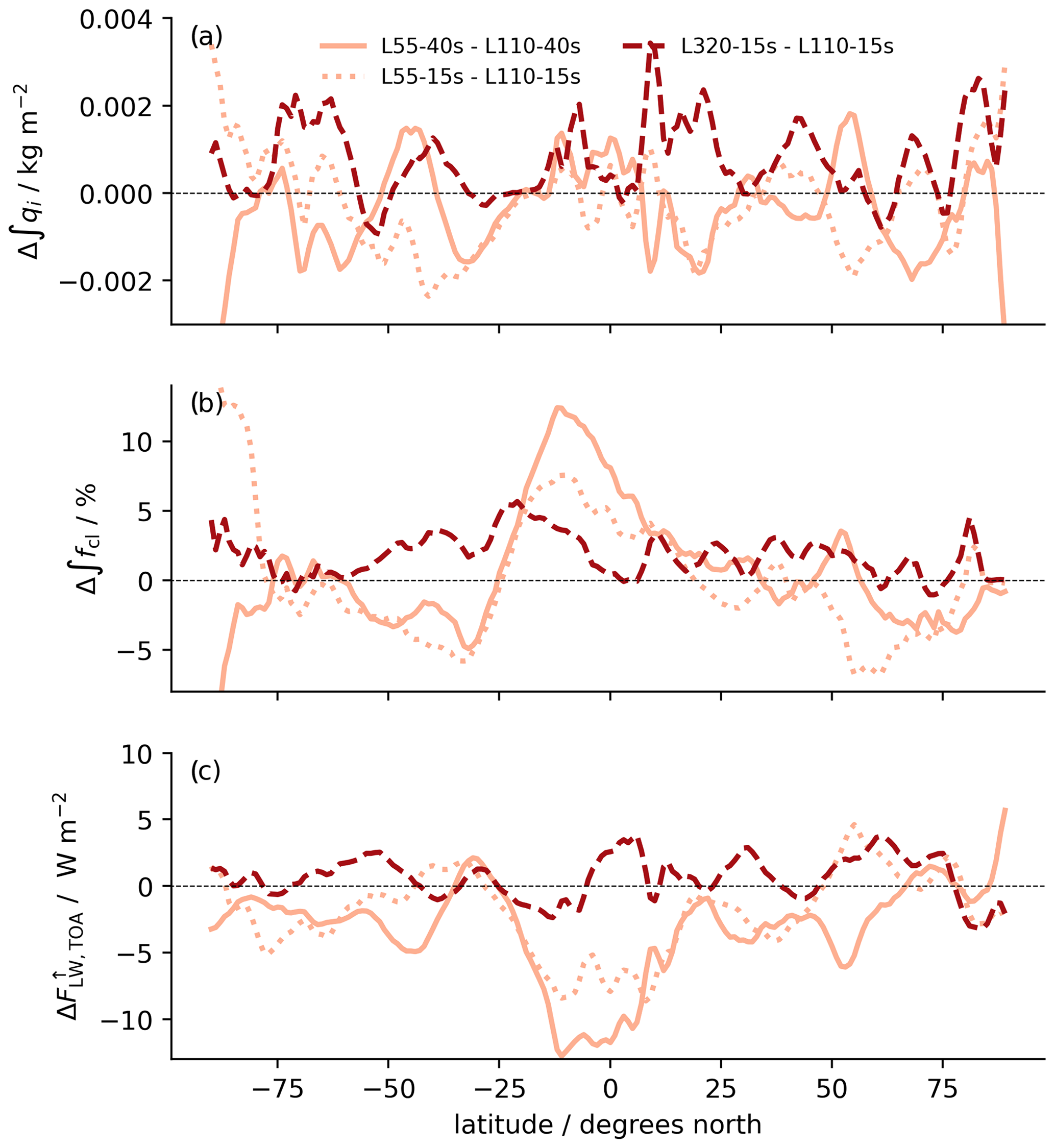
Figure 13 Differences in the zonally averaged atmospheric quantities between simulations, as indicated in the legend of panel (a). The quantities are (a) vertically integrated cloud ice (∫q_i), (b) total cloud fraction (∫f_cl), and (c) outgoing longwave radiation at the TOA ($F_{\mathrm{LW},\mathrm{TOA}}^{\downarrow }$). Solid lines mark differences in the practical vertical resolution changes (i.e., generally also including a time step change), the dashed line denotes a difference caused by a pure vertical resolution change, and the dotted line marks a difference caused by a pure time step change. All quantities are averaged over the last 40 d of the simulations.

The 4 % decrease in precipitation is consistent with the reduction in the latent heat flux and atmospheric radiative cooling, the latter of which is visible clearly in the reduction in the OLR. OLR is reduced by about 4.3 W m⁻² for the coarser vertical grid spacing in the case of L55-40s − L110-40s but only by about 2.6 W m⁻² in the case of L55-15s − L110-15s. Although the spreads are overlapping, we cannot exclude that the effect of the change in vertical grid spacing has a time step dependence. However, even the 2.6 W m⁻² effect is larger than any of the effects simulated for a refinement in the vertical or horizontal grids and merits further attention.

Figure 13 shows that the reduction in the OLR is dominated by a tropical signal, consistent with an increase in the cloud fraction that reaches a maximum of about 12 percentage points near 10^∘ S. Both signals are even larger than those of the maximum vertical grid refinement (L540-8s − L110-40s). By contrast, signals from a coarsening of the vertical grid spacing in cloud ice are relatively small, consistent with the global mean quantities. Due to the dominance of the tropical signals, it makes sense to discuss vertical profiles of quantities averaged over 30^∘ S–30^∘ N.

Similar to several global mean quantities (Fig. 2), experiment L55-40s also stands out in terms of the tropical profiles of, for instance, temperature and specific humidity, as the differences compared with the reference are larger than simulated in all experiments with refined vertical grid spacing. Temperature increases all over the troposphere with a maximum of about 1.3 K near 14 km, compared with a maximum decrease under a pure vertical grid refinement (L320-15s − L110-15s) of less than 0.5 K. Specific humidity increases by up to 50 % in the upper troposphere for a halving of the vertical resolution compared with a maximum decrease of about 10 % for quadrupling it. Relative humidity (Fig. 11) also increases much more strongly in the upper troposphere for the coarsening from L110-40s to L55-40s than it decreases for grid refinements. The strong moisture increase for the coarsening would reduce atmospheric radiative cooling and, hence, decelerate the overturning circulation. Lang et al. (2023) analyzed moisture differences in the tropical middle troposphere in our simulations L55-40s, L110-40s, L190-30s, and L110-2.5km as well as in further simulations with parameter changes. In general, the largest contribution to differences between different model configurations can be traced back to differences in the conditions that an air parcel experienced at the point of its last saturation. However, in the case of increased moisture due to the coarsening of the vertical grid spacing, about half of the increase cannot be explained by this last saturation paradigm. Lang et al. (2023) speculate that an increase in the numerical diffusion for coarser grids contributes to the moistening. Similar to our results, Ohno et al. (2019) also simulate the strongest increase in tropospheric humidity when switching to their coarsest vertical resolution with grid spacings in the upper troposphere of about 1 km.

While the refinement experiments cause increases in cloud ice at almost all altitudes, the signal of experiment L55-40s is characterized by an upward shift (Fig. 9) in the profile. The signal may be caused by the strongly increased moisture that shifts the maximum divergence of longwave radiative cooling and, thus, the divergence of vertical velocity in downwelling areas of the tropics and the convective anvils upward (e.g., Hartmann and Larson, 2002). In precipitation space (not shown), the signal of the grid coarsening is qualitatively consistent with, i.e., opposite to, the signal of the refinement shown in Fig. 12. However, with the relatively strong increase in the relative humidity, cloud ice also increases strongly in the dry regions. At altitudes near 13 km, this overcompensates for the reduction due to reduced upwelling in the moist regions.

The dipole in the upper tropospheric temperature anomaly in this simulation translates itself into an upward shift in the cold-point tropopause of about 1 km but hardly any change in the cold-point temperature.

As mentioned above, a remarkable feature of the L55-40s simulation is its strongly reduced OLR (by more than 4 W m⁻² globally and by more than 6 W m⁻² in the tropical average; Figs. 2d and 11f, respectively). The analysis of clear-sky fluxes (not shown) indicates that about half of this is a clear-sky effect related to the strongly increased tropospheric humidity (Fig. 10d). The other half can be explained by the increase in the ice cloud fraction (Fig. 11d). Analogous to the refinement experiment, where the ice cloud fraction is reduced everywhere in precipitation space, the coarsening leads to an increase everywhere (not shown). In the rainy regions, this increase occurs despite a decrease in the cloud ice amount. As discussed above, this apparent inconsistency in the moist regions can only be explained by less cloud ice being distributed to a larger number of grid cells.

Seiki et al. (2015) analyzed tropical cirrus in NICAM simulations at a 14 and 28 km horizontal grid spacing for different vertical grid spacings of about 100, 200, 400, and 1000 m in the upper tropical troposphere, i.e., comparable to our grids L320 to L55. In their simulations, differences in ice cloud quantities between the three finest grids are also much smaller than for the coarsest grid. Their and our results further agree on a comparable decrease in the OLR caused by the coarsest vertical grid spacing. However, the results differ with respect to other aspects. While our cloud fraction increases for the coarsest grid at basically all upper tropospheric altitudes, they report an increase only near the tropopause.

5 Comparing the effects of horizontal and vertical grid refinements

Figure 2a, d, and g show the differences in globally averaged water quantities and radiation fluxes of experiment L110-2.5km with respect to the reference experiment L110-40s, i.e., the effects of halving the horizontal grid spacing, in comparison with the differences in the experiments with refined vertical grids discussed above. The signs and magnitudes of the effects of the practical increase in the horizontal resolution presented here are generally in agreement with the effects reported and discussed by Hohenegger et al. (2020). Here, the purpose of showing horizontal resolution effects is to compare them with vertical resolution effects. To estimate the relative importance of a practical doubling of the horizontal resolution to a practical doubling of the vertical resolution, one may compare L110-2.5km − L110-40s with L190-30s − L110-40s. However, to judge the effects of comparable computing time investments in horizontal or vertical refinement, the comparison of L110-2.5km − L110-40s with L320-15s − L110-40s would be more appropriate. Independent of which vertical resolution experiment is chosen, the absolute effects of horizontal refinement are larger for precipitable water and shortwave radiation fluxes at both the TOA and the surface. The effects on longwave fluxes are of comparable magnitude. The absolute effect on cloud liquid water reaches a similar magnitude when the L320-15s experiment is used in the comparison, and the effect on cloud ice is larger in the vertical resolution experiments.

Robust (in the sense of the spread of the four individual subperiods not including zero) effects of horizontal and vertical refinements have different signs, in particular for cloud liquid water, shortwave fluxes, and the longwave surface flux. The signs of the longwave TOA flux differences are also opposite, although less robust. By contrast, the effect on cloud ice seems to point in the same direction, although it is less robust for horizontal refinement.

In the following, we will further discuss the relatively large effects on cloud condensate, in particular cloud liquid water, which is reduced by about 16 % in experiment L110-2.5km compared with L110-40s. As these experiments differ not only in the horizontal grid spacings of about 2.5 and 5 km but also in the time steps of 20 and 40 s, the time step effect could partly compensate for the horizontal resolution effect. If one assumes that the time step effect acts independently of spatial resolution changes, the pure effect of a doubling of the horizontal resolution could be 5 % larger. This suggests that necessary time step adaptations may reduce the effect of changing the horizontal grid but enhance the effect of changing the vertical grid.

The effects of practical vertical and horizontal resolution changes on net TOA shortwave radiation have opposite signs, which is consistent with the cloud liquid water changes. However, the shortwave radiative effect of horizontal refinement per unit change in the cloud water is larger than for vertical resolution.

Figure 6 shows that the reduction in the cloud liquid water with a practical increase in the horizontal resolution occurs fairly homogeneously all over the vertical profile in the tropics. As a shorter time step causes a qualitatively opposite effect, one can assume that the effect of a pure refinement in the horizontal grid spacing would cause an even larger but qualitatively similar reduction in cloud liquid water. The reduction in low clouds with higher horizontal resolution has been reported earlier in storm-resolving model simulations with ICON (Hohenegger et al., 2020) and NICAM (Noda et al., 2010). In contrast to the ICON simulations performed for this study and by Hohenegger et al. (2020), Noda et al. (2010) used a subgrid-scale shallow-cumulus parameterization. They show that increasing the ventilation of the boundary layer through parameter changes in this parameterization also decreases the low-cloud amount. This likely happens in ICON simulations due to a better resolution of shallow cumulus for finer horizontal grid spacing. Stevens et al. (2020) argue that a further refinement in the horizontal grid spacing to the hectometer scale could further improve these and other such cloud features.

Figure 7 shows that the changes in cloud liquid water in the South American stratocumulus region caused by a halving of horizontal grid spacing are of a similar magnitude to those caused by changes to the vertical grid spacing, despite much weaker effects on the structure of the boundary layer, as characterized by the profiles of temperature and humidity. We conjecture that the clouds are more directly affected by a change in horizontal grid spacing, which is still inadequately large for resolving shallow cumulus in this GSRM, but more indirectly by a change in the vertical grid spacing via a modified representation of the inversion.

In terms of the vertical distribution of cloud ice (Fig. 9), a refinement in the horizontal grid spacing has a comparable effect to refining the vertical grid but leads to an increase, even at very high altitudes up to about 17 km. Figure 10 shows that, similar to the vertical refinement effect, this is likely related to the increased convective activity, as indicated by the increased upwelling in moist regions.

6 Comparison to observations

In this section, we will present comparisons of selected simulated quantities with observations. The goal is not to provide a comprehensive evaluation of the simulations but rather to provide examples that illustrate the magnitude of grid refinement effects relative to overall model biases.

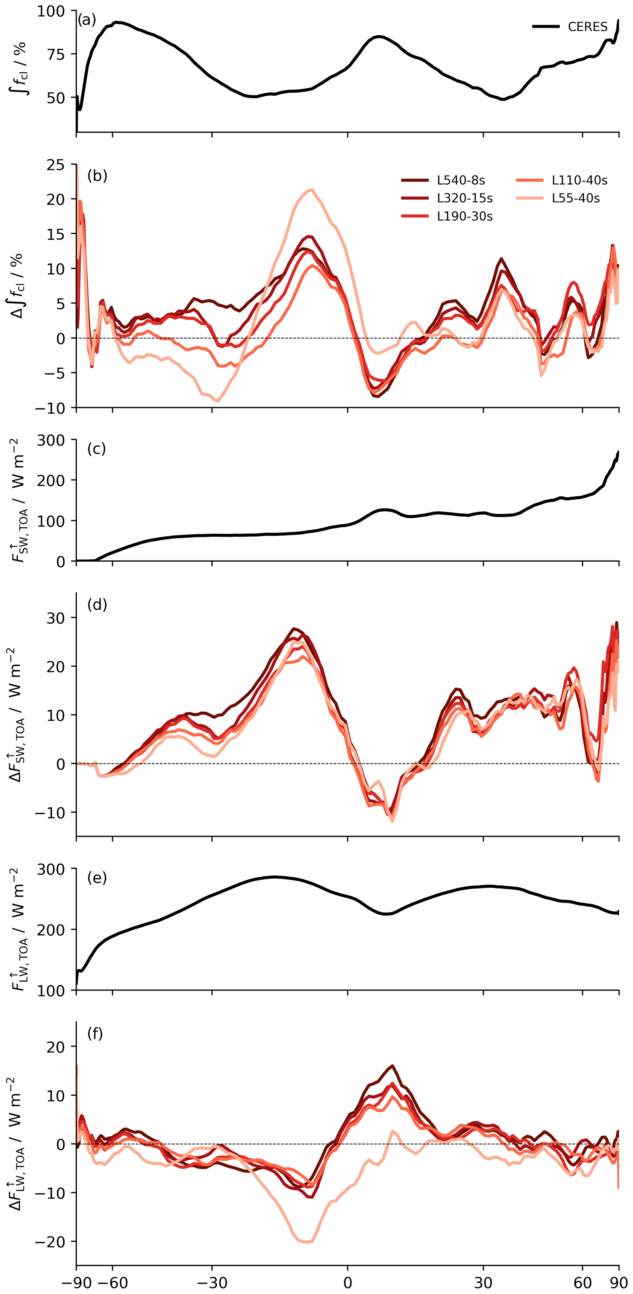
Figure 14 Zonally averaged (a) total cloud fraction (∫f_cl), (c) upward shortwave radiation at the TOA ($F_{\mathrm{SW},\mathrm{TOA}}^{\uparrow }$), and (e) upward longwave radiation at the TOA ($F_{\mathrm{LW},\mathrm{TOA}}^{\uparrow }$) from the CERES satellite observations averaged over July 2021. Panels (b), (d), and (f) show differences in the respective quantities between the simulations indicated in the legend and the satellite products.

Figure 14 shows the cloud fraction and the TOA upward shortwave and longwave fluxes from the Clouds and the Earth’s Radiant Energy System (CERES) project Energy Balanced and Filled (EBAF) satellite products (Kato et al., 2018; Loeb et al., 2018), edition 4.2, averaged over July 2021 in comparison with simulation results from the experiments for practical vertical resolution changes, i.e., the first five experiments listed in Table 1, averaged over the same time period. Again, the comparisons indicate that the L55-40s experiment is an outlier. All other experiments show relatively coherent biases, indicating that the dominant part of these biases is generally not caused by vertical truncation errors.

Over tropical and subtropical regions, the total cloud fraction is overestimated by the models, except for the ITCZ, slightly north of the Equator. The overestimation is likely related in part to the dependence of the cloud liquid water on the model resolution, as discussed in Sect. 5. Insufficient horizontal model resolution leads to too much low-level cloudiness. This effect is partially compensated for by a coarser vertical resolution. The underestimation directly at ITCZ latitudes may be related to the fact that the microphysics scheme of the ICON configuration used here represents frozen moisture in three categories, cloud ice, snow, and graupel, but only the first is considered in the radiation code and for the calculation of the cloud fraction. As one may expect, the biases in the outgoing shortwave radiation are generally correlated with those of the cloud fraction, while the biases in the outgoing longwave radiation are anticorrelated.

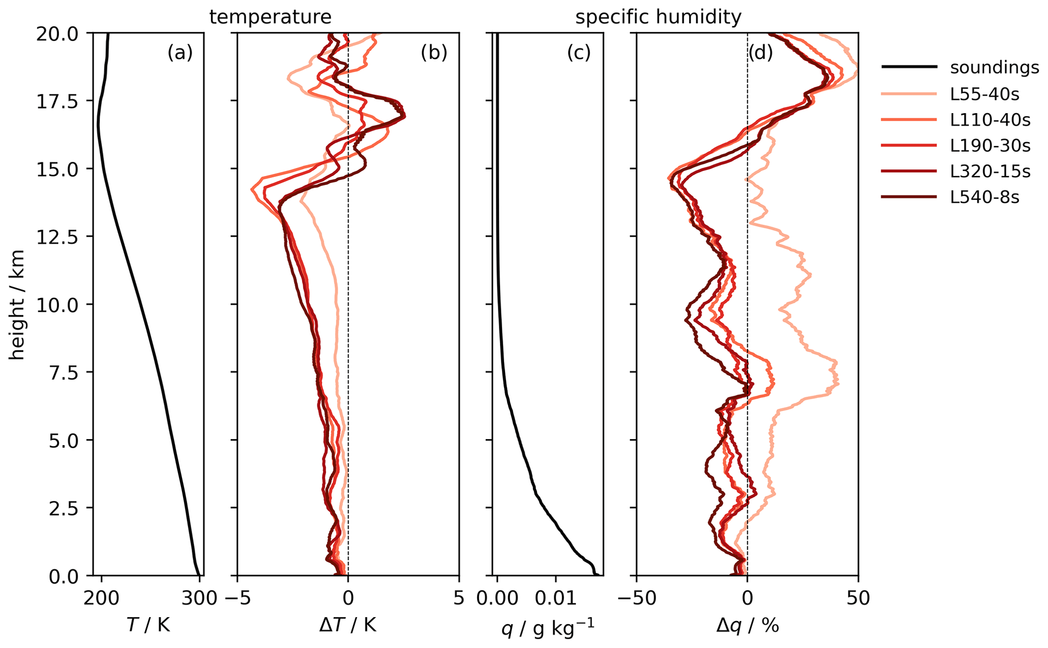
Figure 15 Mean vertical profiles of (a) temperature and (c) specific humidity from 257 radio soundings taken between 29 June and 6 August 2021 in the tropical Atlantic. Panels (b) and (d) show the differences in these observations compared with the mean simulated profiles for the simulations indicated in the legend and sampled at the time and location of the observations.

Figure 15 shows vertical profiles of temperature and specific humidity averaged from 257 radio soundings taken between 29 June and 6 August 2021 in the tropical Atlantic (Brandt et al., 2021; Schulz et al., 2022) in comparison with simulation results from the experiments for practical vertical resolution changes sampled at the time and location of the soundings. All simulations are colder at all tropospheric heights, and the biases increase with altitude. This increase in the biases is partly due to the cold biases in the lower troposphere and boundary layer, which are amplified in the upper troposphere when the lapse rate follows a moist adiabat. Another contribution to the biases comes from the lapse rate being more skewed to colder temperatures in the simulations. This is particularly evident for the L55-40s experiment, which shows very little bias in the lower troposphere.

It appears that all model configurations represent colder moist adiabats than observed. As discussed in Sect. 4, the coarsest grid (L55) produces higher tropospheric temperatures than those simulated with any of the other grids. Despite this, even the L55-40s simulation has a cold bias with respect to the radio soundings, although this is smaller than all other simulations. As mentioned earlier, L55-40s also has a moister troposphere than the other simulations. In comparison to the radiosondes, L55-40s simulates an overly high specific humidity at almost all tropospheric altitudes, while the other simulations have a dry bias, in particular in the upper troposphere. Relative humidity (not shown) is simulated better in all simulations except L55-40s.

Analogous to the zonal mean horizontal biases, the biases in the vertical profiles are similar for all experiments except L55-40s at most altitudes. An exception is the uppermost troposphere, where the cold bias is clearly reduced in L540-8s and L320-15s compared with coarser vertical grids. This hints at a better representation of the tropopause by finer grid spacing.

7 Summary and conclusions

The aim of this study is to quantify the effects of the choice of vertical grid spacing on the global climate simulated with the ICON-Sapphire GSRM at a 5 km horizontal grid spacing. We have analyzed 40 d simulated with boundary conditions for a period in the boreal summer of 2021 for five different vertical grids with between 55 and 540 vertical layers and maximum tropospheric grid spacings of between 800 and 50 m. The configuration with a 400 m maximum tropospheric spacing (L110) is close to the vertical grid typically used in ICON-Sapphire simulations (e.g., Hohenegger et al., 2023). While simulations with finer grids were generally run with shorter integration time steps to ensure numerical stability, additional simulations were run with three different vertical grids but identical time steps. This allows us to identify the contributions of the pure effects of changes in vertical grid spacing and of the integration time step to the effects of practical resolution changes, which generally result from a combination of both. Furthermore, we have run a simulation with halved horizontal grid spacing to compare the effects of vertical and horizontal grid choices.

A practical increase in the vertical resolution leads to changes in the global energy budget. The upward shortwave radiation at the TOA increases by about 2.5 W m⁻² when the number of vertical layers is increased from 110 to 540. The effect does not show any convergence for the vertical grids chosen here and can be attributed mostly to changes in low clouds. Globally averaged cloud liquid water increases by about 7 % for each practical doubling of the vertical resolution.

One can expect that the increase in cloud liquid water with finer vertical grid spacing should be particularly strong in stratocumulus regions, where the simulation of the inversion at the cloud top is likely to benefit from finer grid spacing. Such an effect is simulated in our experiments for stratocumulus in the Pacific off South America, but the signal is not robust over stratocumulus regions in general. Moreover, in the global average, more than half of the effects on cloud liquid water and shortwave radiation are related to the reduction in the integration time step needed to refine the grid spacing. Bogenschutz et al. (2021) also simulated an increase in the low-level cloudiness for finer vertical grid spacing, although in a GCM with larger horizontal grid spacing and convection parameterization. Contrary to our results, Bogenschutz et al. (2021) simulated a decrease in low-level cloudiness for a shorter time step. Wan et al. (2021) show that this sensitivity depends on the specifics of the numerical coupling of different processes in the model integration. To better understand and possibly reduce the time step effect in our model, a more detailed analysis of the numerical integration scheme would be required. However, our results confirm that the effects cannot necessarily be unambiguously attributed to the spatial discretization change when changes in model grid spacing require changes in the integration time step. On a more general note, this serves as a reminder that, while the shortest integration time step that avoids model crashes is often chosen for practical reasons, this choice can strongly affect the simulation results.

Refining the vertical grid spacing increases OLR in our experiments. However, this effect is generally much smaller than the effect on shortwave radiation. The OLR response can be traced back partly to changes in tropical cirrus clouds, of which, in the tropical average, the cloud fraction decreases with resolution while the total ice mass increases. Effects on the cloud ice concentration are different in moist tropical regions, where they are likely related to changes in convective activity, and in dry tropical regions, where they are consistent with changes in background conditions. In contrast to liquid clouds, the effects on tropical upper tropospheric ice clouds and OLR show a tendency to converge for the vertical resolutions tested here. A further difference is that these effects on cloud ice and OLR are dominated by the effect of the vertical grid spacing, while the influence of time step changes is negligible.

By far, the largest change in cloud ice is simulated for an increase of the maximum tropospheric vertical grid spacing from 400 m in the reference configuration L110-40s to 800 m in L55-40s. This reduces global OLR by more than 4 W m⁻². The coarsest resolution differs strongly from the other simulations with respect to several other quantities, such as tropical tropospheric temperature, specific, and relative humidity. A similar nonlinear response to vertical resolution changes has been simulated in the NICAM GSRM by Seiki et al. (2015) and in a NICAM RCE configuration by Ohno et al. (2019). Seiki et al. (2015) concluded from this that a vertical grid spacing of 400 m or less is required to accurately simulate tropical cirrus clouds. Our simulations support the conclusion that vertical grid spacing larger than 400 m would be inadequate for the simulation of tropical cirrus. More generally, the large effects simulated in ICON-Sapphire for a coarsening of the vertical grid spacing indicate a high price with respect to the computing time gains that could be obtained in such a configuration.

For most of the climate quantities studied here, doubling the vertical resolution beyond the L110 reference grid has smaller effects than doubling the horizontal resolution to a 2.5 km grid spacing. For example, cloud liquid water increases by about 7 % per practical doubling of the vertical resolution, whereas it decreases by about 16 % for the practical doubling of the horizontal resolution. Interestingly, the effects are of opposite sign. Effects of increases in the horizontal resolution on this quantity are, hence, counteracted by increases in vertical resolution. Such opposite sensitivities have also been obtained by Cheng et al. (2010) and Mellado et al. (2018) in LESs of inversion-topped stratocumulus clouds. Our results also confirm the importance of the aspect ratio of the vertical and horizontal resolution for the simulation of boundary layer clouds in GSRMs. More generally, our study emphasizes that the simulation of boundary layer clouds and associated effects in GSRMs is more susceptible to truncation errors than the simulation of many other quantities including, for instance, cirrus clouds.

Model biases with respect to observations are generally larger than differences between simulations with different vertical resolutions. This is shown by comparisons of simulation results with selected quantities from CERES satellite products and radio soundings. Simulations by Lang et al. (2023) show larger effects of changes in the parameterizations of microphysics and vertical turbulent diffusion on tropospheric temperature and relative humidity than those caused by the different grids of our L55-40s, L110-40s, and L190-30s simulations. These remaining parameterizations of GSRMs may be a promising target for reducing the simulation biases. This does not mean that truncation errors can be ignored. Future studies should evaluate the effects of the vertical resolution on the representation of specific climate features, as was done by authors such as Seiki et al. (2015) for tropical cirrus, where an improvement was shown for finer vertical grid spacing.

In the case of tropical vertical temperature profiles, the simulation with the largest a priori truncation error (L55-40s) is closer to the observations than any other of our model configurations. It is very likely that the truncation error compensates for other model deficiencies in this case. Similarly, the tropical cloud fraction outside of the ITCZ, and thus the reflected shortwave radiation, is overestimated most strongly in the simulation with the finest vertical grid (L540-8s). The increase in low-level cloudiness with finer vertical grid spacing simply enhances the overestimation related to an overly coarse horizontal grid spacing.

A central motivation for the investment in higher horizontal resolution in global atmospheric models is that the step to storm-resolving scales allows one to get rid of parameterizations, in particular for convection. Our analysis shows that, for the grids typically used in ICON and other GSRMs today, the effect of halving the horizontal grid spacing is larger than the effect of halving the vertical grid spacing for most climate quantities. However, the effects are of the same order of magnitude. As doubling the vertical resolution is computationally cheaper than doubling the horizontal resolution, we conclude that further computing time investments in vertical refinement may affect the truncation errors of GSRMs similarly to comparable investments in horizontal refinement. Our study clearly shows that coarser vertical grid spacing than that used in our 110-layer reference grid is inadequate. However, specific climate features such as boundary layer clouds show no convergence, even for a grid with a maximum tropospheric layer thickness of 50 m, which is much finer than what is currently used in most GSRMs.