Development of the tangent linear and adjoint models of the global online chemical transport model MPAS-CO₂ v7.3

We describe the development of the tangent linear (TL) and adjoint models of the Model for Prediction Across Scales (MPAS)-CO₂ transport model, which is a global online chemical transport model developed upon the non-hydrostatic Model for Prediction Across Scales – Atmosphere (MPAS-A). The primary goal is to make the model system a valuable research tool for investigating atmospheric carbon transport and inverse modeling. First, we develop the TL code, encompassing all CO₂ transport processes within the MPAS-CO₂ forward model. Then, we construct the adjoint model using a combined strategy involving re-calculation and storage of the essential meteorological variables needed for CO₂ transport. This strategy allows the adjoint model to undertake a long-period integration with moderate memory demands. To ensure accuracy, the TL and adjoint models undergo vigorous verifications through a series of standard tests. The adjoint model, through backward-in-time integration, calculates the sensitivity of atmospheric CO₂ observations to surface CO₂ fluxes and the initial atmospheric CO₂ mixing ratio. To demonstrate the utility of the newly developed adjoint model, we conduct simulations for two types of atmospheric CO₂ observations, namely the tower-based in situ CO₂ mixing ratio and satellite-derived column-averaged CO₂ mixing ratio ($X_{{\mathrm{CO}}_{\mathrm{2}}}$). A comparison between the sensitivity to surface flux calculated by the MPAS-CO₂ adjoint model with its counterpart from CarbonTracker–Lagrange (CT-L) reveals a spatial agreement but notable magnitude differences. These differences, particularly evident for $X_{{\mathrm{CO}}_{\mathrm{2}}}$, might be attributed to the two model systems' differences in the simulation configuration, spatial resolution, and treatment of vertical mixing processes. Moreover, this comparison highlights the substantial loss of information in the atmospheric CO₂ observations due to CT-L's spatial domain limitation. Furthermore, the adjoint sensitivity analysis demonstrates that the sensitivities to both surface flux and initial CO₂ conditions spread out throughout the entire Northern Hemisphere within a month. MPAS-CO₂ forward, TL, and adjoint models stand out for their calculation efficiency and variable-resolution capability, making them competitive in computational cost. In conclusion, the successful development of the MPAS-CO₂ TL and adjoint models, and their integration into the MPAS-CO₂ system, establish the possibility of using MPAS's unique features in atmospheric CO₂ transport sensitivity studies and in inverse modeling with advanced methods such as variational data assimilation.

1 Introduction

Estimating CO₂ fluxes through inverse modeling, using atmospheric chemical transport models and atmospheric CO₂ measurements, is an important approach for understanding the global carbon budget. Beyond providing seasonal flux estimates that are useful for understanding the magnitude and phase of photosynthesis and respiration, it provides annual mean flux estimates that shed light on the key processes driving the response to climate change. When these annual mean CO₂ estimates are adjusted to account for lateral fluxes (e.g., due to rivers or the transport of crops and wood products), it gives an independent means of validating carbon stock change estimates from the terrestrial biogeochemical models and inventories (Byrne et al., 2023). However, atmospheric transport models, which play a key role in inverse modeling, remain a significant source of uncertainty at both regional and global scales (Schuh et al., 2019, 2022; Hurtt et al., 2022).

Two classes of chemical transport models – online and offline – are commonly used for simulating atmospheric CO₂ transport. Offline models, such as TM5 (Krol et al., 2005; Meirink et al., 2006), PCTM (Kawa et al., 2004; Baker et al., 2006), and GEOS-Chem (Kopacz et al., 2009), solve the tracer continuity equation using winds and vertical mixing fields computed from an independent run of a meteorological model or from a meteorological analysis. Online models, such as WRF-Chem (Grell et al., 2011), OLAM (Walko and Avissar, 2008; Schuh et al., 2021), and MPAS-CO₂ (Skamarock et al., 2012; Zheng et al., 2021), integrate chemistry, transport, and meteorology simultaneously. Although offline models typically have lower computational costs, the separation of chemistry and transport from meteorology leads to a loss of information regarding atmospheric processes occurring at timescales shorter than the meteorological model output frequency (Grell et al., 2005). In comparison, online models, owing to their simultaneous integration of meteorology and chemistry, have the potential to improve transport accuracy, particularly for vertical transport of chemistry. Recent advances in computer power and parallelization have greatly reduced the computational cost of online transport models, making them increasingly more accessible and practical for atmospheric CO₂ research.

A number of studies have demonstrated that transport model accuracy can be improved by increasing the model's horizontal resolution (Feng et al., 2016; Agusti-Panareda et al., 2019). Because global high-resolution CO₂ transport simulations are computationally demanding, limited-area models (regional models) are often used instead (Pillai et al., 2012; Lauvaux et al., 2012; Zheng et al., 2018). However, regional models introduce the lateral boundary condition, posing challenges for CO₂ inverse modeling (Zheng et al., 2019; Rayner et al., 2019). As a global online chemical transport model, the Model for Prediction Across Scales (MPAS)-CO2 (Zheng et al., 2021) avoids the lateral boundary condition problem. Like OLAM (Schuh et al., 2021), MPAS-CO₂ uses a global variable-resolution mesh to facilitate local grid refinement for high-resolution simulations in specific regions without incurring prohibitively high computational costs and avoiding the disadvantages of lateral boundary conditions.

The primary objective of this study is to develop the tangent linear (TL) and adjoint (AD) models associated with the global online transport model MPAS-CO₂ (Zheng et al., 2021). Adjoint model techniques have been widely used in both meteorological and atmospheric greenhouse gas research (Errico, 1997; Courtier et al., 1994; Giering et al., 2006; Meirink et al., 2008; Henze et al., 2007; Tian and Zou, 2021) and play critical roles in variational data assimilation and sensitivity analyses (Baker et al., 2006; Zheng et al., 2018; Tian and Zou, 2020).

The subsequent sections of this paper provide an overview of the MPAS-CO₂ forward model developed in Zheng et al. (2021) (Sect. 2) and the development and verification of the TL and AD models based on the forward model (Sects. 3 and 4). The utility of the newly developed AD model is demonstrated with adjoint sensitivity analyses in Sect. 5. Finally, a summary and conclusions are given in Sect. 6.

2 MPAS-CO₂ forward model

Zheng et al. (2021) documented the development of MPAS-CO₂, verifying its mass conservation and assessing its accuracy. Hereafter, we refer to MPAS-CO₂ as the forward model, whose TL and AD model counterparts we develop in the present paper. A brief description of the forward model is provided here; see Zheng et al. (2021) for comprehensive details. The forward model characterizes CO₂ transport through the continuity equation, as follows:

$$\begin{array}{}\text{(1)}& {\displaystyle \frac{\partial \left(\stackrel{\mathrm{̃}}{\mathit{\rho }}{q}_{{\mathrm{CO}}_{\mathrm{2}}}\right)}{\partial t}}=-{\left(\mathrm{\nabla }\cdot \stackrel{\mathrm{̃}}{\mathit{\rho }}{q}_{{\mathrm{CO}}_{\mathrm{2}}}\mathit{V}\right)}_{\mathit{\zeta }}+F_{\text{bl}}+F_{\text{cu}},\end{array}$$

where $q_{{\mathrm{CO}}_{\mathrm{2}}}$ is CO₂ dry-air mixing ratio, $\stackrel{\mathrm{̃}}{\mathit{\rho }}={\mathit{\rho }}_{\mathrm{d}}/(\partial \mathit{\zeta }/\partial z)$, ρ_d is dry-air density, ζ is the vertical coordinate, z is geometric height, t is time, and $\mathit{V}=(u,v,w)$ is the velocity vector (u, v, and w are the zonal, meridional, and vertical wind components, respectively). The meteorological variables, such as wind velocity and dry-air density, are updated simultaneously with CO₂ by the model's dynamical core and physics parameterizations. The left-hand side (LHS) of Eq. (1) is the total CO₂ time tendency ($\partial \left(\stackrel{\mathrm{̃}}{\mathit{\rho }}{q}_{{\mathrm{CO}}_{\mathrm{2}}}\right)/\partial t$). The first term on the right-hand side (RHS) represents the contributions to CO₂ time tendency from the advection. The second (F_bl) and third (F_cu) terms of RHS represent the contribution from the vertical mixing by the planetary boundary layer (PBL) and cumulus convective transport parameterizations, respectively. Advection of CO₂ in MPAS-CO₂ is handled in the model's dynamical core and can be expressed as Eq. (2), where the first two terms on the RHS represent the horizontal advection, and the third term represents the vertical advection:

$$\begin{array}{}\text{(2)}& \begin{array}{rl}{\left(\mathrm{\nabla }\cdot \stackrel{\mathrm{̃}}{\mathit{\rho }}{q}_{{\mathrm{CO}}_{\mathrm{2}}}\mathit{V}\right)}_{\mathit{\zeta }}=& {\left[{\displaystyle \frac{\partial \left(\stackrel{\mathrm{̃}}{\mathit{\rho }}u{q}_{{\mathrm{CO}}_{\mathrm{2}}}\right)}{\partial x}}+{\displaystyle \frac{\partial \left(\stackrel{\mathrm{̃}}{\mathit{\rho }}v{q}_{{\mathrm{CO}}_{\mathrm{2}}}\right)}{\partial y}}\right]}_{\mathit{\zeta }}\\ & +{\displaystyle \frac{\partial \left(\stackrel{\mathrm{̃}}{\mathit{\rho }}w{q}_{{\mathrm{CO}}_{\mathrm{2}}}\right)}{\partial \mathit{\zeta }}}.\end{array}\end{array}$$

CO₂ vertical mixing by the PBL parameterization is implemented based on the YSU scheme (Hong et al., 2006) and can be expressed as

$$\begin{array}{}\text{(3)}& {\left[{\displaystyle \frac{\partial q_{{\mathrm{CO}}_{\mathrm{2}}}}{\partial t}}\right]}_{\text{bl}}={\displaystyle \frac{\partial }{\partial z}}\left[K_{\mathrm{h}}\left({\displaystyle \frac{\partial q_{{\mathrm{CO}}_{\mathrm{2}}}}{\partial z}}\right)-\stackrel{\mathrm{‾}}{{\left(w^{\prime }{q}_{{\mathrm{CO}}_{\mathrm{2}}}^{\prime }\right)}_{\mathrm{h}}}{\left({\displaystyle \frac{z}{h}}\right)}^{\mathrm{3}}\right],\end{array}$$

where z is the vertical distance to the surface, h is the boundary layer top height, and K_h is the vertical eddy diffusivity. The second term on the RHS in the square bracket of Eq. (3) represents the contribution from CO₂ entrainment flux at the inversion layer. The term $[\partial q_{{\mathrm{CO}}_{\mathrm{2}}}/\partial t{]}_{\text{bl}}$ from Eq. (3) is coupled with dry-air density $\stackrel{\mathrm{̃}}{\mathit{\rho }}$ to form the term F_bl of Eq. (1).

Convective transport of CO₂ is implemented based on the Kain–Fritsch convection scheme (Kain, 2004), and it can be expressed as Eq. (4):

$$\begin{array}{}\text{(4)}& \begin{array}{rl}{\left[{\displaystyle \frac{\partial q_{{\mathrm{CO}}_{\mathrm{2}}}}{\partial t}}\right]}_{\text{cu}}=& {\displaystyle \frac{(M_{\mathrm{u}}+M_{\mathrm{d}})}{\mathit{\rho }A}}{\displaystyle \frac{\partial q_{{\mathrm{CO}}_{\mathrm{2}}}}{\partial z}}+{\displaystyle \frac{M_{\text{ud}}}{M}}\left(q_{{\mathrm{CO}}_{\mathrm{2}}}^{\mathrm{u}}-q_{{\mathrm{CO}}_{\mathrm{2}}}\right)\\ & +{\displaystyle \frac{M_{\text{dd}}}{M}}\left(q_{{\mathrm{CO}}_{\mathrm{2}}}^{\mathrm{d}}-q_{{\mathrm{CO}}_{\mathrm{2}}}\right),\end{array}\end{array}$$

where $q_{{\mathrm{CO}}_{\mathrm{2}}}$, $q_{{\mathrm{CO}}_{\mathrm{2}}}^{\mathrm{u}}$, and $q_{{\mathrm{CO}}_{\mathrm{2}}}^{\mathrm{d}}$ are the CO₂ mixing ratio in the environment, updraft, and downdraft, respectively; M_u and M_d are the updraft and downdraft mass, respectively; ρ is the environment air density; A is the horizontal area of a cell; M=ρAδz is the mass of environmental air in a grid box; and M_ud and M_dd are the detrainment from the updraft and downdraft, respectively. The term $[\partial q_{{\mathrm{CO}}_{\mathrm{2}}}/\partial t{]}_{\text{cu}}$ of Eq. (4) is coupled with dry-air density $\stackrel{\mathrm{̃}}{\mathit{\rho }}$ to form the term F_cu of Eq. (1).

3 Development of the MPAS-CO₂ TL model

3.1 TL model development

The CO₂ advective transport process described in Eq. (2) is implemented by two different numerical schemes in the forward model: (1) a monotonic scheme with hyperviscosity (β) set to 0.25; and (2) a non-monotonic scheme with β=1.0 (Skamarock et al., 2012). The monotonicity in the first scheme is achieved by applying a flux limiter in the last step of the third-order Runge–Kutta solver (Wang et al., 2009; Skamarock and Gassmann, 2011). While the second scheme is linear in CO₂, the first scheme is nonlinear due to the application of the flux limiter. Because both the YSU PBL and Kain–Fritsch convection schemes are linear in CO₂, using the linear advective scheme makes the forward model a linear model in CO₂. In this paper, we develop the TL and adjoint models based on the linear version of the MPAS-CO₂ forward model, which can be symbolically expressed as

$$\begin{array}{}\text{(5)}& x_{\mathrm{t}}=\mathcal{M}(x_{\mathrm{0}},e),\end{array}$$

where x₀ and x_t are the CO₂ dry-air mixing ratio at the initial and forecast time (t), respectively. ℳ( ) represents the MPAS-CO₂ forward model, and e represents a time series of CO₂ fluxes between times 0 and t. While both x₀ and x_t are 3-dimensional in space, e is 2-dimensional in space, indicating that CO₂ flux is applied only to the model's surface cells. Equation (5) indicates that CO₂ mixing ratio at a forecast time (x_t) is determined by the CO₂ mixing ratio at an initial time (x₀) and the CO₂ flux (e) through the forward model.

The TL and adjoint models are designed to calculate the sensitivity of x_t with respect to x₀ and e. This is achieved by introducing the TL and adjoint variables of their counterparts in the forward model (Giles and Pierce, 2000). While the introduction of the TL and adjoint variables for the initial CO₂ mixing ratio (x₀) is straightforward, it is a bit more complex for the CO₂ fluxes (e). This complexity arises from the fact that CO₂ flux, at each surface cell of the model, varies with time throughout the model's entire simulation period. Depending on the underlying biosphere model and emission inventory used, CO₂ flux varies at a certain temporal frequency, ranging from hourly to monthly. Although it is possible to introduce TL and adjoint variables for CO₂ flux at the flux's temporal frequency, it is neither practical nor necessary to do so. Instead, a common approach is to introduce flux scaling factors (Henze et al., 2007; Zheng et al., 2018) as follows:

$$\begin{array}{}\text{(6)}& e=S\left(\mathit{k}\right)\stackrel{\mathrm{̃}}{e},\end{array}$$

where $\stackrel{\mathrm{̃}}{e}$ are time-variant CO₂ fluxes, typically from a process model or inventory, and S(k) is a generic scaling function. Equation (6) means that at each surface cell, the magnitude of the CO₂ flux ($\stackrel{\mathrm{̃}}{e}$) is adjusted using a flux scaling factor before it is used to modify the cell's CO₂ mixing ratio. We implemented Eq. (6) in the forward model in a way that allows the flexibility of choosing the temporal frequency of the flux scaling factor. For instance, for a 24 h forward model simulation forced by 3 h CO₂ flux, one can choose to have eight scaling factors at each surface cell (one for each of the eight 3 h segments) or just one scaling factor for the entire time period. All the MPAS-CO₂ model runs used in the remainder of this paper are conducted using a single scaling factor for each surface cell that is repeated for each flux time step in the entire simulation period. In this case, the scaling function S(k) in Eq. (6) is a function of a scaling vector k that has the same dimension as the model's surface mesh. The introduction of the flux scaling factors turns CO₂ flux from active variables to parameters, and the impacts of their variation on CO₂ mixing ratio are calculated through their corresponding scaling factors k. Accordingly, the MPAS-CO₂ forward model can be symbolically expressed as

$$\begin{array}{}\text{(7)}& x_{\mathrm{t}}=\mathcal{M}(x_{\mathrm{0}},\mathit{k}).\end{array}$$

Equation (7) shows that for a given set of CO₂ flux ($\stackrel{\mathrm{̃}}{e}$), the forecast time CO₂ mixing ratio (x_t) is a function of the initial time CO₂ mixing ratio (x₀) and the flux scaling factor (k).

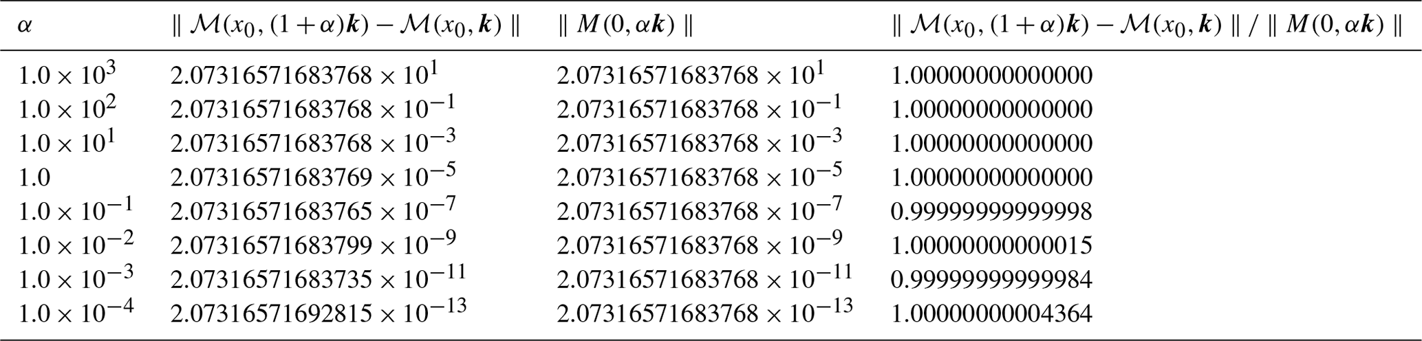
Table 1 Results of the correctness check for the newly developed MPAS-CO₂ tangent linear model. The results are from 1 month integration (from 1 October 2018 at 00:00 UTC to 1 November 2018 at 00:00 UTC) of the forward and tangent linear models, using the 120–480 km global variable-resolution mesh (Fig. 1). The terms in the table refer to Eq. (9).

The TL counterpart of the MPAS-CO₂ forward model represented by Eq. (7) can be symbolically expressed as the first derivative of the forward model:

$$\begin{array}{}\text{(8)}& \mathrm{\Delta }{x}_{\mathrm{t}}=M(\mathrm{\Delta }{x}_{\mathrm{0}},\mathrm{\Delta }\mathit{k}),\end{array}$$

where M( ) represents the MPAS-CO₂ TL model, Δx₀ and Δx_t are the TL variable of CO₂ mixing ratio at the initial and forecast time, respectively, and Δk is the TL variable of the flux scaling factor k. In essence, Eq. (8) shows that the TL model computes the perturbation in the forecast time CO₂ mixing ratio (Δx_t), given the perturbation in the flux scaling factor (Δk) and/or perturbation in the initial time CO₂ mixing ratio (Δx₀).

Based on the source code of the forward model, we developed the TL code by differentiating each process relevant to CO₂ flux and transport, including advection, vertical mixing by the YSU PBL scheme, convective transport by the Kain–Fritsch scheme, and the CO₂ emission driver that implements Eq. (6). Automatic differentiation tools, such as Tapenade (Hascoet and Pascual, 2013) and Tangent and Adjoint Model Compiler (Giering and Kaminski, 1998), can be used to assist TL and adjoint code generation. However, the code these tools generate typically contains redundancies and is difficult to read, particularly for the adjoint code. To optimize the computation efficiency and facilitate future code upgrading, we manually developed the TL and adjoint code for MPAS-CO₂ with some minor assistance from Tapenade.

3.2 TL model validation

After the TL model is completed, a thorough examination of its correctness was undertaken. As indicated in Eq. (8), the TL model can calculate the sensitivity of x_t with respect to both x₀ and k. The calculation of the sensitivity of x_t with respect to x₀ involves the TL code of all the CO₂ transport processes, including advection, PBL, and convective transport. In comparison, the calculation of the sensitivity of x_t with respect to the flux scaling factor k involves the TL code of the CO₂ emission driver in addition to the TL code of all the CO₂ transport processes. Because the calculation of sensitivity to k includes the TL code of all the processes in the TL model and because both the transport processes and emission driver are linear, the correctness of the entire MPAS-CO₂ TL model can be verified by checking whether the following equation is satisfied (Errico, 1997; Tian and Zou, 2020):

$$\begin{array}{}\text{(9)}& \mathrm{\Phi }\left(\mathit{\alpha }\right)={\displaystyle \frac{\parallel \mathcal{M}({\mathbf{x}}_{\mathbf{0}},(\mathrm{1}+\mathit{\alpha }\left)\mathit{k}\right)-\mathcal{M}({\mathbf{x}}_{\mathbf{0}},\mathit{k})\parallel }{\parallel M(\mathrm{0},\mathit{\alpha }\mathit{k})\parallel }}=\mathrm{1},\end{array}$$

where M() is the TL model, ℳ() is the forward model, and α is a scalar. The second item in the numerator of Eq. (9), ℳ(x₀,k), is a forward model run. The first item in the numerator, $\mathcal{M}({\mathbf{x}}_{\mathbf{0}},(\mathrm{1}+\mathit{\alpha }\left)\mathit{k}\right)$, is an identical forward model run, except that its flux scaling factor at each surface cell is adjusted by multiplying 1+α. In the denominator, M(0,αk) is a TL model run with its perturbation in the initial time CO₂ mixing ratio set to zero (Δx₀=0) and perturbation in flux scaling factor Δk=αk, which is the difference in the flux scaling factors between the two forward model runs.

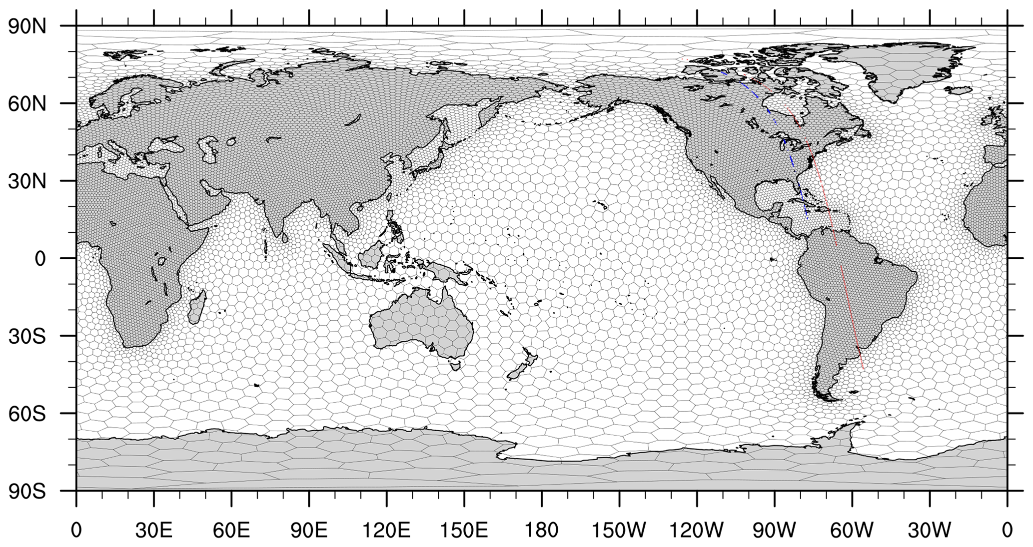
Figure 1 A MPAS-CO₂ global variable resolution mesh ranging from ∼ 120 km over most of land regions to ∼ 480 km over oceans. Also shown in the figures are the ground tracks of two Orbiting Carbon Observatory-2 orbits, which are used for the adjoint sensitivity studies described in Sect. 5. The blue-colored ground track crosses North America from the Caribbean Sea northward between 18:31 UTC and 18:48 UTC on 30 June 2016. The red-colored ground track crosses from South America to North America between 17:36 UTC and 18:13 UTC on 23 August 2016.

If the TL model is correctly coded with regard to the forward model, Eq. (9) should be satisfied to the extent of machine accuracy until α is too small, so that the result is affected by rounding-off errors and drifts away from unity. To verify using Eq. (9), we ran a series of simulations using the forward model and newly developed tangent linear model with the scale factor α ranging from 1.0 × 10³ to 1.0 × 10⁻⁴ (Table 1). All of the simulations start on 1 October 2018 at 00:00 UTC, run for 1 month, and end on 1 November 2018 at 00:00 UTC. The meteorological initial condition is from the ERA5 reanalysis (Hoffmann et al., 2019), and the CO₂ initial condition (x₀) is from CarbonTracker (Jacobson et al., 2020) v2022 (CT2022) posterior CO₂ mole fraction at this time. The 3 h CO₂ fluxes for the biogenic, fire, fossil fuel, and oceanic components from the CT2022 posterior are applied throughout the 1-month simulation period for each model run. Flux scaling factors of k=1 were used in all our simulations here, with 1 being a vector the same length as k, with ones in every element. The model simulations are conducted using the global variable-resolution (VR) mesh shown in Fig. 1. This VR mesh has a total of 15 898 cells, which range from 120 km over most of the land regions to 480 km over oceans. Table 1 shows that the magnitudes of both the numerator and the denominator in Eq. (9) decrease as α decreases. Moreover, the table also shows that the ratio remains close to unity until α decreases to 1.0 × 10⁻¹, beyond which rounding-off errors lead to a deviation from unity. These results confirm that the MPAS-CO₂ TL model has been correctly developed with regard to the forward model. In the next section, we proceed to develop the MPAS-CO₂ adjoint model.

4 Development of the MPAS-CO₂ adjoint model

4.1 Adjoint model development

An adjoint model is an essential component of a variational data assimilation system and is very useful for adjoint sensitivity analysis (Tian and Zou, 2021; Zheng et al., 2018; Bosman and Krol, 2023). Symbolically, the MPAS-CO₂ adjoint model can be expressed as

$$\begin{array}{}\text{(10)}& \left(\mathrm{\Delta }{\widehat{x}}_{\mathrm{0}},\mathrm{\Delta }\widehat{\mathit{k}}\right)=M^{\mathrm{T}}\left(\mathrm{\Delta }{\widehat{x}}_t\right),\end{array}$$

where M^T() is the MPAS-CO₂ adjoint model, $\mathrm{\Delta }\widehat{\mathit{k}}$ is the adjoint variable of the flux scaling factor, and $\mathrm{\Delta }{\widehat{x}}_{\mathrm{0}}$ and $\mathrm{\Delta }{\widehat{x}}_t$ are the adjoint variables of CO₂ mixing ratio at the initial and forecast time, respectively. Equation (10) shows that starting with $\mathrm{\Delta }{\widehat{x}}_t$ at the forecast time, the MPAS-CO₂ adjoint model runs backward in time to the initial time, while ingesting CO₂ observations along the way, resulting in the adjoint variable of CO₂ mixing ratio at the initial time ($\mathrm{\Delta }{\widehat{x}}_{\mathrm{0}}$) and the adjoint variable of the flux scaling factor ($\mathrm{\Delta }\widehat{\mathit{k}}$).

Similar to its TL model counterpart, the development of the MPAS-CO₂ adjoint model was carried out through manual implementation to avoid redundancy and optimize computational efficiency. The calculation of the CO₂ transport needs access to the meteorological fields at each time step. Since the forward and TL model both run forward in time, this access is straightforward. However, because the adjoint model runs backward in time, accessing the meteorological fields is more challenging. One approach to this problem is saving meteorological fields in memory during the adjoint model's forward sweep, enabling accessing during the subsequent backward sweep (Guerrette and Henze, 2015; Zheng et al., 2018). However, since the MPAS-CO₂ adjoint model is intended for long simulations, this approach becomes impractical due to the excessive memory it demands. As an alternative strategy, we adopt an approach that combines both recalculation and storage of the meteorological fields. This strategy effectively divides a long simulation into segments, and the forward and backward sweeps are carried out sequentially for each segment, requiring internal memory only large enough to accommodate one segment's worth of meteorological fields. This internal manipulation is handled seamlessly by the adjoint model, enabling it to run as long as needed without overburdening memory resources. Another strategy we adopted for developing the adjoint code is to have the forward sweep, save some immediate variables that are needed by the subsequent backward sweep so that they do not need to be recalculated. For instance, the values of some variables related to mass fluxes in the Kain–Fritsch convection scheme Kain (2004) are saved by the forward sweep in the memory to speed up the subsequent backward sweep execution. This strategy not only increases the adjoint model efficiency but also simplifies some of its code development.

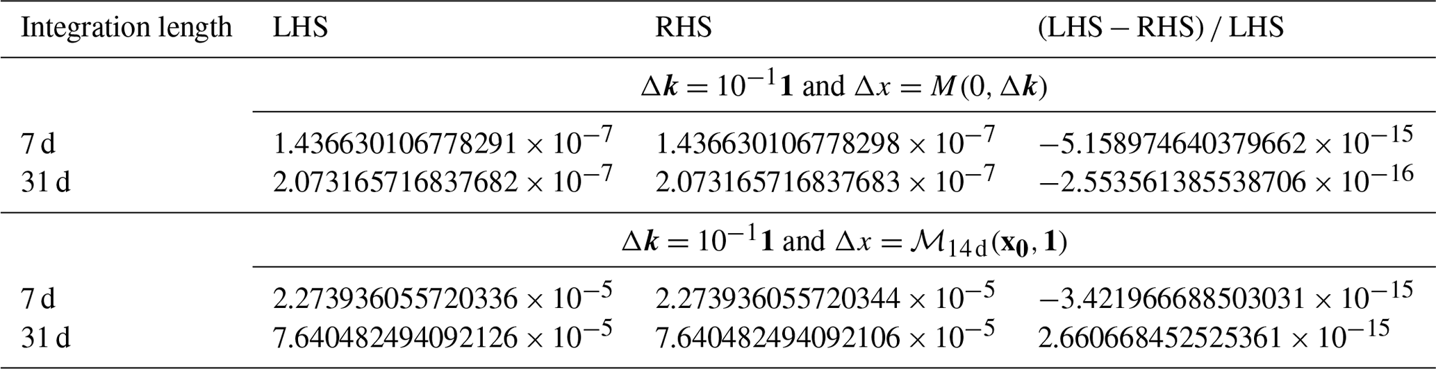
Table 2 Results of the correctness check for the newly developed adjoint model of MPAS-CO₂. All simulations are of the 120–480 km variable-resolution mesh (Fig. 1). The LHS and RHS in the table refer to Eq. (11).

4.2 Adjoint model validation

The correctness of the newly developed MPAS-CO₂ adjoint model can be verified using the following equation (Tian and Zou, 2020):

$$\begin{array}{}\text{(11)}& \langle \mathrm{\Delta }x,M(\mathrm{0},\mathrm{\Delta }\mathit{k})\rangle =\langle M^{\mathrm{T}}\left(\mathrm{\Delta }x\right),\mathrm{\Delta }\mathit{k}\rangle ,\end{array}$$

where 〈 〉 represents the inner product operator, Δx is a perturbation of CO₂ mixing ratio, and Δk is a perturbation of CO₂ flux scaling factor. If the adjoint model is correctly coded with respect to the TL model, then Eq. (11) should be satisfied for any choice of Δx and Δk. M(0,Δk) on the LHS of the equation is the perturbation in forecast CO₂ mixing ratio resulting from a TL model run whose perturbation in initial CO₂ mixing ratio is set to zero and perturbation to flux scaling factor is set to Δk. The first item of the RHS, M^T(Δx), represents the adjoint variable of flux scaling factor, which is an output from the adjoint model integration from the forecast time backward to the initial time. The TL and adjoint model runs on the two sides of Eq. (11) have the same simulation time period, but the latter runs backward in time.

We conducted two sets of experiments using the TL and adjoint models following Eq. (11) to verify the correctness of the newly developed adjoint model. In the first set of experiments, we set $\mathrm{\Delta }\mathit{k}={\mathrm{10}}^{-\mathrm{1}}\mathbf{1}$, and $\mathrm{\Delta }x=M(\mathrm{0},\mathrm{\Delta }\mathit{k})$. The experiments were carried out in two steps. First, the TL model was integrated 7 d from the initial time (1 October 2018 at 00:00 UTC) to the end time (8 October 2018 at 00:00 UTC), with $\mathrm{\Delta }\mathit{k}={\mathrm{10}}^{-\mathrm{1}}\mathbf{1}$, resulting in M(0,Δk) which is the perturbation in forecast time CO₂ mixing ratio. Second, the adjoint model is initialized on 8 October 2018 at 00:00 UTC, with its adjoint variable for CO₂ mixing ratio set to M(0,Δk). The adjoint model is then integrated backward in time for 7 d to 1 October 2018 at 00:00 UTC, resulting in M^T(Δx). The LHS and RHS of Eq. (11) are then calculated using the above results (Table 2). The table shows that the agreement between the LHS and RHS of Eq. (11) is about −5.16 × 10⁻¹⁵. We note that this value is not exactly zero due to the machine rounding errors. This experiment is repeated with the same configuration, but the simulation length is increased to 31 d, ending on 1 November 2018 at 00:00 UTC. As expected, the magnitude of both the LHS and RHS increased, and they agreed to about −2.55 × 10⁻¹⁶. In the second set of experiments, $\mathrm{\Delta }\mathit{k}={\mathrm{10}}^{-\mathrm{1}}\mathbf{1}$ (same as the first set of experiments) but $\mathrm{\Delta }x={\mathcal{M}}_{\mathrm{14}\mathrm{d}}(x_{\mathrm{0}},\mathit{k})$, which is the CO₂ mixing ratio at the end of 14 d forward model run (1 October 2018 at 00:00 UTC to 15 October 2018 at 00:00 UTC). We note that this forward model run uses x₀ from CT2022 posterior CO₂ mole fraction, and k=1; however, Eq. (11) should satisfy for any configuration and simulation period of the forward model. The resulting LHS and RHS of Eq. (11) from the second set of experiments are about 2 orders of magnitude larger than their counterpart of the first experiments. This is caused by the much larger Δx of the second set of experiments. The LHS and RHS agree to about −3.42 × 10⁻¹⁵ for the 7 d simulation and about 2.66 × 10⁻¹⁵ for the 31 d simulation (Table 2).

The results shown in Table 2 obtained from the experiments based on Eq. (11) confirm that the MPAS-CO₂ adjoint model has been correctly developed with regard to the TL model. As the TL model has already been confirmed correct with respect to the forward model, it follows that both TL and adjoint models are correct with respect to the forward model of MPAS-CO₂. This validation ensures the reliability and integrity of the entire MPAS-CO₂ model system, since the forward model has already been validated in Zheng et al. (2021). It allows MPAS-CO₂ to be used as the basis of a variational assimilation system for carbon flux estimation and as a platform for conducting sensitivity analyses in atmospheric carbon research.

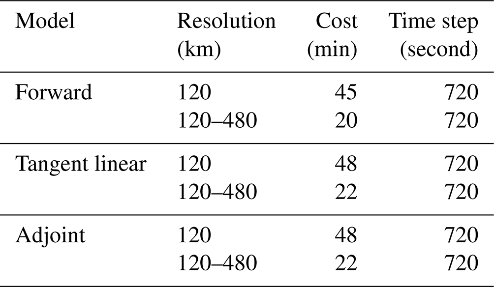
Table 3 presents the computational cost of model simulations using the MPAS-CO₂ system. Using the global 120–480 km VR mesh (Fig. 1; 15 898 cells), the 1-month forward model simulation completes in 20 min when using 128 processors. Both the TL and adjoint model simulations using the same configuration take approximately 10 % longer than the forward model. This extra computation time for the TL/adjoint model is incurred by the execution of the TL/adjoint code of the CO₂ transport processes. Furthermore, we conducted another set of 1-month simulations using the models on a global quasi-uniform resolution (UR) mesh of about 120 km, consisting of a total of 40 962 cells. Table 3 demonstrates that the simulations with the VR mesh reduce the computational cost by over 50 % for all three models, primarily due to its substantially smaller number of cells. This reduction in computation cost, while preserving the high resolution over areas of interest, should prove advantageous when the models are applied in variational assimilation problems, which typically require many iterations of forward and adjoint model runs.

Table 3 The computational costs for a 30 d simulation of MPAS-CO₂ at ∼ 120 km quasi-uniform resolution and at a variable resolution ranging from ∼ 120 to ∼ 480 km. Computational costs are shown for the forward, tangent linear, and adjoint models. All simulations are conducted using 128 AMD Epyc 7H12 2.595 GHz processors running in parallel.

5 Adjoint sensitivity analysis

5.1 Comparison with CT-L footprints

In addition to forming a key component of variational assimilation systems (Baker et al., 2006; Zheng et al., 2018; Tian and Zou, 2021), adjoint models are powerful tools for sensitivity analysis (Errico and Vukicevic, 1992; Errico, 1997; Zou et al., 1997; Tian and Zou, 2020). Studies focused on carbon flux estimation are often interested in exploring the sensitivity of atmospheric CO₂ measurements to surface CO₂ fluxes. This sensitivity is commonly referred to as observation influence functions or footprints (Cui et al., 2022). The computation of observation footprints using forward models requires a large number of model runs, making it impractical, except for optimizing state vector elements at coarse horizontal resolutions. In contrast, adjoint models can calculate observation footprints much more efficiently. For point measurements, such as those from tower data, Lagrangian dispersion models offer an efficient alternative for obtaining footprints (Lin et al., 2003; Stohl et al., 2005). For an example of this, see the publicly available CO₂ observation footprints from CarbonTracker–Lagrange (CT-L) (Hu et al., 2019), which are generated using the Lagrangian particle dispersion model STILT (Lin et al., 2003), driven by meteorology generated by the Weather Research and Forecast (WRF) model (Skamarock et al., 2008). This approach involves releasing a certain number of particles from the observation location/height and tracing their backward transport in time. Note that CT-L is a regional modeling system that only provides observation footprints within the latitude range 10^∘–80^∘ N and longitude 0–180^∘ W for up to 10 d backward in time.

In this section, we perform sensitivity analyses using the MPAS-CO₂ adjoint model, which employs backward-in-time integration to calculate two quantities: (1) the sensitivity of atmospheric CO₂ to the model's initial CO₂ mixing ratio and (2) the sensitivity to the surface flux scaling factor. When a spatially uniform time-invariant surface flux of a unity value is used, and S(k)=k in Eq. (6), the sensitivity to the surface flux scaling factor calculated by the MPAS-CO₂ adjoint model is the observation footprint. To compare with CT-L footprints, all MPAS-CO₂ adjoint model simulations conducted in this section use a time-invariant CO₂ surface fluxes of 1.0 µmol (m² s)⁻¹ for all surface cells, including both land and ocean cells. Because S(k)=k is used, Eq. (6) takes the form of $e=\mathit{k}\stackrel{\mathrm{̃}}{e}$. The units of the CO₂ flux ($\mathrm{\mu }\mathrm{mol}{\mathrm{m}}^{-\mathrm{2}}{\mathrm{s}}^{-\mathrm{1}}$) and the multiplicative nature of the flux scaling factor k determine the units of the adjoint variable $\mathrm{\Delta }\widehat{\mathit{k}}$ (which represents observation footprints) to be in $\mathrm{ppm}(\mathrm{\mu }\mathrm{mol}{\mathrm{m}}^{-\mathrm{2}}{\mathrm{s}}^{-\mathrm{1}}{)}^{-\mathrm{1}}$. Meteorological initial conditions for MPAS-CO2 model simulations conducted in this section are from the ERA5 reanalysis (Hoffmann et al., 2019). Footprints calculated by the MPAS-CO₂ adjoint model are of the 120–480 km variable resolution grid, while the CT-L footprints are of 1^∘ × 1^∘.

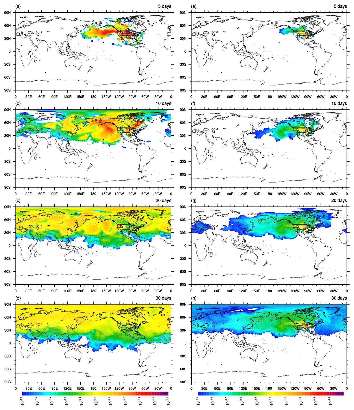
Figure 2 Sensitivity of CO₂ mixing ratio at the WKT tower at 00:00 UTC on 31 March 2018 to the initial CO₂ mixing ratio (a–d; units in ppm ppm⁻¹) and the surface flux scaling factor (e–h; units in $\mathrm{ppm}(\mathrm{\mu }\mathrm{mol}{\mathrm{m}}^{-\mathrm{2}}{\mathrm{s}}^{-\mathrm{1}}{)}^{-\mathrm{1}}$. The four rows from top to bottom show the sensitivities at 5, 10, 20, and 30 d before the observation. The sensitivities to the initial CO₂ mixing ratio (a–d) are plotted as the column average. The WKT tower (31.3149^∘ N, 97.3269^∘ W) measurements used here are taken at 457 m above the ground level and labeled by the red color cross in the figures of the left column (a–d).

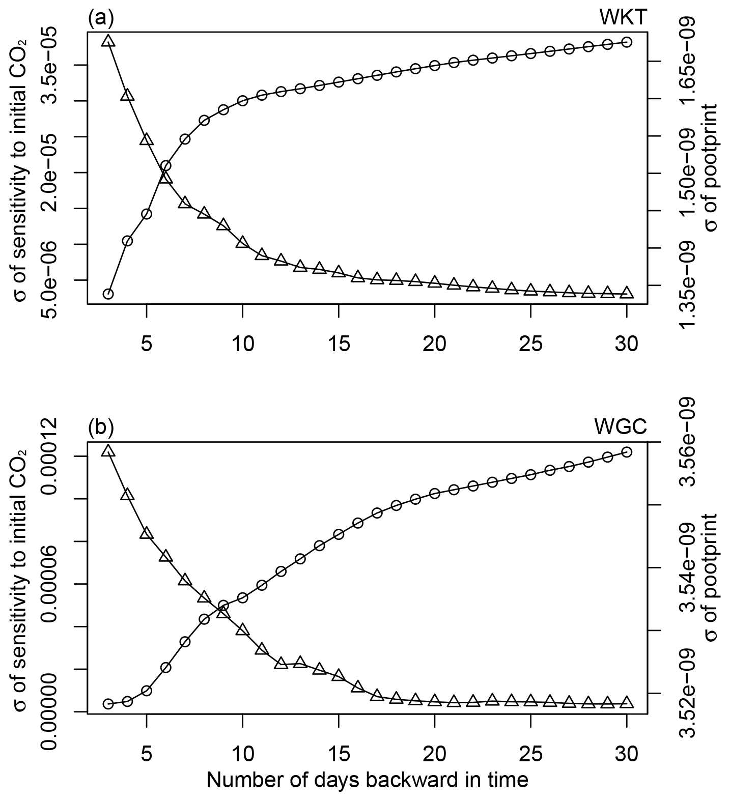
Figure 3 The variation over time in the standard deviation (σ) of two quantities: the sensitivity to the initial CO₂ mixing ratio and the sensitivity to the flux scaling factor (footprint). The standard deviations were calculated from MPAS-CO₂ adjoint model simulations starting on 31 March 2018 at 00:00 UTC, running 30 d backward in time, and ending on 1 March 2018 at 00:00 UTC. Panel (a) is for the WKT tower (457 $\mathrm{m}\mathrm{a}.\mathrm{g}.\mathrm{l}.$) while panel (b) is for the WGC tower (483 $\mathrm{m}\mathrm{a}.\mathrm{g}.\mathrm{l}.$). In each figure, the triangles represent the standard deviation of sensitivity to the CO₂ mixing ratio field (units in ppm ppm⁻¹), and the circles represent the standard deviation of footprint (units in $\mathrm{ppm}(\mathrm{\mu }\mathrm{mol}{\mathrm{m}}^{-\mathrm{2}}{\mathrm{s}}^{-\mathrm{1}}{)}^{-\mathrm{1}}$).

First, we conduct MPAS-CO₂ adjoint model simulations for in situ CO₂ observations at two towers in the United States, namely WKT, located at Moody, Texas (31.31^∘ N, 97.33^∘ W), and WGC, located at Walnut Grove, California (38.26^∘ N, 121.49^∘ W). For each tower, the adjoint model is initialized at 00:00 UTC on 31 March 2018. We add an adjoint forcing of 1 ppm CO₂ at that time to the model grid cell closest to the tower location and the intake height (457 m at WKT and 483 m at WGC). The forcing is turned off for subsequent time steps, and the adjoint model is run backward in time for 30 d, ending at 00:00 UTC on 1 March 2018. The resulting sensitivity of CO₂ at the WKT tower to the model's CO₂ mixing ratio, which is 3-dimensional, is shown as a column average in the left column of Fig. 2. The right column of Fig. 2 shows the observation footprint (sensitivity to the surface flux scaling factor) at the corresponding times. The figure panels show that the sensitivity to the initial CO₂ is highest and concentrated closest to the tower site at the time closest to the measurement, i.e., 5 d. With the increasing length of the backward-in-time integration, the sensitivity spreads over a larger area, and its magnitude decreases. After 30 d, the sensitivity to the initial condition has propagated across most of the Northern Hemisphere. Figure 2 also indicates that the spatial variation in the sensitivity magnitude decreases with time. To examine this, we calculated the standard deviation (σ) of sensitivity for each day of the 30 d (Fig. 3). The triangles in Fig. 3 show that the magnitude of the standard deviation of the sensitivity to the initial CO₂ mixing ratio decreases rapidly with the increasing length of the adjoint model simulation for both towers. On the other hand, the sensitivity to the surface flux scaling factor (footprint) exhibits a different pattern from the sensitivity to the initial CO₂ mixing ratio. As shown in Fig. 2, the footprint spreads spatially but the near-field to the tower maintains a much higher magnitude than the far-fields. By the end of 30 d, the footprint of the WKT tower covers almost the entire Northern Hemisphere, with the area north and northwest of the tower within the contiguous United States exhibiting a much higher magnitude than the more distant area. The circles in Fig. 3 indicate that the standard deviation of the footprint increases with time, but the rate of increase diminishes substantially after about 10 to 15 d. The finding suggests that extending the adjoint model integration further backward in time will still result in changes to the footprint but with a much-reduced change rate.

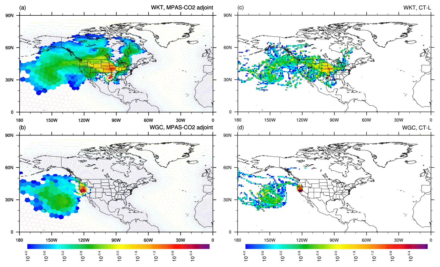
Figure 4 The 10 d backward in time CO₂ measurement footprint (units in $\mathrm{ppm}(\mathrm{\mu }\mathrm{mol}{\mathrm{m}}^{-\mathrm{2}}{\mathrm{s}}^{-\mathrm{1}}{)}^{-\mathrm{1}}$) given by two tall towers, namely WKT and WGC. The figures in the top row are the footprint of the WKT tower calculated using the MPAS-CO₂ adjoint model (a) and CT-L (c). The figures in the bottom row are the footprint of the WGC tower calculated by the MPAS-CO₂ adjoint model (b) and CT-L (d). The location of the towers is marked by the black crosses in the figures in the right column (c, d).

For comparison, in Fig. 4, we plot the MPAS-CO₂ adjoint model-calculated 10 d footprints in the CT-L geographic domain. The figure reveals that the MPAS-CO₂ adjoint model-calculated WKT tower footprint spans most of the western and northwestern United States, with the highest sensitivity in Texas, Missouri, Iowa, Kansas, and Nebraska. Additionally, the footprint extends to a substantial area over the northeastern Pacific Ocean. The spatial pattern of the CT-L calculated footprint (Fig. 4c) is similar to that from the MPAS-CO₂ adjoint model, but it is visibly less continuous. Figure 4 also shows that the MPAS-CO2 adjoint model-calculated footprint for the WGC tower covers northern California, Oregon, west Nevada, and a portion of the northeastern Pacific Ocean. The CT-L-calculated footprint exhibits a similar spatial pattern and magnitude. Overall, both the MPAS-CO₂ adjoint model and CT-L provide valuable information on the sensitivity of atmospheric CO₂ measurements to the surface flux; there are similar spatial patterns, although with some differences due to resolution and the Lagrangian/Eulerian framework difference.

In the second set of experiments, we compare CT-L and MPAS-CO₂ adjoint model footprints for a swath of Orbiting Carbon Observatory-2 (OCO-2) $X_{{\mathrm{CO}}_{\mathrm{2}}}$ measurements. The ground track of the OCO-2 orbit used in the experiments is indicated by the blue line in Fig. 1. This orbit crosses North America from the Caribbean Sea to Canada's Northwest Territories in a northward direction between 18:31 UTC and 18:48 UTC on 30 June 2016. Since OCO-2 $X_{{\mathrm{CO}}_{\mathrm{2}}}$ represents the column average of atmospheric CO₂, CT-L calculates $X_{{\mathrm{CO}}_{\mathrm{2}}}$ footprints at 14 discrete height levels, ranging from 50 to 14 000 m above the ground. For each height level, footprints are computed by placing a number of particles at that specific height. To ensure consistency with the CT-L approach, the MPAS-CO₂ adjoint model is configured to apply the adjoint forcing at the corresponding vertical levels within the model. This is done by interpolating the CT-L's 14 height levels to MPAS-CO2 model's 55 vertical levels. This configuration allows for a direct comparison between the footprints calculated by the MPAS-CO₂ adjoint model and the CT-L footprints.

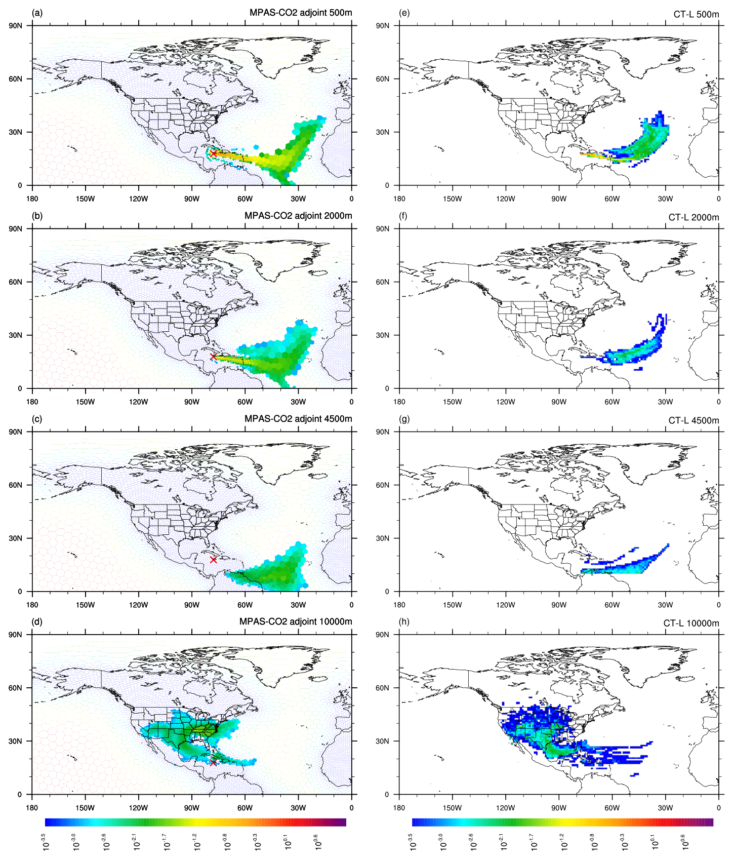
Figure 5 Comparison of footprints calculated by MPAS-CO₂ adjoint model and CT-L of an OCO-2 sounding (17.82^∘ N, 77.88^∘ W) (red crosses; a–d) along the ground track shown in Fig. 1 (blue color). The footprints are calculated at four different heights: 500, 2000, 4500, and 10 000 m, and 10 d backward in time.

Figure 5 shows the footprints of a point located south of Jamaica in the Caribbean Sea (17.82^∘ N, 77.88^∘ W) at four different height levels: 500, 2000, 4500, and 10 000 m. The top three rows of Fig. 5 show that both the MPAS-CO₂ adjoint model and CT-L footprints largely extend eastward over the Atlantic Ocean, indicating transport from the surface due to the influence of the easterly trade winds. Additionally, the MPAS-CO₂ adjoint model-calculated footprint includes a branch that crosses the Equator and extends southeastward to the Southern Hemisphere between 30 and 40^∘ W longitude. This feature is not shown in the CT-L footprint due to its limited area domain. The bottom row of Fig. 5 shows that the footprints of 10 000 m calculated by both the MPAS-CO₂ adjoint and CT-L feature a primarily counterclockwise extension, covering the Gulf of Mexico and Texas. Moreover, there is a second segment extending westward from Texas toward the west coast. Upon closer examination, we observe that the CT-L-calculated footprint has a lower magnitude than the MPAS-CO₂ adjoint model at the 500, 2000, and 4500 m height levels but not at the 10 000 m height level. The distinct patterns in both systems' footprints at different height levels indicate significant differences in horizontal and vertical transport patterns.

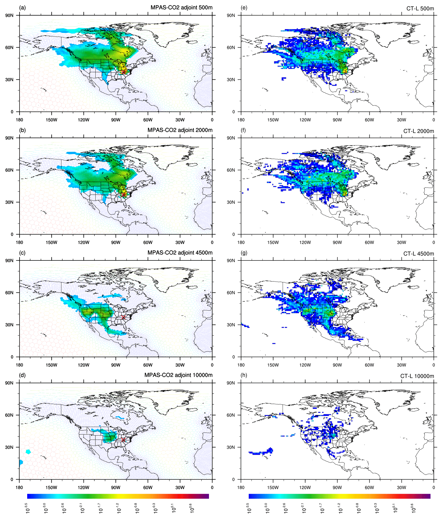
Figure 6 Same as Fig. 5, except for a different OCO-2 sounding location (36.8^∘ N, 82.9^∘ W).

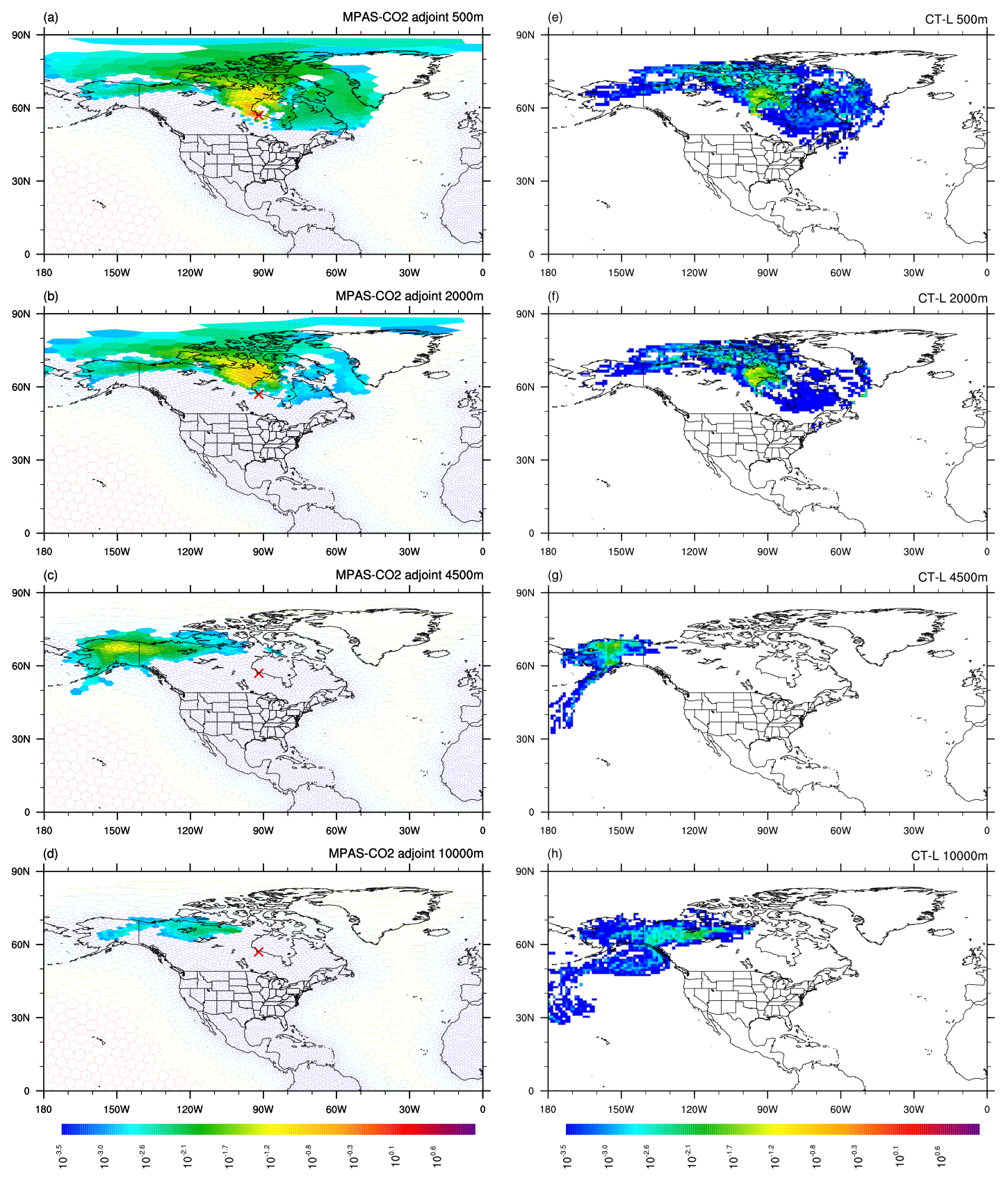
Figure 7 Same as Fig. 5, except for a different OCO-2 sounding location (56.96^∘ N, 91.89^∘ W).

Figure 6 shows the corresponding footprints for an OCO-2 $X_{{\mathrm{CO}}_{\mathrm{2}}}$ sounding location in eastern Kentucky (36.8^∘ N, 82.9^∘ W) for the same four height levels as shown in Fig. 5. The figure shows that the footprints of 500 and 2000 m extend predominantly northward, covering the Great Lakes region and part of the Canadian Shield. In comparison, the footprint for 4500 m is mostly directed to the west. Another notable difference is that the highest-magnitude portion of the 500 and 2000 m footprints are in close proximity to the sounding location, while the 4500 m footprint is not in proximity at all. These differences among the height levels are evident in both the MPAS-CO₂ adjoint model and CT-L calculated footprints. Figure 7 shows the footprints of an OCO-2 sounding location on the southwest coast of Hudson Bay, Canada (56.96^∘ N, 91.89^∘ W), for the four height levels. Both the MPAS-CO₂ adjoint and CT-L footprints for 500 and 2000 m are largely either close to or north of the sounding location, indicating that surface fluxes from these regions have a significant influence on the atmospheric CO₂ at the two height levels. In comparison, the footprint of 4500 m is located more than 2000 km northwestward, mostly covering Alaska; the particles move that far in a horizontal manner in the time it takes them to advect and mix 4500 m in the vertical. These findings emphasize the significant impact of vertical mixing on the spatial distribution of footprint at different altitudes, highlighting the unique patterns of horizontal and vertical transport in each case.

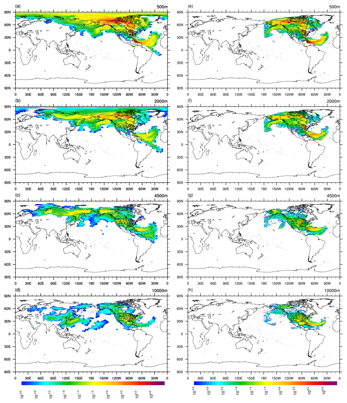
Figure 8 The footprint of the OCO-2 ground track shown in Fig. 1 (with blue color) calculated by the MPAS-CO₂ adjoint model (a–d) and by CT-L (e–h). The footprints are calculated by placing the adjoint forcing (for the MPAS-CO2 adjoint model) or releasing particles (for CT-L) at four different height levels above the ground: 500, 2000, 4500, and 10 000 m. The footprints are computed for 10 d backward in time.

In additional MPAS-CO₂ adjoint model runs, we quantitatively compare the footprints of the entire OCO-2 track at each of the 14 height levels with the CT-L footprints. This comparison is conducted by performing a single MPAS-CO₂ adjoint model run for each height level to calculate the footprint at the end of the 10 d backward-in-time integration. We then compare these resulting footprints with their CT-L counterparts. Figure 8 shows the comparison at four height levels of 500, 2000, 4500, and 10 000 m above the surface. At each height level, the value in the figure represents the average of the footprints of all the cells that are part of the OCO-2 track. The figure reveals that the footprints calculated by the two systems have similar spatial patterns within the limited-area domain of CT-L. However, it is important to note that a substantial portion of the footprints extends beyond the CT-L domain. For instance, the footprints of 2000 and 4500 m levels have significant coverage over Siberia in Russia, while the footprint of the 10 000 m level extends from the eastern Pacific Ocean to northeastern and western China, both of which are outside the CT-L model domain.

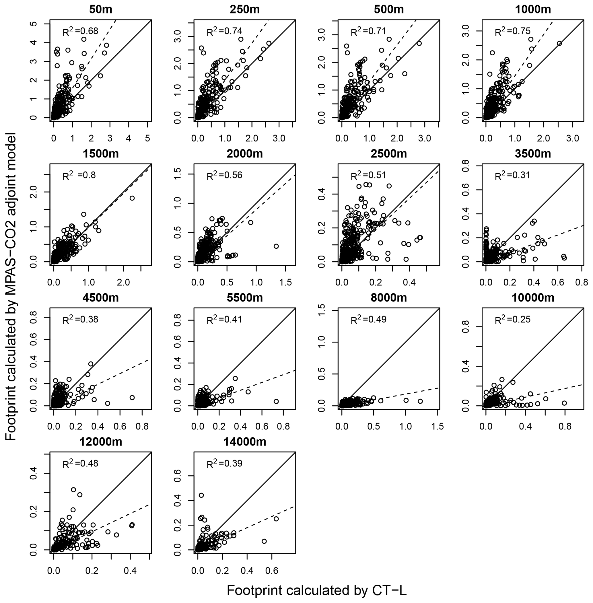
Figure 9 Comparison of the OCO-2 ground track footprints from the MPAS-CO₂ adjoint model and CT-L after 10 d backward-in-time integration. For each of the 14 height levels, the values of the footprints (units in $\mathrm{ppm}(\mathrm{\mu }\mathrm{mol}{\mathrm{m}}^{-\mathrm{2}}{\mathrm{s}}^{-\mathrm{1}}{)}^{-\mathrm{1}}$) are extracted as the average value of 2^∘ × 3^∘ boxes within the range of the CT-L spatial domain (10–80^∘ N, 0–180^∘ W). The solid line in each subfigure is the 1:1 line, and the dashed line is a linear fit with zero intercept. The correlation coefficient R² of the linear fit is also labeled in each subfigure.

In order to compare the footprints from the two systems quantitatively, we aggregated the footprints onto a 2^∘ × 3^∘ (lat × long) grid within the area covered by the CT-L model domain for each of the 14 height levels. Figure 9 shows the comparison for each of the 14. In the figure, the CT-L calculated footprints are on the x axis, and MPAS-CO₂ adjoint model calculated footprints are on the y axis. The solid line in each subfigure of Fig. 9 is the 1:1 line, and the dashed line is a linear fit without intercept. The correlation coefficient R² is labeled in each subfigure. The figure demonstrates that the agreement between the two systems is better for footprints at lower heights, particularly between 250 and 1500 m, with R² all greater than 0.7. Footprints from the two systems agree to a much lesser degree at between 3500 and 14 000 m, where R² is less than 0.5 in all cases. The linear fit lines (dashed lines) show that the MPAS-CO₂ adjoint model calculated footprints are of greater magnitude in general than their CT-L counterparts at heights ranging from 50 to 1000 m. Between 1500 and 2500 m, the two sets of footprints are of similar magnitude on average, and at 3500 m and above, the CT-L footprints are of larger magnitude in general.

These differences in magnitude between the two systems could be attributed to various factors, including differences in model configurations, spatial resolution, and treatment of vertical mixing processes. Previous studies have shown that Lagrangian models, such as CT-L, can sometimes have different vertical mixing behavior compared to Eulerian models, especially at high altitudes (Karion et al., 2019).

5.2 Influence of vertical distribution of OCO-2 soundings on footprints

In a final experiment, we use the MPAS-CO₂ adjoint model to examine the impact of different vertical distributions on footprint calculation. Two adjoint model simulations were conducted for the OCO-2 orbit that crosses South America and North America between 17:36 UTC and 18:13 UTC on 23 August 2016 (the red color track in Fig. 1). Both simulations have the same adjoint forcing of 1 ppm $X_{{\mathrm{CO}}_{\mathrm{2}}}$ added to each MPAS-CO₂ model cell along the orbital track at 18:00 UTC on 23 August 2016 and run backward in time for 30 d. The difference between the two simulations lies in the vertical distributions of the adjoint forcing. For the first simulation, we adopt profile 1, which is obtained by combining the $X_{{\mathrm{CO}}_{\mathrm{2}}}$ averaging kernel and pressure weight function (O'Dell et al., 2018). In contrast, profile 2 prioritizes $X_{{\mathrm{CO}}_{\mathrm{2}}}$ information in the lower part of the troposphere (Fig. 10). The 20 pressure levels in the figure are interpolated to the MPAS-CO₂ model's 55 vertical levels for the adjoint forcing placement. This experiment aims to highlight how these differences in vertical distribution impact the footprint calculation, leading to variations in flux estimation using variational assimilation. The results of this experiment will provide valuable insights to the importance of selecting appropriate vertical distribution when using the adjoint model for CO₂ flux estimation.

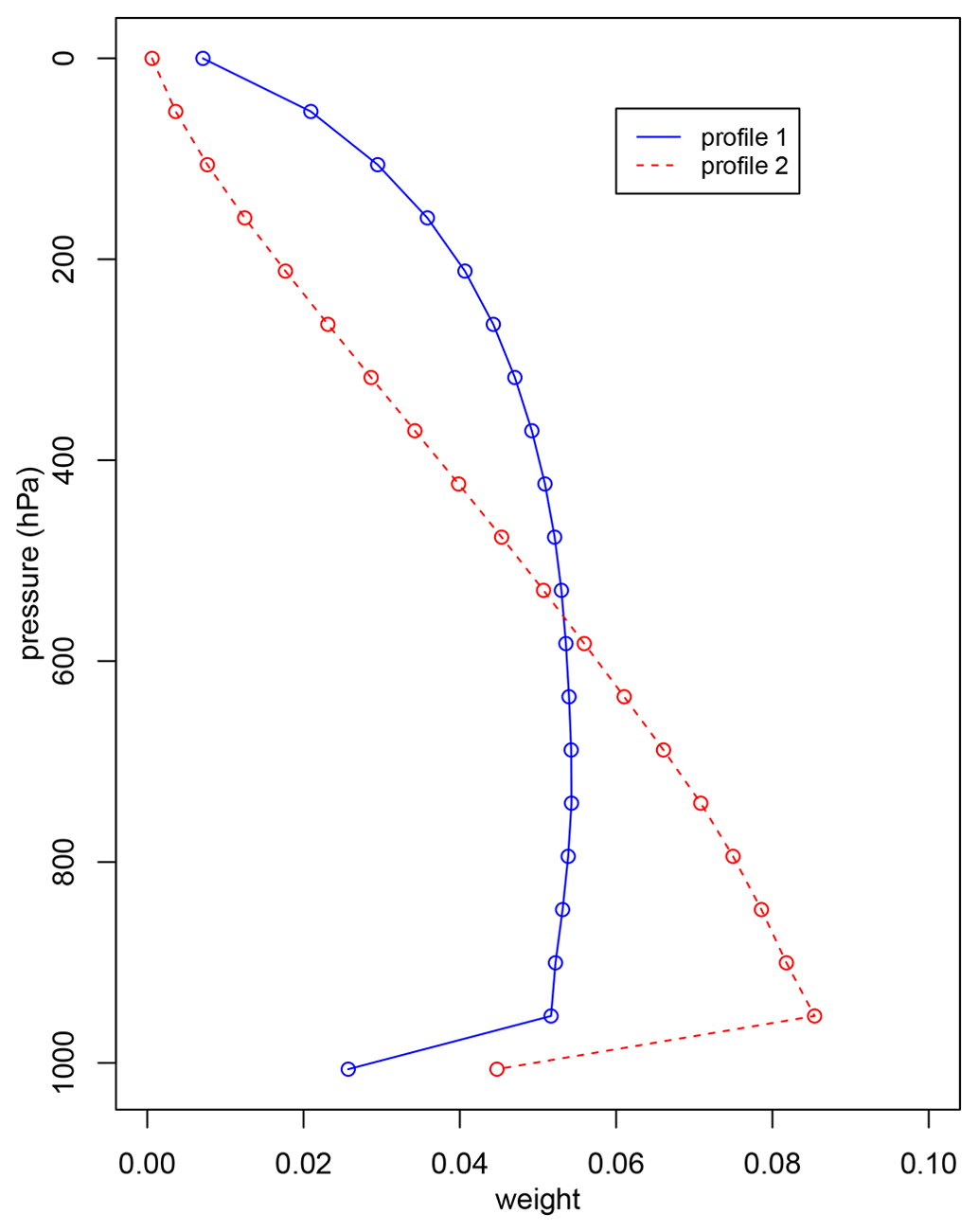
Figure 10 Two different profiles for vertically distributing a unit (ppm) of $X_{{\mathrm{CO}}_{\mathrm{2}}}$. Profile 1 is determined by OCO-2 $X_{{\mathrm{CO}}_{\mathrm{2}}}$ averaging kernel and pressure weight functions. Profile 2 is based on a redistribution of Profile 1 that gives more weight towards CO₂ in the lower troposphere than in the upper part of the atmospheric column. The circles of profiles are on the 20 pressure levels of OCO-2 $X_{{\mathrm{CO}}_{\mathrm{2}}}$ pressure weight function. Both profiles integrate to unity.

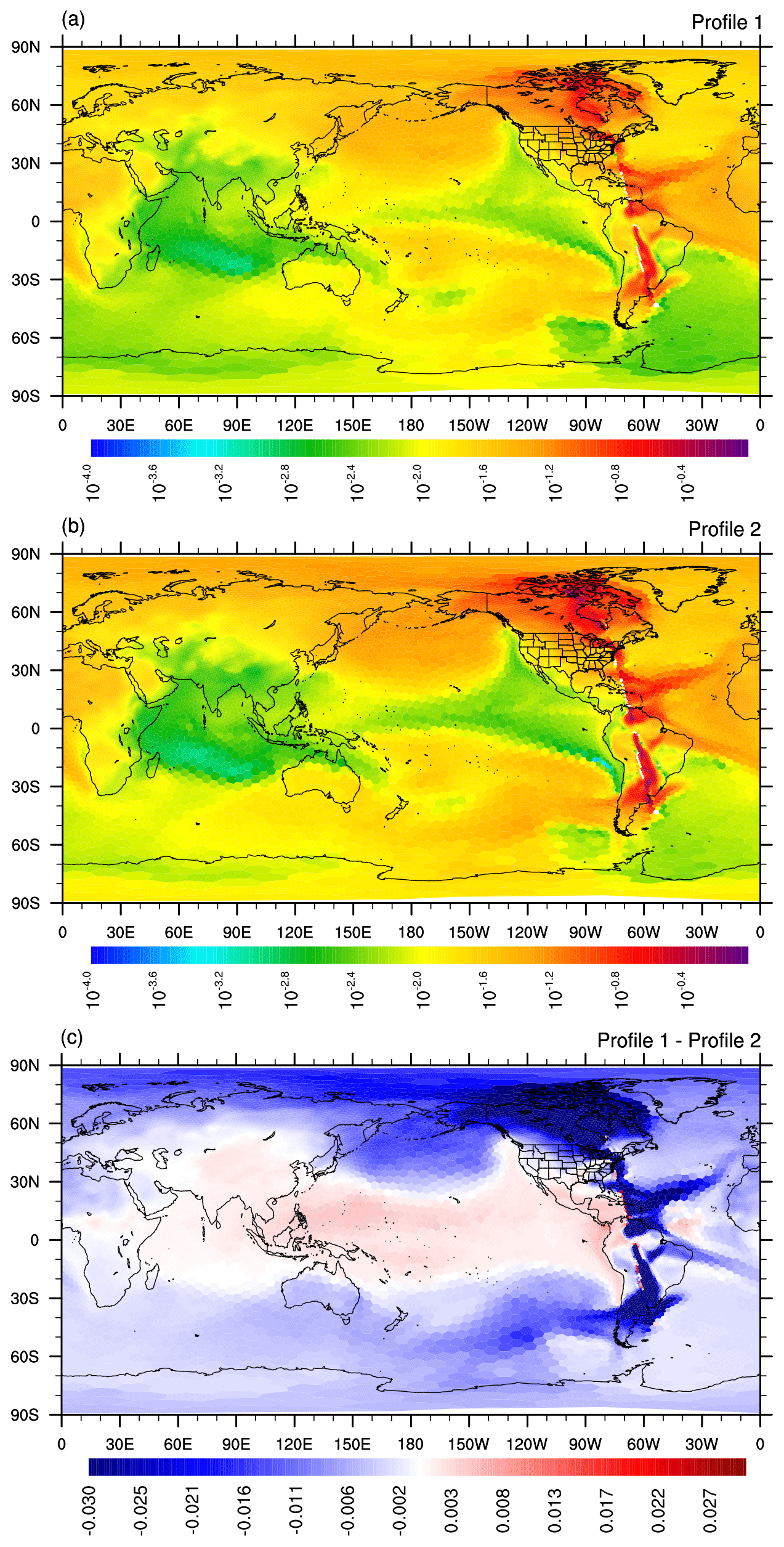
Figure 11 MPAS-CO₂ adjoint model-calculated footprints (units in $\mathrm{ppm}(\mathrm{\mu }\mathrm{mol}{\mathrm{m}}^{-\mathrm{2}}{\mathrm{s}}^{-\mathrm{1}}{)}^{-\mathrm{1}}$) obtained after 30 d of backward-in-time integration starting on 23 August 2016 at 18:00 UTC (the time of the OCO-2 measurement). The top panel (a) is obtained when using Profile 1 (Fig. 10) to vertically distribute 1 ppm of adjoint forcing. The middle panel (b) is the footprint using Profile 2. The bottom panel (c) is the difference in footprint between the two profiles.

The top two panels of Fig. 11 show the footprints resulting from MPAS-CO₂ adjoint model simulations using the two distinct vertical distribution profiles for the adjoint forcing (Fig. 10). Although the two footprints may initially appear very similar, substantial differences become evident, as shown in the bottom panel in Fig. 11. Specifically, the footprint calculated using Profile 1 exhibits lower magnitudes compared to that obtained using Profile 2 in most extratropical regions in both the Northern Hemisphere and Southern Hemisphere. Conversely, over some of the tropical regions, particularly the tropical Pacific Ocean, the footprint calculated using Profile 1 shows slightly higher magnitudes than for Profile 2. Since the two adjoint model simulations have the same meteorology, these differences in the resulting footprints might be explained by how the convective transport of CO₂ impacts the two distinctive vertical distribution profiles of the adjoint forcing. The prevalence of deep convection over the tropical Pacific Ocean can more effectively transport surface CO₂ flux to the upper atmosphere than over the extratropics, where surface CO₂ flux is more likely to be confined in the lower atmosphere. Thus, Profile 1's higher amount of adjoint forcing in the upper atmosphere results in its higher-magnitude footprint over the tropical Pacific Ocean but not over the extratropics, where its lower amount of adjoint forcing in the lower atmosphere leads to its lower-magnitude footprint. These findings underscore the critical importance of selecting an appropriate vertical distribution for the model–data difference when using an adjoint model during variational assimilation.

6 Conclusions

The MPAS-CO₂ system consists of forward, TL, and adjoint models that are built upon the variable-resolution capability of the compressible non-hydrostatic MPAS-A model (Skamarock et al., 2012). It promises to be a useful tool for carbon flux inverse modeling at the global and regional scales. The forward model of MPAS-CO₂ is documented by Zheng et al. (2021). In this paper, we focus on the development of its tangent linear and adjoint models. Through rigorous testing, we have confirmed the correctness and accuracy of the newly developed MPAS-CO₂ TL and adjoint models. A key challenge in developing the adjoint model was efficiently accessing meteorological variables during the model's backward-in-time integration. We have successfully implemented a strategy that combines recalculation and storage of meteorological variables. This approach significantly reduces the memory requirement, making the adjoint model feasible for long simulations, which are often necessary for CO₂ inverse modeling.

The results of the sensitivity analysis using the newly developed MPAS-CO₂ adjoint model provide valuable insights for designing CO₂ data assimilation systems. The increasing homogeneity of the sensitivity to the initial atmosphere CO₂ mixing ratio with longer integration length highlights the importance of selecting an appropriate assimilation window length. The comparison of the CO₂ observation footprints between the MPAS-CO₂ adjoint model and the NOAA CT-L system demonstrates good agreement, validating the accuracy of the adjoint model's footprint calculations. The comparison of OCO-2 $X_{{\mathrm{CO}}_{\mathrm{2}}}$ footprints reveals differences in sensitivity between the two systems at different altitudes. MPAS-CO₂ adjoint model-calculated footprints tend to have higher magnitudes at low altitudes and lower magnitudes at high altitudes compared to CT-L. These differences in footprints could be caused by the differences in configuration, spatial resolution, and vertical mixing processes between the two model systems. Last, the sensitivity analysis using two different vertical distribution profiles for adjoint forcing highlights the importance of correctly mapping model–data difference in X${}_{{\mathrm{CO}}_{\mathrm{2}}}$ to the transport model's vertical levels.

In addition to being a powerful tool for sensitivity analysis, the adjoint model plays a critical role in CO₂ variational data assimilation (Bosman and Krol, 2023; Tian and Zou, 2021; Zheng et al., 2018). Our future research efforts will focus on integrating the forward and adjoint models of MPAS-CO₂ into such a system. This integration has the potential to bridge a significant gap by establishing an online Eulerian-transport-model-based global variational assimilation system for CO₂ that targets high resolution in critical regions while at the same time avoiding the pitfalls associated with the lateral boundaries needed in regional domain inversions.