the Creative Commons Attribution 4.0 License.
the Creative Commons Attribution 4.0 License.
 | 20 Feb 2024
Spatial spin-up of precipitation in limited-area convection-permitting simulations over North America using the CRCM6/GEM5.0 model
François Roberge
Alejandro Di Luca
René Laprise
Philippe Lucas-Picher
Julie Thériault
A fundamental issue associated with the dynamical downscaling technique using limited-area models is related to the presence of a “spatial spin-up” belt close to the lateral boundaries where small-scale features are only partially developed. Here, we introduce a method to identify the distance from the border that is affected by the spatial spin-up (i.e., the spatial spin-up distance) of the precipitation field in convection-permitting model (CPM) simulations. Using a domain over eastern North America, this new method is applied to several simulations that differ on the nesting approach (single or double nesting) and the 3-D variables used to drive the CPM simulation. Our findings highlight three key points. Firstly, when using a single nesting approach, the spin-up distance from lateral boundaries can extend up to 300 km (around 120 CPM grid points), varying across seasons, boundaries and driving variables. Secondly, the greatest spin-up distances occur in winter at the western and southern boundaries, likely due to strong atmospheric inflow during these seasons. Thirdly, employing a double nesting approach with a comprehensive set of microphysical variables to drive CPM simulations offers clear advantages. The computational gains from reducing spatial spin-up outweigh the costs associated with the more demanding intermediate simulation of the double nesting. These results have practical implications for optimizing CPM simulation configurations, encompassing domain selection and driving strategies.
- Article
(5075 KB) - Full-text XML
- BibTeX
- EndNote


One of the greatest challenges in climate science is to produce reliable high-resolution climate information that can be used to inform impact and adaptation strategies. Global simulations performed at convection-permitting scales, with horizontal grid spacing smaller than 4 km (Satoh et al., 2019), are feasible today but remain computationally costly to produce multi-decadal climate projections and ensemble simulations. Dynamical downscaling with regional climate models (RCMs; Giorgi, 2019) using limited-area domains is a more efficient way to run at convection-permitting resolutions since the computational cost is reduced considerably compared to global convection-permitting simulations (Prein et al., 2015; Lucas-Picher et al., 2021). In recent years, several multimodel convection-permitting model (CPM) initiatives have been implemented in the context of the Coordinated Regional Climate Downscaling Experiment (CORDEX) Flagship Pilot Studies (Coppola et al., 2020; Ban et al., 2021; Mooney et al., 2022). Limited-area models must be forced at the lateral boundaries (and sometimes in the interior of the domain) by reanalysis data for hindcast studies or by simulated data generated using global or regional (with a larger domain) climate models (e.g., Earth system models, ESMs) (Laprise et al., 2008).
A remaining open key question in the regional climate modelling community relates to the specific way limited-area models are nested by global data. For a long time, it has been recognized that boundary conditions influence the limited-area model solution close to boundaries of the domain and that such influence decreases towards the interior of the domain (Rajib and Rahman, 2012; Jones et al., 1995, 1997; Seth and Rojas, 2003; Seth and Giorgi, 1998; Leduc and Laprise, 2009). As shown by Leduc and Laprise (2009), the atmospheric flow from the coarser driving simulation must travel some distance in the high-resolution limited area domain to allow enough time for the full development of the small-scale features. This distance, here denoted as the spatial spin-up distance, depends on many factors including the horizontal resolution jump between the driving and the nested model (Antic et al., 2004; Dimitrijevic and Laprise, 2005), the frequency update of the lateral boundary conditions, the selected driving variables, and the characteristics of the mean atmospheric flow, e.g., whether the flow is entering or leaving the domain (Matte et al., 2017). Using a perfect model approach (i.e., the Big Brother and idealized CPM simulations), Ahrens and Leps (2021) found that the spin-up distance of precipitation was at least 100 grid points deep along the lateral boundaries and that it could be as large as 200 grid points.
A multi-nesting approach involves employing a driving strategy in which one or multiple intermediate simulations are performed using a regional climate model between the coarse driving data (reanalysis or ESM) and the convection-permitting model (CPM) simulation. Previous studies have shown that this technique can help reduce the spatial spin-up issue (Matte et al., 2016, 2017; Cholette et al., 2015). In terms of reducing the spatial spin-up, the multi-nesting approach has three main advantages: (1) it relaxes the driving data toward the model internal dynamics/physics, (2) it reduces the horizontal (and maybe vertical) resolution jump between the driving data and the CPM simulation, and (3) it might increase the amount of information at the boundaries due to the use of a similar microphysics scheme which allows the exchange of additional variables. It should be noted that while the multiple nesting approach might offer certain advantages, whether simulations are improved compared to single nesting setups is still a subject of debate. For precipitation, Ahrens and Leps (2021) found that the use of intermediate simulations with grid spacings within the grey zone (between 2–20 km) was not advantageous compared with a single nesting using coarser resolution data. Raffa et al. (2021) also found that driving the CPM by an intermediate simulation does not improve the performance of the CPM simulation in the inner domain when looking at specific events but found similar performance for climate statistics. Additionally, according to Leps et al. (2019), the sensitivity of the performance to the jump in resolution between the nested domain and the driving data is minimal when the jump is equal to or below 6.
The objective of this study is twofold. First, we develop a method to diagnose the spatial spin-up of convection-permitting simulations, focusing on the precipitation fields simulated by the model and those obtained from the driving fields (ERA5 reanalysis data or the intermediate simulations). Second, we use the spatial spin-up diagnostic to assess different driving strategies. Several driving strategies are considered including the use of intermediate simulations (double nesting) and the use of different variables to drive the convection-permitting model, sometimes including microphysical variables in the driving fields. The analysis of the driving strategies includes an assessment of the total computational cost (storage and running costs) of simulations to put in perspective the advantages and disadvantages of each driving strategy.
The paper is organized as follows: descriptions of the data and the model used are included in Sect. 2.1 and 2.2, respectively, while a description of the experimental design of simulations is provided in Sect. 2.3. In Sect. 3, we describe how the spatial spin-up diagnostic is calculated, its application to simulations using different driving strategies and a discussion about the implications of our results for computing resources. A summary and conclusions are given in Sect. 4.
2.1 The ERA5 reanalysis
ERA5 (Hersbach et al., 2020) is the latest reanalysis produced by the European Centre for Medium-Range Weather Forecasts. ERA5 is produced by assimilating observations from different types and sources into the Integral Forecasting System Cycle 41r2 model, which has a horizontal grid spacing of about 31 km and 137 model levels up to 0.01 hPa. ERA5 variables are also made available on a latitude–longitude grid with spacing of 0.25∘ and interpolated into 37 pressure levels from 1000 up to 1 hPa at hourly intervals. We use temperature, geopotential height, horizontal winds and specific humidity at all 37 pressure levels to drive our simulations. In addition, daily values (instantaneous values at 12:00 Z) of sea surface temperature and sea ice fraction are also used to force the model at the surface.
2.2 The CRCM6/GEM5.0 model
In this study, we use the sixth generation of the Canadian Regional Climate Model (CRCM6/GEM5.0), which is currently being developed at the ESCER (Étude et simulation du climat à l'échelle régionale) center at UQAM (Université du Québec à Montréal). The CRCM6/GEM5.0 version used here is based on version 5.0.2 of the Global Environmental Multiscale model (GEM5) (McTaggart-Cowan et al., 2019b), which is the operational numerical weather prediction model used by the Meteorological Service of Canada.
Two configurations of the CRCM6/GEM5.0 model are used in this study and differ in their horizontal resolution and the choice of some parameterizations (see Table 1). The first configuration, denoted as GEM12, uses a horizontal grid spacing of 0.11∘ (about 12 km) and is run over the CORDEX North American domain (Giorgi and Gutowski, 2015) (see the green domain in Fig. 1). For this large North American domain, large-scale spectral nudging is applied to horizontal winds and temperature variables. Spectral nudging is applied for levels higher than the 0.85 hybrid level (which corresponds to about 850 hPa) and for horizontal scales greater than 200 km using a relaxation timescale of 8 h.
A second configuration of the model, denoted as GEM2.5, is run in convection-permitting mode using a horizontal grid spacing of 0.0225∘ (about 2.5 km). This configuration is run over a domain centered over southern Quebec, Canada, that covers a large part of northeastern North America (see the blue domain in Fig. 1).
Table 1Key features of the two model configurations (GEM12 and GEM2.5) employed in this study.
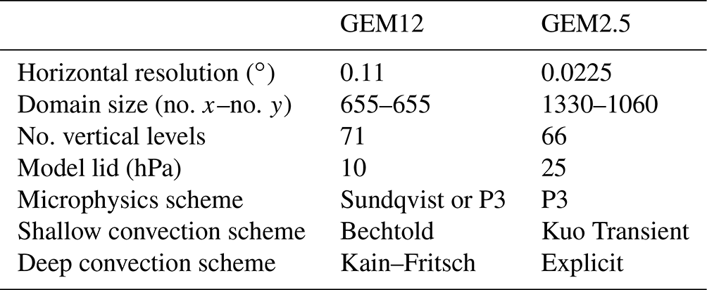
GEM12 can produce precipitation in two ways, i.e., through the Kain–Fritsch deep convective scheme (Kain and Fritsch, 1990; McTaggart-Cowan et al., 2019a) and by explicitly condensating water vapour at the grid scale. While GEM12 uses a shallow convection scheme (Bechtold et al., 2001), this does not produce precipitation. GEM2.5 also produces precipitation in two ways, through the Kuo Transient shallow convection scheme (Bélair et al., 2005) and by explicitly condensating water vapour as the deep convective parameterization scheme is turned off. To condensate and create hydrometeors at the grid scale, two schemes are available in the GEM12 model framework: a simple condensation scheme (Sundqvist et al., 1989) and a more sophisticated microphysics scheme called P3 (Morrison and Milbrandt, 2015; Morrison et al., 2015; Milbrandt and Morrison, 2016). The Sundqvist scheme uses a single prognostic variable that represents a cloud water/ice category, while P3 uses a total of eight prognostic variables, four prognostic variables for the liquid phase and four prognostic variables for the solid phase with multiple types of hydrometeors. When using the GEM2.5 model, only the P3 microphysics scheme is used. To improve the sensitivity of P3 to the model resolution, all simulations use a subgrid cloud and precipitation fraction scheme that was recently developed (Chosson et al., 2014; Jouan et al., 2020).
GEM12 and GEM2.5 use version 3.6 of the Canadian Land Surface Scheme (CLASS) (Verseghy, 2000, 2012) with 16 soil layers down to a maximum depth of 10 m. An earlier version of CLASS has been used in a number of studies with the fifth-generation of the Canadian Regional Climate Model (CRCM5) (Zadra et al., 2008; Lucas-Picher et al., 2017; Martynov et al., 2013). In addition, all simulations use the Fresh-water Lake (FLake) model (Martynov et al., 2012; Mironov et al., 2010) to represent lake surface temperatures.
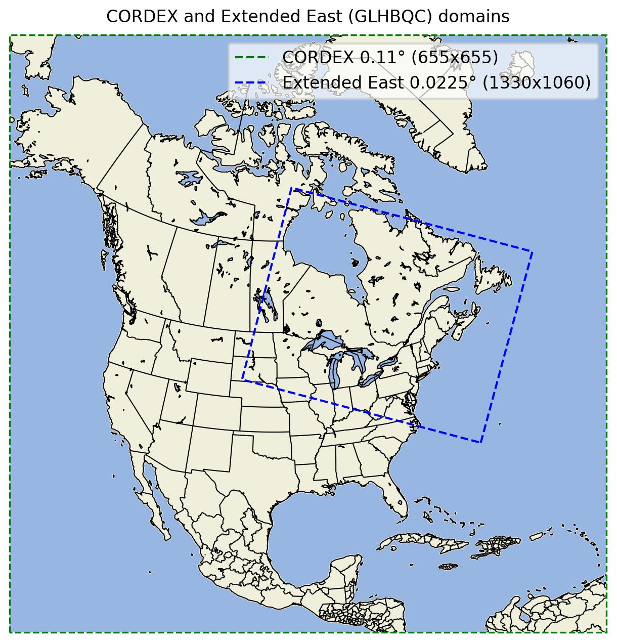
Figure 1Domains used for the GEM2.5 simulations (blue square) and GEM12 simulations (green square). Domains shown do not include grid points in the relaxation or blending zone.
2.3 Experimental design of simulations
Seven simulations were performed using the convection-permitting version of the model (GEM2.5) to evaluate the sensitivity of the spatial spin-up to the driving strategies. Figure 2 presents the different driving strategies. A first GEM2.5 simulation, denoted as GEM2.5 (ERA5), is driven at the boundaries using pressure-level standard driving variables (SDVpres) from the ERA5 reanalysis. SDVpres includes horizontal wind components, temperature, geopotential height and specific humidity on 37 pressure levels. A second GEM2.5 simulation, denoted as GEM2.5 (SU), is driven by a GEM12 simulation performed using the simple condensation scheme of Sundqvist (GEM12_SU (ERA5)) and the hybrid model-level standard driving variables (SDVhybr). SDVhybr variables in the GEM12 case are different from those used with ERA5 as they include horizontal wind components, temperature and specific humidity on 71 model levels, and the orography (geopotential height at the surface). A third GEM2.5 simulation (SU-W) is the same as the previous one, but the vertical velocity from the GEM12_SU (ERA5) simulation is also included in the driving data. In addition, four other GEM2.5 simulations were performed using a GEM12_P3 (ERA5) simulation at the boundaries:
-
GEM2.5 (P3-C), driven at the lateral boundaries by the SDVhybr and the 3-D liquid cloud hydrometeors (liquid cloud mass mixing ratio (qc (kg kg−1)) and liquid cloud number mixing ratio (Nc (no. kg−1) from GEM12_P3 (ERA5);
-
GEM2.5 (P3-CR), the same as (1) with the addition of the 3-D rain hydrometeors (mass rain mixing ratio (qr (kg kg−1)) and rain number mixing ratio (Nr (no. kg−1)));
-
GEM2.5 (P3-CRI), the same as (2) with the addition of 3-D ice hydrometeors (total ice mass mixing ratio (qi,tot (kg kg−1)), rime mass mixing ratio (qi,rim (kg kg−1)), total ice number mixing ratio (Ni,tot (no. kg−1)) and rime volume mixing ratio (Bi,rim (m3 kg−1)));
-
GEM2.5 (P3-WCRI), the same as (3) with the addition of the 3-D vertical speed (actual model vertical velocity (wreal (m s−1)) and coordinate vertical velocity (wcor)).
All four GEM2.5 (P3-xxx) simulations described above are driven by the same GEM12_P3 (ERA5) simulation but read different variables at the lateral boundary conditions, with GEM2.5 (P3-WCRI) being driven by the full set of 3-D dynamical, thermodynamical and microphysical variables.
All our GEM simulations use a Newtonian relaxation scheme of 10 grid points to constrain all GEM-simulated prognostic variables v in the neighbourhood of the boundaries toward the externally prescribed field (Davies, 1976). In particular, in the relaxation zone (sometimes denoted as sponge zone), a term of the form ) is added to the prognostic equations. In our formulation, the weights K follow a cosine-squared profile, which decreases from a value of 1 in the outside to a value of zero in the inside of the relaxation zone. In addition, an extra 10 grid points are used for the calculation of semi-Lagrangian trajectories. Furthermore, GEM2.5 or GEM12 simulations are driven from the top, with a lid at 25 and 10 hPa, respectively. All simulations were initialized on 1 September 2015, and the analysis was performed for the period between 1 December 2015 and 30 November 2017 (2 years are used for each season).
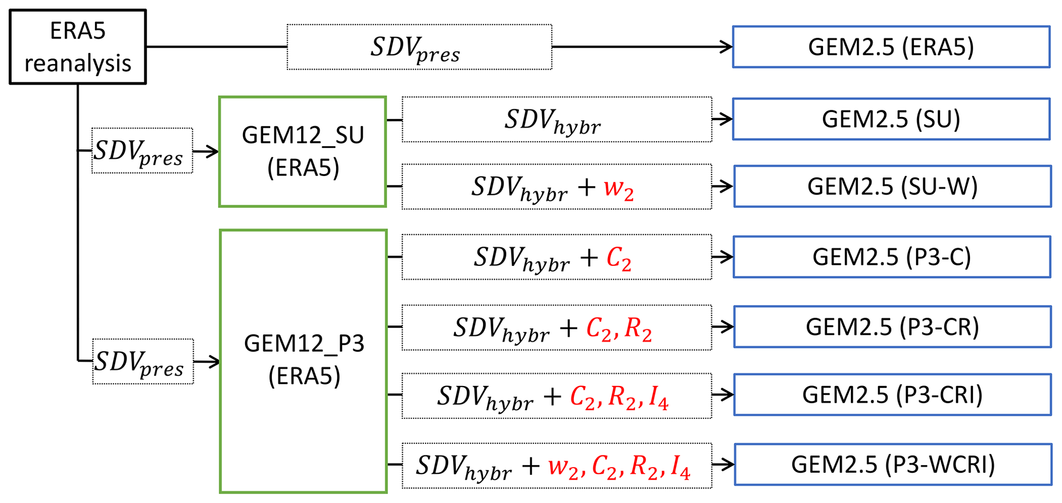
Figure 2Schematic presentation of the various driving strategies used to generate the spatial spin-up ensemble of simulations. Standard driving variables (SDV_pres and SDV_hybr) refer to the minimum set of variables that are necessary to run GEM2.5 simulations using pressure and hybrid vertical levels and are specified in the text (see Sect. 2.3). Other variables used to drive GEM2.5 are actual and coordinate vertical velocities (w2), two liquid cloud variables (C2), two liquid precipitation variables (R2), and four ice hydrometeor variables (I4). See the text for more details about microphysics variables.
3.1 Spatial spin-up distance (SSUD) diagnostic
A spatial spin-up diagnostic (SSUD) is proposed here to quantify the spatial spin-up at each boundary (eastern, western, northern and southern boundaries) for different seasons. Estimating SSUD requires several steps that are described below. First, let us denote the time average precipitation at each grid point (i,j) by pi,j, with i varying between 0 and Ni−1 (domain size in the x direction) and j varying between 0 and Nj−1 (domain size in the y direction). Top panels in Fig. 3 show DJF fields of pi,j for ERA5 and GEM12_P3 (ERA5), and bottom panels show pi,j for the two simulations GEM2.5 (ERA5) and GEM2.5 (P3-WCRI). All four fields show similar large-scale patterns of mean precipitation, with a general increase towards the east of the domain and a maximum over the Atlantic Ocean. While GEM2.5 precipitation fields (bottom row) present higher fine-scale variability, which may be considered part of the added-value of finer resolution, lower precipitation along some of the boundaries, particularly over the southern boundary, is clearly a defect from the lateral spin-up.
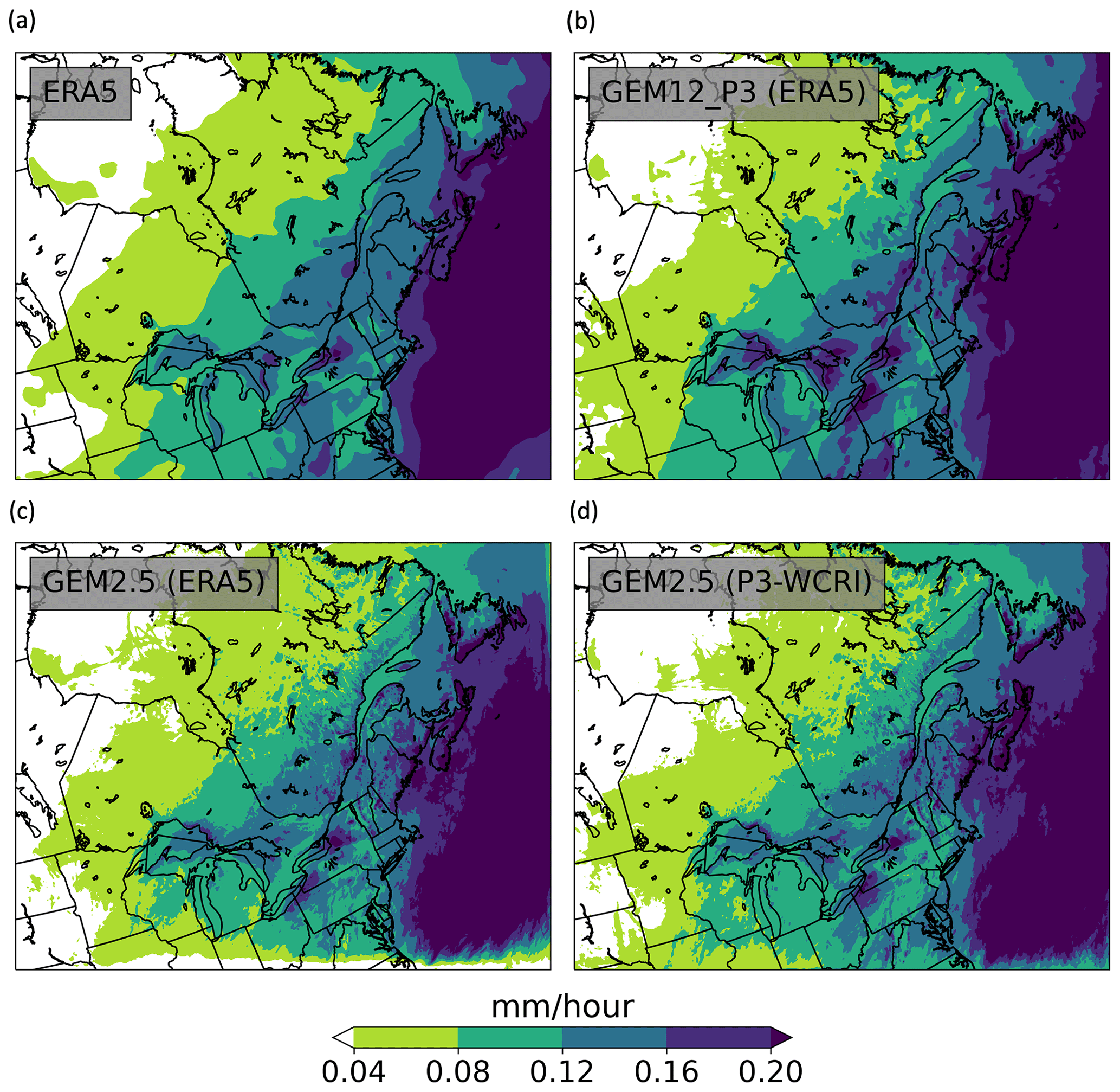
Figure 3Winter (DJF) mean precipitation rate over the GEM2.5 domain for (a) ERA5, (b) GEM12_P3 (ERA5), (c) GEM2.5 (ERA5) and (d). GEM2.5 (P3-WCRI),
To quantify the artifacts created by the GEM2.5 simulation close to the boundaries, we calculate the average of the mean precipitation field pi,j in the meridional and the zonal directions:
where A=0.25. Excluding a ribbon of width equal to a quarter of the domain around the perimeter prevents the zonal and meridional averages from being contaminated by the spatial spin-up in the other direction. In addition, to account for the fact that the mean precipitation rate can be different for different products, the zonal and meridional averages are normalized by the domain- and time-averaged precipitation rate :
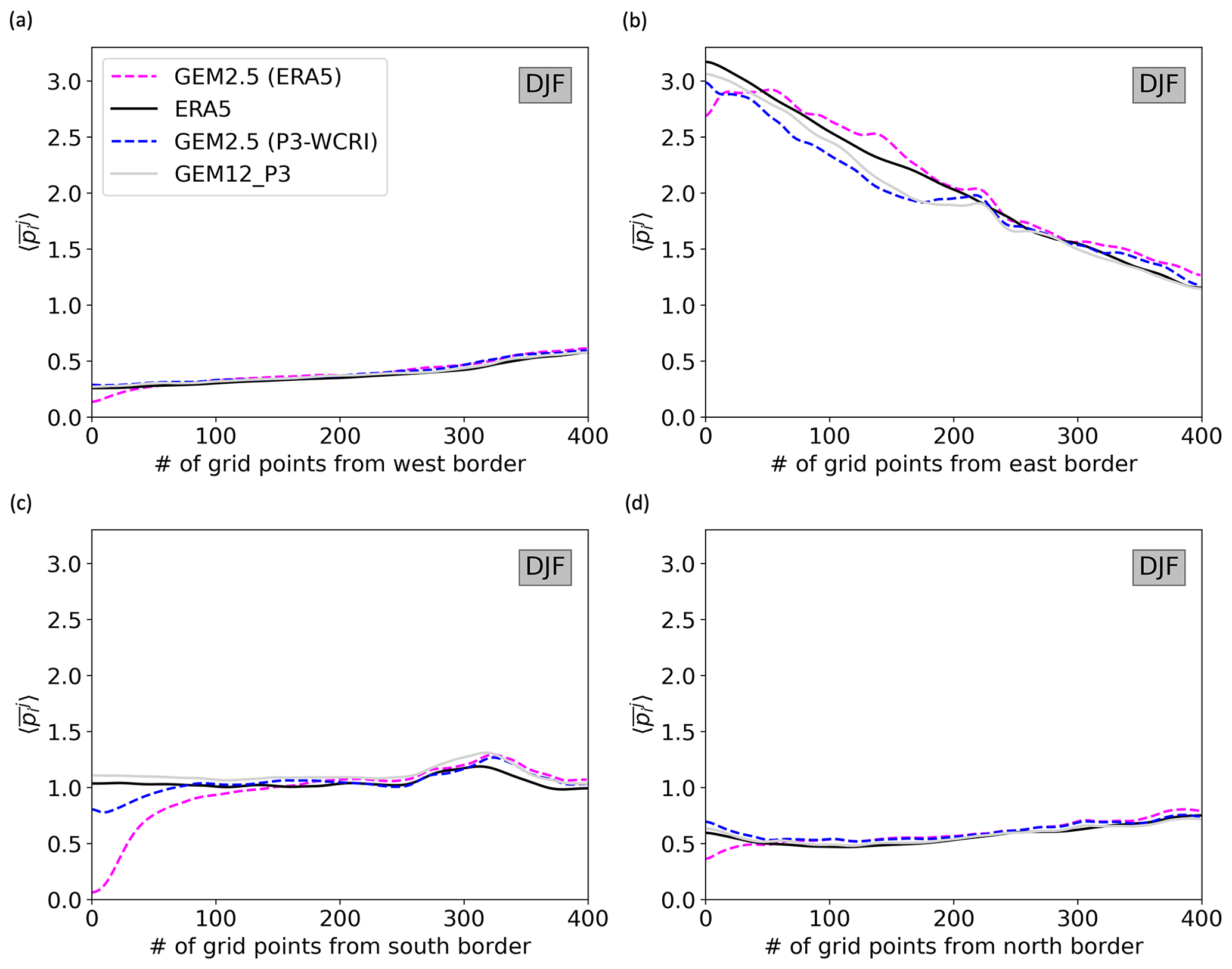
Figure 4Average of the mean precipitation field in (a) and (b) the meridional directions and (c) and (d) the zonal directions for GEM2.5 (ERA5) and GEM2.5 (P3-WCRI) simulations and the corresponding driving data ERA5 and GEM12_P3 (ERA5). Each panel shows results for a different boundary driving. Eastern and northern boundaries have been mirrored, so the grid point 0 always denotes the grid point closest to the boundary.
Figure 4 shows and for GEM2.5 (ERA5) and GEM2.5 (P3-WCRI) simulations and their corresponding driving data within 400 grid points from each boundary. The north and east boundaries have been mirrored, so the zeroth grid point always denotes the first grid point from the boundary. In addition, a Gaussian filter with a sigma equal to 5 grid points has been used to smooth the fine-scale precipitation variability. This implies that the minimum spin-up distance identified by the algorithm is about five grid points. In general, GEM2.5 simulations closely follow the driving data away from the boundary, but significant differences can be observed near the boundaries. This is especially noticeable for some boundaries (e.g., south border). It is also clear that the simulation GEM2.5 (ERA5) that is directly driven at the boundaries by the ERA5 reanalysis shows larger deviations from its driving data than the simulation GEM2.5 (P3-WCRI) that uses a full set of microphysical variables as driving fields.
The differences between and as obtained from the GEM2.5 simulation and the driving data can be used to estimate the SSUD. In particular, the relative difference (RD) between from a GEM2.5 simulation and the corresponding driving data can be calculated as follows:
Figure 5 shows that, away from the boundaries, the relative differences fluctuate around 0, although the mean value () may deviate slightly from 0. We estimate the variability of the relative difference by computing its standard deviation far from the boundary so that the variability is not contaminated by the spin-up. Arbitrarily, we assume that the spin-up distance is smaller than 133 grid points (corresponding to 33 % of the 400 grid points considered), and the standard deviation of the relative difference (σ(RD)) is calculated using grid points between 133 and 400. Values of are shown using a shaded coloured area. The SSUD is then determined as the largest distance away from the boundary for which the mean relative difference () is lower than 2.5 ⋅σ(RD) from the mean relative difference. The SSUD values are shown in Fig. 5 using large dots. If the relative difference has a Gaussian distribution, then the choice of 2.5 ⋅σ(RD) implies that the SSUD would be incorrect in only 0.3 % cases.
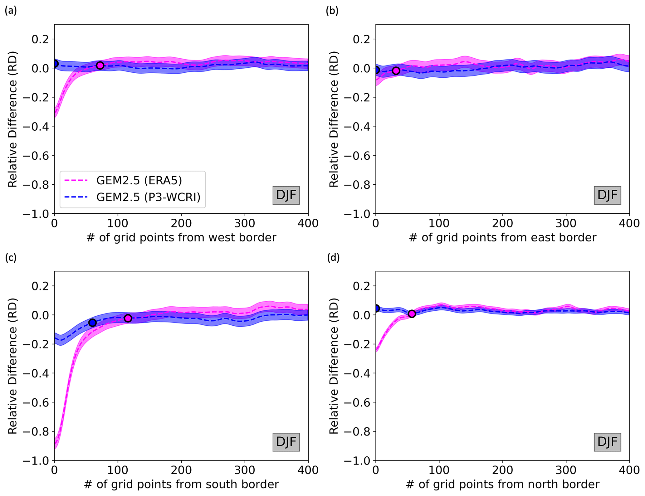
Figure 5Mean precipitation relative difference (RD) between GEM2.5 simulation and the corresponding driving data for (a) and (b) the zonal averages and (c) and (d) the meridional averages (dotted lines). Dashed lines show 2 times the standard deviation of the uncontaminated relative difference RD. Dots show the estimated SSUD in each case. Values of are shown using full lines. The SSUD values are shown using large dots.
For the GEM2.5 (ERA5) simulation, we obtain SSUD values of 72, 32, 116 and 60 grid points for the west, east, south and north boundaries, respectively. For the GEM2.5 (P3-WCRI) simulation, we obtain SSUD values of 0, 0, 60 and 0 grid points for the west, east, south and north boundaries, respectively. These results align well with a visual examination of Fig. 4. Since several parameters such as the total distance from the boundary, the free spin-up distance and the number of standard deviations from the mean are selected arbitrarily, Sect. 3.4 assesses the sensitivity of the algorithm to the choice of these parameters.
3.2 Dependence of SSUD on the driving strategy
Figure 6 shows that SSUD values depend strongly on the season, the boundary and the simulations and vary between 0 and 116 grid points. Differences between GEM2.5 (SU) and GEM2.5 (SU-W) are generally very small for all seasons and borders. GEM2.5 (SU-W) and GEM2.5 (SU) SSUD values are sometimes larger than GEM2.5 (ERA5) values. As an example, in MAM at the west boundary, GEM2.5 (ERA5) has a SSUD of 26 points, GEM2.5 (SU) has a SSUD of 97 points and GEM2.5 (SU-W) has a SSUD of 101 points. On average, however, simulations driven by GEM12_SU (ERA5) show lower SSUD values than those driven directly by ERA5 (e.g., in DJF).
Interestingly, GEM2.5 (P3-C) and GEM2.5 (P3-CR) always have similar SSUD values to each other. They are often, but not always, lower than SSUD values obtained from GEM2.5 (SU) and GEM2.5 (SU-W) (see for example the north boundary for DJF and MAM).
Results show that both simulations that are driven by ice hydrometeor variables (GEM2.5 (P3-CRI) and GEM2.5 (P3-WCRI)) have consistently lower SSUD values than all other simulations. In DJF, only the south boundary shows non-negligible SSUD values for GEM2.5 (P3-CRI) and GEM2.5 (P3-WCRI) (SSUD is about 60 grid points). In MAM, SSUD values are generally small except for the west boundary, with SSUD values of 19 and 24 grid points, and for the south boundary, with SSUD values of 27 grid points for both simulations. In SON, only the south boundary has a SSUD of around 27 grid points. In JJA, all simulations show low SSUD values except for GEM2.5 (ERA5) that shows a SSUD value of 83 grid points for the west boundary.
The addition of vertical velocities to the driving fields seems to have a negligible effect on SSUD values, as demonstrated by the small differences between GEM2.5 (SU) and GEM2.5 (SU-W) and between GEM2.5 (P3-WCRI) and GEM2.5 (P3-CRI). These results indicate that passing all eight microphysical variables from P3 (CRI) to the nested domain implies a much higher benefit than passing the vertical wind speed velocities (W).
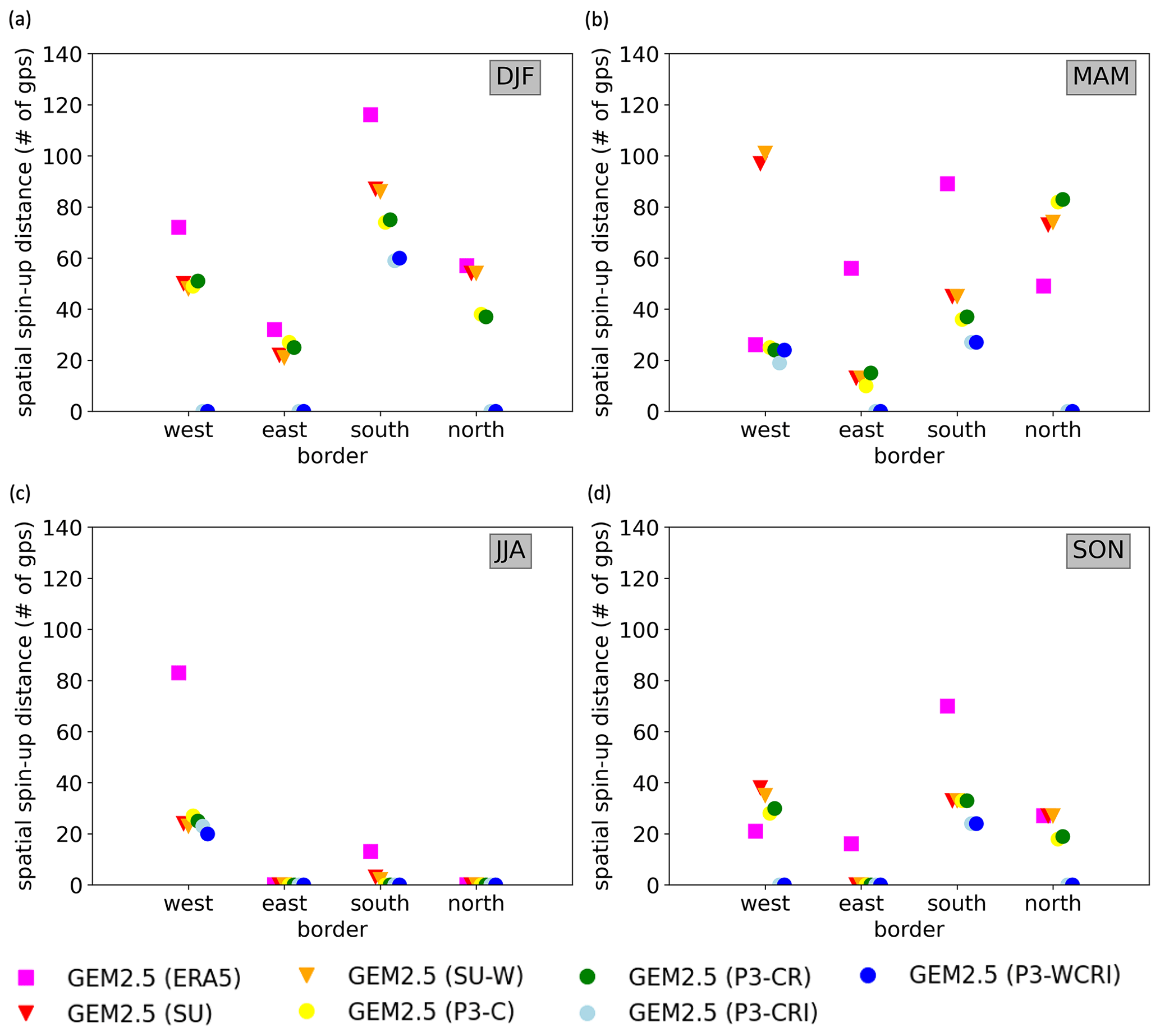
Figure 6SSUD estimated for different boundaries, seasons and all members of the spatial spin-up ensemble driving strategy. SSUD is expressed in kilometres.
3.3 Seasonal and boundary dependence of SSUD
Figure 7 summarizes previous results by showing mean SSUD values across different boundaries and different seasons for individual simulations. As noted earlier, SSUD values depend strongly on the driving strategy, the season and the boundary. Averaged SSUD values across seasons and boundaries vary between 0 and about 70 grid points. The largest SSUD values are observed at the southern and western boundaries, followed by the northern and eastern ones. For the seasonal mean values, the largest values are obtained in winter followed by fall, spring and summer. The SSUD generally decreases as more microphysical variables are included in the driving fields, leading to the largest SSUD values for the GEM2.5 (ERA5) simulation and the lowest for the GEM2.5 (P3-WCRI) simulation.
According to Fig. 7, the mean SSUD value remains unchanged despite the addition of certain variables in the driving data. Specifically, using a double nesting with the Sundqvist condensation scheme GEM2.5 (SU) and GEM2.5 (SU-W) does not always decrease the SSUD value compared with the single nesting using ERA5. Similar results are obtained when using cloud (GEM2.5 (P3-C) and rain hydrometeors (GEM2.5 (P3-CR)), while the addition of vertical velocities affects the SSUD values little (e.g., GEM2.5 (P3-CRI) vs. GEM2.5 (P3-WCRI)). The largest reduction in SSUD values occurs when ice hydrometeors are included as GEM2.5 (P3-CRI) systematically leads to lower SSUD than the GEM2.5 (P3-CR) simulation.
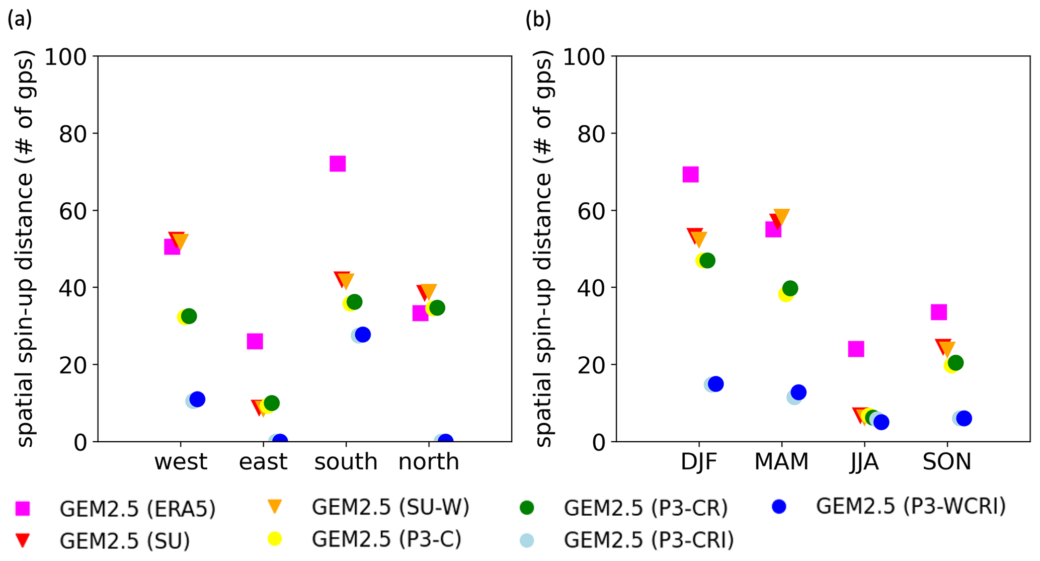
Figure 7SSUD estimated for different boundaries and different seasons for the GEM2.5 (ERA5) and the GEM2.5 (GEM12_P3-WCRI) simulations. The SSUD is expressed in kilometres from the boundary.
3.4 Sensitivity of SSUD calculation
The estimation of the SSUD diagnostic depends on several parameters, and its sensitivity is evaluated here. Figure 8a shows SSUD values as estimated using different choices of parameters for the number of standard deviations from the mean (1.5σ, 2.5σ and 3.5σ) and the percentage of the distance without spin-up (25 % and 33 %) as a function of the total number of grid points from the boundary. SSUD values depend strongly on the number of standard deviations, with mean values around 38 grid points for 3.5σ and about 60 grid points for 1.5σ. For 2.5σ and 3.5σ, SSUD mean values depend little on the total number of grid points and the assumed distance without spin-up.
Figure 8b shows the ratio of SSUD values between the GEM2.5 (ERA5) and the GEM2.5 (P3-WCRI) simulation. For 2.5σ and 3.5σ, the ratio takes values between 0.25 and 0.2 and tends to slightly decrease as the total number of grid points increases from 300 to 500. SSUD values appear to be highly sensitive to the choice of the total number of grid points when using 1.5σ, suggesting that the 1.5σ value might be too low a threshold.
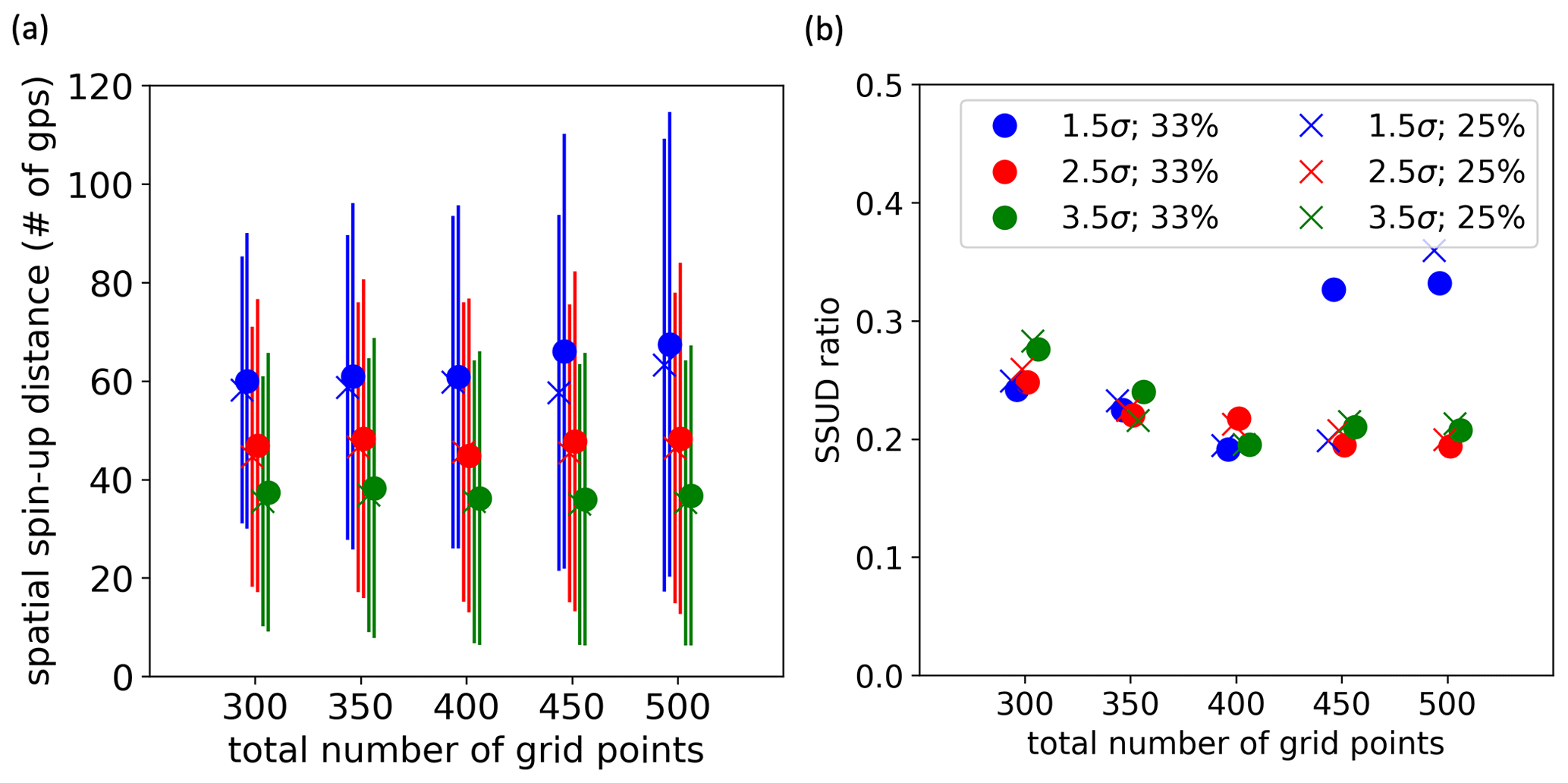
Figure 8Panel (a) shows SSUD mean values (± one standard deviation) as estimated using different choices of parameters for the number of standard deviations from the mean (σ), the percentage of the distance with no spin-up (25 % and 33 %) as a function of the total number of grid points from the boundary. Panel (b) shows the ratio of SSUD between the GEM2.5 (ERA5) and the GEM2.5 (P3-WCRI) simulation.
3.5 Implications of the spatial spin-up for computing resources
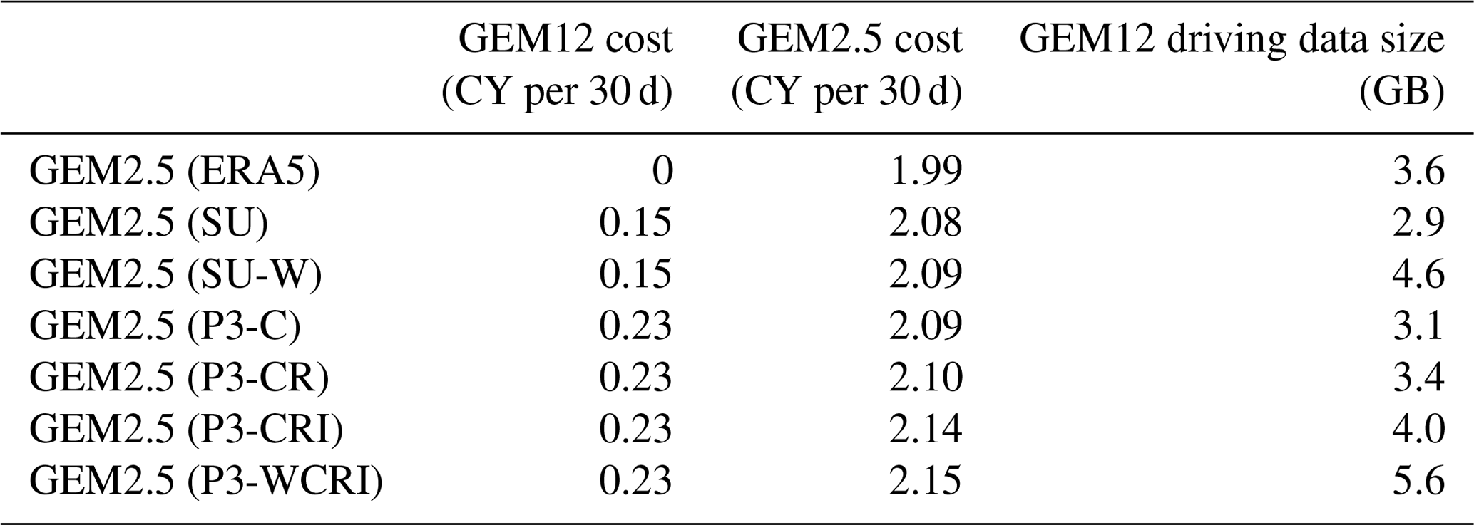
Several GEM2.5 simulations with different driving strategies have been considered in this study. While all simulations are performed using the same GEM2.5 model configuration (i.e., same vertical and horizontal resolution and domain size), their effective computational costs vary depending on two factors: (1) the full cost of the GEM2.5 simulation including the cost of running the intermediate simulation to generate all the driving data and (2) the reduction of the effective domain due to the spatial spin-up. The computational cost of running simulations is shown in Fig. 9 and Table 2. Furthermore, the third column in Table 2 indicates the disk space required for storing the driving fields, which could also pose a constraint and escalates significantly with the number of 3D prognostic variables.
As we are interested in comparing the relative costs of simulations, computational costs are normalized by the cost of the GEM2.5 (ERA5) simulation. As expected, the least expensive simulation is the one directly driven by the ERA5 reanalysis, which does not require an additional simulation using the GEM12 model. The computational costs of the GEM2.5 simulations driven by GEM12 fields increase as the complexity of the GEM12 increases because GEM12 becomes more computationally demanding (GEM12_P3 (ERA5) is 50 % more expensive to run than GEM12_SU (ERA5) due to the more complex microphysical scheme) but also because GEM2.5 is computationally more expensive when additional variables must be read at the boundaries. Overall, a double-nesting approach increases the cost by about 12 % when driven by GEM12_SU (ERA5) and by about 20 % when driven by GEM12_P3 (ERA5). Furthermore, the cost does not depend on the choice of the season but rather on the size of the domain and the complexity of the 12 km simulation. In our case, the 12 km domain is rather large as it corresponds to the North American CORDEX domain, and it could be reduced in the case that GEM12 simulations are only performed to produce boundary conditions for the GEM2.5.
Table 2Computational cost of GEM12 and GEM2.5 simulations in core years (CY) per 30 simulated days. The third column also includes the size (in GB) of the driving data for each simulation.
The presence of spatial spin up implies that a part of the GEM2.5 domain provides unrealistic precipitation and must therefore be excluded in the final analysis. For each simulation, we can use the SSUD values to calculate the effective number of grid points where precipitation is not affected by spatial spin-up artifacts as follows:
As expected, the largest fraction is obtained when considering GEM2.5 (P3-CRI) and GEM2.5 (P3-WCRI) for which more than 94 % of the domain is not affected by spin-up artifacts (Fig. 9). The fraction of the domain decreases to about 75 % in the case of the GEM2.5 (ERA5) simulation in winter.
Finally, the cost per effective grid point shows that, except for DJF, the least expensive simulation is the one that is directly driven by the ERA5 reanalysis because no additional simulation is needed (Fig. 9). Except for JJA, the second-most-efficient simulations are those including ice hydrometeors GEM2.5 (P3-WCRI) and GEM2.5 (P3-CRI). Indeed, for most seasons, the decrease in the spatial spin-up is compensated for by the cost of running the additional GEM12_P3 (ERA5) model. As expected, the gain of using a full set of microphysics variables is the largest for the seasons with the largest spatial spin up.
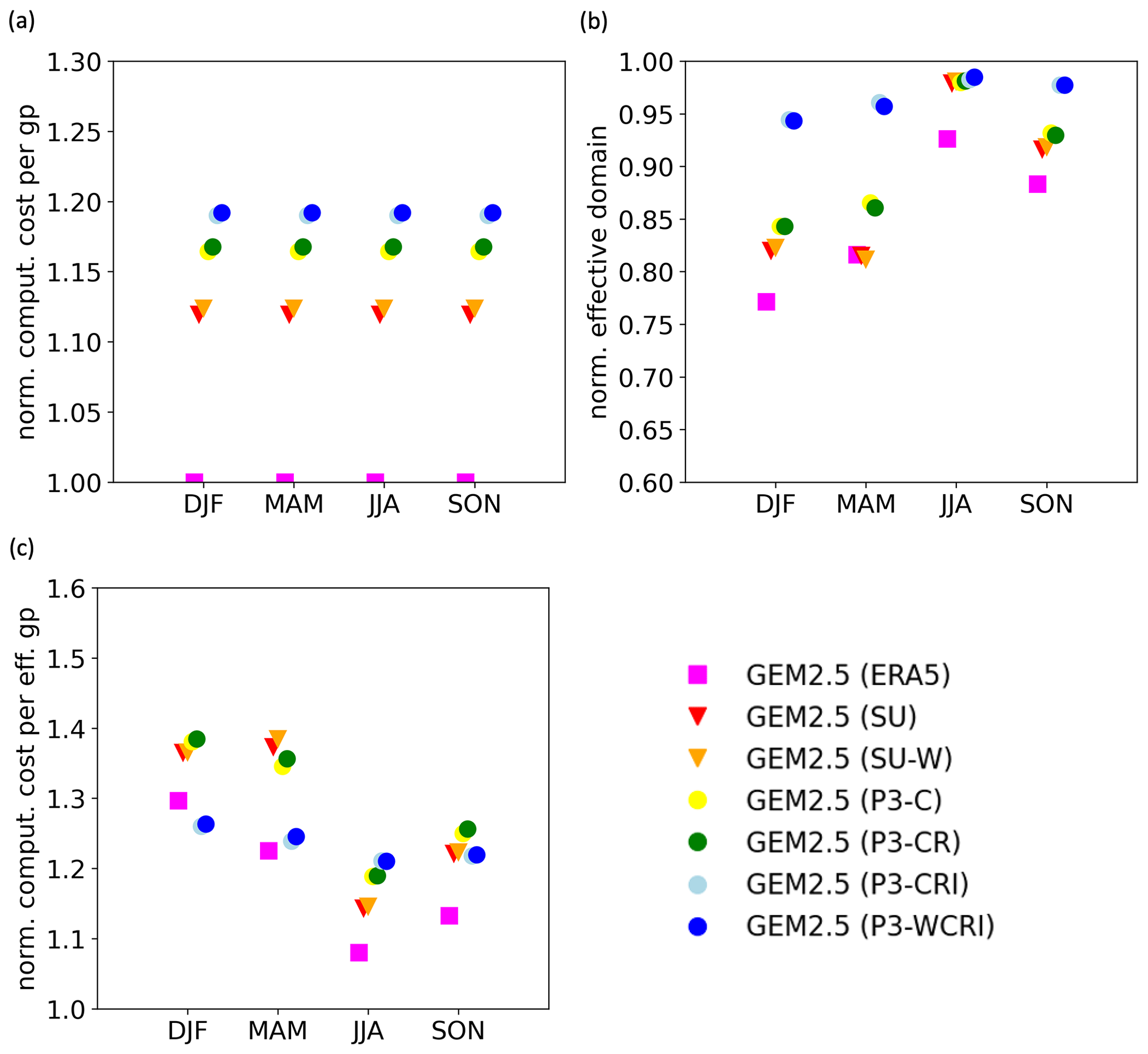
Figure 9(a) The computational costs of simulations, normalized by the cost of the GEM2.5 (ERA5) simulation. (b) The normalized effective domain estimated as the fraction of grid points that is not affected by the spatial spin up. (c) The combined effect of the computational cost and the effective domain estimated as the ratio between the normalized computational cost per grid point and the normalized effective domain.
Using limited-area domains, the dynamical downscaling technique provides a cost-effective way of producing high-resolution climate information with regional climate and convection-permitting models (RCMs and CPMs) compared with global climate models. However, limited-area domain simulations suffer from spatial spin-up artifacts close to the domain boundaries where the low-resolution driving data are relaxed towards the higher-resolution model. In this paper, a spatial spin-up diagnostic (SSUD) estimating the distance from the boundary for which these artifacts are located was introduced using the precipitation variable. The SSUD was applied to an ensemble of simulations that uses different driving strategies for identifying the optimal driving strategy of CPM simulations.
The results showed that the SSUD depends strongly on the boundary and season, confirming previous results that suggested a strong dependence of the spatial spin-up on the atmospheric flow characteristics (Leduc and Laprise, 2009; Matte et al., 2017). Specifically, for the CPM simulation driven at the boundaries directly by the ERA5 reanalysis, SSUD ranged from about 120 grid points (i.e., about 300 km) for the southern boundary in DJF to close to zero for the eastern/northern boundaries in JJA. This result is consistent with the findings by Ahrens and Leps (2021) that found SSUD values between 100 and 200 grid points when using idealized CPM simulations and a perfect model approach for the estimation of the SSUD.
Regardless of the CPM simulation, the seasonal dependence of SSUD shows that the largest values are found in DJF, followed by MAM, SON and JJA. These results are consistent with Matte et al. (2017), which showed much higher values in winter than in summer, relating the differences with the strength of horizontal wind speeds for different seasons. Moreover, the results indicated that the SSUD is larger over the western and southern boundaries compared to eastern and northern boundaries. This is consistent with the western and southern boundaries being regions where the atmospheric flow enters the domain most of the time (Leduc and Laprise, 2009). Given these results, it seems that a minimum of 50 grid points should be removed at the inflow boundaries prior to analysis of the precipitation field for mid-latitude CPM experiments that use a single-nesting approach. The SSUD depends on the choice of driving strategy. The SSUD decreases drastically when 3-D ice hydrometeors are used at the boundaries. The inclusion of vertical wind speed in the 3-D driving variables has no effect on the SSUD. Adding the 3-D liquid cloud/rain hydrometeors to the driving variables generally decreases SSUD values that remain dependent on the season and boundary.
Two aspects of the computational costs of our simulations were assessed. First, we estimated the computational gain associated with a decrease in the spatial spin-up (cost per effective grid point). Second, we estimated the computational loss associated with the use of intermediate simulations. The least expensive simulation per “effective grid point” is the one using a single nesting that is directly driven by the ERA5 reanalysis, while the next least expensive simulations are the ones using the eight microphysical variables at the boundaries. These results demonstrate that when using all hydrometeors to drive the CPM, the effect of decreasing the spatial spin-up exceeds the effect of using an intermediate simulation. Among the two simulations using all hydrometeors, the optimal configuration would be the one without the vertical velocity at the boundaries because it increases by 40 % the data size of the driving data (Table 2) without changing the computational costs of running the model.
Although our findings indicate that driving the CPM directly with the ERA5 reanalysis data is the most cost-effective solution, there are other reasons explaining why incorporating an intermediate simulation can bring benefits. The first one is that an intermediate simulation reduces the jump of resolution between a CPM and the driving fields when driven by a global climate model that are currently using grid spacing of 100 km. The second one is that the variability of SSUD values across boundaries and seasons is much larger for the simulation using a single nesting compared to the simulation using a double nesting. In practice, this makes the single-nesting simulation more problematic as it would require adjusting the effective domain for each season and boundary. Finally, the estimated computational costs of simulations using a double nesting were based on an intermediate simulation performed using an extended North American domain (the NA CORDEX domain). Decreasing the domain size of the intermediate simulation would make the double nesting approach even more efficient than the one estimated here.
Overall, the current study focused solely on the issue of the spatial spin-up in the precipitation field using a single model. Subsequent investigations should develop into critical questions that remain unexplored in this study. First, the ability of each experimental setup to produce good-quality meteorological variables was not addressed, as done by Ahrens and Leps (2021), Leps et al. (2019) and Raffa et al. (2021), and additional work is needed to evaluate the impact of the several driving strategies on the performance of simulations away from the borders. Second, even though SSUD values are likely to be largest for the precipitation variable, it would be useful to assess SSUD values for other variables inside the CPM domain. Third, the determination of SSUD values was based on seasonal mean variables, and it would be valuable to develop methodologies to assess SSUD values in specific situations (using for example the Big Brother framework). It is probable that, at certain times during a season, meteorological conditions may lead to a pronounced inflow at the boundaries, causing the SSUD to be significantly larger than the value estimated using seasonal mean values. Finally, the estimation of the spinup distance should be made using other CPMs and also over different domains (tropical vs. mid-latitude) to establish the dependence of our results on the choice of model/domain.
The seasonal means used in the current study can be accessed online at https://doi.org/10.5683/SP3/GBCE7U (Roberge and Di Luca, 2023). The code employed to calculate the spatial spin-up distance can be accessed online at https://doi.org/10.5281/zenodo.10054857 (Roberge, 2023). The CRCM6/GEM5.0 model code can be accessed online at https://doi.org/10.5281/zenodo.10372926 (Centre ESCER, 2023).
FR and ADL designed the numerical experiments, and FR conducted the numerical experiments. ADL conceptualized the spatial spin-up diagnostic with assistance from FR. FR analyzed the results with help from ADL. FR prepared the first draft of the manuscript with contributions from ADL. RL, PLP and JT contributed to the intermediate and the final version of the paper. ADL, RL, PLP and JT acquired funding for the project.
The contact author has declared that none of the authors has any competing interests.
Publisher’s note: Copernicus Publications remains neutral with regard to jurisdictional claims made in the text, published maps, institutional affiliations, or any other geographical representation in this paper. While Copernicus Publications makes every effort to include appropriate place names, the final responsibility lies with the authors.
We appreciate two anonymous reviewers' suggestions to improve this work.This research was enabled in part by support provided by Calcul Québec (https://www.calculquebec.ca/, last access: 9 February 2024) and the Digital Research Alliance of Canada (https://alliancecan.ca, last access: 9 February 2024). The authors would like to thank Katja Winger and Frédérik Toupin for maintaining a user-friendly local computing facility and for downloading and preparing some of the precipitation datasets.
This research has been conducted as part of the project “Simulation et analyse du climat à haute resolution” thanks to the financial participation of the Government of Québec. Alejandro Di Luca was funded by the Natural Sciences and Engineering Research Council of Canada (NSERC) (grant no. RGPIN-2020-05631).
This paper was edited by Fabien Maussion and reviewed by two anonymous referees.
Ahrens, B. and Leps, N.: Sensitivity of Convection Permitting Simulations to Lateral Boundary Conditions in Idealized Experiments, J. Adv. Model. Earth Sy., 13, e2021MS002519, https://doi.org/10.1029/2021MS002519, 2021.
Antic, S., Laprise, R., Denis, B., and de Elía, R.: Testing the downscaling ability of a one-way nested regional climate model in regions of complex topography, Clim. Dynam., 23, 473–493, https://doi.org/10.1007/s00382-004-0438-5, 2004.
Ban, N., Caillaud, C., Coppola, E., Pichelli, E., Sobolowski, S., Adinolfi, M., Ahrens, B., Alias, A., Anders, I., Bastin, S., Belušić, D., Berthou, S., Brisson, E., Cardoso, R. M., Chan, S. C., Christensen, O. B., Fernández, J., Fita, L., Frisius, T., Gašparac, G., Giorgi, F., Goergen, K., Haugen, J. E., Hodnebrog, Ø., Kartsios, S., Katragkou, E., Kendon, E. J., Keuler, K., Lavin-Gullon, A., Lenderink, G., Leutwyler, D., Lorenz, T., Maraun, D., Mercogliano, P., Milovac, J., Panitz, H. J., Raffa, M., Remedio, A. R., Schär, C., Soares, P. M. M., Srnec, L., Steensen, B. M., Stocchi, P., Tölle, M. H., Truhetz, H., Vergara-Temprado, J., de Vries, H., Warrach-Sagi, K., Wulfmeyer, V., and Zander, M. J.: The first multi-model ensemble of regional climate simulations at kilometer-scale resolution, part I: evaluation of precipitation, Clim. Dynam., 57, 275–302, https://doi.org/10.1007/s00382-021-05708-w, 2021.
Bechtold, P., Bazile, E., Guichard, F., Mascart, P., and Richard, E.: A mass-flux convection scheme for regional and global models, Q. J. Roy. Meteor. Soc., 127, 869–886, https://doi.org/10.1002/qj.49712757309, 2001.
Bélair, S., Mailhot, J., Girard, C., and Vaillancourt, P.: Boundary Layer and Shallow Cumulus Clouds in a Medium-Range Forecast of a Large-Scale Weather System, Mon. Weather Rev., 133, 1938–1960, https://doi.org/10.1175/MWR2958.1, 2005.
Centre ESCER: centre-escer-UQAM/CRCM6-GEM5.0: CRCM6-GEM5.0 (available), Zenodo [code], https://doi.org/10.5281/zenodo.10372926, 2023.
Cholette, M., Laprise, R., and Thériault, J. M.: Perspectives for very high-resolution climate simulations with nested models: Illustration of potential in simulating St. Lawrence river valley channelling winds with the fifth-generation Canadian regional climate model, Climate, 3, 283–307, https://doi.org/10.3390/cli3020283, 2015.
Chosson, F., Vaillancourt, P. A., Milbrandt, J. A., Yau, M. K., and Zadra, A.: Adapting two-moment microphysics schemes across model resolutions: Subgrid cloud and precipitation fraction and microphysical sub-time step, J. Atmos. Sci., 71, 2635–2653, https://doi.org/10.1175/JAS-D-13-0367.1, 2014.
Coppola, E., Sobolowski, S., Pichelli, E., Raffaele, F., Ahrens, B., Anders, I., Ban, N., Bastin, S., Belda, M., Belusic, D., Caldas-Alvarez, A., Cardoso, R. M., Davolio, S., Dobler, A., Fernandez, J., Fita, L., Fumiere, Q., Giorgi, F., Goergen, K., Güttler, I., Halenka, T., Heinzeller, D., Hodnebrog, Jacob, D., Kartsios, S., Katragkou, E., Kendon, E., Khodayar, S., Kunstmann, H., Knist, S., Lavín-Gullón, A., Lind, P., Lorenz, T., Maraun, D., Marelle, L., van Meijgaard, E., Milovac, J., Myhre, G., Panitz, H. J., Piazza, M., Raffa, M., Raub, T., Rockel, B., Schär, C., Sieck, K., Soares, P. M. M., Somot, S., Srnec, L., Stocchi, P., Tölle, M. H., Truhetz, H., Vautard, R., de Vries, H., and Warrach-Sagi, K.: A first-of-its-kind multi-model convection permitting ensemble for investigating convective phenomena over Europe and the Mediterranean, 3–34 pp., https://doi.org/10.1007/s00382-018-4521-8, 2020.
Davies, H. C.: A lateral boundary formulation for multi-level prediction models, Q. J. Roy. Meteor. Soc., 102, 405–418, https://doi.org/10.1002/qj.49710243210, 1976.
Dimitrijevic, M. and Laprise, R.: Validation of the nesting technique in a regional climate model and sensitivity tests to the resolution of the lateral boundary conditions during summer, Clim. Dynam., 25, 555–580, https://doi.org/10.1007/s00382-005-0023-6, 2005.
Giorgi, F.: Thirty Years of Regional Climate Modeling: Where Are We and Where Are We Going next?, J. Geophys. Res.-Atmos., 124, 5696–5723, https://doi.org/10.1029/2018JD030094, 2019.
Giorgi, F. and Gutowski, W. J.: Regional Dynamical Downscaling and the CORDEX Initiative, Annu. Rev. Env. Resour., 40, 467–490, https://doi.org/10.1146/annurev-environ-102014-021217, 2015.
Hersbach, H., Bell, B., Berrisford, P., Hirahara, S., Horányi, A., Muñoz-Sabater, J., Nicolas, J., Peubey, C., Radu, R., Schepers, D., Simmons, A., Soci, C., Abdalla, S., Abellan, X., Balsamo, G., Bechtold, P., Biavati, G., Bidlot, J., Bonavita, M., De Chiara, G., Dahlgren, P., Dee, D., Diamantakis, M., Dragani, R., Flemming, J., Forbes, R., Fuentes, M., Geer, A., Haimberger, L., Healy, S., Hogan, R. J., Hólm, E., Janisková, M., Keeley, S., Laloyaux, P., Lopez, P., Lupu, C., Radnoti, G., de Rosnay, P., Rozum, I., Vamborg, F., Villaume, S., and Thépaut, J. N.: The ERA5 global reanalysis, Q. J. Roy. Meteor. Soc., 146, 1999–2049, https://doi.org/10.1002/qj.3803, 2020.
Jones, R. G., Murphy, J. M., and Noguer, M.: Simulation of climate change over europe using a nested regional-climate model. I: Assessment of control climate, including sensitivity to location of lateral boundaries, Q. J. Roy. Meteor. Soc., 121, 1413–1449, https://doi.org/10.1002/qj.49712152610, 1995.
Jones, R. G., Murphy, J. M., Noguer, M., and Keen, A. B.: Simulation of climate change over europe using a nested regional-climate model. II: Comparison of driving and regional model responses to a doubling of carbon dioxide, Q. J. Roy. Meteor. Soc., 123, 265–292, https://doi.org/10.1002/qj.49712353802, 1997.
Jouan, C., Milbrandt, J. A., Vaillancourt, P. A., Chosson, F., and Morrison, H.: Adaptation of the predicted particles properties (P3) microphysics scheme for large-scale numerical weather prediction, Weather Forecast., 35, 2541–2565, https://doi.org/10.1175/WAF-D-20-0111.1, 2020.
Kain, J. S. and Fritsch, J. M.: A One-Dimensional Entraining/Detraining Plume Model and Its Application in Convective Parameterization, J. Atmos. Sci., 47, 2784–2802, https://doi.org/10.1175/1520-0469(1990)047<2784:AODEPM>2.0.CO;2, 1990.
Laprise, R., de Elía, R., Caya, D., Biner, S., Lucas-Picher, P., Diaconescu, E., Leduc, M., Alexandru, A., and Separovic, L.: Challenging some tenets of Regional Climate Modelling, Meteorol. Atmos. Phys., 100, 3–22, https://doi.org/10.1007/s00703-008-0292-9, 2008.
Leduc, M. and Laprise, R.: Regional climate model sensitivity to domain size, Clim. Dynam., 32, 833–854, https://doi.org/10.1007/s00382-008-0400-z, 2009.
Leps, N., Brauch, J., and Ahrens, B.: Sensitivity of Limited Area Atmospheric Simulations to Lateral Boundary Conditions in Idealized Experiments, J. Adv. Model. Earth Sy., 11, 2694–2707, https://doi.org/10.1029/2019MS001625, 2019.
Lucas-Picher, P., Laprise, R., and Winger, K.: Evidence of added value in North American regional climate model hindcast simulations using ever-increasing horizontal resolutions, Clim. Dynam., 48, 2611–2633, https://doi.org/10.1007/s00382-016-3227-z, 2017.
Lucas-Picher, P., Argüeso, D., Brisson, E., Tramblay, Y., Berg, P., Lemonsu, A., Kotlarski, S., and Caillaud, C.: Convection-permitting modeling with regional climate models: Latest developments and next steps, WIRES Clim. Change, 12, e731, https://doi.org/10.1002/wcc.731, 2021.
Martynov, A., Sushama, L., Laprise, R., Winger, K., and Dugas, B.: Interactive lakes in the Canadian Regional Climate Model, version 5: The role of lakes in the regional climate of North America, Tellus A, 64, 16226, https://doi.org/10.3402/tellusa.v64i0.16226, 2012.
Martynov, A., Laprise, R., Sushama, L., Winger, K., Šeparović, L., and Dugas, B.: Reanalysis-driven climate simulation over CORDEX North America domain using the Canadian Regional Climate Model, version 5: Model performance evaluation, Clim. Dynam., 41, 2973–3005, https://doi.org/10.1007/s00382-013-1778-9, 2013.
Matte, D., Laprise, R., and Thériault, J. M.: Comparison between high-resolution climate simulations using single- and double-nesting approaches within the Big-Brother experimental protocol, Clim. Dynam., 47, 3613–3626, https://doi.org/10.1007/s00382-016-3031-9, 2016.
Matte, D., Laprise, R., Thériault, J. M., and Lucas-Picher, P.: Spatial spin-up of fine scales in a regional climate model simulation driven by low-resolution boundary conditions, Clim. Dynam., 49, 563–574, https://doi.org/10.1007/s00382-016-3358-2, 2017.
McTaggart-Cowan, R., Vaillancourt, P. A., Zadra, A., Separovic, L., Corvec, S., and Kirshbaum, D.: A lagrangian perspective on parameterizing deep convection, Mon. Weather Rev., 147, 4127–4149, https://doi.org/10.1175/MWR-D-19-0164.1, 2019a.
McTaggart-Cowan, R., Vaillancourt, P. A., Zadra, A., Chamberland, S., Charron, M., Corvec, S., Milbrandt, J. A., Paquin-Ricard, D., Patoine, A., Roch, M., Separovic, L., and Yang, J.: Modernization of Atmospheric Physics Parameterization in Canadian NWP, J. Adv. Model. Earth Sy., 11, 3593–3635, https://doi.org/10.1029/2019MS001781, 2019b.
Milbrandt, J. A. and Morrison, H.: Parameterization of cloud microphysics based on the prediction of bulk ice particle properties. Part III: Introduction of multiple free categories, J. Atmos. Sci., 73, 975–995, https://doi.org/10.1175/JAS-D-15-0204.1, 2016.
Mironov, D., Heise, E., Kourzeneva, E., Ritter, B., Schneider, N., and Terzhevik, A.: Implementation of the lake parameterisation scheme FLake into the numerical weather prediction model COSMO, Boreal Environ. Res., 15, 218–230, 2010.
Mooney, P. A., Rechid, D., Davin, E. L., Katragkou, E., de Noblet-Ducoudré, N., Breil, M., Cardoso, R. M., Daloz, A. S., Hoffmann, P., Lima, D. C. A., Meier, R., Soares, P. M. M., Sofiadis, G., Strada, S., Strandberg, G., Toelle, M. H., and Lund, M. T.: Land–atmosphere interactions in sub-polar and alpine climates in the CORDEX Flagship Pilot Study Land Use and Climate Across Scales (LUCAS) models – Part 2: The role of changing vegetation, The Cryosphere, 16, 1383–1397, https://doi.org/10.5194/tc-16-1383-2022, 2022.
Morrison, H. and Milbrandt, J. A.: Parameterization of Cloud Microphysics Based on the Prediction of Bulk Ice Particle Properties. Part I: Scheme Description and Idealized Tests, J. Atmos. Sci., 72, 287–311, https://doi.org/10.1175/JAS-D-14-0065.1, 2015.
Morrison, H., Milbrandt, J. A., Bryan, G. H., Ikeda, K., Tessendorf, S. A., and Thompson, G.: Parameterization of cloud microphysics based on the prediction of bulk ice particle properties. Part II: Case study comparisons with observations and other schemes, J. Atmos. Sci., 72, 312–339, https://doi.org/10.1175/JAS-D-14-0066.1, 2015.
Prein, A. F., Langhans, W., Fosser, G., Ferrone, A., Ban, N., Goergen, K., Keller, M., Tölle, M., Gutjahr, O., Feser, F., Brisson, E., Kollet, S., Schmidli, J., Van Lipzig, N. P. M., and Leung, R.: A review on regional convection-permitting climate modeling: Demonstrations, prospects, and challenges, Rev. Geophys., 53, 323–361, https://doi.org/10.1002/2014RG000475, 2015.
Raffa, M., Reder, A., Adinolfi, M., and Mercogliano, P.: A comparison between one-step and two-step nesting strategy in the dynamical downscaling of regional climate model cosmo-clm at 2.2 km driven by ERA5 reanalysis, Atmosphere-Basel, 12, 260, https://doi.org/10.3390/atmos12020260, 2021.
Rajib, M. A. and Rahman, M. M.: A comprehensive modeling study on regional climate model (RCM) application-Regional warming projections in monthly resolutions under IPCC A1B scenario, Atmosphere-Basel, 3, 557–572, https://doi.org/10.3390/atmos3040557, 2012.
Roberge, F.: Meteofan/SSUD-code: SSUD-code (Version underreview2), Zenodo [code], https://doi.org/10.5281/zenodo.10054857, 2023.
Roberge, F. and Di Luca, A.: Spatial Spin-Up Distance Simulations Catalogue (SSUDC), V1, Borealis [data set], https://doi.org/10.5683/SP3/GBCE7U, 2023.
Satoh, M., Stevens, B., Judt, F., Khairoutdinov, M., Lin, S. J., Putman, W. M., and Düben, P.: Global Cloud-Resolving Models, 5, 172–184, https://doi.org/10.1007/s40641-019-00131-0, 2019.
Seth, A. and Giorgi, F.: The effects of domain choice on summer precipitation simulation and sensitivity in a regional climate model, J. Climate, 11, 2698–2712, https://doi.org/10.1175/1520-0442(1998)011<2698:TEODCO>2.0.CO;2, 1998.
Seth, A. and Rojas, M.: Simulation and sensitivity in a nested modeling system for South America. Part II: GCM boundary forcing, J. Climate, 16, 2454–2471, https://doi.org/10.1175/1520-0442(2003)016<2454:SASIAN>2.0.CO;2, 2003.
Sundqvist, H., Berge, E., and Kristjánsson, J. E.: Condensation and Cloud Parameterization Studies with a Mesoscale Numerical Weather Prediction Model, Mon. Weather Rev., 117, 1641–1657, https://doi.org/10.1175/1520-0493(1989)117<1641:CACPSW>2.0.CO;2, 1989.
Verseghy, D. L.: The Canadian land surface scheme (CLASS): Its history and future, Atmos. Ocean, 38, 1–13, https://doi.org/10.1080/07055900.2000.9649637, 2000.
Verseghy, D. L.: CLASS – The Canadian land surface scheme (version 3.6) – technical documentation, Internal report, Climate Research Division, Science and Technology Branch, Environmental Canada, Gatineau, 2012.
Zadra, A., Caya, D., Côté, J., Dugas, B., and Jones, C.: The next Canadian regional climate model, Physics in Canada, 64, 75–83, 2008.