the Creative Commons Attribution 4.0 License.
the Creative Commons Attribution 4.0 License.
 | 15 Feb 2024
Assessing the sensitivity of aerosol mass budget and effective radiative forcing to horizontal grid spacing in E3SMv1 using a regional refinement approach
Taufiq Hassan
Shixuan Zhang
Po-Lun Ma
Balwinder Singh
Qiyang Yan
Huilin Huang
Atmospheric aerosols have important impacts on air quality and the Earth–atmospheric energy balance. However, as computing power is limited, Earth system models generally use coarse spatial grids and parameterize finer-scale atmospheric processes. These parameterizations and the simulation of atmospheric aerosols are often sensitive to model horizontal resolutions. Understanding the sensitivities is necessary for the development of Earth system models at higher resolutions with the deployment of more powerful supercomputers. Using the Energy Exascale Earth System Model (E3SM) version 1, this study investigates the impact of horizontal grid spacing on the simulated aerosol mass budget, aerosol–cloud interactions, and the effective radiative forcing of anthropogenic aerosols (ERFaer) over the contiguous United States. We examine the resolution sensitivity by comparing the nudged simulation results for 2016 from the low-resolution model (LR) and the regional refinement model (RRM).
As expected, the simulated emissions of natural dust, sea salt, and marine organic matter are substantially higher in the RRM than in the LR. In addition, RRM simulates stronger aqueous-phase production of sulfate through the enhanced oxidation of sulfur dioxide by hydrogen peroxide due to increased cloud liquid water content. In contrast, the gas-phase chemical production of sulfate is slightly suppressed. The RRM resolves more large-scale precipitation and produces less convective precipitation than the LR, leading to increased (decreased) aerosol wet scavenging by large-scale (convective) precipitation.
Regarding aerosol effects on clouds, RRM produces larger temporal variabilities in the large-scale liquid cloud fractions than LR, resulting in increased microphysical cloud processing of aerosols (more interstitial aerosols are converted to cloud-borne aerosols via aerosol activation) in RRM. Water vapor condensation is also enhanced in RRM compared to LR. Consequently, the RRM simulation produces more cloud droplets, a larger cloud droplet radius, a higher liquid water path, and a larger cloud optical depth than the LR simulation. A comparison of the present-day and pre-industrial simulations indicates that, for this contiguous United States domain, the higher-resolution increases ERFaer at the top of the model by about 12 %, which is mainly attributed to the strengthened indirect effect associated with aerosol–cloud interactions.
- Article
(21764 KB) - Full-text XML
-
Supplement
(5031 KB) - BibTeX
- EndNote


Atmospheric aerosols have played essential roles in the deterioration of air quality in recent decades, especially in rapidly developing countries (Li et al., 2019; Lim et al., 2020; Xiao et al., 2021). Besides directly degrading atmospheric visibility and with substantial impacts on human health (Apte et al., 2015; Wang et al., 2019), aerosols are also involved in the formation of other major atmospheric pollutants, such as ozone and nitrogen oxides (Perring et al., 2013; Pusede et al., 2015). In addition, atmospheric aerosols from natural and anthropogenic sources considerably affect the radiation balance of the Earth system. The present-day (PD) (the year 2014) anthropogenic aerosol effective radiative forcing (ERFaer) relative to the pre-industrial (PI) period (the year 1850) is estimated to range from −0.63 to −1.37 W m−2, according to 17 Earth system models (ESMs) participating the Coupled Model Intercomparison Project Phase 6 (CMIP6) (Smith et al., 2020). Aerosols can modulate the Earth–atmospheric energy balance via several pathways. First, they directly scatter and absorb shortwave and longwave radiation. Second, they are involved in cloud formation by acting as cloud condensation nuclei (CCN) and ice nuclei, thus influencing cloud radiative forcing. Third, light-absorbing aerosols depositing on snow and ice surfaces can change the snow and ice melting by absorbing more solar radiation, leading to changes in surface albedo and energy budgets (Qian et al., 2015). Aerosols can also indirectly affect the global energy budget by influencing the ocean biogeochemistry and terrestrial ecosystems (Hamilton et al., 2022; Jickells et al., 2005; Mahowald et al., 2017).
Accurate simulation of atmospheric aerosols in ESMs is challenging due to complex physical and chemical processes (e.g., emissions, nucleation, coagulation, condensation, dry deposition, wet scavenging and resuspension, droplet activation, gas- and aqueous-phase chemistry, and radiation) and our incomplete understanding of these processes. Substantial parameterizations are designed to represent the aerosol lifecycle and its interactions with clouds and radiation in the Energy Exascale Earth System Model (E3SM) (Burrows et al., 2022; Wang et al., 2020) – a state-of-the-science ESM sponsored by the United States Department of Energy (DOE) for scientific and energy mission applications (Golaz et al., 2022, 2019). However, these parameterizations are primarily developed and evaluated at ESM scales, and their performance at higher resolution is generally unclear. As the computing power continues to increase, future ESMs are expected to run at much higher resolutions (Caldwell et al., 2021; Dueben et al., 2020; Heinzeller et al., 2016). Therefore, it is crucial to understand the fidelity of these aerosol parameterizations and how the simulated aerosol lifecycle and aerosol effects on cloud and radiation will change as model resolution increases. These efforts are critical for parameter tuning and model development at high resolutions (Caldwell et al., 2019; Ma et al., 2014, 2015).
Caldwell et al. (2019) and Feng et al. (2022) investigated the impacts of model horizontal resolutions on some aspects of the aerosol lifecycle in E3SM. However, both studies were based on simulations with global uniform resolutions, which will be computationally expensive when the model resolution increases further to convection-permitting. To reduce the computational cost and maintain high-resolution features, variable-resolution techniques with high-resolution grids in the region of interest transitioning to low-resolution meshes in others have been widely applied in ESMs (Harris et al., 2016; Schwartz, 2019; Zarzycki et al., 2014). Tang et al. (2019) developed a regional refinement model (RRM) configuration for E3SM version 1 (E3SMv1) with high-resolution meshes (∼ 25 km) over the contiguous United States (CONUS) and low-resolution meshes (∼ 100 km) in other areas. They found that RRM highly resembles the uniform high-resolution simulation in the refined region, indicating that RRM can be an effective and computationally efficient configuration for high-resolution model development.
This study investigates the impact of horizontal grid spacing on aerosol mass budget, aerosol–cloud interactions, and ERFaer over the CONUS in 2016, using the RRM configuration. We compare E3SMv1 simulations with a global uniform grid spacing of ∼ 100 km (hereafter referred to as the low-resolution (LR) simulations) to the RRM simulations, using the same configuration as Tang et al. (2019), with higher-resolution (∼ 25 km) meshes over CONUS. Our findings provide insights into aerosol parameterization development and their dependence on model horizontal resolution. The paper is organized as follows. Section 2 describes the E3SMv1 model and the simulation configurations. Section 3 discusses the impacts of increasing resolution on (1) the natural aerosol sources, (2) the aerosol wet scavenging, (3) the aerosol chemical production, (4) the aerosol–cloud interactions, and (5) ERFaer, where apparent discrepancies are found between the LR and RRM simulations. Finally, the study is summarized in Sect. 4.
2.1 E3SMv1 model description
Aerosol processes are primarily represented in the E3SM Atmosphere Model version 1 (EAMv1) (Rasch et al., 2019), which uses the High-Order Methods Modeling Environment (HOMME) spectral element dynamical core (Dennis et al., 2012). The dynamical core and the physics parameterizations are computed on cubed-sphere grids with data stored at Gauss–Lobatto–Legendre (GLL) nodes. The EAMv1 standard low-resolution configuration has 30 spectral elements per cube face (ne30) and 4 GLL nodes per spectral element (np4), corresponding to a horizontal grid spacing of ∼ 100 km. The model has 72 vertical layers, with a vertical resolution of ∼ 20 m near the surface and a vertical resolution higher than 200 m below 1.5 km, and the model top reaches up to ∼ 60 km (≈ 0.1 hPa). The model uses an updated version of the Zhang and McFarlane (1995) (ZM) deep convection scheme, with a modified dilute plume calculation (Neale et al., 2008); the Cloud Layers Unified By Binormals (CLUBB) scheme for turbulence, shallow convection, and stratiform clouds (Bogenschutz et al., 2013; Golaz et al., 2002; Larson et al., 2002; Xie et al., 2018); version 2 of the Morrison and Gettelman (2008) (MG2) two-moment cloud microphysics scheme, with a classical-nucleation-theory-based ice nucleation parameterization (Hoose et al., 2010; Wang et al., 2014); the revised version of the four-mode version of the Modal Aerosol Module (MAM4) (Liu et al., 2016; Wang et al., 2020); and the rapid radiative transfer model for GCMs (RRTMG) (GCM is for general circulation model) (Iacono et al., 2008; Mlawer et al., 1997).
MAM4 considers the following seven aerosol species: mineral dust, sea salt, marine organic matter (MOM), black carbon (BC), primary organic matter (POM), secondary organic aerosol (SOA), and sulfate (SO4) (Wang et al., 2020). Dust emission is parameterized as a function of surface wind speed, soil erodibility, friction velocity, and a friction velocity threshold, following the scheme of Zender et al. (2003) in the land component of E3SMv1. The emissions of sea salt and MOM are estimated from sea spray fluxes, which are parameterized as a function of surface wind speed and sea surface temperature (Burrows et al., 2022). Emissions of other aerosol species and precursor gases are prescribed using CMIP6 emission datasets (Hoesly et al., 2018; van Marle et al., 2017). The physical properties (including the size distribution, density, and hygroscopicity) of the seven aerosol species are summarized in Burrows et al. (2022). MAM4 represents aerosol particles in four modes with distinct size properties, namely Aitken mode, accumulation mode, coarse mode, and primary carbon mode (Burrows et al., 2022; Liu et al., 2016; Wang et al., 2020). The primary carbon mode is specified for freshly emitted BC, POM, and MOM, the aging of which is treated explicitly – a feature different from the three-mode version of MAM (MAM3) (Liu et al., 2012). The Aitken mode consists of sea salt, MOM, SOA, and SO4, while all seven species can exist in accumulation and coarse modes. MAM4 assumes that aerosol species are internally mixed within each mode but externally mixed across different modes. Aerosol particles in each mode can suspend in the air (i.e., interstitial aerosols) or exist in cloud droplets (i.e., cloud-borne aerosols). The evolution of aerosol particles involves many physical and chemical processes, such as emissions, nucleation, coagulation, condensation, convective transport, activation, dry deposition, wet scavenging, resuspension, and gas-phase and aqueous chemistry. More details of these processes and their interactions with radiation and cloud microphysics are described in Liu et al. (2012, 2016), Wang et al. (2020), and K. Zhang et al. (2022).
EAMv1 has been evaluated against observations and other ESMs in Xie et al. (2018), Rasch et al. (2019), and Golaz et al. (2019). The simulation of aerosol properties and ERFaer has been evaluated in Table S1 and Figs. S1–S2 in the Supplement, Wang et al. (2020), Burrows et al. (2022), Feng et al. (2022), and K. Zhang et al. (2022). Our investigation focuses on comparing LR and RRM simulations, and the known model biases, such as the dry biases over the Great Plains of the United States, the Amazon region, and Southeast Asia (Xie et al., 2018) and the cold bias between the 1950s and the 2000s (Golaz et al., 2019), are not expected to affect the overall model sensitivity to the resolution change.
2.2 E3SMv1 LR and RRM simulations
In addition to the standard LR E3SMv1 simulation with a globally uniform resolution of ∼ 100 km for EAMv1 and the land component, we conduct an RRM simulation, following the configuration of Tang et al. (2019), with a relatively high-resolution mesh (∼ 25 km) over the CONUS for the atmospheric and land components (Fig. 1). The simulation period is from 1 October 2015 to 1 January 2017, with the first 3 months as model spin-up (K. Zhang et al., 2022). The component set used in the simulations comprises the coupling of an active atmospheric component – EAMv1, an active land component (version 4.5 of the Community Land Model, CLM4.5) (Oleson et al., 2013), a simplified active sea ice component, and a data ocean model, with prescribed historical sea surface temperature and sea ice fractions (Hurrell et al., 2008).
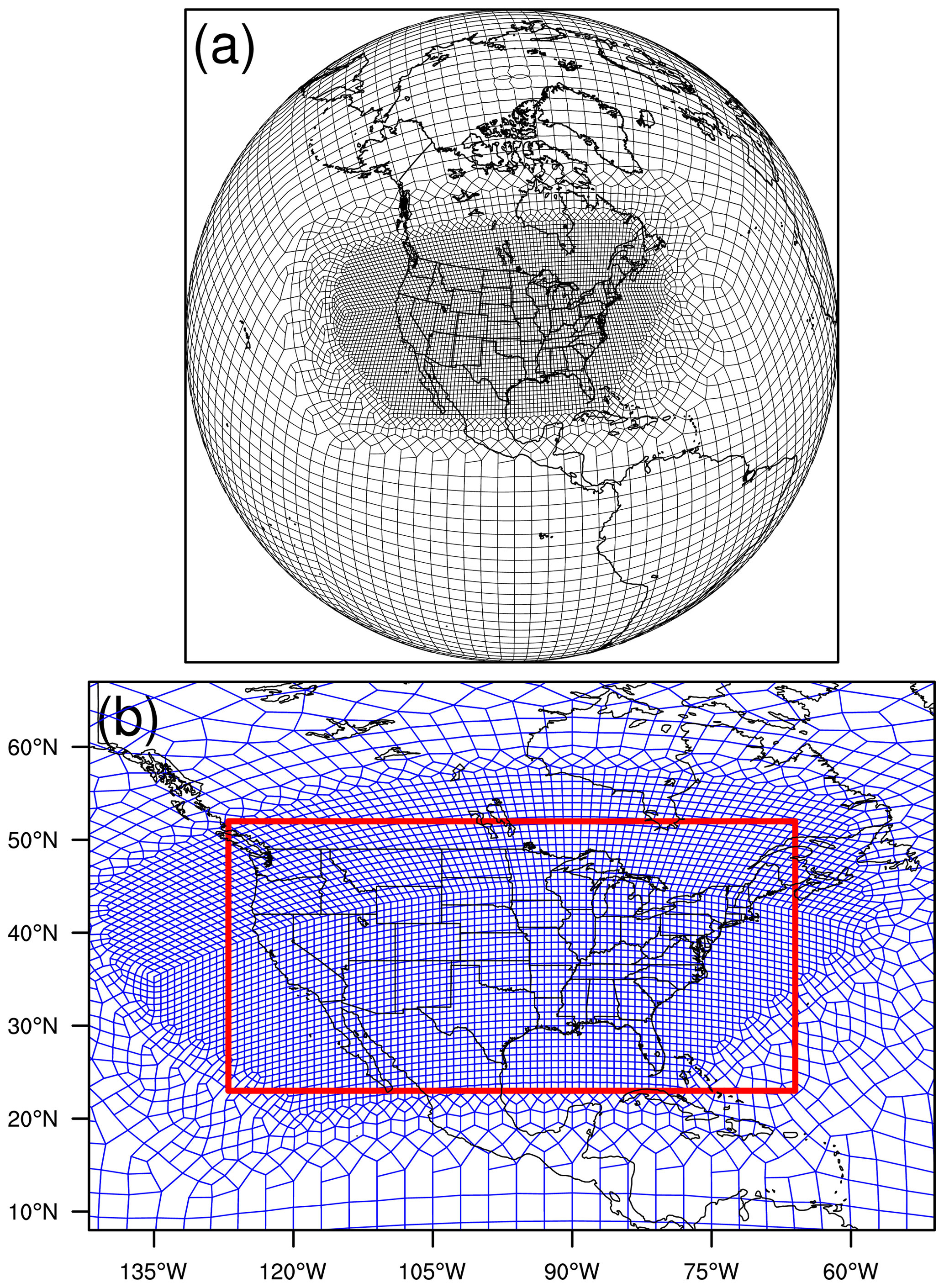
Figure 1E3SMv1 RRM domain (spectral elements) in (a) an orthographic projection and (b) a cylindrical equidistant projection. Panels (a) and (b) show the boundaries of spectral element grids. The red rectangle in panel (b) outlines the region we focus on in the following analyses, which is referred to as the RRM region.
The atmospheric and land initial conditions in the LR simulation are derived from an earlier E3SMv1 simulation, which has reached equilibrium. The RRM initial conditions are regridded from those of the LR simulation to exclude the potential impact of distinct initial conditions on the simulation results. Anthropogenic and biomass burning emissions of BC, POM, and SO4 and precursor gas sulfur dioxide (SO2) are from the CMIP6 emission inventory (Feng et al., 2020; Hoesly et al., 2018). Notably, we use the emission data in 2014 instead of in 2016 due to the data availability of CMIP6. Dimethyl sulfide (DMS) emissions in 1850, 2000, and 2100 are estimated from a coupled model simulation with a detailed representation of DMS formation in the seawater (Wang et al., 2018). We obtain the DMS emissions in 2014 through linear interpolation of the emissions in 1850, 2000, and 2100. The 3-D SOA production rates (implemented similarly to emissions) are derived from the simulation from Shrivastava et al. (2015). Besides the PD LR and RRM simulations, we run two corresponding simulations with PI aerosol emissions to calculate ERFaer. The PI simulation configurations are the same as the corresponding PD simulations, except that emissions of BC, POM, SO4, SO2, DMS, and SOA (production) in 1850 are used in the PI simulations.
We apply nudging globally in the LR and RRM simulations, which differs from Tang et al. (2019), which used nudging only on the low-resolution meshes but not the high-resolution grids in CONUS. We follow the nudging strategy from Zhang et al. (2014) and Sun et al. (2019), which demonstrated that a simulation with constraint horizontal winds could reproduce the evolution characteristics of the observed weather events and the model's long-term climatology. In addition, it has been corroborated that nudged simulations with a relatively short simulation period (e.g., 1 year) can reproduce the annual mean changes in aerosol burdens and optical depths caused by anthropogenic aerosols in the E3SM Atmospheric Model Intercomparison Project (AMIP) simulations (K. Zhang et al., 2022). The short nudged simulations also have a similar estimate of ERFaer as that of the AMIP-type free-running simulations (K. Zhang et al., 2022). Moreover, by constraining the large-scale circulation, nudging helps suppress the noise caused by the chaotic response to model changes and facilitates the comparison between the LR and RRM simulations. Similarly, nudging is also used to estimate ERFaer, as recommended by previous studies (Kooperman et al., 2012; Sun et al., 2019; Zhang et al., 2014). In short, nudging helps increase the signal-to-noise ratio and identify the impact caused by regional refinement more quickly. In our simulations, the horizontal winds are nudged toward the European Centre for Medium-Range Weather Forecasts Reanalysis v5 (ERA5) (Hersbach et al., 2020), with a relaxation time of 6 h (S. Zhang et al., 2022). To avoid the errors caused by vertical interpolation–extrapolation from ERA5 to E3SM vertical levels, we do not apply nudging for model levels below 950 hPa and above 10 hPa.
Several parameters differ between the E3SMv1 standard LR and CONUS RRM default configurations. For example, the time step for most physical processes and the coupling between physics and dynamics is 30 min in the LR configuration. In comparison, CONUS RRM uses a time step of 15 min. Many physical processes are sensitive to the time step and parameter setting (Wan et al., 2015, 2021; Zhao et al., 2013). Our sensitivity tests show substantial differences in the aerosol mass and energy budgets even outside of the refined region when the respective default configurations are used in the LR and RRM simulations, which is mainly attributed to their distinct physical time steps (not shown). Therefore, it would be better to keep the tuning parameters and time step the same between the LR and RRM simulations to isolate the regional refinement effect (horizontal resolution sensitivity), as recommended by earlier studies (Caldwell et al., 2021; Ma et al., 2015). Therefore, for the LR simulation, we use the time step of 15 min and the parameter setting from the default CONUS RRM configuration. With such changes, LR shares the same configuration as RRM, except for regional refinement around CONUS (Fig. 1) and resolution-relevant input files (e.g., topography and nudging-prescribed wind fields). As expected, the results are very close between the LR and RRM simulations in the low-resolution (∼ 100 km) areas (not shown), facilitating our subsequent investigation of the impacts of regional refinement on the aerosol mass budget and the aerosol forcing over CONUS.
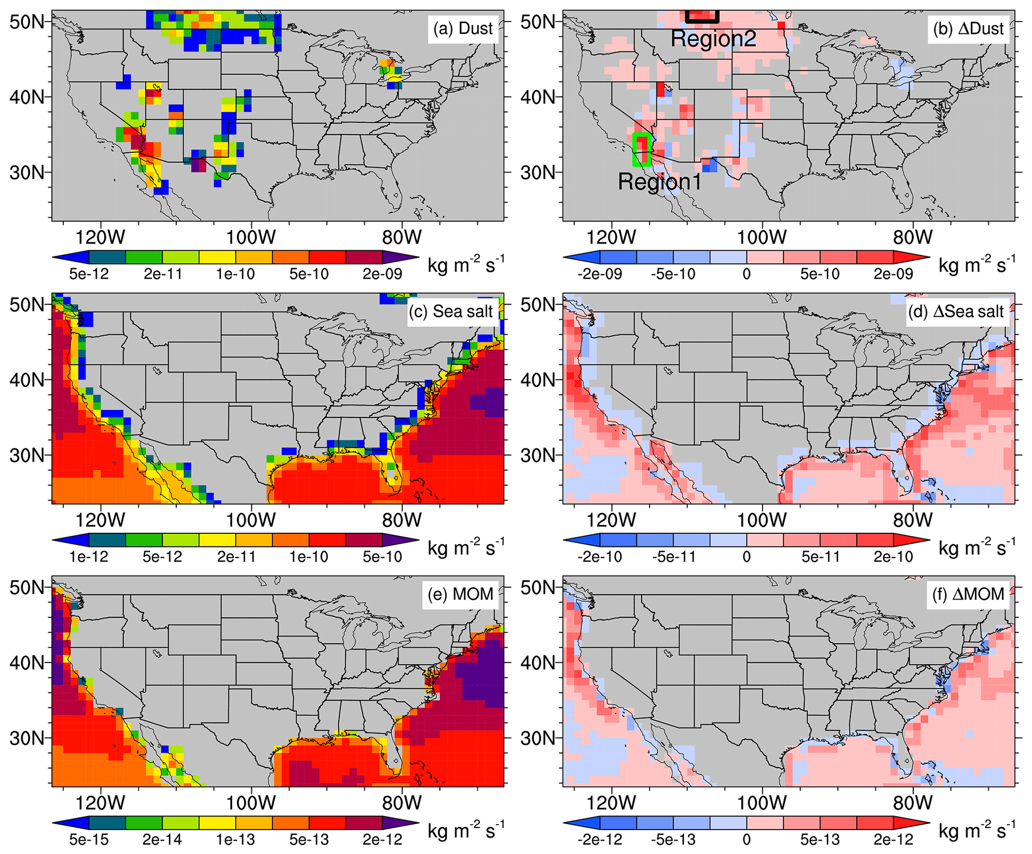
Figure 2(a, c, e) Spatial distributions of annual mean sources of (a) dust, (c) sea salt, and (e) MOM from the LR simulation. (b, d, f) The same as the left column but for the absolute differences between the RRM and LR simulations (RRM–LR). The green and black boxes in panel (b) highlight two subregions with substantial changes in dust emissions when applying regional refinement. Region 1 is around the Mohave and Sonoran deserts, and Region 2 is in the northern North American Prairie.
We focus our analysis on the refined region, as outlined by the red box in Fig. 1b (hereafter referred to as the RRM region), and the annual mean simulation results in 2016, unless stated otherwise. The LR and RRM simulation results have been regridded to 1∘ × 1∘ to facilitate their comparison, unless otherwise indicated.
3.1 Aerosol natural sources
Table 1 summarizes the annual mean sources and burdens of the seven aerosol species in the RRM region from the LR and RRM simulations. We find the largest relative differences in the sources and mass burden of the natural wind-driven aerosols between the RRM and LR simulations. With higher horizontal resolution, the RRM simulation produces more dust (154 %), sea salt (13 %), and MOM (10 %) emissions than LR. The dust emission enhancement by RRM is concentrated in several inland regions with high dust emissions, especially in the Mohave and Sonoran deserts (referred to as Region 1) and the northern North American Prairie (referred to as Region 2) (Fig. 2a and b). In comparison, the increases in sea salt and MOM emissions mainly occur around the coastal lines (Fig. 2c–f). That dust emissions increase with finer model resolutions has been identified in earlier studies (Caldwell et al., 2019; Feng et al., 2022; Ridley et al., 2013), which attributed the increase to more frequent occurrences of strong winds in high-resolution simulations. Dust emissions are nonlinearly correlated with surface winds and are particularly sensitive to strong winds (Zender et al., 2003). We find larger (11.2 %) annual mean surface wind speeds and more frequent strong winds in Region 1 in the RRM simulation compared to the LR simulation (Fig. 3c and d), which can explain the dust emission increase in Region 1 under regional refinement (Fig. 2b). However, in Region 2, the annual mean surface wind speeds differ slightly (2.2 %) between the RRM and LR simulations. Besides, the probability density functions (PDFs) of wind speed in Region 2 are similar between the two simulations (Fig. 3c and e), as well as the PDFs of friction velocity (not shown), indicating that surface winds and friction velocities alone cannot explain the dust emission enhancement in the RRM simulation. In addition to surface winds and friction velocity, soil moisture can also influence dust emissions by improving the friction velocity threshold (Namikas and Sherman, 1997; Zender et al., 2003). Therefore, high soil moisture may inhibit saltation and thus reduce dust emissions. We find lower (−7.1 %) volumetric soil water content in the surface layer in Region 2 in the RRM simulation than in the LR simulation (Fig. 3b), which is consistent with the dust emission increase in the region by RRM (Fig. 2b). The reduced surface soil water content in Region 2 is likely related to less precipitation (−3.0 %) in the RRM simulation compared to the LR simulation (Fig. 4c).
Table 1Total annual mean sources and burden in the RRM region for the seven aerosol species.
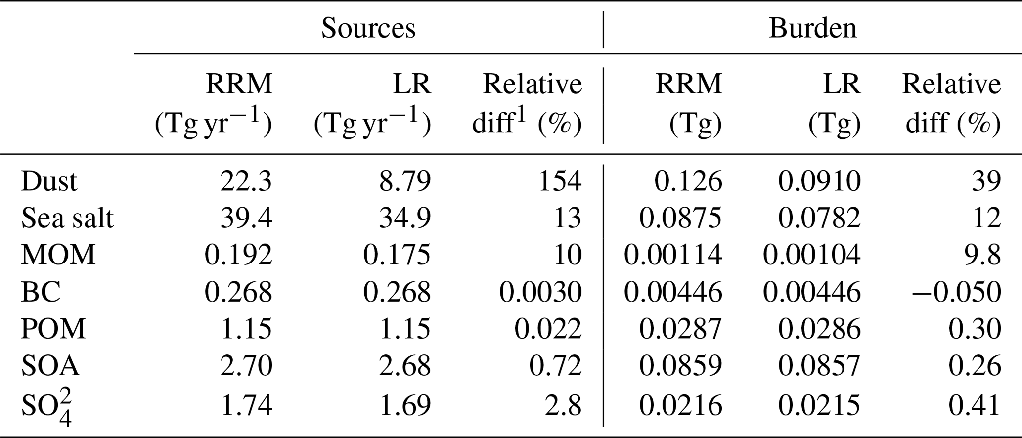
1 Relative diff is . 2 SO4 is represented in the mass of sulfur (TgS yr−1 for sources and TgS for burden). Besides direct anthropogenic emissions of SO4, other SO4 sources include gas–aerosol exchange, aqueous-phase production (aqueous-phase chemistry and cloud water uptake), and new particle formation.
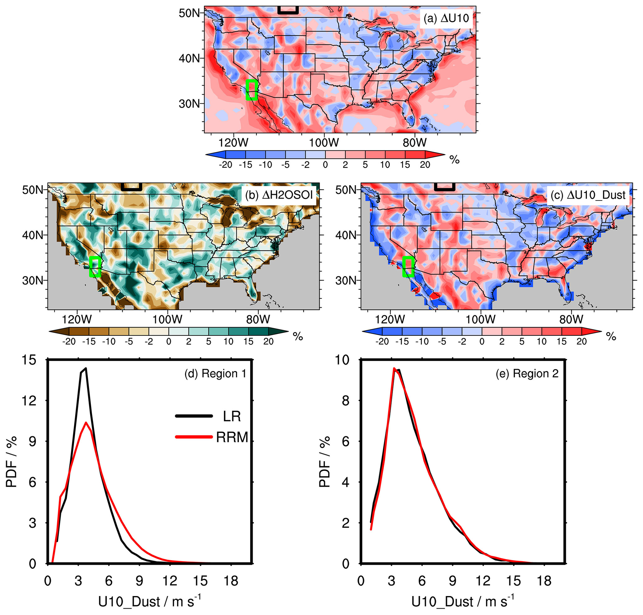
Figure 3Spatial distributions of the relative differences in annual mean (a) 10 m wind speed from the E3SMv1 atmospheric component (U10), (b) surface-layer volumetric soil water content (H2OSOI), and (c) 10 m wind speed used in the dust emission parameterization (U10_Dust) between the RRM and LR simulations (RRM-LR). The green and black boxes in panels (a), (b), and (c) are the same as those in Fig. 2b. (d, e) Probability density functions (PDFs) of U10_Dust in (d) Region 1 and (e) Region 2. The black lines are for the LR simulation, while the red lines are for the RRM simulation. U10_Dust on native model grids with an output frequency of 15 min is used to derive the corresponding PDF. Notably, U10_Dust is slightly different from U10, which considers the convective gustiness effect.
As mentioned above, sea salt and MOM emissions are related to surface wind speed and sea surface temperature (Burrows et al., 2022; Liu et al., 2012). We attribute the increased sea salt and MOM emissions in the RRM simulation to enhanced surface wind speeds at the finer model resolution, as shown in Fig. 3a. In addition, since sea salt and MOM are only emitted over the ocean, the distinct land–ocean boundaries may also partially contribute to the discrepancies in sea salt and MOM emissions between the RRM and LR simulations.
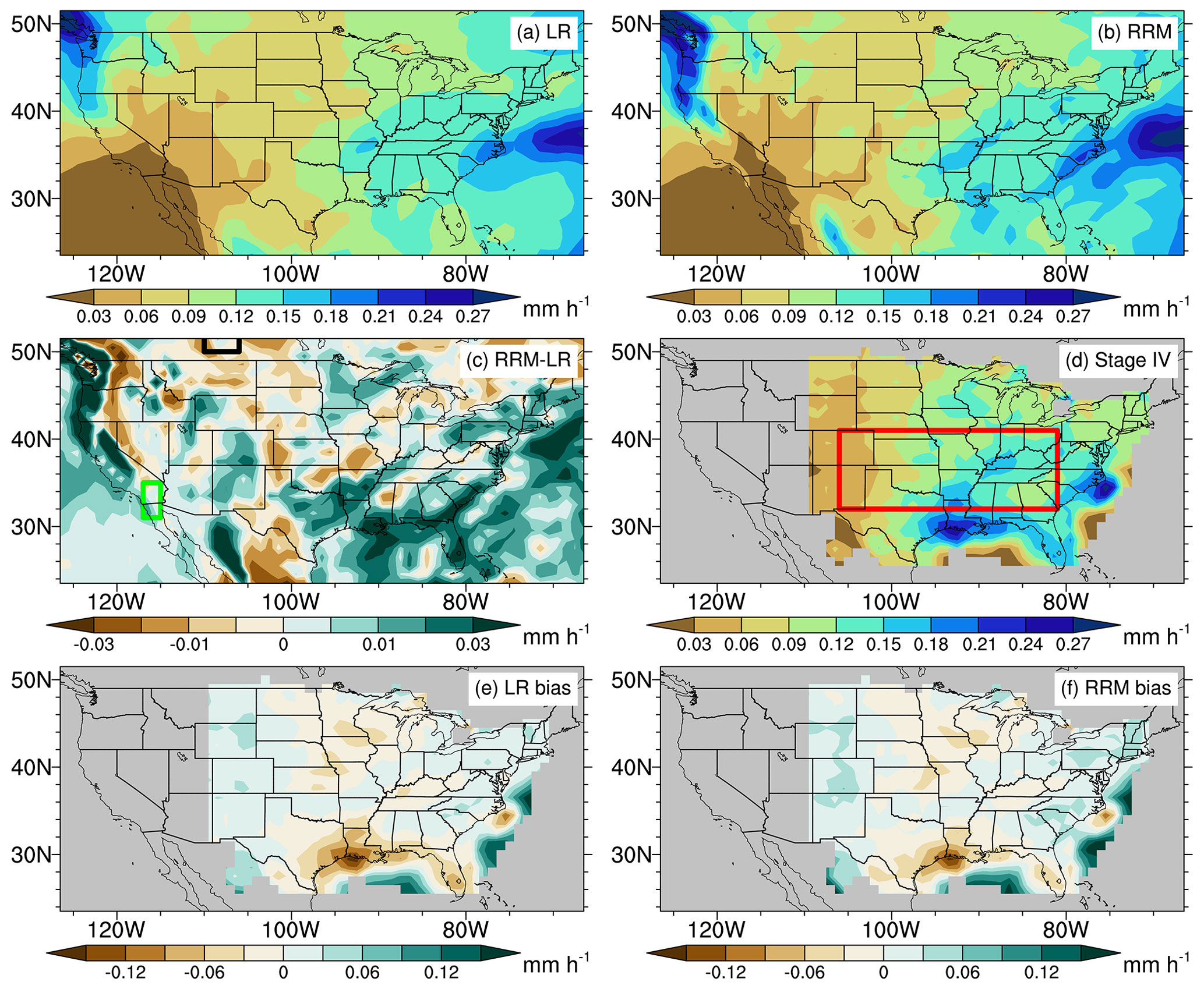
Figure 4(a–c) Spatial distributions of annual mean total precipitation rates (large scale and convective) for the (a) LR and (b) RRM simulations and (c) their differences (RRM–LR). The green and black boxes in panel (c) are the same as those in Fig. 2b. (d–f) Spatial distributions of annual mean precipitation from Stage IV and the precipitation bias of the LR and RRM simulations compared to Stage IV. The regional mean biases of the LR and RRM simulations are 0.004 and 0.010 mm h−1 compared to Stage IV, with a regional mean precipitation of 0.107 mm h−1. It is noteworthy that the data quality of Stage IV is poor over the open ocean and the western United States due to limited radar coverage. The Hovmöller diagram in Fig. 5 is based on the red box in panel (d).
3.2 Aerosol wet scavenging by convective vs. large-scale precipitation
In the RRM region, wet scavenging is the primary sink for most aerosol species in both simulations, except for dust and sea salt, the sinks of which are dominated by dry deposition. To understand the impact of horizontal grid spacing on aerosol wet scavenging, it is necessary first to investigate how precipitation differs between the LR and RRM simulations.
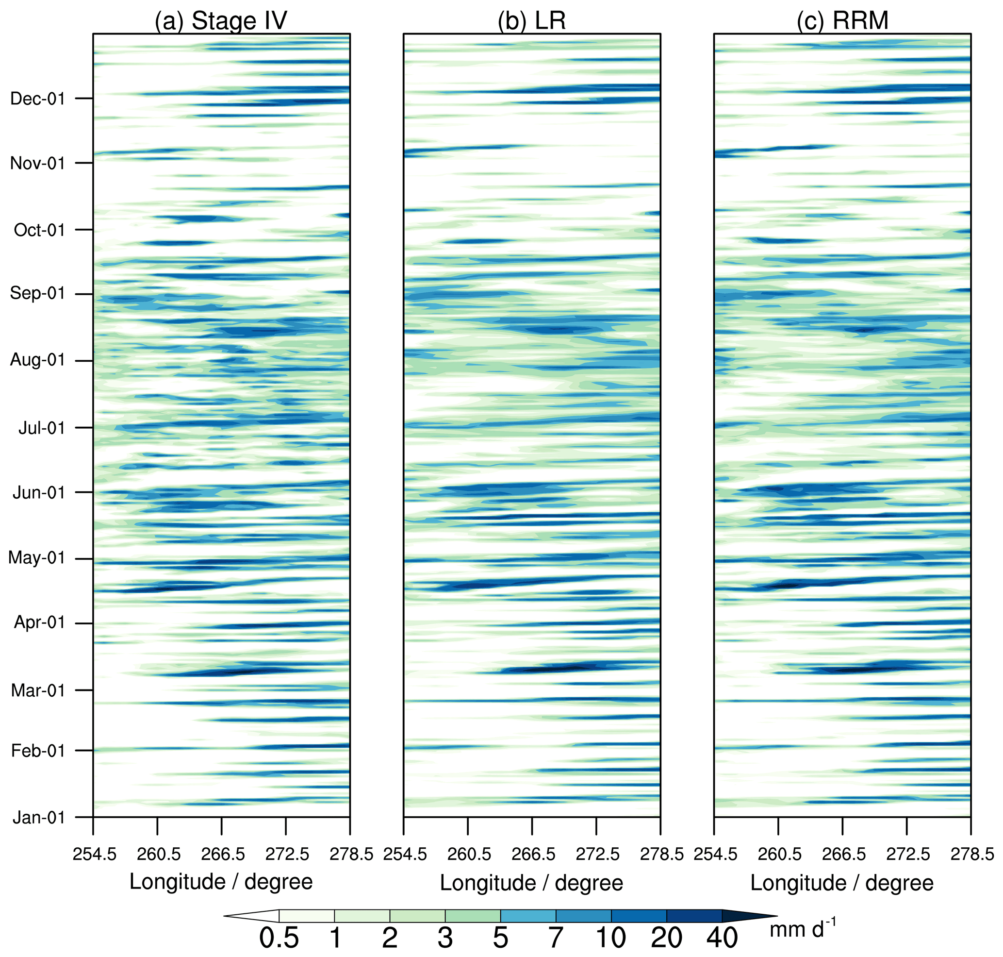
Figure 5Hovmöller diagrams of meridionally averaged daily precipitation rates in the red box of Fig. 4d for (a) Stage IV, (b) the LR simulation, and (c) the RRM simulation in 2016. The centered pattern correlation coefficient between LR and Stage IV is 0.28 (the same as that between RRM and Stage IV). The root mean square errors of LR and RRM are 5.3 and 5.5 mm d−1, respectively, compared to Stage IV.
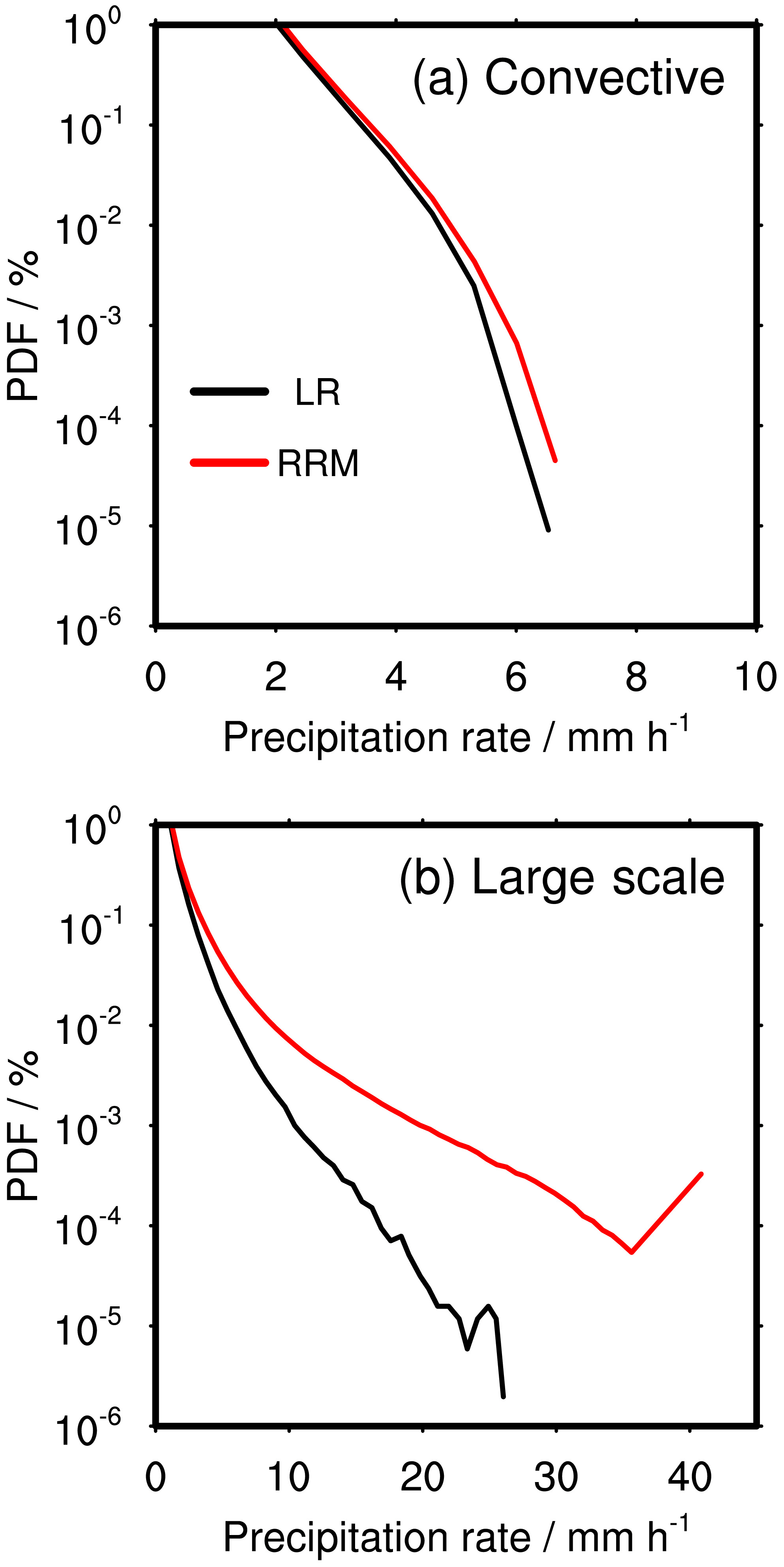
Figure 6Probability density functions (PDFs) of (a) convective and (b) large-scale precipitation rates in the RRM region for the LR (black lines) and RRM (red lines) simulations. Precipitation on native grids with an output frequency of 15 min is used to calculate the corresponding PDF.
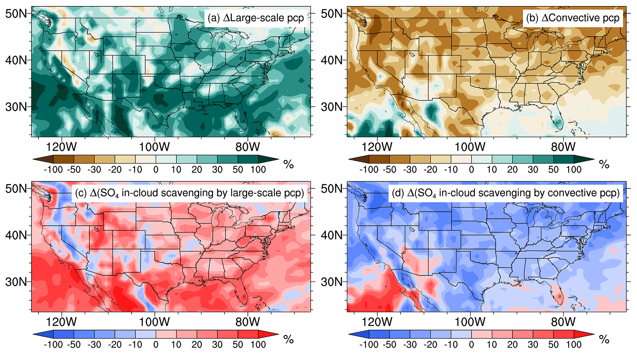
Figure 7(a, b) Spatial distributions of the relative differences in annual mean (a) large-scale and (b) convective precipitation between the RRM and LR simulations. (c, d) Same as panels (a) and (b) but for in-cloud scavenging of SO4 by (c) large-scale and (d) convective precipitation.
Figure 4 evaluates the LR and RRM simulated precipitation against the observational Stage IV data. Stage IV is a radar-based precipitation product with rain-gauge bias adjustment and has a native resolution of 4 km (Lin and Mitchell, 2005). We regrid the Stage IV data to 1∘ × 1∘ for comparison with our simulation results. Both simulations can capture the observed east–west precipitation gradient in the United States east of the Rocky Mountains. The spatial correlation coefficient between the LR simulation and Stage IV is 0.52, similar to that between RRM and Stage IV. Moreover, most observed precipitation events in the central–eastern United States (red box in Fig. 4d) are well simulated by the LR and RRM simulations, according to the Hovmöller diagrams of meridionally averaged daily precipitation rates in Fig. 5, which is attributed to the appropriate nudging strategy applied to the simulations. However, apparent dry biases are found near the coastal areas of the southern United States in the LR simulation (Fig. 4e). By producing more precipitation than the LR simulation around the United States coastal areas, RRM can reduce the dry bias in the southern coastal regions. However, its precipitation is still much lower than observed (Fig. 4f). Minor dry biases are also found in the northern Great Plains in both simulations. The model dry biases in the southern and northern Great Plains may be due to the limitation of E3SM in predicting extreme precipitation events, such as mesoscale convective systems (Feng et al., 2021; Wang et al., 2021), which is the dominant precipitation contributor in the Great Plains (Li et al., 2021). A noticeable improvement in the RRM simulation compared to the LR simulation is the production of more frequent heavy precipitation (> 7.6 mm h−1), which is mainly attributed to the intensification of large-scale precipitation (Fig. 6), consistent with the results from Caldwell et al. (2019). More frequent heavy precipitation can partially alleviate the “too frequent, too weak” problem in low-resolution E3SM simulations (Caldwell et al., 2019). However, our result contradicts that of Tang et al. (2019), which found more light precipitation but less heavy precipitation as the model horizontal resolution increases. It may be because Tang et al. (2019) did not apply nudging to their low-resolution and RRM simulations, and precipitation varied a great deal between the two simulations.
In addition to affecting total precipitation rates, the model resolution notably changes the partitioning between large-scale precipitation (that is computed by the MG2 cloud microphysics parameterization) and deep convective precipitation (that is computed by the ZM deep convection parameterization). As the model resolution increases, more precipitation can be resolved, which leads to an increase in large-scale precipitation and a decrease in convective precipitation (Fig. 7a and b) (Tang et al., 2019).
In E3SMv1, aerosol wet removal by large-scale and convective precipitation is comprised of in-cloud scavenging, which involves the activation of interstitial aerosol particles (IAPs) and the subsequent removal of cloud-borne aerosol by precipitation, and below-cloud scavenging accounting for the removal of IAPs by precipitation via impaction and Brownian diffusion (Liu et al., 2012; Wang et al., 2013). In-cloud scavenging is the dominant process for all aerosol species in the RRM region, accounting for ∼ 80 % of the wet removal of sea salt and dust and more than 98 % of the other aerosol species.
EAMv1 uses two different parameterizations to treat aerosol wet scavenging by large-scale clouds and deep convective clouds. Here, “large-scale clouds” refer to clouds represented by the CLUBB and MG2 parameterizations, and “deep convective clouds” refer to clouds represented by the ZM deep convection parameterization. In large-scale clouds, aerosol activation is parameterized as a function of subgrid vertical velocity (Wsub), aerosol properties, and environmental conditions (Abdul-Razzak and Ghan, 2000). The first-order loss rates of aerosol are computed by multiplying a solubility factor by the first-order loss rate of cloud water, which is computed as a function of cloud fraction, cloud water, and precipitation production rate profiles (Barth et al., 2000; Rasch et al., 2000). In deep convective clouds, the cloud-borne aerosol mixing ratios are computed by multiplying interstitial aerosol mixing ratios by the prescribed convective-cloud activation fractions, which depend on aerosol modes and species to represent the hygroscopicity (Liu et al., 2012; Wang et al., 2013). The solubility factor is a tunable parameter, and the model uses different solubility factors for large-scale and deep convective clouds (Liu et al., 2012; Wang et al., 2013).
Therefore, the change in the partitioning between large-scale and deep convective precipitation should make a difference in aerosol wet removal. Taking SO4 as an example, Fig. 7c and d show a significant increase in in-cloud scavenging of SO4 by large-scale precipitation but a noticeable decrease by deep convective precipitation in the RRM simulation compared to the LR simulation. The changing patterns of in-cloud scavenging by large-scale and deep convective precipitation are consistent with the changes in the corresponding type of precipitation rates. Figure 8 summarizes the relative differences in regional mean large-scale and deep convective in-cloud scavenging of different aerosol species in the RRM region between the RRM and LR simulations. Due to the increase in large-scale precipitation (28 %) and the decrease in deep convective precipitation (−16 %) in the RRM region, the large-scale in-cloud scavenging increases, and the deep convective in-cloud scavenging reduces for all aerosol species, except for dust in the RRM simulation compared to the LR simulation. Dust exhibits a different response because the dust emission is 154 % higher in the RRM simulation than in the LR simulation. With the significant increase in the dust emission and loading in the atmosphere in the RRM simulation, the wet removal of dust by both large-scale and deep convective clouds is higher than that in the LR simulation, even though the deep convective precipitation rate is lower.
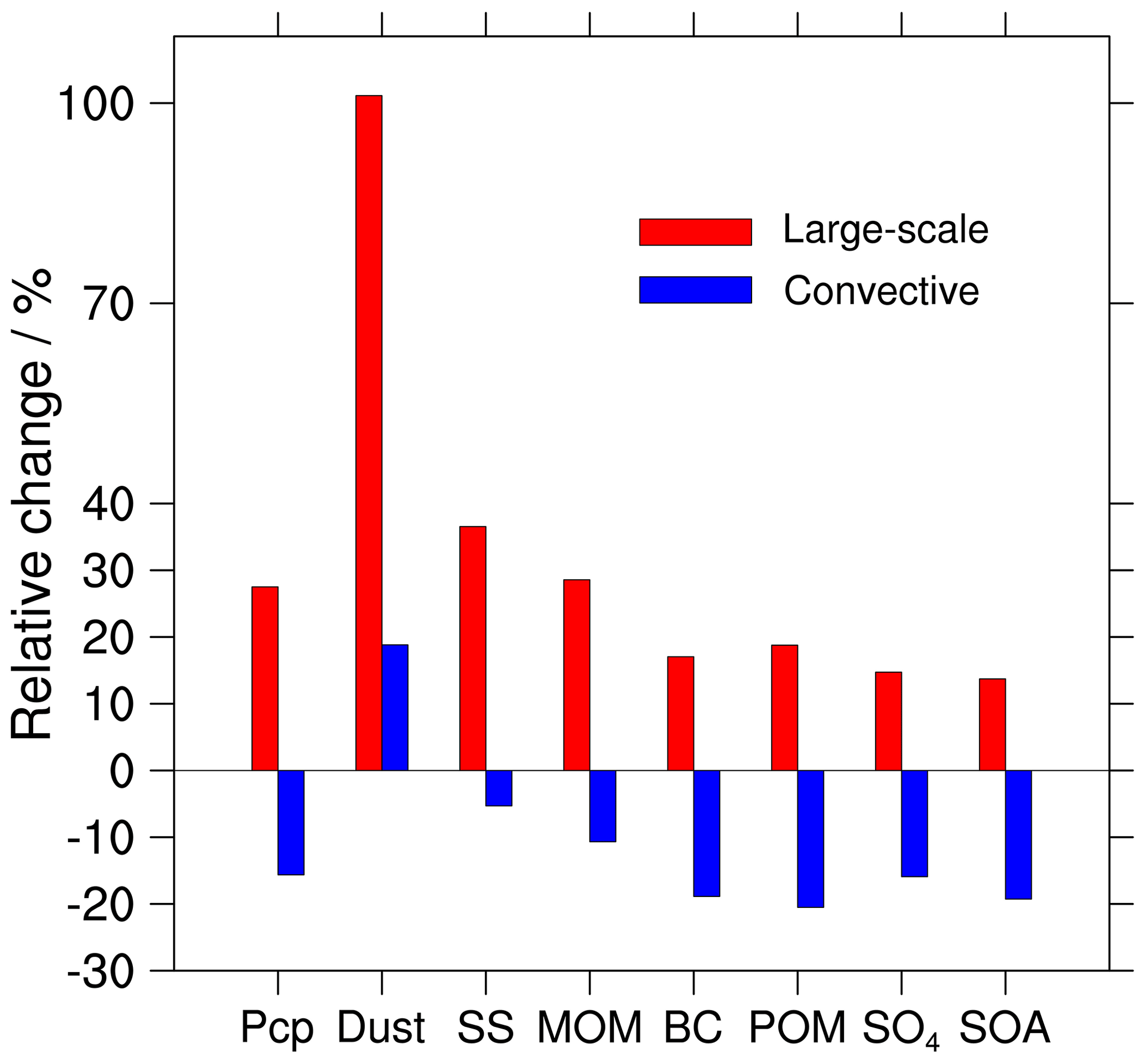
Figure 8Relative differences in annual regional mean large-scale and convective precipitation and in-cloud scavenging of different aerosol species by large-scale and convective precipitation between the RRM and LR simulations. Pcp refers to precipitation, and SS denotes sea salt.
3.3 Aerosol chemical production
As expected, anthropogenic aerosol emissions (e.g., BC, POM, and SOA) prescribed by offline emission inventories are almost the same between the RRM and LR simulations. However, the SO4 source in the RRM simulation is 2.8 % higher (Table 1). MAM4 considers four source terms for sulfate aerosol. Two primary sources of SO4 are gas–aerosol exchange and aqueous-phase production (Fig. S3), which contribute to 31 % and 63 %, respectively, in the RRM region. The other two minor source terms are (1) direct emission of sulfate aerosol and (2) new particle formation (NPF) (Fig. S3), accounting for about 5 % and 1 % of the total source. Figure 9a and c show the spatial distributions of SO4 production via the two major pathways from the LR simulation, generally consistent with the distributions of precursor gases (sulfuric acid gas vapor (H2SO4) and SO2 in Fig. S4a and b), with one peak in the northeastern United States and another peak around southwestern Texas. The RRM simulation generally produces more SO4 via aqueous-phase production (6.2 % on average over the RRM region) but less via gas–aerosol exchange (−3.0 %) than the LR simulation (Fig. 9b and d). Figure 9e–f show that increasing resolution leads to significantly lower (−13.3 %) NPF of SO4.
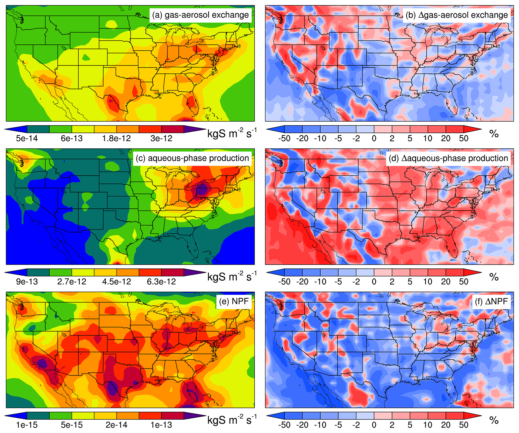
Figure 9(a, c, e) Spatial distributions of annual mean SO4 sources from (a) gas–aerosol exchange, (c) aqueous-phase production, and (e) NPF in the LR simulation. (b, d, f) The same as the left column but for the relative differences between the RRM and LR simulations.
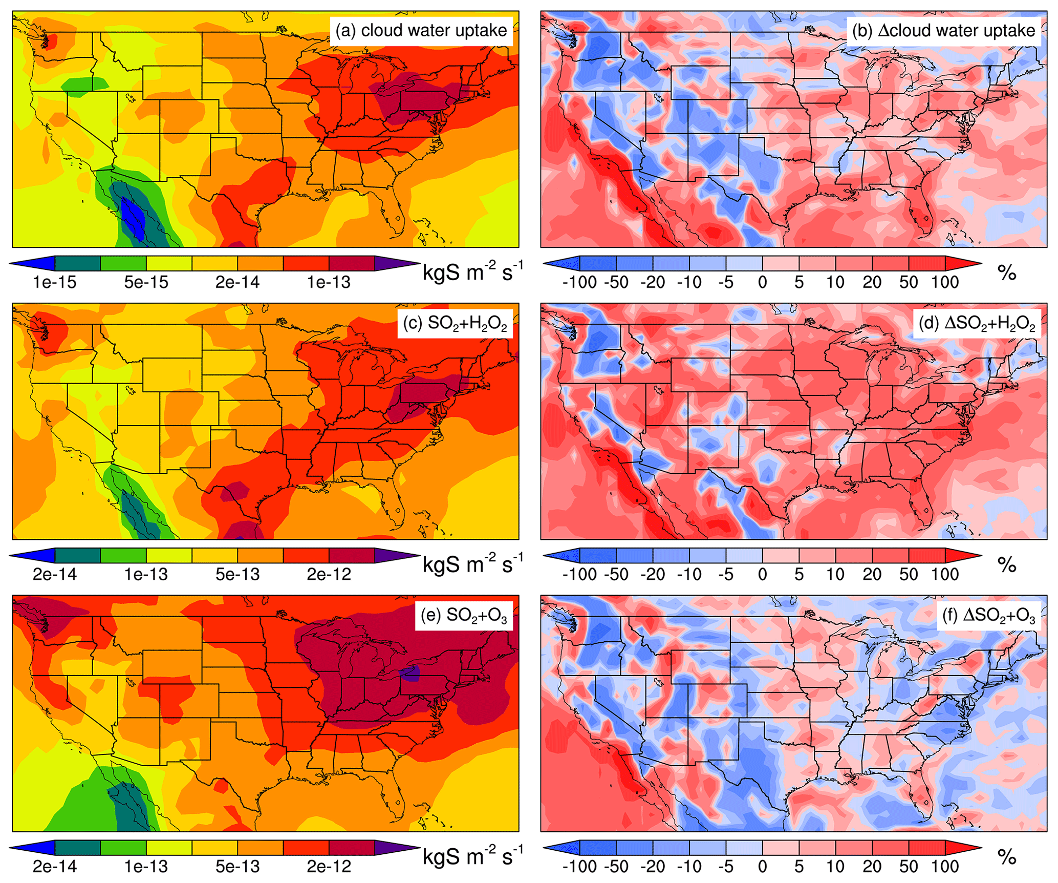
Figure 10(a, c, e) Spatial distributions of annual mean SO4 aqueous-phase productions through (a) cloud water uptake, (c) the H2O2 oxidation pathway, and (e) the O3 oxidation pathway in the LR simulation. (b, d, f) The same as the left column but for the relative differences between the RRM and LR simulations. It is noteworthy that the aqueous-phase production occurs in large-scale clouds.
SO4 production via gas–aerosol exchange and NPF positively correlates with the H2SO4 concentration (Liu et al., 2012). We find a lower (−5.5 %) H2SO4 concentration in the RRM than in the LR (Fig. S5a), which can explain the reduction in the SO4 production via gas–aerosol exchange and NPF (Fig. S3). The source of H2SO4 is the oxidation of gas-phase SO2 by hydroxyl radical (OH) (Fig. S3). In our E3SMv1 configuration, OH concentrations are prescribed, and the reaction rate constants of SO2 and OH are similar between the RRM and LR simulations (not shown). Therefore, the H2SO4 production is dominated by the gas-phase SO2 concentration, which shows a reduction (−2.3 %) in the RRM compared to the LR (Fig. S5b). The sources of gas-phase SO2 include direct emissions and the oxidation of DMS by OH and nitrate radical (NO3) (Fig. S3). DMS and SO2 emissions are read from emission inventories, and the reaction rate constants of DMS + OH and DMS + NO3 are close between the RRM and LR simulations. Therefore, the gas-phase SO2 source is similar between the two simulations, and we need to understand the sinks of gas-phase SO2 to explain the general reduction in the gas-phase SO2 concentrations in the RRM simulation. We find that dry and wet deposition cannot explain the general reduction in the gas-phase SO2 concentrations in the RRM compared to the LR (not shown). Another major sink of gas-phase SO2 is the oxidation of SO2 by hydrogen peroxide (H2O2) and ozone (O3) to form SO4 via aqueous-phase chemistry (Figs. 10c, e, and S3). Another process to produce SO4 in the aqueous-phase chemistry module of E3SMv1 is the cloud water uptake of H2SO4 (Figs. 10a and S3). All three pathways are related to large-scale cloud liquid water content (LWC) (LWC at 700 hPa shown in Fig. S4c). The RRM simulation generally produces a larger LWC than the LR simulation (700 hPa, shown as an example in Fig. S5c). Therefore, the cloud water uptake of H2SO4 is enhanced in the RRM simulation (Figs. 10b and S3).
The aqueous-phase oxidation of SO2 by H2O2 and O3 would also be expected to increase with higher LWC in the RRM simulation. However, we find a slight reduction (−1.2 %) in SO4 production via the O3 pathway (Fig. 10f). In contrast, the H2O2 pathway is enhanced by 17.0 % in the RRM simulation compared to the LR simulation (Fig. 10d).
The H2O2 and O3 pathways differ in two aspects. First, the O3 concentrations are prescribed, while the H2O2 concentrations are prognostic in our E3SMv1 configuration (Figs. S3 and S4e). Second, the O3 pathway is highly sensitive to the pH of the cloud water (proton (H+) concentrations at 700 hPa shown in Fig. S4d), while the H2O2 pathway is hardly affected by pH (Seinfeld and Pandis, 2016). We find that the gas-phase H2O2 concentrations are generally slightly higher in the RRM than the LR (Fig. S5e), even though the improved H2O2 pathway should consume more H2O2 under regional refinement. The budget analysis (not shown) indicates that the reduction in the gas-phase H2O2 wet removal in the RRM simulation contributes to the slightly enhanced H2O2 concentrations (Figs. S3, S4f, and S5f). The reduced wet removal is related to decreased net rain production (mainly convective) used in the wet deposition parameterization of gas species (not shown). Notably, the oxidation of SO2 by H2O2 releases H+ into cloud water (Fig. S3). With increased H2O2 concentrations, we expect higher H+ concentrations ([H+]) in large-scale clouds in the RRM simulation than in the LR simulation, as shown in Fig. S5d. Slightly higher [H+] (lower pH) would suppress the aqueous-phase oxidation of SO2 by O3 significantly (Seinfeld and Pandis, 2016). These results explain why the O3 pathway is suppressed slightly, even though LWC increases in the RRM simulation compared to the LR simulation.
In short (Fig. S3), higher LWC leads to more SO4 production via cloud water uptake and the aqueous-phase oxidation of SO2 by H2O2. However, the oxidation of SO2 by O3 is slightly suppressed due to the combination of larger LWC and lower pH. Finally, the total aqueous-phase SO4 production is enhanced in the RRM, which consumes more SO2 and leads to lower gas-phase SO2 concentrations compared to the LR.
3.4 Aerosol–cloud interactions
Aerosol activation in large-scale clouds is parameterized consistently with droplet nucleation. In EAMv1, most IAPs exist in accumulation and Aitken modes (Fig. S6a and b). We find the aerosol activation in the RRM is, on average, enhanced by 13.7 % (accumulation mode) and 5.8 % (Aitken mode) compared to the LR (Fig. 11a and b). Aerosol activation in large-scale clouds primarily occurs in two pathways. One is related to cloud expansion (i.e., increase in cloud fraction, which leads to aerosol activation) and shrinkage (i.e., decrease in cloud fraction, which leads to aerosol resuspension) in the same grid box (hereafter referred to as the cloud-intermittency pathway) between model time steps. The other refers to the activation of IAPs that are brought to the cloud base by updrafts (hereafter referred to as the updraft pathway) (Liu et al., 2012). We find that the cloud-intermittency pathway contributes to almost all the aerosol activation enhancement in Aitken mode but only about half of the enhancement in accumulation mode under regional refinement (not shown). The updraft pathway accounts for the other half of the enhancement in accumulation mode. The contrast RRM impacts on the updraft pathway between the accumulation and Aitken modes may be related to the distinct vertical profiles of IAPs from the two modes (Fig. S6c). The cloud-intermittency pathway is parameterized as a function of Wsub, aerosol properties, and the change in large-scale liquid cloud fractions between two consecutive time steps (ΔLCLOUD) (Abdul-Razzak and Ghan, 2000; K. Zhang et al., 2022). Positive ΔLCLOUD corresponds to cloud expansion, and negative ΔLCLOUD denotes cloud shrinkage. We do not find any noticeable differences in Wsub and aerosol properties between the RRM and LR simulations. However, |ΔLCLOUD| is considerably larger in the RRM, which indicates larger LCLOUD temporal variability (Fig. 11c), resulting in increased microphysical cloud processing of aerosols and more aerosol activation via the cloud-intermittency pathway. The larger LCLOUD temporal variability is consistent with the larger relative humidity (RH) temporal variability in the RRM than in the LR (Fig. 11d) (Golaz et al., 2002).
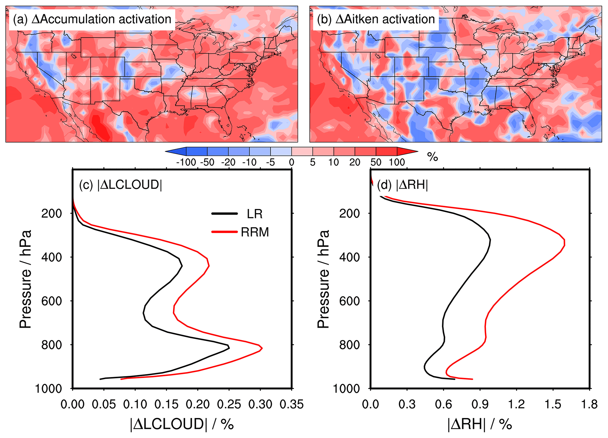
Figure 11(a, b) Spatial distributions of the relative differences in the annual mean vertical-integrated IAP activation fluxes in large-scale clouds for (a) accumulation and (b) Aitken modes between the RRM and LR simulations. (c) Vertical profiles of the annual regional mean absolute temporal variabilities in the large-scale liquid cloud fractions (|ΔLCLOUD|). ; t2 and t1 indicate two consecutive model time steps. The red line indicates the RRM simulation, and the black line is for the LR simulation. (d) The same as panel (c) but for relative humidity (RH).
Enhanced aerosol activation results in higher droplet number concentrations (Nd) in the RRM compared to the LR (Fig. 12a). Moreover, the CLUBB vertical-integrated cloud liquid water tendency (RCMTEND), which is dominated by water vapor condensation, is generally remarkably larger in the RRM simulation (Fig. 12b), which leads to higher large-scale cloud liquid water path (LWP) and LWC (Figs. 12c and S5c). Larger RCMTEND may also contribute to larger droplets at the cloud top in the RRM simulation (Re in Fig. 12d; Re – grid cell mean droplet effective radius at the top of liquid water clouds), even though Nd increases. With higher LWP and larger Re, cloud optical depth (COD) is also higher (Fig. 12e).
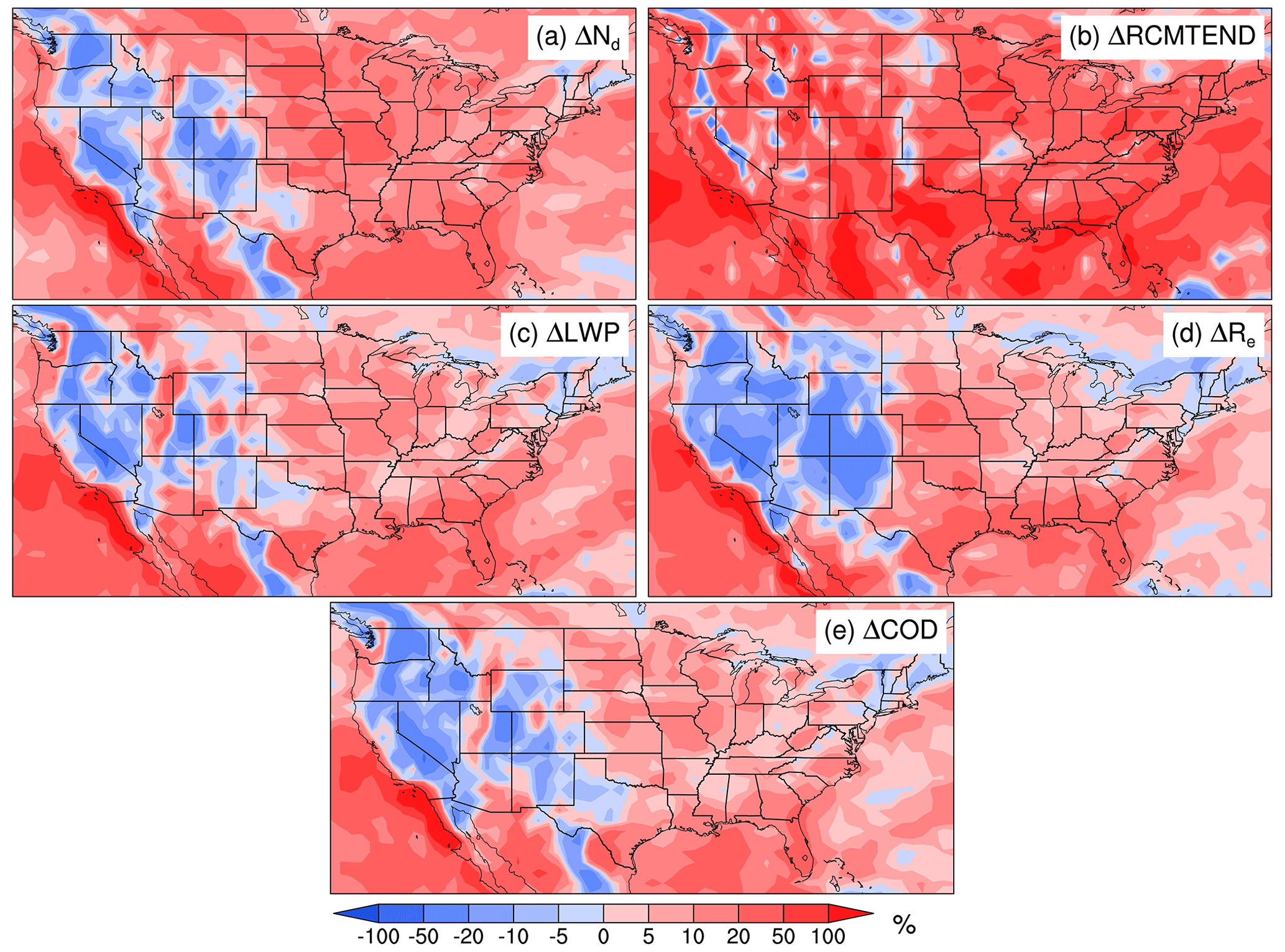
Figure 12Spatial distributions of the relative differences in annual mean (a) grid cell mean vertical-integrated droplet number concentrations (Nd), (b) CLUBB vertical-integrated cloud liquid water tendency (RCMTEND), (c) grid cell mean liquid water path (LWP), (d) grid cell mean droplet effective radius at the top of liquid water clouds (Re), and (e) grid cell mean cloud optical path (COD) between the RRM and LR simulations. It is noteworthy that Nd, RCMTEND, LWP, and Re are exclusively for large-scale clouds, while COD considers both large-scale and convective clouds but is dominated by large-scale clouds (not shown). The spatial distributions of Nd, RCMTEND, LWP, Re, and COD from the LR simulation are shown in Fig. S7.
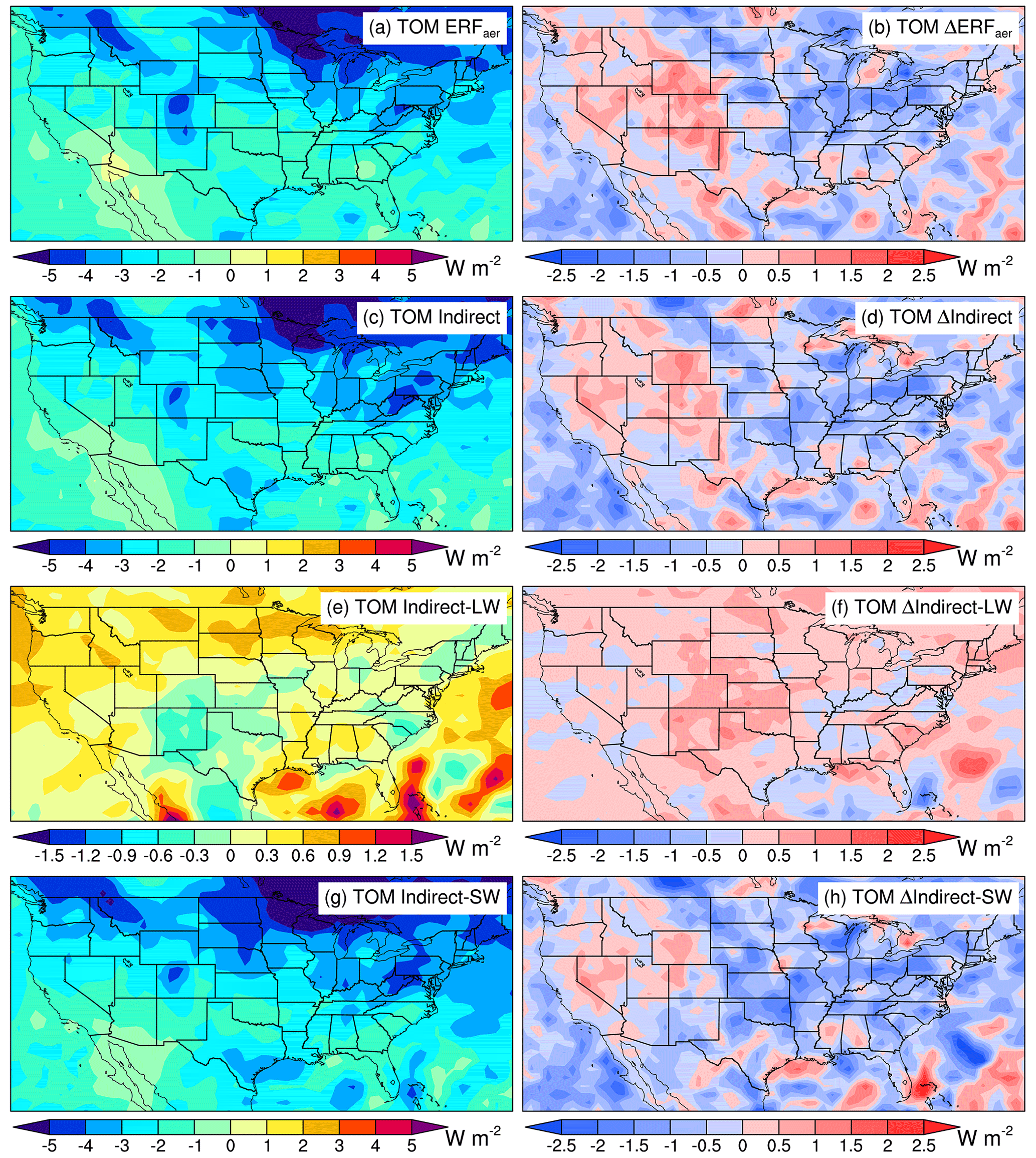
Figure 13(a) Spatial distribution of annual mean ERFaer at the top of the model (TOM) from the LR simulation. (c, e, g) Same as panel (a) but for ERFaer attributed to (c) aerosol indirect effect (longwave plus shortwave), (e) aerosol longwave indirect effect, and (g) aerosol shortwave indirect effect. The right column is the same as the left but for the absolute differences between the RRM and LR simulations.
3.5 Anthropogenic aerosol effective radiative forcing
With considerable impacts on cloud properties, the regional refinement should also influence ERFaer. We use the Ghan (2013) method to decompose ERFaer into direct, indirect, and surface albedo effects. Figure 13 shows a stronger (more negative) anthropogenic aerosol shortwave indirect effect (−0.52 W m−2) and enhanced longwave indirect effect (0.21 W m−2) at the top of the model (TOM) in the RRM simulation compared to the LR simulation. The net (shortwave plus longwave) indirect effect is 0.31 W m−2 more negative in the RRM simulation compared to the LR simulation, which is about a 12 % enhancement. The total ERFaer at TOM is 0.27 W m−2 more negative in the RRM simulation, about a 12 % enhancement compared to the LR simulation. We also find that the RRM simulation produces a 10 % enhancement of ERFaer at the surface (Fig. S8).
To understand the enhancement of ERFaer in the RRM experiment, we compare the production efficiencies of Nd, Re, LWP, and COD due to anthropogenic aerosols between the RRM and LR simulations (Fig. 14). In Fig. 14, the relative changes in Nd, LWP, and COD per relative change in CCN at 0.1 % supersaturation (CCN0.1 %) between the PD and PI simulations are generally larger in the RRM simulation, consistent with our earlier analysis of the enhanced aerosol activation in RRM. Because cloud properties are more sensitive to anthropogenic aerosols in the RRM, the RRM configuration produces stronger anthropogenic aerosol–cloud interactions and ERFaer (Fig. 13).
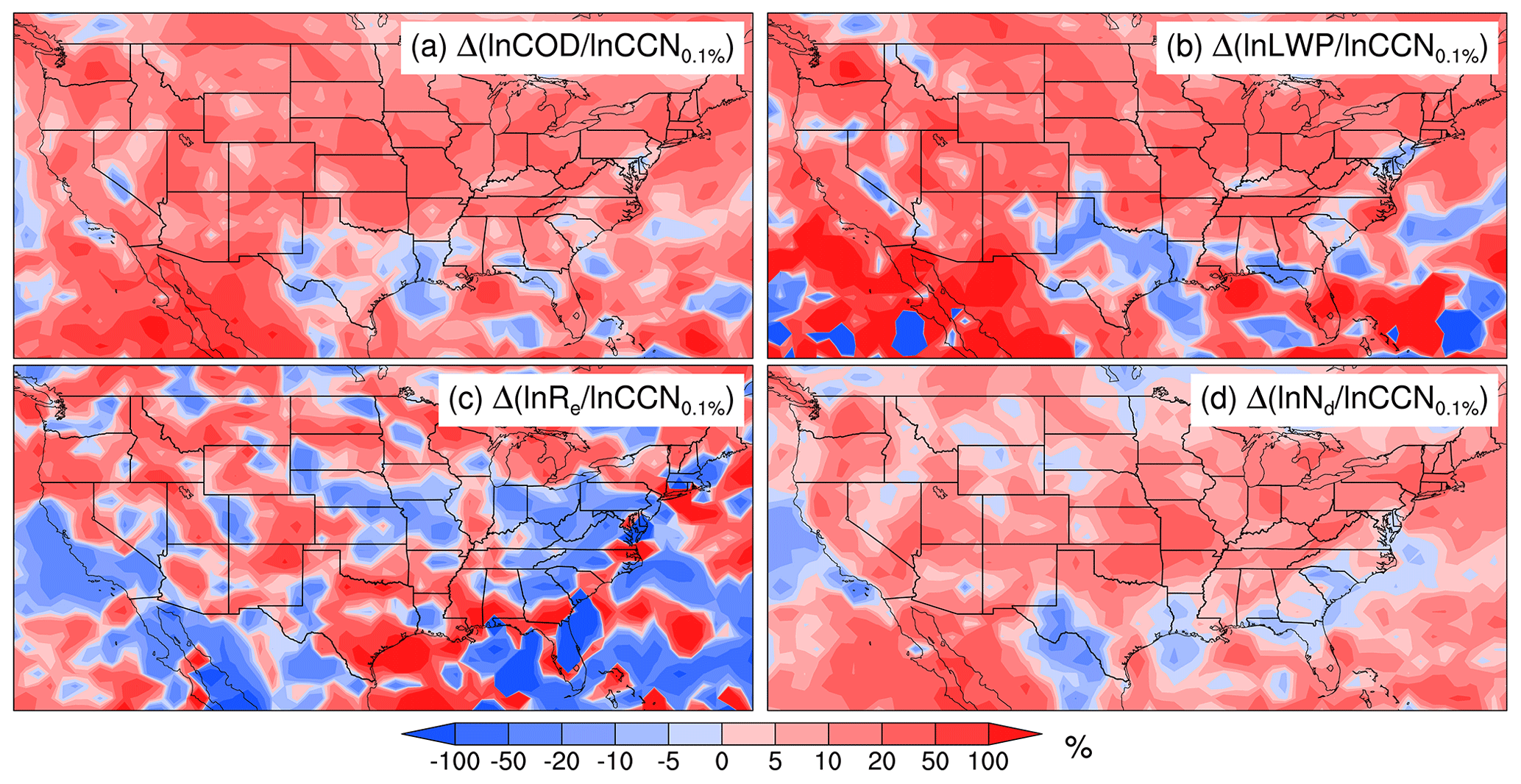
Figure 14Spatial distributions of the relative differences in (a) , (b) , (c) , and (d) between the RRM and LR simulations. Here, ln x denotes the relative change in x between the PD and PI simulations; i.e., . Therefore, reflects the production efficiency of x by anthropogenic aerosols.
This result differs from Ma et al. (2015), which demonstrated that higher model resolutions would weaken the aerosol indirect effect. Ma et al. (2015) identified the increased droplet nucleation in simulations with higher resolutions, leading to a stronger first aerosol indirect effect, which is consistent with this study. However, their LWP response to anthropogenic aerosols weakens (lower LWP) as resolution increases, leading to reduced second aerosol indirect effect, which is in contrast to the larger LWP production efficiencies in our RRM simulation (Fig. 14b). The discrepancies may be caused by different parameterizations of water vapor condensation to form cloud liquid water. The water vapor condensation is parameterized in CLUBB on the basis of joint PDFs of vertical velocity, temperature, and moisture in our simulations (Golaz et al., 2002), while it was calculated in CAM5 in Ma et al. (2015) using a saturation equilibrium adjustment approach (Park et al., 2014). The water vapor condensation parameterization affects not only LWP but also the subsequent aqueous-phase chemistry calculation discussed in Sect. 3.3. Therefore, it is necessary to evaluate the sensitivity of water vapor condensation to model resolutions when different parameterizations are used, as their resolution sensitivity can be very different.
Our finding regarding the stronger aerosol indirect effect as resolution increases is also different from Caldwell et al. (2019), who found that the aerosol indirect effect changed only slightly from the low-resolution to high-resolution simulations. This discrepancy might be attributed to the fact that the model time steps used in low- and high-resolution model simulations are very different in Caldwell et al. (2019) but are kept the same in this study. Since the model time step can affect model aerosol and clouds, aerosol indirect effects can be affected.
We investigate the impact of increasing model horizontal resolution on the aerosol mass budget and ERFaer over the CONUS in 2016 by comparing E3SMv1 LR and RRM simulations (Tables 1 and 2). The RRM simulation produces more dust, sea salt, and MOM emissions than the LR simulation due to larger surface wind speeds, more frequent strong surface winds, or drier soil. Besides influencing the natural aerosol sources, RRM also affects SO4 production from gas–aerosol exchange, aqueous-phase chemistry, and NPF (Table 2). The reduced SO4 production from gas–aerosol exchange and NPF by RRM is due to decreased gas-phase SO2 and H2SO4 concentrations in the RRM simulation. Enhanced aqueous-phase SO4 production consumes more SO2 under regional refinement, leading to lower gas-phase SO2 concentrations. The improved aqueous-phase SO4 production is attributed to more cloud water uptake of H2SO4 and more oxidation of SO2 by H2O2 in large-scale clouds with higher LWC in the RRM simulation. In contrast, the oxidation of SO2 by O3 is slightly suppressed due to the lower pH of large-scale clouds in the RRM simulation compared to the LR simulation, which is a consequence of slightly increased gas-phase H2O2 concentrations releasing more H+ through the oxidation of SO2 by H2O2.
Table 2Comparison of aerosol-relevant properties in the RRM region between the LR and RRM simulations.
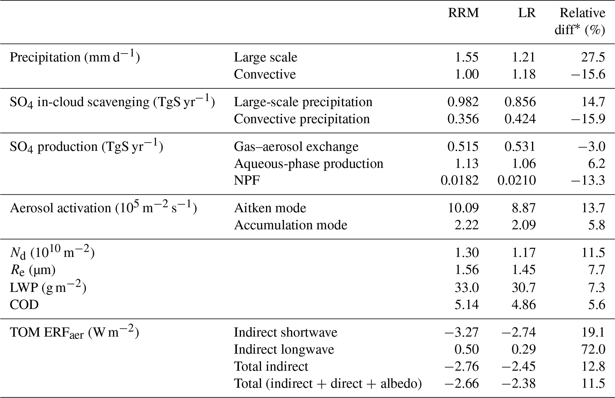
* Relative diff is .
Increasing model horizontal resolution affects the partitioning between large-scale and convective precipitation (Table 2). With more resolved large-scale precipitation and less parameterized deep convective precipitation, in-cloud scavenging of aerosols by large-scale (deep convective) precipitation generally increases (decreases) in the RRM simulation compared to the LR simulation.
RRM enhances the activation of IAPs in large-scale clouds due to the larger temporal variability in the LCLOUD in the RRM simulation compared to the LR simulation (Table 2). Enhanced aerosol activation leads to more cloud droplets. In addition, RRM enhances water vapor condensation, resulting in larger LWP and Re, which leads to larger COD. Since aerosol activation is stronger in the RRM simulation, cloud droplets, LWP, and COD are more sensitive to anthropogenic aerosols. Consequently, the anthropogenic aerosol indirect effect and ERFaer in the RRM are stronger than in the LR simulation (Table 2).
Although the study is limited to comparing the E3SMv1 LR (∼ 100 km) and CONUS RRM (∼ 25 km) simulations, the methodology shown in the study is helpful for future studies to investigate the potential impacts of model resolutions on the simulation results, as RRM is significantly less expensive when computationally compared to the global high-resolution model. Some findings from this study may also apply to E3SM simulations at higher resolutions or even convection-permitting scales, such as the enhancement in natural aerosol emissions due to stronger winds, the partitioning between large-scale and convective precipitation and associated wet scavenging, and improved IAP activation in large-scale clouds. However, we must also emphasize that the aerosol mass budget and ERFaer are sensitive to model configurations and regional characteristics such as aerosol properties, land use and land cover, and climate. Aerosol and clouds in other regions can be very different. Furthermore, some resolution sensitivities may differ as model resolution advances to convection-permitting and subgrid-scale processes become more significant. Moreover, although nudging is applied in the study to minimize the impacts of large-scale circulations on aerosol properties as horizontal resolution changes, differences in meteorology still exist between the RRM and LR simulations (e.g., surface wind speed and precipitation). Therefore, the results above contain the meteorological effect, although the meteorological differences are also caused by the change in horizontal grid spacing.
The E3SMv1 source code is available at https://doi.org/10.11578/E3SM/dc.20180418.36 (E3SM Project, 2018).
We use the Stage IV precipitation data from the MCS–IDC data product, available at https://doi.org/10.25584/1632005 (Li et al., 2020). The LR and RRM simulation results are available at https://doi.org/10.5281/zenodo.7782985 (Li et al., 2023). The level 3 Moderate Resolution Imaging Spectroradiometer (MODIS) gridded (1∘ × 1∘) monthly Dark Target aerosol optical depth (AOD) products used in the Supplement are from https://doi.org/10.5067/MODIS/MOD08_M3.061 (MOD08_M3; Platnick et al., 2015b) and https://doi.org/10.5067/MODIS/MYD08_M3.061 (MYD08_M3; Platnick et al., 2015a). The Aerosol Robotic Network (AERONET) data are available at https://aeronet.gsfc.nasa.gov/new_web/download_all_v3_aod.html (Gupta et al., 2023). The Interagency Monitoring of Protected Visual Environments (IMPROVE) data are available at https://views.cira.colostate.edu/fed/QueryWizard/ (CIRA/CSU, 2023).
The supplement related to this article is available online at: https://doi.org/10.5194/gmd-17-1327-2024-supplement.
KZ and JL designed the study. JL conducted the simulations under the instruction of KZ and with the help of TH, BS, and QY. KZ and SZ determined the nudging strategy, and JL prepared the ERA5 nudging files under the instruction of SZ and KZ. JL performed the analyses, with discussions with KZ, TH, PM, and HH. JL prepared the paper, with contributions from all co-authors.
At least one of the (co-)authors is a member of the editorial board of Geoscientific Model Development. The peer-review process was guided by an independent editor, and the authors also have no other competing interests to declare.
Publisher's note: Copernicus Publications remains neutral with regard to jurisdictional claims made in the text, published maps, institutional affiliations, or any other geographical representation in this paper. While Copernicus Publications makes every effort to include appropriate place names, the final responsibility lies with the authors.
IMPROVE is a collaborative association of state, tribal, and federal agencies and international partners. The U.S. Environmental Protection Agency is the primary funding source, with contracting and research support from the National Park Service. The Air Quality Group at the University of California, Davis, is the central analytical laboratory, with ion analysis provided by Research Triangle Institute and carbon analysis provided by Desert Research Institute. We thank Ilya Slutsker and many other principal investigators or co-principal investigators and their staff for establishing and maintaining the AERONET sites used in the study.
The study has been supported as part of the Enabling Aerosol–cloud interactions at GLobal convection-permitting scalES (EAGLES) project (project no. 74358) sponsored by the United States Department of Energy (DOE), Office of Science, Office of Biological and Environmental Research, Earth System Model Development (ESMD) program area. The Pacific Northwest National Laboratory (PNNL) is operated for the DOE by the Battelle Memorial Institute (under contract no. DE-AC05-76RL01830). The research used high-performance computing resources from the PNNL Research Computing and resources of the National Energy Research Scientific Computing Center (NERSC), a United States Department of Energy, Office of Science User Facility located at Lawrence Berkeley National Laboratory, operated under contract no. DE-AC02-05CH11231, using NERSC awards (grants nos. ALCC-ERCAP0016315, BER-ERCAP0015329, BER-ERCAP0018473, and BER-ERCAP0020990).
This paper was edited by Graham Mann and reviewed by two anonymous referees.
Abdul-Razzak, H. and Ghan, S. J.: A parameterization of aerosol activation: 2. Multiple aerosol types, J. Geophys. Res.-Atmos., 105, 6837–6844, https://doi.org/10.1029/1999JD901161, 2000.
Apte, J. S., Marshall, J. D., Cohen, A. J., and Brauer, M.: Addressing global mortality from ambient PM2.5, Environ. Sci. Technol., 49, 8057–8066, https://doi.org/10.1021/acs.est.5b01236, 2015.
Barth, M., Rasch, P., Kiehl, J., Benkovitz, C., and Schwartz, S.: Sulfur chemistry in the National Center for Atmospheric Research Community Climate Model: Description, evaluation, features, and sensitivity to aqueous chemistry, J. Geophys. Res.-Atmos., 105, 1387–1415, https://doi.org/10.1029/1999JD900773, 2000.
Bogenschutz, P. A., Gettelman, A., Morrison, H., Larson, V. E., Craig, C., and Schanen, D. P.: Higher-order turbulence closure and its impact on climate simulations in the Community Atmosphere Model, J. Climate, 26, 9655-9676, https://doi.org/10.1175/JCLI-D-13-00075.1, 2013.
Burrows, S. M., Easter, R. C., Liu, X., Ma, P.-L., Wang, H., Elliott, S. M., Singh, B., Zhang, K., and Rasch, P. J.: OCEANFILMS (Organic Compounds from Ecosystems to Aerosols: Natural Films and Interfaces via Langmuir Molecular Surfactants) sea spray organic aerosol emissions – implementation in a global climate model and impacts on clouds, Atmos. Chem. Phys., 22, 5223–5251, https://doi.org/10.5194/acp-22-5223-2022, 2022.
Caldwell, P. M., Mametjanov, A., Tang, Q., Van Roekel, L. P., Golaz, J. C., Lin, W., Bader, D. C., Keen, N. D., Feng, Y., and Jacob, R.: The DOE E3SM coupled model version 1: Description and results at high resolution, J. Adv. Model. Earth Sy., 11, 4095–4146, https://doi.org/10.1029/2019MS001870, 2019.
Caldwell, P. M., Terai, C. R., Hillman, B., Keen, N. D., Bogenschutz, P., Lin, W., Beydoun, H., Taylor, M., Bertagna, L., and Bradley, A.: Convection-permitting simulations with the E3SM global atmosphere model, J. Adv. Model. Earth Sy., 13, e2021MS002544, https://doi.org/10.1029/2021MS002544, 2021.
CIRA/CSU: Federal Land Manager Environmental Database, Cooperative Institute for Research in the Atmosphere (CIRA), Colorado State University (CSU) [data set], USA, https://views.cira.colostate.edu/fed/ (last access: 26 May 2022), 2023.
Dennis, J. M., Edwards, J., Evans, K. J., Guba, O., Lauritzen, P. H., Mirin, A. A., St-Cyr, A., Taylor, M. A., and Worley, P. H.: CAM-SE: A scalable spectral element dynamical core for the Community Atmosphere Model, Int. J. High Perform. C., 26, 74–89, https://doi.org/10.1177/1094342011428142, 2012.
Dueben, P. D., Wedi, N., Saarinen, S., and Zeman, C.: Global simulations of the atmosphere at 1.45 km grid-spacing with the Integrated Forecasting System, J. Meteorol. Soc. Jpn. Ser. II, 98, 551–572, https://doi.org/10.2151/jmsj.2020-016, 2020.
E3SM Project, DOE: Energy Exascale Earth System Model v1.0, E3SM Project [code], https://doi.org/10.11578/E3SM/dc.20180418.36, 2018.
Feng, L., Smith, S. J., Braun, C., Crippa, M., Gidden, M. J., Hoesly, R., Klimont, Z., van Marle, M., van den Berg, M., and van der Werf, G. R.: The generation of gridded emissions data for CMIP6, Geosci. Model Dev., 13, 461–482, https://doi.org/10.5194/gmd-13-461-2020, 2020.
Feng, Y., Wang, H., Rasch, P., Zhang, K., Lin, W., Tang, Q., Xie, S., Hamilton, D., Mahowald, N., and Yu, H.: Global dust cycle and direct radiative effect in E3SM version 1: Impact of increasing model resolution, J. Adv. Model. Earth Sy., 14, e2021MS002909, https://doi.org/10.1029/2021MS002909, 2022.
Feng, Z., Song, F., Sakaguchi, K., and Leung, L. R.: Evaluation of Mesoscale Convective Systems in Climate Simulations: Methodological Development and Results from MPAS-CAM over the United States, J. Climate, 34, 2611–2633, https://doi.org/10.1175/JCLI-D-20-0136.1, 2021.
Ghan, S. J.: Technical Note: Estimating aerosol effects on cloud radiative forcing, Atmos. Chem. Phys., 13, 9971–9974, https://doi.org/10.5194/acp-13-9971-2013, 2013.
Golaz, J.-C., Larson, V. E., and Cotton, W. R.: A PDF-based model for boundary layer clouds. Part I: Method and model description, J. Atmos. Sci., 59, 3540–3551, https://doi.org/10.1175/1520-0469(2002)059<3540:APBMFB>2.0.CO;2, 2002.
Golaz, J.-C., Van Roekel, L. P., Zheng, X., Roberts, A. F., Wolfe, J. D., Lin, W., Bradley, A. M., Tang, Q., Maltrud, M. E., and Forsyth, R. M.: The DOE E3SM Model Version 2: overview of the physical model and initial model evaluation, J. Adv. Model. Earth Sy., 14, e2022MS003156, https://doi.org/10.1029/2022MS003156, 2022.
Golaz, J. C., Caldwell, P. M., Van Roekel, L. P., Petersen, M. R., Tang, Q., Wolfe, J. D., Abeshu, G., Anantharaj, V., Asay-Davis, X. S., and Bader, D. C.: The DOE E3SM coupled model version 1: Overview and evaluation at standard resolution, J. Adv. Model. Earth Sy., 11, 2089–2129, https://doi.org/10.1029/2018MS001603, 2019.
Gupta, P., et al.: Aerosol Robotic Network. NASA Goddard Space Flight Center [data set], USA, https://aeronet.gsfc.nasa.gov/ (last access: 26 May 2022), 2023.
Hamilton, D. S., Perron, M. M., Bond, T. C., Bowie, A. R., Buchholz, R. R., Guieu, C., Ito, A., Maenhaut, W., Myriokefalitakis, S., and Olgun, N.: Earth, wind, fire, and pollution: Aerosol nutrient sources and impacts on ocean biogeochemistry, Annu. Rev. Mar. Sci., 14, 303–330, https://doi.org/10.1146/annurev-marine-031921-013612, 2022.
Harris, L. M., Lin, S.-J., and Tu, C.: High-resolution climate simulations using GFDL HiRAM with a stretched global grid, J. Climate, 29, 4293–4314, https://doi.org/10.1175/JCLI-D-15-0389.1, 2016.
Heinzeller, D., Duda, M. G., and Kunstmann, H.: Towards convection-resolving, global atmospheric simulations with the Model for Prediction Across Scales (MPAS) v3.1: an extreme scaling experiment, Geosci. Model Dev., 9, 77–110, https://doi.org/10.5194/gmd-9-77-2016, 2016.
Hersbach, H., Bell, B., Berrisford, P., Hirahara, S., Horányi, A., Muñoz-Sabater, J., Nicolas, J., Peubey, C., Radu, R., and Schepers, D.: The ERA5 global reanalysis, Q. J. Roy. Meteor. Soc., 146, 1999–2049, https://doi.org/10.1002/qj.3803, 2020.
Hoesly, R. M., Smith, S. J., Feng, L., Klimont, Z., Janssens-Maenhout, G., Pitkanen, T., Seibert, J. J., Vu, L., Andres, R. J., Bolt, R. M., Bond, T. C., Dawidowski, L., Kholod, N., Kurokawa, J.-I., Li, M., Liu, L., Lu, Z., Moura, M. C. P., O'Rourke, P. R., and Zhang, Q.: Historical (1750–2014) anthropogenic emissions of reactive gases and aerosols from the Community Emissions Data System (CEDS), Geosci. Model Dev., 11, 369–408, https://doi.org/10.5194/gmd-11-369-2018, 2018.
Hoose, C., Kristjánsson, J. E., Chen, J.-P., and Hazra, A.: A classical-theory-based parameterization of heterogeneous ice nucleation by mineral dust, soot, and biological particles in a global climate model, J. Atmos. Sci., 67, 2483–2503, https://doi.org/10.1175/2010JAS3425.1, 2010.
Hurrell, J. W., Hack, J. J., Shea, D., Caron, J. M., and Rosinski, J.: A new sea surface temperature and sea ice boundary dataset for the Community Atmosphere Model, J. Climate, 21, 5145–5153, https://doi.org/10.1175/2008JCLI2292.1, 2008.
Iacono, M. J., Delamere, J. S., Mlawer, E. J., Shephard, M. W., Clough, S. A., and Collins, W. D.: Radiative forcing by long-lived greenhouse gases: Calculations with the AER radiative transfer models, J. Geophys. Res.-Atmos., 113, D13103, https://doi.org/10.1029/2008JD009944, 2008.
Jickells, T., An, Z., Andersen, K. K., Baker, A., Bergametti, G., Brooks, N., Cao, J., Boyd, P., Duce, R., and Hunter, K.: Global iron connections between desert dust, ocean biogeochemistry, and climate, Science, 308, 67–71, https://doi.org/10.1126/science.1105959, 2005.
Kooperman, G. J., Pritchard, M. S., Ghan, S. J., Wang, M., Somerville, R. C., and Russell, L. M.: Constraining the influence of natural variability to improve estimates of global aerosol indirect effects in a nudged version of the Community Atmosphere Model 5, J. Geophys. Res.-Atmos., 117, D23204, https://doi.org/10.1029/2012JD018588, 2012.
Larson, V. E., Golaz, J.-C., and Cotton, W. R.: Small-scale and mesoscale variability in cloudy boundary layers: Joint probability density functions, J. Atmos. Sci., 59, 3519–3539, https://doi.org/10.1175/1520-0469(2002)059<3519:SSAMVI>2.0.CO;2, 2002.
Li, J., Han, X., Jin, M., Zhang, X., and Wang, S.: Globally analysing spatiotemporal trends of anthropogenic PM2.5 concentration and population's PM2.5 exposure from 1998 to 2016, Environ. Int., 128, 46–62, https://doi.org/10.1016/j.envint.2019.04.026, 2019.
Li, J., Feng, Z., Qian, Y., and Leung, L. R.: MCSs and IDC in the US for 2004–2017, Pacific Northwest National Laboratory DATAHUB [data set], https://doi.org/10.25584/1632005, 2020.
Li, J., Feng, Z., Qian, Y., and Leung, L. R.: A high-resolution unified observational data product of mesoscale convective systems and isolated deep convection in the United States for 2004–2017, Earth Syst. Sci. Data, 13, 827–856, https://doi.org/10.5194/essd-13-827-2021, 2021.
Li, J., Zhang, K., Hassan, T., Zhang, S., Ma, P.-L., Singh, B., Yan, Q., and Huang, H.: Assessing the Sensitivity of Aerosol Mass Budget and Effective Radiative Forcing to Horizontal Grid Spacing in E3SMv1 Using A Regional Refinement Approach – E3SM LR and RRM simulation data, Zenodo [data set], https://doi.org/10.5281/zenodo.7782985, 2023.
Lim, C.-H., Ryu, J., Choi, Y., Jeon, S. W., and Lee, W.-K.: Understanding global PM2.5 concentrations and their drivers in recent decades (1998–2016), Environ. Int., 144, 106011, https://doi.org/10.1016/j.envint.2020.106011, 2020.
Lin, Y. and Mitchell, K. E.: the NCEP stage II/IV hourly precipitation analyses: Development and applications, 19th Conf. Hydrology, American Meteorological Society, San Diego, CA, USA, 2005.
Liu, X., Easter, R. C., Ghan, S. J., Zaveri, R., Rasch, P., Shi, X., Lamarque, J.-F., Gettelman, A., Morrison, H., Vitt, F., Conley, A., Park, S., Neale, R., Hannay, C., Ekman, A. M. L., Hess, P., Mahowald, N., Collins, W., Iacono, M. J., Bretherton, C. S., Flanner, M. G., and Mitchell, D.: Toward a minimal representation of aerosols in climate models: description and evaluation in the Community Atmosphere Model CAM5, Geosci. Model Dev., 5, 709–739, https://doi.org/10.5194/gmd-5-709-2012, 2012.
Liu, X., Ma, P.-L., Wang, H., Tilmes, S., Singh, B., Easter, R. C., Ghan, S. J., and Rasch, P. J.: Description and evaluation of a new four-mode version of the Modal Aerosol Module (MAM4) within version 5.3 of the Community Atmosphere Model, Geosci. Model Dev., 9, 505–522, https://doi.org/10.5194/gmd-9-505-2016, 2016.
Ma, P.-L., Rasch, P. J., Fast, J. D., Easter, R. C., Gustafson Jr., W. I., Liu, X., Ghan, S. J., and Singh, B.: Assessing the CAM5 physics suite in the WRF-Chem model: implementation, resolution sensitivity, and a first evaluation for a regional case study, Geosci. Model Dev., 7, 755–778, https://doi.org/10.5194/gmd-7-755-2014, 2014.
Ma, P. L., Rasch, P. J., Wang, M., Wang, H., Ghan, S. J., Easter, R. C., Gustafson Jr, W. I., Liu, X., Zhang, Y., and Ma, H. Y.: How does increasing horizontal resolution in a global climate model improve the simulation of aerosol-cloud interactions?, Geophys. Res. Lett., 42, 5058–5065, https://doi.org/10.1002/2015GL064183, 2015.
Mahowald, N. M., Scanza, R., Brahney, J., Goodale, C. L., Hess, P. G., Moore, J. K., and Neff, J.: Aerosol deposition impacts on land and ocean carbon cycles, Curr. Clim. Change Rep., 3, 16–31, https://doi.org/10.1007/s40641-017-0056-z, 2017.
Mlawer, E. J., Taubman, S. J., Brown, P. D., Iacono, M. J., and Clough, S. A.: Radiative transfer for inhomogeneous atmospheres: RRTM, a validated correlated-k model for the longwave, J. Geophys. Res.-Atmos., 102, 16663–16682, https://doi.org/10.1029/97JD00237, 1997.
Morrison, H. and Gettelman, A.: A new two-moment bulk stratiform cloud microphysics scheme in the Community Atmosphere Model, version 3 (CAM3). Part I: Description and numerical tests, J. Climate, 21, 3642–3659, https://doi.org/10.1175/2008JCLI2105.1, 2008.
Namikas, S. and Sherman, D. J.: Predicting aeolian sand transport: Revisiting the White model, Earth Surface Processes and Landforms: The J. British Geomorph. Group, 22, 601–604, https://doi.org/10.1002/(SICI)1096-9837(199706)22:6<601::AID-ESP783>3.0.CO;2-5, 1997.
Neale, R. B., Richter, J. H., and Jochum, M.: The impact of convection on ENSO: From a delayed oscillator to a series of events, J. Climate, 21, 5904–5924, https://doi.org/10.1175/2008JCLI2244.1, 2008.
Oleson, K. W., Lawrence, D. M., Bonan, G. B., Drewniak, B., Huang, M., Koven, C. D., Levis, S., Li, F., Riley, W. J., Subin, Z. M., Swenson, S. C., Thornton, P. E., Bozbiyik, A., Fisher, R., Heald, C. L., Kluzek, E., Lamarque, J.-F., Lawrence, P. J., Leung, L. R., Lipscomb, W., Muszala, S., Ricciuto, D. M., Sacks, W., Sun, Y., Tang, J., and Yang, Z.-L.: Technical Description of version 4.5 of the Community Land Model (CLM), National Center for Atmospheric Research, Boulder, Colorado, US, 434, https://doi.org/10.5065/D6RR1W7M, 2013.
Park, S., Bretherton, C. S., and Rasch, P. J.: Integrating cloud processes in the Community Atmosphere Model, version 5, J. Climate, 27, 6821–6856, https://doi.org/10.1175/JCLI-D-14-00087.1, 2014.
Perring, A., Pusede, S., and Cohen, R.: An observational perspective on the atmospheric impacts of alkyl and multifunctional nitrates on ozone and secondary organic aerosol, Chem. Rev., 113, 5848–5870, https://doi.org/10.1021/cr300520x, 2013.
Platnick, S., et al.: MODIS/Aqua Aerosol Cloud Water Vapor Ozone Monthly L3 Global 1Deg CMG. NASA MODIS Adaptive Processing System, Goddard Space Flight Center [data set], USA, https://doi.org/10.5067/MODIS/MYD08_M3.061, 2015a.
Platnick, S., et al.: MODIS/Terra Aerosol Cloud Water Vapor Ozone Monthly L3 Global 1Deg CMG. NASA MODIS Adaptive Processing System, Goddard Space Flight Center [data set], USA, https://doi.org/10.5067/MODIS/MOD08_M3.061, 2015b.
Pusede, S. E., Steiner, A. L., and Cohen, R. C.: Temperature and recent trends in the chemistry of continental surface ozone, Chem. Rev., 115, 3898–3918, https://doi.org/10.1021/cr5006815, 2015.
Qian, Y., Yasunari, T. J., Doherty, S. J., Flanner, M. G., Lau, W. K., Ming, J., Wang, H., Wang, M., Warren, S. G., and Zhang, R.: Light-absorbing particles in snow and ice: Measurement and modeling of climatic and hydrological impact, Adv. Atmos. Sci., 32, 64–91, https://doi.org/10.1007/s00376-014-0010-0, 2015.
Rasch, P., Feichter, J., Law, K., Mahowald, N., Penner, J., Benkovitz, C., Genthon, C., Giannakopoulos, C., Kasibhatla, P., and Koch, D.: A comparison of scavenging and deposition processes in global models: results from the WCRP Cambridge Workshop of 1995, Tellus B, 52, 1025–1056, https://doi.org/10.1034/j.1600-0889.2000.00980.x, 2000.
Rasch, P., Xie, S., Ma, P. L., Lin, W., Wang, H., Tang, Q., Burrows, S., Caldwell, P., Zhang, K., and Easter, R.: An overview of the atmospheric component of the Energy Exascale Earth System Model, J. Adv. Model. Earth Sy., 11, 2377–2411, https://doi.org/10.1029/2019MS001629, 2019.
Ridley, D. A., Heald, C. L., Pierce, J., and Evans, M.: Toward resolution-independent dust emissions in global models: Impacts on the seasonal and spatial distribution of dust, Geophys. Res. Lett., 40, 2873–2877, https://doi.org/10.1002/grl.50409, 2013.
Schwartz, C. S.: Medium-range convection-allowing ensemble forecasts with a variable-resolution global model, Mon. Weather Rev., 147, 2997–3023, https://doi.org/10.1175/MWR-D-18-0452.1, 2019.
Seinfeld, J. H. and Pandis, S. N.: Atmospheric chemistry and physics: from air pollution to climate change, John Wiley & Sons, Inc, Hoboken, New Jersey, ISBN 978-1-118-94740-1, 2016.
Shrivastava, M., Easter, R. C., Liu, X., Zelenyuk, A., Singh, B., Zhang, K., Ma, P. L., Chand, D., Ghan, S., and Jimenez, J. L.: Global transformation and fate of SOA: Implications of low-volatility SOA and gas-phase fragmentation reactions, J. Geophys. Res.-Atmos., 120, 4169–4195, https://doi.org/10.1002/2014JD022563, 2015.
Smith, C. J., Kramer, R. J., Myhre, G., Alterskjær, K., Collins, W., Sima, A., Boucher, O., Dufresne, J.-L., Nabat, P., Michou, M., Yukimoto, S., Cole, J., Paynter, D., Shiogama, H., O'Connor, F. M., Robertson, E., Wiltshire, A., Andrews, T., Hannay, C., Miller, R., Nazarenko, L., Kirkevåg, A., Olivié, D., Fiedler, S., Lewinschal, A., Mackallah, C., Dix, M., Pincus, R., and Forster, P. M.: Effective radiative forcing and adjustments in CMIP6 models, Atmos. Chem. Phys., 20, 9591–9618, https://doi.org/10.5194/acp-20-9591-2020, 2020.
Sun, J., Zhang, K., Wan, H., Ma, P. L., Tang, Q., and Zhang, S.: Impact of nudging strategy on the climate representativeness and hindcast skill of constrained EAMv1 simulations, J. Adv. Model. Earth Sy., 11, 3911–3933, https://doi.org/10.1029/2019MS001831, 2019.
Tang, Q., Klein, S. A., Xie, S., Lin, W., Golaz, J.-C., Roesler, E. L., Taylor, M. A., Rasch, P. J., Bader, D. C., Berg, L. K., Caldwell, P., Giangrande, S. E., Neale, R. B., Qian, Y., Riihimaki, L. D., Zender, C. S., Zhang, Y., and Zheng, X.: Regionally refined test bed in E3SM atmosphere model version 1 (EAMv1) and applications for high-resolution modeling, Geosci. Model Dev., 12, 2679–2706, https://doi.org/10.5194/gmd-12-2679-2019, 2019.
van Marle, M. J. E., Kloster, S., Magi, B. I., Marlon, J. R., Daniau, A.-L., Field, R. D., Arneth, A., Forrest, M., Hantson, S., Kehrwald, N. M., Knorr, W., Lasslop, G., Li, F., Mangeon, S., Yue, C., Kaiser, J. W., and van der Werf, G. R.: Historic global biomass burning emissions for CMIP6 (BB4CMIP) based on merging satellite observations with proxies and fire models (1750–2015), Geosci. Model Dev., 10, 3329–3357, https://doi.org/10.5194/gmd-10-3329-2017, 2017.
Wan, H., Rasch, P. J., Taylor, M. A., and Jablonowski, C.: Short-term time step convergence in a climate model, J. Adv. Model. Earth Syst., 7, 215–225, https://doi.org/10.1002/2014MS000368, 2015.
Wan, H., Zhang, S., Rasch, P. J., Larson, V. E., Zeng, X., and Yan, H.: Quantifying and attributing time step sensitivities in present-day climate simulations conducted with EAMv1, Geosci. Model Dev., 14, 1921–1948, https://doi.org/10.5194/gmd-14-1921-2021, 2021.
Wang, H., Easter, R. C., Rasch, P. J., Wang, M., Liu, X., Ghan, S. J., Qian, Y., Yoon, J.-H., Ma, P.-L., and Vinoj, V.: Sensitivity of remote aerosol distributions to representation of cloud–aerosol interactions in a global climate model, Geosci. Model Dev., 6, 765–782, https://doi.org/10.5194/gmd-6-765-2013, 2013.
Wang, H., Easter, R. C., Zhang, R., Ma, P. L., Singh, B., Zhang, K., Ganguly, D., Rasch, P. J., Burrows, S. M., and Ghan, S. J.: Aerosols in the E3SM Version 1: New developments and their impacts on radiative forcing, J. Adv. Model. Earth Sy., 12, e2019MS001851, https://doi.org/10.1029/2019MS001851, 2020.
Wang, J., Fan, J., Feng, Z., Zhang, K., Roesler, E., Hillman, B., Shpund, J., Lin, W., and Xie, S.: Impact of a new cloud microphysics parameterization on the simulations of mesoscale convective systems in E3SM, J. Adv. Model. Earth Sy., 13, e2021MS002628, https://doi.org/10.1029/2021MS002628, 2021.
Wang, S., Maltrud, M., Elliott, S., Cameron-Smith, P., and Jonko, A.: Influence of dimethyl sulfide on the carbon cycle and biological production, Biogeochemistry, 138, 49–68, https://doi.org/10.1007/s10533-018-0430-5, 2018.
Wang, X., Zhang, R., and Yu, W.: The effects of PM2.5 concentrations and relative humidity on atmospheric visibility in Beijing, J. Geophys. Res.-Atmos., 124, 2235–2259, https://doi.org/10.1029/2018JD029269, 2019.
Wang, Y., Liu, X., Hoose, C., and Wang, B.: Different contact angle distributions for heterogeneous ice nucleation in the Community Atmospheric Model version 5, Atmos. Chem. Phys., 14, 10411–10430, https://doi.org/10.5194/acp-14-10411-2014, 2014.
Xiao, Q., Zheng, Y., Geng, G., Chen, C., Huang, X., Che, H., Zhang, X., He, K., and Zhang, Q.: Separating emission and meteorological contributions to long-term PM2.5 trends over eastern China during 2000–2018, Atmos. Chem. Phys., 21, 9475–9496, https://doi.org/10.5194/acp-21-9475-2021, 2021.
Xie, S., Lin, W., Rasch, P. J., Ma, P. L., Neale, R., Larson, V. E., Qian, Y., Bogenschutz, P. A., Caldwell, P., and Cameron-Smith, P.: Understanding cloud and convective characteristics in version 1 of the E3SM atmosphere model, J. Adv. Model. Earth Sy.s, 10, 2618–2644, https://doi.org/10.1029/2018MS001350, 2018.
Zarzycki, C. M., Levy, M. N., Jablonowski, C., Overfelt, J. R., Taylor, M. A., and Ullrich, P. A.: Aquaplanet experiments using CAM's variable-resolution dynamical core, J. Climate, 27, 5481–5503, https://doi.org/10.1175/JCLI-D-14-00004.1, 2014.
Zender, C. S., Bian, H., and Newman, D.: Mineral Dust Entrainment and Deposition (DEAD) model: Description and 1990s dust climatology, J. Geophys. Res.-Atmos., 108, 4416, https://doi.org/10.1029/2002JD002775, 2003.
Zhang, G. J. and McFarlane, N. A.: Sensitivity of climate simulations to the parameterization of cumulus convection in the Canadian Climate Centre general circulation model, Atmos.-Ocean, 33, 407–446, https://doi.org/10.1080/07055900.1995.9649539, 1995.
Zhang, K., Wan, H., Liu, X., Ghan, S. J., Kooperman, G. J., Ma, P.-L., Rasch, P. J., Neubauer, D., and Lohmann, U.: Technical Note: On the use of nudging for aerosol–climate model intercomparison studies, Atmos. Chem. Phys., 14, 8631–8645, https://doi.org/10.5194/acp-14-8631-2014, 2014.
Zhang, K., Zhang, W., Wan, H., Rasch, P. J., Ghan, S. J., Easter, R. C., Shi, X., Wang, Y., Wang, H., Ma, P.-L., Zhang, S., Sun, J., Burrows, S. M., Shrivastava, M., Singh, B., Qian, Y., Liu, X., Golaz, J.-C., Tang, Q., Zheng, X., Xie, S., Lin, W., Feng, Y., Wang, M., Yoon, J.-H., and Leung, L. R.: Effective radiative forcing of anthropogenic aerosols in E3SM version 1: historical changes, causality, decomposition, and parameterization sensitivities, Atmos. Chem. Phys., 22, 9129–9160, https://doi.org/10.5194/acp-22-9129-2022, 2022a.
Zhang, S., Zhang, K., Wan, H., and Sun, J.: Further improvement and evaluation of nudging in the E3SM Atmosphere Model version 1 (EAMv1): simulations of the mean climate, weather events, and anthropogenic aerosol effects, Geosci. Model Dev., 15, 6787–6816, https://doi.org/10.5194/gmd-15-6787-2022, 2022b.
Zhao, C., Liu, X., Qian, Y., Yoon, J., Hou, Z., Lin, G., McFarlane, S., Wang, H., Yang, B., Ma, P.-L., Yan, H., and Bao, J.: A sensitivity study of radiative fluxes at the top of atmosphere to cloud-microphysics and aerosol parameters in the community atmosphere model CAM5, Atmos. Chem. Phys., 13, 10969–10987, https://doi.org/10.5194/acp-13-10969-2013, 2013.