SERGHEI (SERGHEI-SWE) v1.0: a performance-portable high-performance parallel-computing shallow-water solver for hydrology and environmental hydraulics

The Simulation EnviRonment for Geomorphology, Hydrodynamics, and Ecohydrology in Integrated form (SERGHEI) is a multi-dimensional, multi-domain, and multi-physics model framework for environmental and landscape simulation, designed with an outlook towards Earth system modelling. At the core of SERGHEI's innovation is its performance-portable high-performance parallel-computing (HPC) implementation, built from scratch on the Kokkos portability layer, allowing SERGHEI to be deployed, in a performance-portable fashion, in graphics processing unit (GPU)-based heterogeneous systems. In this work, we explore combinations of MPI and Kokkos using OpenMP and CUDA backends. In this contribution, we introduce the SERGHEI model framework and present with detail its first operational module for solving shallow-water equations (SERGHEI-SWE) and its HPC implementation. This module is designed to be applicable to hydrological and environmental problems including flooding and runoff generation, with an outlook towards Earth system modelling. Its applicability is demonstrated by testing several well-known benchmarks and large-scale problems, for which SERGHEI-SWE achieves excellent results for the different types of shallow-water problems. Finally, SERGHEI-SWE scalability and performance portability is demonstrated and evaluated on several TOP500 HPC systems, with very good scaling in the range of over 20 000 CPUs and up to 256 state-of-the art GPUs.

1 Introduction

The upcoming exascale high-performance parallel-computing (HPC) systems will enable physics-based geoscientific modelling with unprecedented detail (Alexander et al., 2020). Although the need for such HPC systems is traditionally driven by climate, ocean, and atmospheric modelling, hydrological models are progressively becoming as physical, sophisticated, and computationally intensive. Physically based, integrated hydrological models such as Parflow (Kuffour et al., 2020), Amanzi/ATS (Coon et al., 2019), and Hydrogeosphere (Brunner and Simmons, 2012) are becoming more prominent in hydrological research and Earth system modelling (ESM) (Fatichi et al., 2016; Paniconi and Putti, 2015), making HPC more and more relevant for computational hydrology (Clark et al., 2017).

Hydrological models, as with many other HPC applications, are currently facing challenges in exploiting available and future HPC systems. These challenges arise, not only because of the intrinsic complexity of maintaining complex codes over large periods of time, but because HPC and its hardware are undergoing a large paradigm change (Leiserson et al., 2020; Mann, 2020), which is strongly driven by the end of Moore's law (Morales-Hernández et al., 2020). In order to gain higher processing capacity, computers will require heterogeneous and specialised hardware (Leiserson et al., 2020), potentially making high-performing code harder to develop and maintain and demanding that developers adapt and optimise code for an evolving hardware landscape. It has become clear that upcoming exascale systems will have heterogeneous architectures embedded in modular and reconfigurable architectures (Djemame and Carr, 2020; Suarez et al., 2019) that will consist of different types of CPUs and accelerators, possibly from multiple vendors requiring different programming models. This puts pressure on domain scientists to write portable code that performs efficiently on a range of existing and future HPC architectures (Bauer et al., 2021; Lawrence et al., 2018; Schulthess, 2015) and to ensure the sustainability of such code (Gan et al., 2020).

Different strategies are currently being developed to cope with this grand challenge. One strategy is to offload the architecture-dependent parallelisation tasks to the compiler – see, for example, Vanderbauwhede and Takemi (2013); Vanderbauwhede and Davidson (2018); Vanderbauwhede (2021). Another strategy is to use an abstraction layer that provides a unified programming interface to different computational backends – a so-called “performance portability framework” – that allows the same code to be compiled across different HPC architectures. Examples of this strategy include RAJA (Beckingsale et al., 2019) and Kokkos (Edwards et al., 2014; Trott et al., 2021), which are both very similar in their scope and their capability. Both RAJA and Kokkos are C++ libraries that implement a shared-memory programming model to maximise the amount of code that can be compiled across different hardware devices with nearly the same parallel performance. They allow access to several computational backends, in particular multi-graphics processing unit (GPU) and heterogeneous HPC systems.

This paper introduces the Kokkos-based computational (eco)hydrology framework SERGHEI (Simulation EnviRonment for Geomorphology, Hydrodynamics, and Ecohydrology in Integrated form) and its surface hydrology module SERGHEI-SWE. The primary aim of SERGHEI's implementation is scalability and performance portability. In order to achieve this, SERGHEI is written in C++ and based from scratch on the Kokkos abstraction. Kokkos currently supports CUDA, OpenMP, HIP, SYCL, and Pthreads as backends. We chose Kokkos over other alternatives because it is actively engaged in securing the sustainability of its programming model, fostering its partial inclusion into ISO C++ standards (Trott et al., 2021). Indeed, there is an increasing number of applications in multiple domains leveraging on Kokkos – for example, Bertagna et al. (2019); Demeshko et al. (2018); Grete et al. (2021); Halver et al. (2020); Watkins et al. (2020). Thus, among other similar solutions, Kokkos has been identified as advantageous in terms of performance portability and project sustainability, although it is perhaps somewhat more invasive and less clear on the resulting code (Artigues et al., 2019). We present the full implementation of the SERGHEI-SWE module, the shallow-water equations (SWEs) solver for free-surface hydrodynamics at the heart of SERGHEI.

SERGHEI-SWE enables the simulation of surface hydrodynamics of overland flow and streamflow seamlessly and across scales. Historically, hydrological models featuring surface flow have relied on kinematic or zero-inertia (diffusive) approximations due to their apparent simplicity (Caviedes-Voullième et al., 2018; Kollet et al., 2017) and because until the last decade, robust SWE solvers were not available (Caviedes-Voullième et al., 2020a; García-Navarro et al., 2019; Simons et al., 2014; Özgen-Xian et al., 2021). However, the current capabilities of SWE solvers, the increase in computational capabilities, and the need to better exploit parallelism – easier to achieve with explicit solvers than with implicit solvers, as usually required by diffusive equations (Caviedes-Voullième et al., 2018; Fernández-Pato and García-Navarro, 2016) – have been pushing to replace simplified surface flow models (for hydrological purposes) with fully dynamic SWE solvers. There is an increasing number of studies using SWE solvers for rainfall runoff and overland flow simulations from hillslope to catchment scales – for example, Bellos and Tsakiris (2016); Bout and Jetten (2018); Caviedes-Voullième et al. (2012, 2020a); Costabile and Costanzo (2021); Costabile et al. (2021); David and Schmalz (2021); Dullo et al. (2021a, b); Fernández-Pato et al. (2020); García-Alén et al. (2022); Simons et al. (2014); Xia and Liang (2018). This trend contributes to the transition from engineering hydrology towards Earth system science (Sivapalan, 2018), a shift that was motivated by necessity and opportunity, as continental (and larger) ESM will progressively require fully dynamic SWE solvers to cope with increased-resolution digital-terrain models and the dynamics that respond to them, improved spatiotemporal rainfall data and simulations, and increasingly more sophisticated process interactions across scales, from patch to hillslope to catchments (Fan et al., 2019).

Morales-Hernández et al. (2021)Vacondio et al. (2014)Turchetto et al. (2019)Xia et al. (2019)Kobayashi et al. (2015)Carlotto et al. (2021)Shaw et al. (2021)(Bates and Roo, 2000)García-Feal et al. (2018)Caldas Steinstraesser et al. (2021)Kirstetter et al. (2021)Delestre et al. (2017)Wittmann et al. (2017)Moulinec et al. (2011)Berger et al. (2011)Brunner (2021)Simons et al. (2014)Steffen et al. (2020)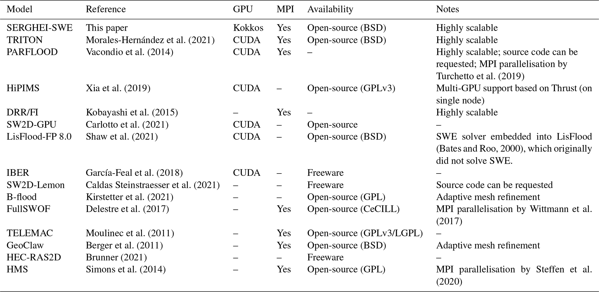

Table 1 Overview of openly available SWE solvers.

SERGHEI-SWE distinguishes itself from other HPC SWE solvers through a number of key novelties. Firstly, SERGHEI-SWE is open sourced under a permissive BSD license. While there are indeed many GPU-enabled SWE codes, many of these are research codes that are not openly available – for example, Aureli et al. (2020); Buttinger-Kreuzhuber et al. (2022); Echeverribar et al. (2020); Hou et al. (2020); Lacasta et al. (2014, 2015); Liang et al. (2016); Vacondio et al. (2017) – or they are commercial codes, such as RiverFlow2D, TUFLOW, HydroAS_2D – see Jodhani et al. (2021) for a recent non-comprehensive review. Open source solvers are a fundamental need for the community, ensuring transparency, reproducibility, and providing a base for model (software) sustainability. We note that open source SWE solvers are becoming increasingly more available – see Table 1. However, only a handful of these freely available models are enabled for GPUs, mostly through CUDA. Fewer of them have multi-GPU capabilities and are capable of fully leveraging HPC hardware. All of these multi-GPU-enabled codes are currently dependent on CUDA and are therefore somewhat limited to Nvidia hardware. This leads into the second and most relevant novelty of SERGHEI-SWE: it is a performance-portable, highly scalable, and GPU-enabled solver. SERGHEI-SWE generalises hardware (CPU, GPU, accelerators) support to a performance-portability concept through Kokkos. This gives SERGHEI-SWE the key advantage of having a single code base for the currently fully operational OpenMP and CUDA backends, as well as HIP, which is currently experimental in SERGHEI but, most importantly, keeps this code base relevant for other backends, such as SYCL. This is particularly important, as the current HPC landscape features not only Nvidia GPUs but also a currently increased adoption of AMD GPUs, with the most recent leading TOP 500 systems – Frontier and LUMI – as well as upcoming systems (e.g. El Capitan) relying on AMD GPUs. In this way, SERGHEI is safely avoiding the vendor lock trap.

SERGHEI-SWE has been developed by harnessing the past 15 years' worth of numerical advances in the solution of SWE, ranging from fundamental numerical formulations (Echeverribar et al., 2019; Morales-Hernández et al., 2020) to HPC GPU implementations (Brodtkorb et al., 2012; Hou et al., 2020; Lacasta et al., 2014, 2015; Liang et al., 2016; Vacondio et al., 2017; Sharif et al., 2020). Most of this work was done in the context of developing solvers for flood modelling, with rather engineering-oriented applications, demanding high quantitative accuracy and predictive capability. Most of the established models in Table 1 were developed within such contexts, although many are currently also adopted for more hydrological applications. Leveraging on this technology, SERGHEI-SWE is designed to cope with the classical shallow-water applications of fluvial and urban flooding, as well as with the emerging rainfall runoff problems in both natural and urban environments (for which coupling to sewer system models is a longer-term objective) and with other flows of broad hydrological and environmental interest that occur on (eco)hydrological timescales, priming it for further uses in ecohydrology and geomorphology. Nevertheless, all shallow-water applications should benefit from the high performance and high scalability of SERGHEI-SWE. With an HPC-ready SWE solver, catchment-scale rainfall runoff applications around the 1 m² resolution are feasible. Similarly, large river and floodplain simulations can be enabled for operational flood forecasting, and flash floods in urban environments can be tackled with extremely high spatial resolution. Moreover, it is noteworthy that SERGHEI-SWE is not confined to HPC environments, and users with workstations can also benefit from improved performance.

1.1 The SERGHEI framework

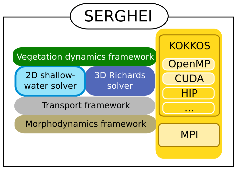
SERGHEI is envisioned as a modular simulation framework around a physically based hydrodynamic core, which allows a variety of water-driven and water-limited processes to be represented in a flexible manner. In this sense, SERGHEI is based on the idea of water fluxes as a connecting thread among various components and processes within the Earth system (Giardino and Houser, 2015). As illustrated by the conceptual framework in Fig. 1, SERGHEI's hydrodynamic core will consist of a mechanistic surface (SERGHEI-SWE, the focus of this paper) and subsurface flow solvers (light and dark blue), around which a generalised transport framework for multi-species transport and reaction will be implemented (grey). The transport framework will further enable the implementation of morphodynamics (gold) and vegetation dynamics (green) models. The transport framework will also include a Lagrangian particle-tracking module (currently also under development). At the time of the writing of this paper, the subsurface flow solver – based on the three-dimensional extension of the Richards solver by Li et al. (2021) – is experimentally operative and is underway to being coupled to the surface flow solver, thus making the hydrodynamic core of SERGHEI applicable to integrated surface–subsurface hydrology. The initial infrastructure for the three other transport-based frameworks is currently under development.

Figure 1 A conceptual framework of SERGHEI.

2 Mathematical and numerical model of SERGHEI-SWE

In this section we provide an overview of the underlying mathematical model and the numerical schemes implemented in SERGHEI-SWE. The implementation is based on well-established numerical schemes, and consequently, we limit this to a minimal presentation.

SERGHEI-SWE is based on the resolution of the two-dimensional (2D) shallow-water equations that can be expressed in a compact differential conservative form as

$$\begin{array}{}\text{(1)}& \left.\begin{array}{r}{\displaystyle \frac{\partial \mathit{U}}{\partial t}}+{\displaystyle \frac{\partial \mathit{F}}{\partial x}}+{\displaystyle \frac{\partial \mathit{G}}{\partial y}}={\mathit{S}}_{\mathrm{r}}+{\mathit{S}}_{\mathrm{b}}+{\mathit{S}}_{\mathrm{f}},\\ {\displaystyle }\mathit{U}=\left[\begin{array}{c}h\\ q_x\\ q_y\end{array}\right]\mathit{F}=\left[\begin{array}{c}{q}_x\\ \frac{q_x^{\mathrm{2}}}{h}+\frac{\mathrm{1}}{\mathrm{2}}g{h}^{\mathrm{2}}\\ \frac{q_x{q}_y}{h}\end{array}\right]\mathit{G}=\left[\begin{array}{c}{q}_y\\ \frac{q_x{q}_y}{h}\\ \frac{q_y^{\mathrm{2}}}{h}+\frac{\mathrm{1}}{\mathrm{2}}g{h}^{\mathrm{2}}\end{array}\right],\\ {\displaystyle }{\mathit{S}}_{\mathrm{r}}=\left[\begin{array}{c}{r}_{\mathrm{o}}-r_{\mathrm{f}}\\ \mathrm{0}\\ \mathrm{0}\end{array}\right]{\mathit{S}}_{\mathrm{b}}=\left[\begin{array}{c}\mathrm{0}\\ -gh\frac{\partial z}{\partial x}\\ -gh\frac{\partial z}{\partial y}\end{array}\right]{\mathit{S}}_{\mathrm{f}}=\left[\begin{array}{c}\mathrm{0}\\ -{\mathit{\sigma }}_x\\ -{\mathit{\sigma }}_y\end{array}\right].\end{array}\right\}\end{array}$$

Here, t [T] is time, x [L] and y [L] are Cartesian coordinates, U is the vector of conserved variables (that is to say the unknowns of the system) containing the water depth, h [L], and the unit discharges in x and y directions, called q_x=hu [L² T⁻¹] and q_y=hv [L² T⁻¹], respectively. F and G are the fluxes of these conserved variables with gravitational acceleration g [L T⁻²]. The mass source terms S_r account for rainfall, r_o [L T⁻¹], and infiltration or exfiltration, r_f [L T⁻¹]. The momentum source terms include gravitational bed slope terms, S_b, expressed according to the gradient of the elevation z [L], and friction terms, S_f, as a function of the friction slope σ. This friction slope is often modelled by means of Gauckler–Manning's equation in terms of Manning's roughness coefficient n [$\mathrm{T}{\mathrm{L}}^{-\mathrm{1}/\mathrm{3}}$] but also frequently with the Chezy and the Darcy–Weisbach formulations (Caviedes-Voullième et al., 2020a). In addition, specialised formulations of the friction slope exist to consider the effect of microtopography and vegetation for small water depths, e.g. variable Manning's coefficients (Jain and Kothyari, 2004; Mügler et al., 2011) or generalised friction laws (Özgen et al., 2015b). A recent systematic comparison and in-depth discussion of several friction models with a focus on rainfall runoff simulations is given in Crompton et al. (2020). Implementing additional friction models is of course possible – and relevant, especially to address the multiscale nature of runoff in catchments – but not essential to the points in this paper. The observant reader will note that in Eq. (1), viscous and turbulent fluxes have been neglected. The focus here is on applications (rainfall runoff, dam breaks) where the influence of these can be safely neglected. Turbulent viscosity may become significant for ecohydraulic simulations of river flow, and turbulent fluxes of course play an important role in mixing in transport simulations. We will address these issues in future implementations of the transport solvers in SERGHEI.

SERGHEI-SWE uses a first-order accurate upwind finite-volume scheme with a forward Euler time integration to solve the system of Eq. (1) on uniform Cartesian grids with grid spacing Δx [L]. The numerical scheme, presented in detail in Morales-Hernández et al. (2021), harnesses many solutions that have been reported in the literature in the past decade, ensuring that all desirable properties of the scheme (well-balancing, depth positivity, stability, robustness) are preserved under the complex conditions of realistic environmental problems. In particular, we require the numerical scheme to stay robust and accurate in the presence of arbitrary rough topography and shallow-water depths with wetting and drying.

Well-balancing and water depth positivity are ensured by solving numerical fluxes at each cell edge k with augmented Riemann solvers (Murillo and García-Navarro, 2010, 2012) based on the Roe linearisation (Roe, 1981). In fluctuation form, the rule for updating the conserved variables in cell i from time step n to time step n+1 reads as follows:

$$\begin{array}{}\text{(2)}& {\mathit{U}}_i^{\ast }={\mathit{U}}_i^n-{\displaystyle \frac{\mathrm{\Delta }t}{\mathrm{\Delta }x}}\sum _{k=\mathrm{1}}^{\mathrm{4}}\sum _{m=\mathrm{1}}^{\mathrm{3}}{\displaystyle \frac{{\stackrel{\mathrm{̃}}{\mathit{\lambda }}}^{-}}{\stackrel{\mathrm{̃}}{\mathit{\lambda }}}}{\left[(\stackrel{\mathrm{̃}}{\mathit{\lambda }}\stackrel{\mathrm{̃}}{\mathit{\alpha }}-\stackrel{\mathrm{̃}}{\mathit{\beta }})\stackrel{\mathrm{̃}}{\mathit{e}}\right]}_{m,k}^n,\end{array}$$

followed by

$$\begin{array}{}\text{(3)}& {\mathit{U}}_i^{n+\mathrm{1}}={\mathit{U}}_i^{\ast }+(r_{\mathrm{o}}-r_{\mathrm{f}}{)}_i^n\mathrm{\Delta }t,\end{array}$$

where $\stackrel{\mathrm{̃}}{\mathit{\lambda }}$ and $\stackrel{\mathrm{̃}}{\mathit{e}}$ are the eigenvalues and eigenvectors of the linearised system of equations, $\stackrel{\mathrm{̃}}{\mathit{\alpha }}$ and $\stackrel{\mathrm{̃}}{\mathit{\beta }}$ are the fluxes and bed slope and friction source term linearisations, respectively, and the minus sign accounts for the upwind discretisation. Note that all the tilde variables are defined at each computational edge. The time step Δt is restricted to ensure stability, following the Courant–Friedrichs–Lewy (CFL) condition:

$$\begin{array}{}\text{(4)}& \begin{array}{rl}\mathrm{\Delta }t=& \text{CFL}\underset{i}{min}\left\{{\displaystyle \frac{\mathrm{\Delta }x}{{\left|{\displaystyle \frac{q_x}{h}}\right|}_i+{\sqrt{gh}}_i,{\left|{\displaystyle \frac{q_y}{h}}\right|}_i+\sqrt{g{h}_i}}}\right\}\\ & \mathrm{\text{ CFL}}\le \mathrm{0.5}.\end{array}\end{array}$$

Although the wave speed values are formally defined at the interfaces, the corresponding cell values are used instead for the CFL condition. As pointed in Morales-Hernández et al. (2021), this approach does not compromise the stability of the system but accelerates the computations and simplifies the implementation.

It is relevant to acknowledge that second (and higher)-order schemes for SWE are available (e.g. Buttinger-Kreuzhuber et al., 2019; Caviedes-Voullième et al., 2020b; Hou et al., 2015; Navas-Montilla and Murillo, 2018). However, first-order schemes are still a pragmatic choice (Ayog et al., 2021), especially when dealing with very high resolutions (as targeted with SERGHEI), which offsets their higher discretisation error and numerical diffusivity in comparison to higher-order schemes. Similarly, robust schemes for unstructured triangular meshes are well established together with their well-known advantages in reducing cell counts and numerical diffusion (Bomers et al., 2019; Caviedes-Voullième et al., 2012, 2020a). As these advantages are less relevant at very high resolutions, we opt for Cartesian grids to avoid issues with memory mapping, coalescence and cache misses in GPUs (Lacasta et al., 2014), and additional memory footprints while also making domain decomposition simpler. Both higher-order schemes and unstructured (and adaptive) meshes may also be implemented within SERGHEI.

3 HPC implementation of the SERGHEI framework

In this section we describe the key ingredients of the HPC implementation of SERGHEI. Conceptually, this requires, firstly, handling parallelism inside a computational device (multicore CPU or GPU) with shared memory and the related portability and corresponding backends (i.e. OpenMP, CUDA, HIP, etc.). On a higher level of parallelism, distributing computations across many devices requires domain decomposition and a distributed memory problem, implemented via MPI. The complete implementation of SERGHEI encompasses both, distributing parallel computations into many subdomains, each of which is mapped onto a computational device. Here we start the discussion from the higher level of domain decomposition and highlight that the novelty of SERGHEI lies with the multiple levels of parallelism together with the performance-portable shared-memory approach via Kokkos.

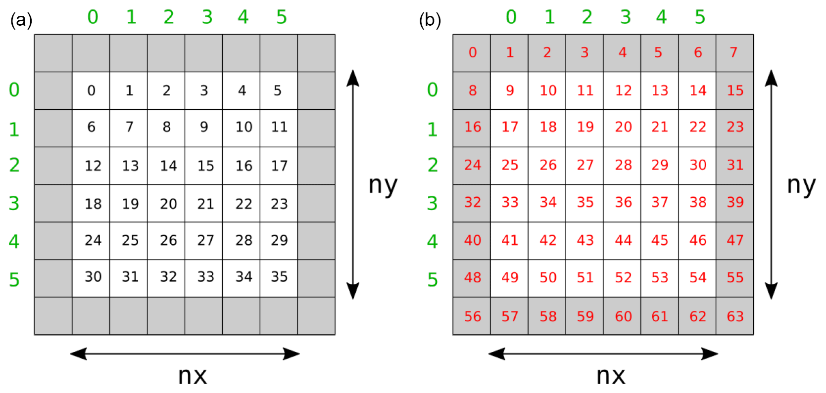
Figure 2 Domain decomposition and indexing in SERGHEI: a subdomain consists of physical cells (white) and halo cells (grey). SERGHEI uses two sets of indices: an index for physical cells (a) and an index for all cells including the halo cells (b).

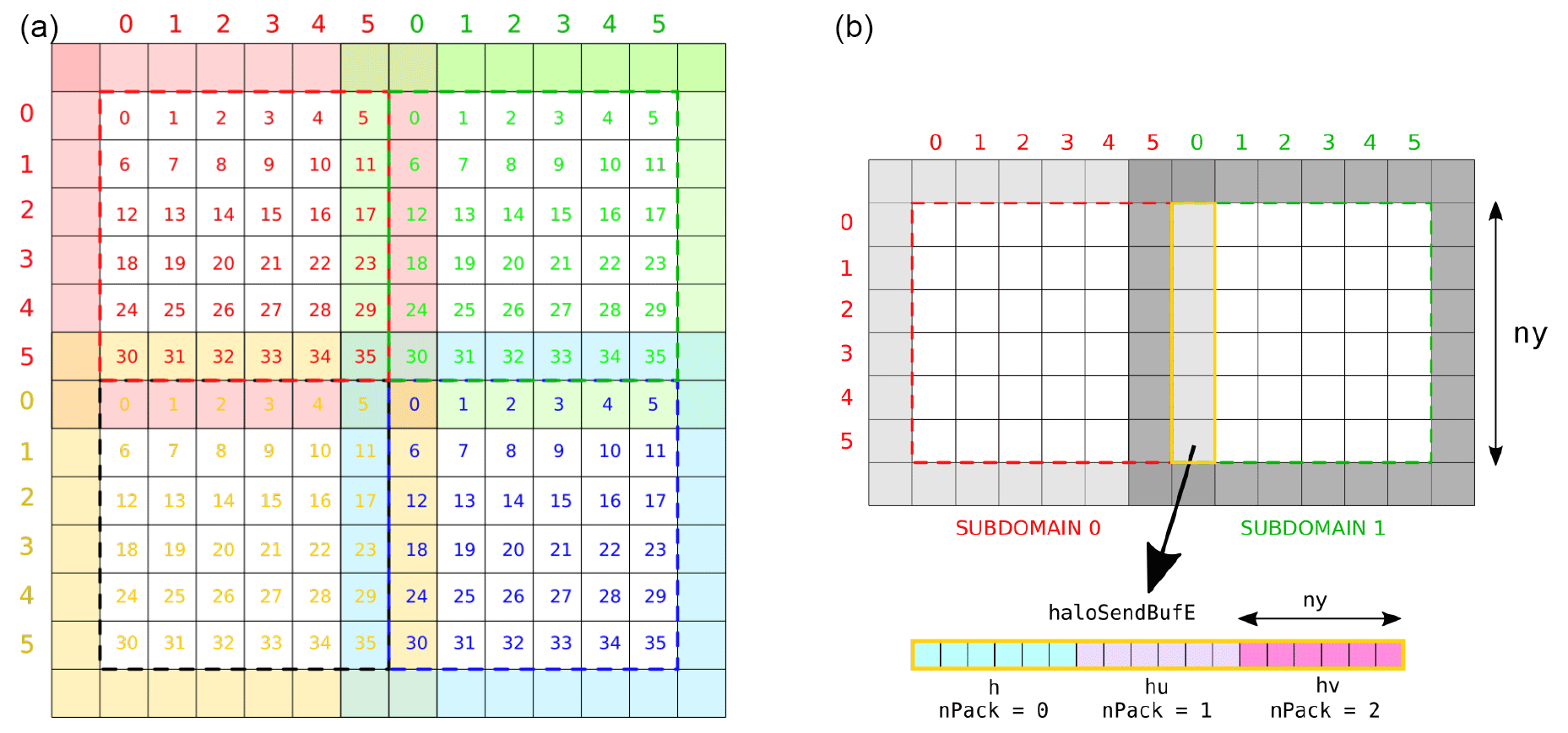
Figure 3 Data exchange between subdomains in SERGHEI: in the global surface domain, subdomains overlap with each other through their halo cells (a). These halo cells are used to exchange data between the subdomains (b).

3.1 Domain decomposition

The surface domain is a two-dimensional plane, discretised by a Cartesian grid with a total cell number of N_t=N_xN_y, where N_x and N_y are the number of cells in x and y directions, respectively. Operations are usually performed per subdomain, each one associated with an MPI rank. During initialisation, each MPI process constructs a local subdomain with n_x cells in x direction and n_y cells in y direction. The user specifies the number of subdomains in each Cartesian direction at runtime, and SERGHEI determines the subdomain size from this information. Subdomains are the same size, except for correction due to non-integer-divisible decompositions. In order to communicate information across subdomains, SERGHEI uses so-called “halo cells”, non-physical cells on the boundaries of the subdomain that overlap with physical cells from neighbouring subdomains. The halo cells augment the number of cells in x and y direction by 1 at each boundary. Thus, the subdomain size is $n_t=(n_x+\mathrm{2})(n_y+\mathrm{2})$. The definitions are sketched – without loss of generality – for a square-shaped subdomain in Fig. 2, and the way these subdomains overlap in the global domain is sketched in Fig. 3 (left). Halo cells are not updated as part of the time stepping. Instead, they are updated by receiving data from the neighbouring subdomain, a process which naturally requires MPI communications.

Besides the global cell index that ranges from 0 to N_t, each subdomain uses two sets of local indices to access data stored in its cells. The first set spans over all physical cells inside the subdomain, and the second index spans over both halo cells and physical cells – see Fig. 2. The second set maps into memory position. For example, in order to access the physical cell 14 in Fig. 2, one has to access memory position 27.

3.2 Data exchange between subdomains

The underlying methods for data exchange between subdomains are centred on the subdomains rather than on the interfaces. Data are exchanged through MPI-based send-and-receive calls (non-blocking) that aggregate data in the halo cells across the subdomains. Note that, by default, Kokkos implicitly assumes that the MPI library is GPU aware, allowing GPU-to-GPU communication provided that the MPI libraries support this feature. Figure 3 (right) illustrates the concept of sending a halo buffer containing state variables from subdomain 1 to update halo cells of subdomain 0. The halo buffer contains state variables for n_y cells, grouped as water depth (h), unit discharge in x direction (hu), and unit discharge in y direction (hv).

3.3 Performance-portable implementation

Intra-device parallelism is achieved per subdomain through the Kokkos framework, which allows the user to choose between shared-memory parallelism and GPU backends for further acceleration. SERGHEI's implementation makes use of the Kokkos concept of Views, which are memory-space-aware abstractions. For example, for arrays of real numbers, SERGHEI defines a type realArr, based on View. This takes the form of Listing 1 for the shared (host) memory space and Listing 2 for the unified virtual memory (UVM) GPU device CUDA memory space. The UVM significantly facilitates development while avoiding writing explicit host-to-device (and vice versa) memory movements.

Listing 1 realArr definition based on View for CPU.

For a CUDA backend, the use of unified memory (CudaUVMSpace) is shown in Listing 2.

Listing 2 realArr definition based on View for GPU.

Similar definitions can be constructed for integer arrays. These arrays describe spatially distributed fields, such as conserved variables, model parameters, and forcing data. Deriving these arrays from View allows us to operate on them via Kokkos to achieve performance portability.

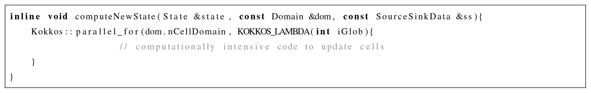
Conceptually, the SERGHEI-SWE solver consists of two computationally intensive kernels: (i) cell-spanning and (ii) edge-spanning kernels. The update of the conserved variables following Eq. (2) results in a kernel around a cell-spanning loop. These cell-spanning loops are the most frequent ones in SERGHEI-SWE and are used for many processes of different computational demand. The standard C++ implementation of such a kernel is illustrated in Listing 3, which spans indices i and j of a 2D Cartesian grid. Here, the loops may be parallelised using, for example, OpenMP or CUDA. However, such a direct implementation of, for example, an OpenMP parallelisation would not automatically allow leveraging GPUs. That is to say, such an implementation is not portable.

Listing 3 Conserved variable update in standard C++.

In order to achieve the desired portability, we replace the standard for by a Kokkos::parallel_for, which enables a lambda function, is minimally intrusive, and reformulates this kernel to the code shown in Listing 4. As a result, this implementation can be compiled for both OpenMP applications and GPUs with Kokkos handling the low-level parallelism on different backends.

Listing 4 Conserved variable update using Kokkos.

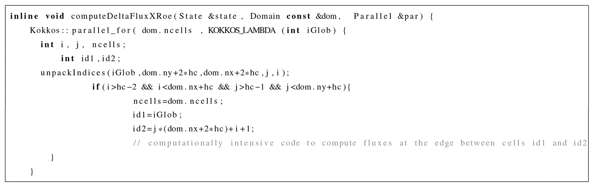
Edge-spanning loops are conceptually necessary to compute numerical fluxes (Eq. 2). Although numerical fluxes can be computed in a cell-centred fashion, this would lead to inefficiencies due to duplicated computations. In Listing 5 we illustrate the edge-spanning kernel solving the numerical fluxes in SERGHEI-SWE. Notably, Listing 5 is indexed by cells, and the construction of edge-wise tuples occurs inside of the kernel. This bypasses the need for additional memory structures to hold edge-based information, but only for Cartesian meshes. Generalisation to adaptive or unstructured meshes would require explicitly an edge-based loop with an additional View of size equal to the number of edges.

Listing 5 Flux computations.

Figure 4 Lake at rest solution for emerged bump. SERGHEI-SWE satisfies the C property.

4 Verification and validation

In this section we report evidence supporting the claim that SERGHEI-SWE is an accurate, robust and efficient shallow-water solver. The formal accuracy testing strategy is based on several well-known benchmark cases with well-defined reference solutions. Herein, for brevity, we focus only on the results of these tests, while providing a minimal presentation of the set-ups. We refer the interested reader to the original publications (and to the many instances in which these tests have been used) for further details on the geometries, parametrisations and forcing.

We purposely report an extensive testing exercise to show the wide applicability of SERGHEI across hydraulic and hydrological problems, with a wide range of the available benchmark tests. Analytical, experimental and field-scale tests are included. The first are aimed at showing formal convergence and accuracy. The experimental cases are meant as validation of the capabilities of the model to reach physically meaningful solutions under a variety of conditions. The field-scale tests showcase the applicability of the solver for real problems, and allow for strenuous computational tasks to show performance, efficiency, and parallel scaling. All solutions reported here were computed using double precision arithmetic.

4.1 Analytical steady flows

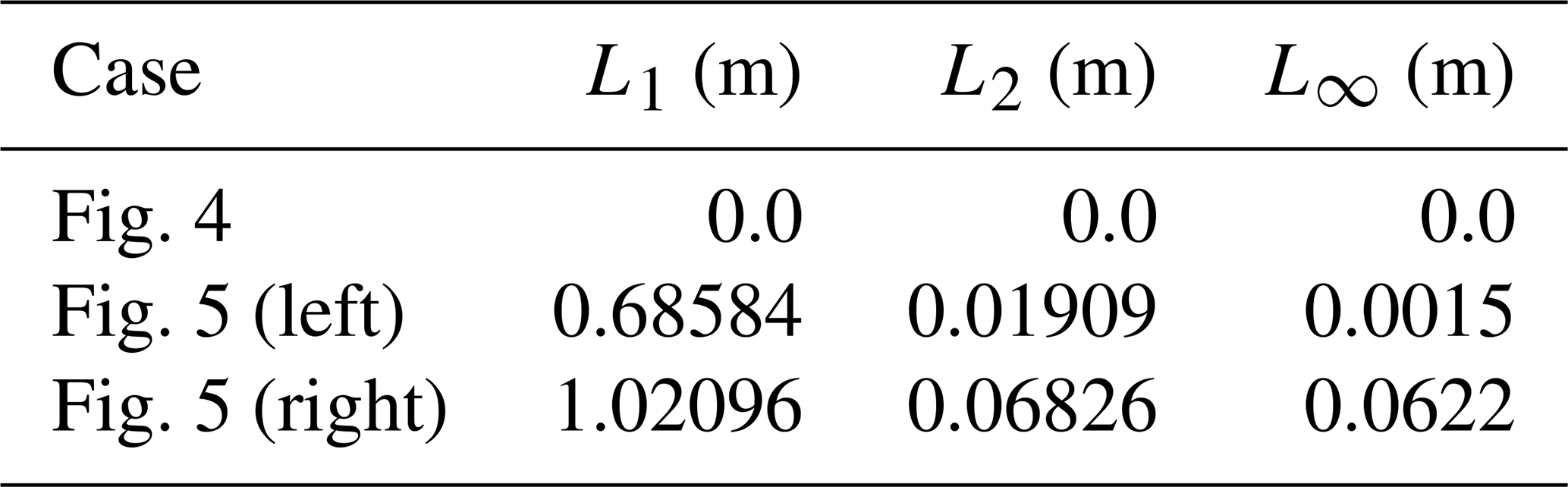
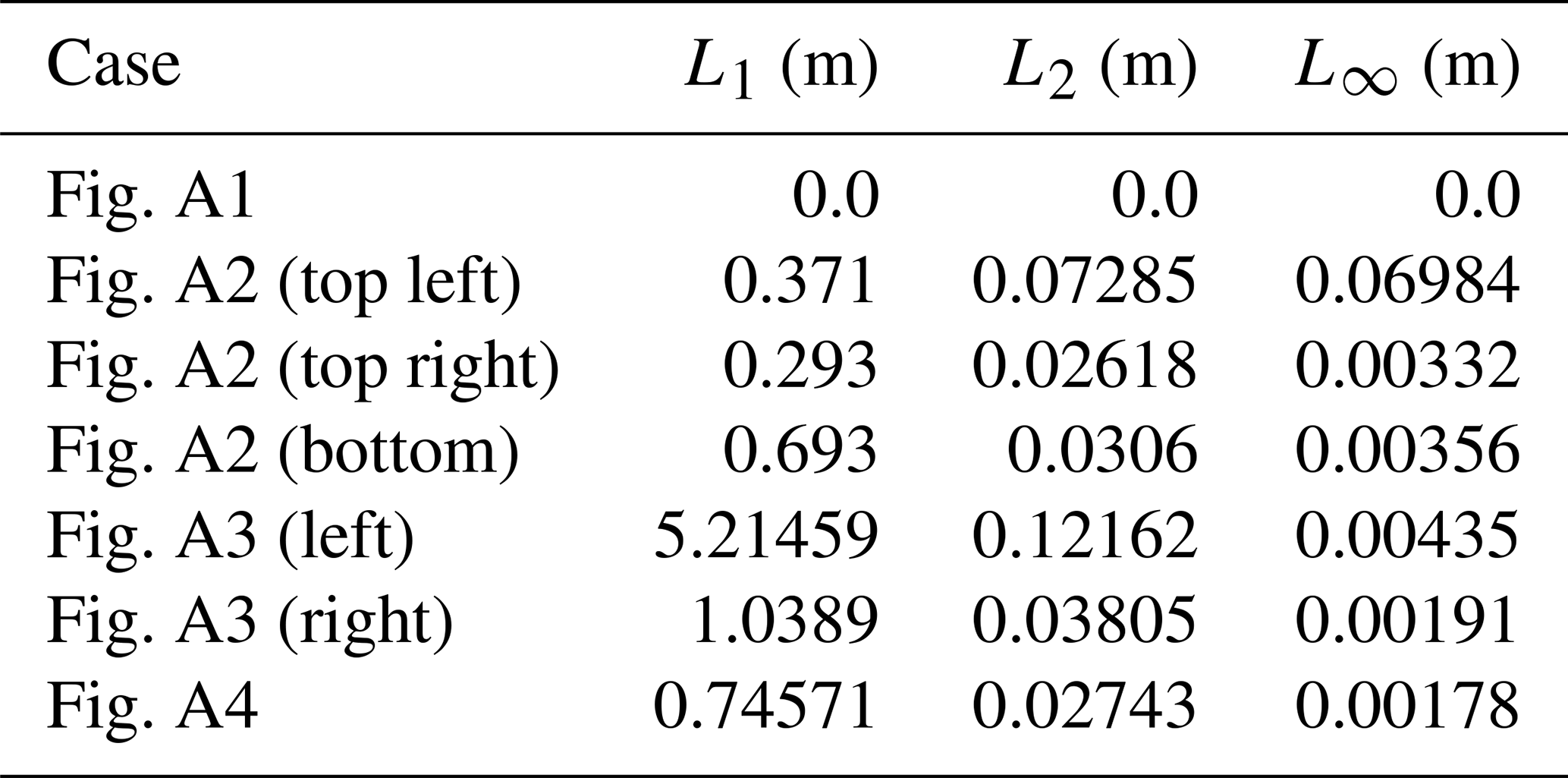
We test SERGHEI's capability to capture moving equilibria in a number of steady-flow test cases compiled in Delestre et al. (2013). Details of the test cases for reproduction purposes can be retrieved from Delestre et al. (2013) and the accompanying software, SWASHES – in this work, we use SWASHES version 1.03. In the following test cases, the domain is always discretised using 1000 computational cells. A summary of L norms for all test cases is given in Table 2. The definition of the L norms is given in Appendix A.

Table 2 Analytical steady flows: summary of L norms for errors in water depth; L norms for errors in unit discharge are in the range of machine accuracy and omitted here.

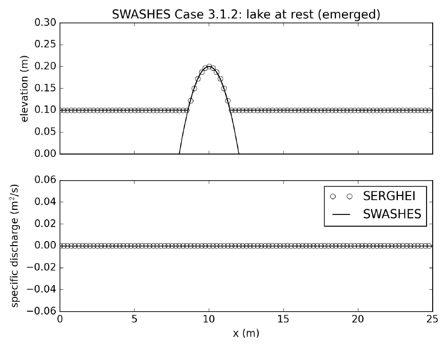
4.1.1 C property

These tests feature a smooth bump in a one-dimensional, frictionless domain which can be used to validate the C property, well-balancing, and the shock-capturing ability of the numerical solver (Morales-Hernández et al., 2012; Murillo and García-Navarro, 2012). Figure 4 shows that SERGHEI-SWE satisfies the C property by preserving a lake at rest in the presence of an emerged bump (an immersed bump test is shown in Sect. A1) and matches the analytical solution provided by SWASHES.

4.1.2 Well-balancing

To show well-balancing under steady flow, we computed two transcritical flows based on the analytical benchmark of a one-dimensional flume with varying geometry proposed by MacDonald et al. (1995). These tests are well known and widely used as benchmark solutions (e.g. Caviedes-Voullième and Kesserwani, 2015; Delestre et al., 2013; Kesserwani et al., 2019; Morales-Hernández et al., 2012; Murillo and García-Navarro, 2012). Additional well-balancing tests can be found in Sect. A2. At steady state, local acceleration terms and source terms balance each other out such that the free surface water elevation becomes a function of bed slope and friction source terms. Thus, these test cases can be used to validate the implementation of these source terms and the well-balanced nature of the complete numerical scheme. This is particularly important to subcritical fluvial flows and rainfall runoff problems, since both are usually dominated by these two terms.

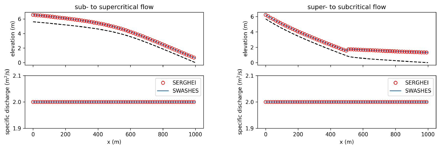
Figure 5 Analytical steady flows: flumes. SERGHEI-SWE captures moving equilibria solutions for two transcritical steady flows. Note that the solution is stable (no oscillations) and well-balanced (discharge remains constant along the flume).

Table 3 Analytical dam break: L norms and empirical convergence rates (R) for water depth (h) and velocity (u).

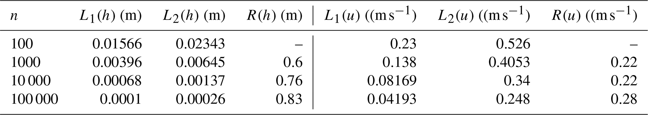
Figure 5 shows comparisons between SERGHEI-SWE and analytical solutions (obtained through SWASHES) for two transcritical steady flows. Very good agreement is obtained. Note that the unit discharge is captured with machine accuracy in the presence of friction and bottom changes, which is mainly due to the upwind friction discretisation used in the SERGHEI-SWE solver. As reported by Burguete et al. (2008) and Murillo et al. (2009), a centred friction discretisation does not ensure a perfect balance between fluxes and source terms for steady states even if using the improved discretisation by Xia et al. (2017).

4.2 Analytical dam break

We verify SERGHEI-SWE's capability to capture transient flow based on analytical dam breaks (Delestre et al., 2013). Dam break problems are defined by an initial discontinuity in the water depth in the domain h(x), such that

$$\begin{array}{}\text{(5)}& h\left(x\right)=\left\{\begin{array}{ll}{h}_{\mathrm{L}}& \text{if }x\le x_{\mathrm{0}},\\ h_{\mathrm{R}}& \text{otherwise},\end{array}\right.\end{array}$$

where h_L denotes a specified water depth on the left-hand side of the location of the discontinuity x₀, and h_R denotes the specified water depth on the right-hand side of x₀. The domain is 10 m long, the discontinuity is located at x₀ = 5 m, and the total run time is 6 s. Initial velocities are nil in the entire domain. In the following, we report empirical evidence of the numerical-schemes mesh convergence property by comparing model predictions for test cases with 100, 1000, 10 000, and 100 000 elements, respectively.

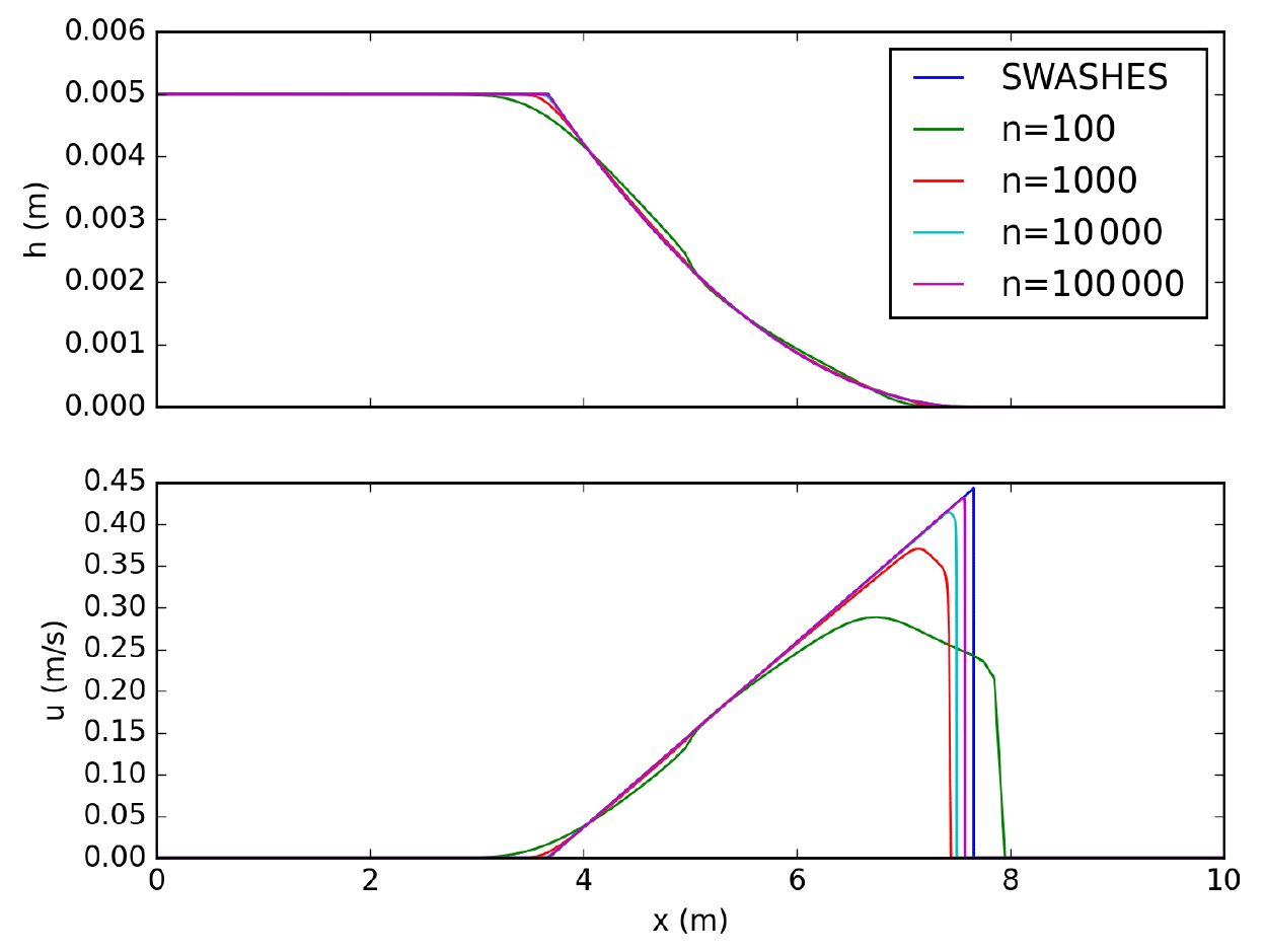
Figure 6 Dam break on dry bed without friction: model predictions for different number of grid cells. SERGHEI-SWE converges to the analytical solution (Ritter's solution) as the grid is refined.

A classical frictionless dam break over a wet bed is reported in Sect. A3. Here we focus on a frictionless dam break over a dry bed. Flow featuring depth close to dry bed is a special case for the numerical solver because regular wave speed estimations become invalid Toro (2001). Initial conditions are set as h_L = 0.005 m and h_R = 0 m. Model results are plotted against the analytical solution by Ritter for different grid resolutions in Fig. 6. The model results converge to the analytical solution as the grid is refined. This is also seen in Table 3, where errors and convergence rates for this test case are summarised. Note that the norms definition can be found in Sect. A2. The observed convergence rate is below the theoretical convergence rate of R=1 because of the increased complexity introduced by the discontinuity in the solution and the presence of dry bed.

4.3 Analytical oscillation: parabolic bowl

We present transient two-dimensional test cases with moving wet–dry fronts that consider the periodical movement of water in a parabolic bowl, so-called “oscillations” that have been studied by Thacker (1981). We replicate two cases from the SWASHES compilation (Delestre et al., 2013), using a mesh spacing of Δx = 0.01 m, one reported here and the other in Sect. A4.

The well-established test case by Thacker (1981) for a periodic oscillation of a planar surface in a frictionless paraboloid has been extensively used for validation of shallow-water solvers (e.g. Aureli et al., 2008; Dazzi et al., 2018; Liang et al., 2015; Murillo and García-Navarro, 2010; Vacondio et al., 2014; Zhao et al., 2019) because of its rather complex 2D nature and the presence of moving wet–dry fronts. The topography is defined as

$$\begin{array}{}\text{(6)}& \begin{array}{rl}& z\left(r\right)=-h_{\mathrm{0}}\left(\mathrm{1}-{\displaystyle \frac{r^{\mathrm{2}}}{a^{\mathrm{2}}}}\right),\\ & r=\sqrt{(x-L/\mathrm{2}{)}^{\mathrm{2}}+(y-L/\mathrm{2}{)}^{\mathrm{2}}},\end{array}\end{array}$$

where r is the radius, h₀ is the water depth at the centre of the paraboloid, a is the distance from the centre to the zero-elevation shoreline, L is the length of the square-shaped domain, and x and y denote coordinates inside the domain. The analytical solution is derived in Thacker (1981). We use the same values as Delestre et al. (2013), that is h₀ = 0.1 m, a = 1 m, and L = 4 m. The simulation is run for three periods (T = 2.242851 s), with a spatial resolution of δx = 0.01 m. The analytical solution can be found in Thacker (1981); Delestre et al. (2013).

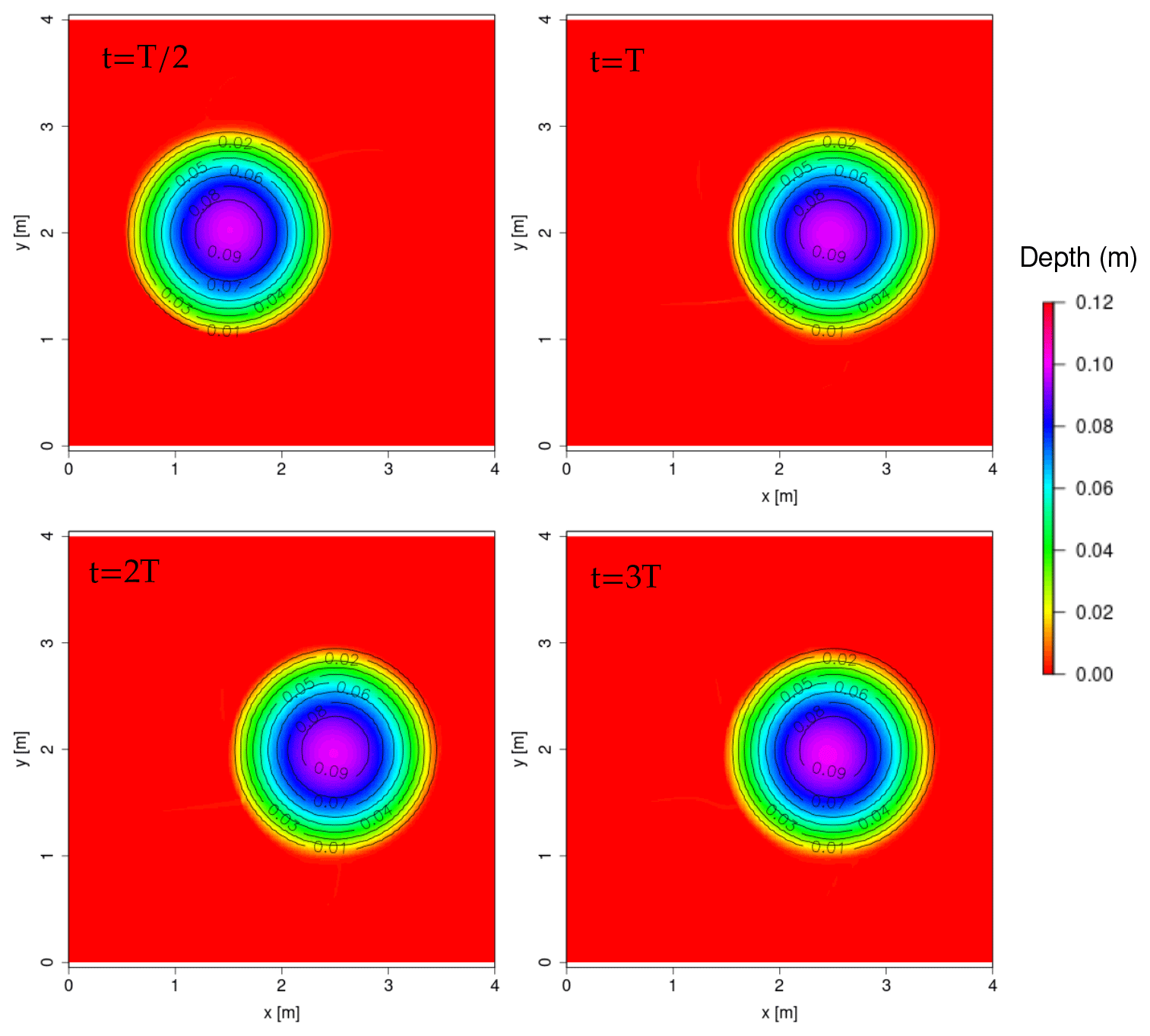
Figure 7 Planar surface in a paraboloid: snapshots of water depth by the model compared to the analytical solution (contour lines). Period T = 2.242851 s.

Snapshots of the simulation are plotted in Fig. 7 and compared to the analytical solution. The model results agree well with the analytical solution after three periods, with slight growing-phase error, as is commonly observed on this test case.

4.4 Variable rainfall over a sloping plane

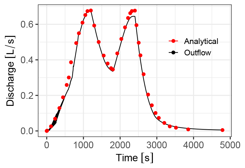
Govindaraju et al. (1990) presented an analytical solution to a time-dependent rainfall over a sloping plane, which is commonly used (Caviedes-Voullième et al., 2020a; Gottardi and Venutelli, 2008; Singh et al., 2015). The plane is 21.945 m long, with a slope of 0.04. We select rainfall B from Govindaraju et al. (1990), a piecewise constant rainfall with two periods of alternating low and high intensities (50.8 and 101.6 mm h⁻¹) up until 2400 s. Friction is modelled with Chezy's equation, with a roughness coefficient of 1.767 ${\mathrm{m}}^{\mathrm{1}/\mathrm{2}}{\mathrm{s}}^{-\mathrm{1}}$. The computational domain was defined by a 200 × 10 grid, with δx = 0.109725 m.

The simulated discharge hydrograph at the outlet is compared against the analytical solution in Fig. 8. The numerical solutions matches the analytical one very well. The only relevant difference occurs in the magnitude of the second discharge peak, which is slightly underestimated in the simulation.

Figure 8 Simulated and analytical discharge for the analytical case of rainfall in a flume.

5 Laboratory-scale experiments

5.1 Experimental steady and dam break flows over complex geometry

Martínez-Aranda et al. (2018) presented experimental results of steady and transient flows over several obstacles while recording transient 3D water surface elevation in the region of interest. We selected the so-called G3 case and simulated both a dam break and steady flow. The experiment took place in a double-sloped plexiglass flume, 6 m long and 24 cm wide. The obstacles in this case are a symmetric contraction and a rectangular obstacle on the centreline, downstream of the contraction.

For both cases the flume (including the upstream wider reservoir) was discretised at a 5 mm resolution, resulting in a computational domain with 106 887 cells. Manning's roughness was set to 0.01 $\mathrm{s}{\mathrm{m}}^{-\mathrm{1}/\mathrm{3}}$. The steady simulation was run from an initial state with uniform depth h = 5 cm up to t = 300 s. The dam break simulation duration was 40 s.

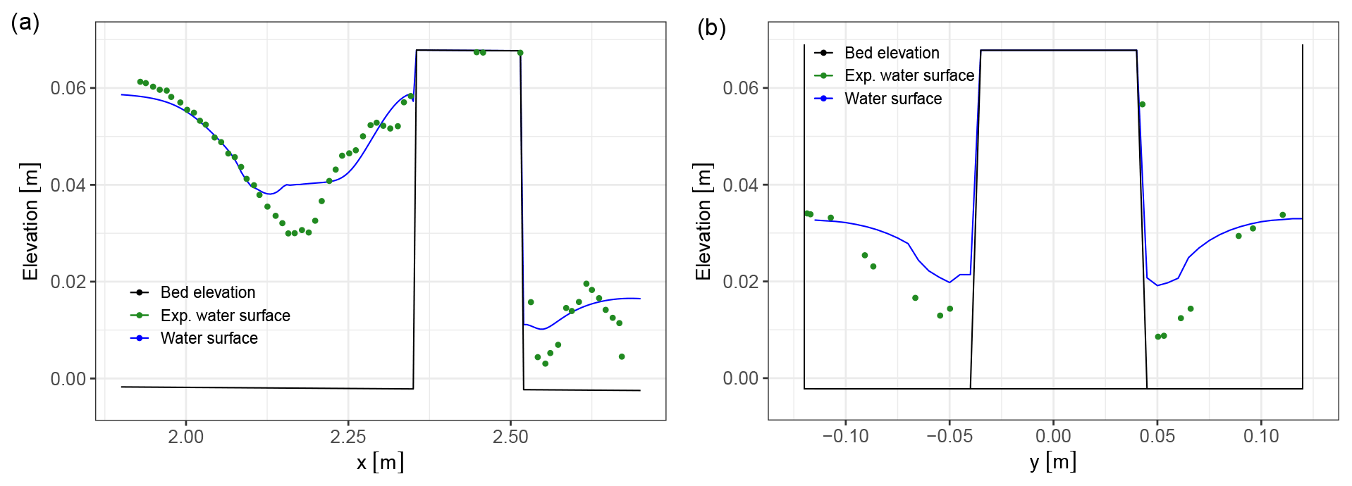
Figure 9 Simulated and experimental steady water surface in the obstacle region of the G3 flume for the centreline profile y = 0 m (a) and a cross-section x = 2.40 m (b).

The steady-flow case had a discharge of 2.5 L s⁻¹. Steady water surface results in the obstacle region are shown in Fig. 9 for a centreline profile (y=0) and a cross-section at the rectangular obstacle, specifically at x = 2.40 m (the coordinate system is set at the centre of the flume inlet gate). The simulation results approximate experimental results well. The mismatches are similar to those analysed by Martínez-Aranda et al. (2018) and can be attributed to turbulent and 3D phenomena near the obstacles.

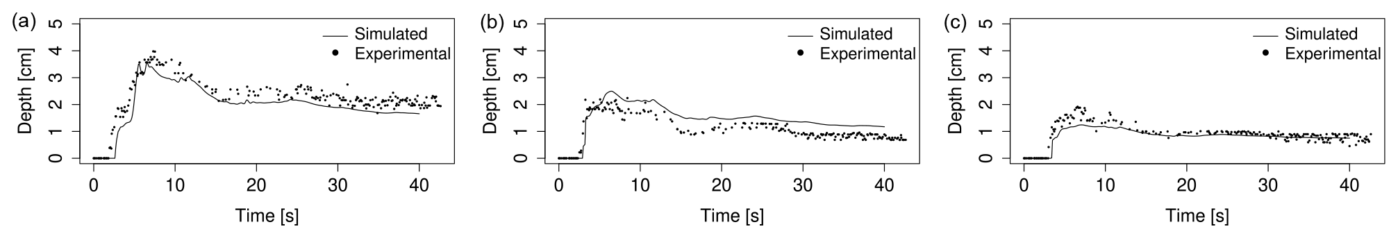
Figure 10 Simulated and experimental transient water depths at three gauge points (a x = 2.25 m, y = 0 m; b x = 2.40 m, y = 0.08 m; c x = 2.60 m, y = 0 m) for the G3 flume dam break over several obstacles.

The dam break case is triggered by a sudden opening of the gate followed by a wave advancing along the dry flume. Results for this case at three gauge points are shown in Fig. 10. Again, the simulations approximate experiments well, capturing both the overall behaviour of the water depths and the arrival of the dam break wave, with local errors attributable to the violent dynamics (Martínez-Aranda et al., 2018).

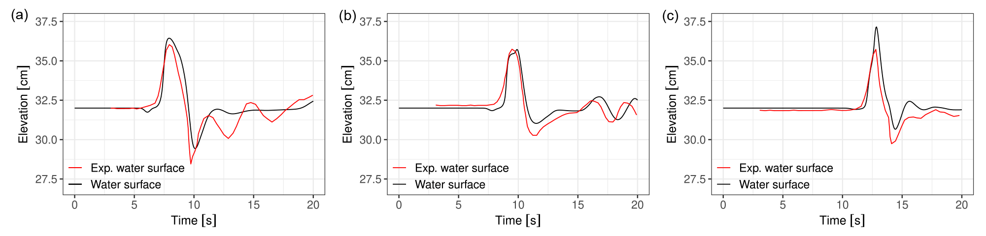
Figure 11 Simulated and experimental results of unsteady flow over an island for gauges G9 (a), G16 (b), and G22 (c).

5.2 Experimental unsteady flow over an island

Briggs et al. (1995) presented an experimental test of an unsteady flow over a conical island. This test has been extensively used for benchmarking (Bradford and Sanders, 2002; Choi et al., 2007; García-Navarro et al., 2019; Hou et al., 2013b; Liu et al., 1995; Lynett et al., 2002; Nikolos and Delis, 2009). A truncated cone of base diameter 7.2 m and top diameter 2.2 m and with a height of 0.625 m was placed at the centre of a 26 m × 27.6 m smooth and flat domain. An initial hydrostatic water level of h₀ = 0.32 m was set, and a wave was imposed on the boundary following

$$\begin{array}{}\text{(7)}& {\displaystyle }{h}_{\mathrm{b}}=h_{\mathrm{0}}+A{\mathrm{sech}}^{\mathrm{2}}\left({\displaystyle \frac{B(t-T)}{C}}\right),\text{(8)}& {\displaystyle }B=\sqrt{g{h}_{\mathrm{0}}}\left(\mathrm{1}+{\displaystyle \frac{A}{\mathrm{2}{h}_{\mathrm{0}}}}\right),\text{(9)}& {\displaystyle }C=h_{\mathrm{0}}\sqrt{{\displaystyle \frac{\mathrm{4}{h}_{\mathrm{0}}B}{\mathrm{3}A\sqrt{g{h}_{\mathrm{0}}}}}},\end{array}$$

where A = 0.032 m is the wave amplitude, and T = 2.84 s is the time at which the peak of the wave enters the domain. Figure 11 shows results for a simulation with a 2.5 cm resolution, resulting in 1.2 million cells. A roughness coefficient of 0.013 $\mathrm{s}{\mathrm{m}}^{-\mathrm{1}/\mathrm{3}}$ was used for the concrete surface. The results are comparable to previous solutions in the literature, in general reproducing well the water surface, with some delay over experimental measurements.

5.3 Experimental rainfall runoff over an idealised urban area

Cea et al. (2010a) presented experimental and numerical results for a range of laboratory-scale rainfall runoff experiments on an impervious surface with different arrangements of buildings, which have been frequently used for model validation (Caviedes-Voullième et al., 2020a; Cea et al., 2010b; Cea and Bladé, 2015; Fernández-Pato et al., 2016; Su et al., 2017; Xia et al., 2017). This laboratory-scale test includes non-trivial topographies, small water layers, and wetting–drying fronts, making it a good benchmark for realistic rainfall runoff conditions.

The dimensions of the experimental flume are 2 m × 2.5 m. Here, we select one building arrangement named A12 by Cea et al. (2010a). The original digital elevation model (DEM) is available (from Cea et al., 2010a) at a resolution of 1 cm. The buildings are 20 cm high and are represented as topographical features on the domain. All boundaries are closed, except for the free outflow at the outlet. The domain was discretised with a δx = 1 cm resolution, resulting in 54 600 cells. The domain was forced by two constant pulses of rain of 85 and 300 mm h⁻¹ (lowest and highest intensities in the experiments) with durations of 60 and 20 s. The simulation was run up to t = 200 s. Friction was modelled by Manning's equation, with a constant roughness coefficient of 0.010 $\mathrm{s}{\mathrm{m}}^{-\mathrm{1}/\mathrm{3}}$ for steel (Cea et al., 2010a).

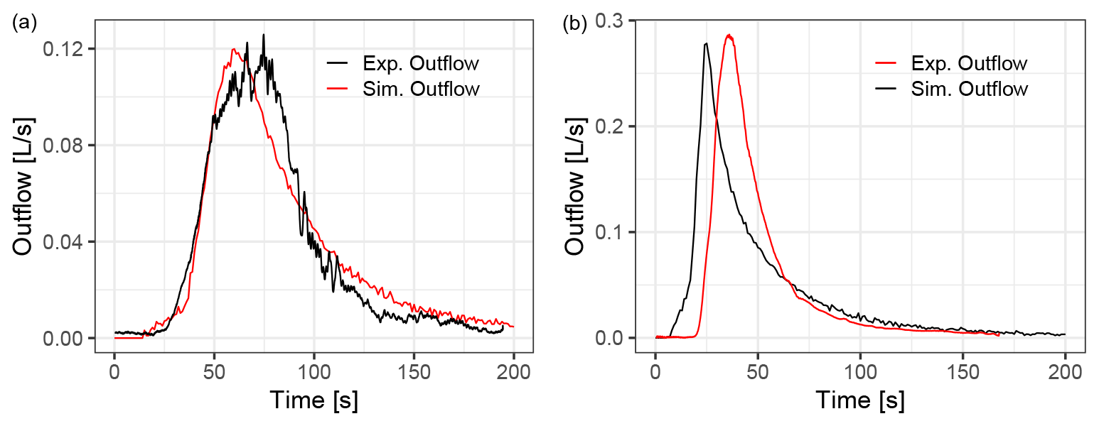
Figure 12 Simulated hydrographs compared to experimental data from Cea et al. (2010a) for two rainfall pulses on the A12 building arrangement. (a) Rain intensity 85 mm h⁻¹, duration 60 s. (b) Rain intensity 300 mm h⁻¹, duration 20 s

Figure 12 shows the experimental and simulated outflow discharge for both rainfall pulses. There is a very good qualitative agreement, and peak flow is quantitatively well reproduced by the simulations. For the 300 mm h⁻¹ intensity rainfall, the onset of runoff is earlier than in the experiments, and overall the hydrograph is shifted towards earlier times. Cea et al. (2010a) observed a similar behaviour and pointed out that this is likely caused by surface tension during the early wetting of the surface, and it was most noticeable on the experiments with higher rainfall intensity.

6 Plot-scale to catchment-scale experiments

6.1 Plot-scale field rainfall runoff experiment

Tatard et al. (2008) presented a rainfall runoff plot-scale experiment performed in Thiès, Senegal. This test has been used often for benchmarking of rainfall runoff models (Caviedes-Voullième et al., 2020a; Chang et al., 2016; Mügler et al., 2011; Özgen-Xian et al., 2020; Park et al., 2019; Simons et al., 2014; Yu and Duan, 2017; Weill, 2007). The domain is a field plot of 10 m × 4 m, with an average slope of 0.01. A rainfall simulation with an intensity of 70 mm h⁻¹ during 180 s was performed. Steady velocity measurements were taken at 62 locations. The Gauckler–Manning roughness coefficient was set to 0.02 $\mathrm{s}{\mathrm{m}}^{-\mathrm{1}/\mathrm{3}}$, and a constant infiltration rate was set to 0.0041667 mm s⁻¹ (Mügler et al., 2011). The domain was discretised with δx = 0.02666 m, resulting in 56 250 cells, with a single free-outflow boundary downslope.

Simulated velocities are compared to experimental velocities at the 62 gauged locations in Fig. 13. A good agreement between simulated and experimental velocities exists, especially in the lower-velocity range. The agreement is similar to previously reported results (e.g. Caviedes-Voullième et al., 2020a), and the differences between simulated and observed velocities have been shown to be a limitation of a depth-independent roughness and Manning's model (Mügler et al., 2011).

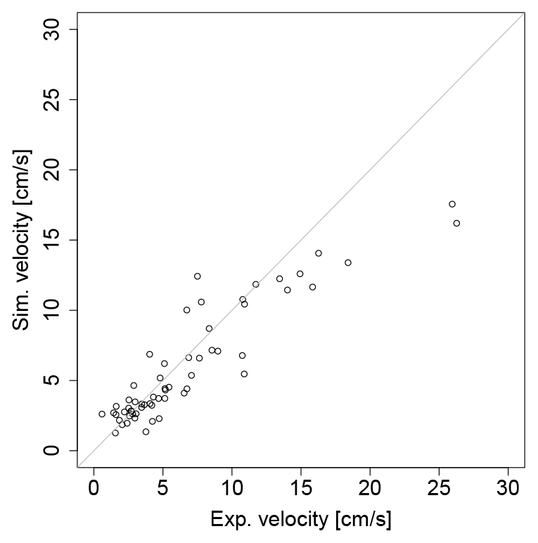
Figure 13 Comparison of simulated (line) and experimental (circles) steady velocities in the Thiès field case.

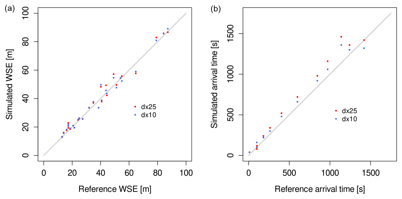
Figure 14 Water surface elevations (a) and arrival time (b) result comparison for two meshes of the Malpasset case.

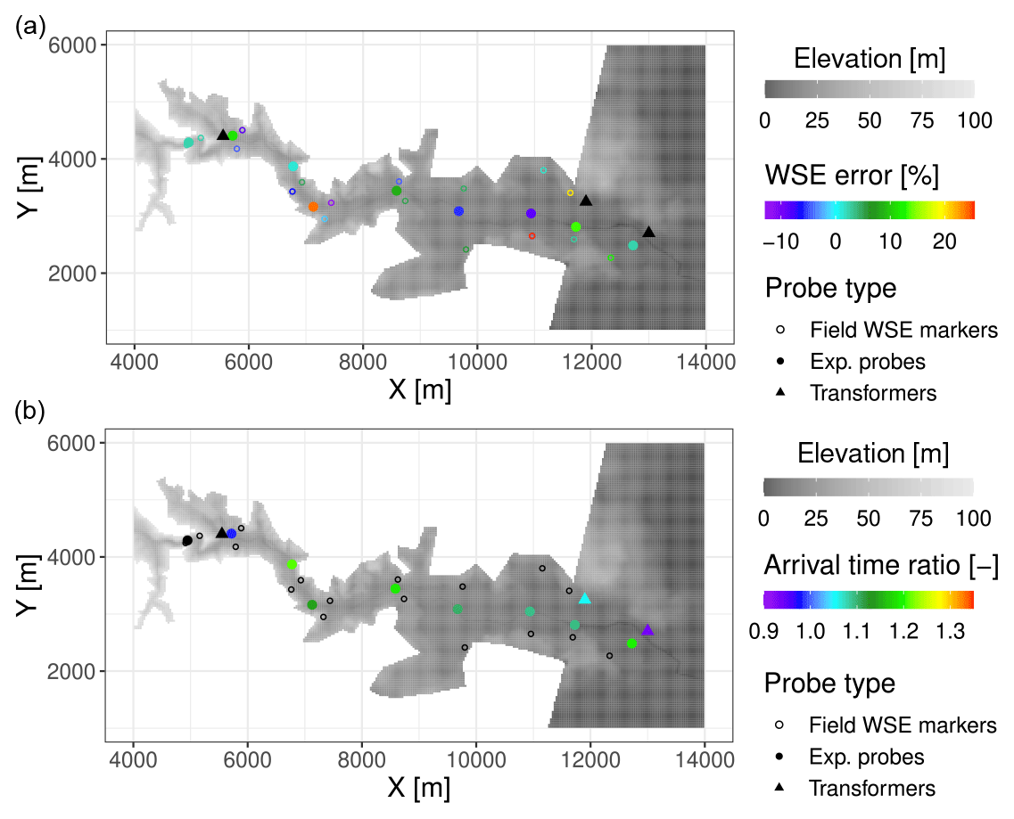
Figure 15 Geolocated relative WSE error (a) and ratio of arrival time (b) for the Malpasset dam break test case with δx = 10 m.

Table 4 HPC systems in which SERGHEI-SWE has been tested.

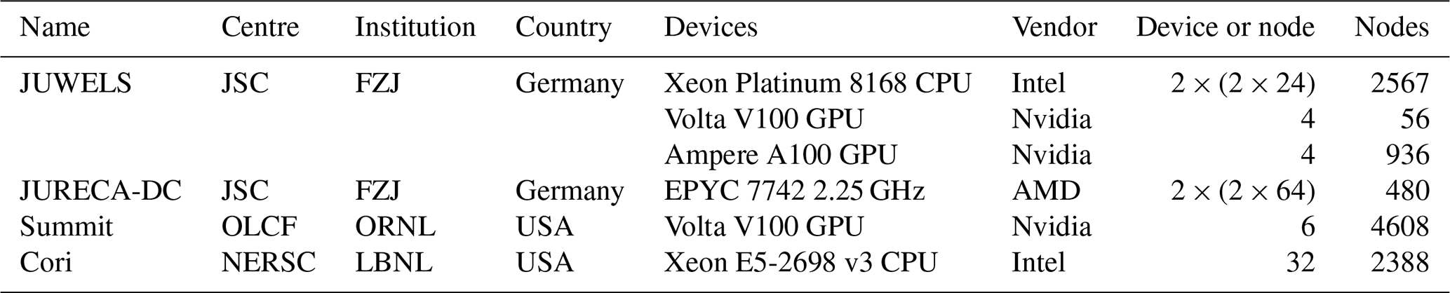
JSC: Jülich Supercomputing Centre; FZJ: Forschungszentrum Jülich; OLCF: Oak Ridge Leadership Computing Facility; ORNL: Oak Ridge National Laboratory; NERSC: National Energy Research Scientific Computing Center; LBNL: Lawrence Berkeley National Laboratory

6.2 Malpasset dam break

The Malpasset dam break event (Hervouet and Petitjean, 1999) is the most commonly used real-scale benchmark test in shallow-water modelling (An et al., 2015; Brodtkorb et al., 2012; Brufau et al., 2004; Caviedes-Voullième et al., 2020b; Duran et al., 2013; George, 2010; Hervouet and Petitjean, 1999; Hou et al., 2013a; Kesserwani and Liang, 2012; Kesserwani and Sharifian, 2020; Kim et al., 2014; Liang et al., 2007; Sætra et al., 2015; Schwanenberg and Harms, 2004; Smith and Liang, 2013; Valiani et al., 2002; Xia et al., 2011; Yu and Duan, 2012; Wang et al., 2011; Zhou et al., 2013; Zhao et al., 2019). Although it may not be particularly challenging for current solvers, it remains an interesting case due to its scale and the available field and experimental data (Aureli et al., 2021). The computational domain was discretised to δx = 25 m and δx = 10 m (resulting in 83 137 and 515 262 cells, respectively). The Gauckler–Manning coefficient was set to a uniform value of 0.033 $\mathrm{s}{\mathrm{m}}^{-\mathrm{1}/\mathrm{3}}$, which has been shown to be a good approximation in the literature. Figure 14 shows a comparison of simulated water surface elevation (WSE) and arrival time for two resolutions against the reference experimental and field data. Figure 15 shows the geospatial distribution of the relative WSE error and the ratio of the simulated arrival time to the observed time. Overall, WSE shows a good agreement and somewhat smaller scatter for the higher resolution. Arrival time tends to be overestimated, somewhat more for coarser resolutions.

7 Performance and scaling

In this section we report an investigation of the computational performance and parallel scaling of SERGHEI-SWE for selected test cases. To demonstrate performance portability, we show performance metrics for both OpenMP and CUDA backends enabled by Kokkos, computed on CPU and GPU architectures, respectively. For that, hybrid MPI-OpenMP and MPI-CUDA implementations are used, with one MPI task per node for MPI-OpenMP and one MPI task per GPU for MPI-CUDA. Most of the runs were performed on JUWELS at JSC (Jülich Supercomputing Centre). Additional HPC systems were also used for come cases. Properties of all systems are shown in Table 4. Additionally, we provide performance metrics on non-HPC systems, including some consumer-grade GPUs.

It is important to highlight that no performance tuning or optimisation has been carried out for these tests and that no system-specific porting efforts were done. All runs relied entirely on Kokkos for portability. The code was simply compiled with the available software stacks in the HPC systems and executed. All results reported here were computed using double-precision arithmetic.

7.1 Single-node scaling – Malpasset dam break

The commonly used Malpasset dam break test (introduced in Sect. 6.2) was also tested for computational performance at a resolution of δx = 10 m. Results are shown in Fig. 16. The case was computed on CPUs, a single JUWELS node, and a single JURECA-DC node. Three additional runs with single Nvidia GPUs were carried out: a commercial-grade GeForce RTX 3070, 8 GB GPU (in a desktop computer), and two scientific-grade cards V100 and A100, respectively (in JUWELS). As Fig. 16 shows, CPU runtime quickly approaches an asymptotic behaviour (therefore demonstrating that additional nodes are not useful in this case). Notably, all three GPUs outperform a single CPU node, and the performance gradient among the GPUs is evident. The A100 GPU is roughly 6.5 faster than a full JUWELS CPU node, and even for the consumer-grade RTX 3070, the speed-up compared to a single HPC node is 2.2. Although it is possible to scale up this case with significantly higher resolution and test it with multiple GPUs, it is not a case well suited to such a scaling test. Multiple GPUs (as well as multiple nodes with either CPUs or GPUs) require a domain decomposition. The orientation of the Malpasset domain is roughly NW–SE, which makes both 1D decompositions (along x or y) and 2D decompositions (x and y) inefficient, as many regions have no computational load. Moreover, the dam break nature of the case implies that a large part of the valley is dry for long periods of time; therefore, load balancing among the different nodes and/or GPUs will be poor.

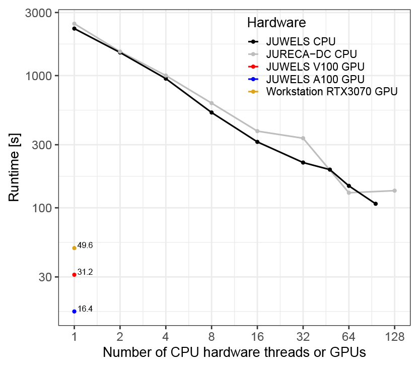
Figure 16 Scaling for the Malpasset case (δx = 10 m) on a single node and on single GPUs. GPU speed ups relative to a full JUWELS node are 6.5 (A100), 3.4 (V100), and 2.2 (RTX 3070).

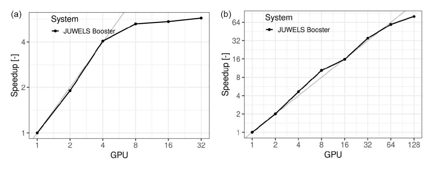
Figure 17 Strong scaling behaviour for a circular dam break test case with two resolutions. (a) δx = 0.05, 64 million cells. (b) δx=0.025, 256 million cells.

Figure 18 Runtime (a) and speed up (b) for a strong-scaling experiment with SERGHEI-SWE using CPUs on Cori and JUWELS for the short rainfall event. See Table 4 for details on the systems.

7.2 HPC scaling – 2D circular dam break case

This is a simple analytical verification test in the shallow-water literature, which generalises the 1D dam break solution. We purposely select this case (instead of one of the many verification problems) for its convenience for scaling studies. Firstly, resolution can be increased at will. Additionally, the square domain allows for trivial domain decomposition, which together with the fully wet domain and the radially symmetric flow field minimises load-balancing issues. Essentially, it allows for a very clean scalability test with minimal interference from the problem topology, which facilitates scalability and performance analysis (in contrast to the limitations of the Malpasset domain discussed in Sect. 7.1). We take a 400 m × 400 m flat domain with the centre at (0,0) and initial conditions given by

$$\begin{array}{}\text{(10)}& h(x,y,t=\mathrm{0})=\left\{\begin{array}{ll}\mathrm{4}& \text{if }\sqrt{x^{\mathrm{2}}+y^{\mathrm{2}}}\le \mathrm{50}\\ \mathrm{1}& \text{otherwise}.\end{array}\right.\end{array}$$

We generated three computational grids, with δx = 0.05, 0.025, 0.0175 m, which correspond to 64, 256, and 552 million cells, respectively. Figure 17 shows the strong-scaling results for the 64 and 256 million cells cases, computed in the JUWELS-booster system, on A100 Nvidia GPUs. The 64 million does not scale well beyond 4 GPUs. However, the 256-million-cells problem scales well up to 64 GPUs (and efficiency starts to decrease with 128), showing that the first case simply is too small for significant gains.

For the 552-million-cells grid, only two runs were computed with 128 and 160 GPUs (corresponding to 32 and 40 nodes in JUWELS-booster, respectively). Runtime for these was 95.4 and 84.7 s, respectively, implying a very good 89 % scaling efficiency for this large number of GPUs. For this problem and these resources, the time required for inter-GPU communications is comparable to that used by kernels computing fluxes and updating cells, signalling scalability limits for this case on the current implementation.

Figure 19 Runtime (a) and speed up (b) for a strong-scaling experiment with SERGHEI-SWE using GPUs on Summit and JUWELS for the long rainfall event. See Table 4 for details on the systems.

7.3 HPC scaling of rainfall runoff in a large catchment

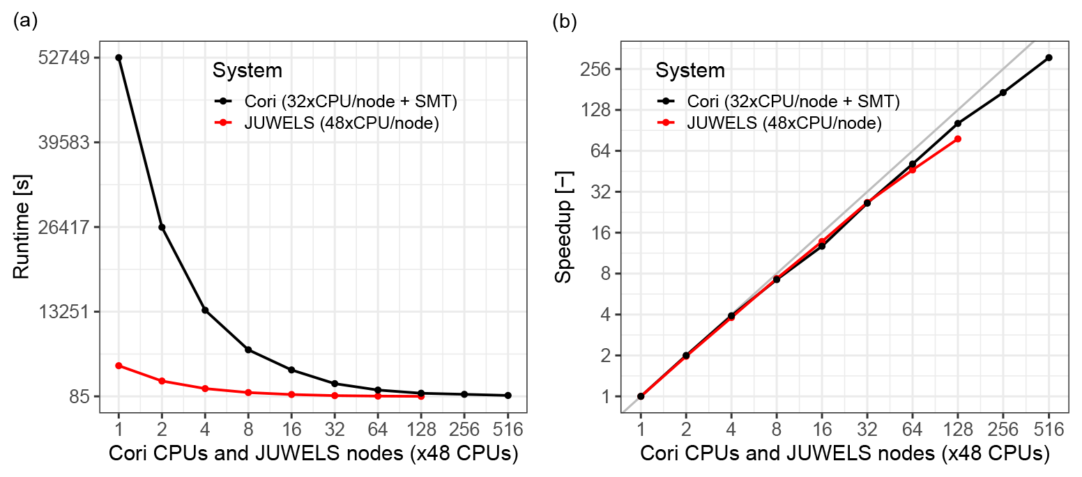
To demonstrate scaling under production conditions of real scenarios, we use an idealised rainfall runoff simulation over the Lower Triangle region in the East River Watershed (Colorado, USA) (Carroll et al., 2018; Hubbard et al., 2018; Özgen-Xian et al., 2020). The domain has an area of 14.82 km² and elevations ranging from 2759–3787 m. The computational problem is defined with a resolution of δx = 0.5 m (matching the highest-resolution DEM available), resulting in 122 × 10⁶ computational cells. Although this is not a particularly large catchment, the very-high-resolution DEM available makes it an interesting performance benchmark, which is our sole interest in this paper.

For practical purposes, two configurations have been used for this test: a short rainfall of T = 870 s, which was computed in Cori and JUWELS to assess CPU performance and scalability (results shown in Fig. 18), and a long rainfall event lasting T = 12 000 s, which was simulated in Summit and JUWELS to assess GPU performance and scalability, with results shown in Fig. 19. CPU results (Fig. 18) show that the strong scaling behaviour in Cori and JUWELS is very similar. Absolute runtimes are longer for Cori, since the scaling study was carried out starting from a single core, whereas in JUWELS it was with a full node (i.e. 48 cores). Most importantly, the GPU strong-scaling behaviour overlaps almost completely between JUWELS and Summit, although computations in Summit were somewhat faster. CPU and GPU scaling are clearly highly efficient, with similar behaviour. These results demonstrate the performance portability delivered via Kokkos to SERGHEI.

8 Conclusions and outlook

In this paper we present the SERGHEI framework and, in particular, the SERGHEI-SWE module. SERGHEI-SWE implements a 2D fully dynamic shallow-water solver, harnessing state-of-the-art numerics and leveraging on Kokkos to facilitate portability across architectures. We show through empirical evidence with a large set of well-established benchmarks that SERGHEI-SWE is accurate, numerically stable, and robust. Importantly, we show that SERGHEI-SWE's parallel scaling is very good for CPU-based HPC systems, consumer-grade GPUs, and GPU-based HPC systems. Consequently, we claim that SERGHEI is indeed performance portable and approaching exascale readiness. These features make SERGHEI-SWE a plausible community code for shallow-water modelling for a wide range of applications requiring large-scale, very-high-resolution simulations.

Exploiting increasingly better and highly resolved geospatial information (DEMs, land use, vector data of structures) prompts the need for high-resolution solvers. At the same time, the push towards the study of multiscale systems and integrated management warrants increasingly larger domains. Together, these trends result in larger computational problems, motivating the need for exascale-ready shallow-water solvers. Additionally, HPC technology is evermore available, not only via (inter)national research facilities but also through cloud-computing facilities. It is arguably timely to enable such an HPC-ready solver.

The HPC allows for not only large simulations but also large ensembles of simulations, allowing uncertainty issues to be addressed and enabling scenario analysis for engineering problems, parameter space exploration, and hypothesis testing. Furthermore, although the benefits of high resolution may be marginal for runoff hydrograph estimations, they allow the local dynamics to be better resolved in the domain. Flow paths, transit times, wetting–drying dynamics, and connectivity play important roles in transport and ecohydrological processes. For these purposes, enabling very-high-resolution simulations will prove to be highly beneficial. We also envision that, provided with sufficient computational resources, SERGHEI-SWE could be used for operational flood forecasting and probabilistic flash-flood modelling. Altogether, this strongly paves the way for the uptake of shallow-water solvers by the broader ESM community and its coupling to Earth system models, as well as their many applications, from process and system understanding to hydrometeorological risk and impact assessment. We also envision that, for users not requiring HPC capabilities, the benefit of SERGHEI-SWE is access to a transparent, open-sourced, performance-portable software that allows workstation GPUs to be exploited efficiently.

As additional SERGHEI modules become operational, the HPC capabilities will further enable simulations that are unfeasible with the current generation of available solvers. For example, with a fully operational transport and morphology module, it will be possible to run decade-long morphological simulations relevant for river management applications; to better capture sediment connectivity and sediment cascades across the landscape, a relevant topic for erosion and catchment management; or to perform catchment-scale hydro-biogeochemical simulations with unprecedented high spatial resolutions for better understanding of ecohydrological and biogeochemical processes.

Finally, SERGHEI is conceptualised and designed with extendibility and software interoperability in mind, with design choices made to facilitate foreseeable future developments on a wide range of topics, such as

1. numerics, e.g. the discontinuous Galerkin discretisation strategies (Caviedes-Voullième and Kesserwani, 2015; Shaw et al., 2021) and multiresolution adaptive meshing (Caviedes-Voullième et al., 2020b; Kesserwani and Sharifian, 2020, 2022; Özgen-Xian et al., 2020);

2. interfaces to mature geochemistry engines, e.g. CrunchFlow (Steefel, 2009) and PFLOTRAN (Lichtner et al., 2015);

3. vegetation models with varying degrees of complexity, for example, Ecosys (e.g. Grant et al., 2007; Grant and the Ecosys development team, 2022) and EcH2O (Maneta and Silverman, 2013).

Appendix A: Additional validation test cases

This appendix contains an extended set of relevant test cases that are commonly used as validation cases in the literature. It complements and extends the verification evidence in Sect. 4.

A1 C property: immersed bump

Using the same set-up as in Sect. 4.1.1, but with a higher water surface elevation, in Fig. A1 we demonstrate how SERGHEI-SWE also conserves the C property for an immersed bump.

Figure A1 Lake-at-rest solution for an immersed bump.

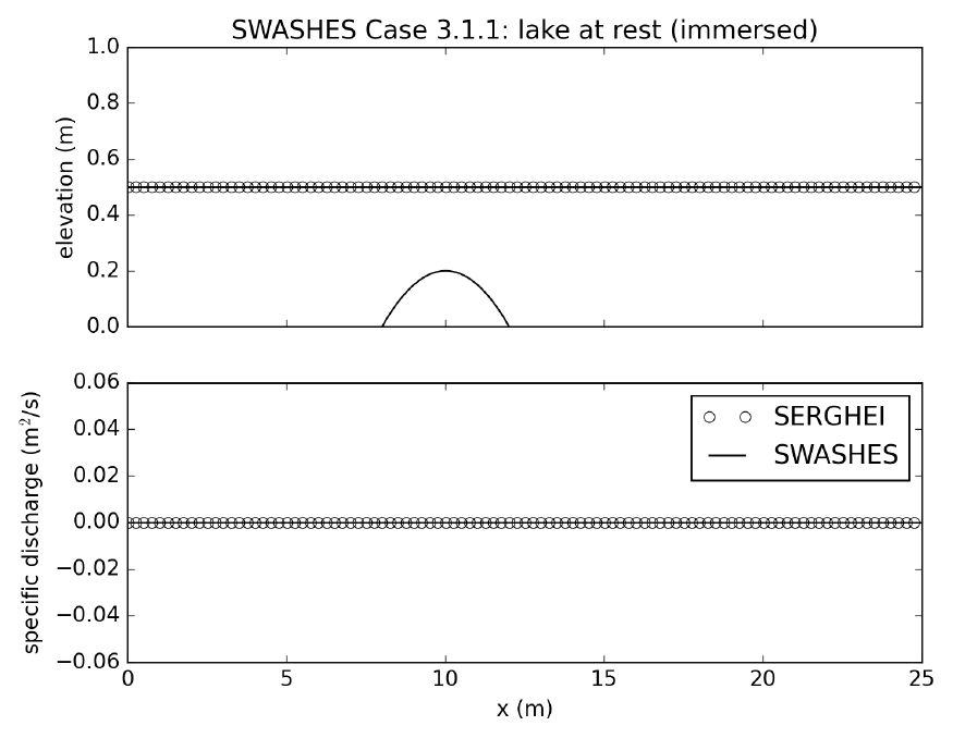
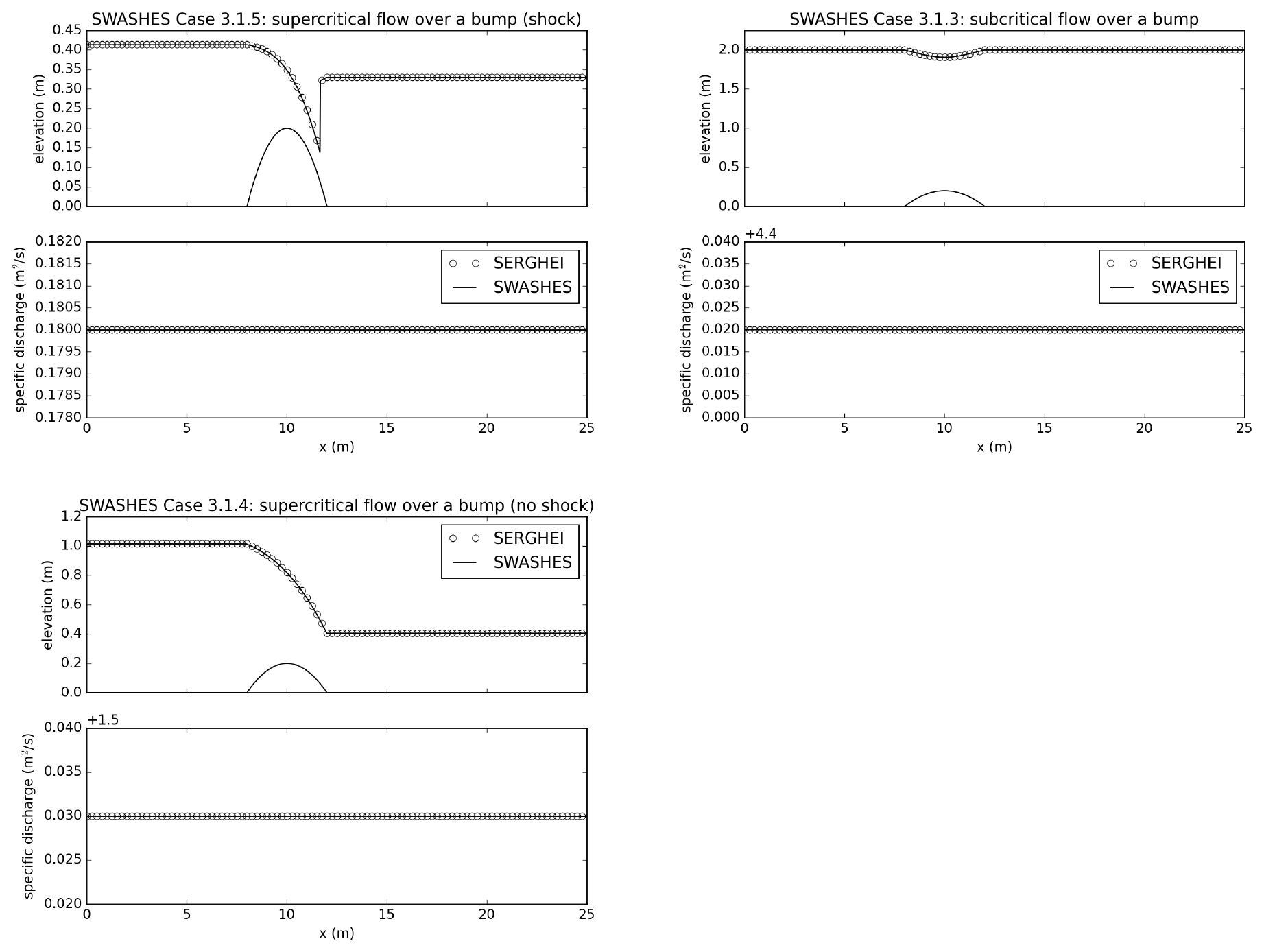
Figure A2 Analytical steady flows over a bump. SERGHEI-SWE captures moving equilibria solutions for transcritical flow with a shock (top left), fully subcritical flow (top right), and transcritical flow without a shock (bottom)

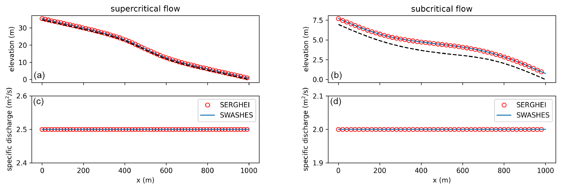
Figure A3 Analytical steady flows: flumes. SERGHEI-SWE captures moving equilibria solutions for a subcritical (a, c) and supercritical (b, d) flow. Note that the solution is stable (no oscillations) and well-balanced (discharge remains constant along the flume).

A2 Well-balancing

To further show that SERGHEI-SWE is well-balanced, we computed three steady flows over a bump. We include a transcritical flow with a shock wave, a fully subcritical flow, and a transcritical flow, as shown in Fig. A2. All of SERGHEI-SWE predictions show excellent agreement with the analytical solution. The constant unit discharge is captured with machine accuracy without oscillations at the shock, which is an inherent feature of the augmented Roe solver (Murillo and García-Navarro, 2010).

We also include two additional cases from MacDonald et al. (1995) for fully supercritical and subcritical flows in Fig. A3. These results and their L norms in Table A1 further confirm well-balancing.

Additionally, MacDonald-type solutions can be constructed for frictionless flumes to study the bed slope source term implementation in isolation. We present a frictionless test case with SERGHEI-SWE that is not part of the SWASHES benchmark compilation. We discretise the bed elevation of the flume as

$$\begin{array}{}\text{(A1)}& z\left(x\right)=C_{\mathrm{0}}-{\displaystyle \frac{\mathrm{1}}{\mathrm{2}}}\exp (-\mathrm{0.001}x)-{\displaystyle \frac{\mathrm{2}{q}_{\mathrm{0}}^{\mathrm{2}}\exp \left(\mathrm{0.002}x\right)}{g}},\end{array}$$

where C₀ is an arbitrary integration constant and q₀ is a specified unit discharge. The water depth for this topography is

$$\begin{array}{}\text{(A2)}& h\left(x\right)={\displaystyle \frac{\mathrm{1}}{\mathrm{2}}}\exp (-\mathrm{0.001}x).\end{array}$$

Using C₀ = 1.0 m and q₀ = 1.0 m² s⁻¹, we obtain the solution plotted in Fig. A4. SERGHEI-SWE's prediction and the analytical solution show good agreement.

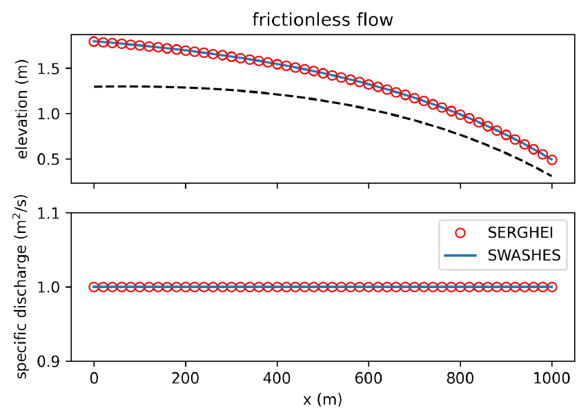
Figure A4 Analytical steady flows: flumes. SERGHEI-SWE captures moving equilibrium solution for frictionless test case, with a stable and well-balanced solution.

L norms for errors in water depth are summarised in Table A1 for the sake of completeness. L norms of a vector x with length N and entries x_i, where $i\in [\mathrm{0},N)\subset {\mathbb{Z}}^{+}$ is the index of the entries, are calculated as

$$\begin{array}{}\text{(A3)}& L_{\langle n\rangle }={\left(\sum _i^N|x_i{|}^{\langle n\rangle }\right)}^{\frac{\mathrm{1}}{\langle n\rangle }},\end{array}$$

with $\langle n\rangle \in {\mathbb{Z}}^{+}$ being the order of the L norm. The L_∞ norm is calculated as

$$\begin{array}{}\text{(A4)}& L_{\mathrm{\infty }}=max\mathrm{|}{x}_i\mathrm{|},x_i\in \mathbf{x}.\end{array}$$

The L norms for errors in unit discharge are in the range of machine accuracy for all cases and are omitted here.

Table A1 Analytical steady flows: summary of L norms for errors in water depth; L norms for errors in unit discharge are in the range of machine accuracy and are omitted here.

A3 Dam break over a wet bed without friction

The dam break on a wet-bed-without-friction test case is configured by setting water depths in the domain as h_L = 0.005 m and h_R = 0.001 m. The domain is 10 m long, and the discontinuity is located at x₀ = 5 m. The total run time is 6 s. Figure A5 shows the model results obtained on successively refined grids compared against the analytical solution by Stoker (1957). Errors for this test case are reported in Table A2. We also report the observed convergence rate qR, calculated on the basis of the L₁ norm. As the grid is refined, the model result converges to the analytical solution. Due to the discontinuities in the solution, the observed convergence rate is below the theoretical convergence rate of R=1.

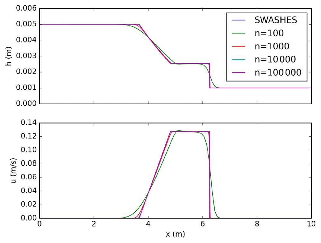
Figure A5 Dam break on wet bed without friction: model predictions for different number of grid cells. SERGHEI-SWE converges to the analytical solution (Stoker's solution) as the grid is refined.

Table A2 Analytical dam break: L norms and empirical convergence rates (R) for water depth (h) and velocity (u).

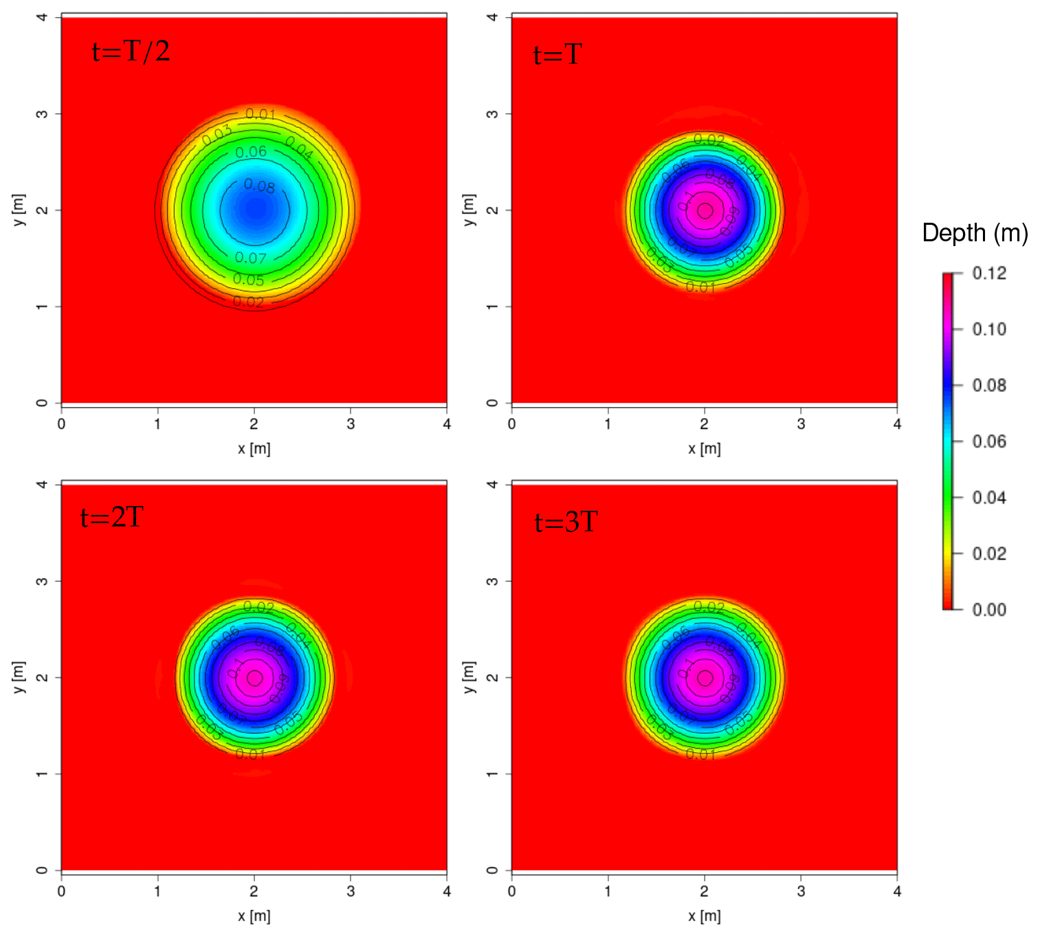
Figure A6 Radially symmetrical paraboloid: snapshots of water depth by the model compared to the analytical solution (contour lines). Period T = 2.242851 s.

A4 Radially symmetrical paraboloid

Using the same computational domain and bed topography as the case in Sect. 4.3, results for the radially symmetrical oscillation in a frictionless paraboloid (Thacker, 1981) are presented here. The details about the initial condition and the analytical solution for the water depth and velocities can be found in Delestre et al. (2013). In particular, the analytical solution at t = 0 s is set as the initial condition, and three periods are simulated using δx = 0.01 m as the grid resolution. Figure A6 shows the numerical and analytical solution at four different times. Although the analytical solution is periodic without dumping, the numerical results show a diffusive behaviour attributed to the numerical diffusion introduced by the first-order scheme. Other than that, model results show good agreement with the analytical solution.

Figure A7 Simulated and experimental results for the laboratory-scale tsunami case at gauges G1 (a), G2 (b), and G3 (ca).

Figure A8 Simulated (black lines) and experimental (red points) transient water depths at seven gauge points (x = 17.5, x = 19.5, x = 23.5, x = 25.5, x = 26.5, x = 28.5, x = 35.5, from a to b) for the dam break over a triangular sill.

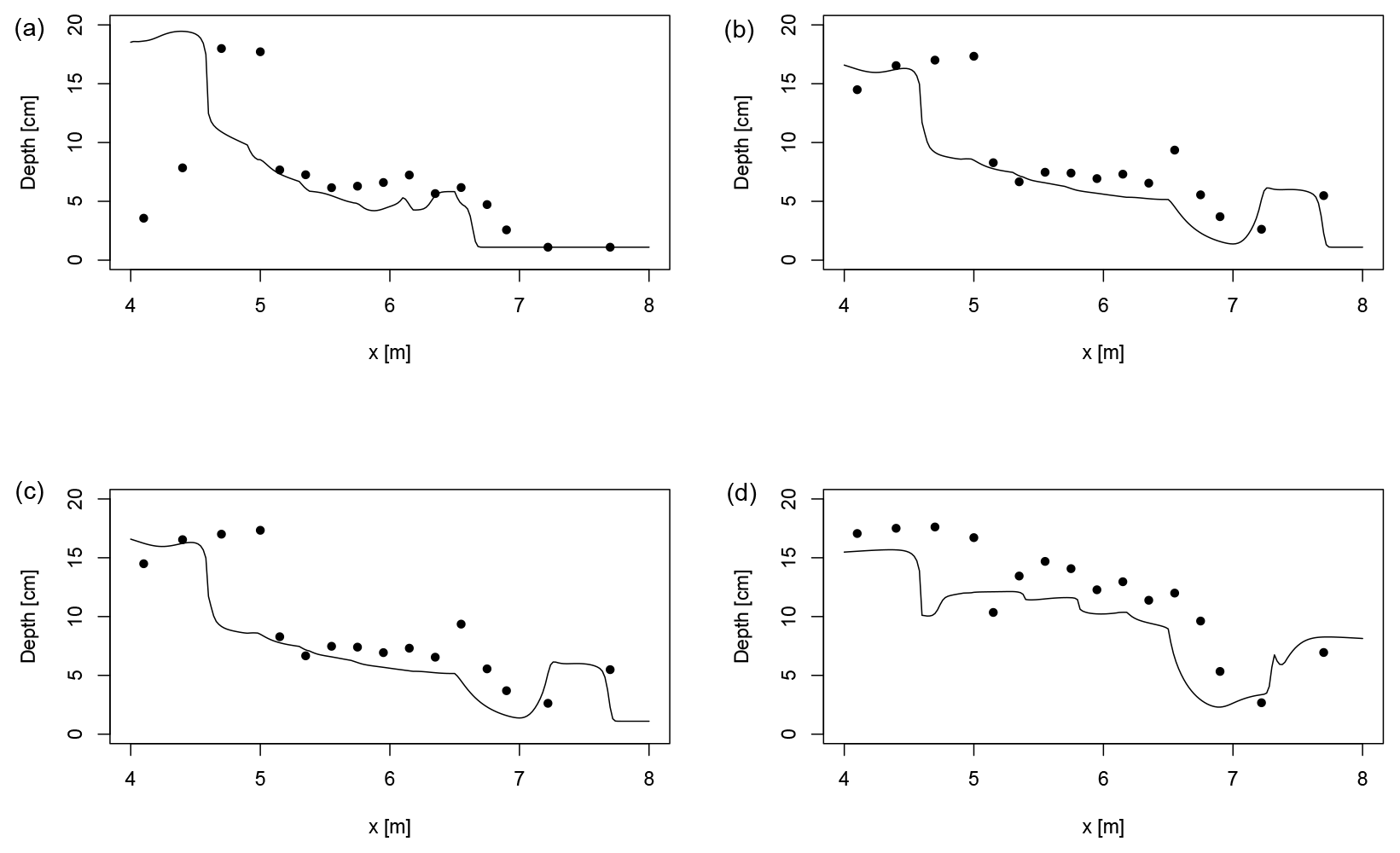
Figure A9 Simulated (lines) and experimental (points) water depth profiles at y = 0.2 m, at four times (4, 5, 6 and 10 s, a to d) for the idealised urban dam break case.

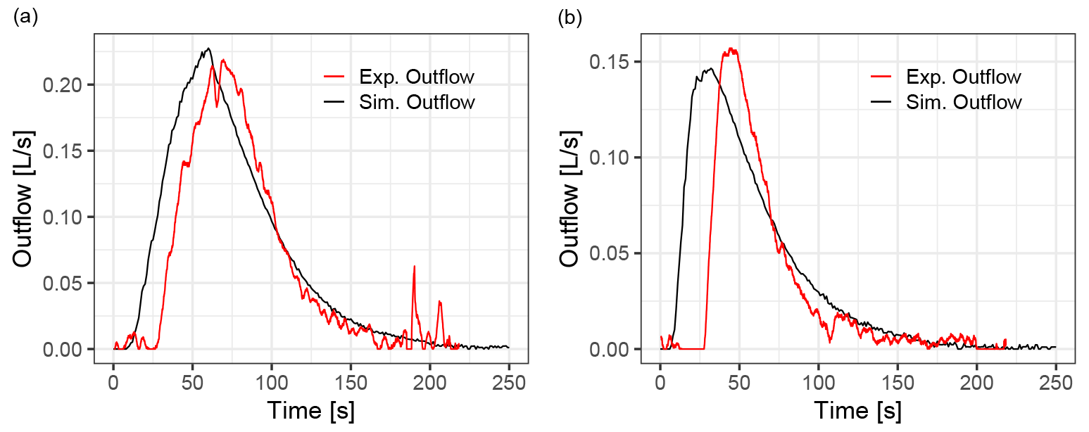
Figure A10 Simulated hydrographs compared to experimental data from Cea et al. (2010b) for two rainfall pulses on the L180 building arrangement. (a) Rainfall intensity 180 mm h⁻¹, duration 60 s. (b) Rainfall intensity 300 mm h⁻¹, duration 20 s.

A5 Experimental laboratory-scale tsunami

A 1:400-scale experiment of a tsunami run-up over the Monai valley (Japan) was reported by Matsuyama and Tanaka (2001); The third international workshop on long-wave runup models (2004), providing experimental data on the temporal evolution of the water surface at three locations and of the maximum run-up. A laboratory basin of 2.05 m × 3.4 m was used to create a physical scale model of the Monai coastline. A tsunami was simulated by appropriate forcing of the boundary conditions. This experiment has been extensively used to benchmark SWE solvers (Arpaia and Ricchiuto, 2018; Caviedes-Voullième et al., 2020b; Hou et al., 2015, 2018; Kesserwani and Liang, 2012; Kesserwani and Sharifian, 2020; Morales-Hernández et al., 2014; Murillo et al., 2009; Murillo and García-Navarro, 2012; Nikolos and Delis, 2009; Serrano-Pacheco et al., 2009; Vater et al., 2019). The domain was discretised with a resolution of 1.4 cm, producing 95 892 elements. Simulated water surface elevations are shown together with the experimental measurements in Fig. A7 at three gauge locations. The results agree well with experimental measurements, both in the water surface elevations and the arrival times of the waves.

A6 Experimental dam break over a triangular sill

Hiver (2000) presented a large flume experiment of a dam break over a triangular sill, which is a standard benchmark in dam break problems (Caviedes-Voullième and Kesserwani, 2015; Bruwier et al., 2016; Kesserwani and Liang, 2010; Loukili and Soulaïmani, 2007; Murillo and García-Navarro, 2012; Yu and Duan, 2017; Zhou et al., 2013), together with the reduced-scale version (Soares-Frazāo, 2007; Hou et al., 2013a, b; Yu and Duan, 2017).

The computational domain was discretised with a 380 × 5 grid, with a δx = 0.1 m resolution. Figure A8 shows simulated and experimental results for the triangular sill case. A very good agreement can be observed, both in terms of peak depths occurring whenever the shock wave passes through a gauge and in the timing of the shock wave movement. The simulations tend to slightly overestimate the peaks of the shock wave, as well as to overestimate the waves downstream of the sill (see plot for gauge at x = 35.5 m). Both behaviours are well documented in the literature.

A7 Experimental idealised urban dam break

A laboratory-scale experiment of a dam break over an idealised urban area was reported by Soares-Frazāo and Zech (2008) in a concrete channel including 25 obstacles representing buildings separated by 10 cm. It is widely used in the shallow-water community (Abderrezzak et al., 2008; Caviedes-Voullième et al., 2020b; Ginting, 2019; Hartanto et al., 2011; Jeong et al., 2012; Özgen et al., 2015a; Petaccia et al., 2010; Wang et al., 2017) because of its fundamental phenomenological interest and because it is demanding in terms of numerical stability and model performance. The small buildings and streets in the geometry require sufficiently high resolutions, both to capture the geometry and to capture the complex flow phenomena which are triggered in the streets. Experimental measurements of transient water depth exist at different locations, including in between the buildings. A resolution of 2 cm was used for the simulated results in Fig. A9, together with experimental data. The results agree well with the experimental observations to a similar degree as to what has been reported in the literature.

A8 Experimental rainfall runoff over a dense idealised urban area

Cea et al. (2010b) presented a laboratory-scale experiment in a flume with a dense idealised urban area. The case elaborates on the set-up of Cea et al. (2010a) (Sect. 5.3), including 180 buildings (case L180) in contrast to the 12 buildings in Sect. 5.3, which potentially requires a higher resolution to resolve the building (6.2 cm sides) and street width (∼ 2 cm) and the flow in the streets. We keep a 1 cm resolution. Rainfall is a single pulse of constant intensity. Two set-ups were used with intensities 180 and 300 mm h⁻¹ and durations of 60 and 20 s, respectively. As Fig. A10 shows, the hydrographs are well captured by the simulation, albeit with a delay. Analogously to Sect. 5.3, this can be attributed to surface tension in the early wetting phase.

Appendix B: Glossary

CFL	Courant–Friedrichs–Lewy
Cori	Cori supercomputer at the National Energy Research Scientific Computing Center (USA)
CPU	Central processing unit
CUDA	Compute Unified Device Architecture, programming interface for Nvidia GPUs
El Capitan	El Capitan supercomputer at the Lawrence Livermore National Laboratory (USA)
ESM	Earth system modelling
Frontier	Frontier supercomputer at the Oak Ridge Leadership Computing Facility (USA)
GPU	Graphics processing unit
HIP	Heterogeneous Interface for Portability, programming interface for AMD GPUs
HPC	High-performance computing
JURECA-DC	Data Centric module of the Jülich Research on Exascale Cluster Architectures supercomputer at the Jülich Supercomputing Centre (Germany)
JUWELS	Jülich Wizard for European Leadership Science, supercomputer at the Jülich Supercomputing Centre (Germany)
JUWELS-booster	Booster module of the JUWELS supercomputer (Germany)
Kokkos	Kokkos, a C++ performance portability layer
LUMI	LUMI supercomputer at CSC (Finland)
OpenMP	Open MultiProcessing, shared-memory programming interface for parallel computing
MPI	Message Passing Interface for parallel computing
SERGHEI	Simulation EnviRonment for Geomorphology, Hydrodynamics, and Ecohydrology in Integrated form
SERGHEI-SWE	SERGHEI's shallow-water equations solver
Summit	Summit supercomputer at the Oak Ridge Leadership Computing Facility (USA)
SWE	Shallow-water equations
SYCL	A programming model for hardware accelerators
UVM	Unified Virtual Memory
WSE	Water surface elevation