the Creative Commons Attribution 4.0 License.
the Creative Commons Attribution 4.0 License.
 | 07 Feb 2023
Massively parallel modeling and inversion of electrical resistivity tomography data using PFLOTRAN
Piyoosh Jaysaval
Glenn E. Hammond
Timothy C. Johnson
Electrical resistivity tomography (ERT) is a broadly accepted geophysical method for subsurface investigations. Interpretation of field ERT data usually requires the application of computationally intensive forward modeling and inversion algorithms. For large-scale ERT data, the efficiency of these algorithms depends on the robustness, accuracy, and scalability on high-performance computing resources. In this regard, we present a robust and highly scalable implementation of forward modeling and inversion algorithms for ERT data. The implementation is publicly available and developed within the framework of PFLOTRAN, an open-source, state-of-the-art massively parallel subsurface flow and transport simulation code. The forward modeling is based on a finite-volume discretization of the governing differential equations, and the inversion uses a Gauss–Newton optimization scheme. To evaluate the accuracy of the forward modeling, two examples are first presented by considering layered (1D) and 3D earth conductivity models. The computed numerical results show good agreement with the analytical solutions for the layered earth model and results from a well-established code for the 3D model. Inversion of ERT data, simulated for a 3D model, is then performed to demonstrate the inversion capability by recovering the conductivity of the model. To demonstrate the parallel performance of PFLOTRAN's ERT process model and inversion capabilities, large-scale scalability tests are performed by using up to 131 072 processes on a leadership class supercomputer. These tests are performed for the two most computationally intensive steps of the ERT inversion: forward modeling and Jacobian computation. For the forward modeling, we consider models with up to 122 ×106 degrees of freedom (DOFs) in the resulting system of linear equations and demonstrate that the code exhibits almost linear scalability on up to 10 000 DOFs per process. On the other hand, the code shows superlinear scalability for the Jacobian computation, mainly because all computations are fairly evenly distributed over each process with no parallel communication.
- Article
(3398 KB) - Full-text XML
- BibTeX
- EndNote


Direct current electrical resistivity tomography (ERT) is one of the key geophysical methods for shallow-subsurface investigations, having applications in areas such as groundwater (Dahlin, 2001; Johnson et al., 2012; Meyerhoff et al., 2014; Park et al., 2016; Greggio et al., 2018; Alshehri and Abdelrahman, 2021), mineral exploration (Badmus and Olatinsu, 2009; Bery et al., 2012; Uhlemann et al., 2018; Martínez et al., 2019), environmental monitoring and remediation (Rosales et al., 2012; Rucker et al., 2013; Gabarrón et al., 2020; Rockhold et al., 2020; Kessouri et al., 2022), and engineering problems (Dahlin, 1996; Rizzo et al., 2004; Lysdahl et al., 2017). It can also be used for large-scale deep-subsurface investigations, e.g., for geothermal systems, active volcano imaging, and tectonic studies (Storz et al., 2000; Caputo et al., 2003; Johnson et al., 2010; Richards et al., 2010). Additional applications can also be found in detailed reviews by Slater (2007), Revil et al. (2012), Loke et al. (2013), Singha et al. (2022), and the references therein. In recent years, availability of multi-electrode and multichannel instrumentations permitted the acquisition of massive amounts of ERT data consisting of tens of thousands or even hundreds of thousands of observations. Efficient inversion and interpretation of such massive datasets requires fast, accurate, and highly scalable forward modeling and inversion algorithms to simulate and invert ERT data in arbitrary 3D conductivity structures. This paper presents an open-source implementation of such ERT modeling and inversion algorithms.
ERT data simulation is performed by solving the electrostatic Poisson equation. Numerical methods are needed to solve the governing equation in arbitrary 3D conductivity structures. The most used numerical methods for 3D ERT modeling are the finite-difference (FD) method (Dey and Morrison, 1979; Spitzer, 1995; Penz et al., 2013), finite-element (FE) method (Coggon, 1971; Li and Spitzer, 2002; Rücker et al., 2006; Blome et al., 2009; Johnson et al., 2010; Ren et al., 2018), and integral equation method (Lee, 1975; Schulz, 1985; Méndez-Delgado et al., 1999). Among these methods, the FD and FE methods are attractive choices for highly heterogeneous distributions of electrical conductivity in the subsurface. However, application of the FD method is mostly limited to simple model geometries due to its requirement of Cartesian grids (Rücker et al., 2006). By contrast, the FE method has proven to be effective in accounting for complex geometries, specifically by using unstructured meshes (Rücker et al., 2006; Blome et al., 2009; Johnson et al., 2010; Ren et al., 2018).
The finite-volume (FV) method can also be used effectively to account for complex geometries (Jahandari and Farquharson, 2014). The FV method is usually seen relatively close to the FD method as it inherits the simplicity similar to the FD method in its implementation. Unlike the FD method which discretizes the differential form of the governing equation, the FV method, however, directly discretizes its integral form. Nevertheless, the FV method has rarely been considered for ERT simulation problems. In our literature search, we came across only Cockett et al. (2015), which implements the method for the ERT modeling.
On the other hand, ERT data inversion is a nonlinear optimization problem to minimize a cost function that represents a measure of the difference between observed and simulated ERT data. For large-scale 3D ERT data, the inversion is often performed iteratively by linearizing the optimization problem at each iteration, calculating a model update, updating a conductivity model, and subsequently simulating ERT data for the updated model to examine the new cost function. The process continues until the cost function reduces to a predefined tolerance level. The model update is typically calculated using a gradient-based local optimization method, e.g., the steepest-descent, conjugate-gradient, or the Gauss–Newton method (Park and Van, 1991; Ellis and Oldenburg, 1994; Zhdanov and Keller, 1994; Zhang et al., 1995; Günther et al., 2006; Johnson et al., 2010). The Gauss–Newton method has usually been preferred due to its high convergence rate. Indeed, the fast convergence occurs at the cost of intensive computations because the method requires building the Jacobian (or sensitivity) and/or Hessian matrices at each inversion iteration (Nocedal and Wright, 2006).
For large-scale 3D ERT problems with tens of millions of degrees of freedom (DOFs), forward modeling and inversion are computationally demanding jobs and may need hours, if not days, of computing time if the underlying algorithms are not properly implemented to scale well on high-performance computing (HPC) resources or supercomputers. For such datasets, it is computationally infeasible to use desktop-based ERT data processing software without exploiting HPC resources. Recently, a few open-source 3D ERT modeling and inversion codes have been developed to handle moderately sized ERT problems composed of up to a few million DOFs, e.g., ResIPy (Blanchy et al., 2020), SimPEG (Cockett et al., 2015), and pyGIMLI (Rücker et al., 2017). However, these codes still lack full-scale parallel implementations to efficiently distribute computations over a supercomputer. On the other hand, another open-source code, E4D, is highly scalable on HPC resources (Johnson et al., 2010; Johnson and Wellman, 2015). It can be run on hundreds or even thousands of processes (or cores) on a supercomputer (Johnson et al., 2010). But despite this, the maximum number of processes that it can exploit is limited to the number of electrodes in a survey.
In this paper, we present an implementation of massively parallel 3D ERT modeling and inversion algorithms. The forward modeling is based on the FV method, and inversion employs the Gauss–Newton method. The algorithms are implemented within PFLOTRAN (https://www.pflotran.org, last access: 27 January 2023), an open-source, massively parallel code that leverages parallel data structures and solvers within PETSc (Portable, Extensible Toolkit for Scientific Computation) (Balay et al., 2021) to simulate subsurface flow and transport processes on supercomputers (Hammond et al., 2012, 2014). Although we are presenting only ERT modeling and inversion capabilities here, the main motivation for implementing these capabilities in PFLOTRAN is to perform coupled modeling and inversion of ERT, flow, and/or transport problems in the future.
The paper is structured as follows: we first outline a detailed background theory on the ERT forward modeling including the governing Poisson equation and FV method to solve it numerically. We then describe the ERT inversion by defining it as a nonlinear optimization problem and the Gauss–Newton method to find a minimizer of the problem along with details on computing the Jacobian matrix. Thereafter, we discuss the parallel implementations of the modeling and inversion algorithms. We subsequently benchmark numerical results computed using PFLOTRAN against analytical solutions for a layered (1D) earth model and numerical solutions for a 3D earth model. Next, a 3D inversion result is presented to illustrate the inversion capability. Scalability tests are then performed to demonstrate the parallel performance of the PFLOTRAN ERT process model before discussing the results and drawing our final concluding remarks.
Forward modeling is a way of simulating ERT data for any given 1D, 2D, or 3D electrical conductivity models of the earth. For 1D conductivity models, the electrical potentials generated by an induced point current source can be obtained by using analytical or semi-analytical methods (Das, 1995; Pervago et al., 2006). However, for multi-dimensional heterogeneous conductivity models with complex geometries, one must use numerical methods to compute the electrical potential. This section describes the numerical computations of the electrical potentials in a 3D medium and their superposition to produce simulated ERT data.
2.1 Poisson's equation
The ERT forward modeling is governed by the following electrostatic Poisson equation:
where ϕ is the electrical potential at position r for a given conductivity σ(r) due to a current I injected through a point located at rs and δ is the Dirac delta function. For brevity, hereinafter, the dependencies on r will be omitted except where it is necessary to show them.
If side and bottom boundaries ∂Γ of the 3D computational domain Γ are located at sufficiently far from the current injection location rs, the potential and the normal components of the current density asymptotically approach zero. On the top or surface boundary ∂ΓS, the normal current density is zero as no current flows through the earth surface along the outward normal vector. Consequently, we can impose zero Dirichlet or Neumann boundary conditions at the side boundaries and zero Neumann boundary at the surface boundary:
To simulate ϕ in arbitrary 3D conductivity structures, Eq. (1) needs to be solved using numerical methods subject to the boundary conditions in Eq. (2).
2.2 Finite-volume method
The FV method is implemented to compute ϕ by solving Eq. (1). The 3D computational domain is first discretized into a set of control volumes known as cells (Fig. 1). These cells can be of arbitrary shape and size, but they must be bounded by planar surfaces for our implementation. The bounding discrete surfaces are known as cell faces.
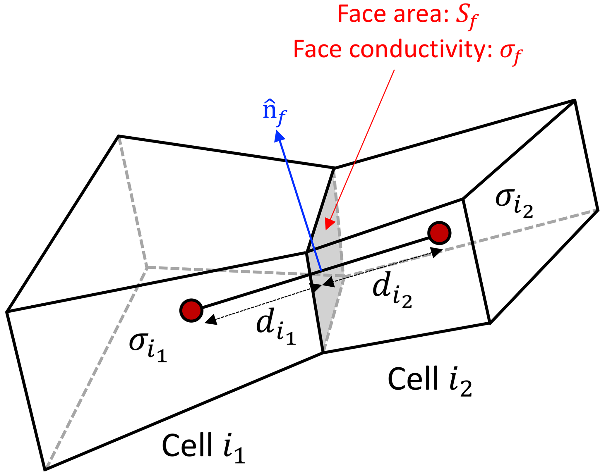
Figure 1Two adjacent FV cells i1 and i2 having conductivity and , respectively. The distances of the common face f from the center of cells i1 and i1, respectively, are and .
Let us consider the governing Poisson equation (Eq. 1) and integrate it over the ith cell of the domain Γ. This gives
where Vi is the volume of the ith cell.
By applying the Gauss divergence theorem in Eq. (3) and using the translation property of the Dirac delta function, we get
where Si is the surface area of the bounding faces of the ith cell, and dS is a differential area on the bounding surface with a unit surface normal pointing outward.
If the ith cell is bounded by Nf faces, Eq. (4) can be replaced by an equivalent discrete form
where f represents faces and Sf is the area of the bounding face f.
Using a two-point flux approximation for each face term in Eq. (5) by considering two adjacent cells i1 and i2 shown in Fig. 1, we get
where Snf is the area of the common face f projected onto the plane normal to the vector connecting centers of cells i1 and i2.
The conductivity at the face, σf, can be obtained by averaging the conductivity of cells i1 and i2. We use the following harmonic distance-weighted scheme to calculate σf:
where and are the conductivities of cells i1 and i2 and and are the distances of the projected face from the center of cells i1 and i1, respectively (Fig. 1).
The value of the flux at the face f, i.e., (∇ϕ)f, is obtained by using the approximation
Substituting Eqs. (7) and (8) in Eq. (6) and assuming that the computational domain Γ is subdivided into Nm FV cells, i.e., , where Γi⊂ℝ3 is the ith cell domain, we have
where Ai,k is the local coefficient matrix and si is the source vector for the ith cell.
The assembly of the local coefficient matrix into a global system, upon carrying out the summation in Eq. (9), results into the system of linear equations
where is the symmetric system matrix resulting from the FV discretization of Eq. (1), is a vector containing the unknown electric potential for all cells, and is the source vector resulting from the right-hand side of Eq. (1). To solve this linear system, we utilize various options of iterative solvers available from PETSc. Each electrode in an ERT survey results in a different vector s. Thus, for Ne electrodes, we need to solve Eq. (10) for Ne times with a different right-hand side. The solutions provide electrical potential at each cell center of the discrete computational domain and for each current injection location. Finally, the potential distribution for any combination of source/sink electrodes can be obtained by subtracting the potential associated with the sink electrodes from the source electrode potential (Johnson et al., 2010).
ERT inversion is a procedure of estimating electrical conductivity of the earth from a set of observed ERT data and/or some imposed constraints. The ERT inverse problem is a nonlinear optimization problem. For large-scale 3D ERT data, the inversion is often performed iteratively by linearizing the problem at each iteration. This section details our approach of performing inversion of ERT data.
3.1 Optimization problem
We pose the inverse problem as a nonlinear minimization problem of finding a conductivity model
where is an unknown model parameter vector in the model set M. Since the conductivity within subsurface can vary over several order of magnitudes, the inversion operations are performed for logarithmic conductivity, i.e., we assume m=ln σ. This also enforces positivity of conductivity values. The quantity ψ is the cost function, defined as
where ψd is the data cost function that represents a measure of the misfit between the observed dobs and synthetic dsyn ERT data, ψm is the regularization cost function representing a measure of the variation in the model parameters, and β is a regularization parameter.
A least-squares method is used to minimize ψ (Nocedal and Wright, 2006). Thus, ψd and ψm can be expressed as
where vectors dobs and dsyn are Nd dimensional vectors containing the observed and synthetic ERT data. is the data weighting matrix, usually a diagonal matrix, whose elements are estimated based on the standard deviation of the noise; is the regularization matrix, and mref is a Nm dimensional vector containing the logarithmic of reference conductivity model parameters.
3.2 Gauss–Newton method
To find a minimizer minv of the cost function in Eq. (12), we use a Gauss–Newton minimization approach. This is an iterative approach where after linearizing ψ(mk) in the vicinity of a model mk for a small model perturbation δmk at the kth iteration, we obtain a set of linear equations or the normal equation
where the Gauss–Newton Hessian matrix is given by
and the gradient vector by
The matrix 𝓙k is the Jacobian matrix also known as the sensitivity or the Fréchet derivative matrix. Following Johnson et al. (2010), we implement a parallel conjugate-gradient least-square (CGLS) solver (Hestenes and Stiefel, 1952) to solve the normal Eq. (15). The normal equation is first reformulated into an equivalent least-squares problem and then solved for the model update δmk using only the Jacobian matrix 𝓙k without explicitly forming the Hessian matrix 𝓗k. As Nm≫Nd for typical ERT surveys, this approach avoids the massive computational cost associated with the explicit formation of 𝓗k. We therefore only need to compute 𝓙k at each iteration, which is also a computationally intensive step. The effective computation of 𝓙k is explained in the next subsection (Sect. 3.3).
The solution of Eq. (15) gives a model update vector δmk at the kth iteration such that a new model
decreases the cost function ψ, i.e., . There is a common practice to find step length α using a line search method (Nocedal and Wright, 2006); however, from our experience, a full step length, i.e., α=1, works well for the ERT data inversion.
In our implementation, the Gauss–Newton iteration usually starts with an average apparent conductivity model as an initial model and continues until the data misfit drops below a predefined tolerance level (defined by a chi-squared data misfit ) or it reaches a predefined maximum number of iterations. Furthermore, a predefined input conductivity model can also be used as an initial model if it can be estimated from the existing geological and/or geophysical information. After the inversion converges, it provides the minimizer minv which represents the inverted conductivity model σinv=exp (minv).
3.3 Jacobian computation
Calculating 𝓙 at each iteration is one of the most computationally intensive steps in Gauss–Newton inversion. Therefore, an efficient 𝓙 drives the robustness of the developed inversion scheme and maximizes its scalability. The Jacobian matrix characterizes the change in the synthetic ERT data dsyn relative to a change in the model parameters m and is defined as the partial derivatives of dsyn with respect to m=ln σ; i.e.,
An adjoint state method is used to effectively compute the Jacobian matrix. Let A and B be the source and sink electrodes located at rA and rB and M and N be the two measuring or receiving electrodes located at rM and rN. The potential difference between M and N can be obtained using the potential computed due to the source A at M and N, i.e., ϕAM and ϕAN, and the sink B at M and N, i.e., ϕBM and ϕBN. A simplified four-electrodes Wenner configuration is shown in Fig. 2. Note that, contrary to this configuration, electrodes can be placed in any other configurations, e.g., Schlumberger, pole–pole, pole–dipole, dipole–dipole, and gradient arrays (Dahlin and Zhou, 2004).
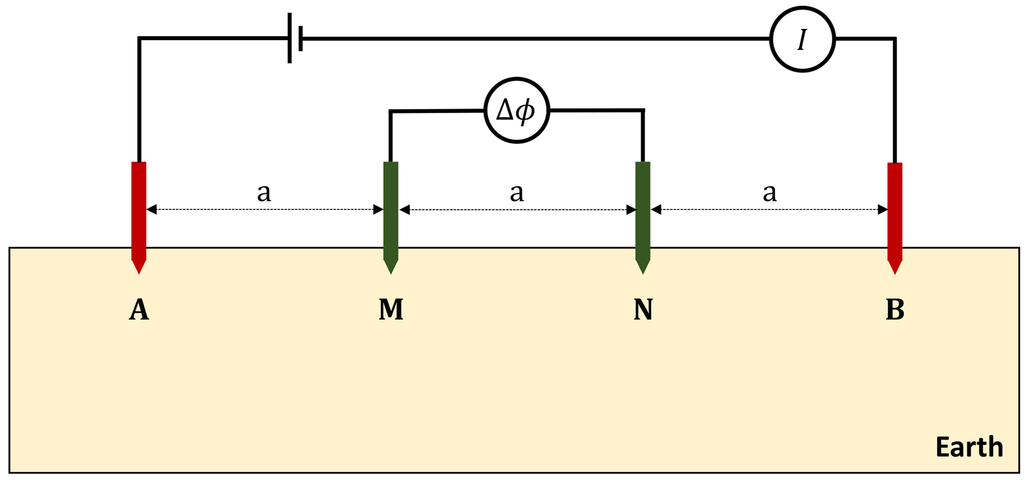
Figure 2Wenner electrode configuration: four electrodes A, B, M, and N are deployed in-line with an equal spacing a between the two neighboring electrodes. Electrodes A and B act as the source and sink electrodes where current I is injected, while electrodes M and N act as the receiving electrodes measuring a potential difference Δϕ.
Using the expression derived in Appendix A (Eq. A9), an element of the Jacobian matrix is obtained by
where ϕA and ϕB are potential distributions due to the source A and sink B and ϕM and ϕN are potential distributions due to pseudo-source and pseudo-sink, respectively, at the receiving electrodes M and N.
Assuming and , where ϕS is the net potential due to the source and sink electrodes A and B, and ϕR is the net potential due to source and sink assumed to be located, respectively, at the receiving electrodes M and N, this results in
Equation (21) is valid for any numbers of the source/sink electrodes and the receiving electrodes as well as any of their combinations. One only needs to compute the net potentials due to the source/sink electrodes ϕS and receiving electrodes ϕR using the superposition principle.
The parallel implementation strategy for the ERT forward modeling and inversion capabilities follows the existing PFLOTRAN’s strategy for flow and transport process models. Forward ERT modeling is implemented by extending PFLOTRAN's hierarchy of Fortran classes and data structures to create a new ERT process model that constructs and solves the linear systems of equations described in Sect. 2. The implementation of inversion, as described in Sect. 3, is completely new to PFLOTRAN and requires all the necessary steps (or calculations) for ERT inversion, such as the cost-function computation, regularization, Jacobian computation, solution to the dense Gauss–Newton normal equation, and model update.
To execute simulations in parallel, domain decomposition is employed to distribute the discrete computational domain across (computer) processes using a division along the three principal axes for structured grids (calculated by PETSc or explicitly defined by the user), or in the case of unstructured grids, the ParMETIS parallel graph partitioner (Karypis and Schloegel, 2013) is employed to divide the domain. All interprocess communication is carried out with MPI (Message Passing Interface), and PETSc's parallel data structures facilitate much of the MPI communication.
Efficient partitioning and the overlapping of communication with computation (e.g., calculating floating point operations while data are being transferred between processes) helps improve parallel performance. The latter helps mask communication costs. The goal is to maximize the time spent in computation and minimize interprocess communication and enforce load balance, the even distribution of computation across processes employed. Efficient partitioning can be accomplished by dividing the domain evenly and minimizing the number and size of (MPI) messages being passed between processes. However, an even distribution does not necessarily guarantee load balance as certain regions of the domain with time-consuming operations (e.g., localized physics, intense input/output or I/O) may require more computation. Thus, efficient partitioning is not trivial.
PFLOTRAN's parallel file I/O is through HDF5 (Hierarchical Data Format version 5), a platform-independent binary file format that leverages MPI-IO operations to read/write a single file using multiple (potentially thousands of) processes (The HDF Group, 2022). PFLOTRAN writes ASCII-formatted observation files (files storing ERT data at specific locations in space) locally on the processes owning the observation points. Thus, the writing of observation files requires no parallel communication. For more comprehensive details on the parallel implementation strategy employed within PFLOTRAN, interested readers are referred to Hammond et al. (2012, 2014).
To examine the accuracy of the PFLOTRAN ERT process model, simulation results are compared to solutions obtained using well-established analytical and numerical methods. Two cases are considered for the comparison: three-layer earth and 3-D earth resistivity models. All benchmarking simulations were performed on the Deception supercomputer housed at the Pacific Northwest National Laboratory. It is composed of 96 compute nodes where each node has 64-core AMD EPYC 7502 processors running at 2.5 GHz boost to 3.35 GHz with 256 GB of memory.
5.1 Layered earth model
Let us consider the layered earth or 1D model shown in Fig. 3. The model is composed of three layers, whose resistivity (ρ) and thickness (t), i.e., [ρ, t] are [100 Ωm, 30 m], [300 Ωm, 30 m], and [10 Ωm, half space] from the top to bottom. The dimension of the model is m3. The model boundaries are extended to ±3000 m in the x and y directions and 3000 m in the z direction to accommodate zero Dirichlet boundary conditions at the side and bottom boundaries. These boundary extensions are not shown in Fig. 3. Vertical electrical sounding (VES) data are simulated at the center of the model considering a Wenner configuration. This configuration consists of four electrodes A, B, M, and N, which are deployed in-line with an equal spacing a between the two neighboring electrodes (Fig. 2). Electrodes A and B again act as the current source and sink electrodes, while electrodes M and N act as the potential receiving electrodes. Starting with a smaller value of a for a shallow-depth investigation, the value is progressively increased to examine deeper depths. In our case, we start with a minimum value amin=8 m and progressively increase it to a maximum amax=132 m following , where δa=4 m and . This results in Nd=32 VES sounding recordings using Ne=128 electrodes.
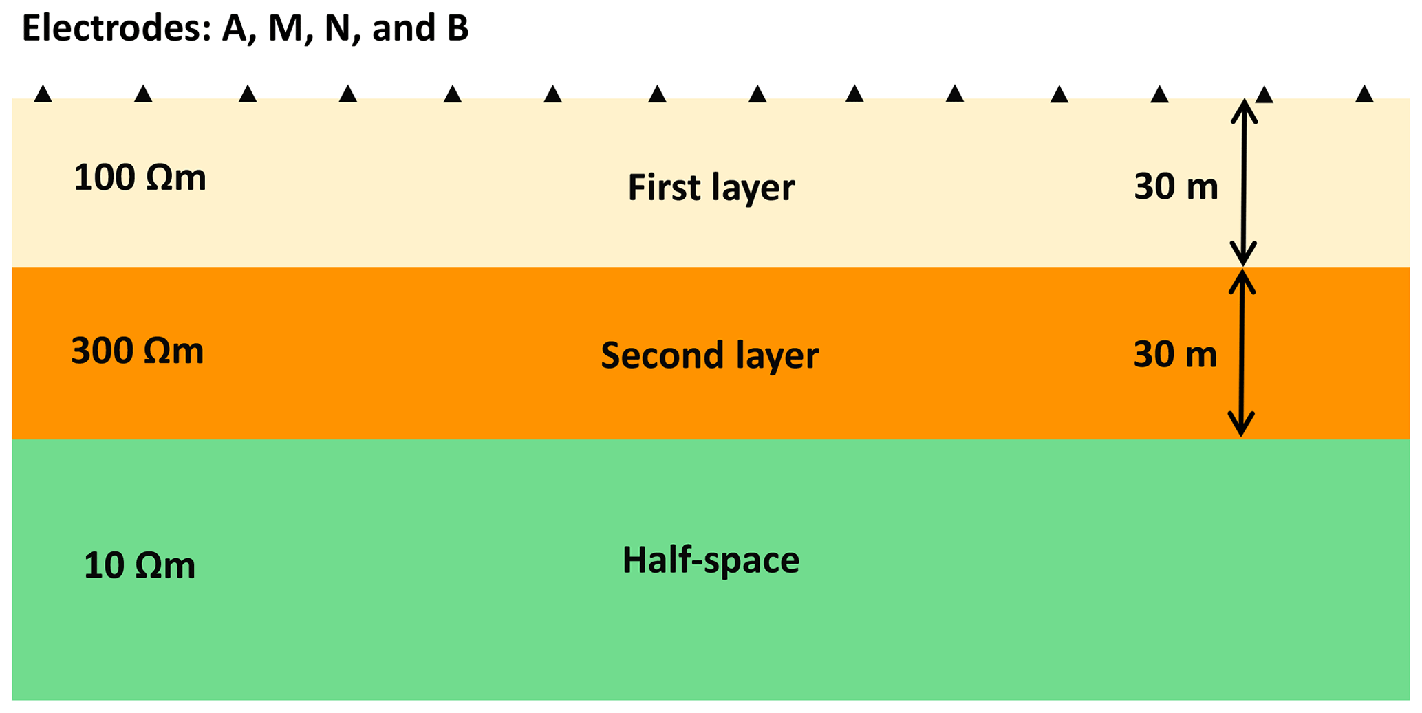
Figure 3Vertical cross section of a three-layer earth resistivity model used for benchmarking PFLOTRAN results against the analytical solutions.
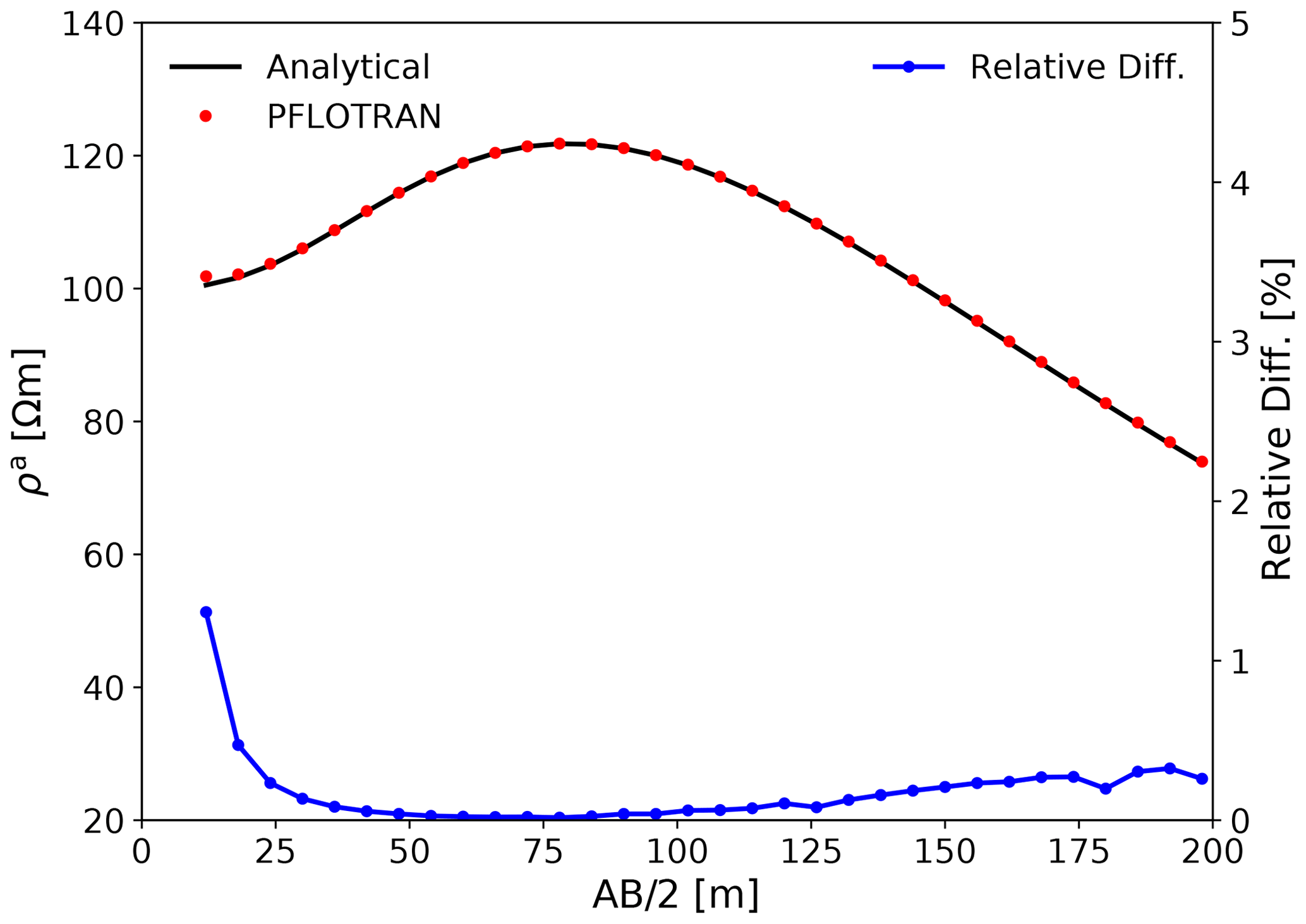
Figure 4Apparent resistivity ρa responses computed for the layered earth resistivity model in Fig. 3 (upper plot). They are calculated using the analytical method (solid black lines) and PFLOTRAN (filled red circles). The lower plot (blue line) shows the relative difference (in percentage) between the analytical and PFLOTRAN results.
To simulate the VES data, the model is discretized using a mix of uniform and non-uniform cell sizes in the x, y, and z directions. The main computational domain is discretized with a uniform grid spacings of 2 m in the x and y directions and 1 m in the z direction. The boundary regions are discretized with severely stretched non-uniform grid spacings following Jaysaval et al. (2014). The discretization results in a grid with cells. Therefore, using the FV method to simulate electric potentials leads to a system of linear equations with 6 912 000 DOFs. PFLOTRAN simulated the VES data using 512 processes on Deception. The total simulation time was 45 s.
The simulated VES results are compared to analytical solutions obtained from SimPEG (Cockett et al., 2015). Figure 4 shows the comparison of the apparent resistivity ρa responses. Analytical and PFLOTRAN results are shown by the solid black line and filled red circles, respectively. We observe that both responses agree very well. To make the comparison more quantitative, we calculate the relative difference between the two responses and show the difference in Fig. 4 (blue line). The relative difference varies from 0.02 % to 1.3 %. We also calculate the average relative difference using
where ρa with subscripts 1 and 2, respectively, represents the apparent resistivity computed using PFLOTRAN and the analytical method from SimPEG. The average relative difference ϵ is 0.18 %. These relatively small differences demonstrate the high degree of accuracy of the PFLOTRAN ERT process model for the 1D model. Note that the apparent resistivity was computed using
where and G is a geometric factor given as
where distances between the source electrode A and the receiving electrodes M and N are, respectively, rAM and rAN, while those between the sink electrode B and the receiving electrodes M and N are, respectively, rBM and rBN. For the Wenner configuration, rAM=a, rAN=2a, rBM=2a, and rBN=a. Therefore, geometric factor was used for calculating ρa using Eq. (23).
5.2 Three-dimensional earth model
In the previous example, PFLOTRAN accuracy for simulating ERT responses was validated for a simplistic 1D earth model. In the real world, however, the earth models are 3-D with varying degrees of heterogeneity. Therefore, it is important to validate the accuracy of numerical results computed using PFLOTRAN against results computed using well-established methods for 3D models.
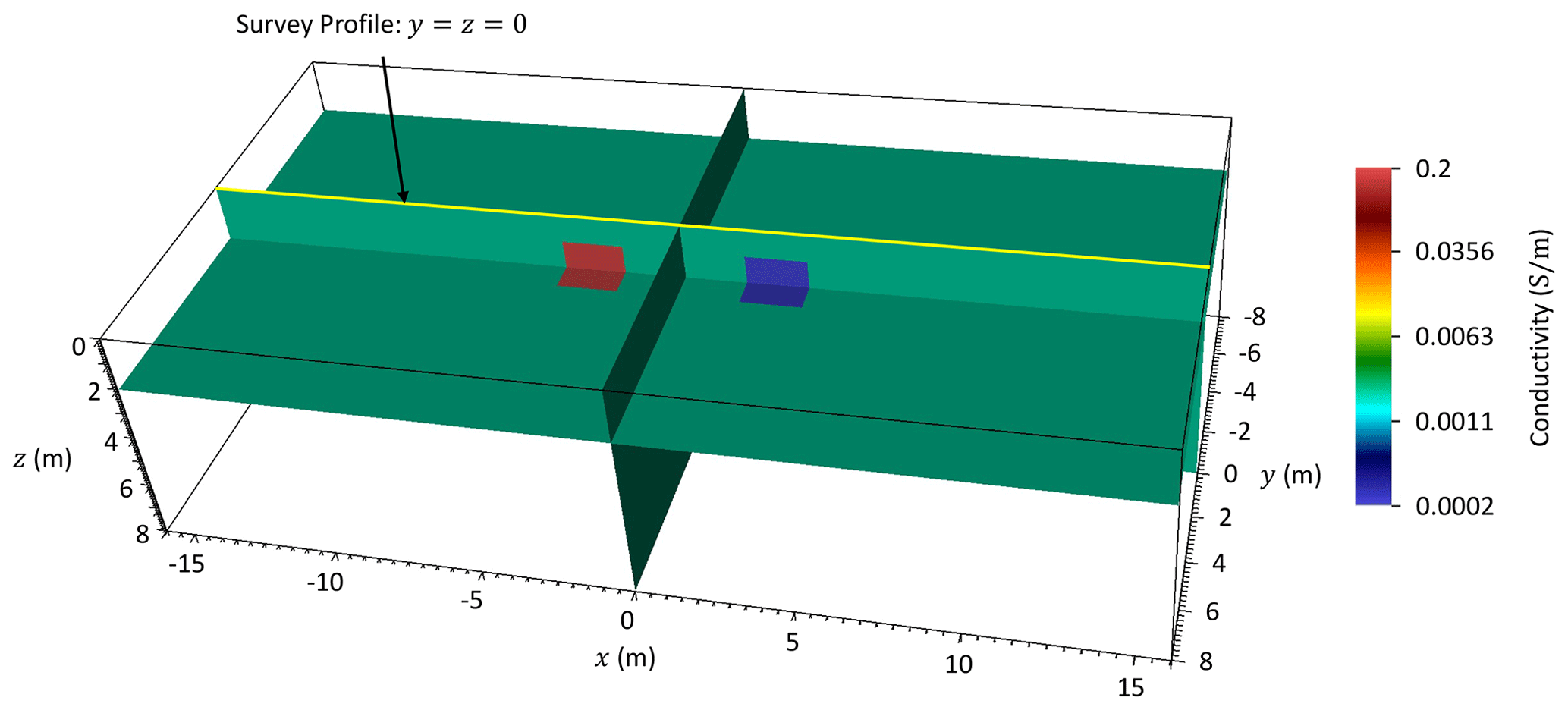
Figure 5Three-dimensional earth resistivity model composed of two anomalous blocks embedded in a homogeneous background. ERT profiling data are simulated along a survey profile at m from m to x=16 m using the Wenner configuration with increasing electrode spacing a from 1 to 6 m.
We consider the 3D model shown in Fig. 5. The model dimension is m3. It has a homogeneous background of conductivity 0.002 Sm−1 and includes two anomalous blocks: a conductive block (0.2 Sm−1) and a resistive block (0.0002 Sm−1). Both anomalous blocks have a dimension of m3 and are separated by 4 m in the x direction. As in the previous case, the model boundaries are extended to ±1000 m in the x and y directions and 1000 m in the z direction to accommodate zero Dirichlet boundary conditions at the side and bottom boundaries. ERT profiling data are simulated along a survey profile (yellow line) at m from m to x=16 m using the Wenner configuration with increasing electrode spacing a from 1 to 6 m. Unlike the VES performed for the 1D model where data were simulated at a single observation point at the center of the model, the ERT profiling, performed for the 3D model, records data at multiple observation points along the survey profile. The profiling, therefore, helps in investigating lateral conductivity variations in the model along the x direction. In this case, it results in Nd=129 ERT data recording by using Ne=32 electrodes placed uniformly at every 1 m from m to x=15.5 m.
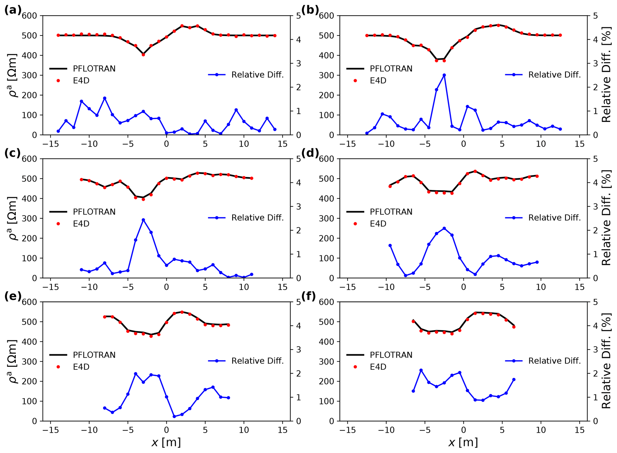
Figure 6Apparent resistivity ρa responses computed for the 3D earth resistivity model in Fig. 5 using the Wenner configuration with spacings: (a) a=1 m, (b) a=2 m, (c) a=3 m, (d) a=4 m, (e) a=5 m, and (f) a=6 m (upper plots). They are calculated using PFLOTRAN (solid black lines) and E4D (filled red circles) for an ERT profiling along a survey profile at from m to x=16 m. The lower plots (blue lines) show the relative difference (in percentage) between PFLOTRAN and E4D results.
The main computational domain is discretized with a uniform grid spacing of 0.2 m in all the three directions, while the boundary domain is again discretized with severely stretched non-uniform grid spacings. The model discretization leads to a grid with FV cells and, hence, 1 440 000 DOFs in the corresponding system of linear equations. PFLOTRAN simulated the ERT profiling data using 128 processes on Deception. The total simulation time was 9 s.
Figure 6a–f (upper curves) show the apparent resistivity ρa responses computed for the 3D model in Fig. 5 using the ERT profiling with the Wenner configuration with electrode spacings of 1, 2, 3, 4, 5, and, 6 m. The solid black lines show the responses computed using PFLOTRAN. All responses exhibit the characteristics of the conductive and resistive anomalous blocks embedded in a homogeneous background of conductivity 0.002 Sm−1 or resistivity 500 Ωm; see, e.g., the low apparent resistivity on the left and high apparent resistivity on the right sides of the plots. These responses are compared to responses computed using E4D (Johnson et al., 2010; Johnson and Wellman, 2015). In E4D, an unstructured-mesh FE method is implemented to perform the forward modeling. The filled red circles show the responses computed using E4D. The relative differences between the two codes are shown by the lower blue lines, which vary from 0.02 % to 2.5 %. The average relative difference ϵ computed using Eq. (22) is 0.77 %. These relatively small differences imply a good agreement between responses computed using both codes.
To examine the efficiency of PFLOTRAN to invert ERT data, we consider a model modified from Fig. 5 by cropping the model for m. The modified model, therefore, has the dimension of m3. The model is discretized using the same grid spacings as in the previous 3D modeling example, which resulted in FV cells. We computed synthetic ERT data for three survey lines located at the ground surface at m, y=0 m, and y=5 m from m to x=8 m. Electrodes are placed uniformly with an electrode spacing of 1 m along the three survey lines from m to x=7.5 m, i.e., 16 electrodes along each survey line. Using these Ne=48 electrodes, ERT data were simulated considering different combinations of a set of 4 electrodes, where 2 electrodes acted as the current and the remaining 2 as the potential receiving electrodes. These electrode combinations result in Nd=2070 simulated ERT data. PFLOTRAN simulated these ERT data using 128 processes on Deception. The total simulation time was 6 s. In this case, ERT data were simulated in the form of the resistance obtained using , which basically equals to the potential difference Δϕ for unit current (I=1 A).
The simulated ERT data were then inverted using PFLOTRAN starting with a model having a half-space conductivity of 0.0022 Sm−1. The starting model conductivity was obtained by averaging the apparent conductivity computed from the given ERT data. The previously described modeling grid also acted as the inversion grid; i.e., each cell in the model was used as an inversion parameter. Therefore, we needed to invert for Nm=864 000 model parameters. PFLOTRAN inverted the ERT data using 512 processes on Deception. The total inversion time was 74 s.
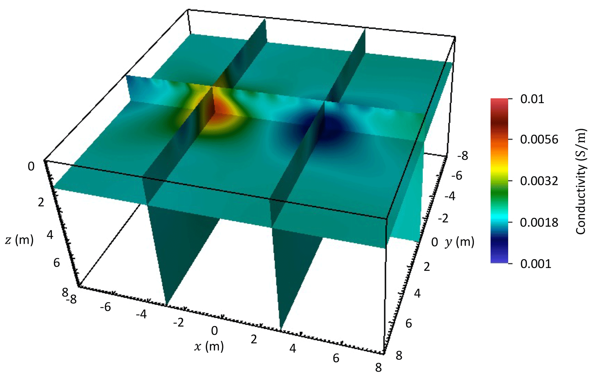
Figure 7Inversion result of the simulated ERT data for a model modified from Fig. 5 by cropping the model for m.
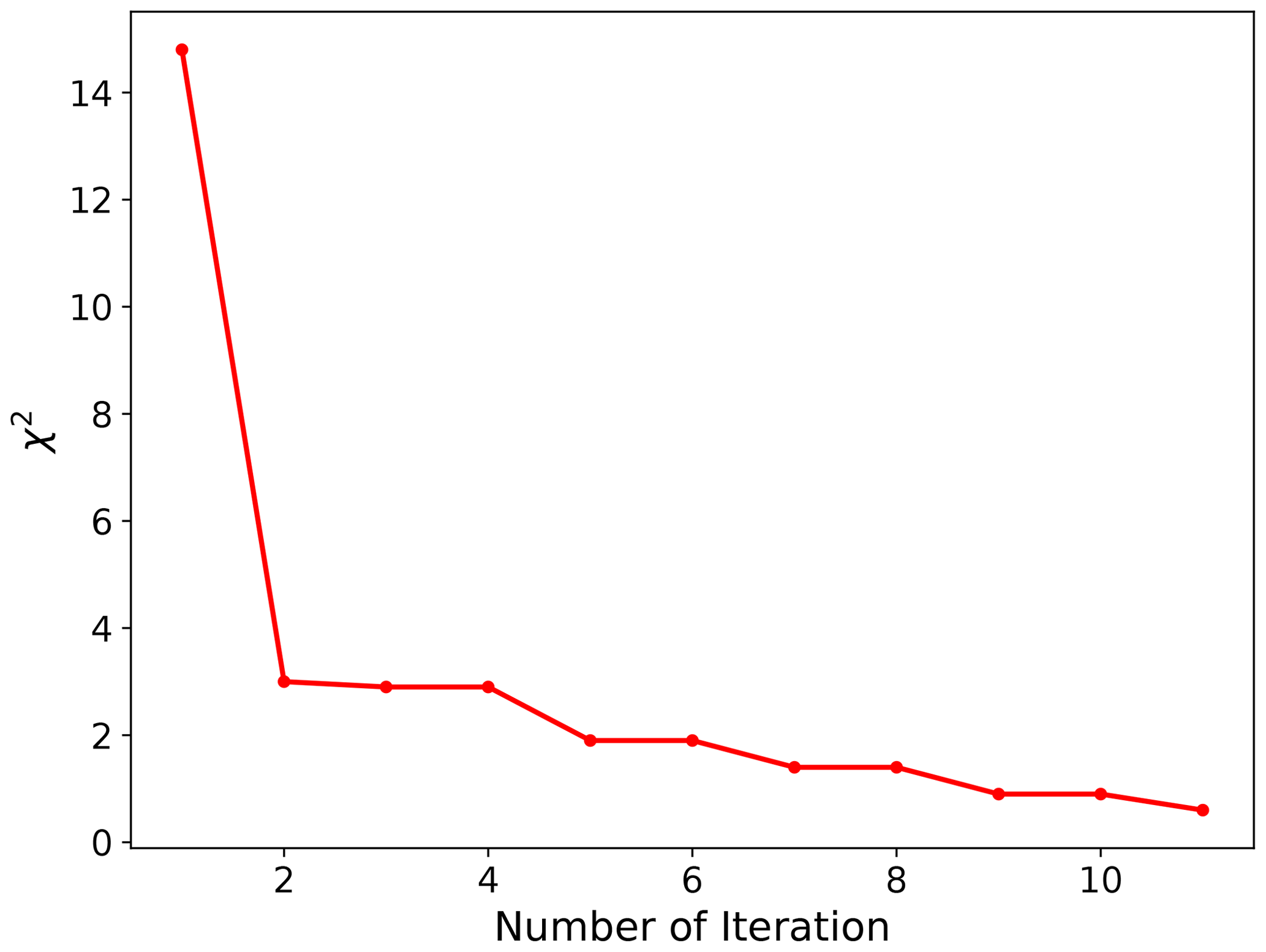
Figure 8A measure of data misfit as the inversion progresses: χ2 versus number of iteration.
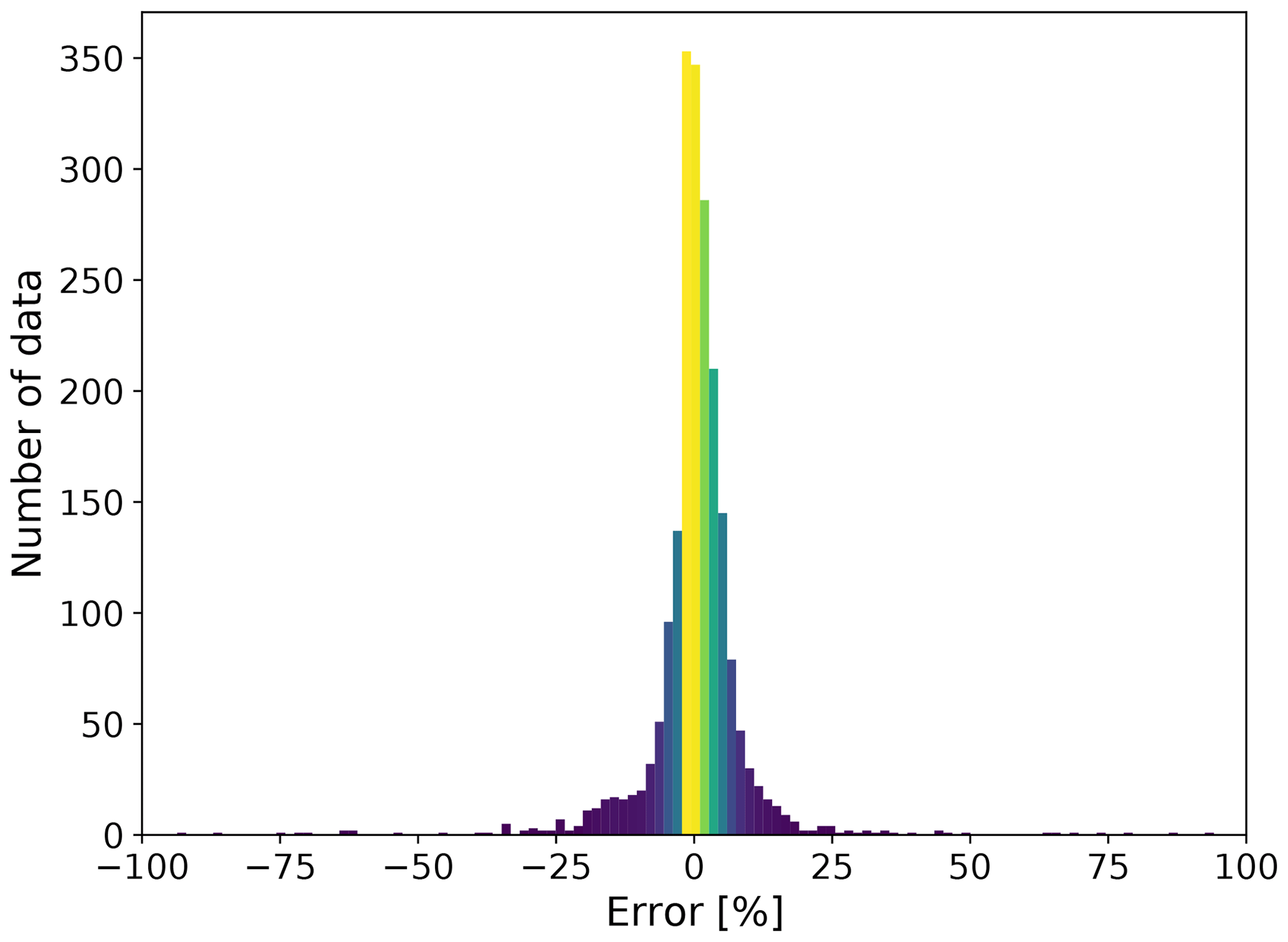
Figure 9Histogram of data-fit error, which is defined as ratio of the residual resistance (difference in the observed and predicted resistances) and observed resistance expressed as a percentage.
Figure 7 shows the inverted conductivity model. The inverted model agrees well with the true model: the inversion recovered the conductive and resistive anomalies in the model. The inverted resistivity, however, varies smoothly in the model because a smooth regularization constraint is applied by minimizing the difference in the cell conductivity and the conductivity of its neighboring cells. Further discussion on the implementation of our regularization schemes is beyond the scope of the current paper.
The initial chi-squared data misfit χ2 was 14.8. As the inversion progressed, χ2 decreased as shown in Fig. 8. The inversion took 11 iterations to satisfy the convergence criteria defined by χ2≤0.9. To further examine the efficiency of PFLOTRAN to fit the individual ERT data, a histogram of data-fit error is also shown in Fig. 9. The data-fit error is defined as ratio of the residual resistance (difference in the observed and predicted resistances) and observed resistance expressed as a percentage. The histogram implies that the ERT data were fitted comparatively well.
Scalability tests demonstrate parallel performance or how efficiently a simulator utilizes additional processes to either speed up a simulation of fixed problem size (strong scaling) or maintain speed as the problem size and number of processes increase proportionally (weak scaling). For ideal strong scaling, the speedup is proportional to the increase in the number of processes (e.g., doubling the number of processes cuts the run time in half), while ideal weak scaling results in an unaltered or constant run time. In either (ideal) case, the additional computing capacity is efficiently utilized. Ideal strong scaling is often termed linear speedup, whereas superlinear speedup is better than ideal (e.g., doubling the number of processes reduces the run time to less than half). Superlinear performance is not uncommon, as access to an increased cache (efficient, high-performance memory on the processor core) can generate superlinear speedup.
As discussed earlier, there are two computationally intensive steps to invert ERT data: forward modeling and Jacobian computation. To demonstrate the parallel performance of PFLOTRAN for these two steps, large-scale strong scaling tests are reported in this section by using up to 1024 processes on the Deception supercomputer or up to 131 072 processes on the Theta supercomputer. Configuration details for Deception were previously given in the “Modeling benchmarking results” section (Sect. 5). On the other hand, Theta is a leadership-class supercomputer, ranked within the top 100 fastest computers in the world and housed at the Argonne Leadership Computing Facility (ALCF) at Argonne National Laboratory (https://www.alcf.anl.gov/alcf-resources/theta, last access: 27 January 2023). With a peak performance of 11.7 PFLOPS, it is composed of 4392 compute nodes connected through a Cray Aries network. Each node has 64-core Intel Xeon Phi 7230 processors running at 1.3 GHz with 192 GB of memory. Therefore, there are 281 088 processes available on Theta. The PFLOTRAN compilations on Deception and Theta were linked to Intel's Math Kernel Library (MKL). The code leverages solely the distributed-memory parallel capability on the machines and not the shared-memory multi-threading.
7.1 Forward modeling scalability
The three-layer earth model in Fig. 3 is first rediscretized to generate several test matrices for the analysis by considering different cell sizes in the x, y, and z directions. These test matrices result in six different modeling scenarios from coarser to finer grids. Table 1 completely specifies details of the test matrices M2, M7, M19, M35, M64, and M122 along with the number of DOFs in the governing matrix equations that ranges between 2 ×10⁶ and 122 ×106. The naming of these matrices is based on the number of DOFs they represent; e.g., M19 represents a matrix equation with about 19 ×106 DOFs. To the best of our knowledge, the modeling with 122 ×106 DOFs stands as the largest ERT modeling reported in the geophysical literature. The next largest 3D ERT modeling problem reported in the literature was composed of about 10 ×106 DOFs (Ren et al., 2018), while most others were often composed of less than 1 ×10⁶ DOFs (Günther et al., 2006; Rücker et al., 2006; Johnson et al., 2010; Johnson and Wellman, 2015). Having the capability to solve for up to a 100 ×106 DOFs efficiently in parallel is a crucial requirement for large-scale ERT modeling and inversion problems in the future if model dimensions are significantly increased and/or finer grids are employed.
Table 1Test matrices obtained by rediscretizing the three-layer earth model in Fig. 3 using different cell sizes dx, dy, and dz in the x, y, and z directions. Nx, Ny, and Nz are, respectively, the number of FV cells in the x, y, and z directions. Note that the cell sizes are given only for the main computational domain; the boundary domain is discretized using severely stretched non-uniform cell sizes.
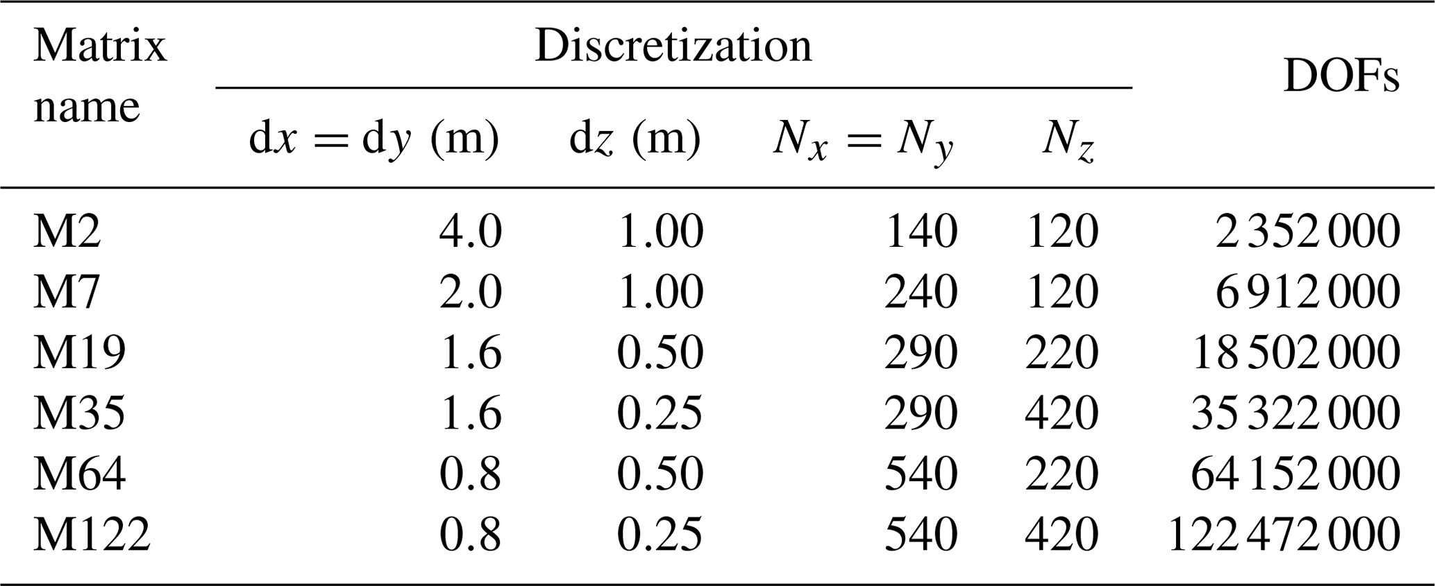
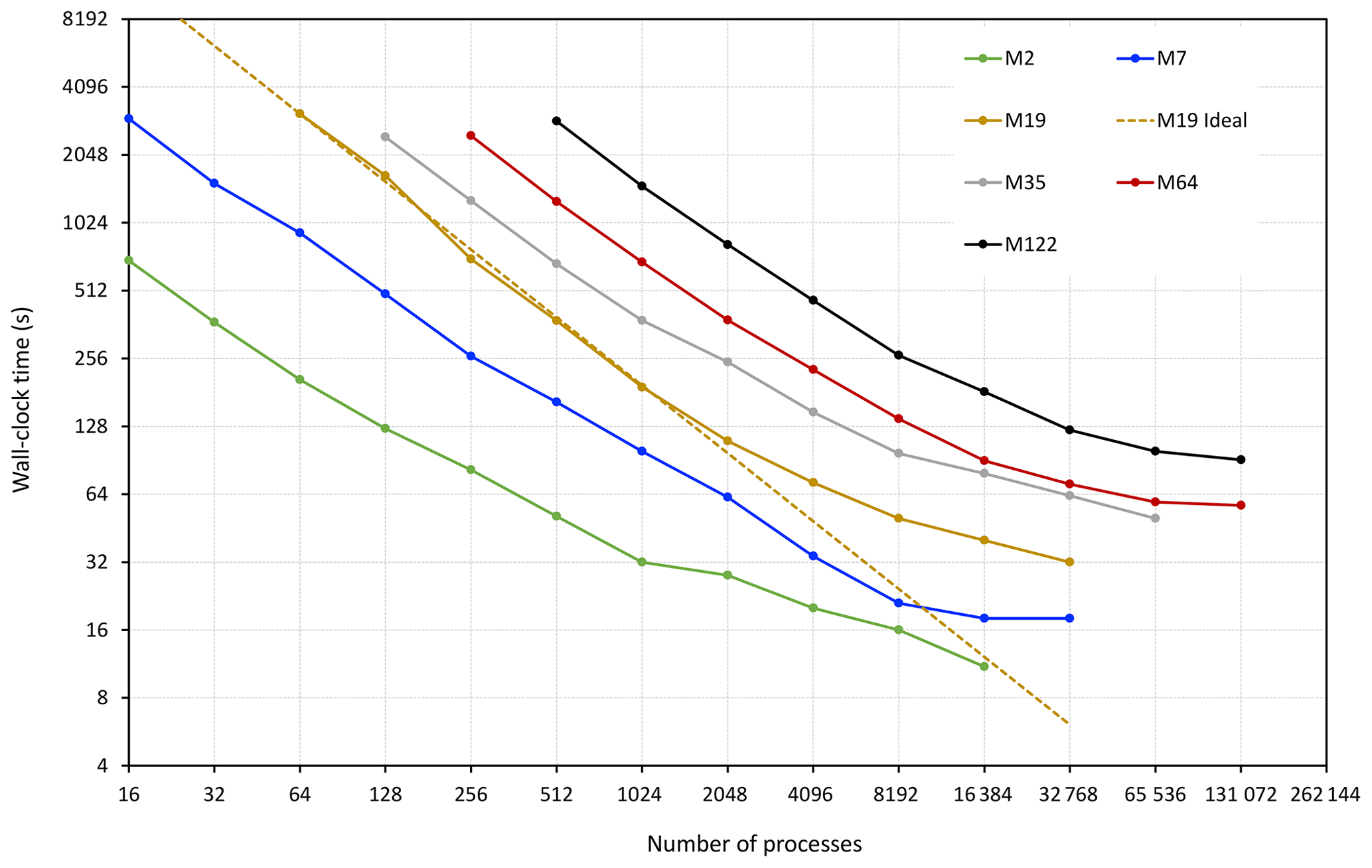
Figure 10PFLOTRAN scalability for simulating ERT data for the model in Fig. 3 for Ne=128 electrodes. The test is performed on the Theta supercomputer considering six test matrices M2, M7, M19, M35, M64, and M122 with the respective number of DOFs of about 2, 7, 19, 35, 64, and 122 ×106 (see Table 1 for details).
Considering the six test matrices above, we performed the forward modeling scalability test on Theta for simulating ERT data for Ne=128 electrodes, the same number of electrodes as in the three-layer benchmarking example. Figure 10 illustrates the PFLOTRAN ERT process model strong scaling for each test case (wall-clock time versus the number of processes employed for a fixed problem size). The wall-clock time is shown on the vertical axis, while the horizontal axis shows the number of processes; both axes are shown in logarithmic base-2 scale. The line labeled “M19 Ideal” is the plot of ideal performance based on the 64 process run time for the M19 simulation:
where Tn is the time on n processes and T64 is the time on 64 processes.
For all problem sizes, the wall-clock times flatten at higher numbers of processes. This phenomenon is expected as the amount of work per process (DOFs per process) decreases at higher process counts and the cost of communication between processes begins to dominate. The M19 performance begins to deviate from ideal at ∼2048 processes, which equates to ∼9000 DOFs per process. Similar behavior is observed for many of the other problem sizes. Hammond et al. (2014) demonstrate that for groundwater flow and reactive transport simulation PFLOTRAN runs most efficiently when at least 10 000 DOFs are assigned to each process. These results show that this 10 000 DOF threshold also applies for PFLOTRAN ERT simulations. That is, PFLOTRAN's scalability on the supercomputer should be more ideal when the number of DOFs per process is greater than 10 000.
Another factor limiting parallel performance is the limited scalability of linear Krylov solvers at high process counts. Mills et al. (2009) demonstrates that the vector inner products performed within Krylov solvers become increasingly expensive as tens of thousands of processes are employed to solve a problem. These inner products (or MPI global reduction operations) require repeated global synchronization across all processes involved. As more processes are employed to solve the problems (requiring communication across a growing network of compute nodes), the transfer of information for each vector inner product is more expensive time-wise (i.e., increased number of hops within the high-speed network, longer distance traveled). Figure 10 reveals a similar phenomenon.
7.2 Jacobian computation scalability
To test the scalability of PFLOTRAN for the Jacobian computation, we consider a Jacobian matrix computed for inverting the ERT data in the “Inversion result” section (Sect. 6). Recalling that Nd=2070 ERT data and Nm=864 000 model parameters for the inversion example, the dimension of the Jacobian matrix 𝓙 is therefore 2070×864 000. The Jacobian matrix is computed at each inversion iteration after the forward modeling run and used in the normal equation (Eq. 15) to get a model update δm.

Figure 11PFLOTRAN strong scaling for computing the Jacobian for the ERT inversion example in Fig. 7. The dimension of the Jacobian matrix 𝓙 is 2070×864 000 and is distributed uniformly over each computing process. PFLOTRAN exhibits superlinear performance for larger numbers of processes.
The Jacobian scalability test is performed on the Deception supercomputer. Figure 11 illustrates the strong scalability of PFLOTRAN wall-clock time for computing 𝓙. It shows that PFLOTRAN exhibits linear (and sometimes superlinear) scalability for computing 𝓙 with increasing numbers of processes. Consequently, the total wall-clock time for computing 𝓙 using 1024 processes reduces to 0.5 s compared to 887 s when using a single process on Deception. This ideal performance in computing 𝓙 is most likely due to even load balance across processes and the lack of MPI communication in its construction. Moreover, as noted before, the superlinear performance is most likely due to access to increased cache with an increasing number of processes.
For large-scale ERT inversion problems, the linear scaling for computing 𝓙 can be exploited to reduce the overall inversion wall-clock time even if PFLOTRAN exhibits deteriorating scalability for the forward modeling on a very large number of processes. For example, for an ERT inversion problem where the 𝓙 calculation time is much higher than the forward modeling time, increasing the number of processes to reduce the overall inversion wall-clock time is recommended, even when forward modeling exhibits a significant departure from the linear scalability. One has to find a balance between the two, and the most time-consuming operation should govern.
In the past 20 years, a few open-source 3D ERT modeling and inversion codes were developed to handle moderate-scale ERT problems (e.g., ResIPy, SimPEG, pyGIMLI, and E4D). Although some of these codes can practically tackle most present ERT modeling and inversion problems having less than 10 ×106 DOFs, they still lack full-scale parallel implementations to efficiently distribute numerical computations over massive supercomputers. The limitation can also lead to computational challenges for large-scale ERT problems with 100 ×106 or more DOFs, which may not be solved efficiently with the existing codes. The 3D ERT modeling and inversion capability developed within PFLOTRAN removes this limitation. To examine the accuracy of the forward modeling capability, numerical results from PFLOTRAN were compared to analytical solutions for a layered earth model and numerical results obtained from E4D for a 3D earth model. The average relative differences stayed within 1 %, which demonstrated the high degree of accuracy of the PFLOTRAN modeling capability. Furthermore, large-scale strong scalability tests, using up to 131 072 processes, were performed on a leadership class supercomputer to demonstrate efficient distribution of computational workloads over massive supercomputers. The scalability tests demonstrate that computational times for the Jacobian computation scale linearly with increasing number of processes. For the forward modeling, PFLOTRAN showed a linear to near-linear scaling behavior up to 10 000 DOFs per process, beyond which performance tends to degrade.
Due to the efficient parallel performance of PFLOTRAN observed above, a large-scale ERT simulation problem with 122 ×106 DOFs and 122 electrodes could be solved in about 2 min by using 32 768 processes as compared to taking about 1 h with 512 processes. Combining this forward modeling scalability along with the ideal scaling of the Jacobian computation, we can aim for inverting moderate-scale ERT problems within minutes and large-scale problems within hours with the access to massive supercomputers. The moderate-scale inversion example of Sect. 6 demonstrated that inversion of Nd=2070 data and Nm=864 000 model parameters could be performed in about 1 min by using 512 processes.
Finally, there were two key motivations for implementing ERT capabilities in PFLOTRAN. The first motivation was to utilize the massive parallel infrastructure implemented within PFLOTRAN for the flow and transport simulations as illustrated by Hammond et al. (2012, 2014) for simulating subsurface problems composed of billions of DOFs utilizing hundreds of thousands of computing processors. This infrastructure made PFLOTRAN a natural fit to achieve our goal of massive parallel implementation for the ERT forward modeling and inversion capabilities. Researchers familiar with PFLOTRAN can now have immediate access to the added geophysical ERT capabilities with minimal learning efforts.
The second motivation was to have a native implementation of ERT modeling and inversion capabilities along with flow and transport simulations. The new capabilities will allow us to perform fully coupled hydro-geophysical simulations and inversion. The idea behind the joint hydro-geophysical simulation is to use known flow and transport parameters, such as porosity and intrinsic permeability, and simulate for hydrological variables, e.g., liquid saturation and solute concentration. Using petrophysical relationships (e.g., Archie's law or its modifications; Slater, 2007), these parameters and variables can be mapped into electrical conductivity, which subsequently can be used for simulating ERT responses. In our previous work, a joint hydro-geophysical simulation capability was developed by combining the capabilities of PFLOTRAN and E4D (Johnson et al., 2017). However, it was not straightforward to use PFLOTRAN–E4D for joint hydro-geophysical simulations. This is because the implementation was based on obtaining flow and transport parameters and variables from PFLOTRAN using a structured mesh, which then needed to be interpolated on an unstructured tetrahedral mesh for ERT simulations by E4D. The process was cumbersome and had the potential for errors. PFLOTRAN’s native implementation of ERT avoids employing any kind of interpolation because both flow and transport and ERT simulations use the same modeling grid.
Furthermore, there are growing interests in joint hydro-geophysical inversion, i.e., estimating the distribution of subsurface flow and transport parameters, from time-lapse ERT data; see, e.g., Mboh et al. (2012), Camporese et al. (2015), Rücker et al. (2017), González-Quirós and Comte (2021), and Pleasants et al. (2022). The inclusion of the ERT simulation capability in PFLOTRAN fulfills the requirement of the forward modeling necessary for native implementation of hydro-geophysical inversion. Fully coupled hydro-geophysical simulation and inversion capabilities are currently under development within PFLOTRAN and will be a focus of our forthcoming papers.
Two new capabilities – forward modeling and inversion of geophysical ERT data – are developed within PFLOTRAN, a massively parallel open-source, state-of-the-art, multi-phase, multi-component subsurface flow and transport simulation code. The capabilities are accurate, robust, and highly scalable on HPC platforms. The accuracy of the forward modeling capability was demonstrated for layered earth and 3D earth conductivity models by comparing our numerical results against well-established analytical and numerical results. The average relative differences stayed within 1 %, demonstrating the high degree of accuracy of the PFLOTRAN ERT process model. The inversion capability was demonstrated for a 3D synthetic case by recovering the conductivity of the model. Large-scale scalability tests illustrated that the forward modeling for models with 100 ×106 DOFs can be performed in a few minutes; e.g., ERT modeling for a model with 122 ×106 DOFs and 122 electrodes was performed in 128 s by using 32 768 processes on a supercomputer. The Jacobian computation, a key ingredient for the inversion, exhibited ideal or linear scaling, and as a result a Jacobian of 2070×864 000 dimension was computed in 0.5 s using 1024 processes compared to 887 s using a single process. Moreover, integration of geophysical ERT capabilities within PFLOTRAN opens the door to perform coupled hydro-geophysical modeling and inversion, which is a focus of our future research.
Let us assume that pM and pN are two interpolation vectors and ϕA and ϕB are potential distributions due to the source A and sink B (Fig. 2) such that
Therefore, the jth simulated potential difference between the receiving electrodes M and N can be obtained as
Using Eq. (A1) in Eq. (A2), we get
Taking the derivative of Eq. (A3) with respect to conductivity mk of kth cell yields
Furthermore, taking the derivative of Eq. (10) with respect to mk yields
where we used as the source does not depend on the conductivity.
If A is invertible, rearranging Eq. (A5) gives
Using Eq. (A6) in Eq. (A4), we get
As is a scalar quantity, using the property xTy=yTx for two vectors x and y, Eq. (A7) yields
where AT=A is used due to its symmetry.
If the same interpolation scheme is used for placing the current electrodes within the discretized cells and recording the potential at electrodes from the cell potentials, we will have and . Therefore,
The source code, input file, and results presented in this paper are based on PFLOTRAN version v4.0. It can be downloaded from its Git repository at https://bitbucket.org/pflotran/pflotran (Hammond, 2023) and compiled after checking out the v4.0 tag (git checkout maint/v4.0) following the instructions provided at https://pflotran.org/documentation (last access: 27 January 2023). A snapshot of PFLOTRAN v4.0 is also uploaded to the Zenodo repository at https://doi.org/10.5281/zenodo.6191926 (Jaysaval et al., 2022). The corresponding version of PETSc is v3.16.4 and was configured with Intel C/C++ 2020u4 using the following configuration script: ./configure - -CFLAGS=’-O3’ - -CXXFLAGS=’-O3’ - -FFLAGS=’-O3’ - -with-debugging=no - -download-mpich=yes - -download-hdf5=yes - -download-fblaslapack=yes - -download-metis=yes - -download-parmetis=yes - -download-hdf5-fortran-bindings=yes. The modeling and inversion results presented in the paper are also available at the above Zenodo repository in the “paper-examples” folder. Each subfolder within it contains a README file with brief instructions to reproduce the results.
PFLOTRAN is available under the GNU Lesser General Public License (LGPL) version 3.0. The dependencies listed here are available under compatible open-source licenses except for ParMetis, which is free for research and education purposes by non-profit institutions and US government agencies.
PJ implemented the ERT modeling and inversion capabilities with contributions from GEH. PJ performed the tests, analyzed the results, and prepared the figures. TCJ supervised the study. PJ wrote the paper with contributions from GEH, and all co-authors read and helped with editing.
The contact author has declared that none of the authors has any competing interests.
Publisher’s note: Copernicus Publications remains neutral with regard to jurisdictional claims in published maps and institutional affiliations.
We gratefully acknowledge computing resources available through Research Computing at PNNL and Argonne Leadership Computing Facility (ALCF). ALCF is a DOE Office of Science User Facility supported under contract DE-AC02-06CH11357. Finally, we would like express our gratitude to chief executive editor David Ham, topical editor Adrian Sandu, and two reviewers Mark Everett and Michael Tso, for their careful reading, suggestions, and constructive comments that significantly helped to improve the paper.
This study is a part of the INSITE (INduced Spectral Imaging for The Environment) Agile investment at Pacific Northwest National Laboratory (PNNL). It was conducted under the Laboratory Directed Research and Development Program at PNNL, a multi-program national laboratory operated by Battelle for the U.S. Department of Energy (DOE) under contract DE-AC05-76RL01830.
This paper was edited by David Ham and reviewed by Mark Everett and Michael Tso.
Alshehri, F. and Abdelrahman, K.: Groundwater resources exploration of Harrat Khaybar area, northwest Saudi Arabia, using electrical resistivity tomography, Journal of King Saud University-Science, 33, 101468, https://doi.org/10.1016/j.jksus.2021.101468, 2021. a
Badmus, B. and Olatinsu, O.: Geoelectric mapping and characterization of limestone deposits of Ewekoro formation, southwestern Nigeria, Journal of Geology and Mining Research, 1, 008–018, https://academicjournals.org/journal/JGMR/article-full-text-pdf/5FEFE571242 (last access: 30 January 2023), 2009. a
Balay, S., Abhyankar, S., Adams, M. F., Brown, J., Brune, P., Buschelman, K., Dalcin, L., Dener, A., Eijkhout, V., Gropp, W. D., Kaushik, D., Knepley, M. G., May, D. A., McInnes, L. C., Mills, R. T., Munson, T., Rupp, K., Sanan, P., Smith, B. F., Zampini, S., Zhang, H., and Zhang, H.: PETSc Users Manual, Tech. Rep. ANL-95/11 – Revision 3.15, Argonne National Laboratory, https://petsc.org/release/docs/manual/manual.pdf (last access: 27 January 2023), 2021. a
Bery, A. A., Saad, R., Mohamad, E. T., Jinmin, M., Azwin, I., Tan, N. A., and Nordiana, M.: Electrical resistivity and induced polarization data correlation with conductivity for iron ore exploration, The Electronic Journal of Geotechnical Engineering, 17, 3223–3233, 2012. a
Blanchy, G., Saneiyan, S., Boyd, J., McLachlan, P., and Binley, A.: ResIPy, an intuitive open source software for complex geoelectrical inversion/modeling, Comput. Geosci., 137, 104423, https://doi.org/10.1016/j.cageo.2020.104423, 2020. a
Blome, M., Maurer, H., and Schmidt, K.: Advances in three-dimensional geoelectric forward solver techniques, Geophys. J. Int., 176, 740–752, 2009. a, b
Camporese, M., Cassiani, G., Deiana, R., Salandin, P., and Binley, A.: Coupled and uncoupled hydrogeophysical inversions using ensemble K alman filter assimilation of ERT-monitored tracer test data, Water Resour. Res., 51, 3277–3291, 2015. a
Caputo, R., Piscitelli, S., Oliveto, A., Rizzo, E., and Lapenna, V.: The use of electrical resistivity tomographies in active tectonics: examples from the Tyrnavos Basin, Greece, J. Geodyn., 36, 19–35, 2003. a
Cockett, R., Kang, S., Heagy, L. J., Pidlisecky, A., and Oldenburg, D. W.: SimPEG: An open source framework for simulation and gradient based parameter estimation in geophysical applications, Comput. Geosci., 85, 142–154, https://doi.org/10.1016/j.cageo.2015.09.015, 2015. a, b, c
Coggon, J.: Electromagnetic and electrical modeling by the finite element method, Geophysics, 36, 132–155, 1971. a
Dahlin, T.: 2D resistivity surveying for environmental and engineering applications, First break, 14, https://doi.org/10.3997/1365-2397.1996014, 1996. a
Dahlin, T.: The development of DC resistivity imaging techniques, Comput. Geosci., 27, 1019–1029, 2001. a
Dahlin, T. and Zhou, B.: A numerical comparison of 2D resistivity imaging with 10 electrode arrays, Geophys. Prospect., 52, 379–398, 2004. a
Das, U. C.: Direct current electric potential computation in an inhomogeneous and arbitrarily anisotropic layered earthl, Geophys. Prospect., 43, 417–432, https://doi.org/10.1111/j.1365-2478.1995.tb00260.x, 1995. a
Dey, A. and Morrison, H. F.: Resistivity modeling for arbitrarily shaped three-dimensional structures, Geophysics, 44, 753–780, 1979. a
Ellis, R. and Oldenburg, D.: The pole-pole 3-D Dc-resistivity inverse problem: a conjugategradient approach, Geophys. J. Int., 119, 187–194, 1994. a
Gabarrón, M., Martínez-Pagán, P., Martínez-Segura, M. A., Bueso, M. C., Martínez-Martínez, S., Faz, Á., and Acosta, J. A.: Electrical resistivity tomography as a support tool for physicochemical properties assessment of near-surface waste materials in a mining tailing pond (El Gorguel, SE Spain), Minerals, 10, 559, https://doi.org/10.3390/min10060559, 2020. a
González-Quirós, A. and Comte, J.-C.: Hydrogeophysical model calibration and uncertainty analysis via full integration of PEST/PEST++ and COMSOL, Environ. Modell. Softw., 145, 105183, https://doi.org/10.1016/j.envsoft.2021.105183, 2021. a
Greggio, N., Giambastiani, B., Balugani, E., Amaini, C., and Antonellini, M.: High-resolution electrical resistivity tomography (ERT) to characterize the spatial extension of freshwater lenses in a salinized coastal aquifer, Water, 10, 1067, https://doi.org/10.3390/w10081067, 2018. a
Günther, T., Rücker, C., and Spitzer, K.: Three-dimensional modelling and inversion of DC resistivity data incorporating topography – II. Inversion, Geophys. J. Int., 166, 506–517, 2006. a, b
Hammond, G. E.: PFLOTRAN, Bitbucket Repository [code], https://bitbucket.org/pflotran/pflotran, last access 27 January 2023. a
Hammond, G. E., Lichtner, P. C., Lu, C., and Mills, R. T.: PFLOTRAN: Reactive flow & transport code for use on laptops to leadership-class supercomputers, in: Groundwater Reactive Transport Models, edited by: Zhang, F., Yeh, G.-T. G., and Parker, J. C., Bentham Science Publishers, 141–159, https://doi.org/10.2174/978160805306311201010141, 2012. a, b, c
Hammond, G. E., Lichtner, P. C., and Mills, R. T.: Evaluating the performance of parallel subsurface simulators: An illustrative example with PFLOTRAN, Water Resour. Res., 50, 208–228, https://doi.org/10.1002/2012WR013483, 2014. a, b, c, d
Hestenes, M. and Stiefel, E.: Methods of conjugate gradients for solving linear systems, J. Res. Nat. Bur. Stand., 49, 409–436, https://doi.org/10.6028/jres.049.044, 1952. a
Jahandari, H. and Farquharson, C. G.: A finite-volume solution to the geophysical electromagnetic forward problem using unstructured grids, Geophysics, 79, E287–E302, 2014. a
Jaysaval, P., Shantsev, D., and de la Kethulle de Ryhove, S.: Fast multimodel finite-difference controlled-source electromagnetic simulations based on a Schur complement approach, Geophysics, 79, E315–E327, https://doi.org/10.1190/geo2014-0043.1, 2014. a
Jaysaval, P., Hammond, G. E., and Johnson, T. C.: ERT modeling and inversion using PFLOTRAN v4.0, Zenodo [code and data set], https://doi.org/10.5281/zenodo.6191926, 2022. a
Johnson, T. C. and Wellman, D.: Accurate modelling and inversion of electrical resistivity data in the presence of metallic infrastructure with known location and dimension, Geophys. J. Int., 202, 1096–1108, 2015. a, b, c
Johnson, T. C., Versteeg, R. J., Ward, A., Day-Lewis, F. D., and Revil, A.: Improved hydrogeophysical characterization and monitoring through parallel modeling and inversion of time-domain resistivity andinduced-polarization data, Geophysics, 75, WA27–WA41, https://doi.org/10.1190/1.3475513, 2010. a, b, c, d, e, f, g, h, i, j
Johnson, T. C., Slater, L. D., Ntarlagiannis, D., Day-Lewis, F. D., and Elwaseif, M.: Monitoring groundwater-surface water interaction using time-series and time-frequency analysis of transient three-dimensional electrical resistivity changes, Water Resour. Res., 48, W07506, https://doi.org/10.1029/2012WR011893, 2012. a
Johnson, T. C., Hammond, G. E., and Chen, X.: PFLOTRAN-E4D: A parallel open source PFLOTRAN module for simulating time-lapse electrical resistivity data, Comput. Geosci., 99, 72–80, https://doi.org/10.1016/j.cageo.2016.09.006, 2017. a
Karypis, G. and Schloegel, K.: ParMetis: Parallel Graph Partitioning and Sparse Matrix Ordering Library, Version 4.0, Tech. Rep., http://glaros.dtc.umn.edu/gkhome/fetch/sw/parmetis/manual.pdf (last access: 27 January 2023), 2013. a
Kessouri, P., Johnson, T., Day-Lewis, F. D., Wang, C., Ntarlagiannis, D., and Slater, L. D.: Post-remediation geophysical assessment: Investigating long-term electrical geophysical signatures resulting from bioremediation at a chlorinated solvent contaminated site, J. Environ. Manage., 302, 113944, https://doi.org/10.1016/j.jenvman.2021.113944, 2022. a
Lee, T.: An integral equation and its solution for some two-and three-dimensional problems in resistivity and induced polarization, Geophys. J. Int., 42, 81–95, 1975. a
Li, Y. and Spitzer, K.: Three-dimensional DC resistivity forward modelling using finite elements in comparison with finite-difference solutions, Geophys. J. Int., 151, 924–934, 2002. a
Loke, M., Chambers, J., Rucker, D., Kuras, O., and Wilkinson, P.: Recent developments in the direct-current geoelectrical imaging method, J. Appl. Geophys., 95, 135–156, 2013. a
Lysdahl, A. K., Bazin, S., Christensen, C., Ahrens, S., Günther, T., and Pfaffhuber, A. A.: Comparison between 2D and 3D ERT inversion for engineering site investigations – a case study from Oslo Harbour, Near Surf. Geophys., 15, 201–209, 2017. a
Martínez, J., Rey, J., Sandoval, S., Hidalgo, M., and Mendoza, R.: Geophysical prospecting using ERT and IP techniques to locate Galena veins, Remote Sensing, 11, 2923, https://doi.org/10.3390/rs11242923, 2019. a
Mboh, C., Huisman, J., Van Gaelen, N., Rings, J., and Vereecken, H.: Coupled hydrogeophysical inversion of electrical resistances and inflow measurements for topsoil hydraulic properties under constant head infiltration, Near Surf. Geophys., 10, 413–426, 2012. a
Méndez-Delgado, S., Gómez-Treviño, E., and Pérez-Flores, M.: Forward modelling of direct current and low-frequency electromagnetic fields using integral equations, Geophys. J. Int., 137, 336–352, 1999. a
Meyerhoff, S. B., Maxwell, R. M., Revil, A., Martin, J. B., Karaoulis, M., and Graham, W. D.: Characterization of groundwater and surface water mixing in a semiconfined karst aquifer using time-lapse electrical resistivity tomography, Water Resour. Res., 50, 2566–2585, 2014. a
Mills, R. T., Hammond, G. E., Lichtner, P. C., Sripathi, V., Mahinthakumar, G., and Smith, B. F.: Modeling Subsurface Reactive Flows Using Leadership-Class Computing, in: 5th Annual Conference of Scientific Discovery through Advanced Computing (SciDAC 2009), J. Phys. Conf. Ser., 180, 012062, https://doi.org/10.1088/1742-6596/180/1/012062, 2009. a
Nocedal, J. and Wright, S.: Numerical optimization, 2nd edn., Springer Science & Business Media, 664 pp., ISBN 978-0-387-30303-1, https://doi.org/10.1007/978-0-387-40065-5, 2006. a, b, c
Park, S., Yi, M.-J., Kim, J.-H., and Shin, S. W.: Electrical resistivity imaging (ERI) monitoring for groundwater contamination in an uncontrolled landfill, South Korea, J. Appl. Geophys., 135, 1–7, https://doi.org/10.1016/j.jappgeo.2016.07.004, 2016. a
Park, S. K. and Van, G. P.: Inversion of pole-pole data for 3-D resistivity structure beneath arrays of electrodes, GEOPHYSICS, 56, 951–960, https://doi.org/10.1190/1.1443128, 1991. a
Penz, S., Chauris, H., Donno, D., and Mehl, C.: Resistivity modelling with topography, Geophys. J. Int., 194, 1486–1497, 2013. a
Pervago, E., Mousatov, A., and Shevnin, V.: Analytical solution for the electric potential in arbitrary anisotropic layered media applying the set of Hankel transforms of integer order, Geophys. Prospect., 54, 651–661, https://doi.org/10.1111/j.1365-2478.2006.00555.x, 2006. a
Pleasants, M., Neves, F. d. A., Parsekian, A., Befus, K., and Kelleners, T.: Hydrogeophysical Inversion of Time-Lapse ERT Data to Determine Hillslope Subsurface Hydraulic Properties, Water Resour. Res., 58, e2021WR031073, https://doi.org/10.1029/2021WR031073, 2022. a
Ren, Z., Qiu, L., Tang, J., Wu, X., Xiao, X., and Zhou, Z.: 3-D direct current resistivity anisotropic modelling by goal-oriented adaptive finite element methods, Geophys. J. Int., 212, 76–87, 2018. a, b, c
Revil, A., Karaoulis, M., Johnson, T., and Kemna, A.: Some low-frequency electrical methods for subsurface characterization and monitoring in hydrogeology, Hydrogeol. J., 20, 617–658, 2012. a
Richards, K., Revil, A., Jardani, A., Henderson, F., Batzle, M., and Haas, A.: Pattern of shallow ground water flow at Mount Princeton Hot Springs, Colorado, using geoelectrical methods, J. Volcanol. Geoth. Res., 198, 217–232, 2010. a
Rizzo, E., Colella, A., Lapenna, V., and Piscitelli, S.: High-resolution images of the fault-controlled High Agri Valley basin (Southern Italy) with deep and shallow electrical resistivity tomographies, Physics and Chemistry of the Earth, Parts A/B/C, 29, 321–327, https://doi.org/10.1016/j.pce.2003.12.002, 2004. a
Rockhold, M. L., Robinson, J. L., Parajuli, K., Song, X., Zhang, Z., and Johnson, T. C.: Groundwater characterization and monitoring at a complex industrial waste site using electrical resistivity imaging, Hydrogeol. J., 28, 2115–2127, 2020. a
Rosales, R. M., Martínez-Pagan, P., Faz, A., and Moreno-Cornejo, J.: Environmental monitoring using electrical resistivity tomography (ERT) in the subsoil of three former petrol stations in SE of Spain, Water Air Soil Poll., 223, 3757–3773, 2012. a
Rücker, C., Günther, T., and Spitzer, K.: Three-dimensional modelling and inversion of dc resistivity data incorporating topography – I. Modelling, Geophys. J. Int., 166, 495–505, 2006. a, b, c, d
Rücker, C., Günther, T., and Wagner, F. M.: pyGIMLi: An open-source library for modelling and inversion in geophysics, Comput. Geosci., 109, 106–123, 2017. a, b
Rucker, D. F., Myers, D. A., Cubbage, B., Levitt, M. T., Noonan, G. E., McNeill, M., Henderson, C., and Lober, R. W.: Surface geophysical exploration: developing noninvasive tools to monitor past leaks around Hanford’s tank farms, Environ. Monit. Assess., 185, 995–1010, 2013. a
Schulz, R.: The method of integral equation in the direct current resistivity method and its accuracy, Journal of Geophysics, 56, 192–200, 1985. a
Singha, K., Johnson, T. C., Day-Lewis, F. D., and Slater, L. D.: Electrical Imaging for Hydrogeology, The Groundwater Project, Guelph, Ontario, Canada, 74 pp., ISBN 978-1-77470-011-2, 2022. a
Slater, L.: Near surface electrical characterization of hydraulic conductivity: From petrophysical properties to aquifer geometries – A review, Surv. Geophys., 28, 169–197, 2007. a, b
Spitzer, K.: A 3-D finite-difference algorithm for DC resistivity modelling using conjugate gradient methods, Geophys. J. Int., 123, 903–914, 1995. a
Storz, H., Storz, W., and Jacobs, F.: Electrical resistivity tomography to investigate geological structures of the earth's upper crust, Geophys. Prospect., 48, 455–472, 2000. a
The HDF Group: Hierarchical Data Format Version 5, The HDF Group [code], http://www.hdfgroup.org/HDF5 (last access: 27 January 2023), 2022. a
Uhlemann, S., Chambers, J., Falck, W. E., Tirado Alonso, A., Fernández González, J. L., and Espín de Gea, A.: Applying electrical resistivity tomography in ornamental stone mining: challenges and solutions, Minerals, 8, 491, https://doi.org/10.3390/min8110491, 2018. a
Zhang, J., Mackie, R. L., and Madden, T. R.: 3-D resistivity forward modeling and inversion using conjugate gradients, Geophysics, 60, 1313–1325, 1995. a
Zhdanov, M. S. and Keller, G. V.: The geoelectrical methods in geophysical exploration, 2nd edn., in: Methods in geochemistry and geophysics, volume 31, Elsevier, 873 pp., ISBN 978-0444896780, 1994. a
- Abstract
- Introduction
- Forward ERT modeling
- Inversion
- Parallel implementation within PFLOTRAN
- Modeling benchmarking results
- Inversion results
- Scalability tests
- Discussions
- Conclusions
- Appendix A: Jacobian computation
- Code and data availability
- Author contributions
- Competing interests
- Disclaimer
- Acknowledgements
- Financial support
- Review statement
- References