the Creative Commons Attribution 4.0 License.
the Creative Commons Attribution 4.0 License.
 | 31 Jan 2023
ICON-Sapphire: simulating the components of the Earth system and their interactions at kilometer and subkilometer scales
Cathy Hohenegger
Peter Korn
Leonidas Linardakis
René Redler
Reiner Schnur
Panagiotis Adamidis
Jiawei Bao
Swantje Bastin
Milad Behravesh
Martin Bergemann
Joachim Biercamp
Hendryk Bockelmann
Renate Brokopf
Nils Brüggemann
Lucas Casaroli
Fatemeh Chegini
George Datseris
Monika Esch
Geet George
Marco Giorgetta
Oliver Gutjahr
Helmuth Haak
Moritz Hanke
Tatiana Ilyina
Thomas Jahns
Johann Jungclaus
Marcel Kern
Daniel Klocke
Lukas Kluft
Tobias Kölling
Luis Kornblueh
Sergey Kosukhin
Clarissa Kroll
Junhong Lee
Thorsten Mauritsen
Carolin Mehlmann
Theresa Mieslinger
Ann Kristin Naumann
Laura Paccini
Angel Peinado
Divya Sri Praturi
Dian Putrasahan
Sebastian Rast
Thomas Riddick
Niklas Roeber
Hauke Schmidt
Uwe Schulzweida
Florian Schütte
Hans Segura
Radomyra Shevchenko
Vikram Singh
Mia Specht
Claudia Christine Stephan
Jin-Song von Storch
Raphaela Vogel
Christian Wengel
Marius Winkler
Florian Ziemen
Jochem Marotzke
Bjorn Stevens
State-of-the-art Earth system models typically employ grid spacings of O(100 km), which is too coarse to explicitly resolve main drivers of the flow of energy and matter across the Earth system. In this paper, we present the new ICON-Sapphire model configuration, which targets a representation of the components of the Earth system and their interactions with a grid spacing of 10 km and finer. Through the use of selected simulation examples, we demonstrate that ICON-Sapphire can (i) be run coupled globally on seasonal timescales with a grid spacing of 5 km, on monthly timescales with a grid spacing of 2.5 km, and on daily timescales with a grid spacing of 1.25 km; (ii) resolve large eddies in the atmosphere using hectometer grid spacings on limited-area domains in atmosphere-only simulations; (iii) resolve submesoscale ocean eddies by using a global uniform grid of 1.25 km or a telescoping grid with the finest grid spacing at 530 m, the latter coupled to a uniform atmosphere; and (iv) simulate biogeochemistry in an ocean-only simulation integrated for 4 years at 10 km. Comparison of basic features of the climate system to observations reveals no obvious pitfalls, even though some observed aspects remain difficult to capture. The throughput of the coupled 5 km global simulation is 126 simulated days per day employing 21 % of the latest machine of the German Climate Computing Center. Extrapolating from these results, multi-decadal global simulations including interactive carbon are now possible, and short global simulations resolving large eddies in the atmosphere and submesoscale eddies in the ocean are within reach.
- Article
(16514 KB) - Full-text XML
- BibTeX
- EndNote


Earth system models (ESMs) have evolved over the years to become complex tools aiming to simulate the flow of energy and matter across the main components – ocean, land, atmosphere, cryosphere – of the Earth system, with their distinctive ability to simulate an interactive carbon cycle (Flato, 2011). ESMs, for instance, allow tracking how water evaporates from the ocean, precipitates over continents, boosts net primary productivity, returns as freshwater via runoff into the salty ocean, and affects the spatial distribution of marine organisms before reevaporating and restarting the cycle anew. Yet ESMs operate on grid spacings of O(100 km). In the atmosphere, this is too coarse to explicitly represent the vertical transport of energy and water due to atmospheric convection. Convection is the main mechanism by which radiative energy is redistributed vertically and the main production mechanism of rain in the tropics (Stevens and Bony, 2013). In the ocean, a grid spacing of O(100 km) is too coarse to explicitly represent mesoscale eddies. Mesoscale eddies control the uptake of heat and carbon by the deep ocean and change the simulated nature of the ocean from a smooth laminar to a chaotic turbulent flow, structuring the large-scale circulation along the way (Hewitt et al., 2017). Moreover, a grid spacing of O(100 km) can only crudely represent the effect of the heterogeneous land surface, bathymetry, and coastal as well as ice shelves on the flow of energy and matter. A grid spacing of 10 km would at least allow an explicit representation of deep convection in the atmosphere (“storm-resolving” model, see Hohenegger et al., 2020) and mesoscale eddies in the ocean (“eddy-rich” model, see Hewitt et al., 2020), and it would capture much of Earth's heterogeneity. In this study, we present the new configuration of the ICOsahedral Nonhydrostatic (ICON) model, called ICON-Sapphire, developed at the Max Planck Institute for Meteorology for the simulation of the components of the Earth system and their interactions at kilometer and subkilometer scales on global and regional domains.
The first climate models were developed to represent atmospheric processes on the global scale and were successively extended to incorporate more components of the Earth system (e.g., Phillips, 1956; Smagorinsky, 1963; Manabe et al., 1965; GARP, 1975). ESMs participating in the last assessment report (AR6) can now represent dynamical ice sheets, terrestrial and marine vegetation that grows and dies, atmospheric chemistry, carbon, nitrogen, sulfur, and phosphorus cycles, and more traditional physical processes that are at play in the atmosphere, at the land surface, and in the ocean (see Sect. 1.5 in Chen et al., 2021). Given the finiteness of computer resources, the increase in the degree of complexity has come at the cost of increases in resolution. The approximations imposed by the limited resolution are thought to be a reason for well-known biases. In the tropics, it still rains many hours too early, the locations of the rain belts are misplaced, and too little rain falls over continents, with implications for the representation of the biosphere, which depends crucially on the precipitation distribution (Fiedler et al., 2020; Tian and Dong, 2020). Prominent biases persist in sea surface temperature (SST), such as warm biases in the upwelling regions at the western coasts of continents, cold tongue biases in the tropical Atlantic and Pacific, and a subpolar cold bias in the North Atlantic (Keelye et al., 2012; Richter and Tokinaga, 2020). State-of-the-art ESMs struggle not only to capture the mean spatial distribution of precipitation and surface temperature, but also to replicate their associated extremes (Wehner et al., 2020). These biases limit confidence in regional and dynamical aspects of climate change (Shepherd, 2014; Lee et al., 2022b). As several of these biases involve interactions between the components of the Earth system, resolving such biases may not be possible by increasing the resolution of just one component.
Flavors of atmospheric models operating at kilometer and subkilometer scales exist. Global atmosphere-only climate simulations at such resolutions have been pioneered by the Nonhydrostatic ICosahedral Atmospheric Model (NICAM) group (Satoh et al., 2005; Tomita et al., 2005; Miura et al., 2007) and typically employ a grid spacing of 14 km, allowing multi-decadal integration periods. The recent DYnamics of the Atmospheric general circulation Modeled On Non-hydrostatic Domains (DYAMOND) intercomparison project demonstrated that global kilometer-scale simulations in short time periods (40 d) are now possible with a range of atmospheric models, with a grid spacing as fine as 2.5 km (Stevens et al., 2019). Independent of these efforts, kilometer grid spacings have been used for regional climate modeling activities on multi-decadal timescales on domain sizes that have evolved from small Alpine regions (Grell et al., 2000; Hohenegger et al., 2008) to continents (Ban et al., 2014; Liu et al., 2017; Stratton et al., 2018). The feasibility of hectometer simulations, wherein not only deep convection but also shallow convection can be represented explicitly, has been demonstrated for the monthly timescale and for domains the size of Germany (Stevens et al., 2020a). Experience gained from simulating the atmosphere at kilometer scales (see, e.g., reviews by Prein et al., 2015; Satoh et al., 2019; Hohenegger and Klocke, 2020; Schär et al., 2020) has robustly shown improvements in the representation of the diurnal cycle, organization, and propagation of convective storms. Furthermore, a more realistic representation of extremes, orographic precipitation, and blocking is obtained, and interactions between mesoscale circulation triggered by surface heterogeneity and convection become visible.
As with atmosphere-only models, ocean-only global simulations have been conducted using grid spacings as fine as ∘ for short timescales (e.g., Rocha et al., 2016; Qiu et al., 2018; Flexas et al., 2019). Coupled models typically employ grid spacings of 1∘, but high-resolution ocean models with grid spacings of ∘ (Haarsma et al., 2016) and even ∘ (Hewitt et al., 2016) have been coupled to low-resolution atmospheres. Notably, Chang et al. (2020) conducted a 500-year simulation with a grid spacing of 0.1∘ for the ocean and 0.25∘ for the atmosphere. Through the use of limited or nested domains, ocean simulations that can explicitly represent submesoscale eddies by making use of hectometer grid spacings have been conducted for specific current systems (e.g., Capet et al., 2008; Gula et al., 2016; Jacobs et al., 2016; Chassignet and Xu, 2017; Trotta et al., 2017). Submesoscale eddies have a horizontal size of 100 m to 10 km. With the increase in computational power, such simulations have become more affordable and now allow for intercomparison exercises (Uchida et al., 2022). As reviewed by Hewitt et al. (2017) and Chassignet and Xu (2021), ocean models with a grid spacing of ∘ and finer lead to a better representation of upwelling regions as well as to a more realistic positioning and penetration of boundary currents; these are features which lead to a reduction of associated SST biases. Such models also benefit from a better representation of the interactions between mesoscale motions and bathymetry when channels and straits become resolvable. Furthermore, resolving ocean eddies reduces subsurface ocean model drift and affects the ocean heat budget, since mesoscale eddies act to transport heat upwards, whereas the mean flow transports heat downwards (Wolfe et al., 2008; Morrison et al., 2013; Griffies et al., 2015; von Storch et al., 2016). Even submesoscale eddies are thought to be potentially climate-relevant as they promote a re-stratification of the mixed layer, impacting atmosphere–ocean interactions (Fox-Kemper et al., 2011), and additionally have been shown to strengthen the mesoscale and large-scale circulation when present in models (e.g., Schubert et al., 2021).
All these developments have paved the way to the ultimate step: resolving the flow of energy and matter by both small- and large-scale phenomena, on climate timescales, and across all components of the Earth system: in other words, resolving convective storms in the atmosphere, mesoscale eddies, and marginally submesoscale eddies in the ocean on global domains with a surface of the Earth that retains most of its heterogeneity. Regional climate model simulations have shown that feedbacks between the land and the atmosphere can potentially be of distinct strength and sign in simulations that explicitly represent convection compared to simulations that parameterize convection, although uncertainties remain due to the use of prescribed lateral boundary conditions (Hohenegger et al., 2009; Leutwyler et al., 2021). Something similar may be true concerning interactions between the various components of the Earth system, making the development of kilometer-scale ESMs particularly interesting.
In this paper, we present the new ICON-Sapphire configuration. Sapphires are blue, like the blue end of the visible light spectrum associated with short wavelengths. Likewise, ICON-Sapphire is designed to resolve small spatial scales, with targeted grid spacings finer than 10 km. Moreover, ICON-Sapphire can in principle be employed as an ESM able to simulate the biogeochemical processes both on land and in the ocean that influence the flow of carbon. To illustrate the intended abilities of ICON-Sapphire, we present results of key simulations: (i) a 1-year global coupled 5 km simulation and its counterpart integrated for 2 months at 2.5 km to resolve the ocean–atmosphere system on multi-decadal timescales with deep convection and mesoscale ocean eddies; (ii) a hectometer-scale atmosphere-only simulation conducted on a limited domain to resolve large eddies in the atmosphere; (iii) a coupled global simulation with an ocean grid spacing of 12 km refined to 530 m over the North Atlantic, as well as an uncoupled global simulation with an ocean grid spacing of 1.25 km, both to explicitly represent submesoscale eddies in the ocean; and (iv) a 10 km 4-year global ocean-only simulation including ocean biogeochemistry to demonstrate the ESM ability of ICON-Sapphire. ICON-Sapphire was also run in a coupled configuration with a grid spacing of 1.25 km for 5 d, but given the shortness of the integration period, results of this simulation are not presented here. The overall goal of the paper is threefold: the first is to describe ICON-Sapphire, thus serving as a reference for future, more comprehensive studies; the second is to show that such ultrahigh-resolution simulations are technically feasible, and the third is to investigate to what extent basic features of the Earth system can be reproduced using a configuration wherein most of the relevant climate processes are represented explicitly, thus also highlighting potential remaining shortcomings of such configurations.
It is generally thought that a throughput of 1 simulated year per day (SYPD), or at least not fewer than 100 simulated days per day (SDPD), is needed for a climate model to be useful, meaning that simulations spanning many decades can be run in a reasonable amount of time (Neumann et al., 2019; Schär et al., 2020). This has long prevented the use of kilometer grid spacings. The use of Graphics Processing Units (GPUs) instead of the conventional Central Processing Units (CPUs) provides a performance increase, bringing kilometer-scale simulations close to the target, as first demonstrated by Fuhrer et al. (2018) for a nearly global atmosphere-only climate simulation. Giorgetta et al. (2022) ported the atmosphere version of ICON-Sapphire to GPUs, making ICON-Sapphire versatile and well adapted to the new generation of supercomputers. This brings multi-decadal ESM simulations at kilometer scales and global large eddy simulations on short timescales within reach, as discussed in this paper.
The outline of the paper is as follows. Section 2 describes the ICON-Sapphire configuration. This includes a description of its main components, their coupling, I/O, and workflow. Section 3 lists the throughput of different configurations. Section 4 illustrates key simulation examples, with an emphasis on the results from the fully coupled ICON-Sapphire configuration run at 5 and 2.5 km. Section 5 summarizes the results and highlights some future development priorities.
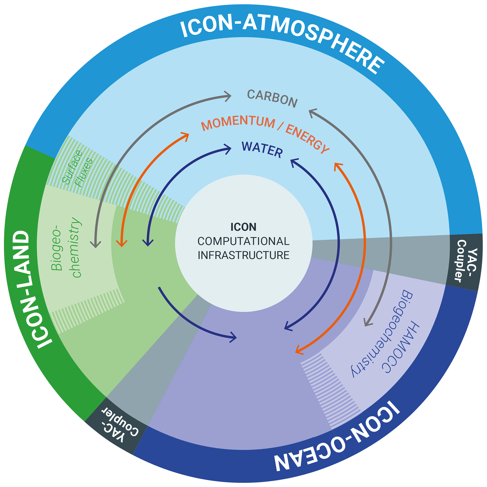
Figure 1Overview of the components of the ICON-Sapphire configuration with their interactions.
The ICON model was originally developed by the Max Planck Institute for Meteorology (MPI-M) for coarse-resolution (grid spacings of O(100 km)) climate simulations and by the German Weather Service (DWD) for weather forecasts. The DWD configuration, called ICON-NWP (Numerical Weather Prediction), only simulates the atmosphere together with a simple representation of land surface processes, whereas the MPI-M configuration includes all components traditionally used in ESMs, especially biogeochemistry on land and in the ocean. In the atmosphere, both model configurations share the same dynamical core and tracer transport scheme but rely on distinct physical parameterizations. The ICON dynamical core is based on the work of Gassmann and Herzog (2008) and Wan et al. (2013) (see Zängl et al., 2015), whereas the coarse-resolution climate configuration of ICON, called ICON-ESM, is presented in Jungclaus et al. (2022). Parallel to the development of this coarse-resolution configuration, MPI-M has developed its new Sapphire configuration, targeting grid spacings of 10 km and finer, including the ability to be used as a true ESM with interactive carbon on multi-decadal timescales.
As presented in more detail in the next sections, the Earth system in ICON-Sapphire is split into three main components: atmosphere, land, and ocean, with the ocean physical part including sea ice (see Fig. 1). Ocean biogeochemistry is simulated by the HAMburg Ocean Carbon Cycle (HAMOCC) model, whereas all land surface processes, including biogeochemistry, are simulated by the Jena Scheme for Biosphere–Atmosphere Coupling in Hamburg (JSBACH). Interactions between the atmosphere and the ocean are handled by the Yet Another Coupler (YAC), whereas, due to the choice of implicit coupling, the land is directly coupled to the atmosphere via the turbulence routine. The biogeochemical tracers in the ocean are transported by the same numerical routines as for temperature and salinity, and carbon is exchanged with the atmosphere. The atmosphere component of ICON-Sapphire can be run globally or on limited domains, both supporting only uniform grids (see Fig. 2). Higher resolution is achieved by nesting multiple simulations with successively finer grid spacings; these are simulations which communicate through the boundaries of their respective domains (see Sect. 4.2 for a practical example). The ocean component of ICON-Sapphire can only be run globally but can make use of a nonuniform grid, which allows smoothly refining the grid spacing in one simulation, thus zooming into a region of interest to achieve higher resolution.
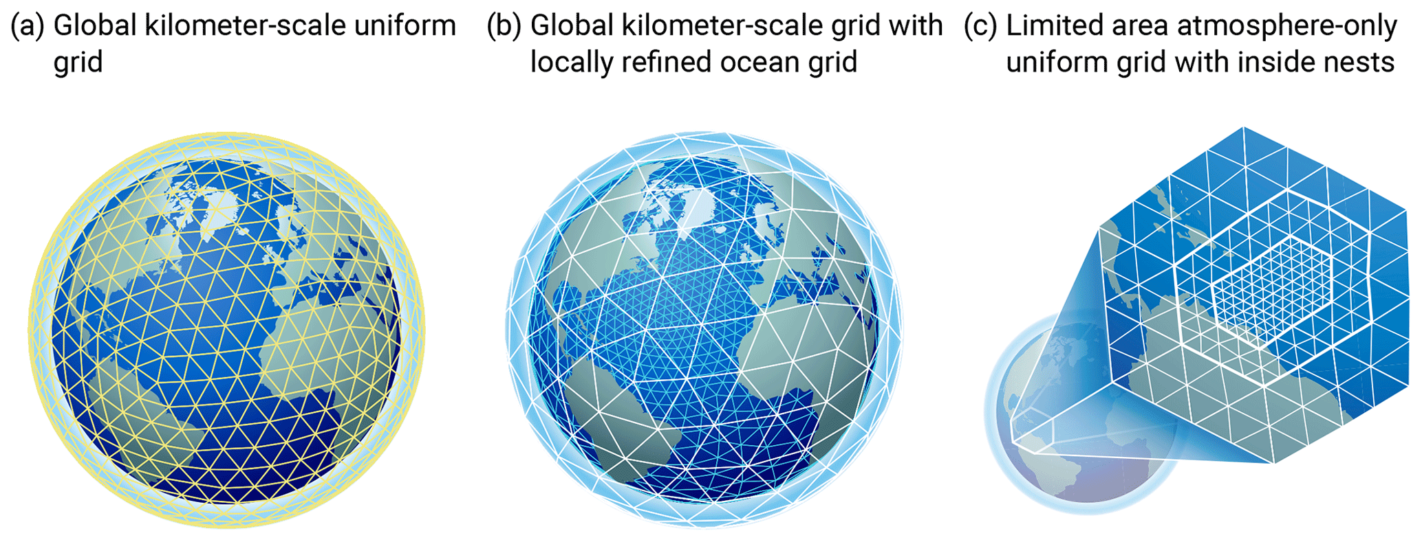
Figure 2Grid configurations supported by ICON-Sapphire: (a) global coupled kilometer-scale simulations with a uniform grid in the atmosphere and ocean, (b) global coupled kilometer-scale simulations with a uniform grid in the atmosphere and refined ocean grid over a specific region (telescope), with white for the atmosphere grid and blue for the ocean grid, and (c) atmosphere-only large eddy simulations over limited domains with the possibility of using inside nests to consecutively refine the resolution.
2.1 Atmosphere
The evolution of the atmosphere is simulated by solving the 3D nonhydrostatic version of the Navier–Stokes equations and conservation laws for mass and thermal energy on the sphere; see Eqs. (3)–(6) in Zängl et al. (2015). The equations are integrated in time with a two-time-level predictor–corrector scheme. Due to the presence of sound waves, the dynamics are sub-stepped so that dynamic adjustments happen at temporal increments 5 times smaller than physical adjustments, as schematically illustrated in Fig. 3. The spatial discretization is performed on an icosahedral–triangular C grid. On such a grid, the prognostic atmospheric variables are the horizontal velocity component normal to the triangle edges, the vertical wind component on cell faces, the virtual temperature, and the full air density including liquid and solid hydrometeors. The placing of these variables on the grid is illustrated in Fig. 4 of Giorgetta et al. (2018). The grid can be global or restricted to a limited area (see Fig. 2a, c). The limited-area implementation follows Reinert et al. (2022). The configuration uses a simple one-way or two-way nesting strategy at the boundary. Boundary conditions can be prescribed from larger-scale simulations (or reanalyses) or set to doubly periodic, as recently employed in Lee et al. (2022a) following Dipankar et al. (2015). In addition, there is the possibility to use inside nests. In this case, all the simulations are integrated at the same time but fine scales can be simulated over specific regions. In the vertical, a terrain-following hybrid sigma z coordinate (the Smooth LEvel VErtical coordinate, SLEVE) is used (Leuenberger et al., 2010) with a Rayleigh damping layer in the top levels after Klemp et al. (2008) using a Rayleigh damping coefficient of 1 s−1.
The ICON-Sapphire configuration only retains parameterizations for the physical processes, which unequivocally cannot be represented by the underlying equations at kilometer scales. Those are radiation, microphysics, and turbulence. It may be argued that other processes, like shallow convection, subgrid-scale cloud cover, and orographic drag, should still be parameterized at kilometer scales (Frassoni et al., 2018). We nevertheless refrain from including further or more complex parameterizations. First, it is especially important to have a slim code base that can be easily ported on emerging new computer architectures to fully exploit exascale computers given that the main roadblock preventing climate simulations at these fine grid spacings is computer resources (Palmer and Stevens, 2019; Schär et al., 2020). Second, parameterizations generally do not converge to a solution as the grid spacing is refined, unlike the basic model equations given appropriate discretization algorithms (Stevens and Lenschow, 2001). Along similar lines, underresolved processes at kilometer scales may look more similar to their resolved version than what a parameterization may predict. Hohenegger et al. (2020) showed that many large-scale bulk properties of the atmosphere, such as mean precipitation amount, already start to converge with a grid spacing of 5 km. Third, the need for parameterizations depends upon the intended use of the model. For a weather forecast model, it is important to simulate the atmospheric state as realistically as possible. In this sense, parameterizations may be viewed as a high-level way to tune a model. But this is not the goal of the developed ICON-Sapphire configuration, which is used as a tool to understand the Earth system and its susceptibility to change. In this context, the use of minimalistic physics also helps us understand which climate properties depend upon details of the flow that remain underresolved or parameterized at kilometer scales.
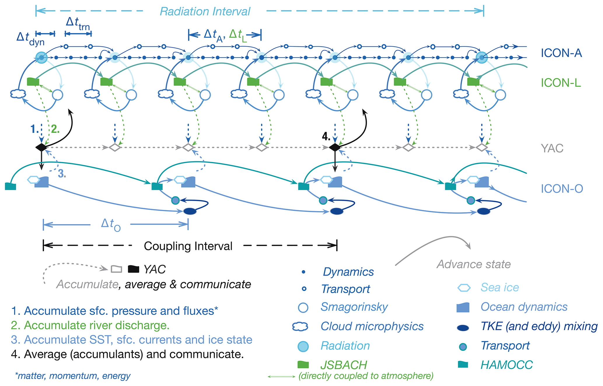
The calling order of the three parameterizations is illustrated in Fig. 3 together with the coupling between dynamics and physics. Radiation is parameterized by the Radiative Transfer for Energetics RRTM for General circulation model applications-Parallel (RTE-RRTMGP) scheme (Pincus et al., 2019). It uses the two-stream, plane-parallel method for solving the radiative transfer equations. The RRTMGP part of the scheme employs a k distribution for computing the optical properties based on profiles of temperature, pressure, and gas concentration. Gaseous constituents and aerosols are prescribed (see Sect. 2.5). The RTE part of the scheme then computes the radiative fluxes using the independent-column approximation in plane-parallel geometry. There are 16 bands in the longwave and 14 bands in the shortwave, and the spectrum is sampled using 16 g points per band. The RTE-RRTMGP scheme can be employed on both GPU and CPU architectures, unlike its predecessor PSrad (Pincus and Stevens, 2013). All simulations presented in this study were nevertheless performed with PSrad as, at first, the RTE-RRTMGP scheme was unexpectedly slow on CPUs. This issue has now been solved and all future simulations with ICON-Sapphire will employ RTE-RRTMGP. Differences between the two schemes are the use of a more recent spectroscopy and roughly twice as many g points in RTE-RRTMGP, although a version with a reduced number of g points, similar to the one used with PSrad, exists for RTE-RRTMGP as well. Due to the high computational cost of radiation schemes in general, radiation is called less frequently than the other parameterizations (see Fig. 3).
For the parameterization of microphysical processes, two schemes employed in the ICON-NWP configuration have been implemented in ICON-Sapphire. There is the option to choose between a one-moment (Baldauf et al., 2011) and a two-moment (Seifert and Beheng, 2006) scheme. All the simulations of this study were conducted using the one-moment scheme. The one-moment scheme predicts the specific mass of water vapor, cloud water, rain, cloud ice, snow, and graupel. In addition, the two-moment scheme predicts the specific numbers of all hydrometeors and also includes hail as one supplementary hydrometeor category. Saturation adjustment is called twice, before and after calling the microphysical scheme. All hydrometeors (number and mass) are advected by the dynamics, but only cloud water and ice are mixed by the turbulence scheme and are optically active. Condensation requires the full grid box to be saturated. ICON-Sapphire does not use a parameterization for subgrid-scale clouds, leading to a binary cloud cover of 0 or 1 at each grid point.
Turbulence is handled by the Smagorinsky scheme (Smagorinsky, 1963) with modifications by Lilly (1962). The implementation and validation of the Smagorinsky scheme are described in Lee et al. (2022a), following Dipankar et al. (2015). The Smagorinsky scheme is the scheme of reference for parameterizing turbulence in large eddy simulations as it includes horizontal turbulent mixing. Strictly speaking, it was not designed for applications at kilometer scales as it assumes that most of the turbulent eddies can be represented explicitly by the flow (e.g., Bryan et al., 2003). It has nevertheless been successfully used with kilometer grid spacings in both idealized and realistically configured simulations (e.g., Klemp and Wilhelmson, 1978; Langhans et al., 2012; Bretherton and Khairoutdinov, 2015). The surface fluxes are computed according to Louis (1979) using the necessary information provided by the land surface scheme; see Sect. 2.2 for a description of the coupling between the land surface and the atmosphere.
2.2 Land
Land processes are simulated by the JSBACH land surface model version 4. It provides the lower boundary conditions for the atmosphere over land, namely albedo, roughness length, and the necessary parameters to compute latent and sensible heat fluxes from similarity theory. The latter are part of solving the surface energy balance equation, which is, together with the multi-soil thermal layers, implicitly coupled to the atmospheric diffusion equations for vertical turbulent transport following the Richtmyer and Morton numerical scheme (Richtmyer and Morton, 1967). A multi-layer soil hydrology scheme is used for the prognostic computation of soil water storage (Hagemann and Stacke, 2015). Surface runoff and subsurface drainage are collected in rivers and are routed into the ocean by the hydrological discharge model of Hagemann and Dümenil (1997) with river directions determined by the steepest descent (Riddick, 2021). The physical, biogeophysical, and biogeochemical processes included in JSBACH are described in Reick et al. (2021) for JSBACH version 3.2. These processes are leaf phenology, dynamical vegetation, photosynthesis, carbon and nitrogen cycles, natural disturbances of vegetation by wind and fires, and natural and anthropogenic land cover change. New features in JSBACH 4 are the inclusion of freezing and melting of water in the soil, a multi-layer snow scheme (Ekici et al., 2014; de Vrese et al., 2021), and the possibility to compute the soil properties as a function of the soil water and organic matter content. Land surface processes are called at the same time as the main atmospheric processes (see Fig. 3) and integrated on the same grid. From an infrastructure point of view, JSBACH 4 has been newly designed in a Fortran 2008 object-oriented, modular, and flexible way.
Given the targeted horizontal resolution of ICON-Sapphire, there is no subgrid-scale heterogeneity in vegetation type. Only one vegetated tile is used, characterized by a vegetation ratio that gives the area coverage of vegetation over that tile, implicitly accounting for the presence of bare soil on the vegetated tile. A land cell can nevertheless be split between lake and vegetated or be fully covered by a glacier. Lakes are fractional but are not allowed in coastal cells. The surface temperature of lakes is computed by a simple mixed layer scheme including ice and snow on lakes (Roeckner et al., 2003). In coastal regions, fractional land is permitted.
In this study, JSBACH has been used in a simplified configuration that only interactively simulates the physical land surface processes, as in weather forecasts or in traditional general circulation models. Leaf phenology is prescribed following a monthly climatology. Interactive leaf phenology has been employed in Lee et al. (2022a) with idealized radiative convective equilibrium simulation conducted using a grid spacing of 2.5 km. Also, the hydrological discharge model was turned off. Initialization of the hydrological discharge model reservoirs using remapped values taken from a prior MPI-ESM simulation failed. With this approach, unrealistically large discharge values occurred during the first 3 months, indicative of a poor initialization. Moreover, the discharge of a river is dumped into the uppermost ocean layer in a single cell, which is an unrealistic assumption with kilometer grid spacings. By running an offline version of the hydrological model to quasi-equilibrium to obtain better initial states of the reservoirs and by redistributing the discharge over multiple ocean cells, the mentioned problems could be solved. Newer simulations conducted with ICON-Sapphire include river discharge.
2.3 Ocean
The ocean model ICON-O (see Korn, 2018; Korn et al., 2022) solves the hydrostatic Boussinesq equations, the classical set of dynamical equations for global ocean dynamics. The time stepping is performed using a semi-implicit Adams–Bashforth-2 scheme in which the dynamics of the free surface are discretized implicitly. ICON-O evolves the state vector consisting of the horizontal velocity normal to the triangle edges, surface elevation, potential temperature, and salinity. The UNESCO-80 formulation is employed as equation of state to compute density given potential temperature, salinity, and depth. ICON-O uses, as the atmosphere, an icosahedral–triangular C grid. However, in contrast to the atmosphere, the global grid can be locally refined to create a “computational telescope” (Fig. 2b) that zooms into a region of interest. The numerics of ICON-O share similarities to the atmosphere component but also have important differences. Both components use a mimetic discretization of discrete differential operators, but ICON-O uses the novel concept of Hilbert-space compatible reconstructions to calculate volume and tracer fluxes on the staggered ICON grid (see Korn, 2018). The transport of the oceanic tracers potential temperature and salinity is performed using a flux-corrected transport scheme with a Zalesak limiter and a piecewise-parabolic reconstruction in the vertical direction, analogous to what is done for the atmospheric tracers. The numerical scheme of ICON-O allows for generalized vertical coordinates: of particular importance here are the depth-based z and z* coordinates. In the z-coordinate system, only the sea surface height varies in time. Since the surface height is added to the thickness of the top grid cell, the combination of a thin surface grid cell with a strong reduction of sea surface height can lead to a negative layer thickness, creating a model blow-up. This problem is avoided by using the z* coordinate. In this case, the changing domain of the ocean is mapped onto a fixed domain but with vertical coordinate surfaces that change in time. For the simulations presented in this study, the z coordinate was used.
Given the fine resolution of ICON-Sapphire, only a subset of the parameterizations available in ICON-O and described in detail in Sect. 2.2 of Korn et al. (2022) are used, namely a parameterization for vertical turbulent mixing and one for velocity dissipation. The parameterization of turbulent vertical mixing relies on a prognostic equation for turbulent kinetic energy and implements the closure suggested by Gaspar et al. (1990), wherein a mixing length approach for the vertical mixing coefficient for velocity and oceanic tracers is used. For velocity dissipation (or friction), either a “harmonic” Laplace, a “biharmonic” iterated Laplace operator, or a combination of the two can be used. The viscosity parameter can be set to a constant value, scaled by geometric grid quantities such as edge length of triangular area, or computed in a flow-dependent fashion following the modified Leith closure in which the viscosity is determined from the modulus of vorticity and the modulus of divergence (Fox-Kemper and Menemenlis, 2008). The calling order between dynamics, physics, and transport is illustrated in Fig. 3.
The sea ice model is part of ICON-O. It consists of a dynamic and a thermodynamic component. Sea ice thermodynamics describe freezing and melting by a single-category, zero-layer formulation (Semtner, 1976). The current sea ice dynamics are based on the sea ice dynamics component of the Finite-Element Sea Ice Model (FESIM) (Danilov et al., 2015). The sea ice model solves the momentum equation for sea ice with an elastic–viscous–plastic (EVP) rheology. The configuration of the sea ice model with an EVP rheology and single-category instead of multi-category sea ice thermodynamics was chosen because of computational efficiency considerations. Recent work (e.g., Wang et al., 2016) suggests that the EVP rheology provides at a high resolution of 4.5 km a good compromise between physical realism and computational efficiency. Since ICON-O and FESIM use different variable staggering, a wrapper is needed to transfer variables between the ICON-O grid and the sea ice dynamics component (see Korn et al., 2022). A new sea ice dynamics model has been developed to bypass these limitations (see Mehlmann et al., 2021; Mehlmann and Korn, 2021) and will be employed in the future.
The ocean biogeochemistry component is provided by HAMOCC6 (Ilyina et al., 2013). It simulates at least 20 biogeochemical tracers in the water column, following an extended nutrient, phytoplankton, zooplankton, and detritus approach, also including dissolved organic matter, as described in Six and Maier-Reimer (1996). It also simulates the upper sediment by 12 biologically active layers and a burial layer to represent the dissolution and decomposition of inorganic and organic matter as well as the diffusion of pore water constituents. The co-limiting nutrients consist of phosphate, nitrate, silicate, and iron. A fixed stoichiometry for all organic compounds is assumed. Phytoplankton is represented by bulk phytoplankton and diazotrophs (nitrogen fixers). Particulate organic matter (POM) is produced by zooplankton grazing on bulk phytoplankton and enters the detritus pool. Export production is separated explicitly into CaCO3 and opal particles. The POM sinking speed is calculated using the Microstructure, Multiscale, Mechanistic, Marine Aggregates in the Global Ocean (M4AGO) scheme (Maerz et al., 2020). The time stepping and horizontal grid are as in ICON-O.
2.4 Coupling
For the coupling between the atmosphere and the ocean (see Figs. 1 and 3), we use YAC (Hanke et al., 2016) version 2.4.2. This version has been completely rewritten. In particular, each MPI process now only has to provide its own local data to the coupler without any information about MPI processes containing neighboring partitions of the horizontal grid. Furthermore, the internal workload is now evenly distributed among all source and target MPI processes.
The atmosphere provides to the ocean the zonal and meridional components of the wind stress separately over ocean and sea ice given their different drag coefficients, the surface freshwater flux as rain and snow over the whole grid cell, and evaporation over the ocean fraction of the cell, shortwave and longwave radiation, latent and sensible heat fluxes over the ocean, sea ice surface and bottom melt potentials, the 10 m wind speed, and sea level pressure. The ocean provides the sea surface temperature, the zonal and meridional components of velocity at the sea surface, the ice and snow thickness, and ice concentration. The interpolation of the wind is done using the simple one-nearest-neighbor method when the grid of the ocean and of the atmosphere matches. For more complex geometries, the wind is interpolated using Bernstein–Bézier polynomials following Liu and Schumaker (1996). We use the so-called interpolation stack technique of YAC and apply a four-nearest-neighbor interpolation to fill target cells with incomplete Bernstein–Bézier interpolation stencils. All other fields are interpolated with a first-order conservative remapping. The land–sea mask is determined by the ocean grid. The coupler and our coupling strategy are designed to conserve fluxes.
2.5 Input/output
External data and initial conditions are interpolated onto the horizontal grid at a preprocessing step. Vertical interpolation is done online during the model simulation. Concerning the land surface, required external physical parameters are based on the same data set (Hagemann, 2002; Hagemann and Stacke, 2015) as used in the past in the MPI-ESM (Mauritsen et al., 2019). These data sets have an original grid spacing of 0.5∘ × 0.5∘. For experiments at kilometer scales, this is not optimal and work to derive these parameters directly from high-resolution data sets is underway. The orography is nevertheless derived from the Global Land One-km Base Elevation Project (GLOBE), which has a nominal resolution of 30′′, so about 1 km. Likewise, the bathymetry has a 30′′ resolution, as provided by the Shuttle Radar Topography Mission (SRTM30_PLUS) data set (Becker et al., 2009). In the atmosphere, for the simulations presented in this study, global mean concentrations of greenhouse gases are set to their values of the simulated year, with values taken from Meinshausen et al. (2017). Ozone varies spatially on a monthly timescale. The data set is taken from the input data sets for model intercomparison projects (input4MIPS) with a resolution of 1.875∘ by 2.5∘ (latxlon), and the year 2014 is chosen as default. Aerosols are specified from the climatology of Kinne (2019), which provides monthly data on a 1∘ grid.
Initial conditions for the atmosphere are derived from the European Centre for Medium-Range Weather Forecasts (ECMWF) operational analysis for the chosen start date. Initial conditions for soil moisture, soil and surface temperatures, and snow cover are also derived from the ECMWF analysis. The soil is not spun up as it is unclear how to best do this in global climate storm-resolving simulations. Analysis of the output of the global coupled 5 km simulation nevertheless reveals that four of the five soil layers are already equilibrated after 7 simulation months in the northern extratropics, defined from 30 to 60∘ N, and three of them in the tropics in the sense that the continuous drying of the soil since simulation start has stopped. In contrast, all the ocean prognostic variables are spun up. The ocean initial state is taken from a spun-up ocean model run with climatological forcing. As the spin-up methodology slightly differs between the different experiments presented in this study, it is described for each simulation individually in more detail in Sect. 4 where the simulation results are presented.
ICON-Sapphire uses asynchronous parallel input/output because efficient parallel I/O is the main performance bottleneck. Moreover, the size of a single 3D variable is too big to fit into the memory of one CPU. The model calculations are carried out in parallel and the output is distributed across the local memories of the cluster's CPUs. The employed approach is to hide the overhead introduced by the output behind the computation (“I/O forwarding”). By using dedicated I/O processes, the simulations can be further integrated in time while dedicated CPUs handle the I/O. Moreover, reading and writing files in parallel greatly reduces the time spent on I/O (see Sect. 3).
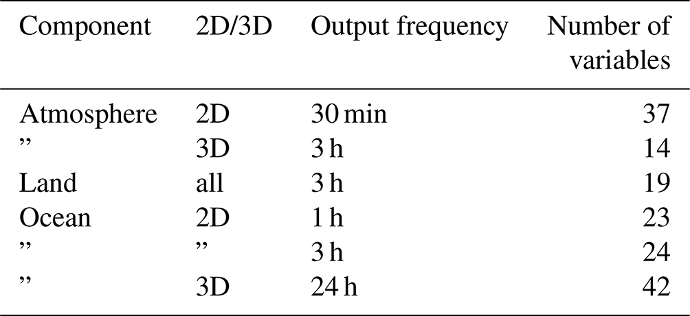
One challenge of kilometer-scale simulations is the amount of output generated. At 2.5 km, the atmosphere contains 83 886 080 cells at each of the 90 vertical levels of our set-up, and the ocean contains 59 359 799 cells and 112 levels. The output has mostly been analyzed using Jupyter notebooks and Python, with which efficient ways to analyze the output directly on the unstructured grid have been developed. As part of ICON-Sapphire activities and of the next Generation Earth Modelling Systems (nextGEMS) project, an e-book has been developed as a community effort, providing information on the simulations as well as hints and example scripts. The e-book can be found at https://easy.gems.dkrz.de (last access: 17 January 2023). An important tool for selecting a subset of the output or in general for reformatting and transforming variables is the Climate Data Operators (CDO), which are developed at MPI-M (Schulzweida, 2022). Calculations are performed in CDO with double precision, whereas the output format of ICON-Sapphire simulations (see next section) is single precision. To reduce the memory requirement, single-precision 32 bit data are now mapped directly in memory without conversion. This reduces the memory requirement for memory-intensive operations by a factor of 2. New operators have also been created to support unstructured grids, e.g., selcircle, selregion, maskregion, and sellonlatbox; see the latest release of the CDO documentation for more information (Schulzweida, 2022).
Table 1 focuses on the performance of the global coupled simulations conducted with ICON-Sapphire as those are the type of simulations that ultimately should be integrated on multi-decadal timescales, and Table 2 summarizes the type of variables outputted for one simulation. In ICON terminology (Giorgetta et al., 2018), the considered grid spacings are R2B9 and R2B10, which approximately correspond to grid spacings of 5 and 2.5 km, respectively. Note that on the unstructured ICON grid, all cells have approximately the same area, and the grid spacing in kilometers corresponds to the square root of the mean cell area. The specific settings of the simulations are summarized in Table 3 and described in more detail in the next section when we present the simulation results. For the 5 km simulation, we write about 40 TB of output per month (uncompressed) using NetCDF-4 and 32 bit as output format. The output storage increases to 135 TB per month for the 2.5 km simulation, making it clear that new output strategies have to be developed for longer-term simulations.
The production simulations have been performed on the supercomputer Levante of the German Climate Computing Center (DKRZ). Levante was ranked 86 in the top 500 list in November 2021 (time of installation) and replaced the previous machine Mistral. Table 1 indicates that ICON-Sapphire scales very well with node number. Increasing the node number by a factor of 6, from 100 to 600 nodes, leads to a factor of 5.25 increase in simulated days per day (SDPD) for the simulation with 5 km grid spacing on Levante. The scaling starts breaking when using more than 400 nodes. Going from the old machine Mistral to the new machine Levante leads to a 5.6× increase in SDPD for the same number of nodes. There are two reasons for this increase. From a technical point of view, we expect a gain in throughput by roughly a factor of 4 from the increase in the number of processors per node (128 on Levante versus 32 on Mistral). The additional gain is attributed to a more economic use of resources due to the introduction of asynchronous ocean output, which became available only recently.
Making use of these various advantages, Table 1 reveals that a throughput of 126 SDPD is achieved on Levante for a grid spacing of 5 km when using 600 nodes, or 21 % of the compute partition. This is slightly larger than the minimum throughput of 100 SDPD considered to be needed for climate simulations to be useful (see introduction). With a grid spacing of 2.5 km, a throughput of 20 SDPD is obtained on 600 nodes. On the one hand, it is slightly better than the theoretically expected 8-fold decrease in performance due to the doubling in grid spacing. On the other hand, it is presently still too small to allow conducting climate simulations at such a high resolution. At best, a throughput of 100 SDPD would be obtained if using the whole Levante and assuming a perfect scaling.
Instead of CPUs, GPUs can be used to obtain a better throughput. GPUs are available on the supercomputer JUWELS Booster at the Jülich Supercomputing Centre. One JUWELS Booster node is about 0.05 PFlops compared to 0.003 PFlops for one Levante node in terms of their linpack benchmarks. Hence, in theory, we would expect a performance increase of 17 going from Levante to JUWELS Booster, giving a throughput of almost 1SYPD for the 2.5 km configuration. Giorgetta et al. (2022) compared atmosphere-only 5 km simulations conducted with ICON on JUWELS Booster (with GPU) and on Levante (with CPU) using a slightly different model configuration than our ICON-Sapphire set-up, consisting of a different turbulence scheme and using RTE-RRTMGP as radiation scheme. In their study, the performance increase is closer to 8 (see their Table 3). This would mean that 1 SYPD would be feasible on a 68 PFlops machine, a machine 1.5 times the size of JUWELS Booster. Such a throughput would now be possible on petascale machines such as Europe's most powerful supercomputer LUMI in Finland with 150 PFlops. GPUs are interesting not only because of their performance increase but also because of their low energy consumption. JUWELS Booster gets about 50 PFlops per MW, whereas Levante gets about 4.6 PFlops per MW. So even if JUWELS Booster is less productive than expected from the number of PFlops per node, it still does 5 times as much throughput per watt than Levante.
A grid spacing of 1.25 km (R2B11) is the highest grid spacing that has currently been tested with the coupled ICON-Sapphire configuration. It has been integrated for 5 d, with a throughput of 2.5 SDPD (see Table 1). This number could be improved by a better load balancing between the ocean and atmosphere as currently the ocean waits upon the atmosphere. The atmosphere-only version of ICON-Sapphire has been run at 1.25 km on Levante on 908 nodes for 3 d, giving a throughput of 4 SDPD. Also, an ocean-only version of ICON-Sapphire has been run at 1.25 km on Levante. The throughput is 97 SDPD on 1024 nodes and 179 SDPD on 2048 nodes, which is 15 % short of the expected perfect scaling (194 SDPD on 2048 nodes). These numbers indicate that the ocean also begins to become a bottleneck to reach 1 SYPD with a grid spacing of 1.25 km. Although these numbers are by far too low to allow multi-decadal simulations, even on a machine like LUMI, seasonal timescales are in principle already possible on a global scale and with a grid spacing of 1.25 km using ICON-Sapphire.
Table 1Performance of global coupled configuration runs with a grid spacing of 5 and 2.5 km, called G_AO_5km and G_AO_2.5km in Table 3 summarizing the setting of all simulations, and with a grid spacing of 1.25 km. The performance at 1.25 km is also given for an atmosphere-only (A) and ocean-only (O) configuration as the throughput of the coupled simulation has not been fully optimized yet. Under nodes, “A” stands for atmosphere and “O” for ocean. On Levante, the A and O numbers give the load balancing, and on Mistral they directly give the number of processors. The specifications of Mistral and Levante nodes are as follows. Mistral node: 2x 18-core Intel Xeon E5-2695 v4 (Broadwell) 2.1GHz, connected with Fourteen Data Rate (FDR) Infiniband; Levante node: 2x AMD 7763 CPU; 128 cores.
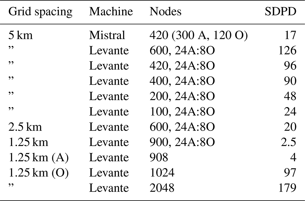
Table 2Overview of the output of the simulation with a grid spacing of 5 km, called G_AO_5km in Table 3.
In this section, we present key examples of simulations conducted with ICON-Sapphire to illustrate its intended abilities. The simulation settings are summarized in Table 3. As will be shown, the simulated fields agree to a satisfactory degree with expectations and observations, even though we identify aspects of the climate system that remain problematic to capture and would require further tuning of ICON-Sapphire for improvement. In addition, the versatility and good scalability of ICON-Sapphire allow its use in a variety of set-ups at the forefront of exascale climate computing. Extrapolating from these results, ICON-Sapphire now allows Earth system simulations with interactive carbon with a grid spacing of 10 km for multi-decadal timescales. At the other end of the spectrum, ICON-Sapphire allows studying the effects of submesoscale eddies in the ocean by employing its telescope feature and large eddies in the atmosphere by employing its limited-area ability on the transport of energy and matter.
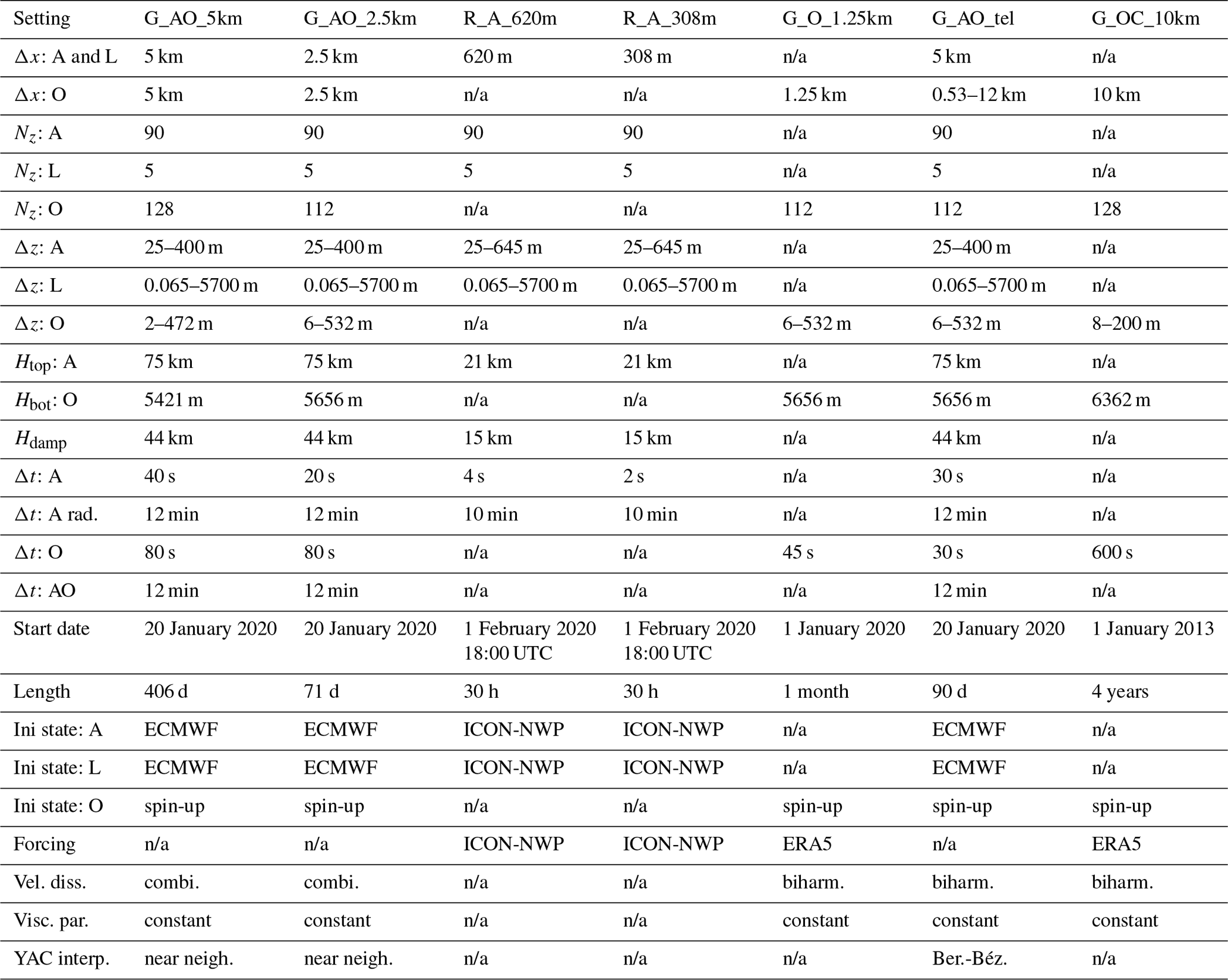
Table 3Summary of simulation settings. More information on the employed external data is in Sect. 2.5 and on the ocean spin-up in Sect. 4 in the respective subsections. Abbreviations A, L, O, and C are for atmosphere, land, ocean, and carbon; n/a is for not applicable, Δx for the horizontal grid spacing, Δz for the vertical grid spacing, Nz for the number of vertical levels, Htop for the domain top, Hbot for the ocean bottom, Hdamp for the height at which damping starts in the atmosphere, and Δt for the time step. Note that in the atmosphere and on land, Δz increases with height, which is not the case in the ocean where the top layer has a thickness of 7 m. “Forcing” indicates the simulation providing the lateral boundary conditions in the limited-area atmosphere-only simulations and the simulation providing the atmospheric forcing in the ocean-only simulations. Given the strong vertical stretching in the upper atmosphere, the indicated Δz in the atmosphere is for layers below 14 km.
4.1 Simulating the coupled ocean–atmosphere system globally on seasonal timescales at 5 and 2.5 km
In this section, we present results from global coupled simulations conducted with ICON-Sapphire employing a uniform grid spacing of 5 and 2.5 km, referred to as G_AO_5km and G_AO_2.5km for global atmosphere–ocean simulation with the suffix indicating the grid spacing (see Table 3 and Fig. 2a). The length of the simulation periods is unique, with G_AO_5km integrated for more than 1 year from 20 January 2020 to 28 February 2021 and G_AO_2.5km for 72 d from 20 January 2020 to 30 April 2020 to at least cover the time period of the new winter DYAMOND intercomparison study. The necessary initial and external data are listed in Sect. 2.5. The ocean is spun up by conducting an ocean-only simulation. We start with a grid spacing of 10 km and use the Polar science center Hydrographic Climatology 3.0 (PHC) observational data set (Steele et al., 2001) to initialize all ocean fields. That simulation is run for 1 year 25 times using the Ocean Model Intercomparison Project (OMIP) atmospheric forcing by Röske (2006). Then the simulation is forced from 1948 to 1999 by the National Centers for Environmental Prediction (NCEP) reanalysis (Kalnay et al., 1996) and from 2000 to 2009 by the ECMWF reanalysis ERA5 (Hersbach et al., 2020). The obtained state serves as a new initial state for a 5 km ocean-only simulation forced by ERA5 and integrated over the time period 2010 to 20 January 2020. This end state is interpolated onto the 2.5 km grid to obtain the initial state of G_AO_2.5km. In all the simulations, sea surface salinity is relaxed towards observed 10 m salinity of the PHC data set with a time constant of 3 months. Through this initialization technique, the ocean is spun up and already entails mesoscale eddies without having to use a multi-decadal spin-up at 2.5 km, which is computationally too expensive. The conducted long spin-up gives some confidence that the ocean model is working correctly. Comparing the last full month of the spin-up (December 2019) to the Ocean Reanalysis System 5 (ORAS5, Zuo et al., 2019), the global mean SST bias is −0.53 K. The SST is consistently too cold except along 60∘ S, north of 50∘ N, and along the western coast of North America. Due to the relaxation, the salinity is well captured except in the Arctic Ocean, with the latter showing a bias of more than 1 g kg−1.
Despite the uniqueness of the integration period for such simulations, the shortness of the integration period makes it challenging to validate the simulations as we cannot expect to reproduce one particular observation year. As such, we will not only consider the mean climatology from observations, but include year-to-year variability in the analysis. Also, the integration period remains too short to demonstrate at the outset that the ocean model works correctly given its slow dynamics. As a consequence, we will focus the ocean validation on variables that couple more strongly to the atmosphere and react fast. The ocean validation merely intends to show that no obvious bias exists, as for many scientific questions, e.g., related to the seasonal migration of tropical rain belts, effects of instability waves on air–sea fluxes, or interactions between ocean, atmosphere, and ice as shown in some of the examples below, an integration period of 1 year is sufficient. Despite the long experience of running ICON at low resolution in a coupled mode (Jungclaus et al., 2022), it is not a given that the ocean works and couples correctly to the atmosphere. In fact, several bugs were discovered during the development phase of the coupled high-resolution configuration, in particular bugs related to the momentum coupling between the ocean and atmosphere.
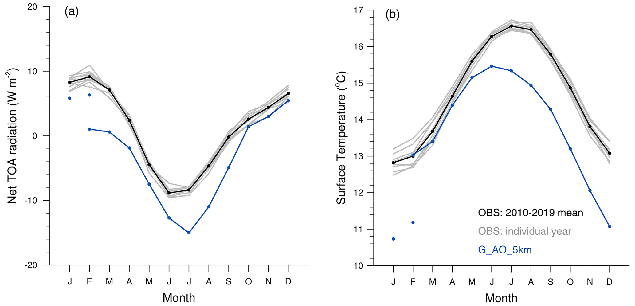
Figure 4Seasonal cycle in (a) net TOA radiation and (b) surface temperature from observations and G_AO_5km. Observations in (a) are from CERES-EBAF (Clouds and the Earth's Radiant Energy System–Energy Balanced and Filled, Loeb et al., 2018) version 4.1 with a grid spacing of 1∘ and in (b) from HadCRUT (Hadley Centre/Climatic Research Unit Temperature, Morice et al., 2021) version 5.0 with a grid spacing of 5∘. For G_AO_5km, the solid marked line shows the months in 2020 and the two dots in 2021.
4.1.1 5 km results
As ESMs aim to represent the flow of energy and matter in the Earth system, we start our validation with energy. Figure 4a displays the seasonal cycle in the net top-of-the-atmosphere (TOA) energy. Too much energy leaves the Earth system in G_AO_5km during the first half of the year, by 3 to more than 6 W m−2 compared to observations. The simulation adjusts with time and better matches the observations from September 2020 to February 2021 with a remaining underestimation between 1 and 3 W m−2. Overall, this leads to a yearly imbalance of −4 W m−2 in G_AO_5km. This imbalance results from an overly high reflection of shortwave radiation by 7.3 W m−2, which is partly compensated for by corresponding outgoing longwave radiation that is too weak by 3.3 W m−2. The bias in shortwave radiation is due to too much reflection over oceans (11 W m−2), whereas the land shows too little reflection (by 3.7 W m−2). The differences are especially prominent over tropical oceans in regions of shallow convection and stratocumulus, which exhibit cloud cover that is too large (not shown). This is expected from storm-resolving simulations whose grid spacings remain too coarse to properly resolve shallow convection (e.g., Hohenegger et al., 2020; Stevens et al., 2020a). The consequence is a spurious and strong increase in cloud cover the coarser the grid spacing is. In contrast, the bias in outgoing longwave radiation is more prominent over the extratropics, especially over the Northern Hemisphere extratropics, with a deviation of 6 W m−2 against 3 W m−2 in the Southern Hemisphere extratropics and 2 W m−2 in the tropics. The simulated outgoing longwave radiation that is too weak is in agreement with the Northern Hemisphere extratropics being much colder (and cloudier) than observations, a reflection of their larger land fraction (see further below).
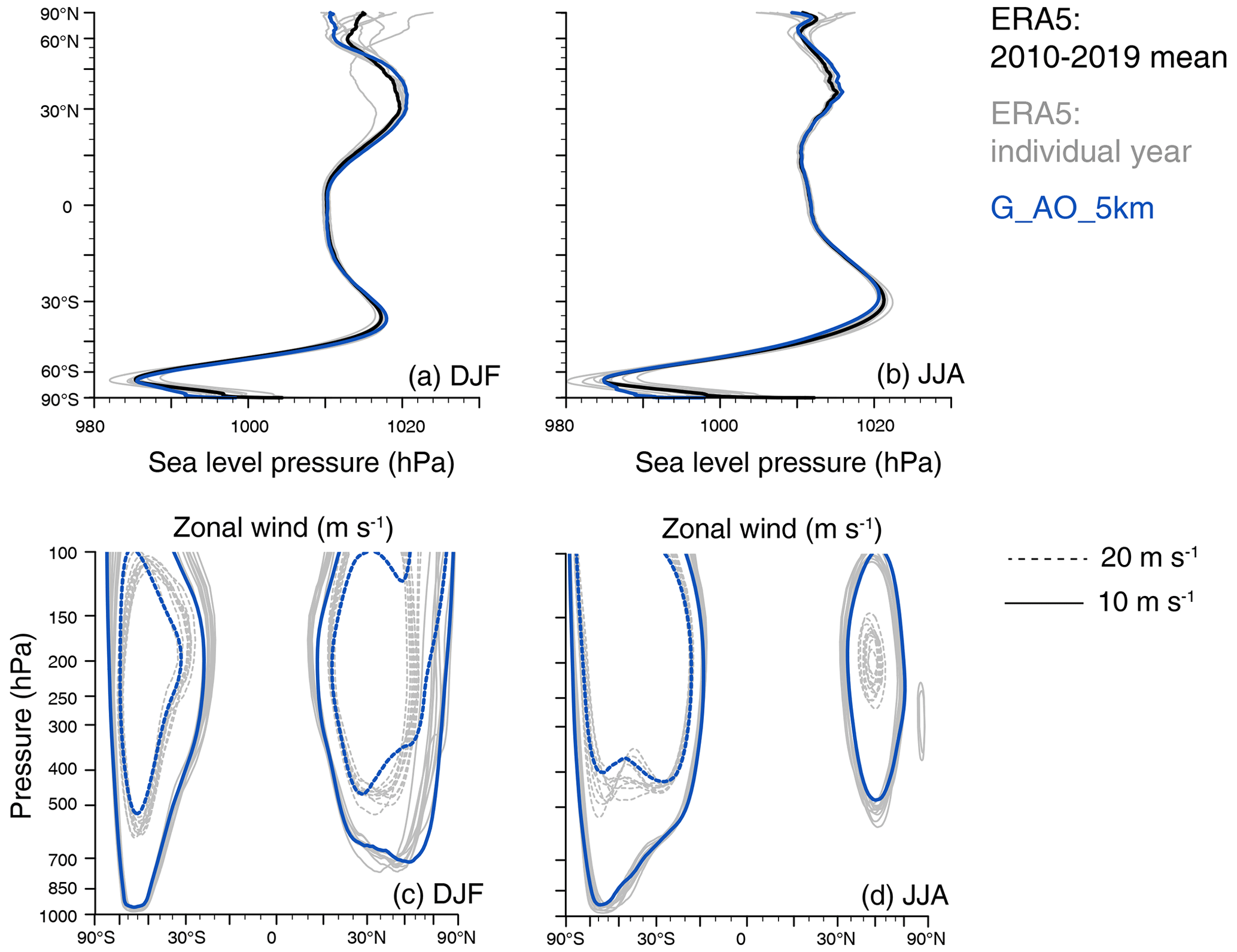
Figure 5Meridional cross-sections of zonally averaged sea level pressure (hPa) for (a) DJF and (b) JJA as well as height–latitude cross-sections of zonal wind velocity (m s−1) for (c) DJA and (d) JJA from ERA5 (grid spacing of 30 km) and G_AO_5km. In G_AO_5km, DJF is the mean from December 2020 to February 2021.
As explained in Mauritsen et al. (2012), it is common practice in ESMs to tune the radiation balance to adjust uncertain parameters related to unresolved processes. Given the obtained yearly imbalance of −4 W m−2, this need to adjust parameter values remains true at 5 km. However, known tuning knobs of coarse-resolution simulations, such as entrainment rates of convective parameterizations or cloud inhomogeneity parameters, either do not exist anymore or were not as efficient as at low resolution. A promising route to tune the TOA imbalance in ICON-Sapphire, which is currently under investigation, is to slightly adapt the mixing formulation in the Smagorinsky scheme. Our current formulation sets the eddy diffusivities to zero if the Richardson number is greater than the eddy Prandtl number. This cutoff unrealistically inhibits mixing because of well-known limitations of the Smagorinsky scheme in simulating the transition to turbulence (Porte-Agel et al., 2000) and because of a failure to incorporate the effect of moist processes. As a result, over cold and moist surfaces, insufficient ventilation of the boundary layer occurs, causing moisture to build up and resulting in excessive low clouds. In ongoing experiments, we have explored adding a small amount of background mixing at interfaces between saturated and unsaturated layers where the equivalent potential temperature decreases upward, mimicking the effects of buoyancy reversal (Mellado, 2017). Low clouds respond sensitively to this background mixing. Adapting the amount of this background mixing provides a convenient tuning knob on the quantity of low clouds and their influence on the top-of-the-atmosphere energy budget.
Complicating the issue, several areas where energy is not conserved have been identified: the dynamical core unphysically extracts energy from the flow at a rate of about 8 W m−2, and precipitation is an unphysical source of energy. The former has been documented by Gassmann (2013). The latter arises because hydrometeors are assumed to have the temperature of the cell in which they are found. Because this assumption neglects the cooling of the air that accompanies the precipitation through a stratified atmosphere, it acts as an internal energy source of roughly (and coincidentally) equal magnitude as the dynamic sink. This explains why these energy leaks, which are also present in ICON-ESM, were not discovered previously. Moreover, minor energy leaks related to phase changes in the constant volume grid not conserving internal energy, as well as to an inconsistent formulation of the turbulent fluxes, have been discovered. Fixes for all of these problems have been identified and are being implemented.
Given that the Earth system is losing too much energy, a cooling of the global mean surface temperature is expected (Fig. 4b). The mean values are 286.5 K in G_AO_5km against 287.9 K in observations. Biases are stronger over land than over oceans, with a mean bias of −1.7 K over land versus −0.6 K over oceans, likely reflecting the smaller heat capacity of the land surface (see also Fig. 5f in Mauritsen et al., 2022, for an overview of the spatial distribution of temperature biases during JJA).
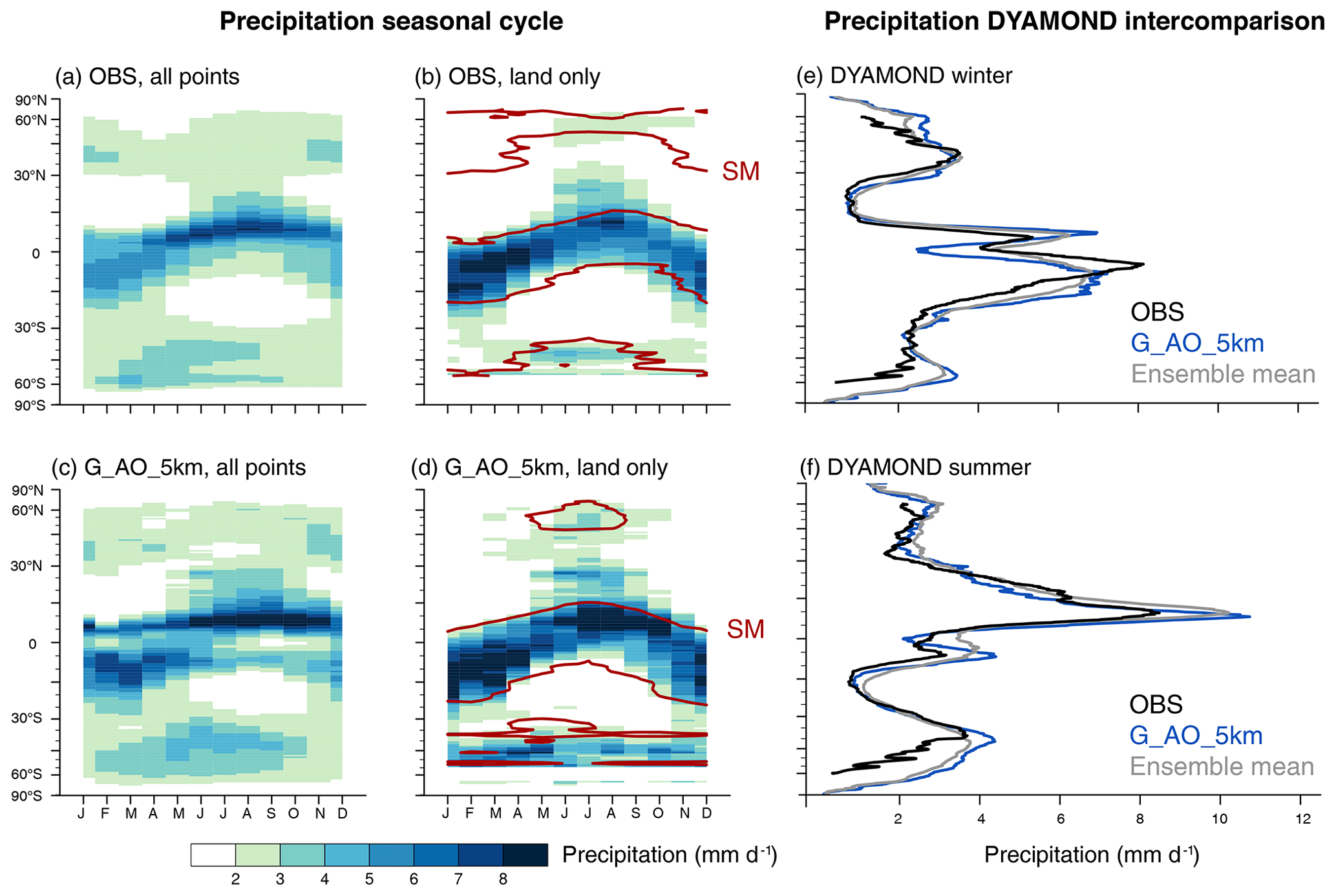
Figure 6Seasonal evolution of zonal mean precipitation (shading) from (a–b) observations and (c–d) G_AO_5km. In panels (b) and (d), only land points are included with the soil moisture (SM) contour overlaid in brown (1.5 cm in b and 1 cm in d given their distinct magnitude). Observations are from the Global Precipitation Climatology Project (GPCP, grid spacing of 2.5∘, Adler et al., 2018) and from the European Space Agency Climate Change Initiative (ESACCI, Dorigo et al., 2017) soil moisture (grid spacing of 0.25∘) averaged over the years 2010–2019. For G_AO_5km the January and February values are from 2021. Panels (e)–(f) show the zonal mean precipitation from (e) the DYAMOND winter and (f) DYAMOND summer intercomparison study including the ensemble mean of participating models.
ICON-Sapphire explicitly represents the modes of energy transport. In the atmosphere, storms (baroclinic eddies) dominate the energy transport in the extratropics, whereas atmospheric convection dominates the vertical energy transport in the tropics. We thus now investigate the representation of the large-scale circulation and precipitation. Figure 5a and b show meridional cross-sections of zonally averaged sea level pressure in G_AO_5km and reanalysis for winter and summer. Except for sea level pressure over Antarctica that is too low, the simulated sea level pressure lies within the internal variability from the reanalysis. The location and strength of the midlatitude low-pressure systems and of the subtropical high-pressure systems match ERA5, and their expected seasonal migration and intensification is reproduced. Similarly good agreement is obtained by looking at the jets (see Fig. 5c–d). Both the location and intensity of the jet in the winter hemisphere lie within internal variability. The position of the jet in the summer hemisphere is also well captured, but the simulated jet is weaker than the jet in the reanalysis, consistently so in the Northern Hemisphere.
Figure 6 shows the observed and simulated seasonal cycle in precipitation. The bands of enhanced precipitation within the extratropical storm tracks can be recognized together with their seasonal cycle. Averaged over the midlatitudes, defined from 30∘ poleward, precipitation amounts to 2.37 mm d−1 in G_AO_5km against 2.31 mm d−1 for the 10-year observational mean and is larger than any of the observed yearly mean values by at least 0.03 mm d−1. Likewise, the migration of the tropical rain belt is generally captured in the zonal mean (see Fig. 6a and c), although the Equator stands out in G_AO_5km with too little precipitation. This leads to the formation of a double Intertropical Convergence Zone (ITCZ) over the western Pacific with two parallel precipitation bands; the southern band is too zonal, reaching too far east and remaining south of the Equator even during boreal summer (see Fig. 6a and c). This bias is linked to SSTs that are too low at the Equator, as shown in Segura et al. (2022) in their detailed assessment of the representation of tropical precipitation in G_AO_5km. Over land (Fig. 6b and d), in contrast, the seasonal migration of the tropical rain belt is very well reproduced, but the amounts are overestimated. Tropical mean precipitation amounts over land are 3.6 mm d−1 in G_AO_5km and 3.11 mm d−1 in observations for the 10-year mean, with no observed yearly value larger than 3.30 mm d−1.
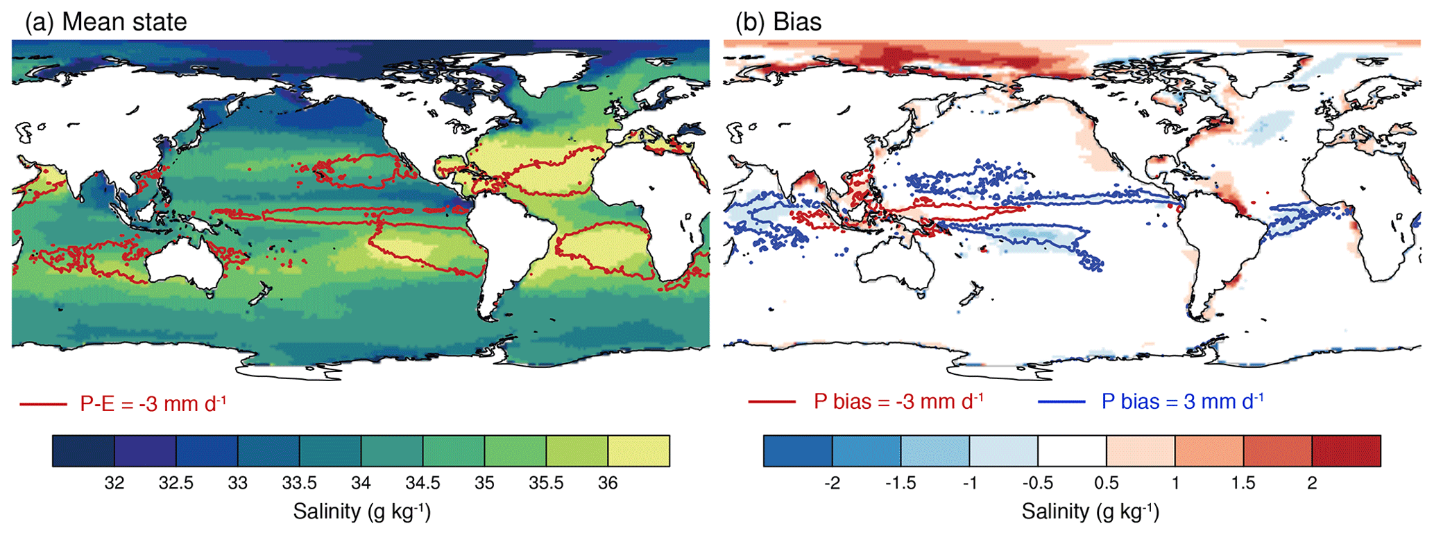
Figure 7Salinity (g kg−1) from G_AO_5km as (a) a temporal mean and (b) bias relative to observations overlaid with contour lines representing P−E in (a) and precipitation bias in (b). Observations from PHC (grid spacing of 1∘) for salinity and from GPCP for precipitation. For G_AO_5km, the time period 1 March 2020 to 28 February 2021 is considered.
Hence, ICON-Sapphire overestimates precipitation amounts at least over the tropics. This remains true in the global mean, with an overestimation by 0.4 mm d−1. The overestimation is indicative of a radiative cooling of the atmosphere that is too strong. However, even on the observational side, existing discrepancies between observed net radiation and observed precipitation suggest that precipitation amounts may in reality be larger than what observational precipitation data sets are suggesting (Stephens et al., 2012). Despite these apparent discrepancies, the simulated precipitation is close to the mean precipitation as derived from the ensemble of storm-resolving models participating in the DYAMOND intercomparison study, as shown in Fig. 6e and f. As the DYAMOND models employ prescribed SST derived from ECMWF analysis, the good agreement gives us confidence in the behavior of G_AO_5km. The most noticeable difference, which is clearly out of the ensemble mean, is the underestimation of precipitation at the Equator during DYAMOND winter.
Explicitly representing convection is important not only for explicitly representing one of the main modes of energy transport in the tropics but also for explicitly simulating the transport of water that is important for the biosphere. The brown contour line in Fig. 6b and d depicts the seasonal cycle in soil moisture. Not surprisingly, in the tropics, it matches the migration of the tropical rain belt very well, as also found in observations. In the northern extratropics, the moistening of the soil during summertime seems consistent with the simulated enhanced precipitation, but is inconsistent with observations. This inconsistency may be related to the difficulty of measuring soil moisture during winter due to the presence of ice and snow. In any case, the hydrological budget over land is closed in ICON-Sapphire. As a second main discrepancy, soil moisture is consistently lower in G_AO_5km than in observations and gets drier with time.
The effect of precipitation on the ocean is investigated by comparing salinity and precipitation minus evaporation (P−E) patterns as a sanity check (Fig. 7a). As expected, P−E imprints itself on salinity to a first order (Fig. 7a). Areas with evaporation much stronger than precipitation are more salty. Biases in salinity are small with values smaller than 0.5 g kg−1 except in the western Arctic (Fig. 7b). The latter bias was already present in the spin-up. Interestingly, and even though we are comparing climatological to yearly values and observations from different sources, there seems to be a good correlation in the tropics between precipitation biases and salinity biases, especially in areas receiving too much precipitation. Positive localized salinity biases can also be recognized at the mouth of big rivers, like the Amazon, the Mississippi, or the Congo, which is a signature of not having freshwater discharge into the salty ocean (see Sect. 2.2). Being related to the absence of river discharge and to the simulated precipitation pattern, the pattern of the salinity bias in the tropics is distinct from the one at the end of the spin-up period.
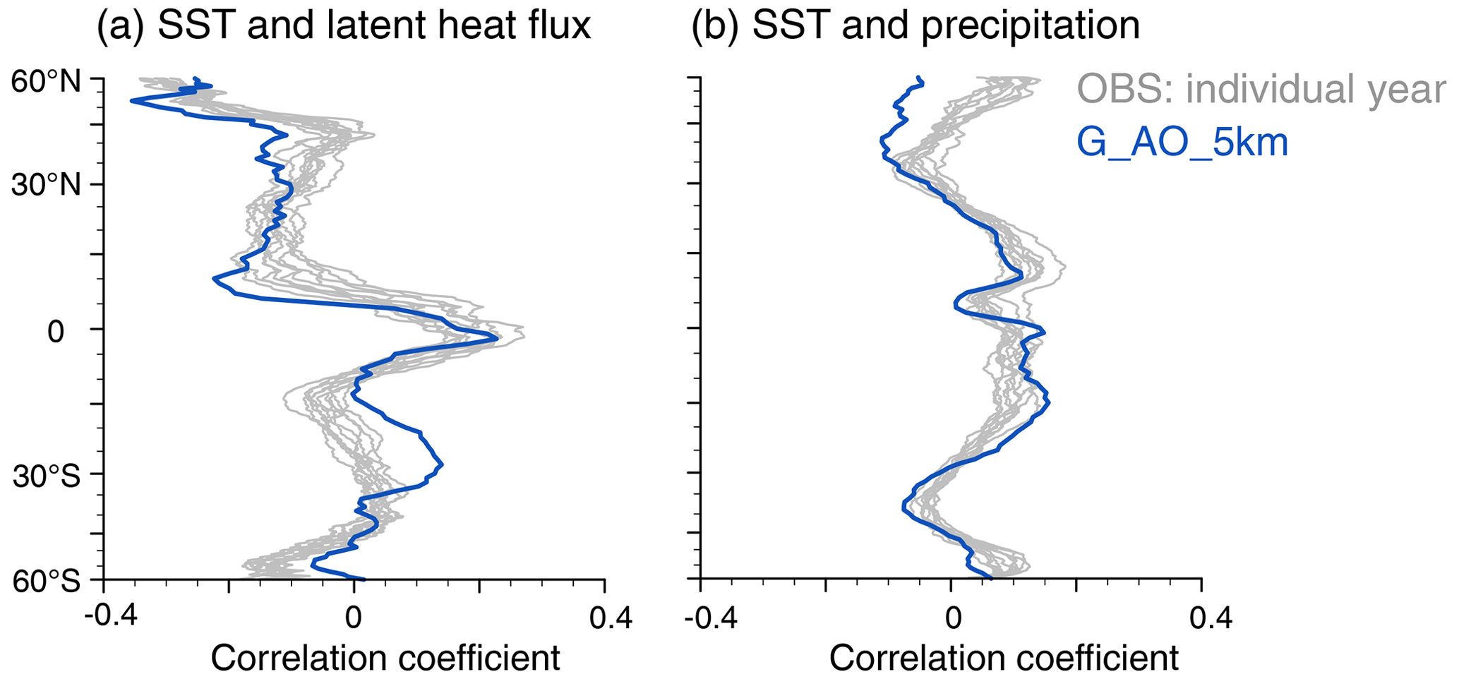
Figure 8Meridional cross-section of zonally averaged correlation between SST and (a) latent heat flux and between SST and (b) precipitation. Observed SST from the Optimum Interpolation SST (OISST, grid spacing 0.25∘, Reynolds et al., 2018), latent heat flux from the Objectively Analyzed air–sea flux (OAFlux_V3, grid spacing 1∘), and precipitation from the Integrated Multi-satellitE Retrievals for Global Precipitation Measurement (IMERG, grid spacing 0.1∘). Daily values are used.
The coupling between the ocean and the atmosphere is further investigated in Fig. 8 by computing correlations between SST, latent heat flux, and precipitation at each grid point and averaging these values zonally. As shown in Wu et al. (2006), the investigated coarse-resolution climate model simulations struggle to capture basic features of air–sea interactions, with an especially widespread positive correlation between SST and precipitation, whereas observations show clear meridional differences in the correlation between SST and precipitation (see their Fig. 3). As shown by Fig. 8, G_AO_5km reproduces the order of magnitude of the correlation as well as its meridional variations between SST and latent heat flux and between SST and precipitation. The main bias is a positive correlation between SST and latent heat flux in the Southern Hemisphere subtropics, which is at odds with the observed negative correlation. Concerning precipitation, even though the strength of the simulated coupling between SST and precipitation is within observed individual years, it tends to fall either on the weak or on the strong side. The exception is in the higher northern latitudes that have a negative correlation between SST and precipitation, which is opposite to the positive correlation seen in observations.
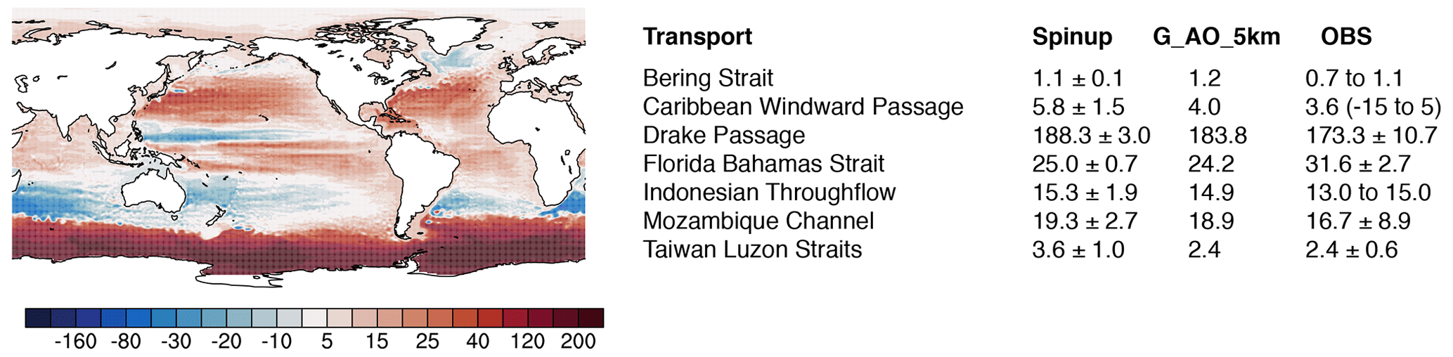
Figure 9Barotropic streamfunction (Sv) with associated major transports that can be computed from the streamfunction. Observations for the historic period are taken from Table J2 of Griffies et al. (2016) except for the Drake Passage, which is taken from a more recent estimate (Donohue et al., 2016). In the table, the spin-up values are averaged over the years 2015–2021 with 1 standard deviation indicated.
The dynamical coupling between the atmosphere and the ocean is reflected in the wind-driven circulation, which responds fairly fast when coupling the ocean component to the atmosphere component. This circulation is described by the barotropic streamfunction (see Fig. 9) with positive values indicating clockwise flows. G_AO_5km simulates the main features of the wind-driven circulation: the subtropical and subpolar gyres in the North Atlantic and the strong circumpolar currents in the Southern Ocean. When considering the mass transports through major transects, the simulated transports compare reasonably well with those found in observations. Compared to the mean transport obtained in the spin-up, the transport, with the exception of the Bering Strait, is weaker, with values out of 1 standard deviation for all the passages but the Indonesian Throughflow and the Mozambique Channel. Except for the Florida–Bahamas strait, the weaker transport of G_AO_5km is in better agreement with observations. The weaker transport is consistent with weaker wind stress in G_AO_5km compared to the spin-up simulation, also expressed in a weaker barotropic streamfunction (not shown).
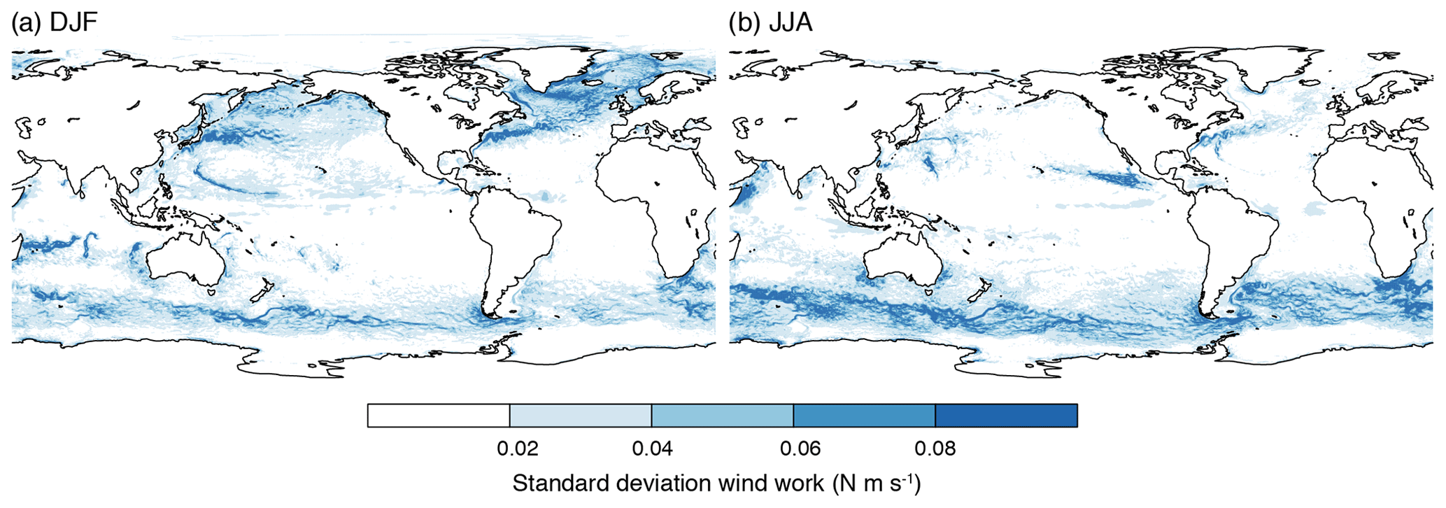
Figure 10Standard deviation of wind work in G_AO_5km based on daily values for (a) DJF and (b) JJA.
The dynamical coupling between the atmosphere and the ocean is also reflected in the variability of wind work (Fig. 10), which is defined as the product of surface wind stress and surface ocean currents (Wunsch, 1998). In eddy-rich regions such as the Gulf Stream, the Kuroshio current, the Agulhas Return Current, the Brazil–Malvinas confluence, and the Southern Ocean, strong dynamic interaction is seen year-round and is stronger in their respective winter hemisphere. The shift in direction associated with monsoonal winds induces the seasonal (boreal summer) Great Whirl off the Somali coast that is also associated with pronounced ocean–atmosphere interactions, which may affect the Indian summer monsoon (Seo, 2017). While this has been simulated in a regional coupled model (Seo et al., 2007), global storm-resolving configurations like G_AO_5km enable us to investigate even larger-scale effects. Tropical cyclone tracks are also visible, for instance off the coast of Central America in the eastern Pacific in JJA. The total wind work displayed by Fig. 10 is 3.21 TW. In comparison, Flexas et al. (2019) estimated 4.22 TW for their ∘ simulation.

Figure 11(a–c) Composite diurnal cycle of the upper-ocean daily temperature anomaly in G_AO_5km as well as in observations with associated net heat flux at the ocean surface. Observations are from ship data for the net heat flux and from three Slocum gliders for the temperature. Observations and G_AO_5km are averaged between 57–58∘ W and 11.5–14.∘ N and from 21 January–29 February 2020. Panel (d) shows meridional cross-sections of wind together with meridional variations in SST and precipitation in (e) from G_AO_5km averaged over February 2020 through the central–eastern Pacific ITCZ. Panels (f)–(g) are like panels (d)–(e) but over the Gulf Stream. In (g) the SST Equator-to-pole meridional gradient is removed. Zonal averages are taken between 150 and 90∘ W in (d)–(e) and between 60 and 20∘ W in (f)–(g).

Figure 12A low-pressure system in the Southern Ocean and associated large- and small-scale features, visualized from G_AO_2.5km with (a) salinity, (b) salinity (shading) and sea level pressure (contour lines), (c) wind (streamlines) and surface temperature (shading), (d) wind (streamlines) and ocean velocity (shading), (e) wind (streamlines) and rain (blue shading), and (f) wind (streamline), rain (blue), and cloud (white). The field of view is towards the Bay of Bengal. The tip of India and Sri Lanka can be recognized.
As a final illustration of the coupling between the ocean and the atmosphere, which, for the first time, may not be blurred by the use of a convective parameterization, we show in Fig. 11 three examples taken from different regimes: a subsiding subtropical region coincident with the area of operation of the EUREC4A (ElUcidating the RolE of Clouds–Circulation Coupling in Climate) field campaign (Stevens et al., 2021), a region of deep convection with the Pacific Intertropical Convergence Zone (ITCZ), and the Gulf Stream, the latter motivated by the findings of Minobe et al. (2008). G_AO_5km reproduces the observed diurnal cycle of net heat flux and temperature very well (Fig. 11a, b, c). The onset of ocean cooling and warming phases around 21:00 and 11:00 local time as well as the development of a diurnal warm layer during daytime are well represented in G_AO_5km compared to the observed data. We nevertheless note that the simulated surface warming and cooling do not propagate far enough into the ocean, potentially pointing to too little mixing. Ocean-only simulations conducted at a grid spacing of 5 km indeed reveal a strong sensitivity of the mixed layer depth to the chosen mixing parameter in the turbulent kinetic energy (TKE) mixing scheme, with mixed layers that are generally too shallow over the tropical Atlantic. The cross-section through the ITCZ (Fig. 11d, e) reveals features that can hardly be reproduced with coarse-resolution ESMs: a narrow region of about 5∘ of strong ascent around 6∘ N with associated boundary layer wind convergence and upper-level divergence at the top of the deep convection at around 300 hPa. Precipitation peaks below the convergence, a region which coincides with high SST and strong SST gradients, which are two features favorable for the development of deep convection. Figure 11e also reveals the previously mentioned low SSTs and dip in precipitation at the Equator. Finally, the atmospheric cross-section taken over the Gulf Stream (Fig. 11f, g) also reveals enhanced precipitation under the area of strong vertical motion. The latter sits on the top of the warm water of the Gulf Stream, albeit slightly shifted northward, blending with the jet location.
4.1.2 2.5 km results
The global ocean–atmosphere coupled simulation with a grid spacing of 2.5 km (G_AO_2.5km) employs the same set-up as G_AO_5km, except for its finer grid spacing and, accordingly, reduced time step, as well as for a slightly distinct arrangement of the vertical levels in the ocean (see Table 3). We now show four examples illustrating small-scale features embedded in larger-scale structures that such a model configuration aims to resolve. We also chose the four examples to illustrate interactions involving different components of the Earth system, which is rendered possible with the design of ICON-Sapphire.
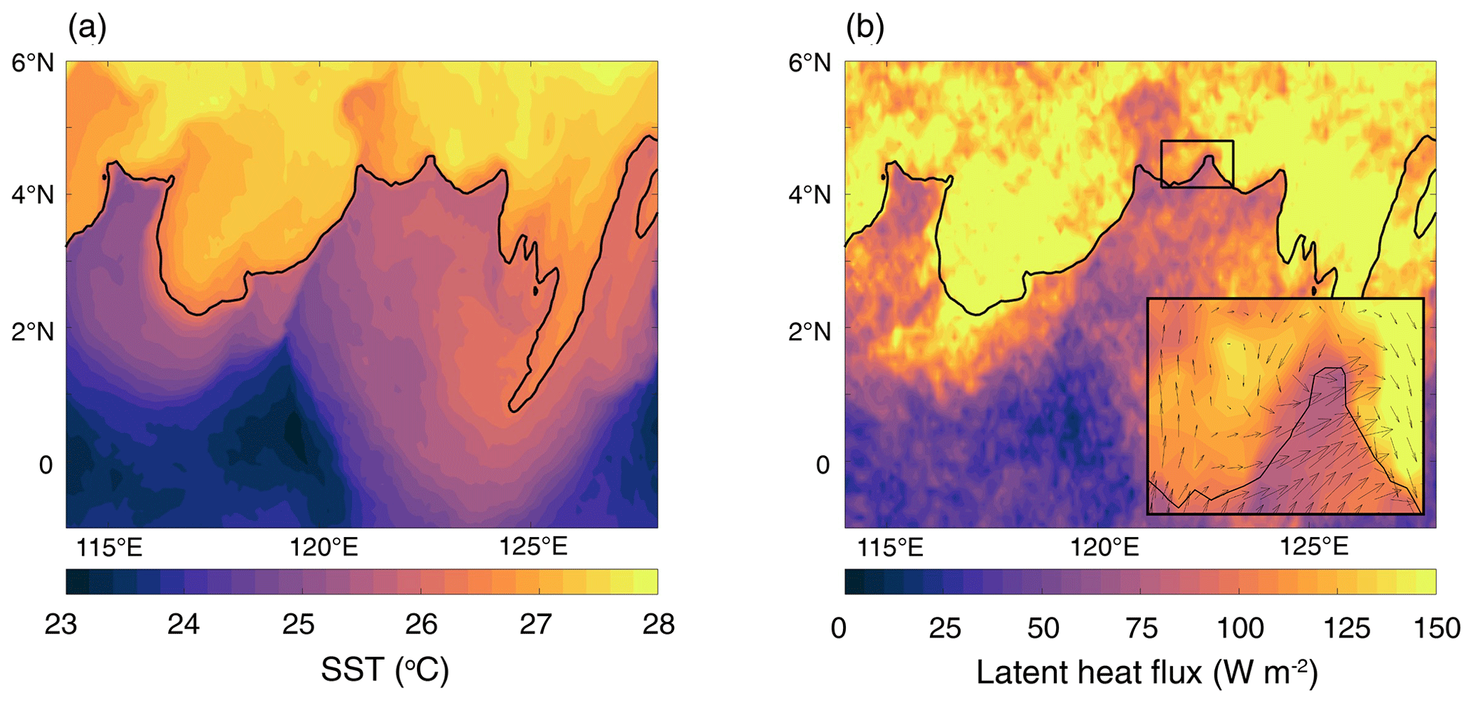
Figure 13Breaking of a tropical instability wave in the Pacific in G_AO_2.5km with (a) SST and (b) latent heat flux. The black line shows the 26.3∘C isoline. Snapshot for 5 February 2020 at 23:00. The inset in (b) shows a blow-up of the region enclosed by the rectangle at about 4∘ N and 122∘E.
Figure 12 focuses on the Southern Ocean. On the small scale, ocean eddies and filaments of enhanced velocity (Fig. 12d) imprint themselves on the salinity (Fig. 12a) and SST (Fig. 12c) fields, as expected. Superimposed on this variability, on the large scale, cold and salty water encounters warm and fresh water, leading to the formation of a large-scale SST front. At this front, a low-pressure system (Fig. 12b) develops with its associated circling wind (shown as streamlines), precipitation, and clouds (Fig. 12e, f). But even in this large-scale low-pressure system, the precipitation is neither randomly nor uniformly distributed but aligns with the circling streamlines, forming mesoscale bands of precipitation. Comparing Fig. 12c and f, perhaps surprisingly, a cooling of the surface below clouds and a freshening of the ocean below precipitation are not noticeable.
Figure 13 illustrates the breaking of tropical instability waves. Tropical instability waves already develop in ocean models with a grid spacing of 0.25∘ (Jochum et al., 2005); the finer grid spacing nevertheless allows resolving the submesoscale structure along the wave cusps with the development of secondary fronts. These secondary fronts rotate counterclockwise, while the tropical instability waves break clockwise. The imprint of these secondary fronts in the surface flux, as shown in Fig. 13b for latent heat, is noteworthy.
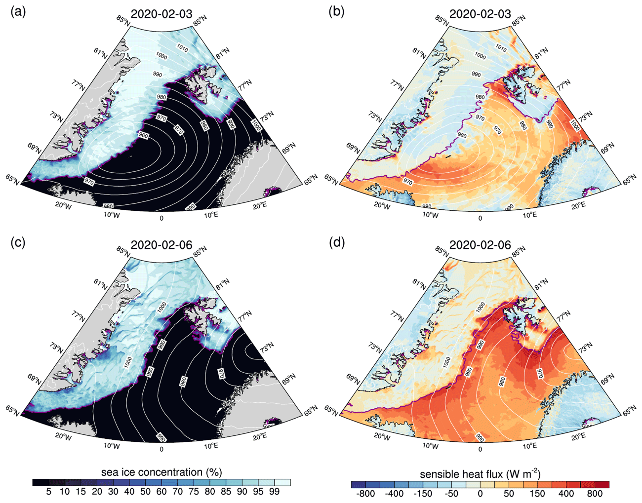
Figure 14Sea ice breakup by a polar low and the effect on sensible heat flux in G_AO_2.5km. Daily mean values are shown. The white contour lines are for sea level pressure (hPa), and the magenta line is for the extent of the sea ice (15 % concentration).
In Fig. 14, the interactions between the ocean, sea ice, and atmosphere are illustrated. The passage of a polar low leads to the formation of narrow leads a few kilometers wide and polynyas; compare Fig. 14c after the passage and Fig. 14a before the passage. The sea ice breakup results from the strong wind stress exerted by the southerly winds on the back of the polar low. By resolving these small-scale linear kinematic features in the sea ice, heat is released from leads and polynyas, whereas there is no or negative heat flux over thicker ice (compare Fig. 14c and d). Positive heat fluxes over leads and polynyas are to be expected and have been measured, for example, during the Surface Heat Budget of the Arctic Ocean (SHEBA) field experiment (Overland et al., 2000). Using a development version of ICON-Sapphire run at 5 km, Gutjahr et al. (2022) also illustrated the interactions between the polar low, katabatic storms, and dense water formation in the Irminger Sea.
Lastly, as expected for such a resolution, G_AO_2.5km can resolve mesoscale circulations induced by surface heterogeneity, which is most easily seen over islands, and their impacts on convection (not shown).
4.2 Resolving large eddies in the atmosphere
Simulations like G_AO_5km and G_AO_2.5km enable studies of the effect of small scales, in particular those associated with deep convection and ocean mesoscale eddies, on the large-scale transport of matter and energy in the ocean–atmosphere system. On the atmosphere side, such grid spacings are unable to represent the effects of yet smaller scales, such as those associated with boundary layer turbulence or non-precipitating convection. A poor representation of non-precipitating clouds may lead to biases in solar radiation, as documented in the previous section. Large eddies in the atmosphere can be resolved with ICON-Sapphire by using its limited-area and nesting capabilities (Fig. 2c), combined with hectometer and decameter grid spacings, as shown with the help of one example in this section. We keep the presentation short as it is now well established that large eddies in the atmosphere can be resolved on limited domains with hectometer and decameter grid spacings (e.g., Stevens et al., 2020a).
To demonstrate that ICON-Sapphire can be conducted over a limited area with an inside nest for local refinement, we present the results of such a configuration (see Fig. 15 and Table 3). The chosen grid spacings are 620 m (R2B12) and 308 m (R2B13) for the outer and inner nests. The resulting two simulations are referred to as R_A_620m and R_A_308m for regional atmosphere-only simulations with the grid spacing as a suffix. The simulation domain extends over the subtropical western Atlantic, encompassing Barbados, to match the domain of operation of the EUREC4A field campaign (Stevens et al., 2021). It covers the area between 60–50∘ W and 10–16∘ N in R_A_620m and between 59.9–56∘ W and 12–14.5∘N in R_A_308m. The simulations start 1 February 2020 at 18:00 UTC and are integrated until 3 February at 00:00 UTC. We chose to simulate 2 February as that day shows different patterns of mesoscale cloud organization (Narenpitak et al., 2021). During the simulation period, the cloud field transitions from one form of mesoscale organization (Sugar) to another one (Flowers, following the terminology introduced by Stevens et al., 2020b). The initial state and lateral boundary conditions are derived from a limited-area simulation conducted with the ICON-NWP model covering a large part of the tropical Atlantic, between 67–43∘ W and 0–24∘N, and using a grid spacing of 1.25 km. The lateral boundary conditions are read in every hour and two-way nesting is employed.
Figure 15 shows a snapshot of liquid water path and provides visual evidence of mesoscale organization of the cloud field in observations and as reproduced in the two simulations. The observed cloud field is organized in separated clusters (Flowers) on the western half of the domain and in more fine-grained patterns (Sugar) in the eastern half of the domain with equally spaced lines. This organization is well reproduced by R_A_620m, and even the spacing between the Sugar lines seems to be similar to the observed one. Flowers are also simulated by R_A_308m. In both simulations, the cloud pattern seems more spotty than in observations. Averaged over the EUREC4A circle of flight operation, centered at 13.3∘ N, 57.717∘ W with a diameter of 220 km, and during the 8 h flight time on 2 February, the cloud cover amounts to 0.18 in R_A_620m and 0.17 in R_A_308m. In comparison, Konow et al. (2021) reported values between 0.1 and 0.2 from five out of six instruments with the mean cloud cover of these five instruments around 0.15, which is close to the simulated values. Overall this indicates that large eddy simulations with ICON-Sapphire can be conducted for regional climate or process studies.
Figure 15Snapshot of liquid water path on 2 February 2020 at 13:00 UTC from (a) observations, (b) R_AO_620m, and (c) R_AO_308m. Observations are from the Pathfinder ATMOSpheres (PATMOS) derived from GOES (grid spacing of 1 km).
4.3 Resolving submesoscale eddies in the ocean
Not only in the atmosphere, but also in the ocean, ICON-Sapphire makes use of grid spacings at kilometer scales and below to allow for submesoscale dynamics. This capability is demonstrated by presenting the results of two types of simulations (see Table 3). One is a global ocean-only simulation with a grid spacing of 1.25 km, referred to as G_O_1.25km. In the second type, the horizontal grid is refined up to 530 m to create a “computational telescope” (Fig. 2b) that zooms into the North Atlantic, while the grid becomes increasingly coarser outside this region down to 12 km. The latter configuration, referred to as G_AO_tel, is run coupled to an atmosphere. The atmosphere employs a grid spacing of 5 km and the same settings and parameterizations as G_AO_5km. We choose the North Atlantic as a focal region and started the simulation in boreal winter because of the favorable conditions for submesoscale dynamics.
The initial ocean state for the two simulations is obtained as follows. We branch off on 1 October 2019 from the 5 km ocean-only simulation that was used to spin up G_AO_5km (see Sect. 4.1). That state is interpolated on a 2.5 km grid and run until 1 January 2020, providing the initial state for both G_O_1.25km and an ocean-only simulation using the same setting as G_AO_tel. After 20 d, the atmosphere is coupled to the ocean in the latter case.
Figure 16 shows the details of the dynamics that can be simulated with a grid spacing of 1.25 km through a snapshot of kinetic energy. In particular in the Northern Hemisphere, structures are visible that have spatial scales smaller than the first baroclinic deformation radius. The Southern Hemisphere shows fewer of these structures, what can be expected since submesoscale dynamics are thought to decrease during local summer conditions.
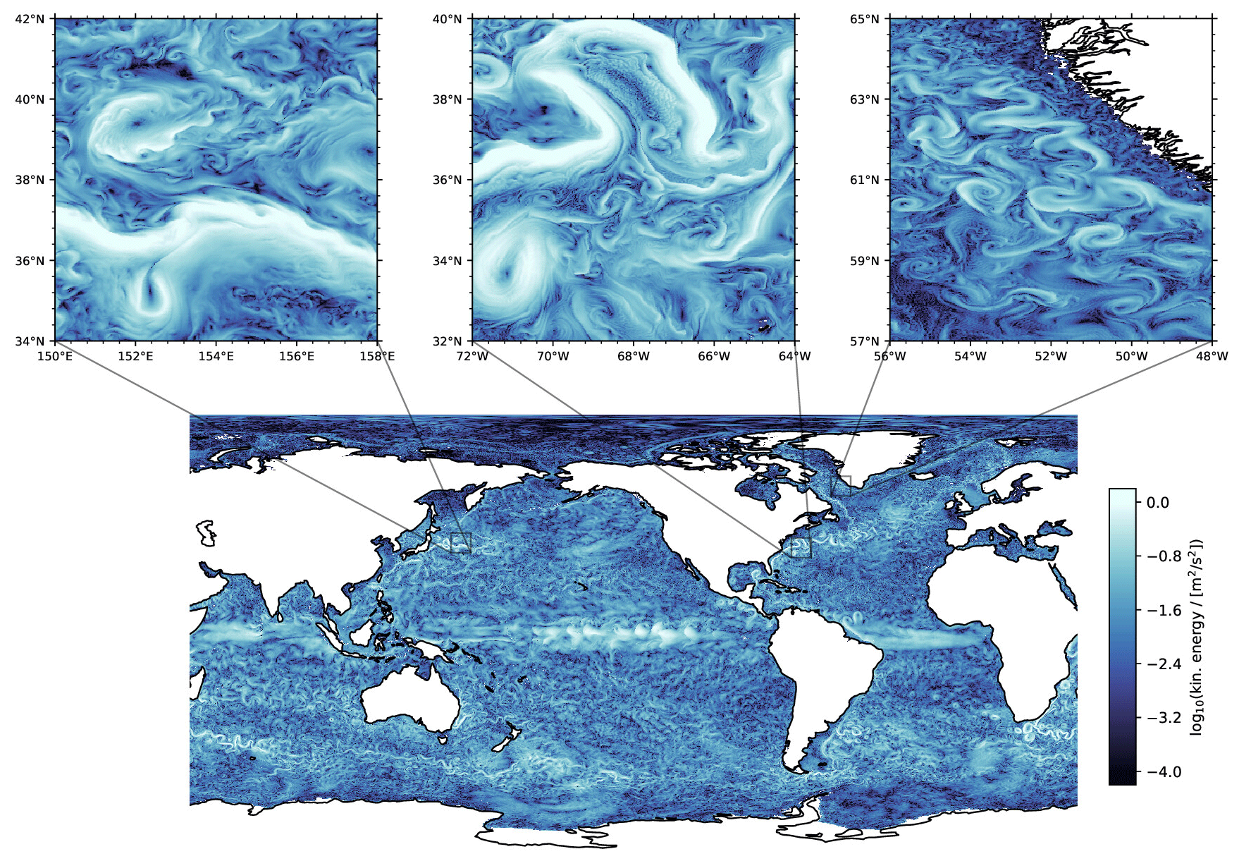
Figure 16Snapshot of kinetic energy of G_O_1.25km with three additional zooms to highlight the richness of the dynamics that can be simulated at this resolution.
One question to be answered within ICON-Sapphire is at which grid spacing we can expect submesoscale turbulence to develop. Here, we use the local Rossby number as a proxy for ageostrophic submesoscale dynamics and compare four different grid spacings by making use of the simulations G_AO_5km, G_AO_2.5km, G_O_1.25km, and G_AO_tel (Fig. 17). It becomes apparent that for grid spacings of 5 and 2.5 km, the Rossby number remains mostly smaller than 1 and only approaches 1 within the strong meanders of the Gulf Stream. In contrast, G_O_1.25km and G_AO_tel clearly show high Rossby numbers over much wider areas. In particular in G_AO_tel but also in G_O_1.25km, submesoscale eddies and fronts can be detected. Moreover, within the two simulations G_O_1.25km and G_AO_tel, submesoscale eddies and also the Gulf Stream northern wall, with narrow troughs and broad crests above which we observe reduced submesoscale activity, can be seen. The flow features are similar to what has become familiar in simulations conducted on limited-area domains (see Fig. 21 in Chassignet and Xu, 2017). Given Fig. 17, we conclude that for our ICON-Sapphire configuration in the North Atlantic during boreal winter, the critical grid spacing to allow for submesoscale dynamics is somewhere between 2.5 and 1 km. Also, we conclude that the telescope feature works as intended and can even be used coupled to an atmosphere.
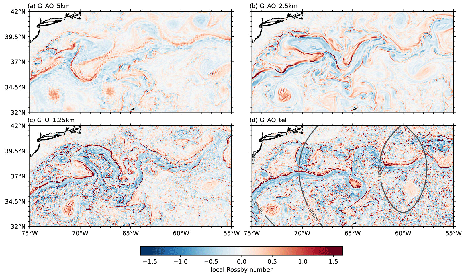
Figure 17Local Rossby number defined as relative vorticity divided by planetary vorticity over the North Atlantic in the surface layer. The Rossby number is shown for (a) G_AO_5km, (b) G_AO_2.5km, (c) G_O_1.25km, and (d) G_AO_tel. Snapshot taken after 40 d in (a)–(c) and 30 d in (d). In (d) contour lines depicting the grid spacing are also shown.
4.4 ICON-Sapphire as an ESM
ICON-Sapphire includes all the components of an ESM inherited through past modeling efforts at MPI-M. As a first step towards simulating interactively carbon at kilometer scales, we present in this section the results of a global ocean-only simulation run at 10 km (R2B8) with ocean biogeochemistry, which is one prerequisite for including an interactive carbon cycle. Phytoplankton induces radiative heating by absorbing shortwave radiation in the ocean. This in turn affects ocean physics as well as the carbon cycle and thus climate (Paulsen et al., 2018; Asselot et al., 2021). The presented simulation is referred to as G_OC_10km for a global ocean-only simulation with carbon and the suffix for the grid spacing (Table 3). It is run for 4 years from 2013 to 2016 and forced by ERA5. To initialize the model, the physical ocean fields are taken from a spun-up ocean-only 10 km simulation. The initial biogeochemical fields are interpolated from a well-spun-up 40 km run. Results from the last year of the simulation (2016) are used for model evaluation. The simulated phytoplankton concentration is converted into chlorophyll a concentration using a constant PChl ratio and compared to satellite observations from the Moderate Resolution Imaging Spectroradiometer (MODIS-Aqua) (see Fig. 18). Given the maximum optical depth that satellite sensors can ultimately perceive (Gordon and McCluney, 1975), the simulated phytoplankton concentration is averaged over the upper 30 m.
As shown by Fig. 18, G_OC_10km captures the observed spatial pattern of the yearly mean chlorophyll a concentration, with low concentrations in the subtropical gyres and high concentrations in the equatorial region, North Atlantic, North Pacific, and Southern Ocean (Fig. 18a, c). The concentrations are overestimated, but given the simplified representation of biology in HAMOCC with the use of a bulk phytoplankton and the large uncertainties in the observations (35 %), this first comparison looks generally promising. In the equatorial region, G_OC_10km overestimates the chlorophyll a concentration due to nutrient trapping, similar to previous studies (Ilyina et al., 2013). Moreover, zooming into the North Atlantic region, Fig. 18b and d indeed reveal that G_OC_10km can capture the effect of mesoscale ocean eddies on ocean productivity, as expected from observations. G_OC_10km can also reproduce the seasonal cycle in chlorophyll a concentration for the two hemispheres. In the Northern Hemisphere, the simulated seasonal cycle is in reasonable agreement with observations (not shown). It captures the spring bloom but not the autumn one. In the Southern Hemisphere, the austral summer bloom is reproduced but with an amplitude that is much too strong, with simulated concentrations around 1.75 mg m−3 in December and January versus 0.25 mg m−3 in observations. The overestimation is likely due to a lack of production in ice-covered regions in G_OC_10km, leading to a large abundance of nutrients when the ice melts.
The large-scale pattern displayed by G_OC_10km in Fig. 18a is reminiscent of the large-scale pattern displayed by the 40 km spin-up simulation. The two fields correlate with a correlation coefficient of 0.89 for the yearly mean. However, the mesoscale structures displayed by Fig. 18b are clearly absent in the spin-up simulation. Also, we can already see differences during the blooming season between the two simulations, with G_OC_10km simulating a lower chlorophyll a concentration than the spin-up simulation, in better agreement with observations. In the Northern Hemisphere, peak values are 1.5 mg m−3 in the 40 km spin-up simulation, 1.25 mg m−3 in G_OC_10km, and 0.88 mg m−3 in observations. Whether these differences are due to the representation of mesoscale eddies is too early to tell but is a further argument for being able to run ICON-Sapphire as an ESM on longer timescales.
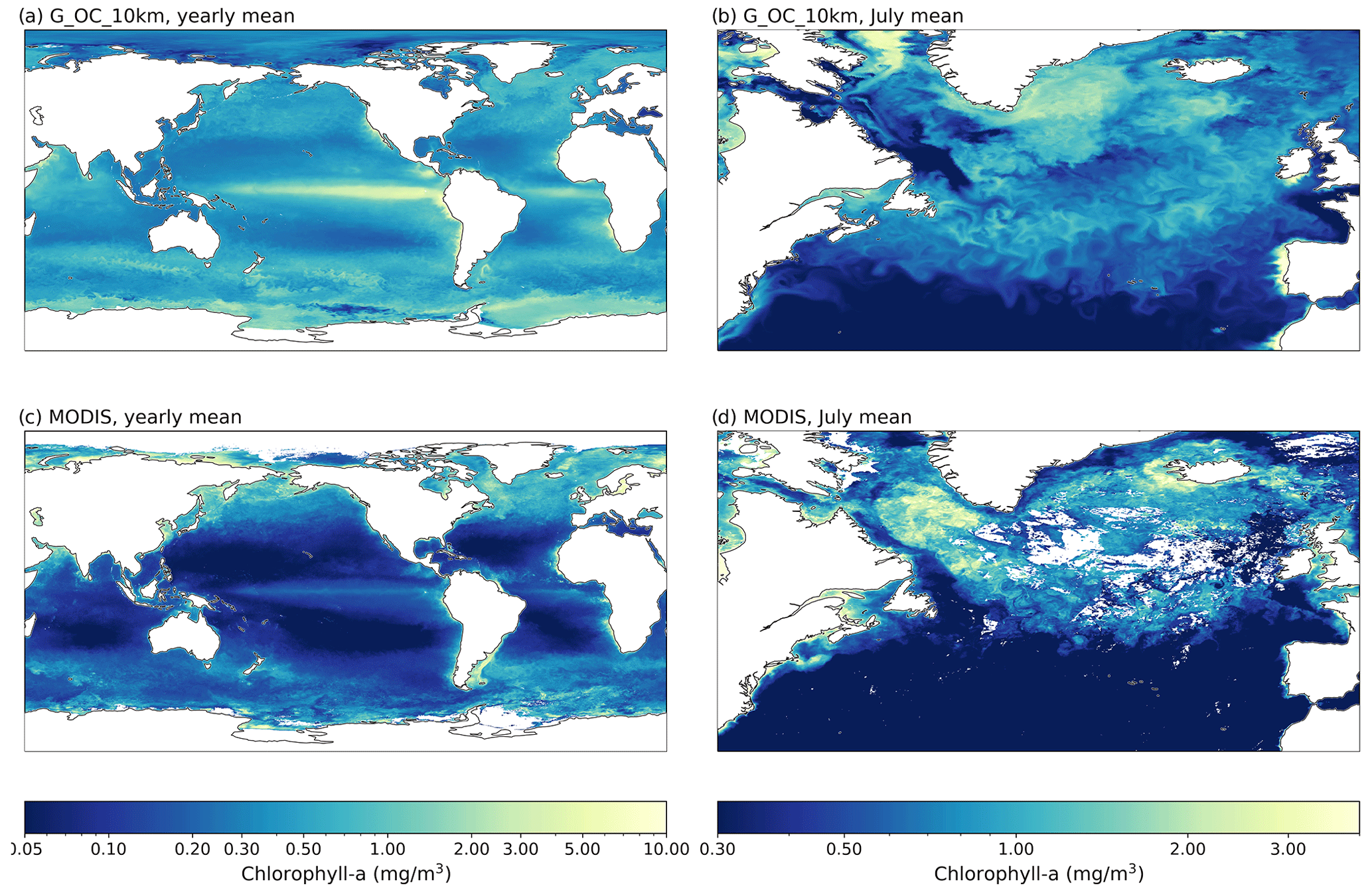
Figure 18Chlorophyll a from (a, b) G_OC_10km and (c, d) MODIS observations (grid spacing of 4 km) depicting (a, c) its global yearly mean distribution and (b, d) a zoomed-in view of the North Atlantic for July 2016.
We have presented the new ICON-Sapphire model configuration developed at the Max Planck Institute for Meteorology in cooperation with the German Climate Computing Center, a configuration designed to resolve phenomena on small spatial scales on the globe with targeted grid spacings finer than 10 km. In contrast to models currently employed at such grid spacings, ICON-Sapphire contains all components of a traditional ESM, including an interactive ocean, ocean biogeochemistry, and dynamical vegetation. We demonstrate that ICON-Sapphire can be run coupled for 1 year with a grid spacing of 5 km, for a few months with a grid spacing of 2.5 km, and even for a few days with a grid spacing of 1.25 km. In the atmosphere, hectometer grid spacings can be achieved by using the ICON capability of an inside nest and/or limited-area domain with prescribed or doubly periodic lateral boundary conditions. In the ocean, hectometer grid spacings can be achieved by using a telescope feature over specific regions, both uncoupled and coupled to a uniform atmosphere. The highest achieved grid spacing in the ocean is 1.25 km globally and down to 530 m over the North Atlantic using the telescoping feature. Results of an ocean-only simulation including ocean biogeochemistry and integrated for 4 years with a grid spacing of 10 km are also presented to demonstrate the ESM ability of ICON-Sapphire.
From the results of our 1-year global coupled simulation at 5 km with its sister simulation at 2.5 km for a few months, we find that ICON-Sapphire reproduces many features of the climate system more or less out of the box: the position and strength of the large-scale pressure systems and of the jet, the seasonal cycle in precipitation and soil moisture, salinity, the daily warming of the upper ocean in subsiding regions, the structure of the ITCZ in deep convective regions, the structure of the atmosphere above the Gulf Stream in the midlatitudes, and the coupling strength between SST, latent heat flux, and precipitation over the ocean. The main shortcomings are energy leaks, that cancel themselves out, a yearly negative radiative imbalance of 4 W m−2 at the top of the atmosphere, leading to a mean temperature that is too low, and a general overestimation of precipitation amounts except for a pronounced underestimation of precipitation at the Equator. The equatorial region also stands out with water that is too cold and too salty. Finally, there are some indications that the warming and cooling of the ocean surface do not propagate far enough into the ocean interior, indicative of ocean mixed layers that are too shallow. Through the development cycle, we also noticed a strong sensitivity of the tropical atmosphere to initial SSTs, with, for instance, small differences in initial SSTs leading to spurious formation of westerlies over the eastern tropical Atlantic accompanied by a northward propagation of the rain belt that is too weak. Some of these biases may be linked to each other but they also highlight mixing in both the ocean and the atmospheric boundary layer as a potential weak spot of kilometer-scale coupled models. Although the current TOA energy imbalance prevents long integrations of ICON-Sapphire, the present model version already allows investigating scientific questions that do not require a long integration period, such as factors controlling the seasonal migration of tropical rain belts or air–sea fluxes, for the first time in a coupled system without having to rely on numerous parameterizations.
The employed grid spacing allows resolving interactions between small and large scales across components of the Earth system, as visually demonstrated by four examples: the development of a low-pressure system over the Southern Ocean with its associated imprint on the atmosphere and the ocean, the breaking of tropical instability waves with the development of secondary SST fronts and their imprint on the surface fluxes, the breakup of the Arctic sea ice pack and the formation of leads and polynyas by a low-pressure system with its imprint on the surface fluxes, and the diurnal evolution of land–sea breezes and their forcing on convective precipitation. Furthermore, we show that ICON-Sapphire can reproduce mesoscale patterns of trade-cumulus organization in a limited-area atmosphere-only simulation using a grid spacing of 620 and 308 m and that local Rossby numbers of order 1, indicative of submesoscale eddy activity, are produced with ocean grid spacings of 1.25 km and finer. Finally, from our 10 km ocean simulation including ocean biogeochemistry, we conclude that ICON-Sapphire can capture the effect of mesoscale ocean eddies on ocean productivity, as expected from observations.
The throughput of ICON-Sapphire with a grid spacing of 5 km is 126 simulated days per day using 600 nodes on the newest machine (Levante) of DKRZ, making integrations on multi-decadal timescales possible. Multi-decadal simulations at 2.5 and 1.25 km are still out of reach on a CPU machine like Levante. The atmosphere and land components of ICON have been ported and run onto GPUs (Giorgetta et al., 2022), and a hybrid coupled ICON-Sapphire version using GPUs for the land and atmosphere and CPUs for the ocean is currently being tested on JUWELS Booster. Extrapolating from past experience, we expect that by using half of the LUMI machine, a throughput of 1 SYPD could be achieved at 2.5 km, which is a throughput generally thought to be needed for a climate simulation to be considered useful. As a next step, the ocean component of ICON-Sapphire will be ported to GPUs, as the performance of the ocean model becomes a bottleneck below a grid spacing of 5 km. Also, the atmosphere code is being simplified and refactored to better express the simplicity that arises when many of the parameterizations of traditional general circulation models (GCMs) begin to be explicitly represented. One further aim of the refactoring is to better enable scalable development to different architectures. On the physics side, the use of thin layers in the upper ocean, which is possible with the implemented new z* coordinate, the inclusion of river discharge, and a better representation of energy and ocean mixing will be in focus. An important aspect of the conducted simulations is workflow. Often data problems are data management problems; for instance, orders of magnitude improvements in data access can be achieved by intelligently structuring and indexing the data. Moreover, encoding and decoding approaches from machine learning are being developed to interpolate from sparse data, allowing for a reduction of disk space usage. Despite the remaining technical challenges, ICON-Sapphire already allows performing unique multi-decadal climate simulations, with explicit interactions between small and large scales as well as between the components of the Earth system – ocean, atmosphere, land, and cryosphere – including carbon at the forefront of exascale climate computing.
Simulations were done with the ICON branch nextgems_cycle1_dpp0066 as commit62dbfc. This source code is available here: https://doi.org/10.17617/3.1XTSR6 (Hohenegger, 2022). The ICON model is available to individuals under licenses (https://mpimet.mpg.de/en/science/modeling-with-icon/code-availability, last access: 17 January 2023). By downloading the ICON source code, the user accepts the license agreement. The observational data sets CERES-EBAF (https://doi.org/10.5067/TERRA-AQUA/CERES/EBAF_L3B.004.1, NASA/LARC/SD/ASDC, 2019), HadCRUT (https://catalogue.ceda.ac.uk/uuid/b9698c5ecf754b1d981728c37d3a9f02, Met Office Hadley Centre et al., 2020; Morice et al., 2021), GPCP (https://doi.org/10.7289/V56971M6, Adler et al., 2016), ESACCI (http://www.esa-soilmoisture-cci.org, Department of Geodesy and Geoinformation, Technical University of Vienna, 2022; Dorigo et al., 2017; Gruber et al., 2017, 2019), PHC (http://psc.apl.washington.edu/nonwp_projects/PHC/Climatology.html, Steele et al., 2001), OISST (https://doi.org/10.25921/RE9P-PT57, Huang et al., 2020), IMERG (https://doi.org/10.5067/GPM/IMERG/3B-HH/06, Huffman et al., 2019), and MODIS-aqua chlorophyll a (https://doi.org/10.5067/AQUA/MODIS/L3M/CHL/2022, NASA Goddard Space Flight Center et al., 2022) were obtained from https://www.cen.uni-hamburg.de/en/icdc/data.html (last access: 15 July 2022). ERA5 (https://doi.org/10.24381/cds.f17050d7, Hersbach et al., 2019a, https://doi.org/10.24381/cds.6860a573, Hersbach et al., 2019b) was obtained from https://cds.climate.copernicus.eu/#!/home (last access: 15 July 2022). OAFlux was obtained from https://oaflux.whoi.edu/ and is the third release of the OAFlux products (Yu et al., 2008). PATMOS was obtained from https://observations.ipsl.fr/aeris/eurec4a-data/SATELLITES/GOES-E/2km_10min/2020/ (NOAA/NESDIS and the University of Wisconsin-Madison/CIMSS, 2023). The simulation outputs from the DYAMOND intercomparison project can be obtained from https://www.esiwace.eu/services/dyamond-initiative/ (Stevens et al., 2019). Scripts employed to produce the figures can be found here: https://owncloud.gwdg.de/index.php/s/kn7GYFi3QmHmtFQ (last access: 17 January 2023).
All authors contributed to the development of the ICON-Sapphire configuration. Analysis of results was conducted by CH, JB, SB, MBeh, MBer, RB, NB, LC, FC, GD, GG, OG, HH, JJ, MK, DK, JL, TM, LP, DSP, DP, FS, HS, RShe, MS, RV, CW, and MW. The Sapphire project is led by BS and CH. The paper was written by CH with inputs, comments, and reviews from PK, LL, RR, RSch, JB, SB, MBeh, NB, FC, GD, MG, OG, TI, JJ, DK, JL, AKN, LP, DSP, DP, SR, TR, FS, HS, RShe, CCS, JSvS, RV, MW, JM, and BS.
The contact author has declared that none of the authors has any competing interests.
Publisher's note: Copernicus Publications remains neutral with regard to jurisdictional claims in published maps and institutional affiliations.
Fatemeh Chegini, Tatiana Ilyina, Ann Kirstin Naumann, and Dian Putrasahan received funding from the Deutsche Forschungsgemeinschaft (DFG, German Research Foundation) under Germany's Excellence Strategy – EXC 2037 “CLICCS – Climate, Climatic Change, and Society” – project number 390683824. George Datseris is funded by the European Horizon 2020 project CONSTRAIN, grant number 820829. Raphaela Vogel received funding from the European Research Council EUREC4A under grant agreement 694768. Swantje Bastin, Cathy Hohenegger, Johann Jungclaus, Divya Sri Praturi, and Bjorn Stevens received funding from the European Union's Horizon 2020 research and innovation program project NextGEMS under grant agreement number 101003470. Nils Brüggemann, Oliver Gutjahr, Radomyra Shevchenko, and Johann Jungclaus received funding from the Collaborative Research Centre TRR 181 “Energy Transfers in Atmosphere and Ocean” funded by the Deutsche Forschungsgemeinschaft (DFG, German Research Foundation) – project number 274762653. Florian Schütte is funded by the Bundesministerium für Bildung und Forschung as part of the NextG-Climate Science-EUREC4A-OA project. Tatiana Ilyina was supported by the European Union's Horizon 2020 research and innovation program under grant agreement 101003536 (ESM2025 – Earth System Models for the Future) and under grant agreement 820989 (COMFORT). Tatiana Ilyina and Fatemeh Chegini were supported by the European Union's Horizon 2020 research and innovation program under grant agreement 773421 – project “Nunataryuk”. Hans Segura is funded by the Hans-Ertel Centre for Weather Research under project number 4818DWDP1A. This research network of universities, research institutes, and the Deutscher Wetterdienst is funded by the Federal Ministry of Transport and Digital Infrastructure (BMVI). We acknowledge the mission scientists and associated personnel for the production of the observational data as well as the modeling teams participating in the DYAMOND intercomparison project. DYAMOND data management was provided by the German Climate Computing Center (DKRZ) and supported through the projects ESiWACE and ESiWACE2. The projects ESiWACE and ESiWACE2 have received funding from the European Union's Horizon 2020 research and innovation program under grant agreement nos. 675191 and 823988. We thank DKRZ for use of its computer facilities on which the simulations were conducted. We thank the two reviewers Roberts Malcom and Peter Caldwell for their thorough review and helpful comments that improved this paper.
This research has been supported by the Deutsche Forschungsgemeinschaft (grant nos.
390683824 and 274762653), Horizon 2020 (COMFORT (grant no. 820989), CONSTRAIN (grant no.
820829), ESiWACE (grant no 675191), ESiWACE2 (grant no 823988), ESM2025 – Earth System
Models for the Future (grant no. 101003536), EUREC4A (grant no. 694768), NextGEMS (grant no.
101003470), Nunataryuk (grant no. 773421)), the Bundesministerium für Bildung und Forschung
(NextG-Climate Science-EUREC4A-OA), and the Bundesministerium für Verkehr und
Digitale Infrastruktur (grant no. 4818DWDP1A).
The article processing charges for this open-access publication were covered by the Max Planck Society.
This paper was edited by Qiang Wang and reviewed by Malcolm Roberts and Peter Caldwell.
Adler, R., Wang, J.-J., Sapiano, M., Huffman, G., Chiu, L., Xie, P. P., Ferraro, R., Schneider, U., Becker, A., Bolvin, D., Nelkin, E., Gu, G., and NOAA CDR Program: Global Precipitation Climatology Project (GPCP) Climate Data Record (CDR), Version 2.3 (Monthly), National Centers for Environmental Information [data set], https://doi.org/10.7289/V56971M6 (last access: 15 July 2022), 2016. a
Adler, R. F., Sapiano, M. R. P., Huffman, G. J., Wang, J.-J., Gu, G., Bolvin, D., Chiu, L., Schneider, U., Becker, A., Nelkin, E., Xie, P., Ferraro, R., and Shin, D.-B.: The Global Precipitation Climatology Project (GPCP) Monthly Analysis (New Version 2.3) and a review of 2017 Global Precipitation, Atmosphere, 9, 138, https://doi.org/10.3390/atmos9040138, 2018. a
Asselot, R., Lunkeit, F., Holden, P. B., and Hense, I.: The relative importance of phytoplankton light absorption and ecosystem complexity in an Earth system model, J. Adv. Model. Earth Systems, 13, e2020MS002110, https://doi.org/10.1029/2020MS002110, 2021. a
Baldauf, M., Seifert, A., Förstner, J., Majewski, D., Raschendorfer, M., and Reinhardt, T.: Operational convective-scale numerical weather prediction with the COSMO model: Description and sensitivities, Mon. Weather Rev., 139, 3887–3905, 2011. a
Ban, N., Schmidli, J., and Schär, C.: Evaluation of the convection-resolving regional climate modeling approach in decade-long simulations, J. Geophys. Res., 119, 7889–7907, 2014. a
Becker, J. J., Sandwell, D. T., Smith, W. H. F., Braud, J., Binder, B., Depner, J., Fabre, D., Factor, J., Ingalls, S., Kim, S.-H., Ladner, R., Marks, K., Nelson, S., Pharaoh, A., Trimmer, R., Von Rosenberg, J., Wallace, G., and Weatherall, P.: Global bathymetry and elevation data at 30 arc seconds resolution: SRTM30PLUS, Mar. Geod., 32, 355–371, 2009. a
Bretherton, C. S. and Khairoutdinov, M. F.: Convective self-aggregation feedbacks in near-global cloud-resolving simulations of an aquaplanet, J. Adv. Model. Earth Sy., 7, 1765–1787, 2015. a
Bryan, G. H., Wyngaard, J. C., and Fritsch, J. M.: Resolution requirements for simulations of deep moist convection, Mon. Weather Rev., 131, 2394–2416, 2003. a
Capet, X., McWilliams, J., Molemaker, M., and Shchepetkin, A. F.: Mesoscale to submesoscale transition in the California current system. Part I: flow structure, eddy flux, and observational tests, J. Phys. Oceanogr., 38, 29–43, 2008. a
Chang, P., Zhang, S., Danabasoglu, G., Yeager, S. G., Fu, H., Wang, H., Castruccio, F. S., Chen, Y., Edwards, J., Fu, D., Jia, Y., Laurindo, L. C., Lui, X., Rosenbloom, N., Small, R. J., Xu, G., Zeng, Y., Zhang, Q., Bacmeister, J., Bailey, D. A., Duan, X., DuVivier, A. K., Li, D., Li, Y., Neale, R., Stössel, A., Wang, L., Zhuang, Y., Baker, A., Bates, S., Dennis, J., Diao, X., Gan, B., Gopal, A., Jia, D., Jing, Z., Ma, X., Saravanan, R., Strand, W. G., Tao, J., Yang, H., Wang, X., Wei, Z., and Wu, L.: An unprecedented set of high-resolution Earth system simulations for understanding multiscale interactions in climate variability and change, J. Adv. Model. Earth Sy., 12, e2020MS002298, https://doi.org/10.1029/2020MS002298, 2020. a
Chassignet, E. P. and Xu, X.: Impact of horizontal resolution ( to ) on Gulf Stream separation, penetration and variability, J. Phys. Oceanogr., 47, 1999–2021, https://doi.org/10.1175/JPO-D-17-0031.1, 2017. a, b
Chassignet, E. P. and Xu, X.: On the importance of high-resolution in large-scale ocean models, Adv. Atm. Sci., 38, 1621–1634, 2021. a
Chen, D., Rojas, M., Samset, B. H., Cobb, K., Diongue Niang, A., Edwards, P., Emori, S., Faria, S., Hawkins, E., Hope, P., Huybrechts, P., Meinshausen, M., Mustafa, S. K., Plattner, G.-K., and Tréguie, A.-M.: Framing, Context, and Methods, Climate Change 2021: The Physical Science Basis. Contribution of Working Group I to the Sixth Assessment Report of the Intergovernmental Panel on Climate Change, edited by: Masson-Delmotte, V., Zhai, P., Pirani, A., Connors, S. L., Péan, C., Berger, S., Caud, N., Chen, Y., Goldfarb, L., Gomis, M. I., Huang, M., Leitzell, K., Lonnoy, E., Matthews, J. B. R., Maycock, T. K., Waterfield, T., Yelekçi, O., Yu, R., and Zhou, B., Cambridge University Press, Cambridge, United Kingdom and New York, NY, USA, 147–286, https://doi.org/10.1017/9781009157896.003, 2021. a
Danilov, S., Wang, Q., Timmermann, R., Iakovlev, N., Sidorenko, D., Kimmritz, M., Jung, T., and Schröter, J.: Finite-Element Sea Ice Model (FESIM), version 2, Geosci. Model Dev., 8, 1747–1761, https://doi.org/10.5194/gmd-8-1747-2015, 2015. a
Department of Geodesy and Geoinformation, Technical University of Vienna: ESA CCI Surface Soil Moisture COMBINED active+passive Product, Technical University of Vienna [data set], http://www.esa-soilmoisture-cci.org, last access: 15 July 2022. a
de Vrese, P., Stacke, T., Kleinen, T., and Brovkin, V.: Diverging responses of high-latitude CO2 and CH4 emissions in idealized climate change scenarios, The Cryosphere, 15, 1097–1130, https://doi.org/10.5194/tc-15-1097-2021, 2021. a
Dipankar, A., Stevens, B., Heinze, R., Moseley, C., Zängl, G., Giorgetta, M., and Brdar, S.: Large eddy simulation using the general circulation model ICON, J. Adv. Model. Earth Sy., 7, 963–986, 2015. a, b
Donohue, K. A., Tracey, K. L., Watts, D. R. andChidichimo, M. P., and Chereskin, T. K.: Mean Antarctic Circumpoloar current transport measured in Drake Passage, Geophys. Res. Lett., 9, 3231–3296, 2016. a
Dorigo, W. A., Wagner, W., Albergel, C., Albrecht, F., Balsamo, G., Brocca, L., Chung, D., Ertl, M., Forkel, M., Gruber, A., Haas, E., Hamer, D. P. Hirschi, M., Ikonen, J., De Jeu, R. Kidd, R. Lahoz, W., Liu, Y.Y., Miralles, D., and Lecomte, P.: ESA CCI Soil Moisture for improved Earth system understanding: State-of-the art and future directions. Remote Sensing of Environment, 203, 185–215, https://doi.org/10.1016/j.rse.2017.07.001, 2017. a, b
Ekici, A., Beer, C., Hagemann, S., Boike, J., Langer, M., and Hauck, C.: Simulating high-latitude permafrost regions by the JSBACH terrestrial ecosystem model, Geosci. Model Dev., 7, 631–647, https://doi.org/10.5194/gmd-7-631-2014, 2014. a
Fiedler, S., Crueger, T., D'Agostino, R., Peters, K., Becker, T., Leutwyler, D., Paccini, L., Burdanowitz, J., Buehler, S. A., Cortes, A. U., Dauhut, T., Dommenget, D., Fraedrich, K., Jungandreas, L., Maher, N., Naumann, A. K., Rugenstein, M., Sakradzija, M., Schmidt, H., Sielmann, F., Stephan, C., Timmreck, C., Zhu, X., and Stevens, B.: Simulated tropical precipitation assessed across three phases of the Coupled Model Intercomparison Project (CMIP), Mon. Weather Rev., 148, 3653–3680, 2020. a
Flato, G. M.: Earth system models: an overview, WIREs Clim. Change, 2, 783–800, https://doi.org/10.1002/wcc.148, 2011. a
Flexas, M. M., Thompson, A. F., Torres, H. S., Klein, P., Farrar, J. T., Zhang, H., and Menemenlis, D.: Global estimates of the energy transfer from the wind to the ocean, with emphasis on near-inertial oscillations, J. Geophys. Res.-Oceans, 124, 5723–5746, https://doi.org/10.1029/2018JC014453, 2019. a, b
Fox-Kemper, B. and Menemenlis, D.: Can large eddy simulation techniques improve mesoscale rich ocean models?, Ocean Modelling in an Eddying Regime, 177, 319–337, https://doi.org/10.1029/177GM19, 2008. a
Fox-Kemper, B., Danabasoglu, G., Ferrari, R., Griffies, S. M., Hallberg, R. W., Holland, M. M., Altrud, M. E., Peacock, S., and Samuels, B. L.: Parameterization of mixed layer eddies. III: Implementation and impact in global ocean climate simulations, Ocean Model., 39, 61–78, 2011. a
Frassoni, A., Castilho, D., Rixen, M., Ramirez, E., de Mattos, J. G. Z., Kubota, P., Calheiros, A. J. P., Reed, K. A., Assuncao, M., da Silva Dias, F., da Silva Dias, P. L., de Campos Velho, H. F., de Roode, S. R., Doblas-Reyes, F., Eiras, D., Ek, M., Figueroa, S. N., Forbes, R., Freitas, S. R., Grell, G. A., Herdis, D. L., Lauritzen, P. H., Machado, L. A. T., Manzi, A. O., Martins, G., Oliveria, G. S., Rosario, N. E., Sales, D. C., Wedi, N., and Yamada, B.: Building the next generation of climate modelers: Scale-aware physics parameterization and the ”Grey Zone” challenge, B. Am. Meteorol. Soc., 99, ES185–ES189, https://doi.org/10.1175/BAMS-D-18-0145.1, 2018. a
Fuhrer, O., Chadha, T., Hoefler, T., Kwasniewski, G., Lapillonne, X., Leutwyler, D., Lüthi, D., Osuna, C., Schär, C., Schulthess, T. C., and Vogt, H.: Near-global climate simulation at 1 km resolution: establishing a performance baseline on 4888 GPUs with COSMO 5.0, Geosci. Model Dev., 11, 1665–1681, https://doi.org/10.5194/gmd-11-1665-2018, 2018. a
GARP (Ed.): The physical basis of climate and climate modelling, vol. 16 of GARP publications series, World Meteorological Organization, International Council of Scientific Unions, Geneva, Switzerland, 1975. a
Gaspar, P., Gregoris, Y., and Lefebre, J.-M.: A simple eddy kinetic energy model for simulations of the oceanic vertical mixing: Tests at station Papa and long-term upper ocean study site, J. Geophys. Res.-Oceans, 95, 16179–16193, https://doi.org/10.1029/JC095iC09p16179, 1990. a
Gassmann, A.: A global hexagonal C-grid non-hydrostatic dynamical core (ICON-IAP) designed for energetic consistency, Q. J. Roy. Meteor. Soc., 139, 152–175, 2013. a
Gassmann, A. and Herzog, H. J.: Towards a consistent numerical compressible non-hydrostatic model using generalized Hamiltonian tools, Q. J. Roy. Meteor. Soc., 134, 1597–1613, 2008. a
Giorgetta, M. A., Brokopf, R., Crueger, T., Esch, M., Fiedler, S., Helmert, J., Hohenegger, C., Kornblueh, L., Kohler, M., Manzini, E., Mauritsen, T., Nam, C., Raddatz, T., Rast, S., Reinert, D., Sakradzija, M., Schmidt, H., Schneck, R., Schnur, R., Silvers, L., Wan, H., Zangl, G., and Stevens, B.: ICON-A, the atmosphere component of the ICON Earth system model: I. Model description, J. Adv. Model. Earth Sy., 10, 1613–1637, https://doi.org/10.1029/2017ms001242, 2018. a, b
Giorgetta, M. A., Sawyer, W., Lapillonne, X., Adamidis, P., Alexeev, D., Clément, V., Dietlicher, R., Engels, J. F., Esch, M., Franke, H., Frauen, C., Hannah, W. M., Hillman, B. R., Kornblueh, L., Marti, P., Norman, M. R., Pincus, R., Rast, S., Reinert, D., Schnur, R., Schulzweida, U., and Stevens, B.: The ICON-A model for direct QBO simulations on GPUs (version icon-cscs:baf28a514), Geosci. Model Dev., 15, 6985–7016, https://doi.org/10.5194/gmd-15-6985-2022, 2022. a, b, c
Gordon, H. R. and McCluney, W.: Estimation of the depth of sunlight penetration in the sea for remote sensing, Appl. Optics, 14, 413–416, 1975. a
Grell, G. A., Schade, L., Knoche, R., Pfeiffer, A., and Egger, J.: Nonhydrostatic climate simulations of precipitation over complex terrain, J. Geophys. Res., 105, 29595–29608, 2000. a
Griffies, S. M., Winton, M., Anderson, W. G., Benson, R., Delworth, T. L., Dufour, C. O., Dunne, J. P., Goddard, P., Morrison, A. K., Rosati, A., Wittenberg, A. T., Yin, J., and Zhang, R.: Impacts on ocean heat from transient mesoscale eddies in a hierarchy of climate models, J. Climate, 28, 952–977, https://doi.org/10.1175/JCLI-D-14-00353.1, 2015. a
Griffies, S. M., Danabasoglu, G., Durack, P. J., Adcroft, A. J., Balaji, V., Böning, C. W., Chassignet, E. P., Curchitser, E., Deshayes, J., Drange, H., Fox-Kemper, B., Gleckler, P. J., Gregory, J. M., Haak, H., Hallberg, R. W., Heimbach, P., Hewitt, H. T., Holland, D. M., Ilyina, T., Jungclaus, J. H., Komuro, Y., Krasting, J. P., Large, W. G., Marsland, S. J., Masina, S., McDougall, T. J., Nurser, A. J. G., Orr, J. C., Pirani, A., Qiao, F., Stouffer, R. J., Taylor, K. E., Treguier, A. M., Tsujino, H., Uotila, P., Valdivieso, M., Wang, Q., Winton, M., and Yeager, S. G.: OMIP contribution to CMIP6: experimental and diagnostic protocol for the physical component of the Ocean Model Intercomparison Project, Geosci. Model Dev., 9, 3231–3296, https://doi.org/10.5194/gmd-9-3231-2016, 2016. a
Gruber, A., Dorigo, W. A., Crow, W., and Wagner, W.: Triple Collocation- Based Merging of Satellite Soil Moisture Retrievals, IEEE T. Geosci. Remote, 55, 6780–6792, https://doi.org/10.1109/TGRS.2017.2734070, 2017. a
Gruber, A., Scanlon, T., van der Schalie, R., Wagner, W., and Dorigo, W.: Evolution of the ESA CCI Soil Moisture climate data records and their underlying merging methodology, Earth Syst. Sci. Data, 11, 717–739, https://doi.org/10.5194/essd-11-717-2019, 2019. a
Gula, J., Molemaker, M. J., and McWilliams, J. C.: Submesoscale dynamics of a Gulf Stream frontal eddy in the South Atlantic Bight, J. Phys. Oceanogr., 46, 305–325, https://doi.org/10.1175/JPO-D-14-0258.1, 2016. a
Gutjahr, O., Jungclaus, J. H., Brüggemann, N., Haak, H., and Marotzke, J.: Air-sea interactions and water mass transformation during a katabatic storm in the Irminger Sea, J. Geophys. Res.-Oceans, 127, e2021JC018075, https://doi.org/10.1029/2021JC018075, 2022. a
Haarsma, R. J., Roberts, M. J., Vidale, P. L., Senior, C. A., Bellucci, A., Bao, Q., Chang, P., Corti, S., Fučkar, N. S., Guemas, V., von Hardenberg, J., Hazeleger, W., Kodama, C., Koenigk, T., Leung, L. R., Lu, J., Luo, J.-J., Mao, J., Mizielinski, M. S., Mizuta, R., Nobre, P., Satoh, M., Scoccimarro, E., Semmler, T., Small, J., and von Storch, J.-S.: High Resolution Model Intercomparison Project (HighResMIP v1.0) for CMIP6, Geosci. Model Dev., 9, 4185–4208, https://doi.org/10.5194/gmd-9-4185-2016, 2016. a
Hagemann, S.: An Improved land surface parameter dataset for global and regional climate models, Tech. Rep. 336, Max Planck Institute for Meteorology, https://doi.org/10.17617/2.2344576, 2002. a
Hagemann, S. and Dümenil, L.: A parameterization of the lateral waterflow for the globale scale, Clim. Dynam., 14, 17–31, 1997. a
Hagemann, S. and Stacke, T.: Impact of the soil hydrology scheme on simulated soil moisture memory, Clim. Dynam., 44, 1731–1750, https://doi.org/10.1007/s00382-014-2221-6, 2015. a, b
Hanke, M., Redler, R., Holfeld, T., and Yastremsky, M.: YAC 1.2.0: new aspects for coupling software in Earth system modelling, Geosci. Model Dev., 9, 2755–2769, https://doi.org/10.5194/gmd-9-2755-2016, 2016. a
Hersbach, H., Bell, B., Berrisford, P., Biavati, G., Horányi, A., Muñoz Sabater, J., Nicolas, J., Peubey, C., Radu, R., Rozum, I., Schepers, D., Simmons, A., Soci, C., Dee, D., and Thépaut, J.-N.: ERA5 monthly averaged data on single levels from 1979 to present, Copernicus Climate Change Service (C3S) Climate Data Store (CDS) [data set], https://doi.org/10.24381/cds.f17050d7 (last access: 15 July 2022), 2019a. a
Hersbach, H., Bell, B., Berrisford, P., Biavati, G., Horányi, A., Muñoz Sabater, J., Nicolas, J., Peubey, C., Radu, R., Rozum, I., Schepers, D., Simmons, A., Soci, C., Dee and D., and Thépaut, J.-N.: ERA5 monthly averaged data on pressure levels from 1979 to present, Copernicus Climate Change Service (C3S) Climate Data Store (CDS) [data set], https://doi.org/10.24381/cds.6860a573 (last access: 15 July 2022), 2019b. a
Hersbach, H., Bell, B., Berrisford, P., Hirahara, S., Horanyi, A., Munoz-Sabater, J., Nicolas, J., Peubey, C., Radu, R., Schepers, D., Simmons, A., Soci, C., Abdalla, S., Abellan, X., Balsamo, G., Bechtold, P., Biavati, G., Bidlot, J., Bonavita, M., De Chiara, G., Dahlgren, P., Dee, D., Diamantakis, M., Dragani, R., Flemming, J., Forbes, R., Fuentes, M., Geer, A., Haimberger, L. Healy, S., Hogan, R. J., Holm, E., Janiskova, M., Keeley, S., Laloyaux, P., Lopez, P., Lupu, C., Radnoti, G., de Rosnay, P., Rozum, I., Vamborg, F., Villaume, S., and Thépaut, J.-N.: The ERA5 global analysis, Q. J. Roy. Meteor. Soc., 146, 1999–2049, 2020. a
Hewitt, H., Bell, M. J., Chassignet, E. P., Czaja, A., Ferreira, D., Griffies, S. M., Hyder, P., McClean, J. L., New, A. L., and Roberts, M. J.: Will high-resolution global ocean models benefit coupled predictions on short-range to climate timescales?, Ocean Model., 120, 120–136, 2017. a, b
Hewitt, H. T., Roberts, M. J., Hyder, P., Graham, T., Rae, J., Belcher, S. E., Bourdallé-Badie, R., Copsey, D., Coward, A., Guiavarch, C., Harris, C., Hill, R., Hirschi, J. J.-M., Madec, G., Mizielinski, M. S., Neininger, E., New, A. L., Rioual, J.-C., Sinha, B., Storkey, D., Shelly, A., Thorpe, L., and Wood, R. A.: The impact of resolving the Rossby radius at mid-latitudes in the ocean: results from a high-resolution version of the Met Office GC2 coupled model, Geosci. Model Dev., 9, 3655–3670, https://doi.org/10.5194/gmd-9-3655-2016, 2016. a
Hewitt, H. T., Roberts, M., Mathiot, P., and Coauthors.: Resolving and parameterising the ocean mesoscale in Earth system models, Current Climate Change Reports, 6, 137–152, 2020. a
Hohenegger, C.: Code for “ICON-Sapphire: simulating the components of the Earth System and their interactions at kilometer and subkilometer scales”, V1, Edmond [code], https://doi.org/10.17617/3.1XTSR6, 2022. a
Hohenegger, C. and Klocke, D.: Stürmische Zeiten für die Klimaforschung, Phys. Unserer Zeit, 228, 228–235, https://doi.org/10.1002/piuz.202001580, 2020. a
Hohenegger, C., Brockhaus, P., and Schär, C.: Towards climate simulations at cloud-resolving scales, Meteorol. Z., 17, 383–394, 2008. a
Hohenegger, C., Brockhaus, P., Bretherton, C. S., and Schär, C.: The soil moisture-precipitation feedback in simulations with explicit and parameterized convection, J. Climate, 22, 5003–5020, https://doi.org/10.1175/2009JCLI2604.1, 2009. a
Hohenegger, C., Kornblueh, L., Klocke, D., Becker, T., Cioni, G., Engels, J. F., Schulzweida, U., and Stevens, B.: Climate statistics in global simulations of the atmosphere, from 80 to 2.5 km grid spacing, J. Meteorol. Soc. Japan, 98, 73–91, https://doi.org/10.2151/jmsj.2020-005, 2020. a, b, c
Huang, B., Liu, C., Banzon, V. F., Freeman, E., Graham, G., Hankins, B., Smith, T. M., and Zhang, H.-M.: NOAA 0.25-degree Daily Optimum Interpolation Sea Surface Temperature (OISST), Version 2.1, NOAA National Centers for Environmental Information [data set], https://doi.org/10.25921/RE9P-PT57 (last access: 2 August 2022), 2020. a
Huffman, G. J., Stocker, E. F., Bolvin, D. T., Nelkin, E. J., and Tan, J.: GPM IMERG Final Precipitation L3 Half Hourly 0.1 degree × 0.1 degree V06, Greenbelt, MD, Goddard Earth Sciences Data and Information Services Center (GES DISC) [data set], https://doi.org/10.5067/GPM/IMERG/3B-HH/06 (last access: 26 February 2022), 2019. a
Ilyina, T., Six, K. D., Segschneider, J., Maier-Reimer, E., Li, H., and Núñez-Riboni, I.: Global ocean biogeochemistry model HAMOCC: Model architecture and performance as component of the MPI-Earth system model in different CMIP5 experimental realizations, J. Adv. Model. Earth Sy., 5, 287–315, 2013. a, b
Jacobs, G. A., Huntley, H. S., Kirwan, A. D., Lipphardt, B. L., Campbell, T., Smith, T., Edwards, K., and Bartels, B.: Ocean processes underlying surface clustering, J. Geophys. Res., 121, 180–197, 2016. a
Jochum, M., Murtugudde, R., Ferrari, R., and Malanotte-Rizzoli, P.: The impact of horizontal resolution on the tropical heat budget in an Atlantic Ocean Model, J. Climate, 18, 841–851, 2005. a
Jungclaus, J. H., Lorenz, S. J., Schmidt, H., Brovkin, V., Brüggemann,N., Chegini, F., Crüger, T., De-Vrese, P., Gayler, V., Giorgetta, M. A., Gutjahr, O., Haak, H., Hagemann, S., Hanke, M., Ilyina, T., Korn, P., Kröger, J., Linardakis, L., Mehlmann, C., Mikolajewicz, Müller, W. A., Nabel, J. E. M. S., Notz, D., Pohlmann, H., Putrasahan, D. A., Raddatz, T., Ramme, L., Redler, R., Reick, C. H., Riddick, T., Sam, T., Schneck, R., Schnur, R., Schupfner, M., von Storch, J.-S., Wachsmann, F., Wieners, K.-H., Ziemen, F., Stevens, B., Marotzke, J., and Claussen, M.: The ICON Earth System Model Version 1.0, J. Adv. Model. Earth Sy., 14, e2021MS002813, https://doi.org/10.1029/2021MS002813, 2022. a, b
Kalnay, E., Kanamitsu, M., Kistler, R., Collins, W., Deaven, D., Gandin, L., Iredell, M., Saha, S., White, G., Woollen, J., Zhu, Y., Chelliah, M., Ebisuzaki, W., Higgins, W., Janowiak, J., Mo, K. C., Ropelewski, C., Wang, J., Leetmaa, A., Reynolds, R. Jenne, R., and Joesph, D.: The NCEP/NCAR 40-year reanalysis project, B. Am. Meteorol. Soc., 77, 437–472, 1996. a
Keelye, S. P. E., Sutton, R. T., and Shaffrey, L. C.: The impact of North Atlantic sea surface temperature errors on the simulation of North Atlantic European region climate, Q. J. Roy. Meteor. Soc., 138, 1774–1783, 2012. a
Kinne, S.: Aerosol radiative effects with MACv2, Atmos. Chem. Phys., 19, 10919–10959, https://doi.org/10.5194/acp-19-10919-2019, 2019. a
Klemp, J. and Wilhelmson, R.: Simulation of three-dimensional convective storm dynamics, J. Atmos. Sci., 35, 1070–1096, 1978. a
Klemp, J. B., Dudhia, J., and Hassiotis, A. D.: An upper gravity-wave absorbing layer for NWP applications, Mon. Weather Rev., 136, 3987–4004, 2008. a
Konow, H., Ewald, F., George, G., Jacob, M., Klingebiel, M., Kölling, T., Luebke, A. E., Mieslinger, T., Pörtge, V., Radtke, J., Schäfer, M., Schulz, H., Vogel, R., Wirth, M., Bony, S., Crewell, S., Ehrlich, A., Forster, L., Giez, A., Gödde, F., Groß, S., Gutleben, M., Hagen, M., Hirsch, L., Jansen, F., Lang, T., Mayer, B., Mech, M., Prange, M., Schnitt, S., Vial, J., Walbröl, A., Wendisch, M., Wolf, K., Zinner, T., Zöger, M., Ament, F., and Stevens, B.: EUREC4A's HALO, Earth Sy. Sci. Data, 13, 5545–5563, https://doi.org/10.5194/essd-13-5545-2021, 2021. a
Korn, P.: A structure-preserving discretization of ocean parametrizations on unstructured grids, Ocean Model., 132, 73–90, 2018. a, b
Korn, P., Brüggemann, N., Jungclaus, J. H., Lorenz, S. J., Gutjahr, O., Haak, H., Linardakis, L., Mehlmann, C., Mikolajewicz, U., Notz, D., Putrasahan, D. A., Singh, V., von Storch, J.-S., Zhu, X., and Marotzke, J.: ICON-O: the ocean component of the ICON Earth System Model – Global simulation characteristics and local telescoping capability, J. Adv. Model. Earth Sy., 14, e2021MS002952, https://doi.org/10.1029/2021MS002952, 2022. a, b, c
Langhans, W., Schmidli, J., and Schär, C.: Bulk convergence of cloud-resolving simulations of moist convection over complex terrain, J. Atmos. Sci., 69, 2207–2228, 2012. a
Lee, J., Hohenegger, C., Chlond, A., and Schnur, R.: The climatic role of interactive leaf phenology in the vegetation-atmosphere system of radiative-convective equilibrium storm-resolving simulations, Tellus, 74, 164–175, 2022a. a, b, c
Lee, Y.-Y., Marotzke, J., Bala, G., Cao, L., Corti, S., Dunne, J. P. ., Engelbrecht, F., Fischer, E., Fyfe, E., Jones, C., Maycock, A., Mutemi, J., Ndiaye, O., Panickal, S., and Zhou, T.: Future global climate: scenario-based projections and near-term information, in: Climate Change 2021: The Physical Science Basis. Contribution of Working Group I to the Sixth Assessment Report of the Intergovernmental panel on Climate Change, edited by Masson-Delmotte, V., Zhai, P., Pirani, A., Connors, S. L., Pean, C., Berger, S., Caud, N., Chen, Y., Goldfarb, L., Gomis, I., Huang, M., Leitzell, K., Lonnoy, E., Matthews, J. B. R., Maycock, T. K., Waterfield, T., Yelekci, O., Yu, R., and Zhou, B., Cambridge University Press, Cambridge, United Kingdom and New York, NY, USA, 553–672, https://doi.org/10.1017/9781009157896.006, 2022b. a
Leuenberger, D., Koller, M., Fuhrer, O., and Schär, C.: A generalization of the SLEVE vertical coordinate, Mon. Weather Rev., 138, 3683–3689, 2010. a
Leutwyler, D., Imamovic, A., and Schär, C.: The continental-scale soil moisture-precipitation feedback in Europe with parameterized and explicit convection, J. Climate, 34, 5303–5320, https://doi.org/10.1175/JCLI-D-20-0415.1, 2021. a
Lilly, D. K.: On the numerical simulation of buyoant convection, Tellus, 2, 148–172, 1962. a
Liu, C., Ikeda, K., Rasmussen, R., Marlage, M., Newman, A. J., Prein, A. F., Chen, F., Chen, L., Clark, M., Dai, A., Dudhia, J., T., E., Gochis, D., Gutmann, E., Kurkute, S., Li, Y., Thompson, G., and Yates, D.: Continental-scale convection-permitting modeling of the current and future climate of North America, Clim. Dynam., 49, 71–95, 2017. a
Liu, X. and Schumaker, L. L.: Hybrid Bézier patches on sphere-like surfaces, J. Comput. Appl. Math., 73, 157–172, https://doi.org/10.1016/0377-0427(96)00041-6, 1996. a
Loeb, N. G., Doelling, D. R., Wang, H., Su, W., Nguyen, C., Corbett, J. G., Liang, L., Mitrescu, C., and Rose, F. G.: Clouds and the Earth's Radiant Energy System (CERES) Energy Balanced and Filled (EBAF) Top-of-Atmosphere (TOA) Edition-4.0 Data Product, J. Climate, 31, 895–918, https://doi.org//10.1175/JCLI-D-17-0208.1, 2018. a
Louis, J.-F.: A parametric model of vertical eddy fluxes in the atmosphere, Bound.-Lay. Meteorol., 17, 187–202, 1979. a
Maerz, J., Six, K. D., Stemmler, I., Ahmerkamp, S., and Ilyina, T.: Microstructure and composition of marine aggregates as co-determinants for vertical particulate organic carbon transfer in the global ocean, Biogeosciences, 17, 1765–1803, https://doi.org/10.5194/bg-17-1765-2020, 2020. a
Manabe, S., Smagorinsky, J., and Strickler, R. F.: Simulated climatology of a general circulation model with a hydrologic cycle, Mon. Weather Rev., 93, 769–798, 1965. a
Mauritsen, T., Stevens, B., Roeckner, E., Crueger, T., Esch, M., Giorgetta, M., Haak, H., Jungclaus, J., Klocke, D., Matei, D., Mikolajewicz, U., Notz, D., Pincus, R., Schmidt, H., and Tomassini, L.: Tuning the climate of a global model, J. Adv. Model. Earth Sy., 4, M00A01, https://doi.org/10.1029/2012MS000154, 2012. a
Mauritsen, T., Bader, J., Becker, T., Behrens, J., Bittner, M., Brokopf, R., Brovkin, V., Claussen, M., Crueger, T., Esch, M., Fast, I., Fiedler, S., Flaeschner, D., Gayler, V., Giorgetta, M., Goll, D. S., Haak, H., Hagemann, S., Hedemann, C., Hohenegger, C., Ilyina, T., Jahns, T., Jimenez-de-la Cuesta, D., Jungclaus, J., Kleinen, T., Kloster, S., Kracher, D., Kinne, S., Kleberg, D., Lasslop, G., Kornblueh, L., Marotzke, J., Matei, D., Meraner, K., Mikolajewicz, U., Modali, K., Mobis, B., Muller, W. A., Nabel, J. E. M. S., Nam, C. C. W., Notz, D., Nyawira, S. S., Paulsen, H., Peters, K., Pincus, R., Pohlmann, H., Pongratz, J., Popp, M., Raddatz, T. J., Rast, S., Redler, R., Reick, C. H., Rohrschneider, T., Schemann, V., Schmidt, H., Schnur, R., Schulzweida, U., Six, K. D., Stein, L., Stemmler, I., Stevens, B., von Storch, J.-S., Tian, F. X., Voigt, A., Vrese, P., Wieners, K. H., Wilkenskjeld, S., Winkler, A., and Roeckner, E.: Developments in the MPI-M Earth System Model version 1.2 (MPI-ESM1.2) and its response to increasing CO2, J. Adv. Model. Earth Sy., 11, 998–1038, https://doi.org/10.1029/2018ms001400, 2019. a
Mauritsen, T., Redler, R., Esch, M., Stevens, B., Hohenegger, C., Klocke, D., Brokopf, R., Haak, H., Linardakis, L., Röber, N., and Schnur, R.: Early development and tuning of a global coupled cloud resolving model, and its fast response to increasing CO2, Tellus A, 74, 346–363, https://doi.org/10.16993/tellusa.54, 2022. a
Mehlmann, C. and Korn, P.: Sea-ice dynamics on triangular grids, J. Comp. Phys., 428, 110086, https://doi.org/10.1016/j.jcp.2020.110086, 2021. a
Mehlmann, C., Danilov, S., Losch, M., Lemieux, J. F., Hutter, N., Richter, T., Blain, P., Hunke, E. C., and Korn, P.: Simulating linear kinematic features in viscous-plastic sea ice models on quadrilateral and triangular grids, J. Adv. Model. Earth Sy., 13, e2021MS002523, https://doi.org/10.1029/2021MS002523, 2021. a
Meinshausen, M., Vogel, E., Nauels, A., Lorbacher, K., Meinshausen, N., Etheridge, D. M., Fraser, P. J., Montzka, S. A., Rayner, P. J., Trudinger, C. M., Krummel, P. B., Beyerle, U., Canadell, J. G., Daniel, J. S., Enting, I. G., Law, R. M., Lunder, C. R., O'Doherty, S., Prinn, R. G., Reimann, S., Rubino, M., Velders, G. J. M., Vollmer, M. K., Wang, R. H. J., and Weiss, R.: Historical greenhouse gas concentrations for climate modelling (CMIP6), Geosci. Model Dev., 10, 2057–2116, https://doi.org/10.5194/gmd-10-2057-2017, 2017. a
Mellado, J. P.: Cloud-top entrainment in stratocumulus clouds, Annu. Rev. Fluid Mech., 49, 145–169, 2017. a
Met Office Hadley Centre, University of East Anglia Climatic Research Unit, Morice, C. P., Kennedy, J. J., Rayner, N. A., Winn, J. P., Hogan, E., Killick, R. E., Dunn, R. J. H., Osborn, T., Jones, P. D., and Simpson, I.: HadCRUT.5.0.0.0: Ensemble near-surface temperature anomaly grids and time series, Centre for Environmental Data Analysis [data set], https://catalogue.ceda.ac.uk/uuid/b9698c5ecf754b1d981728c37d3a9f02 (last access: 20 January 2023), 2020. a
Minobe, S., Kuwano-Yoshida, A., Komori, N., Xie, S.-P., and Small, R. J.: Influence of the Gulf Stream on the troposphere, Nature, 452, 206–209, 2008. a
Miura, H., Satoh, M., Tomita, H., Nasuno, T., Iga, S., and Noda, A. T.: A short-duration global cloud-resolving simulation with a realistic land and sea distribution, Geophys. Res. Lett., 34, L02804, https://doi.org/10.1029/2006GL027448, 2007. a
Morice, C. P., Kennedy, J. J., Rayner, N. A., Winn, J. P., Hogan, E., Killick, R. E., Dunn, R. J. H., Osborn, T. J., Jones, P. D., and Simpson, I. R.: An updated assessment of near-surface temperature change from 1850: The HadCRUT5 data set, J. Geophys. Res.-Atmos, 126, e2019JD032361, https://doi.org/10.1029/2019JD032361, 2021. a, b
Morrison, A. K., Saenko, O. A., Hogg, A. M., and Spence, P.: The role of vertical eddy flux in Southern Ocean heat uptake, Geophys. Res. Lett., 40, 5445–5450, https://doi.org/10.1002/2013GL057706, 2013. a
Narenpitak, P., Kazil, J., Yamaguchi, T., Quinn, P., and Feingold, G.: From sugar to flowers: A transition of shallow cumulus organization during ATOMIC, J. Adv. Model. Earth Sy., 13, e2021MS002619, https://doi.org/10.1029/2021MS002619, 2021. a
NASA Goddard Space Flight Center, Ocean Ecology Laboratory, and Ocean Biology Processing Group: Moderate-resolution Imaging Spectroradiometer (MODIS) Aqua Chlorophyll Data; 2022 Reprocessing, NASA OB.DAAC, Greenbelt, MD, USA [data set], https://doi.org/10.5067/AQUA/MODIS/L3M/CHL/2022, 2022. a
NASA/LARC/SD/ASDC: CERES Energy Balanced and Filled (EBAF) TOA and Surface Monthly means data in netCDF Edition 4.1, NASA Langley Atmospheric Science Data Center DAAC [data set]., https://doi.org/10.5067/TERRA-AQUA/CERES/EBAF_L3B.004.1, 2019. a
Neumann, P., Düben, P., Adamidis, P., Bauer, P., Brück, M., Kornblueh, L., Klocke, D., Stevens, B., Wedi, N., and Biercamp, J.: Assessing the scales in numerical weather and climate predictions: will exascale be the rescue?, Philos. Trans. Roy. Soc., 377, 20180148, https://doi.org/10.1098/rsta.2018.0148, 2019. a
NOAA/NESDIS and the University of Wisconsin-Madison/CIMSS: PATMOSx [data set], https://observations.ipsl.fr/aeris/eurec4a-data/SATELLITES/GOES-E/2km_10min/2020/, last access: 17 January 2023. a
Overland, J. E., McNutt, S. L., J., G., Salo, S., Andreas, E. L., and Persoon, P. O. G.: Regional sensible and radiative heat flux estimates for the winter Arctic during the Surface Heat Budget of the Arctic Ocean (SHEBA) experiment, J. Geophys. Res.-Oceans, 105, 14093–14102, 2000. a
Palmer, T. and Stevens, B.: The scientific challenge of understanding and estimating climate change, P. Natl. Acad. Sci., 116, 24390–24395, 2019. a
Paulsen, H., Ilyina, T., Jungclaus, J. H., Six, K. D., and Stemmler, I.: Light absorption by marine cyanobacteria affects tropical climate mean state and variability, Earth Syst. Dynam., 9, 1283–1300, https://doi.org/10.5194/esd-9-1283-2018, 2018. a
Phillips, N. A.: The general circulation of the atmosphere: A numerical experiment, Q. J. Roy. Meteor. Soc., 82, 123–164, 1956. a
Pincus, R. and Stevens, B.: Paths to accuracy for radiation parameterizations in atmospheric models, J. Adv. Model. Earth Sy., 5, 225–233, https://doi.org/10.1002/jame.20027, 2013. a
Pincus, R., Mlawer, E. J., and Delamere, J. S.: Balancing accuracy, efficiency, and flexibility in radiation calculations for dynamical models, J. Adv. Model. Earth Sy., 11, 3074–3089, https://doi.org/10.1029/2019MS001621, 2019. a
Porte-Agel, F., Meneveau, C., and Parlange, M. B.: A scale-dependent dynamic model for large-eddy simulation: Application to a neutral atmospheric boundary layer, J. Fluid Mech., 415, 261–284, 2000. a
Prein, A. F., Langhans, W., Fosser, G., Ferrone, A., Ban, N., Goergen, K., Keller, M., Tölle, M., Gutjahr, O., Feser, F., Brisson, E., Kollet, S., Schmidli, J., van Lipzig, N. P. M., and Leung, R.: A review on regional convection-permitting climate modeling: Demonstrations, prospects, and challenges, Rev. Geophys., 53, 323–361, 2015. a
Qiu, B., Chen, S. M., Klein, P., Wang, J. B., Torres, H., Fu, L.-L., and Menemenlis, D.: Seasonality in transition scale from balanced to unbalanced motions in the world ocean, J. Phys. Oceanogr., 48, 591–605, https://doi.org/10.1175/JPO-D-17-0169.1, 2018. a
Reick, C. H., Gayler, V., Goll, D., Hagemann, S., Heidkamp, M., Nabel, J. E. M. S., Raddatz, T., Roeckner, E., Schnur, R., and Wilkenskjeld, S.: JSBACH 3 – The land component of the MPI Earth System Model: Documentation of version 3.2, Berichte zur Erdsystemforschung, 240, 287 pp., https://doi.org/10.17617/2.3279802, 2021. a
Reinert, D., Prill, F., Zängl, G., Rieger, D., Schröter, J., Förstner, J., Werchner, S., Weimer, M., Ruhnke, R., and Vogel, B.: Working with the ICON model: practical exercises for NWP Mode and ICON-ART, https://www.dwd.de/DE/leistungen/nwv_icon_tutorial/pdf_einzelbaende/icon_tutorial2022.pdf;jsessionid=1AE552F781C4EFE590F21C1DD99E9C3E.live11044?__blob=publicationFile&v=2 (last access: 20 January 2023), 2022. a
Reynolds, D., Smith, T. M., Liu, C., Chelton, D. B., Casey, K. S., and Schlax, M. G.: Daily high-resolution blended analyses for sea surface temperature. J. Climate, 20, 5473–5496, https://doi.org/10.1175/2007JCLI1824.1, 2007. a
Richter, I. and Tokinaga, H.: An overview of the performance of CMIP6 models in the tropical Atlantic: mean state, variability, and remote impacts, Clim. Dynam., 55, 2579–2601, 2020. a
Richtmyer, R. D. and Morton, K. W.: Difference methods for initial-value problems, Interscience Publishers (John Wiley and Sons), New York, 2nd edn., ISBN-10 0894647636, ISBN-13 978-0894647635, 1967. a
Riddick, T.: Generation of HD parameters files for ICON grids: Technical note, https://doi.org/10.17617/2.3336390, 2021. a
Rocha, C. B., Chereskin, T. K., Gille, S. T., and Menemenlis, D.: Mesoscale to submesoscale wavenumber spectra in Drake passage, J. Phys. Oceanogr., 46, 601–620, https://doi.org/10.1175/JPO-D-15-0087.1, 2016. a
Roeckner, E., Bäuml, G., Bonaventura, L., Brokopf, R., Esch, M., Giorgetta, M., Hagemann, S., Kirchner, I., Kornblueh, L., Manzini, E., Rhodin, A., Schlese, U., Schulzweida, U., and Tompkins, A.: The atmospheric general circulation model ECHAM 5. PART I: Model description, Report No. 349, Max Planck Institute for Meteorology, Hamburg, Germany, https://doi.org/10.17617/2.995269, 2003. a
Röske, F.: A global heat and freshwater forcing dataset for ocean models, Ocean Model., 11, 235–297, https://doi.org/10.1016/j.ocemod.2004.12.005, 2006. a
Satoh, M., Tomita, H., Miura, H., Iga, S., and Nasuno, T.: Development of a global cloud resolving model – a multi-scale structure of tropical convections, J. Earth Simulator, 3, 11–19, 2005. a
Satoh, M., Stevens, B., Judt, F., Khairoutdinov, M., Lin, S., Putman, W. M., and Duben, P.: Global cloud-resolving models, Current Climate Change Reports, 5, 172–184, 2019. a
Schär, C., Fuhrer, O., Arteaga, A., Ban, N., Charpilloz, C., Di Girolamo, S., Hentgen, L., Hoefler, T., Lapillonne, X., Leutwyler, D., Osterried, K., Panosetti, D., Rüdisühli, S., Schlemmer, L., Schulthess, T. C., Sprenger, M., Ubbiali, S., and Wernli, H.: Kilometer-scale climate models: prospects and challenges, B. Am. Meteor. Soc., 101, E567–E587, https://doi.org/10.1175/BAMS-D-18-0167.1, 2020. a, b, c
Schubert, R., Gula, J., and Biastoch, A.: Submesoscale flows impact Agulhas leakage in ocean simulations, Commun. Earth Environ., 2, 197, https://doi.org/10.1038/s43247-021-00271-y, 2021. a
Schulzweida, U.: CDO User Guide, Max Planck Institute for Meteorology, Hamburg, Germany, https://doi.org/10.5281/zenodo.7112925, 2022. a, b
Segura, H., Hohenegger, C., Wengel, C., and Stevens, B.: Learning by doing: seasonal and diurnal features of tropical precipitation in a global-coupled storm-resolving model, Geophys. Res. Lett., 49, e2022GL101796, https://doi.org/10.1029/2022GL101796, 2022. a
Seifert, A. and Beheng, K.: A two-moment cloud microphysics parameterization for mixed-phase clouds. Part 1: Model description, Meteorol. Atmos. Phys., 92, 45–66, 2006. a
Semtner, A. J.: A model for the thermodynamic growth of sea ice in numeircal investigations of climate, J. Phys. Oceanogr., 6, 379–389, 1976. a
Seo, H.: Distinct influence of air-sea interactions mediated by mesoscale sea surface temperature and surface current in the Arabian Sea, J. Climate, 30, 8061–8080, https://doi.org/10.1175/JCLI-D-16-0834.1, 2017. a
Seo, H., Miler, A. J., and Roads, J. O.: The Scripps Coupled Ocean-Atmosphere Regional (SCOAR) Model, with applications in the Eastern Pacific Sector, J. Climate, 20, 381–402, 2007. a
Shepherd, T. G.: Atmospheric circulation as a source of uncertainty in climate change projection, Nat. Geosci., 7, 703–708, 2014. a
Six, K. D. and Maier-Reimer, E.: Effects of plankton dynamics on seasonal carbon fluxes in an ocean general circulation model, Global Biogeochem. Cy., 10, 559–583, 1996. a
Smagorinsky, J.: General circulation experiments with the primitive equations, Mon. Weather Rev., 91, 99–164, 1963. a, b
Steele, M., Morley, R., and Ermold, W.: PHC: a global ocean hydrography with a high quality Arctic Ocean, J. Climate, 14, 2079–2087, https://doi.org/10.1175/1520-0442(2001)014<2079:PAGOHW>2.0.CO;2, 2001 (data available at: http://psc.apl.washington.edu/nonwp_projects/PHC/Climatology.html, last access: 15 July 2022). a, b
Stephens, G. L., Li, J., Wild, M., Clayson, C. A., Loeb, N., Kato, S., L'Ecuyer, T., Stackhouse, P. W., Lebsock, M., and Andrews, T.: An update on Earth's energy balance in light of the latest global observations, Nat. Geosci., 5, 691–696, 2012. a
Stevens, B. and Bony, S.: What are climate models missing?, Science, 340, 1053–104, https://doi.org/10.1126/science.1237554, 2013. a
Stevens, B. and Lenschow, D. H.: Observations, experiments, and large eddy simulation, B. Am. Meteorol. Soc., 82, 283–294, 2001. a
Stevens, B., Satoh, M., Auger, L., Biercamp, J., Bretherton, C. S., Chen, X., Düben, P., Judt, F., Khairoutdinov, M., Klocke, D., Kodama, C., Kornblueh, L., Lin, S.-J., Putman, W. M., Shibuya, R., Neumann, P., Röber, N., Vanniere, B., Vidale, P. L., Wedi, N., and Zhou, L.: DYAMOND: The DYnamics of the Atmospheric general circulation Modeled On Non-hydrostatic Domains, Progress in Earth and Planetary Science, 6, 61, https://doi.org/10.1186/s40645-019-0304-z, 2019 (data available at: https://www.esiwace.eu/services/dyamond-initiative/, last access: 17 January 2023). a, b
Stevens, B., Acquistapace, C., Hansen, A., Heinze, R., Klinger, C., Klocke, D., Rybka, H., Schubotz, W., Windmiller, J., Adamidis, P., Arka, I., Barlakas, V., Biercamp, J., Brueck, M., Brune, S., Buehler, S. A., Burkhardt, U., Cioni, G., Costa-Suros, M., Crewell, S., Crüger, T., Deneke, H., Friederichs, P., Henken, C. C., Hohenegger, C., Jacob, M., Jakub, F., Kalthoff, N., Köhler, M., van Laar, T. W., Li, P., Löhnert, U., Macke, A., Madenach, N., Mayer, B., Nam, C., Naumann, A. K., Peters, K., Poll, S., Quaas, J., Röber, N., Rochetin, N., Scheck, L., Schemann, V., Schnitt, S., Seifert, A., Senf, F., Shapkalijevski, M., Simmer, C., Singh, S., Sourdeval, O., Spickermann, D., Strandgren, J., Tessiot, O., Vercauteren, N., Vial, J. Voigt, A., and Zängl, G.: The added value of large-eddy and storm-resolving models for simulating clouds and precipitation, J. Meteorol. Soc. Jpn., 98, 395–435, 2020a. a, b, c
Stevens, B., Bony, S., Brogniez, H., Hentgen, L., Hohenegger, C., Kiemle, C., L'Ecuyer, T., Naumann, A. K., Schulz, H., Siebesma, P. A., Vial, J., Winker, D. M., and Zuideman, P.: Sugar, gravel, fish and flowers: mesoscale cloud patterns in the trade winds, Q. J. Roy. Meteor. Soc., 146, 141–152, 2020b. a
Stevens, B., Bony, S., Farrell, D., Ament, F., Blyth, A., Fairall, C., Karstensen, J., Quinn, P. K., Speich, S., Acquistapace, C., Aemisegger, F., Albright, A. L., Bellenger, H., Bodenschatz, E., Caesar, K.-A., Chewitt-Lucas, R., de Boer, G., Delanoë, J., Denby, L., Ewald, F., Fildier, B., Forde, M., George, G., Gross, S., Hagen, M., Hausold, A., Heywood, K. J., Hirsch, L., Jacob, M., Jansen, F., Kinne, S., Klocke, D., Kölling, T., Konow, H., Lothon, M., Mohr, W., Naumann, A. K., Nuijens, L., Olivier, L., Pincus, R., Pöhlker, M., Reverdin, G., Roberts, G., Schnitt, S., Schulz, H., Siebesma, A. P., Stephan, C. C., Sullivan, P., Touzé-Peiffer, L., Vial, J., Vogel, R., Zuidema, P., Alexander, N., Alves, L., Arixi, S., Asmath, H., Bagheri, G., Baier, K., Bailey, A., Baranowski, D., Baron, A., Barrau, S., Barrett, P. A., Batier, F., Behrendt, A., Bendinger, A., Beucher, F., Bigorre, S., Blades, E., Blossey, P., Bock, O., Böing, S., Bosser, P., Bourras, D., Bouruet-Aubertot, P., Bower, K., Branellec, P., Branger, H., Brennek, M., Brewer, A., Brilouet , P.-E., Brügmann, B., Buehler, S. A., Burke, E., Burton, R., Calmer, R., Canonici, J.-C., Carton, X., Cato Jr., G., Charles, J. A., Chazette, P., Chen, Y., Chilinski, M. T., Choularton, T., Chuang, P., Clarke, S., Coe, H., Cornet, C., Coutris, P., Couvreux, F., Crewell, S., Cronin, T., Cui, Z., Cuypers, Y., Daley, A., Damerell, G. M., Dauhut, T., Deneke, H., Desbios, J.-P., Dörner, S., Donner, S., Douet, V., Drushka, K., Dütsch, M., Ehrlich, A., Emanuel, K., Emmanouilidis, A., Etienne, J.-C., Etienne-Leblanc, S., Faure, G., Feingold, G., Ferrero, L., Fix, A., Flamant, C., Flatau, P. J., Foltz, G. R., Forster, L., Furtuna, I., Gadian, A., Galewsky, J., Gallagher, M., Gallimore, P., Gaston, C., Gentemann, C., Geyskens, N., Giez, A., Gollop, J., Gouirand, I., Gourbeyre, C., de Graaf, D., de Groot, G. E., Grosz, R., Güttler, J., Gutleben, M., Hall, K., Harris, G., Helfer, K. C., Henze, D., Herbert, C., Holanda, B., Ibanez-Landeta, A., Intrieri, J., Iyer, S., Julien, F., Kalesse, H., Kazil, J., Kellman, A., Kidane, A. T., Kirchner, U., Klingebiel, M., Körner, M., Kremper, L. A., Kretzschmar, J., Krüger, O., Kumala, W., Kurz, A., L'Hégaret, P., Labaste, M., Lachlan-Cope, T., Laing, A., Landschützer, P., Lang, T., Lange, D., Lange, I., Laplace, C., Lavik, G., Laxenaire, R., Le Bihan, C., Leandro, M., Lefevre, N., Lena, M., Lenschow, D., Li, Q., Lloyd, G., Los, S., Losi, N., Lovell, O., Luneau, C., Makuch, P., Malinowski, S., Manta, G., Marinou, E., Marsden, N., Masson, S., Maury, N., Mayer, B., Mayers-Als, M., Mazel, C., McGeary, W., McWilliams, J. C., Mech, M., Mehlmann, M., Meroni, A. N., Mieslinger, T., Minikin, A., Minnett, P., Möller, G., Morfa Avalos, Y., Muller, C., Musat, I., Napoli, A., Neuberger, A., Noisel, C., Noone, D., Nordsiek, F., Nowak, J. L., Oswald, L., Parker, D. J., Peck, C., Person, R., Philippi, M., Plueddemann, A., Pöhlker, C., Pörtge, V., Pöschl, U., Pologne, L., Posyniak, M., Prange, M., Quiñones Meléndez, E., Radtke, J., Ramage, K., Reimann, J., Renault, L., Reus, K., Reyes, A., Ribbe, J., Ringel, M., Ritschel, M., Rocha, C. B., Rochetin, N., Röttenbacher, J., Rollo, C., Royer, H., Sadoulet, P., Saffin, L., Sandiford, S., Sandu, I., Schäfer, M., Schemann, V., Schirmacher, I., Schlenczek, O., Schmidt, J., Schröder, M., Schwarzenboeck, A., Sealy, A., Senff, C. J., Serikov, I., Shohan, S., Siddle, E., Smirnov, A., Späth, F., Spooner, B., Stolla, M. K., Szkółka, W., de Szoeke, S. P., Tarot, S., Tetoni, E., Thompson, E., Thomson, J., Tomassini, L., Totems, J., Ubele, A. A., Villiger, L., von Arx, J., Wagner, T., Walther, A., Webber, B., Wendisch, M., Whitehall, S., Wiltshire, A., Wing, A. A., Wirth, M., Wiskandt, J., Wolf, K., Worbes, L., Wright, E., Wulfmeyer, V., Young, S., Zhang, C., Zhang, D., Ziemen, F., Zinner, T., and Zöger, M.: EUREC4A, Earth Syst. Sci. Data, 13, 4067–4119, https://doi.org/10.5194/essd-13-4067-2021, 2021. a, b
Stratton, R. A., Senior, C. A., Vosper, S. B., Folwell, S. S., Boutle, I. A., Earnshaw, P. D., Kendon, E., Lock, A. P., Malcolm, A., Manners, J., Morcreet, C. J., Short, C., Stirling, A. J., Taylor, C. M., Tucker, S., S., W., and Wilkinson, J. M.: A Pan-African convection-permitting regional climate simulation with the Met Office Unified Model: CP4-Africa, J. Climate, 31, 3485–3508, 2018. a
Tian, B. and Dong, X.: The double-ITCZ bias in CMIP3, CMIP5, and CMIP6 models based on annual mean precipitation, Geophys. Res. Lett., 47, e2020GL087232, https://doi.org/10.1029/2020GL087232, 2020. a
Tomita, H., Miura, H., Iga, S., Nasuno, T., and Satoh, M.: A global cloud-resolving simulation: preliminary results from an aqua planet experiment, Geophys. Res. Lett., 32, L08805, https://doi.org/10.1029/2005GL022459, 2005. a
Trotta, F., Pinardi, N., Fenu, E., Grandi, A., and Lyubartsev, V.: Multi-nest high-resolution model of submesoscale circulation features in the Gulf of Taranto, Ocean Dynam., 67, 1609–1625, 2017. a
Uchida, T., Le Sommer, J., Stern, C., Abernathey, R. P., Holdgraf, C., Albert, A., Brodeau, L., Chassignet, E. P., Xu, X., Gula, J., Roullet, G., Koldunov, N., Danilov, S., Wang, Q., Menemenlis, D., Bricaud, C., Arbic, B. K., Shriver, J. F., Qiao, F., Xiao, B., Biastoch, A., Schubert, R., Fox-Kemper, B., Dewar, W. K., and Wallcraft, A.: Cloud-based framework for inter-comparing submesoscale-permitting realistic ocean models, Geosci. Model Dev., 15, 5829–5856, https://doi.org/10.5194/gmd-15-5829-2022, 2022. a
von Storch, J.-S., Haak, H., Hertwig, E., and Fast, I.: Vertical heat and salt fluxes due to resolved and parameterized meso-scale eddies, Ocean Model., 108, 1–19, https://doi.org/10.1016/j.ocemod.2016.10.001, 2016. a
Wan, H., Giorgetta, M. A., Zängl, G., Restelli, M., Majewski, D., Bonaventura, L., Fröhlich, K., Reinert, D., Rípodas, P., Kornblueh, L., and Förstner, J.: The ICON-1.2 hydrostatic atmospheric dynamical core on triangular grids – Part 1: Formulation and performance of the baseline version, Geosci. Model Dev., 6, 735–763, https://doi.org/10.5194/gmd-6-735-2013, 2013. a
Wang, Q., Danilov, S., Jung, T., Kaleschke, L., and Wernecke, A.: Sea ice leads in the Arctic Ocean: Model assessment, interannual variability and trends, Geophys. Res. Lett., 43, 7019–7027, 2016. a
Wehner, M., Gleckler, P., and Lee, J.: Characterization of long period return values of extreme daily temperature and precipitation in the CMIP6 models: Part 1, model evaluation, Weather and Climate Extremes, 30, 100283, https://doi.org/10.1016/j.wace.2020.100283, 2020. a
Wolfe, C. L., Cessi, P., McClean, J. L., and Maltrud, M. E.: Vertical heat transport in eddying ocean models, Geophys. Res. Lett., 35, L23605, https://doi.org/10.1029/2008GL036138, 2008. a
Wu, R., Kirtman, B. P., and Pegion, K.: Local air-sea relationship in observations and model simulations, J. Climate, 19, 4914–4932, 2006. a
Wunsch, C.: The work done by the wind on the oceanic general circulation, J. Phys. Oceanogr., 28, 2332–2340, 1998. a
Yu, L., X. Jin, and R. A. Weller: Multidecade Global Flux Datasets from the Objectively Analyzed Air-sea Fluxes (OAFlux) Project: Latent and sensible heat fluxes, ocean evaporation, and related surface meteorological variables. Woods Hole Oceanographic Institution, OAFlux Project Technical Report. OA-2008-01, Woods Hole, Massachusetts, 64 pp., 2008 (data available at: https://oaflux.whoi.edu/, last access: 17 January 2023). a
Zängl, G., Reinert, D., Ripodas, P., and Baldauf, M.: The ICON (ICOsahedral Non-hydrostatic) modelling framework of DWD and MPI-M: Description of the non-hydrostatic dynamical core, Q. J. Roy. Meteor. Soc., 141, 563–579, https://doi.org/10.1002/qj.2378, 2015. a, b
Zuo, H., Balmaseda, M. A., Tietsche, S., Mogensen, K., and Mayer, M.: The ECMWF operational ensemble reanalysis–analysis system for ocean and sea ice: a description of the system and assessment, Ocean Sci., 15, 779–808, https://doi.org/10.5194/os-15-779-2019, 2019. a