Spherical air mass factors in one and two dimensions with SASKTRAN 1.6.0

Air quality measurements from geostationary orbit by the instrument TEMPO (Tropospheric Emissions: Monitoring of Pollution) will offer an unprecedented view of atmospheric composition over North America. Measurements over Canadian latitudes, however, offer unique challenges: TEMPO's lines of sight are shallower, the sun is lower, and snow cover is more common. All of these factors increase the impact of the sphericity and the horizontal inhomogeneity of the atmosphere on the accuracy of the air quality measurements. Air mass factors encapsulate the complex paths of the measured sunlight, but traditionally they ignore horizontal variability. For the high spatial resolution of modern instruments such as TEMPO, the error due to neglecting horizontal variability is magnified and needs to be characterized. Here we present developments to SASKTRAN, the radiative transfer framework developed at the University of Saskatchewan, to calculate air mass factors in a spherical atmosphere, with and without consideration of horizontal inhomogeneity. Recent upgrades to SASKTRAN include first-order spherical corrections for the discrete ordinates method and the capacity to compute air mass factors with the Monte Carlo method. Together with finite-difference air mass factors via the successive orders method, this creates a robust framework for computing air mass factors. One-dimensional air mass factors from all three methods are compared in detail and are found to be in good agreement. Two-dimensional air mass factors are computed with the deterministic successive orders method, demonstrating an alternative for a calculation which would typically be done only with a nondeterministic Monte Carlo method. The two-dimensional air mass factors are used to analyze a simulated TEMPO-like measurement over Canadian latitudes. The effect of a sharp horizontal feature in surface albedo and NO₂ was quantified while varying the distance of the feature from the intended measurement location. Such a feature in the surface albedo or NO₂ could induce errors on the order of 5 % to 10 % at a distance of 50 km, and their combination could induce errors on the order of 10 % as far as 100 km away.

1 Introduction

The application of differential optical absorption spectroscopy (DOAS) (Platt and Stutz, 2008) to spaceborne broadband measurements of backscattered ultraviolet–optical sunlight has been used to monitor atmospheric trace gases since the launch of the Global Ozone Monitoring Experiment (GOME) in 1995 (Burrows et al., 1999). A challenging aspect of these measurements is the presence of complex multiply scattered light paths; uncertainty in the air mass factors (AMFs), which account for these light paths, is the largest source of error in DOAS retrievals. While the greatest contributions to AMF uncertainty come from the assumptions related to the observed scene, such as the shape of the absorber vertical profile and the reflectivity of the surface, the accuracy of the radiative transfer calculations also plays a role.

Accuracy in the radiative transfer becomes more difficult to achieve as the measurement geometry deviates significantly from the optimal nadir solar backscatter case in which the sun is high and the line of sight is close to vertical. As the sun moves lower and the line of sight becomes shallower, or equivalently as the solar zenith angle (SZA) and the viewing zenith angle (VZA) increase, common assumptions such as a plane-parallel, horizontally homogeneous atmosphere begin to break down. Limited data during winter months at high latitudes motivate pushing the boundary of acceptable SZAs, and large VZAs are found at the edges of the swath of a push-broom instrument in a sun-synchronous orbit or at the high-latitude extents of the field of regard of a geostationary instrument. For example, it is hypothesized that inadequate spherical treatment of the stratospheric AMF could be responsible for underestimated (even negative) tropospheric NO₂ vertical column densities (VCDs) measured by OMI where the SZA is high (Lorente et al., 2017). In regions of interest such as urban centers, industrial emitters, or forest fires, large horizontal gradients exist which may introduce errors under the assumption of horizontal homogeneity, especially for localized measurements. For example, a study by Schwaerzel et al. (Schwaerzel et al., 2020) simulating aircraft measurements of an NO₂ plume estimates that failure to account for horizontal structure can lead to VCD underestimation by as much as 58 %. Impacts on satellite-based measurements may also start to become significant given the increased spatial resolution of the new generation of instruments.

This work is motivated by Canadian interest in Tropospheric Emissions: Monitoring of Pollution (TEMPO) (Zoogman et al., 2017), a geostationary ultraviolet–visible spectrometer launched on 7 April 2023. TEMPO's view of Canadian latitudes meets the criteria described above, with large VZAs and SZAs affecting the accuracy of the radiative transfer. This is magnified during winter when the sun remains low in the sky all day; for example, the northern extent of the Athabasca oil sands will not see SZAs under 80^∘ near winter solstice. Large SZAs have the additional impact of reducing the measured signal-to-noise ratio, and measurement sensitivity to the lower atmosphere decreases as the SZA or the VZA increases. Pervasive snow cover is another complicating factor, contributing significant uncertainty to standard retrieval algorithms due to its visual similarity to clouds. Snow may also reduce the validity of the assumption of horizontal homogeneity when snow cover is patchy or when the snow albedo is variable due to different land classifications. A retrieval's sensitivity to such horizontal variability is increased as the spatial resolution increases.

Here we present developments to SASKTRAN, the radiative transfer framework originally developed for limb-scattering applications at the University of Saskatchewan, which facilitate the calculation of AMFs for nadir backscatter measurements for such applications. We present a brief background for the three radiative transfer methods within SASKTRAN – successive orders, Monte Carlo, and discrete ordinates – including the recent additions of AMF calculations to the Monte Carlo and spherical corrections to the discrete ordinates. A summary of the theory used to compute AMFs is presented next, followed by comparisons of standard one-dimensional AMFs computed via the three methods and a two-dimensional case study examining the error introduced by the assumption of horizontal homogeneity.

2 Radiative transfer

SASKTRAN (Bourassa et al., 2008; Zawada et al., 2015; Dueck et al., 2017) is a radiative transfer framework containing three core methods for solving the radiative transfer equation: HR (high resolution), MC (Monte Carlo), and DO (discrete ordinates). SASKTRAN-HR uses the method of successive orders in a fully spherical atmosphere and has been used extensively for limb-scattering applications, with the primary application being retrievals of ozone (Bognar et al., 2022), nitrogen dioxide (Dubé et al., 2022), and stratospheric aerosol (Rieger et al., 2019) from the Optical Spectrograph and Infrared Imaging System (OSIRIS) (Llewellyn et al., 2004). SASKTRAN-MC uses the backwards Monte Carlo method in a fully spherical atmosphere and is primarily used as validation for SASKTRAN-HR. SASKTRAN-DO is a linearized implementation of the discrete ordinates method in a plane-parallel atmosphere similar to VLIDORT (Vector Linearized Discrete Ordinates Radiative Transfer) (Spurr and Christi, 2019), with optional spherical corrections to the incident solar beam and outgoing line of sight. SASKTRAN-DO itself has not been used operationally but the method is widely used for nadir backscatter applications such as AMF table generation for trace gas retrievals, ozone profile retrievals, and synthetic radiance calculations. For example, VLIDORT is used for ozone profile retrievals for the Ozone Monitoring Instrument (OMI) (Liu et al., 2010), for AMF tables for the Tropospheric Monitoring Instrument (TROPOMI) (Liu et al., 2021), and for all three applications for TEMPO (Zoogman et al., 2017).

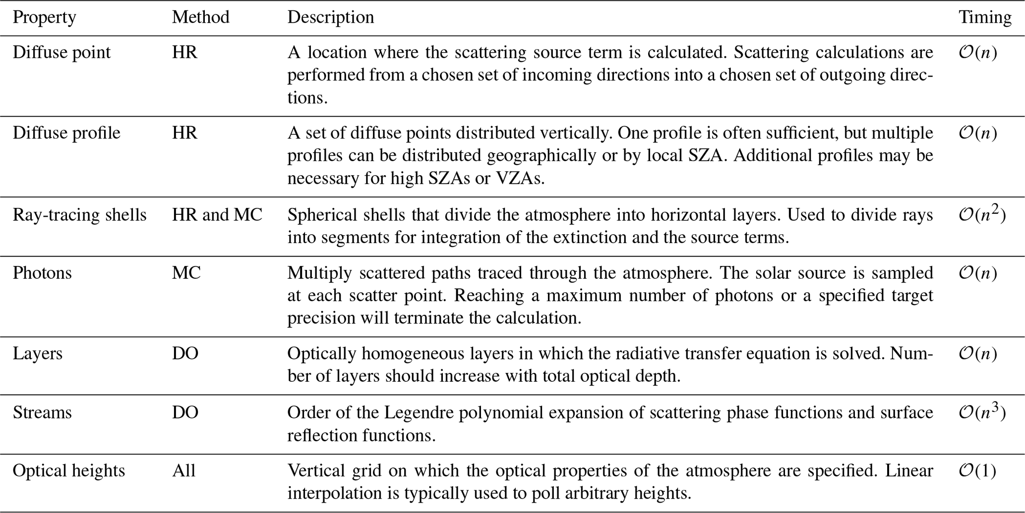
SASKTRAN-DO is the fastest method in SASKTRAN, and with spherical corrections it provides enough accuracy for most nadir-viewing applications, but it is not capable of modeling horizontal inhomogeneities or accounting for the horizontal distribution of the light path. SASKTRAN-HR can model horizontal effects in a fully spherical atmosphere; for example, it has been used to perform two-dimensional limb ozone retrievals with the Ozone Mapping and Profiler Suite Limb Profiler (OMPS-LP) (Zawada et al., 2018). Many lines of sight can be evaluated with little extra computational effort, but currently AMFs must be computed with a finite-difference approximation which is time-consuming for many vertical layers. SASKTRAN-MC can also model horizontal effects, but it requires long computation times to achieve sufficiently high numerical accuracy, and lines of sight must be considered individually. The analysis presented here is scalar, but all three methods are capable of performing polarized radiative transfer calculations. The following section describes the theory, the key definitions and settings (see Table 1), and the recent developments that are relevant for AMF calculations for each method.

Table 1 Summary of SASKTRAN definitions and discretizations for three radiative transfer methods: HR (high resolution, successive orders), MC (Monte Carlo), and DO (discrete ordinates). See Fig. 5 for an illustration of HR properties.

2.1 SASKTRAN-HR

The following is the equation of radiative transfer in a form suitable for the method of successive orders. The radiance $I(\mathit{r},\widehat{\mathbf{\Omega }})$ at position r in direction $\widehat{\mathbf{\Omega }}$ is given by

$$\begin{array}{}\text{(1)}& I(\mathit{r},\widehat{\mathbf{\Omega }})=\sum _{n=\mathrm{1}}^{\mathrm{\infty }}{I}_n(\mathit{r},\widehat{\mathbf{\Omega }}),\end{array}$$

where $I_n(\mathit{r},\widehat{\mathbf{\Omega }})$ is the component of $I(\mathit{r},\widehat{\mathbf{\Omega }})$ that has been scattered n times. It is given by

$$\begin{array}{}\text{(2)}& \begin{array}{rl}{I}_n(\mathit{r},\widehat{\mathbf{\Omega }})& =\underset{s_{\mathrm{1}}}{\overset{\mathrm{0}}{\int }}{J}_n({\mathit{r}}_s,\widehat{\mathbf{\Omega }})k\left({\mathit{r}}_s\right)e^{-{\int }_s^{\mathrm{0}}k\left({\mathit{r}}_t\right)\mathrm{d}t}\mathrm{d}s\\ & +\stackrel{\mathrm{̃}}{I_n}({\mathit{r}}_{s_{\mathrm{1}}},\widehat{\mathbf{\Omega }})e^{-{\int }_{s_{\mathrm{1}}}^{\mathrm{0}}k\left({\mathit{r}}_s\right)\mathrm{d}s},\end{array}\end{array}$$

where k(r) is the total extinction due to scattering and absorption. When refraction is not considered, the path behind r is parameterized by ${\mathit{r}}_s\equiv \mathit{r}+s\widehat{\mathbf{\Omega }}$ with s≤0, and s₁ is defined such that ${\mathit{r}}_{s_{\mathrm{1}}}$ lies on the surface or top of the atmosphere. The nth-order source terms accounting for atmospheric scattering $J_n(\mathit{r},\widehat{\mathbf{\Omega }})$ and surface reflection ${\stackrel{\mathrm{̃}}{I}}_n(\mathit{r},\widehat{\mathbf{\Omega }})$ are given by

$$\begin{array}{}\text{(3a)}& {\displaystyle }{J}_n(\mathit{r},\widehat{\mathbf{\Omega }})& {\displaystyle }={\mathit{\omega }}_{\mathrm{0}}\left(\mathit{r}\right)\underset{\mathrm{4}\mathit{\pi }}{\int }{I}_{n-\mathrm{1}}(\mathit{r},{\widehat{\mathbf{\Omega }}}^{\prime })\overline{p}(\mathit{r},\widehat{\mathbf{\Omega }},{\widehat{\mathbf{\Omega }}}^{\prime })\mathrm{d}{\mathrm{\Omega }}^{\prime },\text{(3b)}& {\displaystyle }{\stackrel{\mathrm{̃}}{I}}_n(\mathit{r},\widehat{\mathbf{\Omega }})& {\displaystyle }=\underset{\mathrm{2}\mathit{\pi }}{\int }{I}_{n-\mathrm{1}}(\mathit{r},{\widehat{\mathbf{\Omega }}}^{\prime })B(\mathit{r},\widehat{\mathbf{\Omega }},{\widehat{\mathbf{\Omega }}}^{\prime })\mathit{\mu }\left({\widehat{\mathbf{\Omega }}}^{\prime }\right)\mathrm{d}{\mathrm{\Omega }}^{\prime },\end{array}$$

for n>1, where ω₀(r) is the single-scattering albedo, $p(\mathit{r},\widehat{\mathbf{\Omega }},{\widehat{\mathbf{\Omega }}}^{\prime })$ is the scattering phase function, $B(\mathit{r},\widehat{\mathbf{\Omega }},{\widehat{\mathbf{\Omega }}}^{\prime })$ is the bidirectional reflectance distribution function (BRDF), and $\mathit{\mu }\left({\widehat{\mathbf{\Omega }}}^{\prime }\right)$ is the cosine of the zenith angle of the incoming direction ${\widehat{\mathbf{\Omega }}}^{\prime }$. The formulation is completed by the single-scatter source terms:

$$\begin{array}{}\text{(4a)}& {\displaystyle }{J}_{\mathrm{1}}(\mathit{r},\widehat{\mathbf{\Omega }})& {\displaystyle }={\mathit{\omega }}_{\mathrm{0}}\left(\mathit{r}\right)F_{\mathrm{0}}{e}^{-{\int }_{s_{\mathrm{2}}}^{\mathrm{0}}k(\mathit{r}+s{\widehat{\mathbf{\Omega }}}_{\mathrm{0}})\mathrm{d}s}p(\mathit{r},\widehat{\mathbf{\Omega }},{\widehat{\mathbf{\Omega }}}_{\mathrm{0}}),\text{(4b)}& {\displaystyle }\stackrel{\mathrm{̃}}{I_{\mathrm{1}}}(\mathit{r},\widehat{\mathbf{\Omega }})& {\displaystyle }=F_{\mathrm{0}}{e}^{-{\int }_{s_{\mathrm{2}}}^{\mathrm{0}}k(\mathit{r}+s{\widehat{\mathbf{\Omega }}}_{\mathrm{0}})\mathrm{d}s}B(\mathit{r},\widehat{\mathbf{\Omega }},{\widehat{\mathbf{\Omega }}}_{\mathrm{0}})\mathit{\mu }\left({\widehat{\mathbf{\Omega }}}_{\mathrm{0}}\right),\end{array}$$

where F₀ is the magnitude of the top-of-atmosphere solar irradiance, ${\widehat{\mathbf{\Omega }}}_{\mathrm{0}}$ is its direction, and s₂ is defined such that $\mathit{r}+s_{\mathrm{2}}{\widehat{\mathbf{\Omega }}}_{\mathrm{0}}$ is at top of the atmosphere. The diffuse radiation field is solved one order of scatter at a time using the results from one order to calculate the next.

The radiation field is five-dimensional, with three spatial and two directional coordinates, but symmetries around the solar zenith reduce the dimensionality to four for certain atmospheric and surface configurations, including common cases such as a horizontally homogeneous spherical shell atmosphere and Lambertian surface. The radiation field is discretized by selecting so-called diffuse points throughout the atmosphere: locations where the radiance is scattered from a set of incoming directions into a set of outgoing directions. One vertical profile of diffuse points, called a diffuse profile, is often sufficient for scenes with small or moderate zenith angles and a horizontally homogeneous atmosphere. Incoming radiances at diffuse points are computed with explicit ray tracing, dividing the rays into segments according to their intersections with a set of spherical shells, and integrating the extinctions and the source terms. A key advantage of this method is that it computes the full multiple scatter diffuse field, so radiances (and therefore AMF profiles) for any number of lines of sight can be computed with very little extra cost by simply integrating along all lines of sight at the end of the computation. Table 1 summarizes the terminology used to describe the key discretizations used by SASKTRAN-HR.

SASKTRAN-HR has built-in approximate analytical weighting functions (Zawada et al., 2015) which approximate the derivative of the radiance with respect to number density grid points, but they have been found to lack the accuracy required for AMF calculations, so a finite-difference scheme is adopted. More precise placement options for optical properties, ray-tracing shells, and diffuse points have been added to facilitate accurate finite-difference calculations in one or more dimensions.

2.2 SASKTRAN-MC

SASKTRAN-MC applies the backwards Monte Carlo method to the radiative transfer equation separated by order of scatter (Eqs. 2 through 4), taking random samples of the radiance by explicitly tracing backwards rays that originate at the instrument, are propagated and scattered throughout the atmosphere, and terminate at the sun (Zawada et al., 2015). In generalized notation, the radiance can be given by

$$\begin{array}{}\text{(5)}& I(\mathit{r},\widehat{\mathbf{\Omega }})=\sum _{n=\mathrm{1}}^{\mathrm{\infty }}\underset{D_n}{\int }{f}_n\left({\mathit{x}}_n\right)\mathrm{d}{\mathit{x}}_n,\end{array}$$

where x_n is any parameterization of a light path with n scattering or reflection events, D_n is the space of all such paths ending at position r and direction $\widehat{\mathbf{\Omega }}$, and f_n(x_n)dx_n is the radiance contribution from the infinitesimal group of light paths dx_n. The radiance and its variance are estimated by Monte Carlo integration: taking samples x_nk from probability density function p_n(x_n) via backwards ray tracing and computing the mean and the variance of $f_n\left({\mathit{x}}_{nk}\right)/p_n\left({\mathit{x}}_{nk}\right)$. The parameterization x_n has 3n−2 degrees of freedom; for example, if the SASKTRAN-MC formulation (Zawada et al., 2015) used this notation, x_k would consist of n path lengths, n−1 scattering angles, and n−1 rotation angles.

The Monte Carlo method does not rely on the discretization of the diffuse field and is therefore effective for validating the placement of diffuse points and the choice of incoming and outgoing angular grids in SASKTRAN-HR. As indicated in Table 1, optical heights and ray-tracing shells still need to be chosen. This method is flexible and accurate and can be run to arbitrary precision, but high-precision results require large computation times, and unlike SASKTRAN-HR each line of sight must be considered individually. Therefore it is not feasible for extensive AMF table generation, but it is ideal for validation or for small studies. The calculation of AMFs and their variances via explicit ray tracing has been recently implemented in SASKTRAN-MC. Further details can be found in Sect. 3.6.

2.3 SASKTRAN-DO

The following is the equation of radiative transfer in a form suitable for the method of discrete ordinates, as developed for LIDORT (Linearized Discrete Ordinate Radiative Transfer) in Spurr et al. (2001):

$$\begin{array}{}\text{(6)}& \mathit{\mu }{\displaystyle \frac{\mathrm{d}I(\mathit{\tau },\mathit{\mu },\mathit{\varphi })}{\mathrm{d}\mathit{\tau }}}=I(\mathit{\tau },\mathit{\mu },\mathit{\varphi })-J(\mathit{\tau },\mathit{\mu },\mathit{\varphi }),\end{array}$$

where the vertical coordinate τ is optical depth from the top of the atmosphere, and direction is represented by the absolute value of the zenith cosine μ and the azimuth ϕ. The source term J is given by

$$\begin{array}{}\text{(7)}& \begin{array}{rl}J(\mathit{\tau },\mathit{\mu },\mathit{\varphi })& =J_{\text{ext}}(\mathit{\tau },\mathit{\mu },\mathit{\varphi })\\ & +{\mathit{\omega }}_{\mathrm{0}}\left(\mathit{\tau }\right)\underset{\mathrm{4}\mathit{\pi }}{\int }I(\mathit{\tau },{\widehat{\mathbf{\Omega }}}^{\prime })p(\mathit{\tau },\widehat{\mathbf{\Omega }},{\widehat{\mathbf{\Omega }}}^{\prime })\mathrm{d}{\widehat{\mathbf{\Omega }}}^{\prime },\end{array}\end{array}$$

where the first term J_ext consists of thermal emissions and scattering of the direct solar beam, and the second term is the contribution from multiple scattering. The solution to Eqs. (6) and (7) in a homogeneous slab is computed by expanding the radiance I in a Fourier cosine series in azimuth angle, expanding the phase function p in a series of Legendre polynomials in the cosine of the scatter angle, discretizing μ by applying Gauss–Legendre quadrature to the integral in the multiple scattering source term, and solving the resulting set of linear first-order differential equations in τ.

SASKTRAN-DO is a separate module within the SASKTRAN framework which uses the discrete ordinates technique to solve the radiative transfer equation in a plane-parallel atmosphere consisting of homogeneous vertical layers. The model is optionally polarized and uses a pseudo-spherical correction which initializes the technique with the solar beam attenuated in a fully spherical atmosphere. The model can calculate analytic derivatives with respect to atmospheric parameters, including number density grid points, which produces weighting functions of the same form as SASKTRAN-HR.

Spherical line-of-sight corrections have recently been added to SASKTRAN-DO. Here, the single-scatter source is calculated exactly in a spherical atmosphere assuming a linear variation in extinction between layer boundaries. The multiple-scatter source is approximated by multiple executions of the discrete ordinates technique at a user-specified number of solar zenith angles along the line of sight. The observed radiance is then calculated by integrating these source terms in a spherical atmosphere. The spherical mode retains the ability to compute analytic derivatives but is currently only capable of scalar calculations. The technique is similar to that of the newly released VLIDORT-QS (Spurr et al., 2022). Key parameters controlling accuracy are described in Table 1.

3 Air mass factors

The following section presents the theoretical basis for AMFs computed with SASKTRAN: through finite-difference weighting functions with SASKTRAN-HR, through built-in weighting functions with SASKTRAN-DO, and through explicit ray tracing with SASKTRAN-MC. The traditional framework, based on homogeneous atmospheric layers, is expanded to allow for alternative vertical discretizations, such as the linear interpolation used by SASKTRAN, and the introduction of horizontal discretizations.

3.1 Total AMF

The purpose of AMF in DOAS-style retrievals is to transform the slant column density (SCD), a measure of the state of the atmosphere that is heavily coupled with the measurement setup, to the vertical column density (VCD), a function of atmosphere alone. The AMF is a function of the instrument and sun position, as well as scene information such as surface albedo and cloud cover. For measurements of scattered light, there are a variety of subtle differences between definitions of the SCD and the AMF, depending on different approximations or different variations of the DOAS method. See, for example, Palmer et al. (2001) for one of the earliest popular AMF formulations, Platt and Stutz (2008) for a comprehensive discussion on DOAS methods, and Rozanov and Rozanov and Rozanov (2010) for a detailed look at the subtleties associated with DOAS applied to multiply scattered radiation.

For the following work, the AMF (A), the SCD (S), and the VCD (V) are defined as

$$\begin{array}{}\text{(8)}& A\equiv {\displaystyle \frac{S}{V}}\equiv {\displaystyle \frac{{\int }_{L}n\left(l\right)\mathrm{d}l}{{\int }_{\mathrm{0}}^{H}n\left(z\right)\mathrm{d}z}},\end{array}$$

where n(z) is the number density of the target species, integration over z is along the local vertical from the surface 0 to the top of the atmosphere H, and integration over l is along the so-called slant path L, which is effectively the average path history of all the light that is captured by the instrument (see Fig. 1). More specifically, an integral along the slant path is defined here as the radiance-weighted average of the integrals along all contributing light paths. Using the notation of Eq. (5), it can be described by

$$\begin{array}{}\text{(9)}& S=\underset{L}{\int }n\left(l\right)\mathrm{d}l\equiv {\displaystyle \frac{{\sum }_{n=\mathrm{1}}^{\mathrm{\infty }}{\int }_{D_n}{f}_n\left({\mathit{x}}_n\right)\left({\int }_{C\left({\mathit{x}}_n\right)}n\left(s\right)\mathrm{d}s\right)\mathrm{d}{\mathit{x}}_n}{{\sum }_{n=\mathrm{1}}^{\mathrm{\infty }}{\int }_{D_n}{f}_n\left({\mathit{x}}_n\right)\mathrm{d}{\mathit{x}}_n}},\end{array}$$

where integration over s is along the path C(x_n) represented by parameterization x_n.

Equation (9) is suitable for AMF calculations with SASKTRAN-MC via ray tracing, which is discussed in Sect. 3.6. Section 3.2 through 3.5 connect the AMF definition in Eq. (8) to derivatives of radiance with respect to optical parameters, which is suitable for AMF calculations with SASKTRAN-HR and SASKTRAN-MC.

3.2 Continuous AMF

Consider the quantity dl in Eqs. (8) and (9): it represents the effective length of the average contributing light path within the infinitesimal horizontal layer dz. We define the continuous AMF profile,

$$\begin{array}{}\text{(10)}& A\left(z\right)={\displaystyle \frac{\mathrm{d}l}{\mathrm{d}z}},\end{array}$$

describing the enhancement of the slant path compared to the vertical path as a function of altitude. Note that this is now decoupled from the absorber profile n(z) in Eq. (8) but still depends weakly on the absorber profile through the radiance contribution f_n(x_n)dx_n in Eq. (9). This dependence is typically considered to be negligible under the weak absorber approximation.

AMFs are closely related to derivatives of optical properties, often called weighting functions. Following Rozanov and Rozanov (2010), the continuous AMF profile A(z) is equal to the negative of the functional derivative defined by

$$\begin{array}{}\text{(11)}& \begin{array}{rl}& \int {\displaystyle \frac{\partial \ln I}{\partial k}}\left(z\right)\mathit{\varphi }\left(z\right)\mathrm{d}z=\\ & \underset{\mathrm{\Delta }k\to \mathrm{0}}{lim}{\displaystyle \frac{\ln I\left[k\right(z)+\mathrm{\Delta }k\mathit{\varphi }(z\left)\right]-\ln I\left[k\right(z\left)\right]}{\mathrm{\Delta }k}},\end{array}\end{array}$$

where I[k(z)] is the measured radiance due to absorber extinction profile k(z)=n(z)σ(z), σ(z) is the absorption cross section, Δk is a perturbation with units of extinction, and ϕ(z) is an arbitrary unitless function. This equivalence is evident when linearizing the radiance due to a perturbed extinction profile about k(z),

$$\begin{array}{}\text{(12)}& \begin{array}{rl}& \ln I\left[k\right(z)+\mathrm{\Delta }k\mathit{\varphi }(z\left)\right]=\ln I\left[k\right(z\left)\right]\\ & +\underset{\mathrm{0}}{\overset{H}{\int }}{\displaystyle \frac{\partial \ln I}{\partial k}}\left(z\right)\mathrm{\Delta }k\mathit{\varphi }\left(z\right)\mathrm{d}z+\mathcal{O}\left(\mathrm{\Delta }{k}^{\mathrm{2}}\right),\end{array}\end{array}$$

and comparing it to the use of the Beer–Lambert law to describe the difference between these radiances using the continuous AMF (Eq. 10) as a change of variables for the slant path integration,

$$\begin{array}{}\text{(13)}& \begin{array}{rl}\ln I\left[k\right(z)& +\mathrm{\Delta }k\mathit{\varphi }\left(z\right)]-\ln I[k\left(z\right)]\\ & =-\underset{L}{\int }\mathrm{\Delta }k\mathit{\varphi }\left(l\right)\mathrm{d}l=-\underset{\mathrm{0}}{\overset{H}{\int }}\mathrm{\Delta }k\mathit{\varphi }\left(z\right)A\left(z\right)\mathrm{d}z.\end{array}\end{array}$$

This equivalence is convenient; AMFs, which contain information about the distribution of the light path, can be computed from derivatives of radiance with respect to extinction. It is also intuitive, with denser and longer light paths resulting in a larger response from the radiance to a perturbation in extinction.

3.3 Box-AMF

In practice the radiative transfer equation cannot be solved with a continuous vertical coordinate, so the absorber profile n(z) and the rest of the optical properties must be discretized. The result is altitude-dependent AMF quantities which we will call box-AMFs, though they also go by other names such as scattering weights. We assume the absorber profile n(z) is discretized according to

$$\begin{array}{}\text{(14)}& n\left(z\right)=\sum _j{n}_j{\mathit{\varphi }}_j\left(z\right),\end{array}$$

where the discretizing functions ϕ_j(z) are constrained by

$$\begin{array}{}\text{(15)}& \sum _j{\mathit{\varphi }}_j\left(z\right)=\left\{\begin{array}{ll}\mathrm{1}& \mathrm{0}\le z\le H\\ \mathrm{0}& \text{else}\end{array}\right.,\end{array}$$

and an effective layer thickness is defined by

$$\begin{array}{}\text{(16)}& \mathrm{\Delta }{z}_j\equiv \underset{\mathrm{0}}{\overset{H}{\int }}{\mathit{\varphi }}_j\left(z\right)\mathrm{d}z.\end{array}$$

ϕ_j(z) are typically boxes, corresponding to a model with constant horizontal layers, or triangles, corresponding to a model with linear interpolation on the vertical coordinate. Using the continuous AMF from Eq. (10) as a change of variables, we rewrite the total AMF from Eq. (8) as

$$\begin{array}{}\text{(17)}& A={\displaystyle \frac{S}{V}}={\displaystyle \frac{{\int }_{\mathrm{0}}^{H}n\left(z\right)A\left(z\right)\mathrm{d}z}{{\int }_{\mathrm{0}}^{H}n\left(z\right)\mathrm{d}z}},\end{array}$$

and we plug in the discretized absorber profile from Eq. (14), returning

$$\begin{array}{}\text{(18)}& A={\displaystyle \frac{{\sum }_j{n}_j{\int }_{\mathrm{0}}^H{\mathit{\varphi }}_j\left(z\right)A\left(z\right)\mathrm{d}z}{{\sum }_j{n}_j{\int }_{\mathrm{0}}^H{\mathit{\varphi }}_j\left(z\right)\mathrm{d}z}}.\end{array}$$

This motivates the definition of the partial SCD,

$$\begin{array}{}\text{(19)}& s_j\equiv n_j\underset{\mathrm{0}}{\overset{H}{\int }}{\mathit{\varphi }}_j\left(z\right)A\left(z\right)\mathrm{d}z,\end{array}$$

the partial VCD,

$$\begin{array}{}\text{(20)}& v_j\equiv n_j\underset{\mathrm{0}}{\overset{H}{\int }}{\mathit{\varphi }}_j\left(z\right)\mathrm{d}z=n_j\mathrm{\Delta }{z}_j,\end{array}$$

and the box-AMF,

$$\begin{array}{}\text{(21)}& a_j\equiv {\displaystyle \frac{s_j}{v_j}}={\displaystyle \frac{\mathrm{1}}{\mathrm{\Delta }{z}_j}}\underset{\mathrm{0}}{\overset{H}{\int }}{\mathit{\varphi }}_j\left(z\right)A\left(z\right)\mathrm{d}z.\end{array}$$

See Fig. 1 for an illustration of these quantities. With these definitions, the total AMF is computed according to

$$\begin{array}{}\text{(22)}& A={\displaystyle \frac{S}{V}}={\displaystyle \frac{{\sum }_j{s}_j}{{\sum }_j{v}_j}}={\displaystyle \frac{{\sum }_j{v}_j{a}_j}{{\sum }_j{v}_j}}.\end{array}$$

As long as the discretizing functions ϕ_j(z) are sufficiently narrow, the box-AMFs a_j are insensitive to the absorber profile, allowing them to be tabulated and used for scenes with arbitrary absorber profiles v_j.

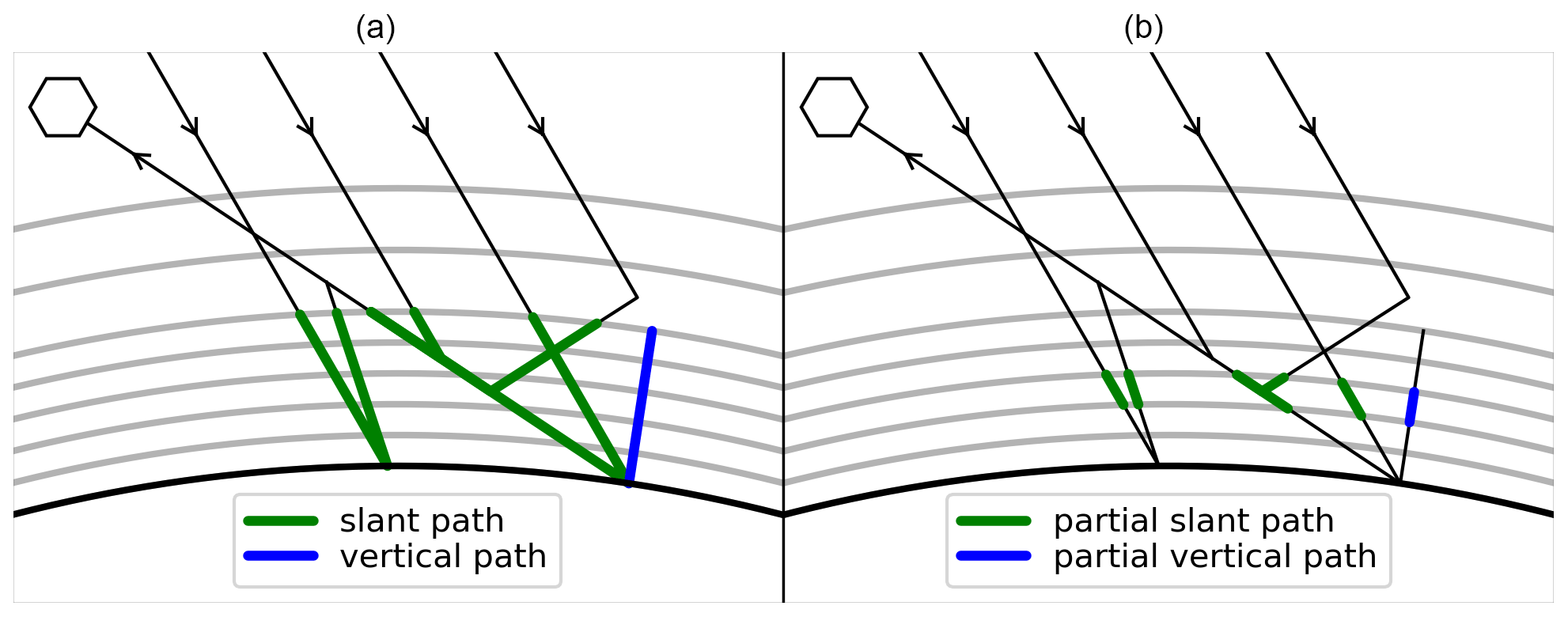
Figure 1 Simplified representation of the paths used to define the total SCD (S) and the total VCD (V) (a) as well as the partial SCD (s_j) and the partial VCD (v_j) (b). VCDs are number density integrals along the blue paths, and SCDs are radiance-weighted number density integrals along all green paths. The total AMF (A) is the ratio of the total SCD to the total VCD, and the box-AMF (a_j) is the ratio of the partial SCD to the partial VCD.

3.4 Multidimensional AMF

This framework can be generalized to be compatible with different coordinate systems in two or three dimensions, permitting box-AMFs which characterize the horizontal distribution of the measured light path in addition to the vertical. In three dimensions, the total SCD is given by

$$\begin{array}{}\text{(23)}& S=\iiint n\left(\mathit{x}\right)A\left(\mathit{x}\right)\mathrm{d}V,\end{array}$$

where x is a parameterization of three-dimensional space, dV is the volume element spanning from x to x+dx, A(x)dV is the length of the slant path that is contained within this volume, and integration occurs over the entire defined atmosphere. Since we are ultimately interested in retrieving vertical columns, we will insist that one component of x is vertical and furthermore that the discretization of n(x) be organized into vertical columns. Let x₁ and x₂ be horizontal components, such as Cartesian coordinates in a plane-parallel atmosphere or orthogonal angles in a spherical atmosphere, and let x₃ be a vertical coordinate, such as altitude or pressure. Let the number density n(x) be discretized into N columns by the horizontal shape functions ψ_i(x₁,x₂) such that

$$\begin{array}{}\text{(24)}& \sum _{i=\mathrm{1}}^N{\mathit{\psi }}_i(x_{\mathrm{1}},x_{\mathrm{2}})=\mathrm{1}.\end{array}$$

Let the vertical shape functions ϕ_ij(x₃) discretize column i into N_i layers constrained by

$$\begin{array}{}\text{(25)}& \sum _{j=\mathrm{1}}^{N_i}{\mathit{\varphi }}_{ij}\left(x_{\mathrm{3}}\right)=\mathrm{1},\end{array}$$

such that the effective thickness of layer j in column i is given by

$$\begin{array}{}\text{(26)}& \mathrm{\Delta }{z}_{ij}=\int {\mathit{\varphi }}_{ij}\left(x_{\mathrm{3}}\right)\mathrm{d}L,\end{array}$$

where dL is the length element spanning from x₃ to x₃+dx₃. The full number density field n(x) is then represented by

$$\begin{array}{}\text{(27)}& n\left(\mathit{x}\right)=\sum _{i=\mathrm{1}}^N\sum _{j=\mathrm{1}}^{N_i}{n}_{ij}{\mathit{\psi }}_i(x_{\mathrm{1}},x_{\mathrm{2}}){\mathit{\varphi }}_{ij}\left(x_{\mathrm{3}}\right).\end{array}$$

We define the partial SCD,

$$\begin{array}{}\text{(28)}& s_{ij}=n_{ij}\iiint {\mathit{\psi }}_i(x_{\mathrm{1}},x_{\mathrm{2}}){\mathit{\varphi }}_{ij}\left(x_{\mathrm{3}}\right)A(x_{\mathrm{1}},x_{\mathrm{2}},x_{\mathrm{3}})\mathrm{d}V,\end{array}$$

the partial VCD,

$$\begin{array}{}\text{(29)}& v_{ij}=n_{ij}\mathrm{\Delta }{z}_{ij},\end{array}$$

and the box-AMF,

$$\begin{array}{}\text{(30)}& a_{ij}={\displaystyle \frac{\mathrm{1}}{\mathrm{\Delta }{z}_{ij}}}\iiint {\mathit{\psi }}_j(x_{\mathrm{1}},x_{\mathrm{2}}){\mathit{\varphi }}_{ij}\left(x_{\mathrm{3}}\right)A(x_{\mathrm{1}},x_{\mathrm{2}},x_{\mathrm{3}})\mathrm{d}V.\end{array}$$

Defining the total VCD of column i,

$$\begin{array}{}\text{(31)}& V_i\equiv \sum _{j=\mathrm{1}}^{N_i}{v}_{ij},\end{array}$$

we seek the total AMF A_i that would be used to retrieve V_i:

$$\begin{array}{}\text{(32)}& A_i\equiv {\displaystyle \frac{S}{V_i}}={\displaystyle \frac{{\sum }_{i^{\prime }=\mathrm{1}}^N{\sum }_{j=\mathrm{1}}^{N_{i^{\prime }}}{s}_{i^{\prime }j}}{{\sum }_{j=\mathrm{1}}^{N_i}{v}_{ij}}}={\displaystyle \frac{{\sum }_{i^{\prime }=\mathrm{1}}^N{\sum }_{j=\mathrm{1}}^{N_{i^{\prime }}}{v}_{i^{\prime }j}{a}_{i^{\prime }j}}{{\sum }_{j=\mathrm{1}}^{N_i}{v}_{ij}}}.\end{array}$$

3.5 AMFs via weighting functions

Here we derive the relation between box-AMFs and discrete weighting functions. Using the equality of continuous weighting functions and AMF profiles (Eqs. 12 and 13) the box-AMF (Eq. 21) can be written as

$$\begin{array}{}\text{(33)}& a_j={\displaystyle \frac{s_j}{v_j}}=-{\displaystyle \frac{\mathrm{1}}{\mathrm{\Delta }{z}_j}}\underset{\mathrm{0}}{\overset{H}{\int }}{\mathit{\varphi }}_j\left(z\right){\displaystyle \frac{\partial \ln I}{\partial k}}\left(z\right)\mathrm{d}z.\end{array}$$

Applying the functional derivative definition (see Eq. 11), we get

$$\begin{array}{}\text{(34)}& a_j=-{\displaystyle \frac{\mathrm{1}}{\mathrm{\Delta }{z}_j}}\underset{\mathrm{\Delta }k\to \mathrm{0}}{lim}{\displaystyle \frac{\ln I\left[k\right(z)+\mathrm{\Delta }k{\mathit{\varphi }}_j(z\left)\right]-\ln I\left[k\right(z\left)\right]}{\mathrm{\Delta }k}},\end{array}$$

which is nearly equivalent to

$$\begin{array}{}\text{(35)}& a_j=-{\displaystyle \frac{\mathrm{1}}{\mathrm{\Delta }{z}_j}}\underset{\mathrm{\Delta }n\to \mathrm{0}}{lim}{\displaystyle \frac{\ln I\left[n\right(z)+\mathrm{\Delta }n{\mathit{\varphi }}_j(z\left)\right]-\ln I\left[n\right(z\left)\right]}{{\mathit{\sigma }}_j\mathrm{\Delta }n}},\end{array}$$

where σ_j is the absorption cross section corresponding to ϕ_j(z). The difference between Eqs. (34) and (35) is a slight change in perturbation shape due to the vertical structure of σ(z) which varies with temperature. This change is assumed to be negligible, as vertical gradients of absorption cross sections are typically small and ϕ_j(z) confines the changes to a small vertical region. In a constant-layer model, there is no change, as the temperature and therefore the cross section are constant within the layer. Applying a perturbation with shape ϕ_j(z) to the profile n(z) is equivalent to perturbing the parameter n_j. Therefore, the limit in Eq. (35) can be rewritten as follows:

$$\begin{array}{}\text{(36)}& a_j=-{\displaystyle \frac{\mathrm{1}}{{\mathit{\sigma }}_j\mathrm{\Delta }{z}_{j}I}}{\displaystyle \frac{\partial I}{\partial n_j}},\end{array}$$

which now contains the derivative of radiance with respect to number density grid points; this is the form of the weighting functions returned by SASKTRAN-HR and SASKTRAN-DO. Two-dimensional box-AMFs in SASKTRAN-HR are similarly computed according to

$$\begin{array}{}\text{(37)}& a_{ij}=-{\displaystyle \frac{\mathrm{1}}{{\mathit{\sigma }}_{ij}\mathrm{\Delta }{z}_{ij}I}}{\displaystyle \frac{\partial I}{\partial n_{ij}}}.\end{array}$$

These results were found to remain insensitive to a variety of perturbation shapes. For example, using a rectangular ϕ_j(z) to compute v_j, which is how it is typically defined in the literature, while using a triangular perturbation to compute a_j, which is more compatible with SASKTRAN, was found to still produce accurate results. Some of the early tables discussed in Sect. 5 employed this strategy using a triangular perturbation contained within each AMF layer to compute the box-AMF. This required two ray-tracing shells and two diffuse points per layer, which drove up the computation time significantly when additional AMF layers were required due to the 𝒪(n²) dependence on the number of ray-tracing shells. This motivated the use of a constant-layer atmosphere representation, which permitted the use of rectangular perturbations, requiring only one ray-tracing shell and one diffuse point per layer. This strategy resulted in negligible changes to the box-AMFs and was therefore used for the SASKTRAN-HR box-AMFs presented in Sect. 4.

3.6 AMFs via ray tracing

A ray-tracing method for computing box-AMFs with SASKTRAN-MC was implemented to be used as validation for the weighting function AMFs. Consider the partial SCD definition in Eq. (19); if the slant path integration A(z)dz is replaced with the definition from Eq. (9), the partial SCD becomes

$$\begin{array}{}\text{(38)}& s_j={\displaystyle \frac{{\sum }_{n=\mathrm{1}}^{\mathrm{\infty }}{\int }_{D_n}{f}_n\left({\mathit{x}}_n\right)\left(n_j{\int }_{C\left({\mathit{x}}_n\right)}{\mathit{\varphi }}_j\left(s\right)\mathrm{d}s\right)\mathrm{d}{\mathit{x}}_n}{{\sum }_{n=\mathrm{1}}^{\mathrm{\infty }}{\int }_{D_n}{f}_n\left({\mathit{x}}_n\right)\mathrm{d}{\mathit{x}}_n}}.\end{array}$$

As described in Sect. 2.2, the radiance and its variance are computed by sampling x_n via backwards ray tracing. To calculate the partial SCD s_j (and therefore the box-AMF a_j), the same ray tracing is used to simultaneously estimate the integrals in the denominator (the radiance, as before) and the numerator of Eq. (38), explicitly integrating the number density along each traced light path. The variance of a_j is estimated by computing the variance and covariance of the two integrals, then using a first-order Taylor expansion to approximate the variance of their ratio.

4 AMF comparisons

4.1 SASKTRAN-MC vs. SASKTRAN-HR

The following section presents a series of comparisons between box-AMF profiles generated using SASKTRAN-HR and SASKTRAN-MC. The 1976 US Standard Atmosphere (Dubin et al., 1976) was used for air density, temperature, pressure, and ozone density profiles, and a typical NO₂ density profile was taken from a 1-year global tropospheric chemistry simulation performed using the Goddard Earth Observing System Model version 5 Earth system model (GEOS-5 ESM) with the GEOS-Chem chemical module (G5NR-chem) (Hu et al., 2018). No aerosols were included. Computations were performed at 440 nm, a typical value for AMFs for NO₂ retrievals, and box-AMF layers of thickness 500 m were defined up to 50 km. All computations used ray-tracing shells with 500 m spacing up to 50 km, matching the AMF layers, and with 1 km spacing up to 85 km, the top of the defined atmosphere. All calculations were carried out to 50 orders of scattering.

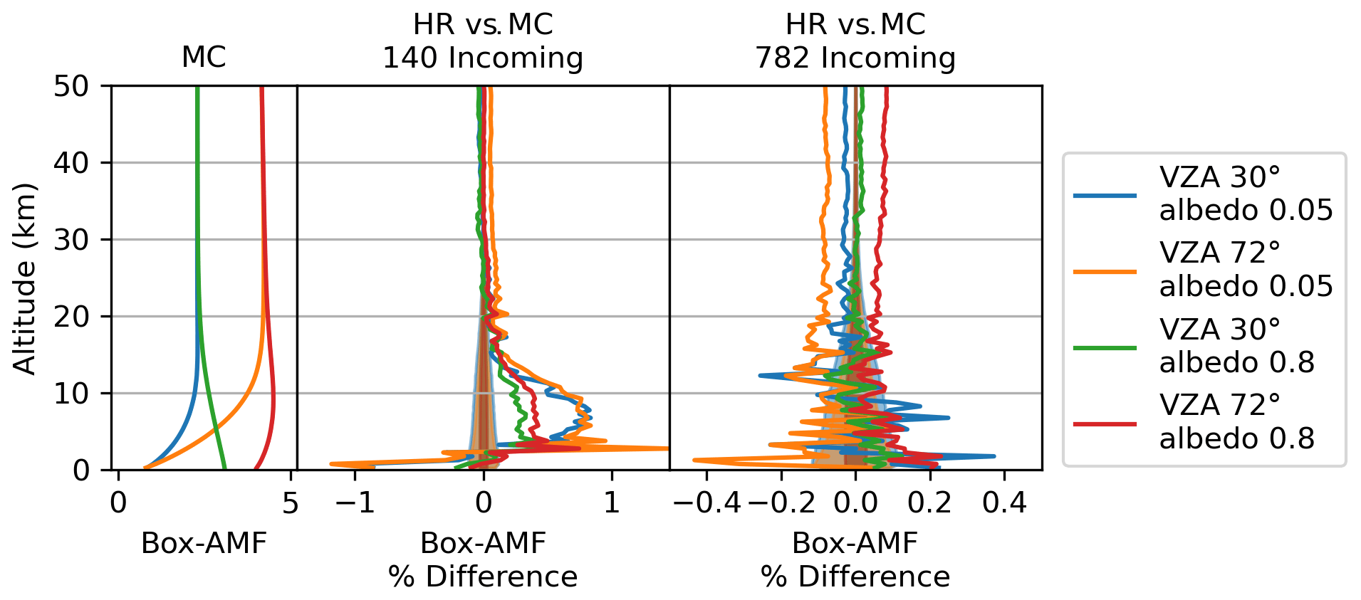
Figure 2 Box-AMF comparison between SASKTRAN-MC and SASKTRAN-HR with a SZA of 30^∘, with two values for the VZA and two values for the surface albedo. The shaded region shows the uncertainty in the SASKTRAN-MC box-AMFs after 10⁷ traced photon paths.

In Fig. 2, the SASKTRAN-HR box-AMFs were computed for moderate geometries which would be commonly found in nadir retrieval products, with a low SZA and a typical range of VZAs. They have been computed twice: once with typical resolutions and once with high resolutions for the diffuse field. A single diffuse profile was used for both computations, with one diffuse point placed just above the surface and one diffuse point placed in the center of each ray-tracing layer. The first computation used 140 incoming directions per diffuse point (see Fig. 5). The result agrees with SASKTRAN-MC within just over 1 %. Calculations were done at surface albedos of 0.05 and 0.8; larger percent errors are observed at the lower albedo in Fig. 2, but this is a consequence of lower AMFs, not higher errors.

Inadequate resolution in the downward and horizontal incoming diffuse field was found to be responsible for most of the discrepancy. In the second computation, the agreement was brought down to within 0.4 % by quadrupling the zenith resolutions in the downward and horizon regions and doubling the azimuth resolution. This resulted in a total of 782 incoming directions per diffuse point (see Fig. 5). Increasing resolution in the upward-facing zenith region was found not to bring any improvement.

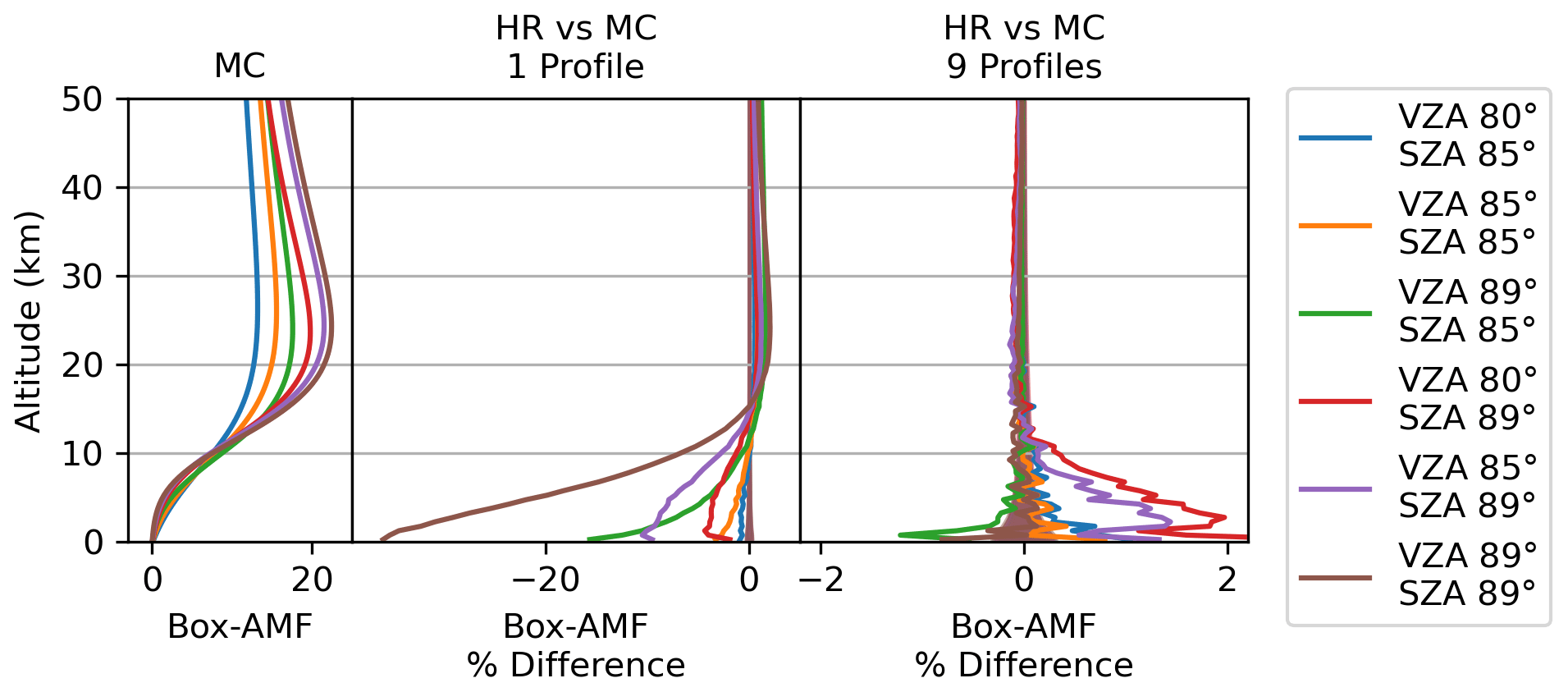
Figure 3 Box-AMF comparison between SASKTRAN-MC and SASKTRAN-HR at extreme geometries with the sun low and with shallow lines of sight. Only one surface albedo (0.05) is considered, but these results are insensitive to surface albedo due to the long light paths.

Figure 3 explores more extreme geometries, with large solar and viewing zenith angles that would not be considered in a typical nadir retrieval product. Significant errors are introduced by the use of a single diffuse profile due to the larger range of SZAs seen along the long, shallow lines of sight. Using nine diffuse profiles, spanning this range of SZAs, was sufficient to bring significant improvement for the configurations shown in Fig. 3. Note that these comparisons are done assuming horizontal homogeneity in the atmosphere; the multiple diffuse profiles account for geometric effects, not atmospheric effects such as photochemical changes in NO₂ with SZA. The remaining difference does not appear to respond to increases in HR resolutions, which are already approaching their practical limit. It is perhaps a limitation of the finite-difference approximation or some subtle difference between method-specific configurations which is amplified by the long light paths in the most extreme geometries.

Results for multiple wavelengths spanning a large range of geometries are presented in Fig. 4. Wavelengths were chosen to match common retrievals spanning a wide range of the visible spectrum, with 330 nm which is typical for formaldehyde retrievals, 440 nm for NO₂, and 600 nm for ozone retrievals using the Chappuis absorption band. The phenomena explored in Figs. 2 and 3 are visible; increasing the diffuse resolution is seen to improve agreement for small to moderate zenith angles, and adding diffuse profiles shows improved agreement for larger zenith angles. The effect of adding diffuse profiles clearly varies with wavelength; at 600 nm where multiple scattering is less important, the difference is reduced, but at 330 nm multiple profiles are shown to be necessary for a larger range of SZAs and VZAs. Even with the increase in diffuse profiles and incoming directions, discrepancies greater than 2 % remain for SZA 89^∘ at 330 and 440 nm. This is due to the proximity of the solar terminator to the ground pixel at such an extreme SZA, in combination with strong contributions from multiple scattering. Under these conditions the solar transmission table, which tabulates the intensity of the direct solar beam as a function of altitude and SZA, would require higher resolutions to accurately capture this discontinuity.

Figure 4 Box-AMF comparisons between SASKTRAN-MC and SASKTRAN-HR.

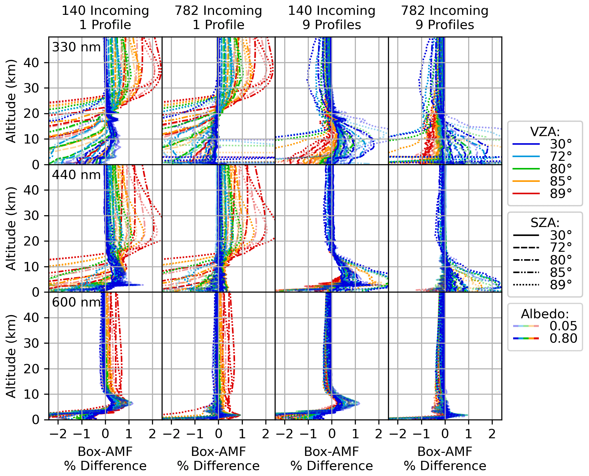
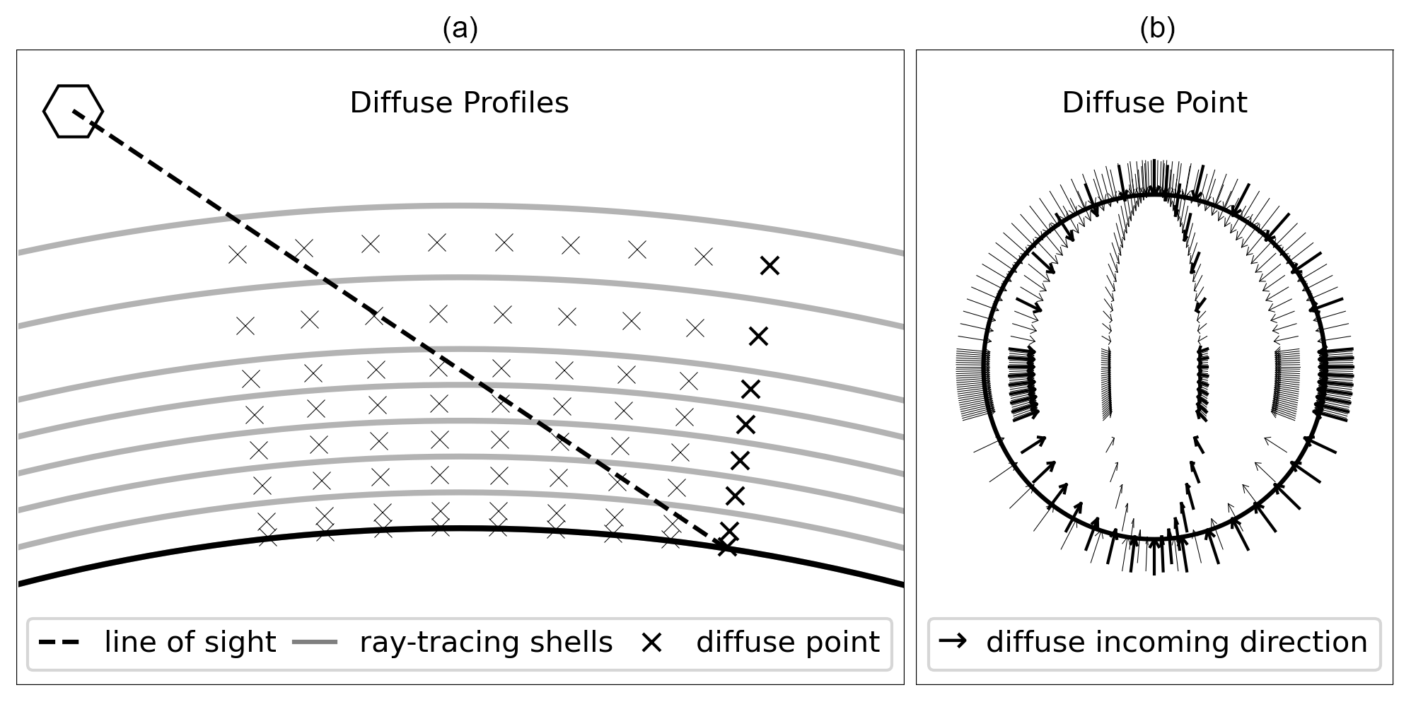
Figure 5 Illustration of the four SASKTRAN-HR configurations used for comparisons with SASKTRAN-MC (Figs. 2 through 4). The single diffuse profile is placed over the ground intersection, and the nine profiles are spread across the range of SZAs along the line of sight. For each diffuse point, incoming zenith angles are distributed uniformly within three regions, with 6 (24) intervals above the horizon region (downward facing), 8 (32) intervals in the horizon region (within 10^∘ of the horizon), and 10 intervals below the horizon region (upward-facing). With two vertical directions and 6 (12) azimuth angles, the total number of diffuse incoming directions is 140 (782). The atmosphere in (a) has a reduced number of ray-tracing shells and diffuse point altitudes.

4.2 SASKTRAN-MC vs. SASKTRAN-DO

The following section examines the accuracy of the pseudo-spherical discrete ordinates solution under the same set of conditions. The following computations used 16 streams in the full space and divide the atmosphere into 250 m layers. The spherical line-of-sight correction computes the diffuse field at five SZAs along the line of sight. The results are displayed in Fig. 6.

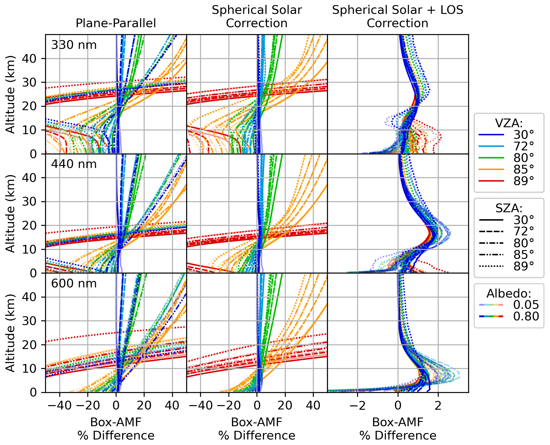
Figure 6 Box-AMF comparisons between SASKTRAN-MC and SASKTRAN-DO. Note that the x-axis scale changes in the rightmost column.

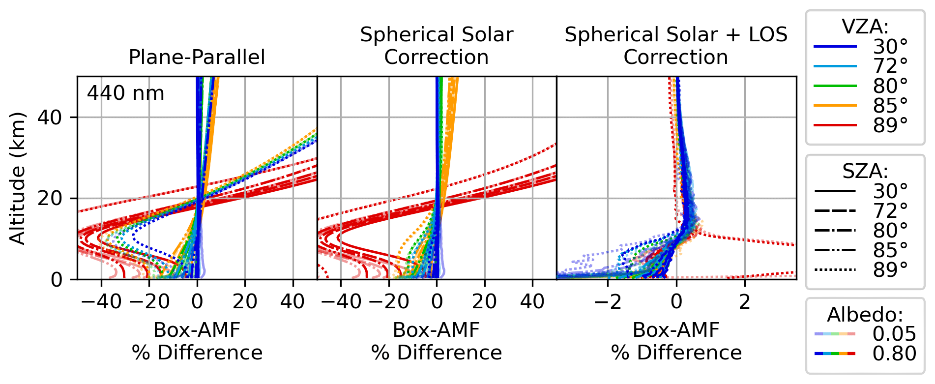
The effect of the solar spherical correction in Fig. 6 is subtle but visible, correcting cases with low VZA and high SZA (see the blue and green transparent lines in the leftmost column compared to the middle). The addition of a spherical line-of-sight correction dramatically improves cases with large VZAs. With these two corrections, the discrepancy is brought to within roughly 3 %. This discrepancy is only weakly dependent on geometry, and what little dependence there is has been reversed, with higher VZAs resulting in smaller discrepancies. Therefore, if the uncorrected plane-parallel solution is adequate at moderate geometries for a given application, the line-of-sight-corrected solution should be considered adequate at all geometries for that application.

There is a distinct 1 % to 3 % feature in the middle altitudes which persists even at small solar and viewing zenith angles. This feature is insensitive to the number of streams, layers, and discrete SZAs at which the diffuse field is computed. The peak of the feature, which descends as the atmosphere becomes more transparent at the higher wavelengths, shows the altitude where significant multiple scattering paths reside; below the effect is suppressed by higher optical depths along longer paths, and above it is suppressed by lower scattering extinction. Note that this feature is absent from HR and MC as they do not assume a plane-parallel atmosphere for multiple scattering.

To test if this difference is due to the plane-parallel assumption, we repeat the calculation in a less spherical atmosphere. This effective flattening was not achieved by changing the radius of the Earth within SASKTRAN; rather, an equivalent effect was produced by reducing the vertical scale of the atmosphere by a factor of 10 and increasing all scattering and absorbing concentrations by a factor of 10. The results, shown in Fig. 7, show that the flattened atmosphere reduces the feature. A new error feature is introduced at a lower altitude for the most extreme geometries (SZA 89^∘, VZA 85^∘ and 89^∘). This can be attributed to the sensitivity of percent error to small numerical errors when the compared values are small, as the flattened atmosphere has reduced the box-AMFs to near zero near the surface due to the increased path lengths.

Figure 7 A reproduction of the middle row of Fig. 6 where the atmosphere has been effectively flattened by a factor of 10. The increased noise is due to fewer photon paths (1×10⁶) being traced. Note that the x-axis scale changes in the rightmost panel.

4.3 Timing

Table 2 contains timing results for the comparisons presented in Sect. 4.1 and 4.2. The main difficulty in comparing timing is that computation times scale differently; SASKTRAN-MC scales with the number of lines of sight, SASKTRAN-HR scales with the number of AMF layers, and SASKTRAN-DO scales weakly with the number of lines of sight. The timing as a function of lines of sight and AMF layers is shown in Table 2, but to give a more practical comparison the total time required for an example of a full AMF table is also estimated. The example used here is taken from the tables described in Sect. 5: an aerosol-free clear-sky table containing 400 scenes (10 SZA, 10 surface albedo, and 4 surface pressures), 49 lines of sight per scene (7 viewing zenith angles and 7 azimuth angles), and 100 AMF layers (500 m spacing up to 50 km).

Table 2 Timing comparisons based on an Intel Core i7-6700 CPU at 3.4 GHz with 16 GB of RAM on Windows 10 using 8 threads. L is the number of lines of sight per scene, and A is the number of AMF layers. The timing estimates for a full table assume 400 scenes with 49 lines of sight and 100 AMF layers. DO is currently only configured to multithread over wavelength; these single-wavelength DO times will be improved when multithreading over other parameters is implemented. HR AMFs are currently computed via finite-difference approximation; when HR is linearized the dependence on the number of AMF layers will be greatly reduced.

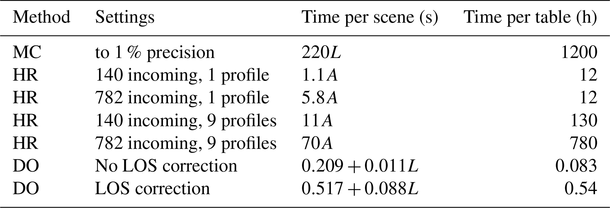
SASKTRAN-DO is going to be the fastest option for most applications, unless two- or three-dimensional analysis is required. Currently SASKTRAN-DO is only configured to multithread over wavelength, and these are single wavelength calculations, so the times will be improved further when multithreading over other parameters is implemented. Monte Carlo is clearly not suitable for full table generation; even a modest precision of 1 % would require on the order of 1200 h of computation. The time required for precision N is proportional to $N^{-\mathrm{1}/\mathrm{2}}$, so, for example, to achieve 0.5 % the computation time would increase by a factor of 4. SASKTRAN-HR AMFs will be sped up in the future when full linearization is implemented, removing the need for redundancy in the finite-difference approach.

5 SASKTRAN AMF tables

SASKTRAN-derived box-AMF profiles have been used by Griffin et al. (Griffin et al., 2019, 2021) from Environment and Climate Change Canada (ECCC) to analyze TROPOMI measurements over North America. The first application compared TROPOMI data with in situ aircraft, in situ ground-based, and remote ground-based NO₂ measurements over the Canadian oil sands, improving agreement through the use of regional retrieval inputs with higher resolutions. The second application examined NO₂ retrievals over North American forest fires from 2018 and 2019, this time improving agreement between TROPOMI and aircraft measurements in part by using box-AMF profiles that explicitly account for aerosol content.

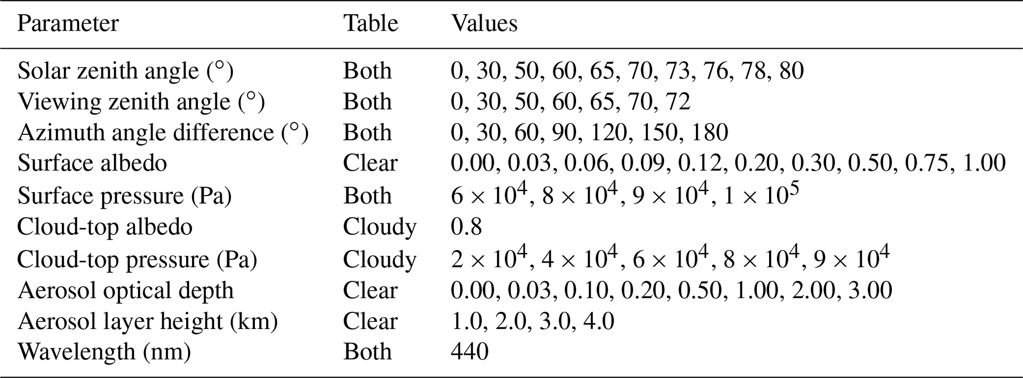
Table 3 outlines the parameter space for the AMF lookup tables. All tables were done on a 500 m vertical grid. The original table spanned 0 to 16 km at a wavelength of 440 nm for use with tropospheric NO₂. Subsequent tables added one or more of the following features: extending up to 50 km, adding another wavelength at 330 nm, and adding explicit aerosol layers. Aerosol layers are constant from the surface to 0.5 km below the layer height, then go linearly to zero at 0.5 km above the layer height. A refractive index of 1.5+0.1i at 440 nm and a lognormal particle size distribution with mode radius 0.1 µm and a width of σ=0.3 is assumed. Further modifications, such as ozone parameterizations, non-Lambertian surface reflection, or even parameterizations accounting for horizontal inhomogeneity, are certainly possible. SASKTRAN-HR was used for all of the tables up to this point, with nominal settings similar to those used for the middle panel of Fig. 2, which show agreement of about 1 % with SASKTRAN-MC; multiple diffuse profiles and high-density incoming grids were deemed unnecessary for the range of viewing geometries included in the tables. At the time the spherical corrections for SASKTRAN-DO were not implemented; now that they are available, future iterations can utilize this model.

Table 3 Parameters for SASKTRAN-HR AMF lookup tables used by ECCC. Aerosol optical depth and layer height were only used for the wildfire study (Griffin et al., 2021), not the oil sand study (Griffin et al., 2019).

6 Two-dimensional sensitivity study

In the following study, a potential application of SASKTRAN-HR's capacity for horizontally inhomogeneous atmospheres is demonstrated. A two-dimensional analysis is performed for a simplified TEMPO-like winter NO₂ measurement over the Canadian oil sands, a region of interest near the northern extent of the field of regard of TEMPO. A scenario with significant horizontal variation in both the NO₂ and the surface albedo is constructed; the total AMF is computed accounting for this variation and again while neglecting it. The difference quantifies the consequences of the assumption of horizontal homogeneity that one-dimensional analyses are built upon.

The scenario for this study was inspired by simulated and measured data in order to ensure realistic values but was greatly simplified in order to keep interpretation manageable. Two NO₂ profiles, one with surface pollution and one without, were selected from the scene shown in Fig. 8, taken from the global tropospheric chemistry simulations by Hu et al. (2018). The surface reflection is assumed to be Lambertian for simplicity, with an albedo of 0.8 in the south (approximating the reflectivity of snow) and 0.2 in the north. These values were selected as a rough representation of the Moderate Resolution Imaging Spectroradiometer (MODIS) data shown in Fig. 8, which is the nadir BRDF-adjusted reflectance (NBAR) from band 3 that spans 459 to 479 nm (Schaaf and Wang, 2015). Both scenes were taken from 15 December 2013 at 18:00 UTC. Pressure, temperature, air number density, and ozone number density are all horizontally homogeneous, with values taken from the US Standard Atmosphere (Dubin et al., 1976), and no aerosols were included.

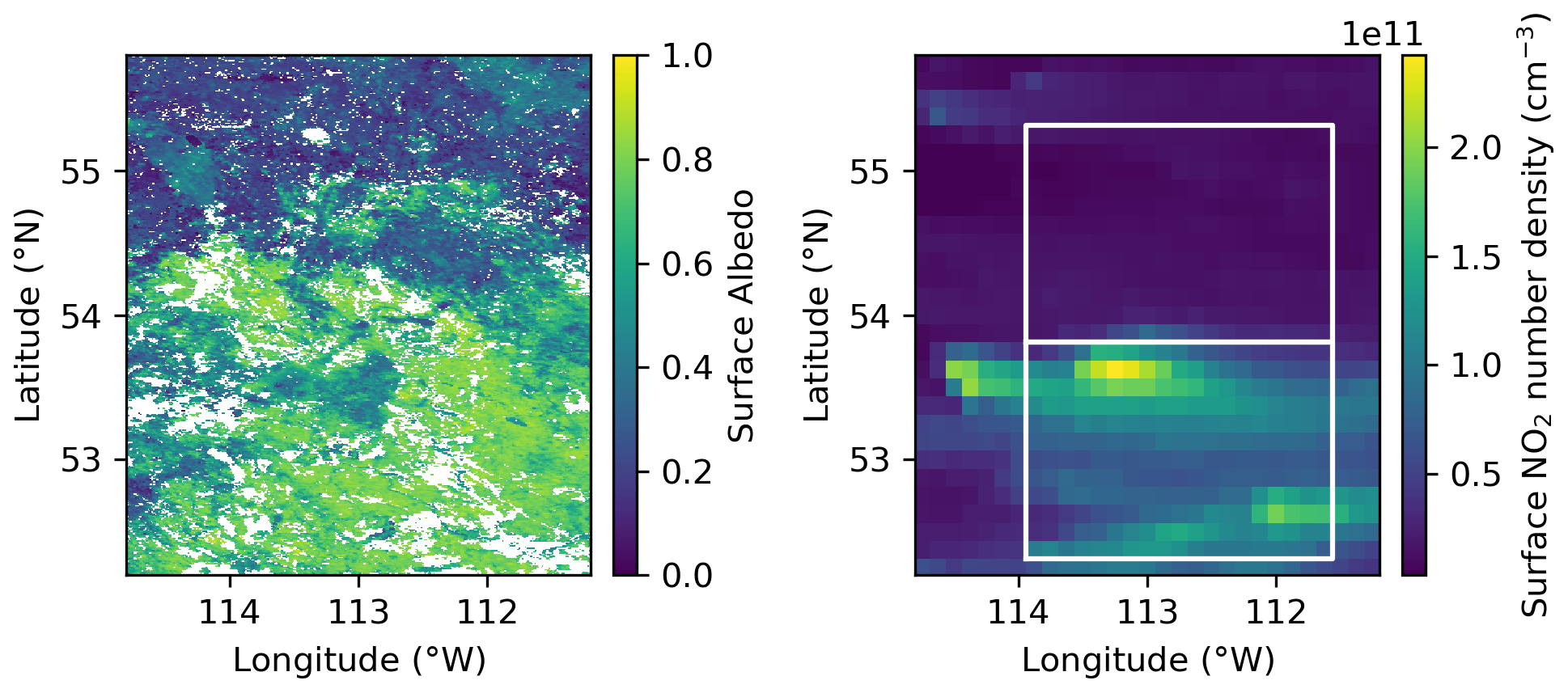
Figure 8 Surface albedo and surface NO₂ data used to justify the simplified scenario for the two-dimensional study. The albedo is the nadir BRDF-adjusted reflectance MODIS data (Schaaf and Wang, 2015) and the NO₂ is simulated (Hu et al., 2018). White patches in the surface albedo indicate missing data. The polluted NO₂ profile is the average of the profiles found in the southern white box, and the unpolluted profile is similarly from the northern box.

The simplified two-dimensional scenario is illustrated in Fig. 9, showing the polluted NO₂ profile over snow in the south and the unpolluted NO₂ profile over a surface with a lower albedo in the north. It also shows line of sight and the direct sun beam for the TEMPO-like viewing geometry on a winter day at approximately 54^∘ latitude, with a viewing zenith angle of 62^∘ and a solar zenith angle of 78^∘.

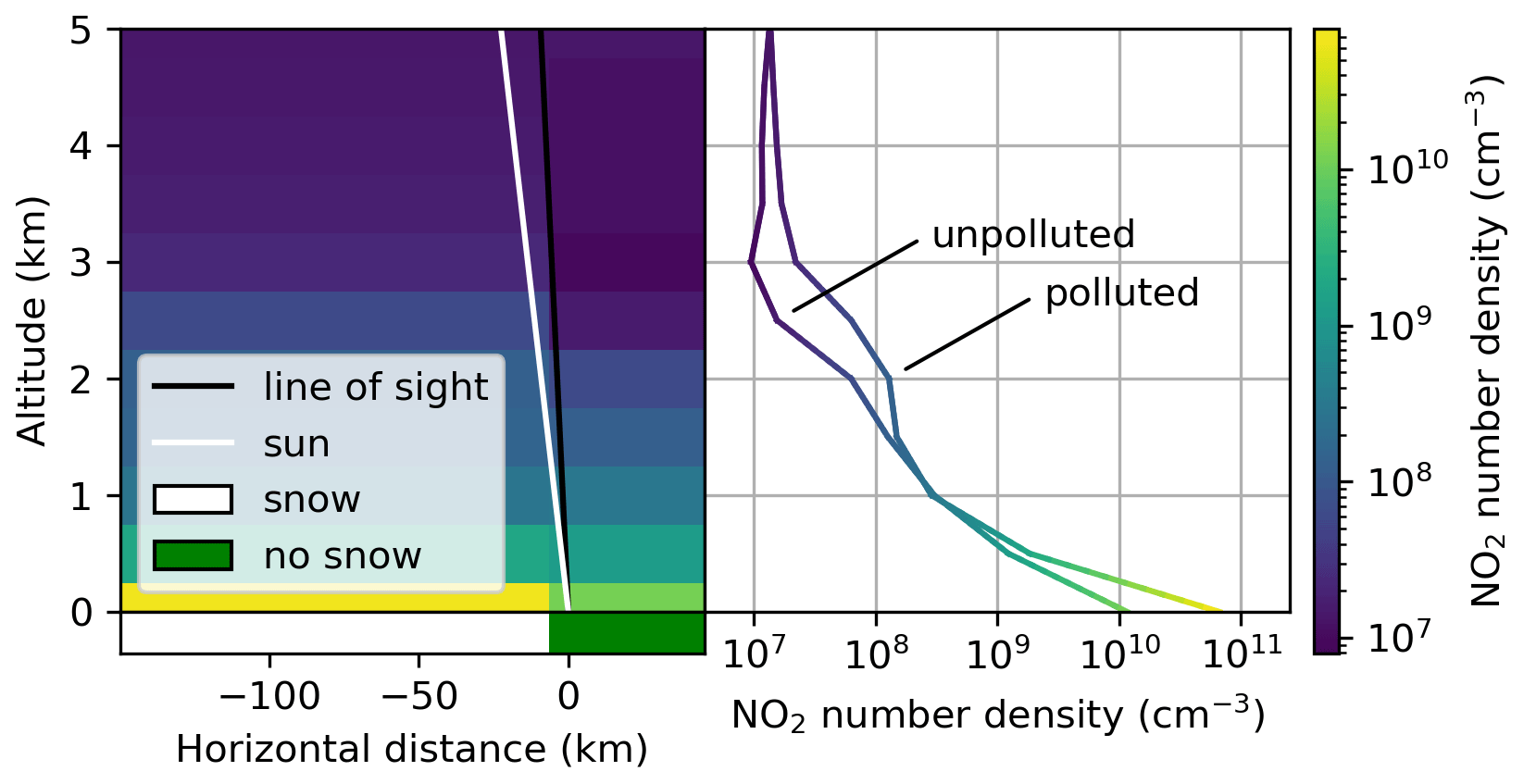
Figure 9 Scenario used for the two-dimensional sensitivity study. Shown is a TEMPO-like measurement of an unpolluted scene over a surface albedo of 0.2, but heavy pollution over snow (surface albedo 0.8) is found to the south.

The first step was to compute two-dimensional box-AMFs, with and without the horizontally varying surface albedo. The same box-AMFs were used for both the horizontally homogeneous and inhomogeneous NO₂ cases, as box-AMFs are insensitive to absorber profile. They were computed across approximately 200 km horizontally and up to 5 km in altitude, covering most of the sensitivity to horizontal variability for this scenario. The two-dimensional box-AMFs, along with their corresponding one-dimensional box-AMFs, are shown in Fig. 10. As expected, neglecting the high reflectivity to the south results in an underestimation of the box-AMFs and therefore an underestimation of the measurement sensitivity. Note that each column is the approximate width of four TEMPO pixels at this latitude.

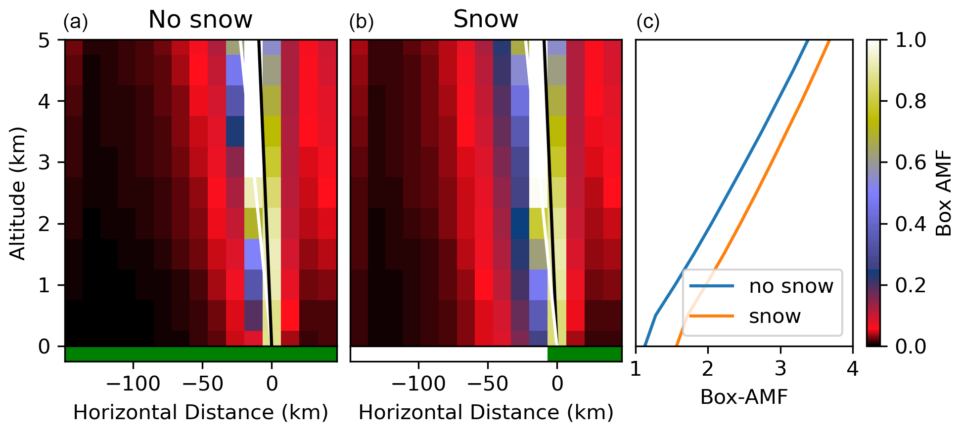
Figure 10 Two-dimensional box-AMFs with and without a region of high reflectivity south of the ground pixel. The outermost columns represent the contribution from the entire field beyond what is shown here; this is why these box-AMFs increase slightly while the trend is clearly decreasing. The sum of all two-dimensional box-AMFs at a given altitude recovers the traditional one-dimensional box-AMF, shown in (c).

The second step is to compute total AMFs by taking weighted averages of the box-AMF values using NO₂ concentrations as weights (see Eq. 32). Figure 11 shows the partial slant columns s_ij, which are an intermediate quantity in this computation. Note that the sum of all s_ij returns the total slant column so that Fig. 11 is a visualization of the distribution of the origin of the measured signal. The enhancement in signal originating from the lowest layers south of the ground pixel is evident, particularly when both the albedo and the NO₂ are increased in the bottom right panel.

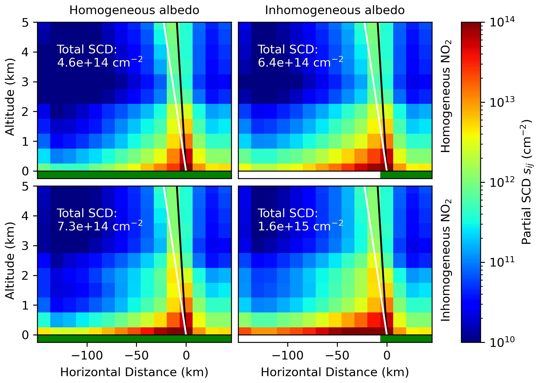
Figure 11 Partial SCD distribution for scenes with horizontally homogeneous and inhomogeneous surface albedo and NO₂. The sum of each pixel returns the total SCD that would be measured by the instrument.

First, consider the total AMF for a scenario with variable surface albedo as described in the original scenario, but with horizontally homogeneous NO₂. Combining the box-AMFs computed with uniform surface albedo with the horizontally homogeneous NO₂ (see Fig. 11, top left) results in an AMF of 1.21; this is what a one-dimensional analysis would return. Combining the box-AMFs computed with the variable surface albedo with the horizontally homogeneous NO₂ (see Fig. 11, bottom left) results in an AMF of 1.64. Neglecting the change in surface albedo for this scenario results in underestimating the total AMF by 26 %.

Second, consider a scenario with horizontally inhomogeneous NO₂ as described in the original scenario above, but with uniform surface albedo. The one-dimensional analysis of this scene is identical to the previous, resulting in a total AMF of 1.21. The two-dimensional analysis combines the uniform surface albedo box-AMFs with the true NO₂ field (see Fig. 11, top right), resulting in a total AMF of 1.91. Neglecting the horizontal change in NO₂ for this scenario results in underestimating the total AMF by 37 %.

Finally, in the same way, consider the original scenario with horizontal variation in both surface albedo and NO₂; here (see Fig. 11, bottom right) the true total AMF is 4.05, meaning that neglecting both horizontal changes together results in underestimating the total AMF by 70 %.

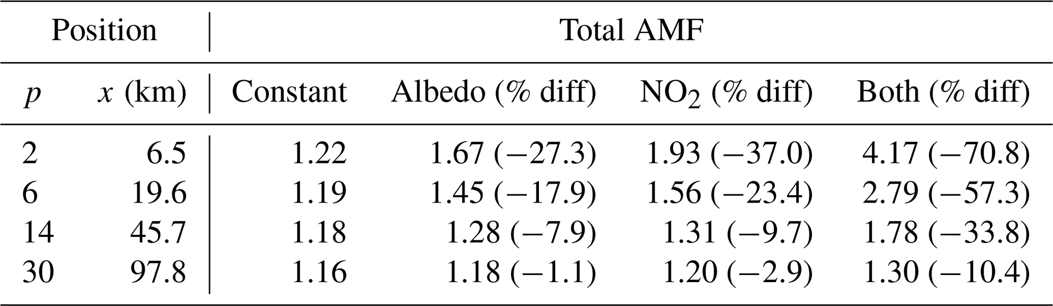
These results are somewhat severe due to the close proximity of the ground pixel to the sudden jump in surface albedo and NO₂; perhaps the more interesting question is how far away from such a feature the ground pixel needs to be before the effects become negligible. Table 4 summarizes the results of the same analysis while the ground pixel is moved progressively further north. With either feature on its own, errors on the order of 10 % can be found at a distance of nearly 50 km; with both features combined 10 % errors can be found at a distance of nearly 100 km.

Table 4 Effects of neglecting horizontal variation on total AMF. The distance of the ground pixel from the change in albedo$/$NO₂ is given in TEMPO pixels by p and in distance by x. The column headings for total AMFs indicate which quantity has horizontal variation in the simulated scene, and the percent difference quantifies the error when this variation is ignored when computing the AMF.

The usefulness of such a strategy for accounting for horizontal variations could be evaluated in an operational setting by comparing these errors with other sources of error. AMF errors are already quite high; for example, the typical errors of NO₂ AMFs for the Tropospheric Monitoring Instrument (TROPOMI) are estimated to be 15 % to 25 % but can easily exceed 50 % under the right circumstances (van Geffen et al., 2022). The above analysis suggests that horizontal variations could easily contribute errors on the order of 15 % to 25 %, but such occurrences are spatially sparse due to the requirement of large horizontal gradients. This analysis also does not account for the horizontal resolution of the input NO₂ field and albedo. The horizontal analysis of the radiative transfer implies a certain horizontal resolution to the measurement; if the input products match this resolution, such errors would be reduced.

This approach is not currently feasible on a large scale due to the large computational load, especially for the volume of data supplied by the normal operation of an instrument like TEMPO. Primary obstacles include high computation times required for two- or three-dimensional fields, difficulty in parameterizing such fields for a lookup table, and the accuracy and availability of prior trace gas fields at such high horizontal resolutions. Using this approach for smaller-scale studies or campaigns is much more feasible. For example, using it only for localized analysis of winter scenes containing select industrial or urban regions would filter out much of the data volume while maximizing occurrences of large horizontal gradients. It could also be used effectively for special observations from TEMPO that focus on events producing large gradients, such as forest fire observations with reduced revisit time (Zoogman et al., 2017).

Computation times could be greatly reduced by fully linearizing SASKTRAN-HR, which would eliminate redundancy in the current finite-difference approach; this upgrade is to be implemented within the next few years. Another potential improvement is separating contributions from the line of sight and single-scatter paths from the diffuse multi-scatter field, removing sharp features and permitting a large reduction in horizontal resolutions.

There are many potential alternative applications of a multidimensional AMF field to satellite measurements. For example, dependence on assumed NO₂ fields could potentially be reduced by analyzing multiple pixels simultaneously, utilizing the data from adjacent pixels which would otherwise be ignored. Such a method could be particularly effective for a localized analysis combining satellite measurements with in situ measurements. As another example, multidimensional AMF fields would add value as part of chemical data assimilation. Furthermore, they could be used to estimate an albedo and geometry dependent horizontal averaging kernel, characterizing the contribution of radiative transfer to the true horizontal resolution that is being measured.

7 Conclusions

SASKTRAN, originally designed for limb measurements, has been upgraded for use in nadir applications. Air mass factor computation has been added to the Monte Carlo method (SASKTRAN-MC), which serves as an important validation tool for the successive orders (SASKTRAN-HR) and discrete ordinates (SASKTRAN-DO) methods. SASKTRAN-DO has been equipped with spherical corrections which make the method feasible at extreme geometries. Air mass factors computed with all three methods were computed and found to be in good agreement. Agreement between SASKTRAN-HR and SASKTRAN-MC for moderate geometries was found to be on the order of 1 % with default settings and could be brought as low as 0.4 % by increasing the resolution of the downwelling and near-horizontal radiance field. Agreement on the order of 2 % can be achieved for extreme geometries, requiring the use of multiple diffuse profiles. Agreement between SASKTRAN-MC and SASKTRAN-DO (with spherical solar and line-of-sight corrections) was found to be on the order of 2 % for most geometries, with a distinct feature at mid-altitudes under all sun positions and viewing geometries due to the plane-parallel approximation in the multiple scattering.

SASKTRAN-HR is equipped to handle two- and three-dimensional features, providing a deterministic alternative to Monte Carlo for applications calling for horizontal analysis. For example, increased horizontal interference would be expected in the presence of strong horizontal gradients in surface albedo (e.g., light or variable snow, coastlines) or in trace gas concentrations (e.g., urban centers, industrial emitters, forest fires). SASKTRAN-HR was used to perform a sensitivity analysis on a simulated TEMPO scene over the Canadian oil sands, near the northern extent of its field of regard. The surface albedo was made to transition from 0.2 to 0.8 and the NO₂ field from unpolluted to polluted at varying distances from the ground pixel. The two-dimensional distribution of the light path and the measured NO₂ signal were calculated and visualized, and the impact of neglecting horizontal changes was investigated. Errors on the order of 10 % were estimated at distances up to 50 km with one of these features present and at distances up to 100 km with both.

This study demonstrates that error due to horizontal variability is significant for a TEMPO-like instrument in the presence of sufficiently large horizontal gradients in surface albedo or trace gas concentration. However, accounting for it on a large operational scale is not advised due to computational requirements and the sparsity of such gradients. Localized analysis of scenes that are expected to contain large gradients stand to benefit the most, such as winter scenes containing industrial or urban regions of interest or TEMPO special observations of events like forest fires. Future work includes increasing the computational efficiency of the multidimensional radiative transfer and exploring the effectiveness of nontraditional retrieval methods, such as simultaneous analysis for groups of adjacent pixels, explicit combination with other measurement sources, or injection into a climate–chemistry model.