INCHEM-Py v1.2: a community box model for indoor air chemistry

The Indoor CHEMical model in Python, INCHEM-Py, is an open-source and accessible box model for the simulation of the indoor atmosphere and is a refactor (rewrite of source code) and significant development of the INdoor Detailed Chemical Model (INDCM). INCHEM-Py creates and solves a system of coupled ordinary differential equations that include gas-phase chemistry, surface deposition, indoor–outdoor air change, indoor photolysis processes and gas-to-particle partitioning for three common terpenes. It is optimised for ease of installation and simple modification for inexperienced users, while also providing unfettered access to customise the physical and chemical processes for more advanced users. A detailed user manual is included with the model and updated with each version release. In this paper, INCHEM-Py v1.2 is introduced, and the modelled processes are described in detail, with benchmarking between simulated data and published experimental results presented, alongside discussion of the parameters and assumptions used. It is shown that INCHEM-Py achieves excellent agreement with measurements from an experimental campaign which investigate the effects of different surfaces on the concentrations of different indoor air pollutants. In addition, INCHEM-Py shows closer agreement to experimental data than INDCM. This is due to the increased functionality of INCHEM-Py to model additional processes, such as deposition-induced surface emissions. A comparative analysis with a similar zero-dimensional model, AtChem2, verifies the solution of the gas-phase chemistry. Published community use cases of INCHEM-Py are also presented to show the variety of applications for which this model is valuable to further our understanding of indoor air chemistry.

1 Introduction

In recent years, the quality of the air we breathe has gained increased attention. The World Health Organisation (WHO) recently stated that exposure to indoor and outdoor air pollution was one of the greatest risks to human health and that improving air quality was necessary to reduce the global incidence and impact of diseases such as lung cancer, stroke and asthma (World Health Organisation, 2001). Much of the focus in developed countries to date has been on outdoor air quality, particularly in relation to attaining regulatory guidelines. However, exposure to air pollution indoors is arguably more important, given we are estimated to spend around 90 % of our time indoors in high-income countries like the United Kingdom (Klepeis et al., 2001). Moreover, the recent COVID-19 pandemic has highlighted the importance of good indoor air quality, particularly around virus transmission.

Indoor air is a complex mixture of gas and particles, primarily as a result of numerous emission sources. These include activities such as cooking, cleaning, air freshener or scented candle use, household improvement activities (such as painting), emissions from building and furnishing materials (Uhde and Salthammer, 2007; Weschler, 2009), and emissions from building occupants through breathing and interactions with compounds from skin (Nazaroff and Weschler, 2004; Wisthaler and Weschler, 2010). Typical indoor pollutants include volatile organic compounds (VOCs), nitrogen oxides (NO_X) and particulate matter (PM). In addition, VOCs produced from indoor sources, or via ingress into buildings through windows, doors and cracks in the building fabric, can evolve over time through reactions with oxidant species, such as ozone (O₃) (Liu et al., 2021), hydroxyl radicals (OH) (Carslaw et al., 2017) and nitrate radicals (NO₃) (Arata et al., 2018). This secondary chemistry can result in the formation of a wide range of secondary products, such as formaldehyde and secondary organic aerosol (SOA), which can have a high potential for causing health issues, when compared to the parent VOC. For example, formaldehyde is a known carcinogen, and SOAs are associated with a range of cardiovascular and respiratory conditions (Schraufnagel, 2020; WHO Air quality and health Guidelines Review Committee, 2010). Given that long-term monitoring of such processes has been limited to date, indoor air chemistry models provide a useful tool to aid further understanding, particularly of the evolution of secondary chemistry over time.

In recent years, there have been significant advances in our understanding of indoor air quality. This is due, in part, to some larger-scale, intensive indoor measurement campaigns in test houses, involving a suite of advanced instrumentation more typically used in outdoor field campaigns (see the overview in Farmer et al., 2019). The results from these campaigns have demonstrated that indoor air quality is a complex, multidimensional problem, where indoor and outdoor sources, transformation processes, and building design, management and use are the driving physical and chemical factors for air quality. Human behaviour then adds further complexity. Ideally, one would perform numerous measurements in numerous buildings and for long periods of time to understand these processes. However, such a task would be expensive, time-consuming and logistically challenging. For instance, how would representative buildings be selected? An alternate approach is to simulate these processes in a model, coupled with evaluation using experimental data. It is then possible to use the evaluated model to provide forecasts and to explore hypothetical scenarios not possible through measurements, thus providing a deeper insight into the processes of interest.

There are numerous processes that need to be considered in a model of indoor air quality; these include direct and secondary emissions from surfaces (building materials, furnishings and people), physical building parameters (such as ventilation rates, temperature, humidity and light), gas- and particle-phase chemistry, surface deposition, and the effect of occupants. These factors will combine to determine the occupant exposure to air pollution under any set of building conditions. Note that microbial emissions also play a role in occupant exposure to indoor air pollution, but they have not been considered in this work.

The INdoor CHEMical Model in Python (INCHEM-Py) is a zero-dimensional community box model that includes many of these processes to enable investigation of the evolution of indoor air chemistry over time. It is a refactor (rewrite of source code) and improvement of the INdoor Detailed Chemical Model (INDCM) developed by Carslaw (2007) and is the most detailed chemical model that currently exists for exploring the chemistry of indoor atmospheres. It allows the user to understand the change in concentrations of indoor species over time and the key reaction pathways that describe the formation, transformation and loss of indoor species. Processes included within INCHEM-Py have been developed and implemented as our understanding of the indoor environment has improved, when experimental data have supported new developments, and according to the research questions being asked. The model is continuously being improved; this paper gives a snapshot of the current version of the model while also defining the foundation upon which future model developments will build upon. INCHEM-Py v1.1 has been described in basic detail, covering accessibility and broad function in Shaw and Carslaw (2021). This paper describes the model in more detail, including the developments included in the latest version (v1.2), and gives some examples of the ways in which it can be used by the scientific community.

2 Model description

INCHEM-Py creates and solves a series of first-order ordinary differential equations (ODEs), with each equation representing the rate of change of a species concentration ($\mathrm{molec}.{\mathrm{cm}}^{-\mathrm{3}}$) with time. The general equation for these ODEs is shown for the concentration (C) of species i in Eq. (1).

$$\begin{array}{}\text{(1)}& {\displaystyle \frac{\mathrm{d}{C}_{\mathrm{i}}}{\mathrm{d}t}}=\sum R_{ij}+({\mathit{\lambda }}_{\mathrm{r}}{C}_{\mathrm{i},\text{out}}-{\mathit{\lambda }}_{\mathrm{r}}{C}_{\mathrm{i}})-\sum {\mathit{\nu }}_{\mathrm{d}}\left({\displaystyle \frac{A}{V}}\right)C_{\mathrm{i}}\pm k_{\mathrm{t}}\end{array}$$

The chemical mechanisms are represented with the first term on the right-hand side of Eq. (1) as a sum of all reaction rates involving species i, with j representing other species. Each reaction between species takes place at a rate, R (s⁻¹), dependent on the concentrations of the reactant species and the rate constant. The second term of each ODE accounts for indoor–outdoor exchange, which depends on the air change rate, λ_r (s⁻¹), and the species concentrations both indoors (C_i, $\mathrm{molec}.{\mathrm{cm}}^{-\mathrm{3}}$) and outdoors (C_i,out, $\mathrm{molec}.{\mathrm{cm}}^{-\mathrm{3}}$). The third accounts for surface deposition, dependent on the species deposition velocity, ν_d (cm s⁻¹), and surface-to-volume ratio of multiple surfaces ($A/V$, cm⁻¹), while the final term is for timed emissions, where k_t (s⁻¹) is the emission/loss rate of species i at time t.

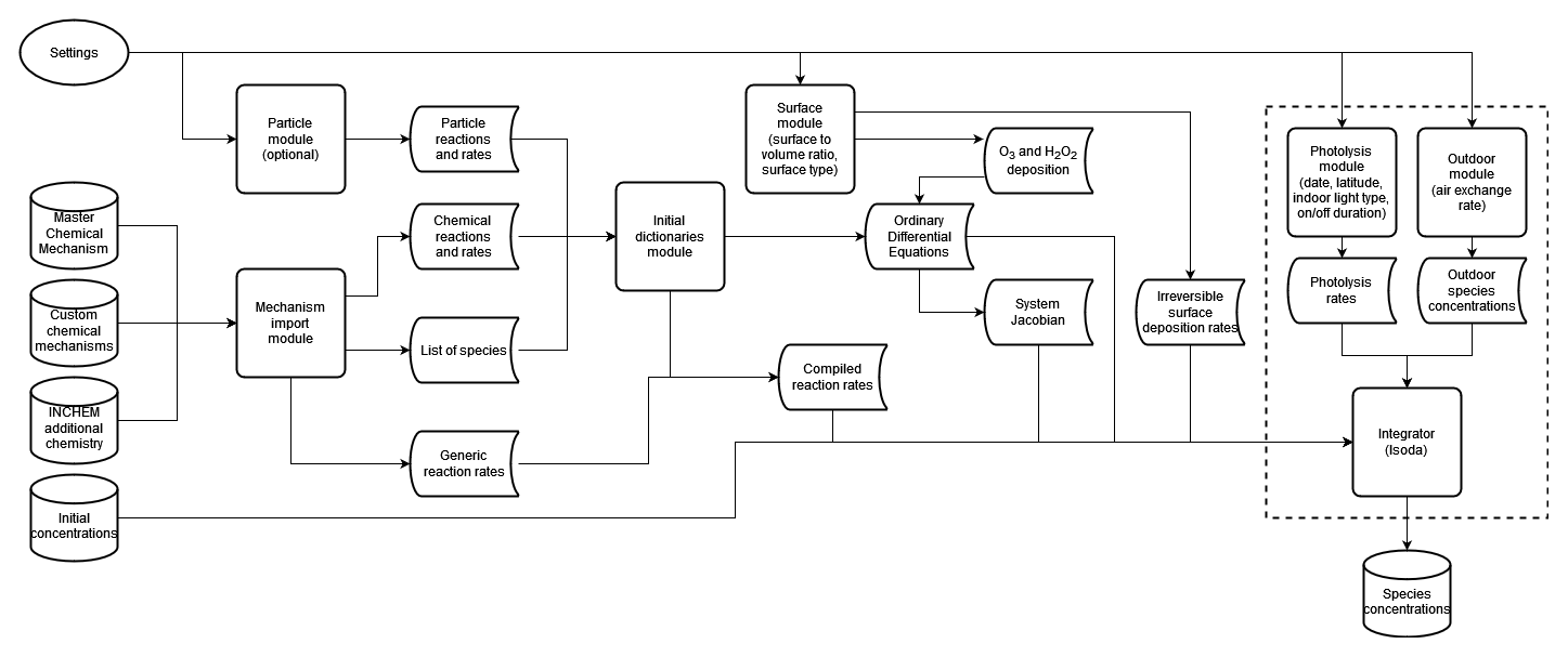
Figure 1 Flow chart showing the order of operations within INCHEM-Py. The modules and parameters within the dashed box are solved within the function that is passed to the integrator and are therefore called/calculated at every integrator internal time step.

Rate coefficients and reactions are imported for the most part from the Master Chemical Mechanism (MCM) (Jenkin et al., 1997, 2003, 2015, 2018, 2020; Saunders et al., 2003; Bloss et al., 2005), an almost explicit chemical mechanism following the atmospheric degradation of 135 VOCs. Additional schemes and mechanisms for species that are not included in the MCM, but which do occur indoors, are parsed from an additional file. Schemes have been developed for some terpenoids that are present in many scented items found and used indoors (Carslaw, 2007, 2013; Carslaw et al., 2012, 2017; Terry et al., 2014). Chlorine schemes have also been designed and implemented, since it is a key pollutant from bleach cleaning products (Wong et al., 2017). The full list of additional schemes is available in the user manual. The model also allows users to add their own chemical mechanisms to supplement those already included or to use a mechanism other than the MCM (although any new mechanisms need to be in the same format as that adopted in INCHEM-Py). Such flexibility will facilitate reaction mechanism development and community-driven model development.

All species within the model are assumed to egress with a specified air change rate (λ_r) as a function of their indoor concentration (C_i). Some species also ingress at the same air change rate, depending on their constant or diurnal outdoor concentrations (C_i,out) as discussed in Sect. 2.3. Species are also assumed to irreversibly deposit to surfaces at a rate dependent on individual deposition velocities (ν_d, mostly taken from Carslaw et al., 2012) and the surface-area-to-volume ratio (A/V) of the simulated space, as in Carslaw (2007). An optional mechanism for O₃ and H₂O₂ surface deposition and subsequent emission has been developed with a detailed discussion in Sect. 2.8. Additional emissions, both constant and intermittent, can be user defined. Gas-to-particle partitioning reactions are included for limonene, α-pinene and β-pinene (discussed in Sect. 2.4). The total size of the mechanism solved by INCHEM-Py (v1.2), before any additional user mechanisms are added, is 6507 chemical species and particles undergoing 19581 gas-phase reactions and gas-particle partitioning reactions. Figure 1 shows how input parameters are utilised within the modules of INCHEM-Py and how they produce the system of equations and parameters required to predict the evolution of indoor atmospheric constituents with time.

2.1 ODE formation and solution

All gas-phase reactions solved in INCHEM-Py are of the general form

$$\begin{array}{}\text{(2)}& C_{\mathrm{i}}+\mathrm{\dots }+C_j\stackrel{k}{=}{C}_x+\mathrm{\dots }+C_y,\end{array}$$

where C_i remains the concentration of an individual species and k is the rate constant of the reaction, which may be constant or depend on other variables such as photolysis. In each case, the concentration of species on the right-hand side of the equation is increased, and the species on the left-hand side (lhs) of the equation are decreased at the same rate (R) of

$$\begin{array}{}\text{(3)}& R_{ij}=\left(\prod C_{\text{lhs}}\right)k,\end{array}$$

where k is negative for the reactants and positive for the products. Therefore, by calculating ±R for each species in each reaction, the total change in an individual species concentration only through gas-phase reactions is given by the sum of all of the individual reaction rates, as follows:

$$\begin{array}{}\text{(4)}& {\displaystyle \frac{\mathrm{d}{C}_{\mathrm{i},\text{Gas}}}{\mathrm{d}t}}=\sum R_{ij}.\end{array}$$

Stoichiometries are dealt with in the MCM export by repeating the species within the reaction; i.e. the photolysis reaction H₂O₂ = 2OH is represented as H₂O₂ = OH + OH. This method is used throughout INCHEM-Py. Each species with the potential to partition to the particle phase has a corresponding term that tracks the change in its particle-phase concentration over time. This change in concentration for each partitioning species is determined by the equilibrium between the absorption to and desorption from the particle bulk based on its individual properties (Carslaw, 2007). Therefore, the particle-phase concentration of each species is represented by its own ODE in the system, and individual species contributions to total particle concentration can be output (particles are discussed in detail in Sect. 2.4).

The ODEs for each species are solved simultaneously using integrate.ode from the SciPy Python library and the wrapped LSODA function from the Fortran solver package ODEPACK (Hindmarsh, 1983). LSODA was chosen as the solution method as it automatically switches between the implicit Adams–Moulton formulae for non-stiff problems and backward differentiation formulae (BDF) for stiff problems. Due to the size of the system, and its highly coupled structure, the problem is stiff in most cases (note that if using only a small selection of the MCM mechanism it may be non-stiff in some instances). LSODA makes use of the Jacobian of the system to ease concentration predictions and is calculated in full as an array of partial differential equations by INCHEM-Py. The time step between outputs is set by the user in the settings file. The integrator will predict and output the solution to the ODE system at each time step. Default integrator parameters are given in the user manual and can be user adjusted. Verification of the solution of the gas-phase photochemistry is shown in Sect. 3.1.

2.2 Photolysis

Time is given in local solar time in INCHEM-Py and determined using the date and latitude of the simulation. A date input is used to calculate the solar declination angle (Dec) as

$$\begin{array}{}\text{(5)}& \mathrm{Dec}=-\mathrm{23.45}\times \cos \left({\displaystyle \frac{\mathrm{360}}{\mathrm{365.25}}}\times (d+\mathrm{10})\right),\end{array}$$

where d is the number of days since 1 January that year, −23.45 (^∘) is the solar declination angle at the winter solstice, 360 (^∘) is a complete angle, 365.25 is the number of days in the year, and 10 is the approximate number of days between the winter solstice and 1 January. Figure 2 shows the relationship between the declination and the solar zenith angle, θ, which is used to calculate the outdoor photolysis rates. In Fig. 2, CS represents a line connecting the centre of the Earth (C) with the centre of the Sun, Z represents the zenith of the location of the simulation, Lat is the latitude of the location of the simulation and LHA is the local hour angle which is 0 at solar noon. Using these known values and the spherical law of cosines the solar zenith angle is calculated as

$$\begin{array}{}\text{(6)}& \cos \left(\mathit{\theta }\right)=\sin \left(\mathrm{Lat}\right)\sin \left(\mathrm{Dec}\right)+\cos \left(\mathrm{Lat}\right)\cos \left(\mathrm{Dec}\right)\cos \left(\mathrm{LHA}\right).\end{array}$$

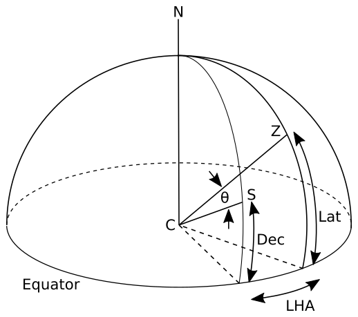
Figure 2 Relationship between declination angle (Dec), latitude (Lat) and solar zenith angle (θ). C is the centre of the Earth, the line CS is a line connecting the centre of the Earth to the centre of the Sun and Z represents the zenith of the location being simulated.

The solar zenith angle is used to calculate the solar photolysis portion of the overall photolysis rate (J), given by Eq. (7), for the 43 photolysis reaction rates currently included within the model. A description of the scattering method employed for this calculation is taken from Hayman (1997) and utilised in Saunders et al. (2003), where parameters l, m and n are optimised as per the discussion in Jenkin et al. (1997). These values are then attenuated according to the glass type chosen by the user through the use of a transmission factor (ψ). Indoor photolysis rate values (ϕ) are available for seven light types, and these are summed with the attenuated outdoor values to give the total photolysis rate as shown in Eq. (7).

$$\begin{array}{}\text{(7)}& J=\left(\right(l\cos \left(\mathit{\theta }{)}^m\exp \right(-n\sec \left(\mathit{\theta }\right)\left)\mathit{\psi }\right)+\mathit{\varphi }\end{array}$$

Values for ψ and ϕ are calculated and discussed in Wang et al. (2022). In brief, for the transmission factor, ψ, three typical glass types were selected from the analysis in Blocquet et al. (2018), covering a range of transmission values in both the UV (300–400 nm) and visible (400–800 nm) spectral ranges. The wavelength ranges were split into 10 nm intervals, and the percentage of light transmitted through each glass type and for each wavelength interval was defined. The absorption cross section and quantum yields for each photolysing species were used to calculate the weighted transmission factor, ψ, for each wavelength range as described in detail in Wang et al. (2022). The weighted transmission factor accounts for the proportion of the wavelength range transmitted by a particular glass type that is absorbed by each individual molecule. For the indoor photolysis rate, ϕ, the same wavelength ranges, intervals, quantum yields and cross sections were used, with spherically integrated photon fluxes from Kowal et al. (2017). Seven indoor light types are included in INCHEM-Py, covering a range of transmission spectra. The lights can be set to be on or off by the user for any period, over single or multiple days. Details of the specific lights simulated are found in Kowal et al. (2017); Wang et al. (2022).

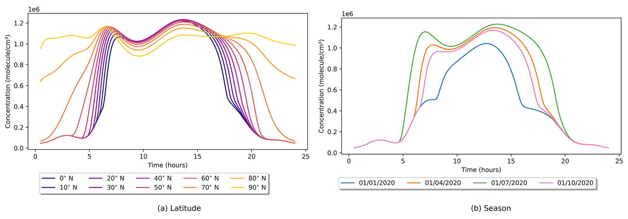
Figure 3 Indoor OH concentrations as a function of (a) latitude and (b) time of year. In both cases, only one setting is varied from default, with the latitude variation being on 21 June 2020 and the seasonal variation being at 45^∘ N. Note that 1 × 10⁶ $\mathrm{molec}.{\mathrm{cm}}^{-\mathrm{3}}$ is approximately 0.04 ppt.

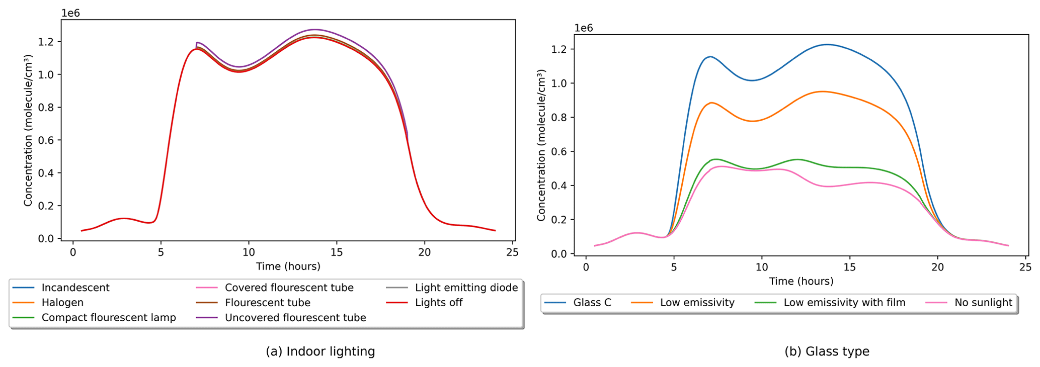
Figure 4 Indoor OH concentrations as a function of (a) indoor light source type and (b) glass type. All other values remained at their default settings.

The impact of the different photolysis parameters is shown in Figs. 3 and 4, where latitude and date settings are varied while all others remain at their default values. Figure 3a shows the effect of latitude variation in the Northern Hemisphere in summer on indoor OH concentrations. In moving away from the Equator, the length of the days increases, but the intensity of sunlight decreases. Therefore, this interplay results in peak indoor OH concentrations at midlatitudes. At the northern extremes, the Sun does not set; therefore, OH is produced through indoor photolysis reactions for the full 24 h period but at a reduced rate due to the lower intensity of solar radiation. Figure 3b shows the seasonal change of indoor OH in the Northern Hemisphere. Although the outdoor concentration of OH varies with latitude and season, its lifetime is too short for it to ingress indoors. OH production indoors is driven by the reaction of HO₂ with NO in this instance, so the OH profile indoors is driven by the NO concentration. Therefore, the tails of OH concentration in Fig. 3b follow the same minimum profile, only deviating with photolysis input. This minimum profile can be seen in Fig. 4b as the “No sunlight” trace.

Figure 4a shows the minimal impact of indoor lighting on the concentration of OH indoors, which contrasts with the large effects seen when the glass type is varied in Fig. 4b. The different glass types impact the production of OH indoors, mainly through the photolysis of HONO and the reaction of HO₂ and NO. Glass C lets through the most sunlight and, therefore, allows the most photolysis reactions to occur. At the other end of the scale is the low-emissivity glass with a reflective film that blocks out the majority of wavelengths and is very close to not having any sunlight enter the room at all. Without sunlight there is very little OH produced by the indoor lighting, which is set by default to come on at 07:00 LST (local solar time) and go off at 19:00.

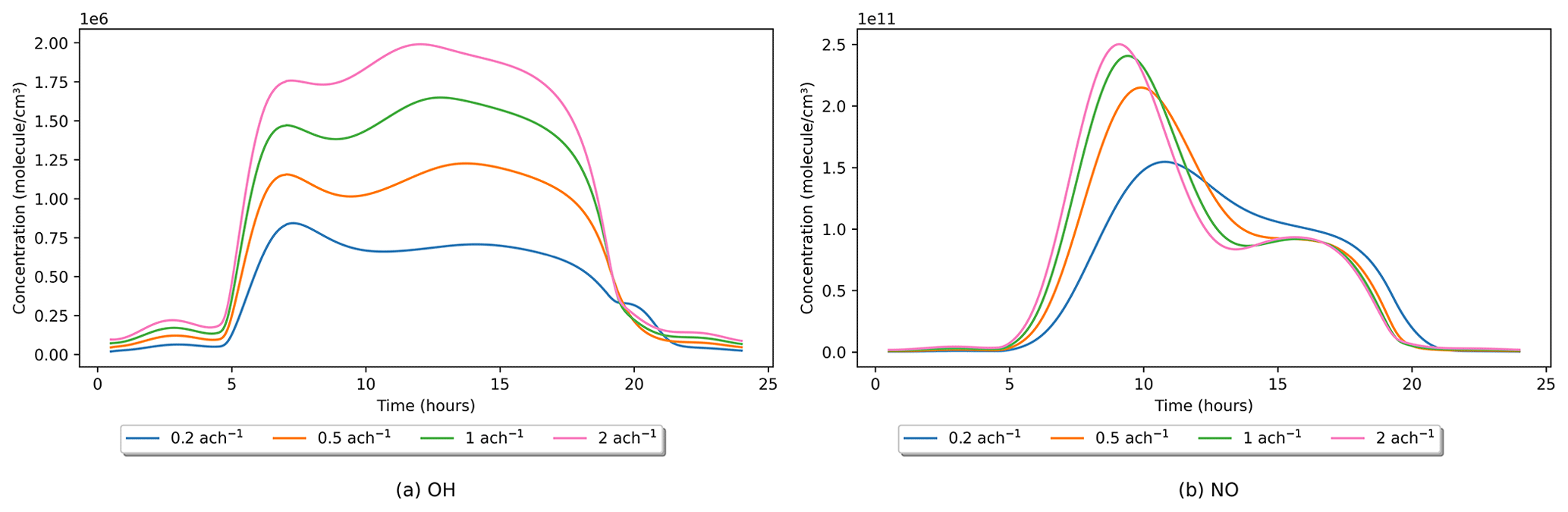
Figure 5 Indoor (a) OH and (b) NO concentrations as a function of air exchange rate. All other settings are the default values with the city outdoor concentration profile set to urban Bergen.

2.3 Outdoor air exchange

In INCHEM-Py only indoor species are predicted, and in some cases their concentrations will depend heavily on influx from and efflux to outdoors (Kruza et al., 2021). All indoor species are set to decay at a rate of λ_rC_i and to increase at a rate of λ_rC_i,out as in Eq. (1); however, only species for which measured, representative outdoor concentrations are available are assigned an outdoor concentration in the model. All other species (mostly short-lived intermediates) have outdoor concentrations set to zero.

Concentrations of OH, HO₂ and CH₃O₂ outdoors are photolysis driven and typically show strong diurnal variation outdoors. As in Carslaw (2007), the outdoor concentrations are set to peak at solar noon in the model, at 5 × 10⁶, 1 × 10⁸ and 2.5 × 10⁷ $\mathrm{molec}.{\mathrm{cm}}^{-\mathrm{3}}$, respectively, in line with measurements taken by Platt et al. (2002) and Emmerson et al. (2005). HONO shows the opposite trend, as it is photolysed during the day and is set to a minimum of ≈ 20 ppt at noon, peaking overnight at ≈ 300 ppt (Alicke, 2003).

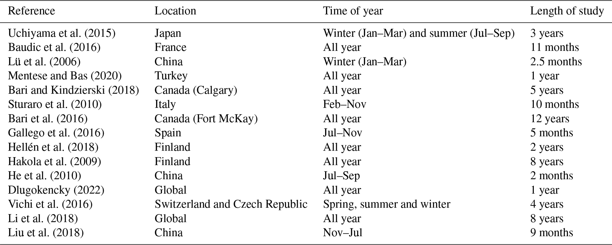
NO, NO₂ and O₃ have four possible diurnal profiles which can be chosen by the user, depending on their specific requirements. Profiles are provided for urban London (UK), suburban London (UK) and urban Bergen (Norway) locations, based on measured data from 2018 in the EEA (2018) air quality database. Details of these sites and their exact identifiers, including latitude and longitude, are given in the INCHEM-Py user manual. The data from each site were provided as hourly averages and in local time (UTC) by the meteorological station. Using the station longitude, each data point was shifted to solar time and quarter three (Q3) data were extracted. Q3 (July, August, September) was chosen because not all data sets had annual data for all species. The daily measurements were then overlaid, and an average data point for each hour was used to fit a trigonometric Fourier function for each location and species. The same process was used for outdoor concentrations of PM_2.5, which can also be included within the model when the particle module is enabled. The fourth location is Milan (Italy), which is included from Terry et al. (2014) as a particularly polluted 2-week period in August 2003. The measurements taken underwent the same procedure of averaging and fitting as the other three locations. The functions that have been input into the model are shown in the user manual. For INCHEM-Py v1.2 the constant outdoor concentrations have been updated, as shown in Table A1. These values have been sourced from published literature and measurement databases as referenced.

The outdoor concentrations used by INCHEM-Py can be adjusted to fit the requirements of the user. The default profiles of NO, NO₂ and O₃ from four European cities in the summer are provided as indicative locations with sufficient data to create the required diurnal profiles from the EEA (2018) air quality database. Further discussion on how the original profiles were created, how they may be adjusted and how to create additional profiles is provided in the user manual.

The rate of air change (ACR) is a user-defined variable that is input in units of acs⁻¹ (air changes per second) and will depend on how airtight the space being simulated is and any intentional ventilation. Weschler (2000) gives typical values of between 0.2 and 2 ach⁻¹ (air changes per hour) for tightly constructed and loosely constructed residential properties, respectively. The default value for INCHEM-Py is 1.38 × 10⁻⁴ acs⁻¹ (0.5 ach⁻¹). How the air change rate affects indoor OH concentrations (with all other values set to default) is shown in Fig. 5a.

Through the analysis of the reaction rates, as detailed in Sect. 2.7, OH is mainly produced through HO₂ + NO → OH + NO₂ and the photolysis reaction HONO → OH + NO, where HO₂ is the hydroperoxy radical that is primarily produced via the oxidation of VOCs. Most indoor NO comes from the photolysis reaction NO₂ → NO + O in the absence of indoor sources, and NO₂ is mainly produced by the reaction of NO + O₃ → NO₂. In general, increased ACR results in increased OH concentrations, but the lifetime of OH is too short to survive ingress through a building, and most OH indoors is made indoors through the above chemical reactions. The influx of outdoor OH is less than 0.009 % of the total production rate of OH at 0.5 ach⁻¹. NO, NO₂ and O₃ are also sourced from outdoors, so as the ACR increases, their concentrations increase, as do the rates of the reactions that produce higher OH as described above. Increasing ACR will also increase the loss rate of OH to outdoors; however, due to its reactivity this is less than 0.0025 % of the total loss rate of OH at 0.5 ach⁻¹.

In the 0.2 ach⁻¹ case, there is a small peak in OH concentration at 20:00 LST, which is not seen for the other ACRs. Analysing the reaction rates revealed that as ACR is reduced, indoor O₃ concentrations are reduced (as less is available to ingress from outdoors), which decreases the loss of NO through the reaction with O₃. This reduced NO consumption results in increased NO concentrations later in the day, as shown in Fig. 5b, compared to the higher-ACR cases. Increased NO concentrations increase the rate of the NO + HO₂ → OH + NO₂ reaction relative to the other simulations, therefore causing the peak in OH concentrations later in the day in the low-ACR case.

2.4 Particles

INCHEM-Py includes gas-to-particle partitioning for the oxidation schemes of limonene, α-pinene and β-pinene, producing 610 species that partition between the gas and aerosol phases. Carslaw et al. (2012) provides a full description of the method used to calculate the particle partitioning parameters, which is based on absorptive partitioning from Pankow (1994), whereby the phase of the species is determined by thermodynamic equilibrium. We assume that the particles are all in the PM_2.5 range and focus only on chemical composition, with no representation of how these particles evolve dynamically over time.

The method relies on a balance between the rate of VOC absorption to (k_on) and the rate of desorption from (k_off) particles. The partitioning constant, K_p (m³ µg⁻¹), is calculated for each species that partitions to the particle phase as

$$\begin{array}{}\text{(8)}& K_{\mathrm{p}}={\displaystyle \frac{\mathrm{7.501}RT}{W_{\text{om}}{\mathrm{10}}^{\mathrm{9}}{P}_{\mathrm{l}}}},\end{array}$$

where R is the ideal gas constant ($\mathrm{J}{\mathrm{K}}^{-\mathrm{1}}{\mathrm{mol}}^{-\mathrm{1}}$), T is the temperature (K), W_om is the mean molecular weight of the particle (g mol⁻¹) and P_l is the liquid vapour pressure of the species (Torr) (Pankow, 1994; Carslaw et al., 2012). k_on is set at a temperature-independent value of 6.2 × 10⁻³ ${\mathrm{m}}^{\mathrm{3}}\mathrm{\mu }{\mathrm{g}}^{-\mathrm{1}}{\mathrm{s}}^{-\mathrm{1}}$, which is based on Jenkin (2004) and Johnson et al. (2006). W_om is set to 120 g mol⁻¹ initially but is calculated for each subsequent integration step based on the composition of the formed particles. Assuming equilibrium conditions exist (Leungsakul et al., 2005), Eq. (9) allows the determination of k_off for each species.

$$\begin{array}{}\text{(9)}& K_{\mathrm{p}}={\displaystyle \frac{k_{\text{on}}}{k_{\text{off}}}}\end{array}$$

The rates k_on and k_off are used to track each species partitioning to and from the particle phase and are solved in the ODE alongside the gas-phase reactions. Each species is tracked individually in the particle phase and summed to produce a total number (tsp, $\mathrm{molec}.{\mathrm{cm}}^{-\mathrm{3}}$) and concentration (tspx, µg m⁻³) of suspended particles.

This method assumes particles already exist within the model for the initial absorption reactions to take place. A small number of seed particles are present within the model, set within the initial conditions file as “seed”. These seed particles do not change their number density but allow for partitioning to take place. Particles can also enter from outdoors with the outdoor particles assumed to be 30 % organic and 70 % inorganic. The organic fraction from outdoors is then also used as a seed on which new indoor particles can form. Particles are set to irreversibly deposit onto surfaces at a rate of 0.004 cm s⁻¹ (Sarwar and Corsi, 2007).

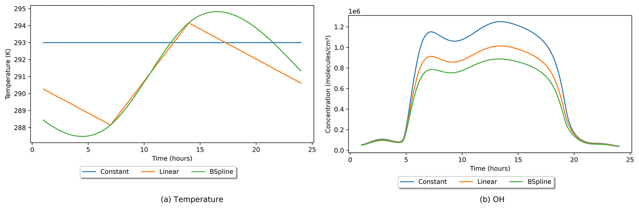
Figure 6 Results of the three different temperature input methods on (a) temperature and (b) OH concentration. Only the “spline” variable was adjusted from default values; the constant temperature method and value is the default option.

2.5 Temperature

Most chemical reactions in INCHEM-Py have a temperature dependence. Indoor temperatures in most scenarios will have minimal variation but in some cases might vary throughout a day. The model allows for three methods of setting the indoor temperature: a constant value, a linear interpolation between given temperatures, or a zero-degree B-spline interpolation between given temperatures. For both interpolation methods, a minimum of two temperatures at two distinct times must be given. INCHEM-Py compares the given times to the length of the simulation and duplicates points before and after the simulated period, if required. This ensures that there is an interpolated or given temperature value at all time points. Full details of the methods used are given in the INCHEM-Py user manual. Three different temperature profiles using the three different methods are shown in Fig. 6, alongside their impact on the OH concentrations. Both interpolated methods used the same times and temperature inputs.

Temperature is a variable that changes the rate coefficients of many of the reactions in INCHEM-Py: some will increase with temperature, while others will decrease. Although the three temperature profiles are in good agreement around the middle of the day, there is a large difference earlier on given how the three methods work. This difference in methods leads to different concentrations for some of the precursors for OH, allowing them to have a differential impact on OH chemistry later, depending on their lifetimes. The combination of the varying reaction rates and resultant concentrations produces the final profile in Fig. 6b.

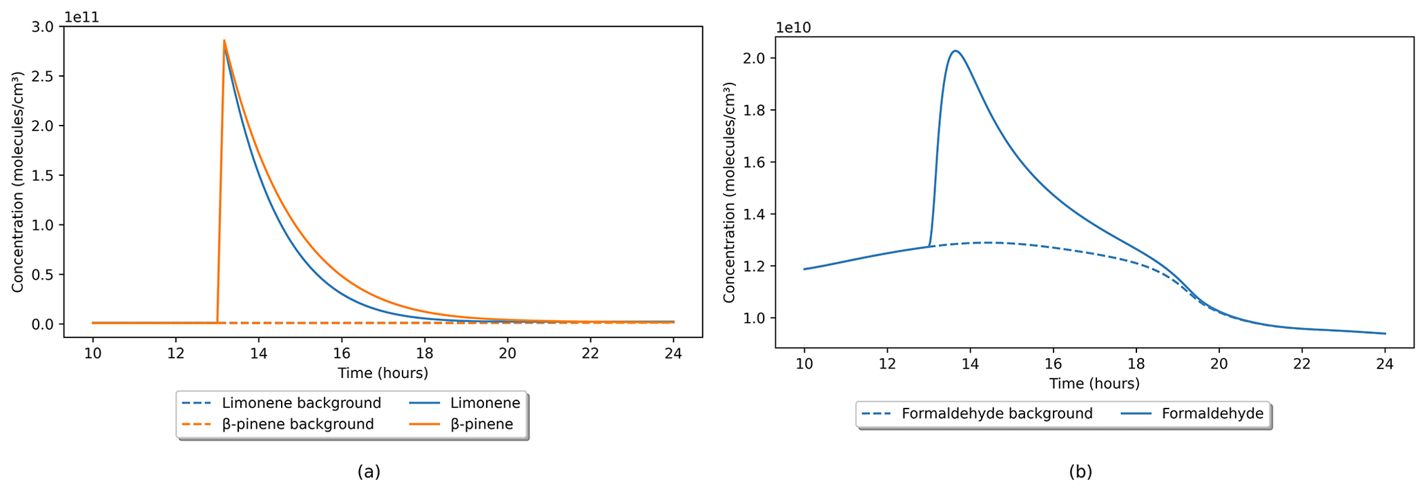
Figure 7 (a) Limonene and β-pinene timed emissions as a simulated cleaning event with (b) formaldehyde secondary emission compared to background default values.

2.6 Timed emissions

Term four in Eq. (1) accounts for user-defined timed emissions that can be input to simulate a release of a chemical species over a specific period of time. Only species that are solved by the model can be input; these include gas and particle species. Outdoor species cannot be input this way, as outdoor concentrations are not solved, but instead are input as time-dependent functions or constants which can be adjusted in the outdoor concentrations file. An example of this function is shown in Fig. 7, where an emission of limonene and β-pinene simulates the use of a cleaning product. Both species were input at a rate of 5 × 10⁸ $\mathrm{molec}.{\mathrm{cm}}^{-\mathrm{3}}{\mathrm{s}}^{-\mathrm{1}}$ (0.02 ppb s⁻¹) for 10 min at 1 pm, while all other settings remained at their default values. Figure 7a shows that, the terpene concentrations increase at the same rate and peak at very similar values. The small differences in the subsequent terpene decays are due to their different reactivities. For example, the reaction rate coefficients at 293 K for limonene with O₃ ($k_{{\mathrm{O}}_{\mathrm{3}}}$ = 2.0 × 10⁻¹⁶ ${\mathrm{cm}}^{\mathrm{3}}\mathrm{molec}{.}^{-\mathrm{1}}{\mathrm{s}}^{-\mathrm{1}}$) and OH (k_OH = 1.7 × 10⁻¹⁰ ${\mathrm{cm}}^{\mathrm{3}}\mathrm{molec}{.}^{-\mathrm{1}}{\mathrm{s}}^{-\mathrm{1}}$) are higher than for β-pinene ($k_{{\mathrm{O}}_{\mathrm{3}}}$ = 1.8 × 10⁻¹⁷ ${\mathrm{cm}}^{\mathrm{3}}\mathrm{molec}{.}^{-\mathrm{1}}{\mathrm{s}}^{-\mathrm{1}}$, k_OH = 8.1 × 10⁻¹¹ ${\mathrm{cm}}^{\mathrm{3}}\mathrm{molec}{.}^{-\mathrm{1}}{\mathrm{s}}^{-\mathrm{1}}$) (Jenkin et al., 2018). This explains the lower peak concentration and the faster decay for limonene, compared to β-pinene.

Figure 7b shows the secondary production of formaldehyde following the timed emission of limonene and β-pinene, compared with a background default value with no emissions. Using this method, we can simulate events where multiple chemical species interact to inform what proportions of an experimentally measured chemical are produced by primary emission or via secondary chemistry.

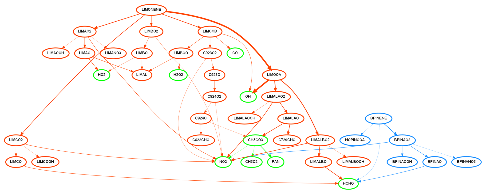
Figure 8 A flow chart showing the degradation pathways of limonene (orange) and β-pinene (blue) to final secondary products of interest (green). The fastest 95 % of reactions occurring at the time point where their concentrations are highest in Fig. 7 are shown. The thickness of the line is proportional to the absolute reaction rate, where the thicker the line, the faster the reaction. Nodes show species created, and all species are labelled in MCM format.

2.7 Reaction rate outputs

When analysing chemical transformations it is useful to know the rate at which a species is being produced or lost, as well as the relative importance of the individual reactions that are contributing to that rate. INCHEM-Py has an option to output the rates of all reactions at all time points. Using the rate coefficients and the calculated species concentrations, the reaction rates of individual reactions can be calculated at any time point in the simulation using Eq. (3). This function was developed for and used by Lakey et al. (2021) to identify important reactions and develop a reduced chemical mechanism for use in an indoor 3D fluid model.

In the case of the cleaning event shown in Fig. 7, the reaction rates from INCHEM-Py at each time step can be used to track the pathways linking the primary pollutants (limonene and β-pinene) to the secondary production of formaldehyde. This is visualised in Fig. 8, where a snapshot of the reaction pathways at the peak of the pollutant concentrations is shown. This method was used to analyse the contribution of surface cleaner formulations to indoor pollutants in Carslaw and Shaw (2022).

2.8 Surface deposition

Surface deposition of gas-phase species is an important aspect of indoor air chemistry, and the inclusion of surface deposition in indoor air models is key. Chemical species can be emitted from surfaces either as primary emissions or as secondary pollutants formed from gas-phase transformations which occur at the surface level. O₃ can deposit onto a range of surfaces and induce oxidation, releasing secondary pollutants as surface emissions (Gall et al., 2013; Cros et al., 2012). The rate of deposition to surfaces is surface-specific and is determined by mass transportation to the surface of a pollutant, as well as the uptake potential of the pollutant onto that specific surface (Reiss et al., 1994). The deposition rate of an oxidant onto a surface is also influenced by the air change rate, the bulk indoor concentration of the oxidant and the surface-to-volume ratios in the indoor environment (Coleman et al., 2008).

INCHEM-Py v1.1 simulates the irreversible deposition of 3371 indoor gas-phase species. However, it does not incorporate the secondary pollutants emitted from the surface. It also does not consider different surface materials and only calculates surface deposition based on estimated deposition velocities and a total-surface-to-volume ratio (Carslaw, 2007). These are retained in v1.2 alongside a new surface deposition mechanism onto multiple surfaces that has been developed for INCHEM-Py v1.2, based on the work of Kruza et al. (2017) and considering the rates of deposition and secondary pollutant emissions following individual O₃ and H₂O₂ deposition (Carter et al., 2023). Given that the nature of such interactions is likely to be complex and currently not fully understood, we consider the process occurs in two steps: deposition to the surface and loss of the oxidant, followed by emission of new species from that surface. The surface removal rate of O₃ and H₂O₂ in the model is determined by Eqs. (10) and (11), respectively:

$$\begin{array}{}\text{(10)}& {\displaystyle }{F}_{{\mathrm{O}}_{\mathrm{3}}}={\mathit{\nu }}_{{\mathrm{d}}_{{\mathrm{O}}_{\mathrm{3}}}}{\displaystyle \frac{A}{V}},\text{(11)}& {\displaystyle }{F}_{{\mathrm{H}}_{\mathrm{2}}{\mathrm{O}}_{\mathrm{2}}}={\mathit{\nu }}_{d_{{\mathrm{H}}_{\mathrm{2}}{\mathrm{O}}_{\mathrm{2}}}}{\displaystyle \frac{A}{V}},\end{array}$$

where $F_{{\mathrm{O}}_{\mathrm{3}}}$ and $F_{{\mathrm{H}}_{\mathrm{2}}{\mathrm{O}}_{\mathrm{2}}}$ represent the deposition rates (s⁻¹) of O₃ and H₂O₂ onto a surface, respectively. ν_d represents the surface deposition velocity of an oxidant in centimetres per second (cm s⁻¹), A is the surface area of an indoor surface or material in square centimetres (cm²), and V is the total volume of the indoor environment in cubic centimetres (cm³).

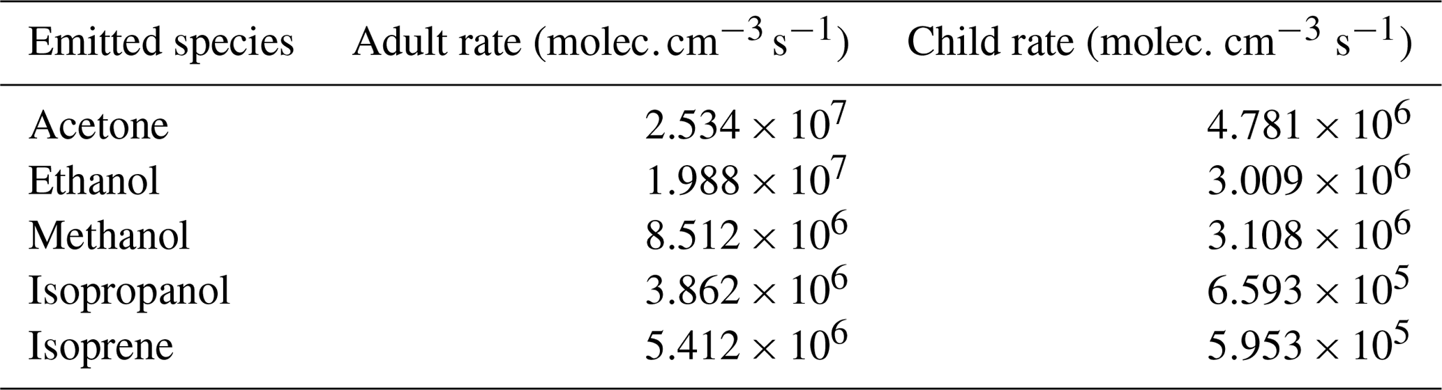
Table 1 Rates of breath and skin emissions for adults and children.

The emission rate calculations of secondary pollutants emitted as a result of oxidant surface deposition has been adapted from studies conducted by Morrison and Nazaroff (2002) and Kruza et al. (2017). The emission rates can be determined by solving Eqs. (12) and (13):

$$\begin{array}{}\text{(12)}& {\displaystyle }{E}_{\mathrm{i}}={\displaystyle \frac{A{\mathit{\nu }}_{{\mathrm{d}}_{{\mathrm{O}}_{\mathrm{3}}}}{Y}_{\mathrm{i}}{C}_{{\mathrm{O}}_{\mathrm{3}}}}{V}},\text{(13)}& {\displaystyle }{E}_{\mathrm{i}}={\displaystyle \frac{A{\mathit{\nu }}_{d_{{\mathrm{H}}_{\mathrm{2}}{\mathrm{O}}_{\mathrm{2}}}}{Y}_{\mathrm{i}}{C}_{{\mathrm{H}}_{\mathrm{2}}{\mathrm{O}}_{\mathrm{2}}}}{V}},\end{array}$$

where E_i represents the emission of secondary pollutants from a surface ($\mathrm{molec}.{\mathrm{cm}}^{-\mathrm{3}}{\mathrm{s}}^{-\mathrm{1}}$). Y is the production yield of gas-phase species following deposition (dimensionless), and $C_{{\mathrm{O}}_{\mathrm{3}}}$ and $C_{{\mathrm{H}}_{\mathrm{2}}{\mathrm{O}}_{\mathrm{2}}}$ represent the bulk concentrations of indoor O₃ and H₂O₂, respectively ($\mathrm{molec}.{\mathrm{cm}}^{-\mathrm{3}}$).

Surfaces included in the O₃ and H₂O₂ surface deposition mechanisms for INCHEM-Py v1.2 are soft fabric, painted, human skin, wood, metal, concrete, paper, plastic and glass. However, there are no data for H₂O₂ onto plastic, glass and skin surfaces. The mechanisms were constructed using surface-specific deposition velocities of O₃ and H₂O₂ and respective production yields from a range of experimental literature (Sabersky et al., 1973; Lin and Hsu, 2015; Klenø et al., 2001; Grøntoft, 2002; Abbass et al., 2017; Gall et al., 2013; Tamás et al., 2006; Cros et al., 2012; Coleman et al., 2008; Ye et al., 2020; Lamble et al., 2011; Rim et al., 2016; Poppendieck et al., 2007; Wang and Morrison, 2010, 2006; Nicolas et al., 2007; Morrison and Nazaroff, 2000; Fadeyi et al., 2013; Yao et al., 2020; Di et al., 2017; Rai et al., 2014; Fischer et al., 2013; Wisthaler and Weschler, 2010; Schripp et al., 2012; Mueller et al., 1973; Cox and Penkett, 1972; Grøntoft and Raychaudhuri, 2004; Simmons and Colbeck, 1990; Cano-Ruiz et al., 1993; Poppendieck et al., 2021). These mechanisms ensure secondary species, primarily aldehydes, are emitted from specific surfaces as a result of oxidant deposition. A deposition velocity taken from Carslaw (2007) has been added for plastic, glass and skin surfaces to account for gas-phase deposition of H₂O₂. Deposition of H₂O₂ onto these three surfaces does not produce any aldehyde emissions in our model.

A detailed description of the oxidant surface deposition mechanisms is found in a corresponding study conducted by Carter et al. (2023). Using these methods, further deposition mechanisms can be developed for other species and surfaces in the future, as relevant experimental data become available.

Since the Carter et al. (2023) study, the deposition module for INCHEM-Py has been updated to include O₃ deposition onto linoleum surfaces, using data from Kruza et al. (2017). The deposition velocity of O₃ onto plastic surfaces has also been updated as a result of an ongoing review of the literature. The deposition velocities of O₃ onto linoleum and plastic surfaces are now 0.0070 and 0.1225 cm s⁻¹, respectively (Coleman et al., 2008; Kruza et al., 2017; Klenø et al., 2001; Poppendieck et al., 2007; Nicolas et al., 2007; Wang and Morrison, 2006).

2.9 Direct emissions

Breath emission values from humans are optionally included in the model, according to occupancy status (Kruza and Carslaw, 2019; Weschler et al., 2007). The number of adults and children can be specified in the settings file, and a calculated emission in molecules per cubic centimetre per second ($\mathrm{molec}.{\mathrm{cm}}^{-\mathrm{3}}{\mathrm{s}}^{-\mathrm{1}}$) is used, as shown in Table 1. These emissions are constant for the duration of the simulation.

3 Model output and evaluation

In this section, the INCHEM-Py model is used to simulate previously published results from both experimental and modelling efforts. Settings and outputs from all of the model runs are linked in the data availability section of this paper.

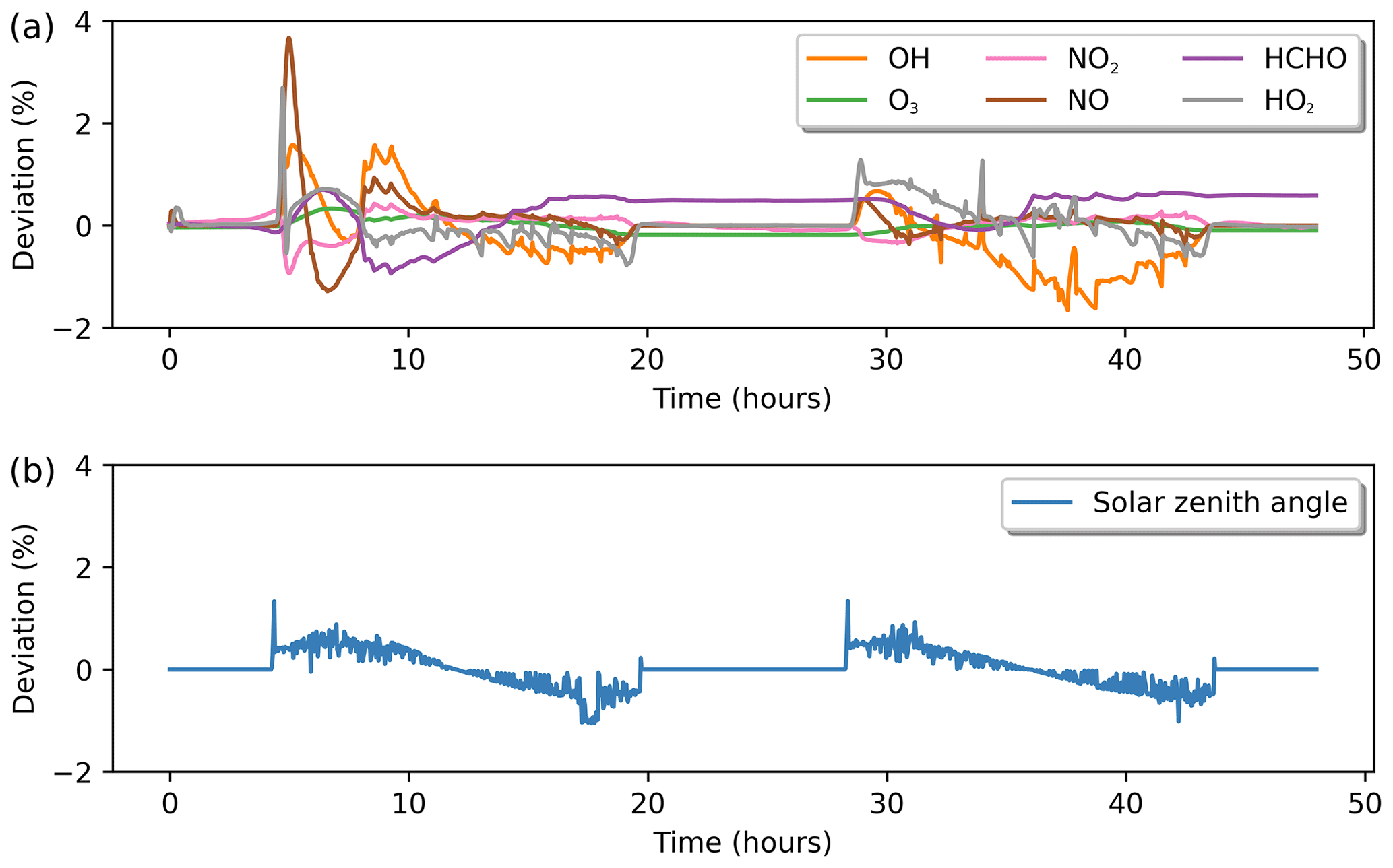
Figure 9 (a) Percentage deviation in gas-phase chemistry solutions between INCHEM-Py and AtChem2. Species are named as in the MCM. (b) The percentage deviation between the solar zenith angles as calculated by INCHEM-Py and AtChem2. Percentage deviation calculated by Eq. (14).

3.1 Gas-phase verification

The gas-phase photochemistry of INCHEM-Py is mainly constructed from the MCM, as discussed in Sect. 2. To validate the solution of this core component of the model, INCHEM-Py was set up to compare with AtChem2 (Sommariva et al., 2020). AtChem2 is an outdoor model that also utilises the MCM. INCHEM-Py was set up by disabling the features that are not easily reproducible in AtChem2, including the additional chemistry developed specifically for INCHEM-Py, particle processes, air change, indoor lighting and attenuation of outdoor light, and surface deposition and emission. A simulation was prepared in each model of a 2 d period representing 21 June 2020 at 45^∘ N, with no additional emissions. The percentage deviation (σ_i,t) for i at time t between the two models was calculated by Eq. (14), taken from O'Meara et al. (2020), where it was similarly used to validate gas-phase chemistry between AtChem2 and PyCHAM (a similar chamber focussed model).

$$\begin{array}{}\text{(14)}& {\mathit{\sigma }}_{i,t}=\left({\displaystyle \frac{s_{i,t}-b_{i,t}}{v\left(b_i\right)}}\right)\mathrm{100}\end{array}$$

In Eq. (14) the INCHEM-Py result is represented by s and the AtChem2 result represented by b. v(b_i) is the maximum value of component i and scales the difference between models to the individual component being compared.

Figure 9a shows the calculated differences for key species. INCHEM-Py performs well when compared to AtChem2, with the largest differences being during rapid increases or decreases in species concentration. The deviation is due to the calculation of photolysis parameters in Python-based INCHEM-Py vs. the calculations in Fortran-based AtChem. Values for Dec, cos (Lat)cos (Dec) and sin (Lat)sin (Dec) are identical to the thousandth between the two simulations propagating a small difference in the calculation of cos (θ) in Eq. (6). The larger deviation is due to the horizon placed within each model; a negative value for cos (θ) indicates that the Sun is below the horizon. AtChem2 limits the minimum value for cos (θ) to 0.01, whereas INCHEM-Py has a limit of 0. This means that the Sun begins to rise between 8 and 10 min earlier in INCHEM-Py, allowing photolysis reactions to begin to occur earlier and go on later. As shown in Fig. 9b, the value for solar noon shows no deviation.

3.2 H₂O₂ emission and fate

Zhou et al. (2020) studied the impact of non-bleach cleaning events in a combined chamber and modelling study. In this study, the INDCM model was used to explore secondary pollutant formation and the impact of different lighting levels on their concentrations. The INDCM had less complete representations of surface interactions, indoor photolysis and indoor–outdoor exchange. The original work was completed in parts per billion (ppb), and so outputs from INCHEM-Py have been converted for the comparison.

The indoor environmental quality chamber at the Building Energy and Environmental Systems Laboratory at Syracuse University had a mock residential room built within it. This 29.1 m³ room had a wooden frame, painted walls and a vinyl floor with no furniture present. Within this chamber a non-bleach H₂O₂ cleaning spray was used on a 0.75 m² area (12 squirts, 15 mL total) and then wiped dry over a period of 1–2 min. The surface-to-volume ratio of the experiment simulated here is 2 m⁻¹, and the floor is assumed to be one-sixth of the total surface area.

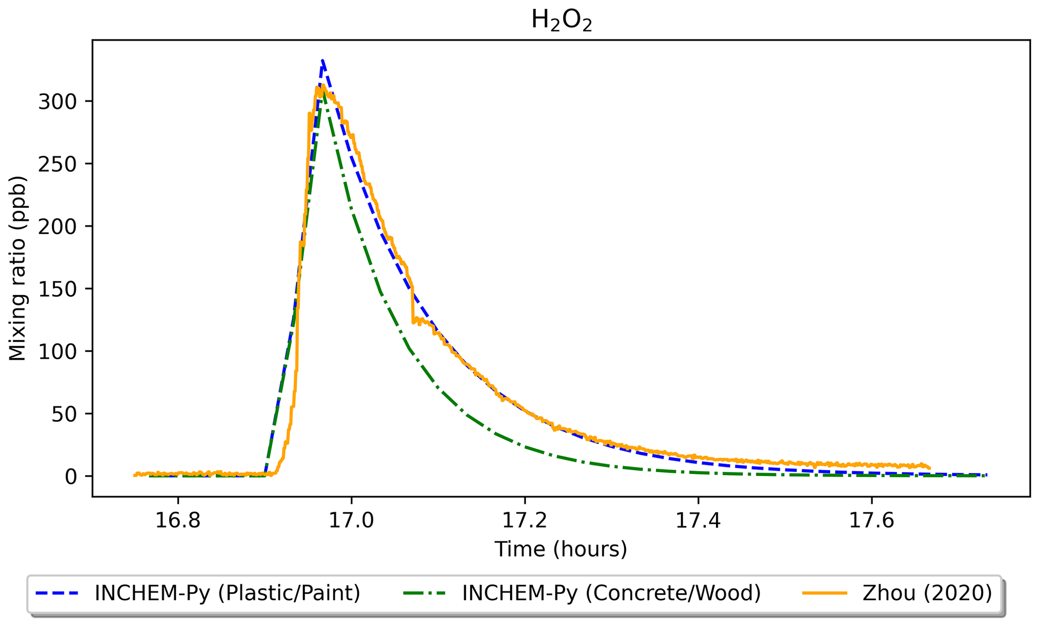
Figure 10 Comparison of experimental results of a H₂O₂ cleaning event from Zhou et al. (2020) and simulated results using INCHEM-Py.

The air change rate was constant at 0.51 ± 0.004 h⁻¹ and was sourced from outdoors, the temperature was controlled at 25.7 ± 0.9 ^∘C, and relative humidity averaged at 25.8 ± 9.5 % during the experiments. The indoor lighting was from uncovered fluorescent tubes, and a solar illuminator was used to provide outdoor lighting through the window of the experimental room. The solar illuminator removed the diurnal variation of the photolysis but not of the outdoor concentrations. In the experiment, the solar flux was measured using a spectrometer, and photolysis coefficients of key species (H₂O₂, NO₂, HONO, NO₃, O₃ and formaldehyde) were calculated and input into the INDCM. In the INCHEM-Py simulations, to account for the constant solar photolysis, the local hour angle (LHA described in Sect. 2.2) was set to 0 to give constant noon photolysis values. The indoor lighting was set to uncovered fluorescent tubes. A timed emission rate of 5.5 × 10¹⁰ $\mathrm{molec}.{\mathrm{cm}}^{-\mathrm{3}}{\mathrm{s}}^{-\mathrm{1}}$ (2.25 ppb s⁻¹) for 3 min was used to simulate the cleaning spray, based on the measured values. The surface-to-volume ratios were set to represent the experiment, and all other values were default, including the outdoor species concentrations.

Figure 10 shows the H₂O₂ mixing ratio of the experiment from Zhou et al. (2020) and two INCHEM-Py model runs – one simulating the experimental conditions of a plastic floor and painted walls (plastic/paint) and a second where the floor is changed to concrete and the walls to wood (concrete/wood). The plastic/paint scenario shows good agreement between the simulated and measured H₂O₂ mixing ratios. At peak H₂O₂ concentration, the main loss of H₂O₂ was to the painted walls (1.54 × 10¹⁰ $\mathrm{molec}.{\mathrm{cm}}^{-\mathrm{3}}{\mathrm{s}}^{-\mathrm{1}}$), followed by loss to the plastic floor and loss to outdoors (1.43 × 10⁹ and 1.16 × 10⁹ $\mathrm{molec}.{\mathrm{cm}}^{-\mathrm{3}}{\mathrm{s}}^{-\mathrm{1}}$, respectively). Compared to the plastic/paint scenario, the predicted H₂O₂ mixing ratio peaks at a lower value and drops more quickly after the cleaning in the concrete/wood scenario. This is due to a larger loss rate to the wooden walls (1.64 × 10¹⁰ $\mathrm{molec}.{\mathrm{cm}}^{-\mathrm{3}}{\mathrm{s}}^{-\mathrm{1}}$) and concrete floor (5.96 × 10⁹ $\mathrm{molec}.{\mathrm{cm}}^{-\mathrm{3}}{\mathrm{s}}^{-\mathrm{1}}$) at peak H₂O₂ concentration.

Following the cleaning event, formaldehyde is produced as a secondary product. Using INCHEM-Py, the maximum increase in formaldehyde as a result of secondary chemistry in the plastic/paint scenario was predicted to be 0.72 ppb. In the experiment (Zhou et al., 2020), the secondary emission peak was masked by the background formaldehyde concentration of over 50 ppb; therefore, this shows the importance of modelling for delineating between primary and secondary emissions. In the concrete/wood scenario, the increase in formaldehyde as a result of secondary chemistry was much higher, at 3.05 ppb. This is due to higher H₂O₂ deposition velocities and higher resulting surface emissions from concrete/wood surfaces compared to the plastic/paint combination (Carter et al., 2023).

Figure 11 Comparison of run time of the default simulation on two different computers.

4 Practical details

• URL to model: https://github.com/DrDaveShaw/INCHEM-Py (last access: 13 June 2023)

• License: GNU General Public License, v3

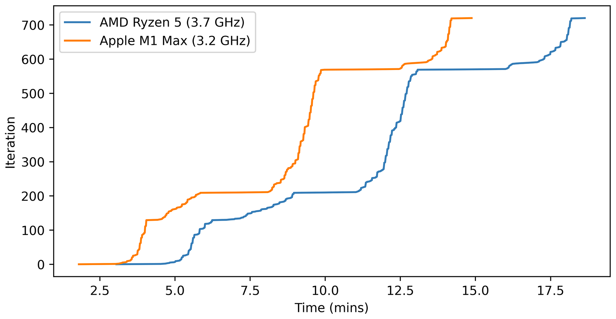
INCHEM-Py requires Python 3 and some additional packages to run. The additional packages and their known working versions are given in the user manual. The integration process is set by default to be limited to four threads, as this is the only parallelised function within the model. The number of threads can be adjusted by changing the thread pool limits in inchem_main, as described in the user manual. The default model took 18 min and 41 s on a Windows desktop with an AMD Ryzen 5 5600X 3.7 GHz processor and 14 min 54 s on an Apple laptop with a M1 Max 3.2 GHz processor. Figure 11 shows the simulation run times for these two processors. The total run time of a simulation is printed to the console at the end of the model run, and a file showing the time taken for each integration output is saved to the output folder and is included in the data set for all model runs in this paper. This function allows users to determine where the simulation may be struggling and where improvements to speed up run time might be made. In the default case, the slowest integration steps are at sunrise and sunset due to very small values for photolysis parameters when the Sun begins to rise or in the final stages of setting. Memory usage peaks at less than 2 GB for these simulations.

5 Conclusions

INCHEM-Py (the INdoor CHEMical model in Python) has been presented as a tool for the analysis and interrogation of the atmospheric chemistry of the indoor environment. We have presented the main modules developed for v1.2 within this paper and have given a further detailed description in the user manual submitted alongside. INCHEM-Py has been developed as an open and accessible piece of software, has no hidden or proprietary code, and requires minimal previous coding or modelling experience to install or run. It utilises core Python libraries, including NumPy (Harris et al., 2020) and SciPy (Virtanen et al., 2020), keeping installation of additional libraries to a minimum, and capitalising on the maintenance of the Python ecosystem.

INCHEM-Py has been validated against experimental measurements and has shown improved accuracy in comparison with the INDCM, from which it was refactored. INCHEM-Py has been developed with a focus on predicting secondary chemistry that is not feasible, or in some cases possible, to measure. Outputs of species concentrations with time are given alongside key model parameters such as surface deposition rates, seasonal photolysis rates and diurnal outdoor concentrations. Interrogating these outputs allows for a detailed understanding of the atmospheric chemical processes that occur indoors, including temporally resolved reaction rates which can be used to identify the important pathways that should be included in models with reduced chemical mechanisms (Lakey et al., 2021). For example, there are generally two types of models used to solve indoor air chemistry: box models such as INCHEM-Py that have no spatial dimensions but very complex chemical mechanisms (> 6000 species, > 19 000 reactions) and computational fluid dynamics (CFD) models that solve the evolution of very few species (< 20 species, < 15 reactions) but can track them spatially (Lakey et al., 2021). Neither model is able to fully represent the complexities of the indoor environment. The main assumption of box models is that the atmosphere is well mixed and that all species are available to react with each other at all times. However, CFD models simply cannot capture the complex chemistry of the indoor environment due to computational constraints. Each model type attempts to fill a different knowledge gap. It is up to the user to appropriately define the parameters of the models to gain the most effective insight into the processes occurring indoors (Shiraiwa et al., 2019).

The utility of INCHEM-Py is further demonstrated by the publications that have used the model since the Shaw and Carslaw (2021) release of v1.1. Published articles include Lakey et al. (2021), Wang et al. (2022), Carter et al. (2023), Beel et al. (2023) and Davies et al. (2023), with several additional articles in preparation that discuss emissions from cooking and cleaning, UV-induced emissions from plastics, and future indoor air pollution scenarios. Each case exhibits the versatility of INCHEM-Py and the ability of users to simulate custom experimental scenarios to expand our understanding of indoor air chemistry.

Future developments of INCHEM-Py will likely include an expansion of the gas-to-particle partitioning module to include more source species and prediction of particle size distributions. Chemical mechanisms and analysis tools will continue to be added as they are developed, including a Python package for the analysis of INCHEM-Py outputs. In the long term a multi-box approach may be taken to simulate adjoining spaces, or a hybrid approach may be used to add spatial dimensions.

Appendix A: Outdoor constant concentrations and source of measurements on which they are based

Uchiyama et al. (2015)Uchiyama et al. (2015)Uchiyama et al. (2015)Uchiyama et al. (2015)Uchiyama et al. (2015)Baudic et al. (2016)Uchiyama et al. (2015)Uchiyama et al. (2015)Uchiyama et al. (2015)Uchiyama et al. (2015)Uchiyama et al. (2015)Uchiyama et al. (2015)Uchiyama et al. (2015)Uchiyama et al. (2015)Uchiyama et al. (2015)Uchiyama et al. (2015)Baudic et al. (2016)Lü et al. (2006)Uchiyama et al. (2015)Uchiyama et al. (2015)Uchiyama et al. (2015)Uchiyama et al. (2015)Uchiyama et al. (2015)Uchiyama et al. (2015)Uchiyama et al. (2015)Uchiyama et al. (2015)Uchiyama et al. (2015)Uchiyama et al. (2015)Uchiyama et al. (2015)Mentese and Bas (2020)Bari and Kindzierski (2018)Bari and Kindzierski (2018)Bari and Kindzierski (2018)Uchiyama et al. (2015)Uchiyama et al. (2015)Uchiyama et al. (2015)Uchiyama et al. (2015)Mentese and Bas (2020)Mentese and Bas (2020)Sturaro et al. (2010)Baudic et al. (2016)Baudic et al. (2016)Baudic et al. (2016)Baudic et al. (2016)Bari et al. (2016)Bari et al. (2016)Baudic et al. (2016)Bari et al. (2016)Bari et al. (2016)Bari and Kindzierski (2018)Uchiyama et al. (2015)Bari et al. (2016)Bari et al. (2016)Uchiyama et al. (2015)Uchiyama et al. (2015)Uchiyama et al. (2015)Uchiyama et al. (2015)Uchiyama et al. (2015)Mentese and Bas (2020)Bari and Kindzierski (2018)Baudic et al. (2016)Baudic et al. (2016)Bari et al. (2016)Bari and Kindzierski (2018)Bari and Kindzierski (2018)Bari and Kindzierski (2018)Bari and Kindzierski (2018)Baudic et al. (2016)Bari and Kindzierski (2018)Bari and Kindzierski (2018)Bari and Kindzierski (2018)Baudic et al. (2016)Baudic et al. (2016)Gallego et al. (2016)Gallego et al. (2016)Gallego et al. (2016)Gallego et al. (2016)Hellén et al. (2018)Hellén et al. (2018)Gallego et al. (2016)Hellén et al. (2018)Uchiyama et al. (2015)Brickus et al. (1998)Bari and Kindzierski (2018)Gallego et al. (2016)Bari and Kindzierski (2018)Bari and Kindzierski (2018)Bari and Kindzierski (2018)Uchiyama et al. (2015)Uchiyama et al. (2015)Uchiyama et al. (2015)Uchiyama et al. (2015)Gallego et al. (2016)Uchiyama et al. (2015)Hakola et al. (2009)Hakola et al. (2009)Uchiyama et al. (2015)Uchiyama et al. (2015)Hellén et al. (2018)Hellén et al. (2018)Hellén et al. (2018)Hellén et al. (2018)He et al. (2010)Hellén et al. (2018)Dlugokencky (2022)EEA (2018)EEA (2018)EEA (2018)EEA (2018)EEA (2018)Vichi et al. (2016)Vichi et al. (2016)Li et al. (2018)Liu et al. (2018)EEA (2018)

Table A1 Outdoor constant concentrations used in INCHEM-Py including the references used to obtain the v1.2 values. Values given as “Average” are averages of the diurnal profiles used in the model. The cited values are taken from multiple papers covering multiple locations, times of year and lengths of study that may or may not be applicable to individual user requirements. A summary of these details is given in Table A2.

Uchiyama et al. (2015)Baudic et al. (2016)Lü et al. (2006)Mentese and Bas (2020)Bari and Kindzierski (2018)Sturaro et al. (2010)Bari et al. (2016)Gallego et al. (2016)Hellén et al. (2018)Hakola et al. (2009)He et al. (2010)Dlugokencky (2022)Vichi et al. (2016)Li et al. (2018)Liu et al. (2018)

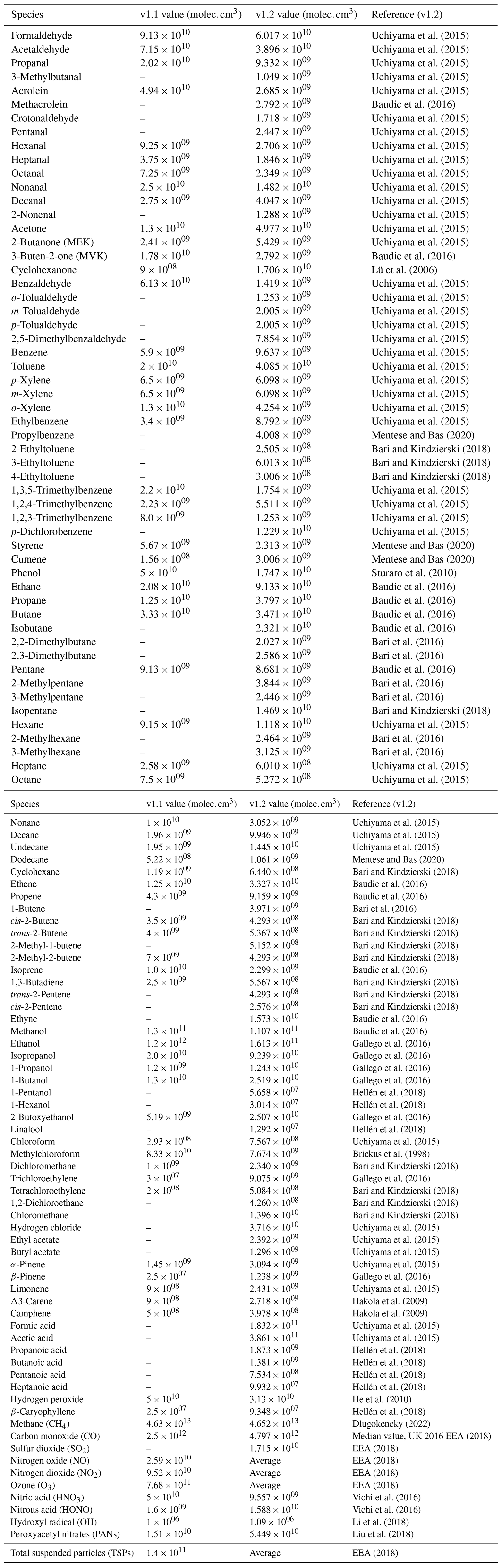
Table A2 Locations, times of year and lengths of study for literature used to update outdoor concentrations in INCHEM-Py v1.2.