Deciphering past earthquakes from the probabilistic modeling of paleoseismic records – the Paleoseismic EArthquake CHronologies code (PEACH, version 1)

A key challenge in paleoseismology is constraining the timing and occurrence of past earthquakes to create an earthquake history along faults that can be used for testing or building fault-based seismic hazard assessments. We present a new methodological approach and accompanying code (Paleoseismic EArthquake CHronologies, PEACH) to meet this challenge. By using the integration of multi-site paleoseismic records through probabilistic modeling of the event times and an unconditioned correlation, PEACH improves the objectivity of constraining paleoearthquake chronologies along faults, including highly populated records and poorly dated events. Our approach reduces uncertainties in event times and allows increased resolution of the trench records. By extension, the approach can potentially reduce the uncertainties in the estimation of parameters for seismic hazard assessment such as earthquake recurrence times and coefficient of variation. We test and discuss this methodology in two well-studied cases: the Paganica Fault in Italy and the Wasatch Fault in the United States.

1 Introduction

A principal challenge in paleoseismic research is having complete and properly time-constrained paleoearthquake catalogues. The presence of large sedimentary hiatuses due to depositional intermittency, imbalanced erosion–deposition rates, or scarce availability of datable material are common limitations leading to poor age control in trenches. These uncertainties in the event age constraints add to the difficulty of site correlations and hence in establishing a reliable paleoearthquake chronology representative of the whole fault.

To assess the correlation problem, two approaches have been developed (Fig. 1a and b). The first one (DuRoss et al., 2011) addressed this issue in a segment of the Wasatch Fault (United States) by correlating site chronologies computed with the Bayesian modeling software OxCal (Bronk Ramsey, 2009, 1995). After an overlap analysis of the event probability density functions (PDFs) among sites, the correlation (product of PDFs) was restricted between the PDF pairs that showed the highest overlap at each site (Fig. 1b). This model demonstrated a reduction in event time uncertainties and refined the chronology of the Wasatch Fault but carries some limitations. First, basing the correlation on PDF overlaps can be problematic in other datasets with larger uncertainties, where one event PDF at a site may partially or fully overlap with more than one event PDF at another site (Fig. 1b). Second, it can hamper the ability of identifying additional events that might not have ruptured at all sites; for instance, PDFs at different sites that overlap but that are skewed in opposite directions could be in fact two different events. In these cases, restricting correlation to individual events can reduce the accuracy of the analysis.

Figure 1 Schematic comparison of the existing approaches to correlate paleoseismic sites with our method. The example is artificial. (a) Method by Cinti et al. (2021) using a non-probabilistic modeling of event times. The sweep line algorithm moves from left (older times) to right (younger times) and evaluates the intersections between events at each site. The outcome in the example are two possible correlation hypotheses (middle and bottom panels). This figure is originally drawn for the present example but based on the method illustrated by Cinti et al. (2021). (b) Method by DuRoss et al. (2011) using event times modeled as probability density functions (PDFs) in OxCal. This method analyzes the overlap between PDFs and correlates those with higher overlap. In the example of the middle panel, the two younger (right) PDFs of sites 1 and 2 are correlated, and the older (left) one at site 2 is left alone as a single-site event. The final chronology (bottom panel) consists of the product PDF between the two correlated PDFs at sites 1 and 2 (E2) and the un-correlated PDF of site 2 (E1). The PDF shapes of the two top sub-panels are drawn from the OxCal models provided in the supplements of DuRoss et al. (2011). (c) Method in this study. We also consider event times modeled as PDFs but, instead of imposing which PDFs are correlated, we compute the average distribution of all PDFs (middle panel). Then, the peaks of probability in this distribution (considered as event occurrence indicators) are used to extract all event PDFs intersecting its positions (dashed lines) and are multiplied into a product PDF. This allows one event PDF to participate in more than one correlation: for instance, the event at site 1 is intersected by both peaks 1 and 2 and therefore participates in the computation of both E1 and E2 product PDFs. This unrestricted correlation accommodates the possibility of the event at site 1 being two events, as supported by its overlap with both events at site 2.

More recently, Cinti et al. (2021) developed an approach to model earthquake occurrences from paleoseismic data at the fault system scale in Central Italy. In this case, their approach does not model events probabilistically but considers equal occurrence likelihood throughout the whole uncertainty range of the event time (Fig. 1a). Using a sweep line algorithm, their approach explores scenarios of event correlation between sites within the same fault and along the whole fault system to identify potential multi-fault ruptures. This algorithm passes a vertical line along the time axis and searches all intersections between event times among sites, providing the list of correlation hypotheses (Fig. 1a). Besides the differences in the event time modeling, the approximation followed for site correlations is similar to DuRoss et al. (2011) in the sense that, for each scenario, only one event correlation hypothesis is considered. Although a set of scenarios with all correlation combinations are explored, the authors ultimately set their preferred ones based on expert judgment. Again, this is not the ideal solution when event ranges highly overlap because ranking scenarios become highly subjective, and working only with the event time ranges (without probabilities) adds further difficulty to this task. On top of this, both methodologies are developed for case-specific needs, so their applicability to other settings might be diminished, especially where paleoseismic data are less well-constrained and scarcer than for the tested faults.

To accommodate the mentioned limitations, we present a new approach and accompanying code named PEACH (Paleoseismic EArthquake Chronologies). Its main purpose is to probabilistically compute paleoearthquake chronologies in faults based on an objective and unrestricted correlation of paleoseismic data, accounting for common problematic situations inherent to paleodata and reducing uncertainties related to event age constraints. This makes it flexible in terms of its applicability to other datasets worldwide. PEACH relies on (i) simple and easy to compile inputs, including the option of using chronologies computed with OxCal; (ii) a semi-automated workflow; and (iii) outputs that can be further used to compute fault parameters for the hazard (e.g., earthquake recurrence intervals or coefficient of variation). To demonstrate and discuss the advantages of the method, we show applications in two real-case examples in Central Italy and the Wasatch Range in the United States.

With PEACH we aim to introduce a reliable and objective tool to interpret multi-site paleoseismic data and to characterize the earthquake occurrences on faults, especially when the uncertainties or amount of data prevent establishing clear interpretations manually. Additionally, the approach can give insight into the spatial extent of the paleosurface ruptures along a fault.

2 Fundamentals of the approach

It can be assumed that, because earthquake ruptures can be recorded at more than one site of a fault, it should be possible to identify correlations in paleoearthquakes between trenches along that fault. Furthermore, the differences in time constraints from site to site can help us to better constrain the final event chronologies representative of the whole fault (e.g., DuRoss et al., 2011). Based on this assumption, the approach adopted herein is based on two main premises:

• a.

  Correlations are restricted to the fault level, defined as in the Fault2SHA Central Apennines Database (CAD) (Faure Walker et al., 2021). According to that, a fault is a singular first-order structure that has the potential of rupturing the entirety of its length and with prominent end boundaries that can cause ruptures to stop. A fault can be formed by smaller sections (traces) with different levels of activity evidence or location certainty that do not constitute sufficient barriers for rupture propagation. Fault-to-fault correlations have not been tested yet in the approach, as they require a series of fault conditions (e.g., geometrical or physical; Boncio et al., 2004; Field et al., 2014) that are not applicable to all settings and need to be implemented cautiously.

• b.

  Trench paleoearthquake records are always a minimum; hence, the wider the uncertainties in event times, the higher the chance of underdetection. Along this reasoning, when an event at a site fully or partially overlaps in time with several events in another, the correlation is not favored to any of the possible combinations. Instead, all correlation combinations are allowed simultaneously by integrating all event probabilities, as we explain further in the paper.

3 Data and workflow

PEACH is based on a code written in MATLAB (https://www.mathworks.com, last access: March 2023) that probabilistically models event times from paleoseismic data on a fault to derive its paleoearthquake chronology. Such data need to be compiled into a series of inputs detailed below. The current version (version 1) of the code is available in the Zenodo repository of the article (Gómez-Novell et al., 2023).

3.1 Input data

The PEACH code relies on two simple input files. The first file (e.g., faultname.csv; Table 1a) contains a list of all paleoearthquakes classified by each site in the fault and the dates limiting their younger and older age bounds. The dates correspond to the calibrated numerical dates that limit the event horizons in the trenches (Fig. 2a) and should be provided following the before common era and common era notation (BCE/CE). The second file (site specifications, site_specs.txt; Table 1b) specifies a series of calculation information (e.g., sigma level truncation or number of random samples/seed) and allows the oldest and youngest dates for the exposed stratigraphy in each fault to be set in case these are not available in the datasets.

Table 1 Input data required for the calculation with PEACH. (a) Main input file containing the paleoseismic events and limiting dates for the example of fault R in Fig. 2a (file faultR.csv in the “Inputs” folder in the code's Zenodo repository; Gómez-Novell et al., 2023). Events are sorted from youngest to oldest at each site, and the dates (and corresponding samples in brackets) represent the age of the units limiting the event horizon in the trenches: “Event_date_old” is its older constraint and “Event_date_young” the younger age constraint. Error columns represent the 1σ uncertainties of the numerical dates. Dates should be provided with the before common era and common era notation (BCE/CE): negative for BCE and positive for CE. “Null” means not available. (b) Example of the site specification file of fault R in Fig. 2 (site_specs.txt in the “Inputs” folder). The “sigma_level” allows us to truncate the PDFs and work only with significant sigma levels: 1 for 1σ, 2 for 2σ, 3 for 3σ, and 0 for full σ. See text for details on when this truncation is recommended. The “oldest_faulted” corresponds to the oldest available date affected by faulting. The code uses this date in the cases when the oldest age bound of the first event in a trench is not available in the first file (Null). If not provided in the “site_specs” file, the code automatically assigns the date of the oldest faulted materials along the whole fault. The “oldest_unfaulted” is the oldest available date not affected by faulting (e.g., the younger age bound of the last event). This might correspond to the maximum age for surface ruptures in the historical catalogue of a study area. If this date is not provided when needed, an error is returned. Otherwise, if there are no dates missing in the dataset, the mentioned fields should state “nan”. The “seed” is the number of samples that the code iterates in each limiting numerical date to compute the event PDF (see text for details). All mentioned parameters except for the truncation level are skipped by the code when working with OxCal chronologies as inputs.

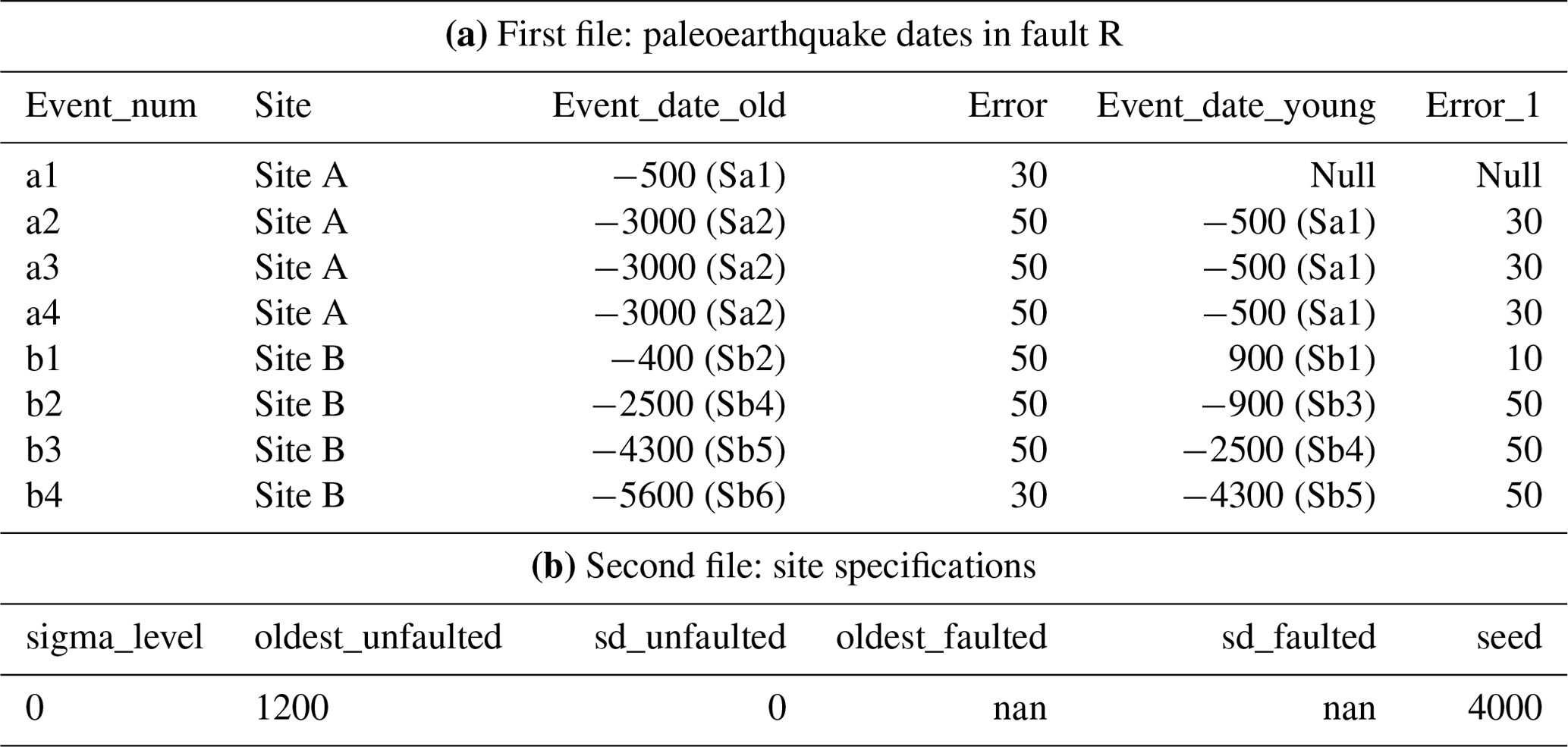
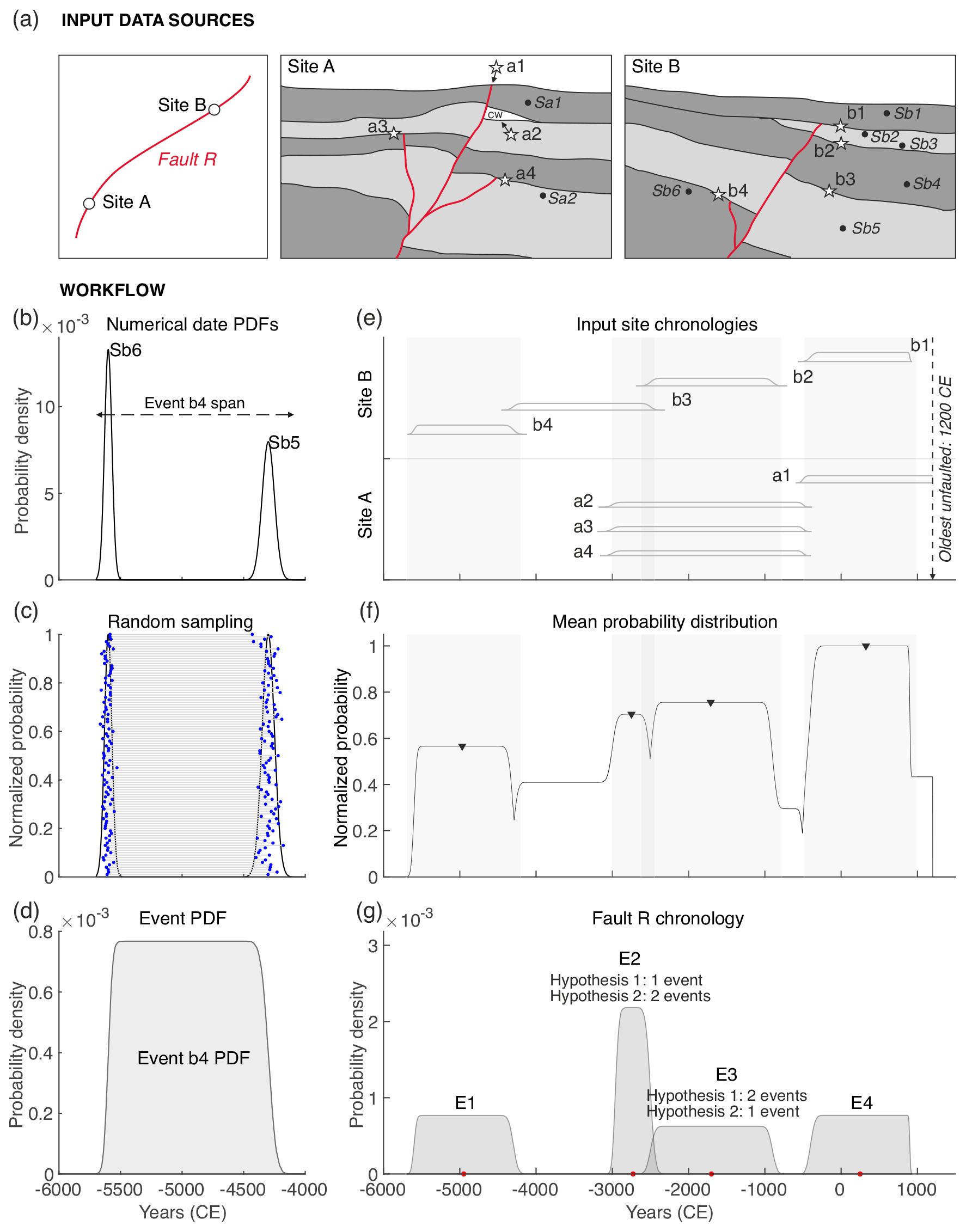
Figure 2 (a) Trench logs of the artificial fault R at two paleoseismic sites (sites A and B). Stars indicate the event-horizon locations in the trenches. Each paleoseismic trench has four paleoseismic events recognized: events a1 to a4 at site A and events b1 to b4 at site B. The numerical dates of the limiting units (Sa1 and Sa2 at site A and Sb1 to Sb6 at site B) are available in Table 1a. Note that the insufficient date availability at site A limits the capability of constraining individually the dates of events a4 to a2; all three events have the same age limits (Fig. 2e). CW: colluvial wedge. (b) Conversion of the numerical dates and 1σ uncertainties of the input table (Table 1a) into normal PDFs. The dates limiting event b4 are taken as an example. (c) Random sampling (100 samples depicted here) of the numerical dates (dots) and establishment of time ranges between them (horizontal gray lines). (d) Event b4 PDF resulting from adding all time ranges and scaling them so that the sum of the probabilities equals 1. (e) Input site chronologies of sites A and B with the event PDFs depicted. The gray bands indicate the 2σ ranges of the final chronology in panel (g). The historical limit (oldest unfaulted date in the site specifications input file; Table 1b) is the age above which the seismic catalogue is complete for the surface ruptures in the region. Here we test a hypothetical date of 1200 CE. (f) Mean distribution and detected peaks resulting from averaging all event PDF probabilities in the studied time span. The gray bands indicate the 2σ ranges of the final chronology in the next panel. (g) Final chronology for fault R with the mean value (dot) indicated for each PDF. Note that, because events E2 and E3 cover a time span when three events have the same age constraints at site A, there are two mutually exclusive hypotheses of event count that are provided for each PDF: if one hypothesis considers E2 as being one event, then E3 should correspond to two events and vice versa. In all cases the total count of the whole chronology is five events contained in four PDFs.

OxCal paleoearthquake chronologies

Nowadays, most paleoseismic studies use OxCal to compute site chronologies not only because it allows the user to statistically model complex stratigraphic sequences with sometimes conflicting numerical date distributions, but also because it allows us to impose a series of conditions to date events based on expert geological observations, i.e., skewing the event PDF towards a limiting date due to the presence of coseismic evidence (e.g., colluvial wedges). To allow the preservation of such expert rationales for the correlation, our code also accepts event PDFs computed and exported from OxCal instead of the previously explained input. To do so, the PDFs of all sites expressed as probabilities versus time need to be provided in a single input file following a similar format to the one provided by OxCal.

For information on the OxCal input file preparation check the PEACH user manual available in the Zenodo repository of this paper (Gómez-Novell et al., 2023). There you will also find all the input files used for the calculations in this paper.

3.2 Workflow

The PEACH source code is structured in four consecutive steps that are executed automatically. Note that, in the case of using chronologies computed with OxCal, the first step of the workflow is skipped.

• i.

  Building individual event PDFs. The individual event PDFs (referred to as “event PDFs” throughout the remaining text) are built from the trench numerical dates that limit each event horizon (Fig. 2c). First, the numerical dates are transformed into normal PDFs. The choice of using normal distributions, aside from simplicity, was made to accommodate luminescence dates, which usually are expressed as normal distributions. These types of dates are more prevalent at sites dominated by older, coarser, or less complete deposits – inherently more challenging to date accurately using other, more precise techniques like radiocarbon. It is in these contexts that site correlation poses a bigger challenge, making our approach particularly valuable.

  Second, for each pair of numerical dates that limit an event, a random sampling of “n” iterations is performed based on the event probabilities, and “n” time ranges are established between sample pairs (Fig. 2c). The number of random samples (seed in the site specification file; Table 1b) is set after a sensitivity analysis that explores the change in the average PDF probabilities as a function of the increment of random samples in the PDF computation. For the datasets explored in this paper, the seed is set at 4000 samples because it ensures a stable modeling of the probabilities and implies minor changes in the computed average PDF probabilities with respect to larger seed increases (see Fig. 3 and the synthetic example of Table 1a and the Paganica Fault in Central Italy; Table 2a). In addition, a seed of 4000 was found appropriate for other tests performed during development of the code. Although we estimate that the 4000-sample default seed is conservative enough to work properly in most datasets, ideally, we recommend the seed value to be determined for each dataset through the sensitivity analysis proposed. This is important because poor sampling in the PDF computation can lead to instable PDF modeling, meaning diminished repeatability of the model runs. The stability of the PDFs can be verified in two ways: (1) by running PEACH over various seed values and analyzing the chronology variations afterwards or (2) by pre-running a separate analysis before the main PEACH computation. This latter analysis (i.e., the one shown in Fig. 3) can be performed through a MATLAB code that is available in the Zenodo repository of this paper (Gómez-Novell et al., 2023). Check the user manual in the repository for guidance.

  Lastly, all time ranges computed are added to derive the event PDF and scaled so that the sum of all probabilities per PDF equals 1 (Fig. 2d). This process is done for all events and all sites analyzed in the fault.

• ii.

  All-site PDF average. A mean probability distribution is computed by averaging the maximum probabilities of the event PDFs from each site and for each year time bin. The maximum is used, so the average outlines the maximum probability areas of each event PDF to avoid peaks in PDF intersections. This average distribution depicts the overall earthquake occurrence probabilities in the fault for the time span observed (Fig. 2f). Because the probability (height) of each event PDF is inversely proportional to the width of its uncertainties, the better-constrained events make a higher contribution (i.e., higher height) to the average distribution. The peaks of probability in this distribution are thus assumed as an indicator of a higher earthquake probability of occurrence. Their detection and time location are therefore crucial to derive the chronology.

• iii.

  Probability peak detection. The peaks of the mean distribution are detected based on their prominence, which measures how much the peak's height stands out compared to the rest of the peaks in the distribution. First, a reference base level is set at the local minimum in the valleys around each peak, and then the prominence is measured from this level to the peak value. To avoid noisy detections and underdetection, a minimum prominence threshold (minprom) is set above which all peaks should be detected.

  The target parameter to define the minprom is the minimum peak probability (minP) of the event PDFs, namely the PDF with the widest uncertainty of them all (Fig. 4a). Because the mean distribution is normalized, the minP value is also normalized using the maximum probability of all PDFs (maxP; Fig. 4a). This normalized quotient is then divided by 4 to account not only for the minprom being detected in the mean distribution (i.e., whose probabilities are $\mathrm{1}/\mathrm{2}$), but also for the instances in which two different PDFs overlap significantly so that they generate a flattened mean distribution with peaks that have prominences smaller than half their maximum probability. See Eq. (1):

  $$\begin{array}{}\text{(1)}& \mathrm{minprom}=\mathrm{0.25}\times (\mathrm{minP}/\mathrm{maxP}).\end{array}$$

  The peak detection works also in plateau-shaped peaks (e.g., Fig. 2f), where the peaks are placed in the median point of the plateau instead of its corners (default). This is achieved by running the detection function twice in opposite directions in the timescale (left to right and right to left) and computing the median value between the corners to set the peak.

  The minprom threshold is one of the most important parameters in PEACH as it controls the locations where the final chronology will be extracted and computed (see next step); therefore a correct detection of the peaks is crucial for the correct performance of the modeling. As such, the method involves a series of refinements in case of poor performance of this parameter (see Sect. “Refinements of the chronology”).

• iv.

  Extraction of the paleoearthquake chronology. The peak locations do not correspond to the final event times; they indicate times of higher event likelihood (i.e., higher event overlaps) in the fault's timeline, which need to be translated into distributions that probabilistically express the event timing in each peak position. To do so, all the event PDFs from all sites that intersect each peak position (Fig. 2e) are correlated (multiplied) into a product PDF (i.e., final PDFs). The product operation is used because (i) it places the higher probability of the final PDFs at the overlaps of the input PDFs, which is where the events are most likely located, and (ii) it reduces the uncertainties of these final PDFs compared to the input chronologies (e.g., Fig. 2e versus 2g).

  The set of product PDFs represents the final chronology of the fault (Fig. 2g). Note that two event PDFs can participate in more than one product PDF if they intersect more than one peak position (Figs. 1c and 2e). Also note that, given the random nature of the PDF computation process, the same input data might yield slightly different results in each calculation.

Refinements of the chronology

After the extraction of the paleoearthquake chronology, four types of problematic situations linked to the data used to build the model may arise, requiring further refinements. These refinements are necessary to produce a more reliable and realistic chronology, as explained below.

• a.

  Overlapping event PDFs. At some sites, the lack of age constraints can yield age ranges of consecutive events that overlap highly in time or even show the same exact age (e.g., three older events at site A; Fig. 2e). Such an overlap makes it difficult to produce a mean curve with individual peaks corresponding to each event and therefore can mask events in the final chronology. To solve this, for each final PDF, the code identifies the sites where these overlaps occur and counts them. The outcomes are final PDFs that can represent the occurrence of more than one event. The number of events that each PDF represents corresponds to the maximum number of overlaps identified at any site at that time position. If there is more than one final PDF in the time span covered by the overlapping events, the number “N” of such overlapping events is divided between the number of PDFs. If the division is odd, all event combinations that add to “N” are generated (E2 and E3; Fig. 2g).

• b.

  Peak overdetection. In some cases, the prominence threshold might not be high enough to avoid noisy detections (Fig. 4). In this case the code is prepared to automatically clear out repeated final PDFs in the chronology that come from peaks very close in time (e.g., peak clusters in jagged-shaped peaks; Fig. 4).

• c.

  Peak underdetection. This is mostly related to an unsuitable (too high) prominence threshold value in the dataset analyzed. A general rule of thumb for the user to identify underdetection is to determine whether the number of peaks detected by the code is lower than the number of events identified at the most populated paleoseismic site in the dataset. If this is the case, there are a series of causal scenarios of the underdetection that can be addressed and fixed. One cause can be related to the poor peak definition due to a large overlap between the PDFs of the dataset. For such cases, the user has the option to truncate the event PDFs to different levels of statistical confidence (sigma), which can help by increasing the peak prominence.

  Another cause is datasets that contain known historical or instrumental ruptures, which can also fall in the underdetection problem. These events have no timing uncertainties, and, therefore, their peak probability equals 1. Conversely, paleoseismic datasets have larger uncertainties and therefore much smaller peak probabilities on the order of $\mathrm{1}\times {\mathrm{10}}^{-\mathrm{2}}$ to $\mathrm{1}\times {\mathrm{10}}^{-\mathrm{3}}$ or less (e.g., Fig. 2d). The combination of both types of datasets in a calculation generates a mean distribution whose shape is controlled by these historical peaks, while the paleoseismic events show practically negligible prominences. This scale contrast flattens the normalized mean distribution in the regions where event PDFs have small prominences (poorly constrained; usually the older parts of the records) and thus can go unnoticed by the code given the minprom threshold set. In such cases and if the target is to increase the resolution of the older paleoseismic record, we recommend leaving historical events out of the computation.

  Finally, although remote, we cannot ignore the possibility that for some datasets the prominence threshold does not work properly even with the application of the mentioned fixes. If that is the case, the threshold might require manual tuning inside the code. In that case we recommend checking the user manual for guidance (Gómez-Novell et al., 2023).

• d.

  Event PDFs with wide codas. In such instances, the lower probabilities (close to 0) of the coda regions might interfere in the computation of the product PDF by overconstraining them compared to the original datasets. In addition to the overconstraining, the wide codas of PDFs can cause an incorrect clearance of the overdetection because they can intersect peaks located farther in time from their higher-probability region. For the example in Fig. 4, two clustered peaks of the same height in the mean distribution correspond to the same event, but one of them is redundant. Because they are so close in time, in ideal conditions they will intersect the same event PDFs and yield the same final product PDFs, making it easy for the code to clear out the repeated event. However, if one of the two peaks is intersected by a wide coda of a farther PDF (a PDF that does not contribute to the probability high analyzed), the product PDFs computed will not be identical and therefore the code will interpret those two redundant peaks as two different events. Working with sigma-truncated event PDFs can help us both to exclude the low-probability regions for the noise clearance (Fig. 4b) and to improve the overconstraining of certain PDFs.

  Check the user manual (Gómez-Novell et al., 2023) for details and examples on the situations explained for the refinements.

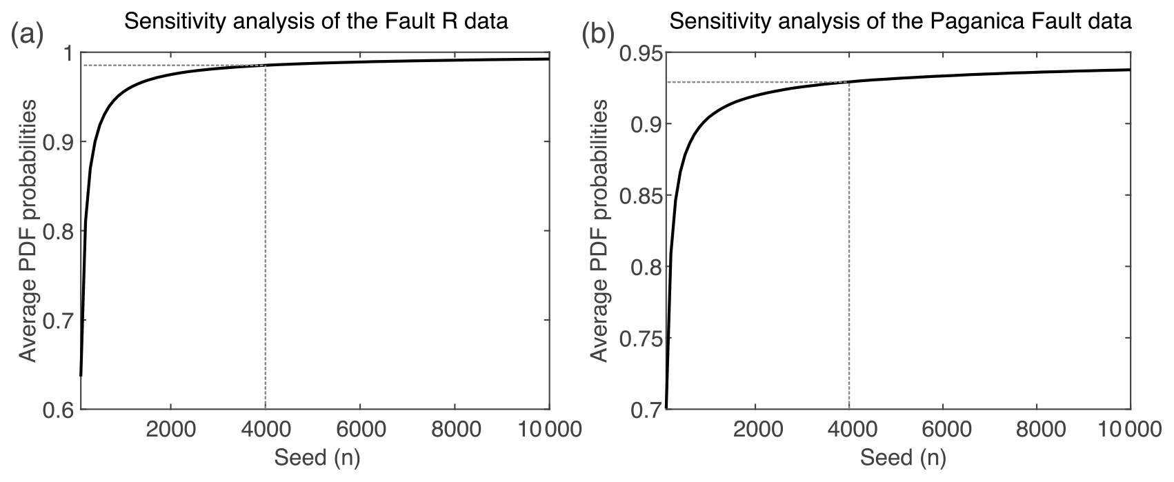
Figure 3 Sensitivity analysis for the number (n) of random samples (seed) explored within the numerical date PDFs to build the event PDFs for the (a) synthetic example of fault R depicted in Fig. 2 and (b) the Paganica Fault depicted in Fig. 5. The seed sensitivity is analyzed with respect to the global mean of all the mean event probabilities in the respective fault datasets. For smaller seeds below ∼ 4000 samples the average probabilities are highly variable. Above this value, increasing seeds lead to small changes in the PDF probabilities as the curve gets asymptotic, while computation time increases. For the Wasatch Fault System example this analysis is not performed because the event PDFs are taken from previously computed OxCal chronologies (see Sect. 4.2).

Figure 4 Definition of the parameters to calculate the prominence threshold (minprom; Eq. 1) and noise removal workflow in a simplified dataset of two event PDFs. (a) Chronology computation with non-truncated (full σ) PDFs. In the upper panel minP and maxP are defined as the minimum and maximum peak probabilities of the PDFs in the dataset, respectively. Note here that the less-constrained PDFs have a coda that intersects the better-constrained one. The middle panel shows the next step in which all PDF probabilities are averaged, and the probability peaks are detected based on the minprom, as defined by Eq. (1). Note that for the PDF on the right, the jagged shape leads to two peaks, one located at the true probability peak of the PDF and another that can be interpreted as noise. Because the chronology is extracted based on the peak positions, the final PDFs (products) computed for both peaks are different because the noise peak intersects the coda of the neighboring PDF and the true peak does not. This computes an extra event (E2) that is, in fact, an artifact of the noise combined with a poorly constrained PDF and, as such, overestimates the event count: three events instead of the two observed. (b) Chronology computation with PDFs truncated at 2σ. In this case the truncation removes the coda intersection and the final chronology shows two events, consistent with the observed.

3.3 Outputs

Two types of outputs are generated. The first outputs are two csv files (“Final_PDFs.csv” and “Final_ PDFs_stats.csv”) containing (i) the final PDFs expressed as probabilities as a function of time and (ii) statistical parameters of the PDFs (mean and standard deviation), respectively. These files also provide the number of events contained in each PDF in case of overlaps (e.g., hypotheses 1 and 2 in Fig. 2g). The second output (Final_PDFs.pdf) consists of three visualization figures: (i) the event PDFs at each site (Fig. 2e), (ii) the mean curve with the peak identification (Fig. 2f), and (iii) the final chronology (Fig. 2g). Besides visualizing the modeling results, the output figures can be used to identify the sites correlated for each event and therefore to infer geospatial attributes such as rupture length and fault segmentation hypotheses (e.g., boundary jumps). All the output files of the examples shown in this paper (fault R, Paganica Fault, and Wasatch Fault Zone) are available in the “Outputs” folder of the code's Zenodo repository of the paper (Gómez-Novell et al., 2023).

Aside from the output files, the code produces a summary in the command window that informs the user of the number of events identified in the chronology, the uncertainty reduction compared to the input chronologies, and an estimation of the mean recurrence time and coefficient of variation (CV) of the chronology. The recurrence and CV values, estimated arithmetically from inter-event times, are intended to be indicative and should be taken with caution, especially because some datasets might have completeness issues in the older parts of the sequences that can highly impact their reliability. For a more statistically robust computation and treatment of the uncertainties in the recurrence and CV, we recommend using the outputs of PEACH in other software programs such as “FiSH” (Pace et al., 2016), which are specifically designed for this purpose.

4 Applications to real cases

We show the application of PEACH in two datasets from two different tectonic contexts worldwide: the Paganica Fault in Central Italy (Fig. 5) and the Weber Segment of the Wasatch Fault System in the United States (Fig. 6). These faults are selected because they are well studied at multiple sites along their traces and, consequently, have populated paleoseismic records that are optimal to put the method to the test. Furthermore, the fact that paleoseismic studies in the Wasatch Fault System have relied on OxCal modeling enables us to show the results of the approach also using such chronologies as inputs. Conversely, the artificial example shown in Fig. 2 demonstrates how the methodology is also able to work in simpler and less populated datasets.

4.1 Paganica Fault

The Paganica Fault is an active normal fault accommodating NE–SW extension in the Central Apennines (Italy) and was responsible for the devastating 2009 L'Aquila earthquake sequence, as demonstrated by seismic (e.g., Chiarabba et al., 2009) and coseismic surface rupture data (e.g., Falcucci et al., 2009; Boncio et al., 2010; Roberts et al., 2010). The Paganica Fault used in this example is the one defined in the CAD database (fault level; Faure Walker et al., 2021), composed of nine traces, all of which demonstrated the capability of rupturing simultaneously during the 2009 event. The fault level considers first-order structures that can rupture entirely but with prominent end boundaries able to stop ruptures from propagating further.

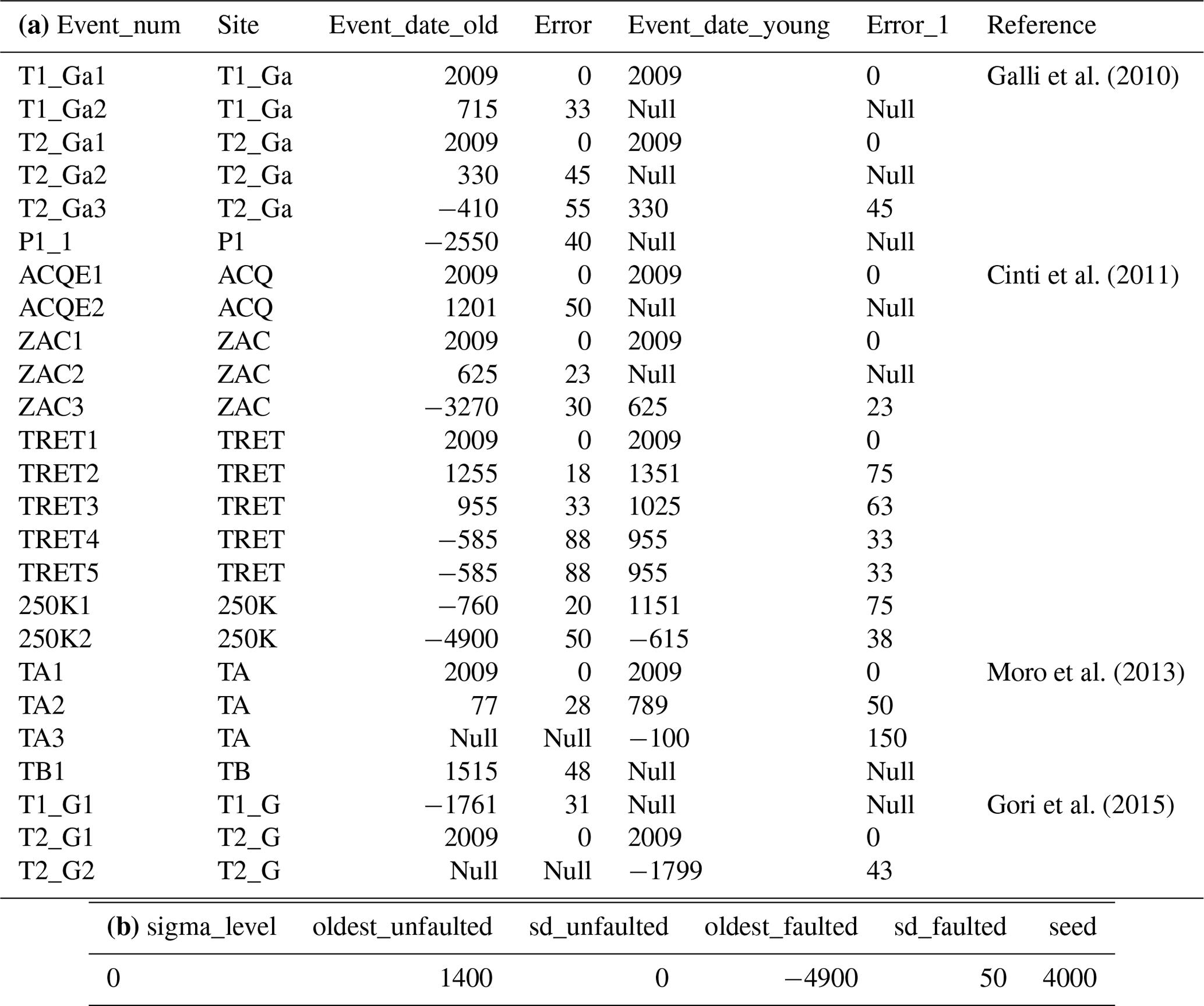
We compiled the published paleoseismic data from the 11 paleoseismic sites (Table 2a) studied along the Paganica Fault, with a total of 25 paleoearthquakes defined by the numerical dates limiting each event horizon (Table 2a). Two additional paleoseismic sites (Trench 3 by Galli et al., 2011, and Trench C by Moro et al., 2013) have been excluded from this analysis due to the lack of numerical dates to establish a paleoearthquake chronology.

The compilation of the paleoseismic data implied a bibliographic revision in which we re-defined the age constraints of the events in those cases when the authors introduced expert judgments (e.g., assign a discrete historical date to an event based only on the fact that its time range covers the timing of that historical event). Far from questioning the interpretations by the authors, this is done to ensure as objective a dataset as possible based only on independent numerical data. The criteria followed in the compilation are that the numerical dates selected to define the event time constraints are always (i) the ones closer to the event horizons and (ii) the ones that have stratigraphic coherency. A series of conditions are applied:. (a) The same age constraints are assigned to events that cannot be dated individually. (b) The surface rupture data here are considered complete from 1400 CE onwards, as suggested by Cinti et al. (2021) for the catalogue in Central Italy. Therefore, this date is considered the “oldest unfaulted” date, prior to the 2009 L'Aquila earthquake, to be assigned when the youngest bound of the last event in a trench is not available (Table 2b). However, this completeness value is not definitive, and other dates could be tested.

The chronology of the Paganica Fault is computed considering 4000 random simulations (seed) based on the sensitivity analysis of Fig. 3.

Table 2 (a) Input data and related references of the Paganica Fault as used in this study. Notes: the model resulting from these data is shown in Fig. 5. “Null” indicates that the age bound of that event has no date available in the dataset. Therefore, the “oldest_unfaulted” and “oldest_faulted” parameters from the site specifications (b) are used to assign a date to the respective younger and older missing event limits. The first is assigned 1400 CE as explained in the text. The second is assigned the oldest date available in the dataset as a conservative bound (4900 ± 50 years BCE from the 250K site). Dates are in the BCE/CE notation: negative for BCE and positive for CE.

Results

Our approach computes six final PDFs along the entire Paganica Fault, including the 2009 L'Aquila earthquake (Fig. 5) whose geological effects were observed in many trenches. The final chronology is better-constrained compared to the chronologies of the individual sites, as demonstrated by the average of the 1σ uncertainties of the event PDFs (∼ 550 years) with respect to the mean of those of the final PDFs (∼ 40 years). This represents a ∼ 93 % reduction in the average uncertainties, although this should not be directly translated into a measure of the quality improvement of our model, especially in the older part of the sequence.

Before the CE, the site chronologies are generally poorly constrained. In this regard, our probabilistic modeling shifts the timing of the first event (E1) towards the better-constrained (younger) part of the chronology (Fig. 5c), based mainly on the correlation with the older events at the T2_Ga and TA sites (Fig. 5a). Although its timing is coherent with the data, its real uncertainty should be considered higher towards BCE times. For this same reason, for BCE times, our method is not able to extract a chronology because the wide uncertainties generate poor definitions in the average distribution for the peak identification (Fig. 5b). Moreover, the fact that the Paganica Fault dataset includes the 2009 event changes the shape (prominences) of the mean distribution and likely reduces even more the code's capability to detect events in the older part of the sequence. This is because the 2009 event has no uncertainty, and therefore, its probability is maximum (equal to 1), as opposed to the much lower probabilities generated by older events (Fig. 5b).

The Paganica Fault final chronology increases by one the number of events identified by Cinti et al. (2011) at the most populated site along the Paganica Fault (TRET) for the past 2500 years. We attribute this additional event to the correlation with observations at other sites and to the probabilistic modeling of event times, whose peak probability locations can allow an increased resolution of the paleoearthquake record. For instance, the last two penultimate events, E4 and E5, are identified thanks to the different positions of the peak probabilities of the last event PDFs at sites TRET and TB, respectively (Fig. 5a). Excluding the probabilities, the event time spans would not be sufficient criteria to confidently correlate them as two events because of their considerable overlap (>50 % of the range of the event in TB). That is, in fact, the interpretation by Cinti et al. (2021) using the same dataset as ours: two penultimate events, one between 1461 and 1703 CE (equivalent to our E5) and another one between 950 and 1050 CE (equivalent to our E3). The PDF of the last event at the TRET site allows us to also identify E4.

In general, the results we obtain for the Paganica Fault are coherent with those already published. Our modeling allows us to refine the event identification and to improve the constraints of the event timing uncertainties, which is important for a more reliable characterization of fault parameters such as the average recurrence interval and coefficient of variation.

Figure 5 Results of the application of our approach to the Paganica Fault using paleoseismic data from 11 sites (see Table 2). (a) Input site chronologies for all sites studied, including the 2009 L'Aquila earthquake (dots). The locations of the sites along the Paganica Fault trace are indicated to the right. The location of the Paganica Fault within the Central Apennines is indicated in the inset in the lower-right corner of the figure. Only the chronologies for the past 2500 years are depicted in the figure because they are the ones that allowed us to compute the final chronology (see text for details). PDFs are scaled so that their probabilities add to 1 (wider uncertainties mean less probability and height). The gray bands indicate the 2σ ranges of the final chronology in panel (c). Fault traces are extracted from the Fault2SHA Central Apennines Database (Faure Walker et al., 2020). (b) Mean distribution resulting from the average of all event PDFs and probability peaks. Note that the vertical scale is cut at the normalized probability of the maximum peaks older than the 2009 peak (2009 L'Aquila earthquake). This is done to ensure visualization of the whole distribution because the probability of the 2009 peak is 1 (corresponds to an event with no uncertainties; Table 2). (c) Final chronology for the Paganica Fault with the mean value (dot) indicated for each PDF.

4.2 Wasatch Fault Zone

The Wasatch Fault Zone is the longest continuous normal fault system in the United States. It constitutes the eastern structural boundary of the Basin and Range Province (Machette et al., 1991; DuRoss et al., 2011) and accommodates about half of its extension in the northern Utah–eastern Nevada sector (Chang et al., 2006). The Wasatch Fault Zone is divided into 10 primary segments (Schwartz and Coppersmith, 1984; Machette et al., 1991), out of which the five central ones show vast evidence of repeated Holocene surface rupturing events (e.g., McCalpin et al., 1994; DuRoss and Hylland, 2015; Personius et al., 2012; Bennett et al., 2018; DuRoss et al., 2009). The prominent structural boundaries between the segments, along with the timing of paleoseismic data, seem to support the claim that the Wasatch Fault Zone, although with exceptions, generally follows a segmented fault model (Schwartz and Coppersmith, 1984; Machette et al., 1991; DuRoss et al., 2016; Valentini et al., 2020). Based on these data, in the Wasatch Fault Zone we can confidently correlate data only within the primary segments, i.e., those based on the most prominent, first-order segment boundaries, where ruptures are believed to stop most frequently (DuRoss et al., 2016). The primary segment concept in the Wasatch Fault Zone is equivalent to the fault level used to define the Paganica Fault in the CAD database (Faure Walker et al., 2021).

We select the Weber Segment because it is where the first approach to objectively correlate multi-site paleoearthquake chronologies was implemented (DuRoss et al., 2011). Hence, it is a good opportunity to test and compare our results. We re-computed the OxCal paleoearthquake chronologies from four paleoseismic sites in the Weber Segment using the exact same OxCal models (scripts) performed and discussed by DuRoss et al. (2011), which are available in their supplements: Rice Creek (RC), Garner Canyon (GC), East Ogden (EO), and Kaysville (K). These models depict a total paleoearthquake record of 17 accumulated events recorded across all four sites for the past 7–8 kyr BP. The input file with the computed OxCal PDFs used for our calculations is available in the Zenodo repository of this paper (Gómez-Novell et al., 2023).

Results and comparison with previous modeling

We compute a total of six paleoearthquakes for the past 7 kyr BP in the Weber Segment (Fig. 6). In general, the final PDFs are well-constrained with an average standard deviation of 107 years, about 65 % lower than the average standard deviation of the input OxCal chronology (302 years). In this case, the uncertainty reduction is regarded as an improvement on the chronology mainly because the uncertainties of the final chronology compare reasonably to those of the site PDFs (i.e., no overconstraining) (Fig. 6c and d).

The main discrepancy between the model herein and that proposed by DuRoss et al. (2011) concerns the event count, as we identify one event more than DuRoss et al. (2011) (Fig. 6d). This discrepancy is mainly due to the datasets at the RC and GC sites in the time span between 2 and 5 kyr BP combined with the different assumptions in the event site correlation method. DuRoss et al. (2011) select the PDFs to be correlated beforehand by computing a PDF overlap analysis, which leaves the correlation to one PDF per site (Fig. 1b). This means that they restrict the correlation between the PDF pairs that show higher overlap at both sites, independently of the shape or probability peak locations of the PDFs. With their approach the third and fourth events at the RC site (henceforth starting from the present time, left to right; Fig. 6a) are correlated exclusively with the third and fourth events at the GC site, respectively, resulting in a count of two events at the segment for the 2–5 kyr BP span (Fig. 6d).

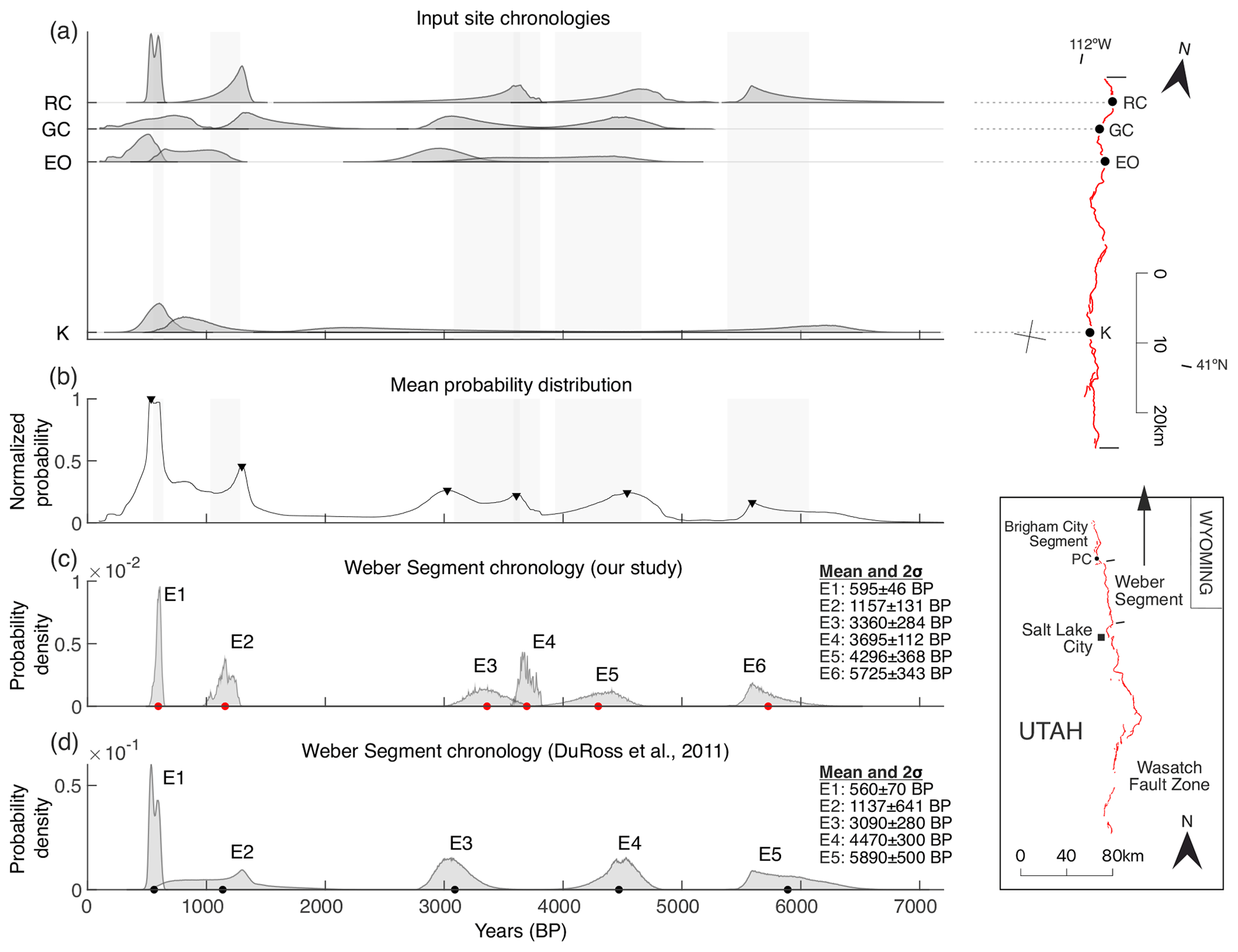
Figure 6 Results of the application of our approach to the Weber Segment of the Wasatch Fault Zone using the OxCal models by DuRoss et al. (2011) at Rice Creek (RC), Garner Canyon (GC), East Ogden (EO), and Kaysville (K). (a) Input site chronologies for all four sites studied. The locations of the sites along the Weber Segment are indicated to the right. The locations of the Weber and Brigham City segments within the Wasatch Fault Zone are indicated in the inset in the lower-right corner of the figure. PC means Pearsons Canyon site. The gray bands indicate the 2σ ranges of the final chronology in panel (c). Fault traces are from the Quaternary Fault and Fold Database of the United States (US Geological Survey and Utah Geological Survey, 2019). (b) Mean distribution resulting from the average of all event PDFs and probability peaks. (c) Final chronology for the Weber Segment with the mean value (dot) indicated for each PDF. (d) Final chronology by DuRoss et al. (2011) computed using the OxCal models provided by these authors in their supplements. Dots indicate the mean value of each PDF. Note that here the timescale is in years BP and event numbers increase for older times to ensure direct comparison with the model by DuRoss et al. (2011).

The above discrepancy in the comparison of our results from the PEACH model with those obtained using the method by DuRoss et al. (2011) suggests the latter may overlook the possibility of paleoseismic underdetection in two scenarios: first, when event PDFs have wide uncertainties, decreasing the confidence that they correspond to a single event; and second, when the PDF skewness might indicate different event occurrences. To tackle this, first, our approach relies on a flexible correlation that allows all events to be correlated with each other if they overlap in time, which, at our criterion, accommodates the geological plausibility of paleoseismic underdetection (i.e., one paleoseismic event representing several events). Second, it uses the shape of the PDFs in the datasets (e.g., peak location and skewness) to determine the number of events in the final chronology. For instance, the added event E4 in our Wasatch Fault chronology comes from the opposing skewness directions of the different PDFs for the events between 2 and 5 kyr BP at the RC and GC sites (Fig. 6c). The statistical confidence of the added event is founded on the characteristics of the PDFs involved in the correlation, namely the geological rationale behind their skewed shapes. As explained by DuRoss et al. (2011), the skewness of the site PDFs in the Weber Segment comes from a forced condition to bias the event ages towards the age of one of the limiting stratigraphic horizons that define the event. This condition is founded on geological observations interpreted by the authors as indicative of the event happening closer in time to one horizon, such as the presence of colluvial wedges or paleosol developments. Based on this reasoning, the opposing skewness of the third PDFs at both RC and GC sites, along with the fact that both events cover a similar time span (Fig. 6), indicates that they likely occurred at different moments in time and therefore could belong to two different events. This two-event interpretation is reinforced by the significant >500-year separation between the higher-probability regions of the mentioned PDFs.

Another difference in the modeling results presented herein from PEACH to those in DuRoss et al. (2011) is that the uncertainties associated with E2 are considerably reduced compared to those estimated by DuRoss et al. (2011) (Fig. 6c and d). That is because, for this event, DuRoss et al. (2011) compute the mean PDF as they debate whether the poor PDF overlap of the penultimate events at all sites would result in overconstraining. However, in the PEACH approach, the product of PDFs constrains the event in the overlapping area of all PDFs, which is where the event is most likely to have happened. Moreover, the shape and uncertainties of the product PDF are comparable to the better-constrained event at that time position (penultimate event at the RC site; Fig. 6a). A mean PDF approach instead of a product one would lead to uncertainty estimates almost as large as the mean (993 ± 747 years BP) and larger than the variance of any of the input event PDFs.

The correlation method by PEACH further allows discussion of fault rupture length and segmentation hypotheses in the Wasatch Fault by using the location of each site chronology along the fault and analyzing the contribution of each event PDF in the chronology (Fig. 6). For instance, the event E4 is mainly defined at the RC site, which means that this event likely ruptured only at that specific location in the Weber Segment. The question is whether the event only ruptured the northern tip of the Weber Segment and is therefore a subsegment rupture or, conversely, corresponds to an inter-segment rupture that jumped across the boundary with the neighboring Brigham Segment to the north. In this line, both scenarios agree with DuRoss et al. (2016) in the sense that partial segment ruptures near or across the primary segment boundaries are regarded as feasible. In detail, they find that E1 at RC in the Weber Segment can be correlated with the youngest and only event recorded at the Pearsons Canyon site (southernmost part of the Brigham Segment; Fig. 6), unveiling a potential inter-segment rupture. Hereby, a similar scenario can be discussed for E4 at RC, although its validation would require the records of both segments to be correlated and analyzed with PEACH, a scope that is beyond this work.

5 Discussion and conclusions

The PEACH approach seeks to maximize the refinement of paleoseismic records using a workflow that relies on a probabilistic modeling of event times from trench numerical dates or pre-computed chronologies from the widely used OxCal software. The approach is flexible and versatile to accommodate several situations of paleodata, e.g., events that cannot be constrained in time individually (site A; Fig. 2e). Moreover, the inputs for the calculations are simple to compile, and the outputs can be easily used to compute fault parameters for the seismic hazard (e.g., average recurrence times and coefficient of variation) in external software programs (e.g., FiSH; Pace et al., 2016).

Our approach is capable of reliably constraining paleoearthquake chronologies from populated records that otherwise would be difficult to correlate manually. The chronologies significantly reduce the uncertainties in the event timing compared to the original data (more than 50 % in the cases exemplified). In addition, the probabilistic treatment of the event times along with a non-restricted site correlation of events seems to perform better in the event detection, allowing an increased total count compared to the trench observations. This can be observed in both cases we exemplify at the Paganica Fault in Central Italy and the Weber Segment in the Wasatch Fault Zone (Figs. 5 and 6) and is a coherent outcome for paleoseismic data, where events evident in trenches are always a minimum relative to the actual number of events that occurred, also considering the wide uncertainties in some of the event dates. Along with this statement, potential cases of event overinterpretation in trenches likely have a reduced impact in our approach. Generally, increasing trench exposures and event correlation across sites reduce the chance of overinterpreting events (e.g., Weldon and Biasi, 2013). That is because true events are likely to be detected at more than one site, as opposed to “fake” or overinterpreted events. In our approach, due to the probabilistic modeling and product-based site-to-site correlations, genuine events tend to stand out more prominently in the mean distribution and have a higher chance of being detected by the algorithm. Conversely, “fake” events are more likely to be downplayed and ruled out of the chronology.

Another strong advantage of our method is that it does not rely on strong expert judgments in the event computation or the correlation. In detail, first, the event PDFs are built considering only the age constraints provided in the input, which should presumably correspond to numerical dates independently dated; i.e., the shape of the event PDF (skewness, width, and height) exclusively depends on the shape of the date PDFs that limit it. Second, the correlation is done independently of the event PDFs involved, meaning that all PDFs that contribute to a peak in the mean distribution, and thus that intersect it, are integrated to compute the final PDF of that event. This removes a layer of expert judgment introduced when correlating only between PDF pairs, like DuRoss et al. (2011), which we suggest could eventually decrease the capability of detecting additional events in the dataset (e.g., smaller events not recorded at all sites).

There are similarities between the PEACH model and the approach previously published in DuRoss et al. (2011). However, herein we suggest that the newer PEACH model performs better in two regards. First, PEACH provides a more objective correlation because we do not pre-impose or condition it to specific PDF pairs. Secondly, the event interpretation performed by PEACH is well adjusted to the event probabilities and shapes of the event PDFs of each site, which are founded on geological observations and criteria from paleoseismologists in the trenches. This interpretation seems to increase the resolution in the event detection by adding one event more while keeping the uncertainties of the event PDFs within acceptable ranges and being overall representative and coherent with the input data.

Besides the advantages, there are limitations in the PEACH approach. Firstly, the use of only a pair of numerical dates to constrain each event PDF can be an oversimplification. This is because some stratigraphic layers can have several dates available with different ages (even inverted stratigraphically) that result from sample-specific anomalies. In radiocarbon, for instance, two samples in the same unit and stratigraphic position can show dissimilar ages due to contamination or carbon inheritance (e.g., Frueh and Lancaster, 2014), especially in the case of snail shells (Goodfriend and Stipp, 1983). The selection of only one date to describe the age of the layer can be inaccurate. Secondly, the assumption of radiocarbon ages shaped as normal distributions is mostly an oversimplification because these usually show irregular or multi-peak shapes due to the calibration. Although such simplification was implemented to accommodate dates from techniques that are expressed as normal distributions (e.g., optically stimulated luminescence), in radiocarbon-dominated datasets the age limits and shape of the resulting event PDFs we compute could be altered, which would ultimately affect the characteristics of the final chronology. In these datasets we recommend pre-computing the site chronologies with OxCal and using the OxCal option in PEACH, not only because of the limitations mentioned in the PDF modeling, but especially because OxCal is designed explicitly for radiocarbon calibration and is therefore better suited to handle the complexities in datasets associated with radiocarbon dating. Having said that, we are committed to improve the code in future updates to allow (i) the introduction of more than one numerical date to define the event time constraints and (ii) complex or multi-peaked radiocarbon PDF shapes.

In terms of event count, our approach strongly relies on the peaks detected in the mean distribution (Figs. 4, 5b, and 6b); i.e., the peak prominence threshold (minprom) has a high impact on the number of peaks that are detected and therefore on the final number of events in the chronology. As the prominence threshold is dependent on the probabilities of the data themselves (Eq. 1) and the final shape of the mean distribution, we cannot ignore the possibility that for some datasets incorrect peak detections could appear. This includes both overdetection and underdetection. The code has several refinements implemented to solve these situations (noisy cluster clearance, sigma truncation, etc.; see Sect. “Refinements of the chronology”), but even when all of them work properly, we strongly recommend the end user to check that the number of events in the final chronology is coherent with the site data. One way to check this could be comparing the event count with the cumulative deformation observed in the trenches, i.e., evaluating whether the number of events is too large or too small to explain the observed deformation. Along this line of reasoning, we clarify that the universality of the approach to all datasets cannot be guaranteed.

With PEACH we highlight how the correlation of paleoseismic datasets with different event completeness degrees and age-constraining quality improves the detection of paleoearthquakes and reduces the uncertainties in event timing. By extension, it can potentially reduce the uncertainties in fault parameter estimates like average recurrence intervals or behavior indicators like the coefficient of variation. Also, the method can be used to explore rupture segmentation behavior through the graphical representations generated during the calculations (e.g., Figs. 5a and 6a), which is to say that the geospatial position of the event site PDFs based on the site location along the fault strike, together with the analysis of the number and timing of events participating in the correlation per site, can give insight into the fault rupture length and fault segmentation. Ultimately these results can be useful to seismic hazard practitioners, as the uncertainties in such parameters are frequent challenges for seismic hazard assessment. For now, we estimate that our method can be reliably used in correlations within the fault level. A measure of the extent of correlation along the fault can come from historical data of surface ruptures. For automatic correlations outside of the fault boundaries (e.g., multi-fault ruptures), further constraints regarding site location and fault distance conditions should be considered and implemented in the code.

We encourage the use of our tool by researchers working on paleoseismology and active tectonics in general, with emphasis on those seeking to improve the time constraints of paleoearthquakes and, additionally, the extent of their surface ruptures along a fault. On top of that, we also invite its users to give the necessary and pertinent feedback to improve our approach in the future.