Representation of atmosphere-induced heterogeneity in land–atmosphere interactions in E3SM–MMFv2

In the Energy Exascale Earth System Model (E3SM) Multi-scale Modeling Framework (MMF), where parameterizations of convection and turbulence are replaced by a 2-D cloud-resolving model (CRM), there are multiple options to represent land–atmosphere interactions. Here, we propose three different coupling strategies, namely the (1) coupling of a single land surface model to the global grid (MMF), (2) coupling a single land copy directly to the embedded CRM (SFLX2CRM), and (3) coupling a single copy of land model to each column of the CRM grid (MAML). In the MAML (Multi-Atmosphere Multi-Land) framework, a land model is coupled to CRM at the CRM-grid scale by coupling an individual copy of a land model to each CRM grid. Therefore, we can represent intra-CRM heterogeneity in the land–atmosphere interaction processes. There are 5-year global simulations run using these three coupling strategies, and we find some regional differences but overall small changes with respect to whether a land model is coupled to CRM or a global atmosphere. In MAML, the spatial heterogeneity within CRM induces stronger turbulence, which leads to the changes in soil moisture, surface heat fluxes, and precipitation. However, the differences in the MAML from the other two cases are rather weak, suggesting that the impact of using MAML does not justify the increase in cost.

1 Introduction

The representation of land–atmosphere interaction processes is important to improve the prediction skills of surface weather and climate in numerical models (Betts, 2004). The key role that land–atmosphere interactions plays in the development of clouds and precipitation is demonstrated in a diurnal timescale (Findell and Eltahir, 2003b, a; Gentine et al., 2013; Vilà-Guerau de Arellano et al., 2014; Guillod et al., 2015) and daily-to-seasonal timescales (Koster, 2010; Hirsch et al., 2014; Dirmeyer and Halder, 2016; Betts et al., 2017). There is also evidence that land–atmosphere interactions can influence the persistence of extreme drought and heat waves (Roundy et al., 2013; Miralles et al., 2014; PaiMazumder and Done, 2016; Wang et al., 2015; Roundy and Santanello, 2017; Dirmeyer et al., 2021).

However, the complexity of land–atmosphere interactions remains a challenge to weather and climate model development. A contributing factor is that the land–atmosphere interaction processes, which strongly control the surface water and energy budget, encompasses a multitude of temporal and spatial scales primarily due to the heterogeneous nature of land surface characteristics (i.e., land cover types, soil types, and terrain). There have been several observational studies to better understand the linkage between the land–atmosphere coupling and its influence on the cloud formation and precipitation processes. However, those study results suggest that the land–atmosphere interaction processes are strongly location-dependent and difficult to generalize (Betts et al., 1996; Betts, 2000, 2004; Ek and Holtslag, 2004; Guo, 2006; Jimenez et al., 2014; Teuling, 2017).

Previously, many numerical studies used a large-eddy simulation (LES) or cloud-resolving model (CRM) with an interactive land surface to better understand the land–atmosphere coupling and its influence on the diurnal cycle of clouds and precipitation (Huang and Margulis, 2009, 2013; Rieck et al., 2014, 2015; Rochetin et al., 2017; Lee et al., 2019). Cloud-resolving scales are more appropriate to resolve the processes that are important to the cloud formation. However, running the global cloud-resolving model is still computationally too expensive to assess the influence of land–atmosphere interaction processes across various temporal and spatial scales.

The Multi-scale Modeling Framework (MMF) approach that is implemented within a global climate model (GCM) can be a good candidate to assess the impact of land–atmosphere coupling on the clouds and precipitation processes. A MMF embeds a fine-scale, cloud-resolving model in each cell of the host model to replace the traditional parameterizations for cloud and turbulence. Therefore, the GCM can explicitly represent convective circulations at a reasonable computational cost. At a resolution on the order of 1 km or shorter, the MMF model can explicitly resolve the key processes for the formation of convective clouds without having to run a global cloud-resolving model (Grabowski, 2004; Khairoutdinov and Randall, 2003; Khairoutdinov et al., 2005).

Traditionally, in the MMF, the land and atmosphere coupling is implemented between the GCM atmosphere and the land model. The CRM embedded inside each GCM grid does not interact directly with the land surface below (Baker et al., 2019). Instead, the GCM interacts directly with the land surface, and these effects are then felt indirectly by the CRM through the tendencies provided by the host GCM. This strategy does not seem to be appropriate, especially when the land–atmosphere coupling plays a key role in the planetary boundary layer (PBL) evolution and convection developments, which are explicitly resolved in the CRM. Therefore, in this study, we propose two different ways to model the coupling directly between CRM and the land model for the MMF configuration of the U.S. Department of Energy's Energy Exascale Earth System Model (E3SMv1; Golaz et al., 2019; Rasch et al., 2019). These two methods differ only by whether the spatial heterogeneity in the land–atmosphere interaction processes is allowed or not. Our approach is based on the single-column model study of representing the heterogeneous land–atmosphere coupling by Baker et al. (2019).

The questions we would like to address in this study are as follows: (1) how does the global climatology change when the land–atmosphere coupling method changes? (2) Are these changes in global climate related to the heterogeneity in land–atmosphere coupling?

The remainder of this paper is organized as follows: Sect. 2 describes the model and the three land–atmosphere coupling strategies in detail. Section 3 documents the simulation results of how different coupling methods influence the cloud formation and land surface evolution. The summary is presented in Sect. 4.

This paper uses several acronyms, and Table A1 is provided in the Appendix to help the reader.

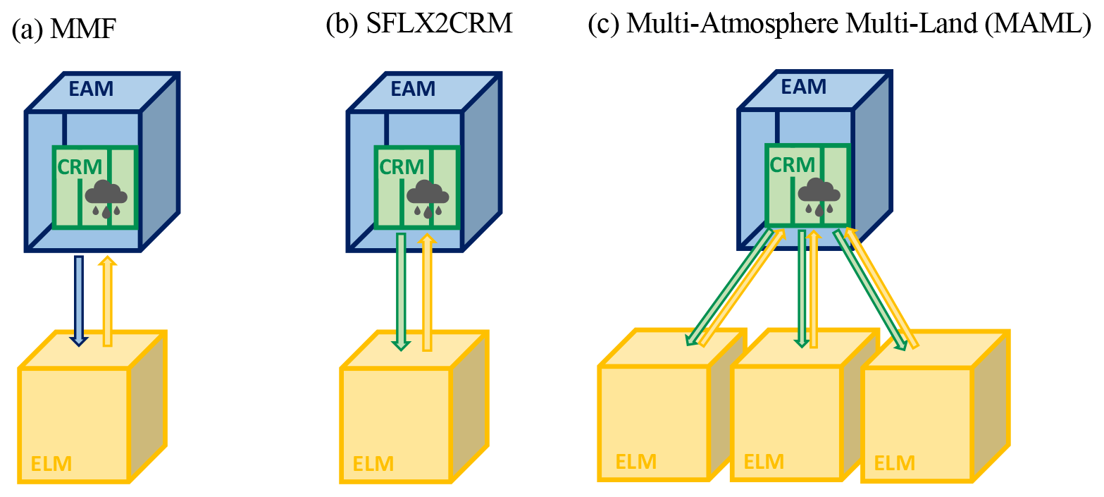
Figure 1 Illustrations of three methods to implement the land–atmosphere coupling in the E3SM–MMF. The blue, green, and yellow boxes represent the EAM (E3SM Atmosphere Model), 2-dimensional CRM atmosphere, and ELM (E3SM Land Model) grid boxes, respectively. The start and end points of each arrow, together with their colors, reflect the interface that is created for the exchange of near-surface meteorological conditions and surface heat fluxes between the land surface and lower-atmospheric boundary layer. In panel (a), the coupling interface is placed between the EAM and ELM, while in panel (b) the interface is put between CRM and ELM. In panel (c), each CRM grid is directly coupled to an independent copy of the land grid.

2 Method

2.1 Model and experiment setup

The model used in this study is the U.S. Department of Energy's Energy Exascale Earth System Model (E3SMv1; Golaz et al., 2019; Rasch et al., 2019) in the Multi-scale Modeling Framework (MMF) configuration. In the MMF approach, a cloud-resolving convective parameterization (i.e., super-parameterization) is integrated into a global atmosphere model. In E3SM–MMFv1, parameterizations for clouds and turbulence in the E3SM Atmosphere Model (EAM) is replaced by a 2-D CRM that is based on the System for Atmospheric Modeling (SAM; Khairoutdinov and Randall, 2003) CRM. The description and performance of the E3SM–MMF is documented in Hannah et al. (2020). The E3SM Land Model (ELM) inherits many of its functionalities from its source model, the Community Land Model, version 4.5 (CLM4.5; Oleson et al., 2013). ELM simulates hydrological and thermal operations in vegetation, snow, and soil for a variety of land cover types, including bare soils, vegetated surfaces, lakes, glaciers, and urban areas. The leaf area index is determined by utilizing satellite data and photosynthesis, without any constraints from leaf nutrients. Since branching off from CLM4.5, ELM has undergone various improvements (Golaz et al., 2019). The impact of aerosol and black carbon on snow was added. The evaporation was reduced over pervious roads under dry conditions. The equation for stomatal conductance was revised to avoid an inaccurate representation of the negative internal leaf CO₂ concentrations. Also, the nighttime albedo over land was updated to 1. In this study, our focus is on exploring various strategies to model the land–atmosphere coupling in the E3SM–MMF and analyze their impact on cloud formation.

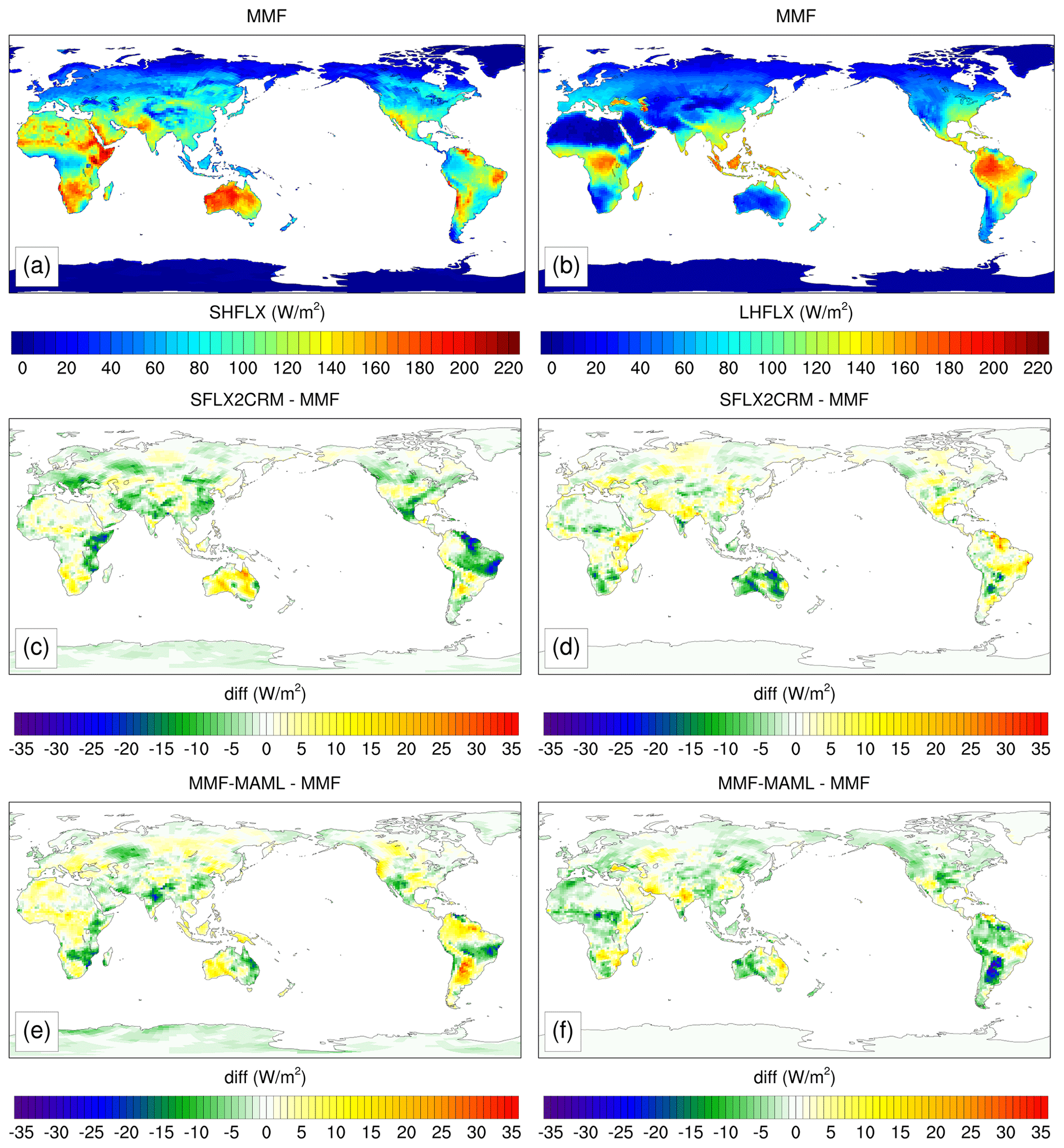
Figure 2 The 5-year averages of daytime (06:00–18:00 local time) mean of the (a, c, e) sensible heat flux (SHFLX) and (b, d, f) latent heat flux (LHFLX) over land only. The top row is from a MMF case, and the remaining two rows are computed by subtracting the MMF from SFLX2CRM and MAML (Multi-Atmosphere Multi-Land), respectively.

We performed three 5-year simulations with E3SM–MMF. The simulations share the same model configuration, except for the land–atmosphere coupling method. The horizontal model grid spacing of the EAM is about 1.5^∘, and the number of vertical model levels is 72, while the model top extends to 60 km. For 2-D CRM, we use 32 columns, with a horizontal grid spacing of 2 km. The CRM time step is 5 s, and the time steps for the EAM physics and ELM (E3SM land model) are 20 min. The sea surface temperature (SST) and aerosol concentrations are prescribed using the climatology across the 10-year period and centered at year 2000. A one-moment microphysics scheme is used inside the CRM to compute clouds and precipitation processes. The Smagorinsky scheme is responsible for parameterizing the sub-grid-scale turbulence in the CRM. Since we use a 2-D CRM, the meridional component of the wind can be too strong; therefore, this misleads the land surface processes if CRM wind fields are coupled to the ELM. To bypass this difficulty, we use the wind velocities from EAM in all three methods. There is also a time step difference between ELM and CRM, as CRM subcycles with a much shorter timescale (dt) within a single time step of the EAM (dT). EAM and ELM share the same time step. Therefore, the CRM states that are passed to ELM are temporally averaged over dT at the end of the subcycling, and the land surface states do not change, while the CRM subcycles. The land model's initial conditions are spun-up, using 20 years of National Centers for Environmental Prediction (NCEP) reanalysis data. For the radiation scheme, we used RRTMGP (Pincus et al., 2019). To decrease the computational cost, we used a method with which a certain number of CRM columns is grouped together for the radiation calculations. In our study, we grouped two neighboring CRM columns to compute radiation instead of computing the radiation in each CRM grid.

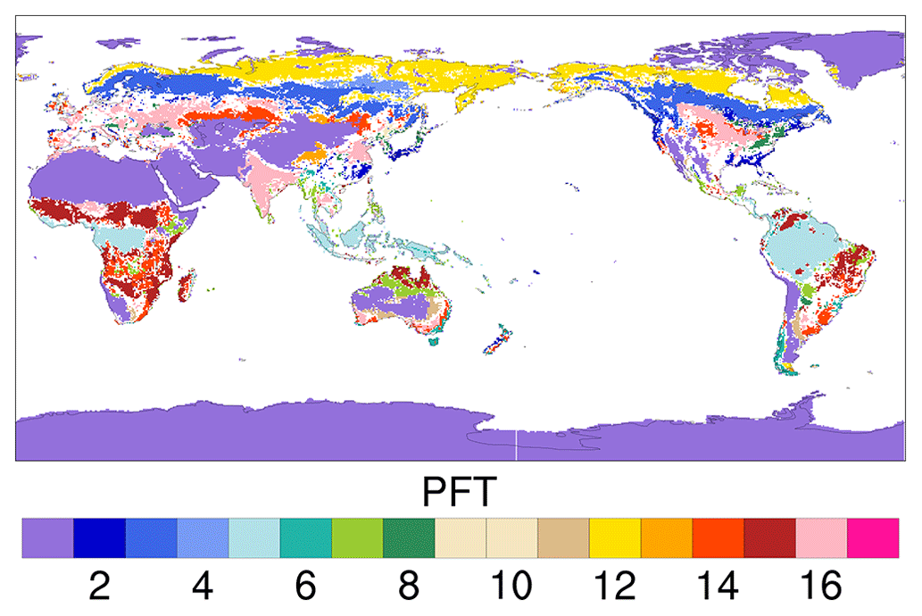
Figure 3 Global map of plant functional types (PFTs) that cover more than 50 % of each land unit grid cell in ELM. The vegetation types that each PFT number indicates are as follows: 1 for bare soil, 2 for needleleaf evergreen temperate, 3 for needleleaf evergreen boreal, 4 for needleleaf deciduous boreal, 5 for broadleaf evergreen tropical, 6 for broadleaf evergreen temperature, 7 for broadleaf deciduous tropical, 8 for broadleaf deciduous temperate, 9 for broadleaf deciduous boreal, 10 for broadleaf evergreen temperate shrub, 11 for broadleaf deciduous temperate shrub, 12 for broadleaf deciduous boreal shrub, 13 for arctic C3 grass, 14 for cool C3 grass, 15 for warm C4 grass, and 16 for crops.

2.2 The land–atmosphere coupling strategies for the E3SM–MMF

The coupling between the land and atmosphere models is implemented as the exchange of near-surface atmospheric states and land surface energy fluxes. The near-surface meteorological conditions include downwelling radiative fluxes, temperature, moisture, wind speed, and precipitation rate from the lowest model level. The land surface fields that are used as atmospheric lower-boundary conditions include surface latent and sensible heat fluxes and land surface temperature. Also, upwelling short- and long-wave radiative fluxes are returned from the land model to the atmosphere's radiation scheme. In this study, we explore three strategies to implement the coupled exchange of water and energy between an atmosphere and a land surface in the E3SM–MMF, where the complexity increases as numerical simulations of an atmosphere are performed both in the EAM and CRM components.

The default method to couple the land and atmosphere models is to exchange fluxes directly between EAM and ELM and use the modified EAM state to force the embedded CRM, as shown in Fig. 1a. Therefore, the CRM experiences the effect of land surface energy fluxes indirectly through the large-scale forcing given by the EAM. This method allows for both atmosphere and land physics to be updated at the same timescale. E3SM and original version of the E3SM–MMF adopt this strategy. This method is labeled as “MMF” throughout this study.

Table 1 The 5-year global means over land for MMF, SFLX2CRM, and MAML cases. SHFLX is sensible heat flux, and LHFLX is latent heat flux. SOILWATER_10CM is top 10 cm integrated soil moisture, and TSOIL_10CM is soil temperature for top 10 cm depth. FCEV is direct evaporation from vegetation moisture. FCTR is vegetation transpiration. FGEV is soil evaporation. PRECT is the surface rainfall rate.

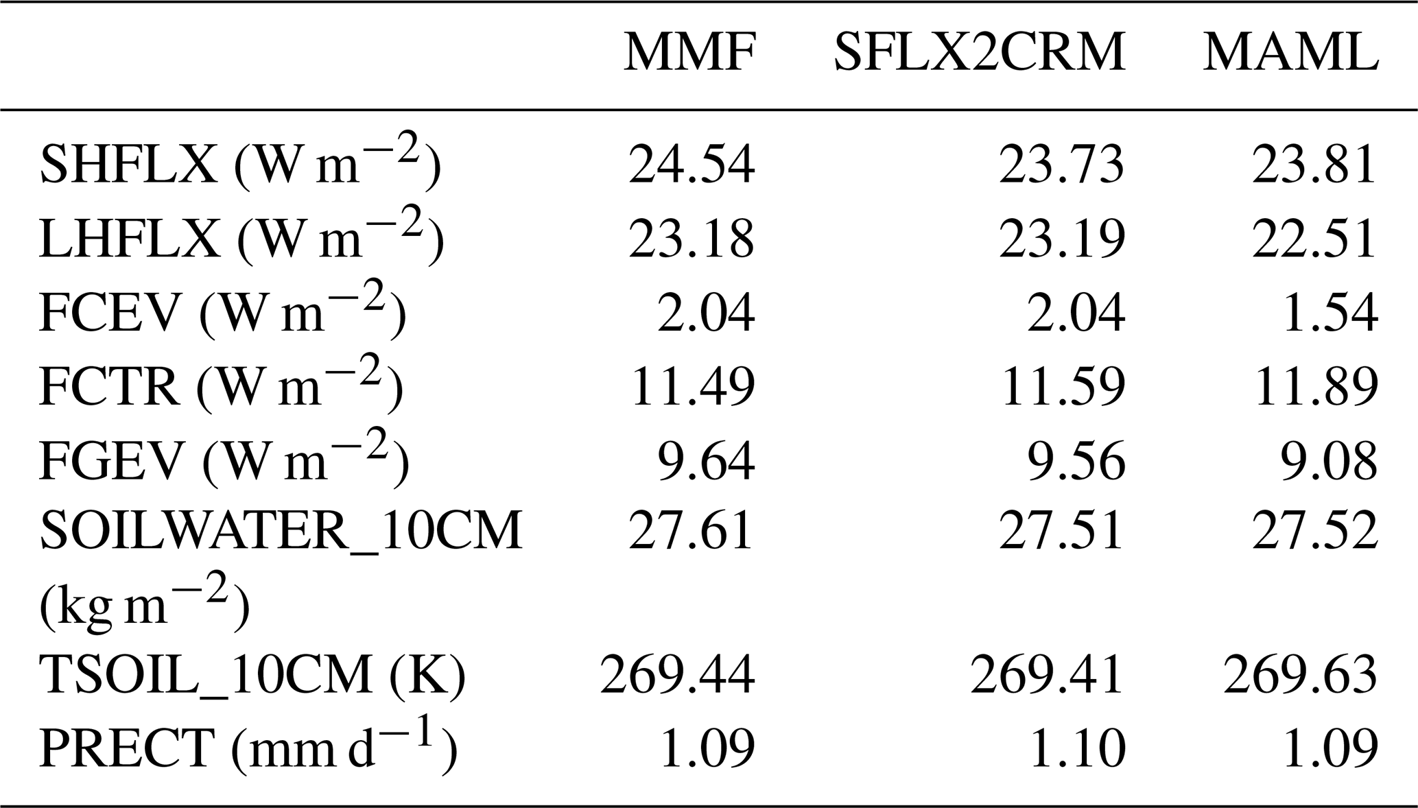
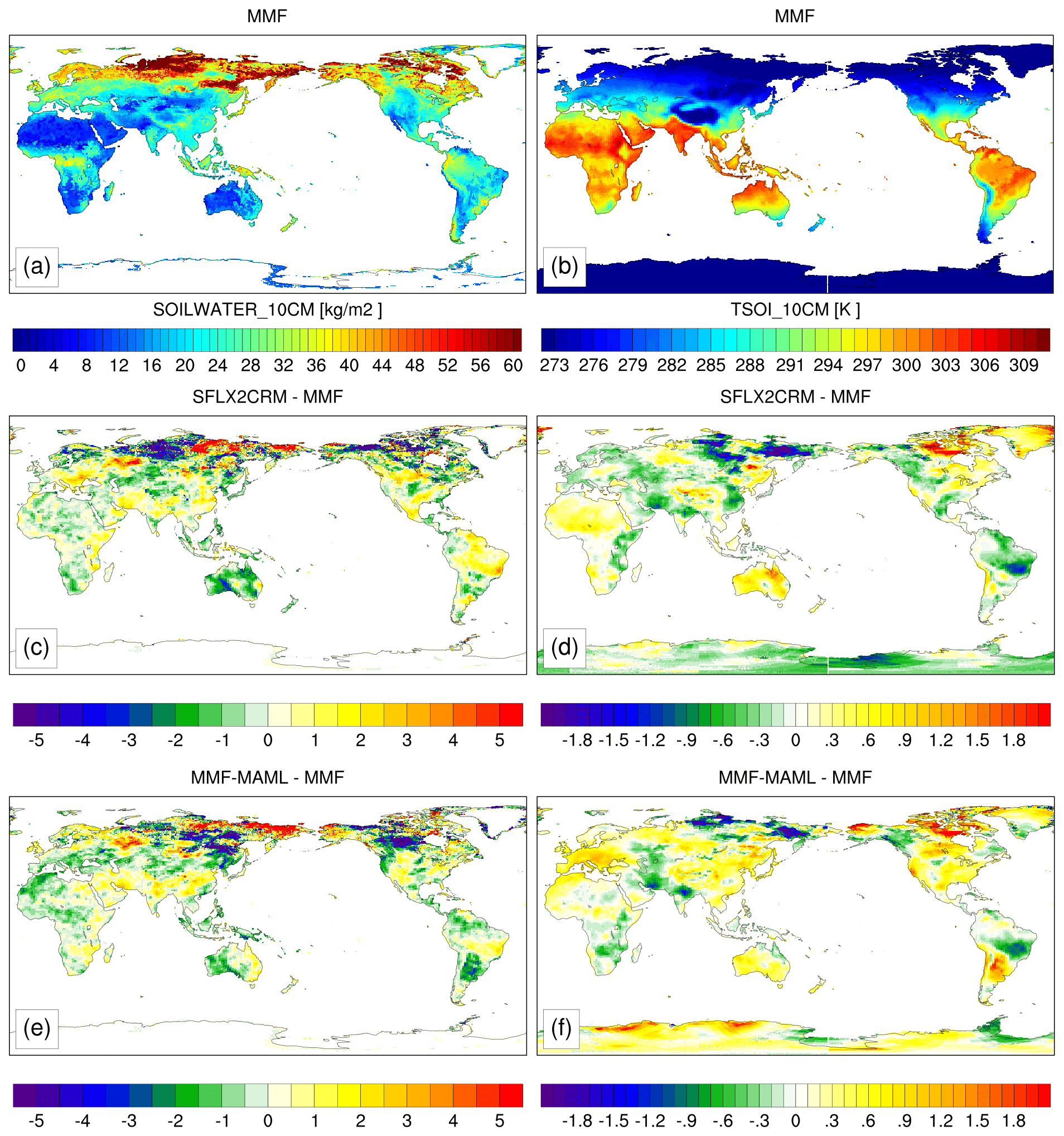
Figure 4 The 5-year annual climatologies of the (a, c, e) top 10 cm soil moisture (SOILWATER_10CM) and (b, d, f) top 10 cm soil temperature (TSOI_10CM). The top row is from the MMF case, and the remaining two rows are computed by subtracting MMF from SFLX2CRM and MAML, respectively.

Another method is presented in Fig. 1b, showing where a set of near-surface meteorological conditions and a set of land surface energy fluxes are exchanged between the CRM and the ELM. The near-surface meteorological conditions are averaged across the CRM domain, and these spatially averaged fields serve as an input to the ELM. The surface heat fluxes computed by the ELM are applied homogeneously as a bottom boundary condition across the CRM domain. This method prescribes surface buoyancy forcing that is horizontally homogeneous. This method is called “SFLX2CRM” hereafter.

The third method is based on SFLX2CRM and allows spatial heterogeneity across the CRM domain by associating each CRM column with a separate copy of ELM. This approach is made possible by the multi-instance functionality of the E3SM, which was originally developed to perform ensemble simulations. For instance, when the CRM is used with nx (number of horizontal grids) horizontal grids, we set up the model to run nx copies of ELM. The coupling is done at the interface between the CRM and the ELM, where each CRM grid is coupled to an independent copy of ELM but on the timescale of the EAM time step. This is where the name Multi-Atmosphere Multi-Land (MAML) comes from. These nx copies of ELM feature the same land surface characteristics. Also, CRM does not include CRM-scale topography. Therefore, this method does not fully represent a significant level of surface heterogeneity. Using EAM wind to drive land surface processes and grouping neighboring CRM columns for radiation calculation decreases the heterogeneity induced by atmosphere in MAML. We did not test how these modifications would affect the resulting climate.

SFLX2CRM and MAML were previously introduced in Baker et al. (2019) for different atmosphere and land models. Baker et al. (2019) ran single-column model simulations of the MMF model, with changes in terms of how the models couple to land surface for the Brazilian Forest, while our study runs global simulations to assess the influence of heterogeneous land–atmosphere interaction processes on the global climate. Lin et al. (2023) also presented a method for surface–atmosphere coupling at cloud-resolving scale within the MMF configuration of E3SMv1. Lin et al. (2023) uses the terminology of MAML for the framework in which the land states are averaged across the land copies before being coupled to the CRM columns. It is important to acknowledge that the Lin et al. (2023) MAML is different to our MAML method.

The cases in this study are referred to as MMF, SFLX2CRM, or MAML, following the strategies introduced in Fig. 1. The influence of land–atmosphere coupling on the simulated climate is analyzed over land only for the entire 5-year simulation period.

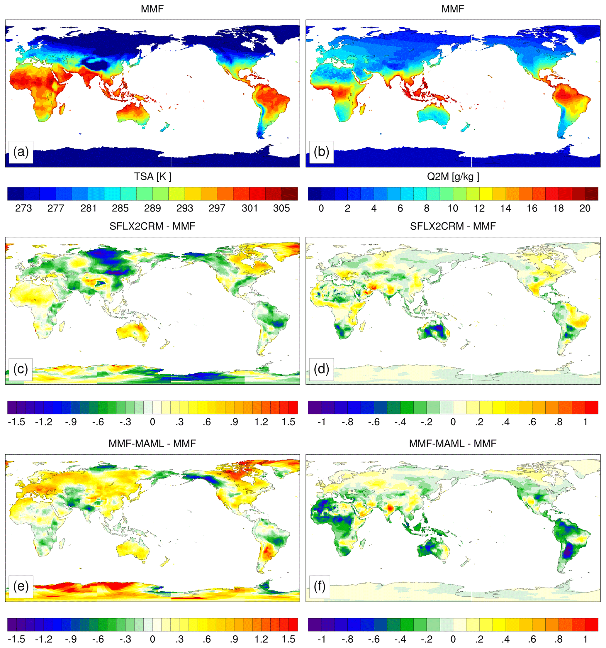
Figure 5 The 5-year annual climatologies of (a, c, e) 2 m surface air temperature (TSA) and (b, d, f) 2 m specific humidity (Q2M). The top row is from a MMF case, and the middle two rows are the changes in SFLX2CRM and MAML from the MMF simulation.

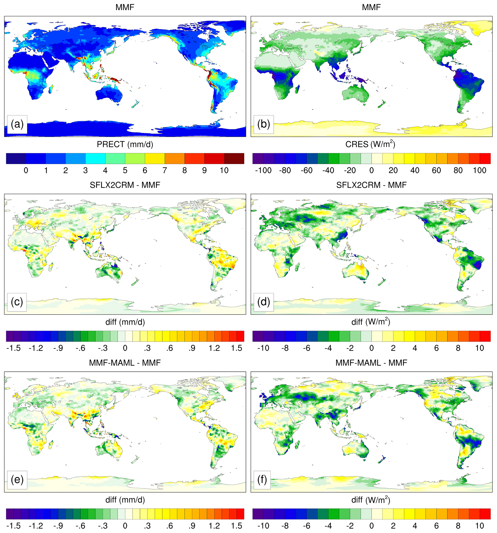
Figure 6 Same as Fig. 5 but for the (a, c, e) surface rainfall rate (PRECT) and (b, d, f) net cloud radiative effect at surface (CRES).

3 Results

3.1 Climatology overview

Figure 2 a and b show the annual mean of daytime surface sensible (SHFLX; left column) and latent heat fluxes (LHFLX; right column) of the MMF simulation. Surface sensible heat fluxes over land experience a strong diurnal cycle, which reaches maximum around local noon. Therefore, only daytime values, which cover the period from 6:00 to 18:00 local time, were averaged to emphasize the differences between simulations. In comparison to the 5-year climatology, the magnitudes of the daytime mean fluxes are higher than the number of annual mean fluxes, and spatial patterns of fluxes remain the same (not shown). However, one should note that the day length in the extra-tropics is shorter in wintertime.

Spatial distributions of surface sensible and latent heat fluxes show a strong dependency on the land cover types. Figure 3 is a global map of the prescribed plant functional types (PFTs) that are dominant for each land unit in ELM. The dominant PFT is determined by any PFT of which the coverage for each land unit is greater than 50 %. The areas in which there is no dominant PFT, such as boundaries of vegetation type changes or highly heterogeneous areas, are marked white. It is notable that the evaporation in Fig. 2b is the strongest in the tropical and sub-tropical regions, where the primary vegetation types are broadleaf evergreen tropical (PFT = 5), broadleaf deciduous tropical (7), cool C3 grass (14), warm C4 grass (15), and crops (16). On the other hand, regions in the tropics and the sub-tropics with no vegetation cover (1) produce stronger sensible heating, as shown in Fig. 2a.

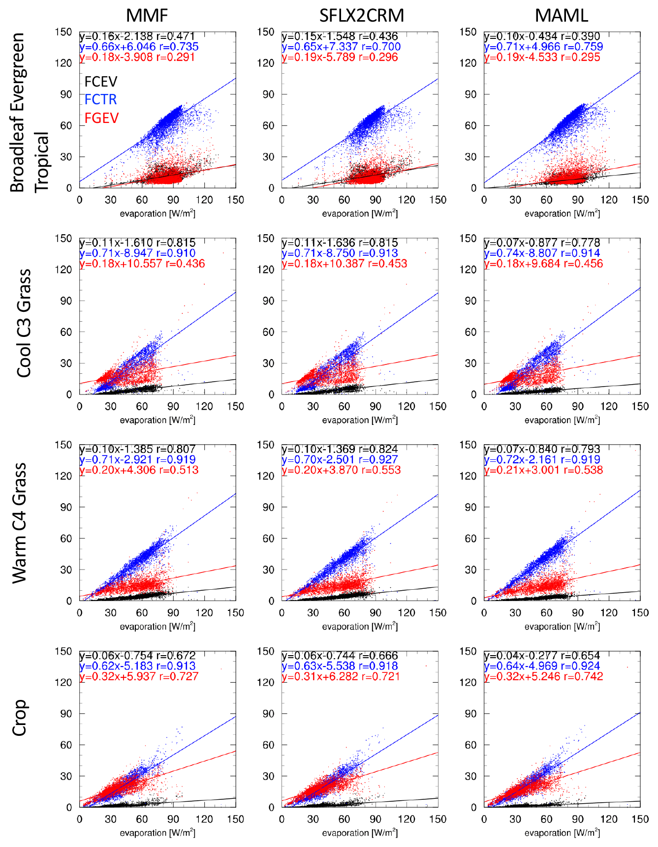
Figure 7 Scatterplots of total evaporation (x axis) and its components (y axis), with the (black; FCEV) direct evaporation rate from the moisture intercepted by vegetation; (blue; FCTR) evaporation rate from vegetation transpiration, and (red; FGEV) evaporation rate from the soil surface against total evaporation. Each column represents different cases, including (left) MMF, (center) SFLX2CRM, and (right) MAML. Each row denotes a different vegetation by PFT type. The equations denote the slope and y intercept of a given linear regression line.

Figure 4a and b show 5-year means of soil moisture (SOILWATER_10CM) and temperature (TSOI_10CM) of the MMF simulation. In general, the MMF case shows that areas with high soil saturation level and low soil temperature and high evaporative fraction (EF = LHF/(SHF+LHF)), such as the Amazon Basin, eastern USA, tropical Africa, and the Maritime Continent, overlap with the regions with high surface evaporation, whereas areas with arid climate, such as Australia and deserts in Africa, commonly show a low soil saturation level, high soil temperature, and low evaporative fraction. As shown in Fig. 3, among the vegetated regions, areas covered with shorter and less dense vegetation types, such as grass and crops, exhibit higher soil temperature in comparison to the areas with dense forest. Figure 5a and b show annual means of near-surface temperature (TSA) and specific humidity (Q2M) from the MMF. The response of surface heat fluxes to the near-surface atmospheric temperature and moisture quantity presents a few important features. Similar to the relationship between soil moisture and temperature with surface heat fluxes, the near-surface atmosphere also shows a dependency on the evaporative fraction. The regions where the evaporative fraction is low, i.e., where the sensible heat flux is higher than the evaporation, have a high atmospheric temperature and low moisture content. Therefore, the relative humidity (RH) is low over areas such as northern and southern Africa and Australia, which also overlaps with the descending Hadley circulation. On the other hand, the tropical rainforest regions exhibit higher relative humidity in response to the higher latent heat flux. Figure 6a shows that the climatological precipitation over land tends to favor the areas with high atmospheric humidity. Even in the Amazon Basin, where both large-scale circulation from terrain and local-scale land–atmosphere interaction processes are significant, we see that the location of the enhanced precipitation grossly follows the areas of high evaporation and high soil moisture level. Figure 6b shows the net cloud radiative effect at surface (CRES) that is determined by summing the differences in downwelling longwave radiation between clear-sky and cloudy-sky conditions and in downwelling shortwave radiation between clear-sky and cloudy-sky conditions. The surface net cloud radiative effect that has a cooling effect indicates the presence of liquid clouds, as they reflect more solar radiation than absorbing terrestrial infrared radiation (IR). The spatial distribution of clouds overlaps well with the location of precipitation over land, which also has a strong dependency on the location of the wet soil. Therefore, our MMF case shows that regions of high precipitation overlap the areas with wet soil, especially in a tropical belt.

3.2 Influences of heterogeneous land–atmosphere interaction on global climate

Global means that are computed over land only suggest that the differences between each case are small (Table 1). The response of surface energy and water cycle to the land–atmosphere coupling in E3SM–MMF is shown in terms of the changes in SFLX2CRM and MAML from the MMF simulation. As shown in Fig. 1 through 6 (except for Fig. 3), when the land model is directly coupled with CRM (SFLX2CRM and MAML), we see many small differences but no systematic change that is consistent across different regions. Notable differences tend to be co-located with the areas of high net surface radiation, which is approximately equal to the sum of sensible and latent heat fluxes (i.e., tropical–subtropical band). For example, precipitation and cloud radiative effect at surface shows noticeable differences in SFLX2CRM and MAML over the Amazon, North America, eastern Asia, and central Africa regions.

For a given net surface radiation at each grid cells, the increase in the surface evaporation leads to the reduction in sensible heat flux (Fig. 2). While changes in SFLX2CRM are small, MAML shows an appreciable reduction in the latent heat flux (therefore, an increase in the sensible heat flux) over the tropical rainforest regions. In comparison to the MMF, a global mean of land evaporation in SFLX2CRM changes by 0.08 % (0.02 W m⁻²), while the change is −2.9 % (−0.6 W m⁻²) in MAML (Table 1). The total evaporation from the land surface is composed of (1) direct evaporation from the water present on vegetation surface, (2) transpiration, and (3) evaporation from soil top. Figure 7 shows ratios of each evaporation component to the total evaporation for each grid cell from the 5-year annual mean. The left column is the relationship for the MMF case, while the other two columns are from SFLX2CRM and MAML cases, respectively. For each row, the relationship is shown for different PFT types. Each row represents the relationship for the broadleaf evergreen tropical type (PFT = 5), cool C3 grass (14), warm C4 grass (15), and crops (16), respectively. These four PFT types cover the largest area globally and are mostly found in the tropics–subtropics belt.

In Fig. 7, the fact that the vegetation transpiration makes up most of the total evaporation into the atmosphere regardless of vegetation types stands out. The ratio of transpiration to the total evaporation is the highest for broadleaf evergreen tropical type. Direct evaporation from vegetation in SFLX2CRM shows an insignificant change relative to the MMF case, while the same field in the MAML case decreases overall by 33 % (3.8 W m⁻²). The source of moisture present on the vegetation surface is dependent on rainfall and nighttime dew formation. The fact that MAML shows a reduction in the direct evaporation from vegetation could be related to the decrease in rainfall and increase in temperature, which could prevent dew formation. In addition, MAML indicates an increase in the transpiration approximately 1.31 W m⁻² in the tropical regions in Africa and South America, despite a slight reduction in the soil moisture in comparison to the other two cases. This feature also suggests that land–atmosphere coupling via MAML method increases surface temperature; therefore, the vapor deficit at the vegetation layer level worsens, which leads to the higher potential for transpiration. Since the transpiration of a rainforest withdraws soil moisture in the root zone, there was less impact by near-surface soil moisture. For tropical rainforest regions, the reduction in the latent heat flux in MAML is due to the reduction in the direct evaporation of moisture stored on vegetation surfaces.

In comparison to tropical evergreen broadleaf trees, C3 and C4 grasses and crops are shorter and have a lower leaf area index. These phenology makes grasses and crop types are more sensitive to the soil moisture when determining the total evaporation into the atmosphere. In fact, the ratio of soil evaporation to the total increases for grasses and crop types. The most dominant land type in India is crops and fields, as shown in Fig. 3. MAML has increased soil moisture over India (Fig. 4e), which results in the increased transpiration and soil evaporation. Similarly, C3 and C4 grass-covered areas also show a strong dependency on the soil moisture. For instance, the northern side of the Democratic Republic of the Congo (DRC) experiences reduced soil moisture and therefore a decrease in surface evaporation, while the southern side of the DRC exhibits increased soil moisture and therefore an increase in surface evaporation. Figure 5 shows how the lower-atmosphere meteorological condition is influenced by below-surface heat fluxes and soil moisture. Regions with higher (lower) evaporation align with regions with a humid (dry) PBL. Comparison with Fig. 6 confirms that precipitation is favorable over the regions where the PBL is humid. Figure 8 shows scatterplots for each segment of soil moisture–PBL–precipitation interactions. These scatterplots show that a positive correlation exists between the soil moisture and evaporative fraction (EF), the EF and near-surface humidity, and the near-surface humidity and precipitation. There are no noticeable differences between each case. As suggested before, coupling a CRM and land model affects the PBL thermodynamics and therefore affects cloud processes that are triggered by PBL turbulence. However, the MAML case demonstrates that the land–atmosphere interactions are at CRM-grid scales and that the spatial heterogeneity within each CRM domain contributes to warmer and drier PBL; therefore, there are fewer liquid clouds and less precipitation over land.

3.3 Spatial heterogeneity within CRM column

The states of land and atmosphere experience stronger adjustments when the CRM is coupled with land, and these adjustments are enhanced when the spatial heterogeneity of the coupling inside the CRM is allowed in MAML. Figure 9 shows the normalized standard deviation of surface heat fluxes, soil temperature, soil moisture content, 2 m atmospheric humidity, and precipitation across 32 land model copies. We use the standard deviation as a measure of the CRM-scale spatial heterogeneity (Fig. 9). Strong spatial heterogeneity in land surface processes is found where the MAML differs from the MMF the most by visually inspecting Figs. 2 and 4–6. Therefore, where the differences between MMF and MAML are the largest in the land surface states, precipitation roughly overlaps with the areas with a strong standard deviation. Therefore, the stronger global mean deviation in the MAML can be attributable to the spatial heterogeneity in land–atmosphere interactions.

However, the spatial heterogeneity in the lower atmosphere in terms of the temperature and moisture seems to be insignificant in comparison to that in the land states. This is due to the mixing inside the CRM that homogenizes the atmosphere, while such horizontal mixing processes are missing within 32 ELM copies. This could explain the little changes induced by the MAML land–atmosphere coupling method.

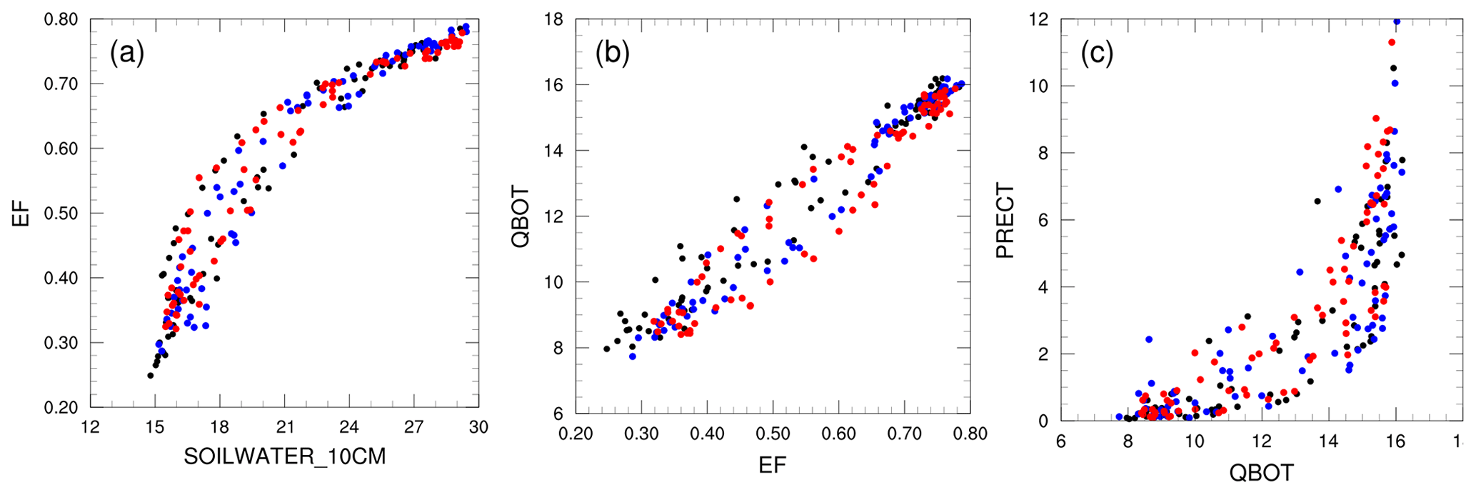
Figure 8 Scatterplots of 5 d averages of (a) near-surface soil moisture versus evaporative fraction, (b) evaporative fraction versus near-surface specific humidity, and (c) near-surface specific humidity versus precipitation averaged over Amazon. MMF, SFLX2CRM, and MAML are denoted by black, blue, and red dots, respectively.

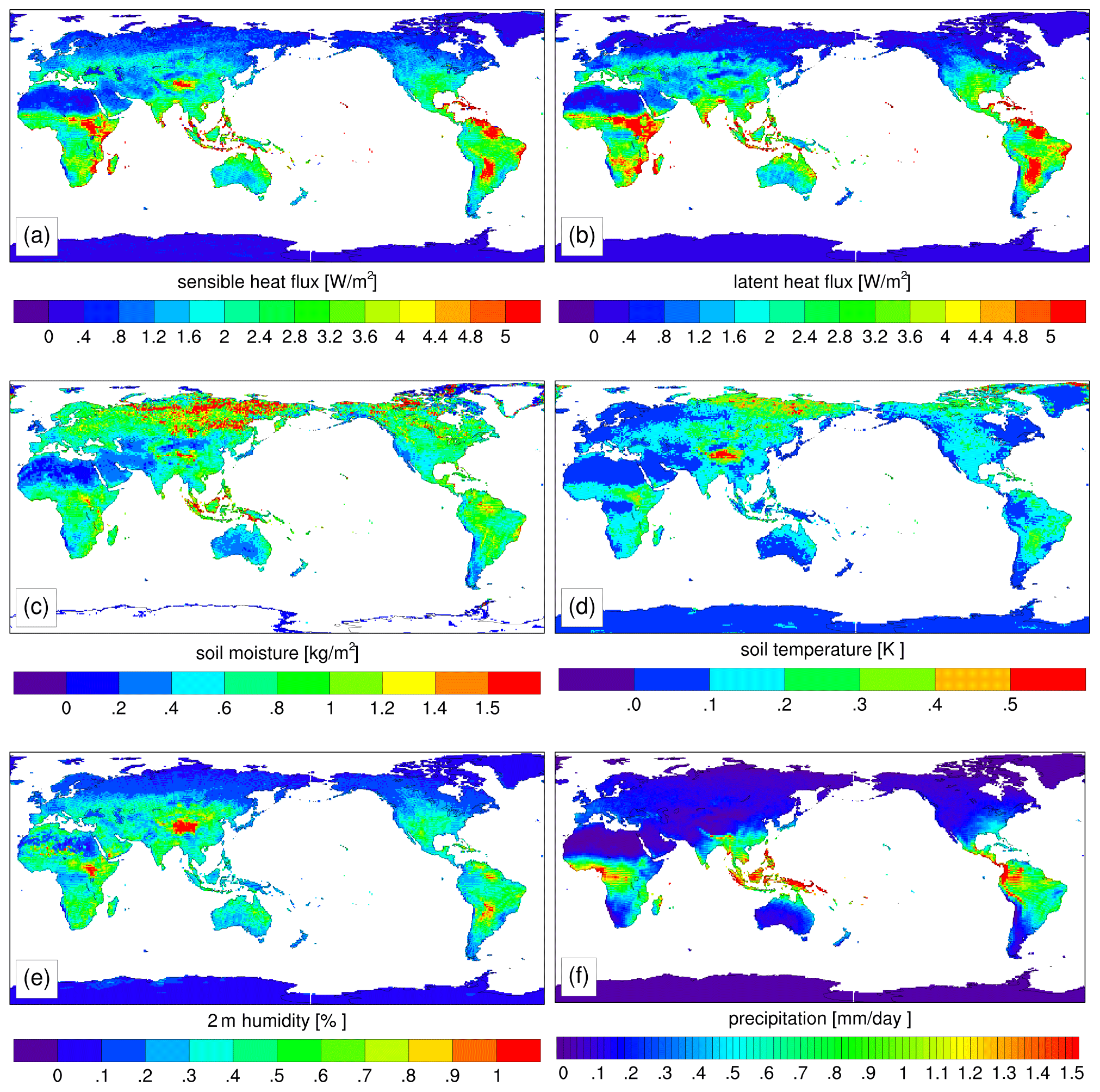
Figure 9 Standard deviation of 5-year climatology of (a) sensible heat flux, (b) latent heat flux, (c) top 10 cm soil moisture, (d) top 10 cm soil temperature, (e) lower-atmosphere relative humidity, and (f) surface precipitation across 32 land copies.

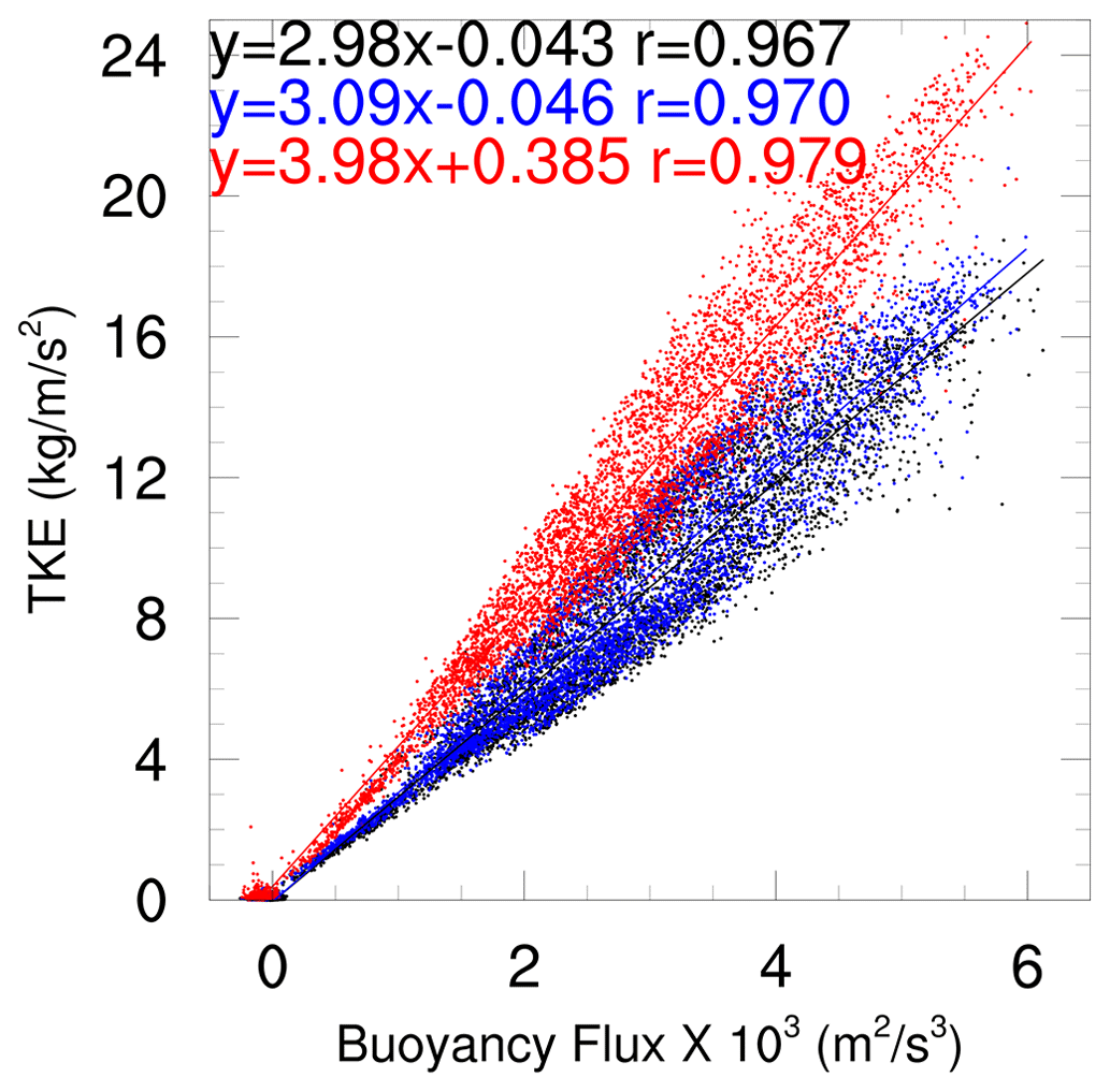
Figure 10 Scatterplot of surface buoyancy flux and lowest model-level turbulence kinetic energy (TKE), with a fitted linear regression line for each case. Each dot represents an annual mean of the daytime mean (06:00–18:00 local time) of a single model grid over land. Each case is drawn in a different color. MMF, SFLX2CRM, and MAML are marked in black, blue, and red dots, respectively. The linear regression equation and the correlation coefficient R are written in a color matching that of each case.

3.4 Stronger PBL turbulence in MAML

Figure 10 shows the scatterplot between surface buoyancy flux in x axis and production of TKE in the y axis. Surface buoyancy flux (BFLX) is diagnosed inside the code as

$$\begin{array}{}\text{(1)}& \mathrm{BFLX}={\displaystyle \frac{\mathrm{SHF}}{c_{\mathrm{p}}}}+\mathrm{0.61}{T}_{\mathrm{s}}{\displaystyle \frac{\mathrm{LHF}}{L_{\mathrm{v}}}},\end{array}$$

where SHF (LHF) is sensible (latent) heat flux, c_p is the specific heat of the air, T_s is the near-surface temperature, and L_v is latent heat of vaporization. For the MAML case, BFLX is computed for each land model copy. Each dot in Fig. 10 represents a 5-year mean of daytime (06:00–18:00 local time) mean values for a given land grid point. Figure 10 shows that there is a linearly positive relationship between the surface buoyancy flux and TKE. Therefore, it is shown that a stronger buoyancy flux at the surface results in stronger TKE in all cases. All land points show a stronger TKE in MAML for a given buoyancy flux, while there is little difference between MMF and SFLX2CRM. This is due to the fact that in SFLX2CRM, the ELM computes the buoyancy flux based on the homogeneous meteorological condition within a CRM, which is similar to that of the MMF. On the other hand, in MAML, the heterogeneity in the surface buoyancy fluxes contributes to the stronger PBL turbulence.

Figure 11 presents a globally averaged profile of the TKE and liquid cloud water content over land. In MMF, excessive condensation in the lowest model level over land is a globally common feature, as shown in Fig. 11. Gettelman et al. (2020) reported that CAM5 also develops clouds in the lowest-model-level layer (“stratofogulus”) because the boundary layer circulation is inefficient for transporting water vapor from the near-surface to higher levels. However, the model with CRM with an interactive land surface (SFLX2CRM and MAML) shows a significant reduction in such cloud formation in the lowest model level. This is due to the PBL turbulence triggered by the surface buoyancy that is effectively transporting the near-surface air mass vertically. This process, unlike SFLX2CRM and MAML, where CRM is coupled to ELM, was missing when EAM had an interactive land surface (MMF), as these turbulent transport processes in response to the land surface heating were not adequately resolved. In MMF, CRM does not receive surface heat fluxes from ELM and therefore computes TKE based on the thermodynamic profile. Since MMF and SFLX2CRM have a similar thermodynamic profile, both produce a similar TKE profile. However, near the surface, SFLX2CRM has slightly higher TKE due to the non-zero surface buoyancy flux. This is the reason why there is a large difference in the liquid cloud water profile when the TKE is similar. TKE in MAML is stronger than SFLX2CRM (Fig. 10), which explains the further reduction in the condensation at the model level.

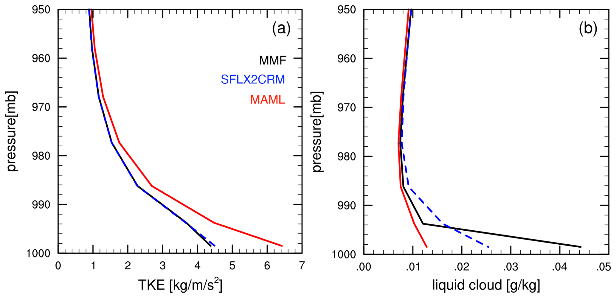
Figure 11 Globally (land-only) averaged vertical profile of (a) turbulent kinetic energy (TKE) and (b) liquid cloud moisture content. MMF, SFLX2CRM, and MAML are marked in different colors using black, blue, and red, respectively.

4 Conclusions

Here, we present a numerical study that explores three methods to model the local-scale land–atmosphere interaction processes in the MMF version of E3SM. Traditionally, in Earth system models, an atmosphere and a land are coupled at each large-scale grid, which is generally of the order of 100 km. Land surfaces are characterized by land cover, terrain, and soil texture, which are naturally heterogeneous across various spatiotemporal scales. Therefore, a coupling scale that is too large between land and atmosphere can easily undermine the importance of land–atmosphere interactions and their impact on convective cloud formations. The MMF allows a global atmospheric model to run at a cloud-resolving scale, which gives us a motivation to explore the impact of coupling land–atmosphere at cloud-resolving scales on the energy and water budget at land surface. Alongside the traditional method of coupling land–atmosphere in E3SM, two strategies are assessed at the global scale from Baker et al. (2019), both using a 2-D CRM with an interactive land surface. Therefore, these two methods can exchange energy and water directly between CRM and a land model. The first method exchanges CRM-domain-averaged values with a single copy of the land model; therefore, only homogeneous interactions are allowed (SFLX2CRM). The second method allows an intra-CRM heterogeneity by coupling each CRM grid with its own land model. In our study, we used a 2-D CRM with 32 grid points, and each of these 32 CRM columns has its own land surface (MAML). By analyzing the 5-year model output, we see that the model simulation demonstrates the positive feedback between soil moisture, evaporation, PBL humidity, and precipitation, as stronger precipitation is observed over the areas with higher soil moisture. We find that the global means of SFLX2CRM are similar to that of MMF. However, MAML tends to produce drier and warmer surface weather. In MAML, the warmer temperature increases the transpiration of the rainforest, while there is an insignificant change in the direct soil evaporation. However, the evaporation of the moisture stored on vegetation surfaces decreases, and this reduction overpowers the increase in the transpiration. On the other hand, for C3 and C4 grasses and crops and/or fields tend to be more sensitive to the soil moisture when determining the total evaporation. As the MAML simulation produces lower soil moisture, the total evaporation over grasses and crops and/or fields also decreases. Therefore, the total evaporation is reduced, regardless of vegetation type, in MAML in comparison to MMF and SFLX2CRM. A future study can do a follow-up investigation on the sensitivity of precipitation to the soil moisture in E3SM–MMF.

The current model configuration of the MAML framework, where each land copy is configured with the same land surface characteristics, produces a heterogeneity in land–atmosphere interactions that is too weak. Therefore, we do not see any drastic changes in the precipitation and cloud formation. However, this work provides a modeling framework in which MAML can be used an advanced modeling tool. In this framework, it is simple to prescribe each ELM copy with different land surface characteristics. However, it is non-trivial to prescribe realistic heterogeneity in land surface characteristics for a 2-D modeling space. Therefore, an additional study can help us to investigate the role of the truly heterogeneous land surface characteristics in land–atmosphere interactions in a global-scale model.

Appendix A: Table of acronyms

Acronym	Meaning
BFLX	Surface buoyancy flux
CRES	Net cloud radiative effect at surface
CRM	Cloud-resolving model
EAM	E3SM Atmosphere Model
EF	Evaporative fraction
ELM	E3SM Land Model
E3SM	Energy Exascale Earth System Model
GCM	Global climate model
LHFLX	Latent heat flux
MMF	Multi-scale Modeling Framework
PBL	Planetary boundary layer
PFT	Plant functional type
Q2M	Specific humidity at 2 m height
RH	Relative humidity
SAM	System for Atmospheric Modeling
SHFLX	Sensible heat flux
SST	Sea surface temperature
TKE	Turbulence kinetic energy
TSA	Temperature at 2 m height
TSOI_10CM	Soil temperature in the upper 10 cm