Calibration of absorbing boundary layers for geoacoustic wave modeling in pseudo-spectral time-domain methods

This paper develops a calibration methodology of the artificial absorbing techniques typically used by Fourier pseudo-spectral time-domain (PSTD) methods for geoacoustic wave simulations. Specifically, we consider the damped wave equation (DWE) that results from adding a dissipation term to the original wave equation, the sponge boundary layer (SBL) that applies an exponentially decaying factor directly to the wavefields, and finally, a classical split formulation of the perfectly matched layer (PML). These three techniques belong to the same family of absorbing boundary layers (ABLs), where outgoing waves and edge reflections are progressively damped across a grid zone of N_ABL consecutive layers. The ABLs used are compatible with a pure Fourier formulation of PSTD. We first characterize the three ABLs with respect to multiple sets of N_ABL and their respective absorption parameters for homogeneous media. Next, we validate our findings in heterogeneous media of increasing complexity, starting with a layered medium and finishing with the SEG/EAGE 3D salt model. Finally, we algorithmically compare the three PSTD–ABL methods in terms of memory demands and computational cost. An interesting result is that PML, despite outperforming the absorption of the other two ABLs for a given N_ABL value, requires approximately double the computational time. The parameter configurations reported in this paper can be readily used for PSTD simulations in other test cases, and the ABL calibration methodology can be applied to other wave propagation schemes.

1 Introduction

The Fourier pseudo-spectral time-domain (PSTD) method has been applied to wave propagation problems in, for example, electromagnetism (Filoux et al., 2008), photonics (Pernice, 2008; Li et al., 2000), room acoustics (Spa et al., 2011), and outdoor acoustics (Hornikx et al., 2010), among others. It is based on replacing the spatial derivatives with their equivalent in the Fourier domain. If computed on Cartesian grids, the spatial accuracy order of PSTD is proportional to the amount of grid nodes in each direction and wavefields can be accurately modeled with as few as two points per minimum wavelength, i.e., only limited by the Nyquist–Shannon theorem. The frugal requirements of the method made it popular in early applications to seismic modeling in the 1980s, given the limited computer memories available at the time (e.g., Kosloff and Baysal, 1982; Fornberg, 1987, 1988; Etgen and Dellinger, 1989; Daudt et al., 1989). Recent applications have focused on complex earth models and parallel implementations (see, for instance, Klin et al., 2010; Peng and Cheng, 2016; Xie et al., 2016, 2018). PSTD applications in geophysics are typically defined on unbounded domains or half spaces, thus requiring effective numerical methods to avoid reflections from the computational boundaries of the domain under study. This is a restriction that can be found in all other numerical methods for wave propagation, but it is more relevant for PSTD methods. The main reason is that Fourier transforms assume periodicity of wavefields at domain boundaries. A decaying value of the variables towards zero at the boundaries is a possible solution that ensures periodicity. However, if there are imperfections in such decay, strong numerical errors related with the Gibbs phenomenon (Fornberg, 1998; Canuto et al., 1988) can manifest. Periodicity at artificial boundaries can be achieved, for example, by means of absorbing boundary layers (ABL), where outgoing waves and edge reflections are gradually attenuated along several grid layers until reaching the domain's boundary. Such ABLs are characterized by the balance between the number of absorbing layers used before each boundary and the parameters chosen to control the rate of the absorption, i.e., how abruptly the absorption increases at each layer of the ABL. Too strong an absorption profile will result in reflected energy within the absorbing layers, and too weak an absorption profile will result in high-amplitude waves reaching the boundary and thus reflecting back into the domain.

It is worth considering that ABLs are not the only techniques used to absorb waves in numerical simulations. For example, Reynolds- or Higdon-type absorbing boundary conditions (ABCs) (Reynolds, 1978; Higdon, 1986, 1987) impose values on the variables directly at the boundary, usually splitting the wave equation into one-sided versions locally. Nevertheless, such ABCs have not been adopted in PSTD methods, to our knowledge, and thus are not part of this work.

The first ABL technique that we will consider in the present work is the damped wave equation (DWE) (Israeli and Orszag, 1981), which follows a simple analytical formulation by adding a dissipative term directly to the acoustic wave equation. Remarkably, the physical connotation of the damping term facilitates the formal analysis of reflection and transmission coefficients at the ABL region for acoustic waves, and also enables similar formulations and analyses of DWE for alternative propagation models. Such formulations and studies were undertaken in the pioneering work of Kosloff and Kosloff (1986), which also presents an early DWE application to 2D PSTD acoustic modeling. Recently, Spa et al. (2014) presented an analytical and numerical study on optimal damping profiles of DWE applied to PSTD acoustic wave propagation. Besides the aforementioned studies, we have found no literature analyzing DWE for PSTD. Additional studies using DWE for a variety of wave phenomena and finite difference (FD) methods can be found in Israeli and Orszag (1981), Sochacki et al. (1987), and Bodony (2006).

The second ABL technique that will be analyzed is the sponge boundary layer (SBL) proposed in Cerjan et al. (1985). Here, the amplitude of wavefields are progressively attenuated by directly applying to them a damping factor of increasing value at the absorbing layers. This technique does not stem from a modified wave equation and its underlying principles are unclear. Nevertheless, Cerjan et al. (1985) provided a recommendation regarding ABL size and damping factor and, due to its simplicity, SBL has been widely used for PSTD applications (Reshef et al., 1988; Fornberg, 1998). There exist several applications to FD schemes as well, such as in Bording (2004), Dolenc (2006), and Moreira et al. (2009). In particular, Bording (2004) proposes alternative optimal values for SBL size and damping.

The third and last ABL analyzed is the perfectly matched layer (PML). The PML was introduced in electromagnetism by Bérenger (1994, 1996) and rapidly became an absorbing method of choice in this field (e.g., see Chew and Weedon, 1994; Kaufmann et al., 2008; Bérenger, 2015). Following its success for electromagnetism, the method was successfully adapted to seismic modeling (e.g., Chew and Liu, 1996; Komatitsch and Tromp, 2003; Kristek et al., 2009). The coupling of PML to PSTD methods starts with the pioneer work by Liu (1998a) to simulate acoustic wave propagation in heterogeneous media, followed by studies in similar and more general rheologies (Liu, 1998b; Klin et al., 2010; Giroux, 2012; Spa et al., 2014; Xie et al., 2016). The analytical, continuous, PML formulation results in a reflection-less interface between physical domain and ABL. However, upon discretization, the discrete damping profiles reflect energy back to the domain and, more importantly, instabilities arise. Therefore, a problem-dependent optimization of PML parameters must be undertaken to find stable and efficient discrete implementations. In the case of FD methods, some examples include Lisitsa (2000), Komatitsch and Martin (2007), and Kristek et al. (2009).

In this work, we compare the characteristics of all three ABL methods mentioned above combined with PSTD schemes. In Sect. 2, we present the mathematical formulation of the ABL methodologies under study, in the framework of PSTD methods, as well as theoretical aspects specific to each of them. In Sect. 3, we perform a calibration of ABL parameters in homogeneous media by means of analyzing the energy absorbed and the accuracy of seismic experiments for a massive simulation set. In Sect. 4, we use results from the calibration and analyze their validity for two different heterogeneous test cases. Finally, in Sect. 5, we introduce an analysis regarding the memory footprint and computational time required by each ABL technique in a realistic application. Finally, in Sect. 6, we present our concluding remarks and goals for future work.

2 The Fourier PSTD method and ABL types

The Fourier PSTD method can be considered a particular case of finite differences (FD) on Cartesian grids where spatial derivatives are substituted with differentiation in the spectral (Fourier) domain. This means that any spatial derivative requires a forward and inverse Fourier transform for the direction differentiated. By multiplying the variable in the spectral domain by (ιk)ⁿ we obtain the nth derivative of the variable, with ι the imaginary unit and k the wave number. In the particular case of the linear wave equation, or constant-density acoustic wave equation, two formulations are popular. On one hand, the first-order velocity-pressure formulation, also known as the Euler formulation, in the absence of forcing terms, reads

$$\begin{array}{}\text{(1)}& {\displaystyle \frac{\partial p}{\partial t}}=-\mathit{\rho }{c}^{\mathrm{2}}\mathbf{\nabla }\cdot \mathit{v}+s,\text{(2)}& {\displaystyle }\mathit{\rho }{\displaystyle \frac{\partial \mathit{v}}{\partial t}}=-\mathbf{\nabla }p,\end{array}$$

where p is pressure, v the particle velocity, ρ the density (taken constant and homogeneous), c the wave speed, and s a known source term; on the other hand, the second-order equation, where the only variable is pressure, which reads

$$\begin{array}{}\text{(3)}& {\displaystyle \frac{{\partial }^{\mathrm{2}}p}{\partial t^{\mathrm{2}}}}=c^{\mathrm{2}}\mathrm{\Delta }p+{\displaystyle \frac{\partial s}{\partial t}},\end{array}$$

where Δ is the Laplacian operator. The parameter $c=c(x,y,z)$ can vary spatially and the variables $p=p(x,y,z,t)$ and $\mathit{v}=\mathit{v}(x,y,z,t)$ can also evolve in time. The source term $s=s(x,y,z,t)$ will be omitted in the following. We restrict our analysis to sources that are bounded in space and time and differentiable.

The Euler formulation tends to be less memory efficient than the second-order formulation, because it requires more spatial variables to be stored and differentiated, but is well suited to some numerical applications where first derivatives are relevant. This is the case, for example, of the classical split PML formulation that depends on directional derivatives of both the pressure and velocity fields. Other ABLs, such as DWE and SBL, do not require additional differentiation and thus can be solved directly using the second-order formulation.

In the following we will use Cartesian regular grids, where all spatial differential operators employ forward and inverse 1D fast Fourier transform (FFT) along each Cartesian direction. We will consider constant time and spatial sampling, δ_t and δ, respectively. Hence, we discretize space and time according to $(x,y,z,t)\sim (i\mathit{\delta },j\mathit{\delta },l\mathit{\delta },n{\mathit{\delta }}_{\mathrm{t}})$ and will use the triplet $(i,j,l)$ to describe any point in the spatial grid while using the n index to describe the time step. Under the aforementioned discretization, the Laplacian operator applied to the variable p results in

$$\begin{array}{}\text{(4)}& \begin{array}{rl}\mathrm{\Delta }p{|}_{i,j,l}^n& \approx {\mathcal{F}}_x^{-\mathrm{1}}\left[\left(\mathit{\iota }{k}_x{)}^{\mathrm{2}}{\mathcal{F}}_x\right[p{|}_{:,j,l}^n]\right]\\ & +{\mathcal{F}}_y^{-\mathrm{1}}\left[\left(\mathit{\iota }{k}_y{)}^{\mathrm{2}}{\mathcal{F}}_y\right[p{|}_{i,:,l}^n]\right]\\ & +{\mathcal{F}}_z^{-\mathrm{1}}\left[\left(\mathit{\iota }{k}_z{)}^{\mathrm{2}}{\mathcal{F}}_z\right[p{|}_{i,j,:}^n]\right],\end{array}\end{array}$$

where ℱ and ℱ⁻¹ denote the 1D discrete Fourier transform and its inverse, respectively, and the subindex indicates the direction of transformation. Furthermore, $\mathit{k}=(k_x,k_y,k_z)$ is the wavenumber vector, $\mathit{\iota }=\sqrt{-\mathrm{1}}$, and the : symbol refers to the indexes affected by the transforms. Our computational domains may be either fully unbounded or a half space. In the former case ABLs apply to all six faces of the domain, whereas in the latter case, five faces require ABLs and at the top face a free-surface condition is applied. In all examples in this work we will use second-order explicit time stepping based on finite differencing of the time derivatives. A higher order in time versions of PSTD can be found in Spa et al. (2020), which could be applied to the ABLs described here with some modifications.

2.1 Generalizations of the absorbing boundary layers

All ABLs considered in the following will be presented using a unified representation of the grid. We will assume that the computational domain includes both grid points of the physical domain and grid nodes of the absorbing layers. The grid of the physical domain has size $(N_x,N_y,N_z)$ and we will consider N_ABL nodes added at each of the six faces of the domain as absorbing boundary layers. Furthermore, an additional node at the boundary of the computational domain is added, whose variable value is forced to zero at each time step. It is important to remark that these extra nodes are essential to avoid the Gibbs phenomenon at the edges of the spatial mesh. Note that spectral derivatives require imposing periodicity to the spatial distributions; therefore, in this way, we ensure spatial periodicity in any direction of the mesh.

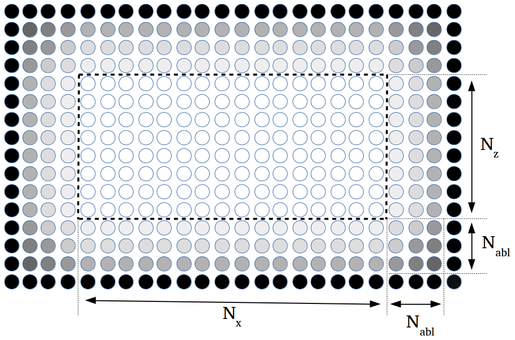
Figure 1 A vertical cross section of the computational mesh, along a y grid plane, where d is shown in a gray color scale. Finally, the black dots are nodes where pressure is forced to have a value of 0.

Figure 1 illustrates a 2D slice of such a grid. The area inside the dashed rectangle is the physical domain and the outside grid nodes belong to the absorbing layers and boundary. In the following we will consider that the extent of source terms is confined to the physical domain. Each grid node within the absorbing layers has a characteristic distance to the physical domain named d where $d_{i,j,l}=\sqrt{(d_{i,j,l}^x{)}^{\mathrm{2}}+(d_{i,j,l}^y{)}^{\mathrm{2}}+(d_{i,j,l}^z{)}^{\mathrm{2}}}$ and $d_{i,j,l}^{\mathit{\beta }}$ is the distance in grid nodes from $(i,j,l)$ to the closest node of the main grid in the $\mathit{\beta }\in \mathit{\{}x,y,z\mathit{\}}$ direction. In the figure, the gray scale represents the value of d at each point of the boundary layers. The definition of suitable absorption parameters for each ABL that depend explicitly on d, and become zero inside the main grid (i.e., when d=0), allows all ABL formulations in the following to use a global updating scheme. In other words, the same scheme is applied equally to all grid points in the computational domain, regardless of them being part of the physical domain or the absorbing layers.

There remains a last issue in order to solve the wave equation in the computational domain from parameters of the physical domain: the velocity $c(x,y,z)$ is only defined within the physical domain. However, we need to assign a velocity value to each node in the computational domain in order to solve the wave equation. We choose in the following a direct continuation strategy where all absorbing-layer nodes take their velocity value from the closest physical-domain grid-node velocity value. For a homogeneous model this results in the whole computational domain sharing the c value of the physical domain.

2.2 The damped wave equation (DWE)

The DWE is derived from the linear wave Eq. (3) by adding a dissipative term that depends on the first-order temporal derivative of the acoustic pressure and reads

$$\begin{array}{}\text{(5)}& {\displaystyle \frac{{\partial }^{\mathrm{2}}p}{\partial t^{\mathrm{2}}}}+\mathit{\sigma }{\displaystyle \frac{\partial p}{\partial t}}=c^{\mathrm{2}}\mathrm{\Delta }p,\end{array}$$

where $\mathit{\sigma }=\mathit{\sigma }(x,y,z)$ is the coefficient of the damping term.

We use the standard second-order and central FD approximations for both temporal derivatives in Eq. (5). Furthermore, we split the discrete acoustic pressure into Cartesian projections, i.e.,

$$\begin{array}{}\text{(6)}& p{|}_{i,j,l}^{n+\mathrm{1}}=p_x{|}_{i,j,l}^{n+\mathrm{1}}+p_y{|}_{i,j,l}^{n+\mathrm{1}}+p_z{|}_{i,j,l}^{n+\mathrm{1}},\end{array}$$

where these acoustic projections, $p_x{|}_{i,j,l}^{n+\mathrm{1}}$, $p_y{|}_{i,j,l}^{n+\mathrm{1}}$ and $p_z{|}_{i,j,l}^{n+\mathrm{1}}$, are updated according to

$$\begin{array}{ll}{\displaystyle }& {\displaystyle }{p}_x{|}_{i,j,l}^{n+\mathrm{1}}={\displaystyle \frac{{\mathit{\sigma }}_{i,j,l}{\mathit{\delta }}_{\mathrm{t}}-\mathrm{2}}{{\mathit{\sigma }}_{i,j,l}{\mathit{\delta }}_{\mathrm{t}}+\mathrm{2}}}{p}_x{|}_{i,j,l}^{n-\mathrm{1}}+{\displaystyle \frac{\mathrm{4}}{{\mathit{\sigma }}_{i,j,l}{\mathit{\delta }}_{\mathrm{t}}+\mathrm{2}}}{p}_x{|}_{i,j,l}^n\\ {\displaystyle }& {\displaystyle }+{\displaystyle \frac{\mathrm{2}(c_{i,j,l}{\mathit{\delta }}_{\mathrm{t}}{)}^{\mathrm{2}}}{{\mathit{\sigma }}_{i,j,l}{\mathit{\delta }}_{\mathrm{t}}+\mathrm{2}}}{\mathcal{F}}_x^{-\mathrm{1}}\left[{\left(\mathit{\iota }{k}_x\right)}^{\mathrm{2}}{\mathcal{F}}_x\left[p{|}_{:,j,l}^n\right]\right],\\ {\displaystyle }& {\displaystyle }{p}_y{|}_{i,j,l}^{n+\mathrm{1}}={\displaystyle \frac{{\mathit{\sigma }}_{i,j,l}{\mathit{\delta }}_{\mathrm{t}}-\mathrm{2}}{{\mathit{\sigma }}_{i,j,l}{\mathit{\delta }}_{\mathrm{t}}+\mathrm{2}}}{p}_y{|}_{i,j,l}^{n-\mathrm{1}}+{\displaystyle \frac{\mathrm{4}}{{\mathit{\sigma }}_{i,j,l}{\mathit{\delta }}_{\mathrm{t}}+\mathrm{2}}}{p}_y{|}_{i,j,l}^n\\ {\displaystyle }& {\displaystyle }+{\displaystyle \frac{\mathrm{2}(c_{i,j,l}{\mathit{\delta }}_{\mathrm{t}}{)}^{\mathrm{2}}}{{\mathit{\sigma }}_{i,j,l}{\mathit{\delta }}_{\mathrm{t}}+\mathrm{2}}}{\mathcal{F}}_y^{-\mathrm{1}}\left[{\left(\mathit{\iota }{k}_y\right)}^{\mathrm{2}}{\mathcal{F}}_y\left[p{|}_{i,:,l}^n\right]\right],\\ {\displaystyle }& {\displaystyle }{p}_z{|}_{i,j,l}^{n+\mathrm{1}}={\displaystyle \frac{{\mathit{\sigma }}_{i,j,l}{\mathit{\delta }}_{\mathrm{t}}-\mathrm{2}}{{\mathit{\sigma }}_{i,j,l}{\mathit{\delta }}_{\mathrm{t}}+\mathrm{2}}}{p}_z{|}_{i,j,l}^{n-\mathrm{1}}+{\displaystyle \frac{\mathrm{4}}{{\mathit{\sigma }}_{i,j,l}{\mathit{\delta }}_{\mathrm{t}}+\mathrm{2}}}{p}_z{|}_{i,j,l}^n\\ \text{(7)}& {\displaystyle }& {\displaystyle }+{\displaystyle \frac{\mathrm{2}(c_{i,j,l}{\mathit{\delta }}_{\mathrm{t}}{)}^{\mathrm{2}}}{{\mathit{\sigma }}_{i,j,l}{\mathit{\delta }}_{\mathrm{t}}+\mathrm{2}}}{\mathcal{F}}_z^{-\mathrm{1}}\left[{\left(\mathit{\iota }{k}_z\right)}^{\mathrm{2}}{\mathcal{F}}_z\left[p{|}_{i,j,:}^n\right]\right].\end{array}$$

We first update the acoustic projections by solving Eq. (7) and then compute the acoustic pressure at time tⁿ⁺¹ by means of Eq. (6), that results in an explicit time-marching method. Where ${\mathit{\sigma }}_{i,j,l}=\mathrm{0}$, the scheme reduces to a classical second-order-in- time explicit PSTD scheme for the second-order wave equation. In practical terms, DWE is applied to unbound wave propagation problems by assuming a zero σ inside the physical domain slowly increasing its value as we approach the boundary. The larger the value of σ the higher the absorption, although too steep a spatial change in σ can lead to artificial reflections. Here, we consider a linear variation of σ with respect to distance to the main grid of physical simulation, namely

$$\begin{array}{}\text{(8)}& {\mathit{\sigma }}_{i,j,l}={\mathit{\sigma }}_{\mathrm{0}}{\displaystyle \frac{d_{i,j,l}}{N_{\mathrm{ABL}}}}.\end{array}$$

We remark that we have found the dimensionless quantity σ₀δ_t better for the characterization of DWL absorption than σ₀; hence, when calibrating DWL we will use (N_ABL,σ₀δ_t) tuples to characterize different experiments for a fixed physical domain. Finally, it is worth mentioning that there exist other profiles that perform better. For example, Spa et al. (2014) suggest order 3 and 4 polynomial absorbing profiles. However, in this analysis, we chose a linear profile because we prefer to focus on both, the calibration methodology and the design of the numerical experiments, rather than on studying specific absorbing profiles of each method.

2.3 The sponge boundary layer (SBL)

Our second ABL under study is the SBL technique presented by Cerjan et al. (1985). The main formulation is based on the second-order wave equation for pressure p, but also requires its temporal derivative $\dot{p}$ as an auxiliary dependent variable. The reason for this requirement is that part of the damping is applied directly on $\dot{p}$. As a consequence, in PSTD we adopt a temporal staggered sampling of p and $\dot{p}$, so that both variables are computed with central differences of δ_t step. The time-marching algorithm consists of a two-step scheme, where $\dot{p}$ is computed at the temporal half step $n+\mathrm{1}/\mathrm{2}$, for a subsequent computation of p at the full step n+1. Similar to DWE, we also split both dependent variables into three Cartesian projections, and each projection is computed independently. The scheme starts with a first step

$$\begin{array}{ll}{\displaystyle }& {\displaystyle }{\dot{p}}_x{|}_{i,j,l}^{n+\frac{\mathrm{1}}{\mathrm{2}}}={\mathit{\mu }}_{i,j,l}\cdot {\dot{p}}_x{|}_{i,j,l}^{n-\frac{\mathrm{1}}{\mathrm{2}}}+{\mathit{\mu }}_{i,j,l}\cdot c_{i,j,l}^{\mathrm{2}}{\mathit{\delta }}_{\mathrm{t}}\\ {\displaystyle }& {\displaystyle }\cdot {\mathcal{F}}_x^{-\mathrm{1}}\left[{\left(\mathit{\iota }{k}_x\right)}^{\mathrm{2}}{\mathcal{F}}_x\left[p{|}_{:,j,l}^n\right]\right],\\ {\displaystyle }& {\displaystyle }{\dot{p}}_y{|}_{i,j,l}^{n+\frac{\mathrm{1}}{\mathrm{2}}}={\mathit{\mu }}_{i,j,l}\cdot {\dot{p}}_y{|}_{i,j,l}^{n-\frac{\mathrm{1}}{\mathrm{2}}}+{\mathit{\mu }}_{i,j,l}\cdot c_{i,j,l}^{\mathrm{2}}{\mathit{\delta }}_{\mathrm{t}}\\ {\displaystyle }& {\displaystyle }\cdot {\mathcal{F}}_y^{-\mathrm{1}}\left[{\left(\mathit{\iota }{k}_y\right)}^{\mathrm{2}}{\mathcal{F}}_y\left[p{|}_{i,:,l}^n\right]\right],\\ {\displaystyle }& {\displaystyle }{\dot{p}}_z{|}_{i,j,l}^{n+\frac{\mathrm{1}}{\mathrm{2}}}={\mathit{\mu }}_{i,j,l}\cdot {\dot{p}}_z{|}_{i,j,l}^{n-\frac{\mathrm{1}}{\mathrm{2}}}+{\mathit{\mu }}_{i,j,l}\cdot c_{i,j,l}^{\mathrm{2}}{\mathit{\delta }}_{\mathrm{t}}\\ \text{(9)}& {\displaystyle }& {\displaystyle }\cdot {\mathcal{F}}_z^{-\mathrm{1}}\left[{\left(\mathit{\iota }{k}_z\right)}^{\mathrm{2}}{\mathcal{F}}_z\left[p{|}_{i,j,:}^n\right]\right],\end{array}$$

where ${\mathit{\mu }}_{i,j,l}$ is a space-dependent absorption parameter, defined below, whereas the second step is

$$\begin{array}{ll}{\displaystyle }{p}_x{|}_{i,j,l}^{n+\mathrm{1}}& {\displaystyle }={\mathit{\mu }}_{i,j,l}\left[p_x{|}_{i,j,l}^n+{\mathit{\delta }}_{\mathrm{t}}\cdot {\dot{p}}_x{|}_{i,j,l}^{n+\frac{\mathrm{1}}{\mathrm{2}}}\right],\\ {\displaystyle }{p}_y{|}_{i,j,l}^{n+\mathrm{1}}& {\displaystyle }={\mathit{\mu }}_{i,j,l}\left[p_y{|}_{i,j,l}^n+{\mathit{\delta }}_{\mathrm{t}}\cdot {\dot{p}}_y{|}_{i,j,l}^{n+\frac{\mathrm{1}}{\mathrm{2}}}\right],\\ \text{(10)}& {\displaystyle }{p}_z{|}_{i,j,l}^{n+\mathrm{1}}& {\displaystyle }={\mathit{\mu }}_{i,j,l}\left[p_z{|}_{i,j,l}^n+{\mathit{\delta }}_{\mathrm{t}}\cdot {\dot{p}}_z{|}_{i,j,l}^{n+\frac{\mathrm{1}}{\mathrm{2}}}\right].\end{array}$$

Equations (9) and (10), followed by the step given by Eq. (6), result in an explicit time-marching scheme. In the present work we follow Cerjan et al. (1985) to define values of ${\mathit{\mu }}_{i,j,l}$ as follows:

$$\begin{array}{}\text{(11)}& {\mathit{\mu }}_{i,j,l}=e^{-{\left({\mathit{\mu }}_{\mathrm{0}}\cdot d_{i,j,l}\right)}^{\mathrm{2}}},\end{array}$$

where μ₀ is SBL's dimensionless absorption parameter. We will explore (N_ABL,μ₀) tuples for a fixed physical domain in upcoming sections. It is important to mention that this profile is neither polynomial nor dependent on N_ABL. As we mentioned in the previous subsection, we do not focus our attention on particular profiles but rather on a methodology to calibrate the main parameters. Definitely there should be a dependence between the parameter and N_ABL. However, as our methodology always analyzes tuples of N_ABL and the parameter, such dependence loses relevance, at least for our purposes.

2.4 The perfectly matched layer (PML)

The PML's formulation (Bérenger, 1994) requires first derivatives of the absorbed variables, in our case pressure p and velocity v. The first-order Euler formulation of the wave Eq. (2) involves all directional spatial derivatives required by the PML implementation, and thus it is natural to adopt this formulation for PML. The PSTD-PML method is a two-step time-staggered marching algorithm that first updates the particle velocity components,

$$\begin{array}{}\text{(12)}& \begin{array}{rl}& v_x{|}_{i+\frac{\mathrm{1}}{\mathrm{2}},j,l}^{n+\frac{\mathrm{1}}{\mathrm{2}}}=\\ & {\displaystyle \frac{\mathrm{1}}{\mathrm{1}+{\mathit{\alpha }}_{i,j,l}^x{\mathit{\delta }}_{\mathrm{t}}}}(v_x{|}_{i+\frac{\mathrm{1}}{\mathrm{2}},j,l}^{n-\frac{\mathrm{1}}{\mathrm{2}}}-{\displaystyle \frac{{\mathit{\delta }}_{\mathrm{t}}}{\mathit{\rho }}}\cdot {\mathcal{F}}_x^{-\mathrm{1}}\left[\mathit{\iota }{k}_x{\mathcal{F}}_x\left[p{|}_{:,j,l}^n\right]\right]),\\ & v_y{|}_{i,j+\frac{\mathrm{1}}{\mathrm{2}},l}^{n+\frac{\mathrm{1}}{\mathrm{2}}}=\\ & {\displaystyle \frac{\mathrm{1}}{\mathrm{1}+{\mathit{\alpha }}_{i,j,l}^y{\mathit{\delta }}_{\mathrm{t}}}}(v_y{|}_{i,j+\frac{\mathrm{1}}{\mathrm{2}},l}^{n-\frac{\mathrm{1}}{\mathrm{2}}}-{\displaystyle \frac{{\mathit{\delta }}_{\mathrm{t}}}{\mathit{\rho }}}\cdot {\mathcal{F}}_y^{-\mathrm{1}}\left[\mathit{\iota }{k}_y{\mathcal{F}}_y\left[p{|}_{i,:,l}^n\right]\right]),\\ & v_z{|}_{i,j,l+\frac{\mathrm{1}}{\mathrm{2}}}^{n+\frac{\mathrm{1}}{\mathrm{2}}}=\\ & {\displaystyle \frac{\mathrm{1}}{\mathrm{1}+{\mathit{\alpha }}_{i,j,l}^z{\mathit{\delta }}_{\mathrm{t}}}}(v_z{|}_{i,j,l+\frac{\mathrm{1}}{\mathrm{2}}}^{n-\frac{\mathrm{1}}{\mathrm{2}}}-{\displaystyle \frac{{\mathit{\delta }}_{\mathrm{t}}}{\mathit{\rho }}}\cdot {\mathcal{F}}_z^{-\mathrm{1}}\left[\mathit{\iota }{k}_z{\mathcal{F}}_z\left[p{|}_{i,j,:}^n\right]\right]),\end{array}\end{array}$$

to finally compute the values of each projection of the acoustic pressure,

$$\begin{array}{}\text{(13)}& \begin{array}{rl}& p_x{|}_{i,j,l}^{n+\mathrm{1}}=(\mathrm{1}-{\mathit{\alpha }}_{i,j,l}^x{\mathit{\delta }}_{\mathrm{t}})\cdot p_x{|}_{i,j,l}^n-\mathit{\rho }{c}_{i,j,l}^{\mathrm{2}}{\mathit{\delta }}_{\mathrm{t}}\\ & \cdot {\mathcal{F}}_x^{-\mathrm{1}}\left[\mathit{\iota }{k}_x{\mathcal{F}}_x\left[v_x{|}_{:,j,l}^{n+\frac{\mathrm{1}}{\mathrm{2}}}\right]\right],\\ & p_y{|}_{i,j,l}^{n+\mathrm{1}}=(\mathrm{1}-{\mathit{\alpha }}_{i,j,l}^y{\mathit{\delta }}_{\mathrm{t}})\cdot p_y{|}_{i,j,l}^n-\mathit{\rho }{c}_{i,j,l}^{\mathrm{2}}{\mathit{\delta }}_{\mathrm{t}}\\ & \cdot {\mathcal{F}}_y^{-\mathrm{1}}\left[\mathit{\iota }{k}_y{\mathcal{F}}_y\left[v_y{|}_{i,:,l}^{n+\frac{\mathrm{1}}{\mathrm{2}}}\right]\right],\\ & p_z{|}_{i,j,l}^{n+\mathrm{1}}=(\mathrm{1}-{\mathit{\alpha }}_{i,j,l}^z{\mathit{\delta }}_{\mathrm{t}})\cdot p_z{|}_{i,j,l}^n-\mathit{\rho }{c}_{i,j,l}^{\mathrm{2}}{\mathit{\delta }}_{\mathrm{t}}\\ & \cdot {\mathcal{F}}_z^{-\mathrm{1}}\left[\mathit{\iota }{k}_z{\mathcal{F}}_z\left[v_z{|}_{i,j,:}^{n+\frac{\mathrm{1}}{\mathrm{2}}}\right]\right].\end{array}\end{array}$$

Together with Eq. (6) we have a complete updating scheme. Above, the space-dependent parameter $\mathit{\alpha }=({\mathit{\alpha }}^x,{\mathit{\alpha }}^y,{\mathit{\alpha }}^z)$ is the vector quantity that controls PML absorption. Contrary to DWE or SBL, whose absorption depends, locally, only on the nodal distance to the main grid, in PML the outward direction from the physical domain is equally relevant. Similar to DWE (see Eq. 8), we define a linear increase in α components up to a maximum absorbing value α₀, i.e.,

$$\begin{array}{}\text{(14)}& {\mathit{\alpha }}_{i,j,l}={\mathit{\alpha }}_{\mathrm{0}}{\displaystyle \frac{d_{i,j,l}}{N_{\mathrm{ABL}}}}{\widehat{\mathit{d}}}_{i,j,l},\end{array}$$

where $\widehat{\mathit{d}}$ is the unit vector from $(i,j,l)$ to the closest point in the physical domain's grid, namely

$$\begin{array}{}\text{(15)}& {\widehat{\mathit{d}}}_{i,j,l}=\left({\displaystyle \frac{d^x}{d_{i,j,l}}},{\displaystyle \frac{d^y}{d_{i,j,l}}},{\displaystyle \frac{d^z}{d_{i,j,l}}}\right).\end{array}$$

Similar to DWL, we remark that we have found the dimensionless quantity α₀δ_t to be better at characterizing PML absorption than α₀; hence, when calibrating PML we will use (N_ABL,α₀δ_t) tuples to characterize different experiments for a fixed physical domain.

Finally, we mention that the velocity–pressure scheme Eqs. (12) and (13) is stated on a staggered spatial mesh, where shifting the spectral derivatives is critical to eliminate artifacts produced by the source generation, as previously reported in Ozdenvar and McMechan (1996).

2.5 Stability bound and dispersion error

Before our application exercises, we briefly comment on the stability of PSTD and its dispersion properties. At uniform grids and using second-order explicit time integration, a von Neumann analysis of PSTD in unbounded acoustic media yields the following bound for conditional stability:

$$\begin{array}{}\text{(16)}& S=max\mathit{\left\{}{c}_{i,j,l}\mathit{\right\}}{\displaystyle \frac{{\mathit{\delta }}_{\mathrm{t}}}{\mathit{\delta }}}\le {\displaystyle \frac{\mathrm{2}}{\mathit{\pi }\sqrt{\mathrm{3}}}}.\end{array}$$

In Eq. (16), S is the Courant–Friedrichs–Lewy (CFL) number. In the case of a homogeneous medium $c_{i,j,l}=c$, this theoretical analysis also leads to the following expression for dispersion errors:

$$\begin{array}{}\text{(17)}& {\displaystyle \frac{c_{\mathrm{num}}}{c}}={\displaystyle \frac{\mathit{\pi }{\mathit{\delta }}_{\mathrm{t}}}{T\sin \left(\frac{\mathit{\pi }{\mathit{\delta }}_{\mathrm{t}}}{T}\right)}}.\end{array}$$

Above, c_num is the numerical wave speed and T is the period of the given plane wave used in the von Neumann analysis. Thus, the spatial and temporal grid samplings must fulfill the inequality in Eq. (16) to guarantee stable simulations. However, the numerical accuracy of PSTD simulations is mainly driven by the dispersion errors quantified by Eq. (17), which only depend on the time step. As a consequence, in practical PSTD applications, the spatial step can be fixed to the largest value allowed by the Nyquist sampling limit, but the time step must be taken much smaller than the one allowed by the stability bound, in order to control dispersion anomalies. In other words, low-dispersive accurate PSTD simulations can be achieved using optimal S values, which are far below the limit established by Eq. (16). These von Neumann analytical results and suitable choices for space and time resolution are reported in the broad literature on PSTD methods (e.g., Gazdag, 1981; Fornberg, 1998, 1987; and also (Spa et al., 2020) for a recent review).

The coupling of the ABL techniques presented above to a PSTD method does not alter the stability and dispersion properties of PSTD in lossless unbound acoustic media. The physical attenuation experienced by acoustic waves at any frequency along the ABL regions only reinforces the boundedness of the numerical solution and thus favors the damping of short period oscillations induced by dispersion.

3 Calibration of ABL parameters

In the previous section we have written the formulations of all three ABL and remarked that two main parameters control absorption in each of them: the size of the absorbing layer N_ABL, which is a parameter shared by all ABLs, and a specific parameter that depends on each ABL, namely σ₀, μ₀ and α₀ for DWE, SBL, and PML, respectively. In the case of DWL and PML the absorption parameters have a dimension of inverse time; thus, in order to analyze absorption in a dimensionless framework we will use the tuples (N_ABL,σ₀δ_t), (N_ABL,μ₀), and (N_ABL,α₀δ_t) for DWE, SBL, and PML, respectively. Our study aims at characterizing the absorption profiles, namely absorption as a function of the tuples described above, of all three ABLs by means of experimentation. For homogeneous media, several authors have explored absorption parameter optimization through formal reflectivity and transmission analyses, for a particular ABL technique. For instance, Israeli and Orszag (1981), Kosloff and Kosloff (1986), and Spa et al. (2014) formally study damping profiles in the case of DWE, while analyses on PML parameterization for elastodynamics can be found in Chew and Liu (1996); Collino and Tsogka (2001). For seismic wave propagation,  Gao et al. (2017) compared the empirical performance of different absorbing techniques on acoustic heterogeneous test cases using finite difference methods.

3.1 Methodology

Our characterization effort involves (1) finding appropriate tests for which a reference exists, (2) finding suitable metrics that measure the absorption performance of the methods against the reference, (3) establishing absorption thresholds that classify the absorption, and (4) for each classification and ABL, finding the parameter tuple that requires the least absorption nodes or N_ABL. We will refer to such a tuple, for each ABL, as the optimal tuple. In this sense optimality refers to reaching the desired absorption with the minimum possible number of grid points.

The first step to create an absorption measure is quantifying the total energy in the physical domain (not including the ABL) at any given time sample. Thus, we define the following quantity which is proportional to the (discrete) ℒ² norm,

$$\begin{array}{}\text{(18)}& E{|}^n={\displaystyle }\sum _{i=\mathrm{1}}^{N_x}\sum _{j=\mathrm{1}}^{N_y}\sum _{l=\mathrm{1}}^{N_z}(p{|}_{i,j,l}^n{)}^{\mathrm{2}},\end{array}$$

and the corresponding dimensionless proxy,

$$\begin{array}{}\text{(19)}& \widehat{E}{|}^n={\displaystyle \frac{E{|}^n}{\underset{n\in [\mathrm{0},N_{\mathrm{t}}]}{max}E{|}^n}},\end{array}$$

where the energy E|ⁿ is normalized by the maximum energy value present in the problem. Another key ingredient to create an absorption measure consists of building a proper reference signal, namely ${\widehat{E}}_{\mathrm{REF}}$. Let us assume that this signal can be constructed whether numerical simulations or analytical expressions exist. In any case, the following quantity is defined:

$$\begin{array}{}\text{(20)}& \mathrm{\Delta }\widehat{E}=\sum _{n=n_{\mathrm{0}}}^{N_{\mathrm{t}}}\left|{\widehat{E}}_{\mathrm{REF}}{|}^n-\widehat{E}{|}^n\right|{\mathit{\delta }}_{\mathrm{t}}.\end{array}$$

Note that n₀ can be any value within the discrete time interval, and its value, as well as the computation of ${\widehat{E}}_{\mathrm{REF}}$, would be obtained depending on the specifications of the problem. For example, in problems where it is impossible to characterize the energy via analytical expressions, we will use numerical simulations to compute the reference solutions in the whole discrete time range, i.e., n₀=0. In these cases, when the scenarios and the source characterizations are complex, we will build reference solutions by considering simulations with a large number of ABLs compared with the original simulation carried out to obtain $\widehat{E}$. This way, we ensure lower contributions due to boundary reflections getting an idea about the sensitivity of the ABL implementation with respect to the number of absorbing nodes, N_ABL. In other words, $\mathrm{\Delta }\widehat{E}$ provides information on the differences between two signals: the computed signal, $\widehat{E}$; and the reference signal, ${\widehat{E}}_{\mathrm{REF}}$. It means that low values of $\mathrm{\Delta }\widehat{E}$ represent strong similarities on both signals, whereas high values of $\mathrm{\Delta }\widehat{E}$ exhibit differences between them.

On the other side, for problems where the domain has a constant propagation velocity, c, and the energy is injected by means of a source that is punctual and finite in time, we can obtain the time at which all energy should have left the computational domain under perfect absorption conditions. If we know when the source stops injecting energy and when the energy inside the physical domain must be zero (the time iteration n₀), we can assume that ${\widehat{E}}_{\mathrm{REF}}{|}^n=\mathrm{0}$ for n≥n₀ and, therefore, we define

$$\begin{array}{}\text{(21)}& \mathit{ϵ}=\log \left(\mathrm{\Delta }\widehat{E}\right)=\log \left(\sum _{n=n_{\mathrm{0}}}^{N_{\mathrm{t}}}\widehat{E}{|}^n{\mathit{\delta }}_{\mathrm{t}}\right).\end{array}$$

Instead of Eq. (20), which would be a measure of similarity between two signals, ϵ represents the remanent energy obtained due to the ABL approximation. In fact, it is worth pointing out that, under these conditions, the energy inside the physical domain at n≥n₀ should be null and, consequently, it means that Eq. (21) provides direct information about the absorbing features of the ABL implementation. Note that, in the next section, the calibration of the ABL approximations has been done by using the ϵ definition through Eq. (21). This way, we are able to measure the absorption performance of the three different methods under a same reference solution.

Moreover, it is important to highlight that the methodology for calibration of ABLs presented in this work is based on three main components: using representative models, establishing suitable metrics for absorption, and reducing the calibration to two parameters. We are not adding any assumptions regarding the underlaying PDEs used (linear acoustic waves, in our case). Similarly, there are no assumptions tied to the numerical method (pseudo-spectral time domain, in our case). Nevertheless, two modifications are foreseen for broadening the applicability of the method. On one hand, in the case of using other physical models, we would need to modify Eq. (21) with an alternate energy proxy. On the other hand, in the case of using other numerical methods, we may need to replace N_ABL with an alternative parameter that is a measure of the thickness of the ABL with respect to the minimum wavelength. The actual results of the calibration, of course, would be different for other PDEs and methods, but the calibration methodology is only expected to require the aforementioned, minor, modifications.

Finally, we mention that for all scenarios in the following, the main grid remains identical and we modify only the size of the ABL zone and its associated absorption parameter. We will always exploit the spatial discretization characteristics of PSTD, thus using the coarsest grid possible at 2 points per minimum wavelength (ppw). All sources used will be point sources in space and Ricker wavelets in time. All numerical experiments that follow use our bespoke PSTD-ABL implementations using the g++ C compiler version 4.5.3.1-1, under -lm and -O3 optimization flags, and linking the FFTW3 library version 3.3.4-2. All simulations have been performed by an Intel Core i7-6820HK processor running at 2.70GHz under the Linux operating system.

3.2 Calibration for a homogeneous cube

We first consider a cube $\mathrm{500}\times \mathrm{500}\times \mathrm{500}$ m³ with a constant wave velocity $c_{i,j,l}=\mathrm{2000}$ m s⁻¹, and place a point source at the central location. The source time function is a Ricker wavelet with the peak at 10 Hz, and hence a maximum frequency of ≈25 Hz, that excites a wavefield of minimum wavelength λ_min≈80 m. Note that we use a regularization of Dirac’s delta function for the spatial component of point sources, which is a Gaussian. In time we choose a Ricker wavelet which is the second derivative of a Gaussian. With this process, we attempt to avoid contributions beyond the Shannon-Nyquist sampling theorem.

We take a grid step of δ=40 m and a temporal step of δ_t=0.002 s, thus ensuring a stability number S=0.1 that is less than 30 % of the stability limit. For this example, the wavefields leave the main grid at n₀=208. This specific value of n₀ results from the maximum travel time from the source to the corners of the domain (108 time steps) and the time needed to finish injecting 95 % of the energy from the source wavelet (100 time steps). After n₀ the remaining energy in the domain comes from reflections at the ABL. As mentioned, we use Eq. (21) to measure the absorption performance of the ABL implementations.

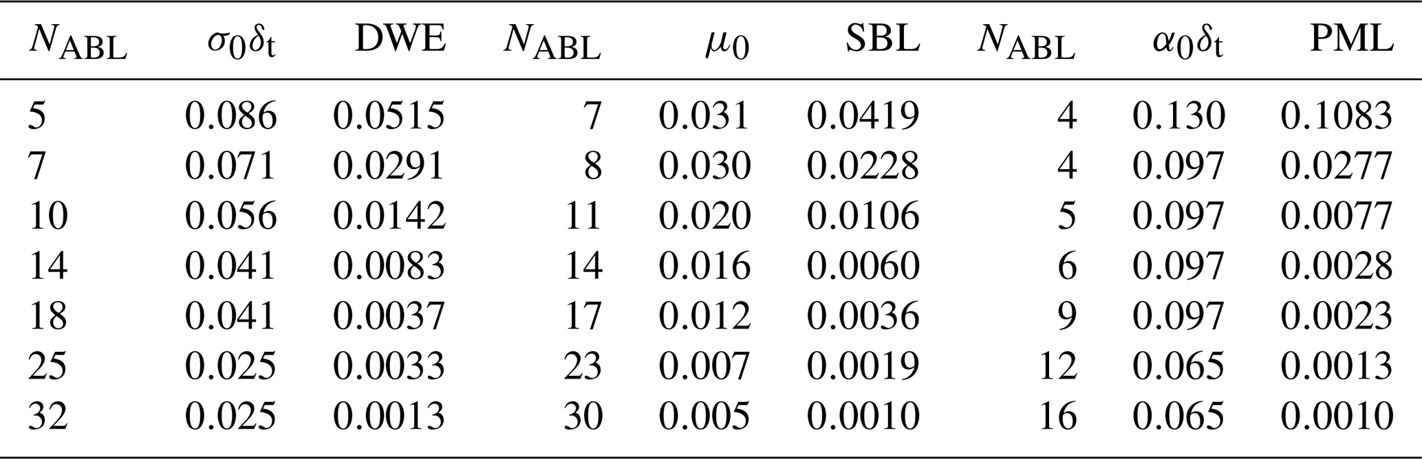
Next, we perform a numerical exploration of the N_ABL-absorption parameter pairs, using the samples in Table 1. For each ABL, we vary both N_ABL and their respective absorption parameter, thus resulting in 620 scenarios per ABL.

Table 1 Sampling of the absorption parameters and absorbing layer size used for parameter exploration for each ABL.

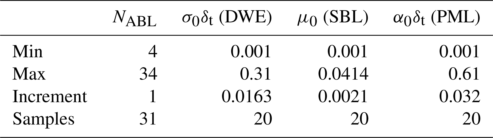
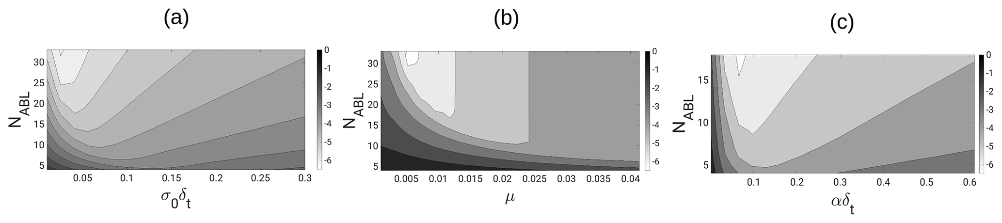
Figure 2 The gray scale depicts ϵ as a function of N_ABL and the absorption parameters for (a) DWE, (b) SBL, and (c) PML. Lighter gray indicates better absorption. Notice the smaller number of absorbing layers (vertical axis) used by PML.

Figure 2 depicts ϵ values for the parameter ranges considered in Table 1 that include results for DWE (Fig. 2a), SBL (Fig. 2b), and PML (Fig. 2c) techniques. In the case of PML we restrict the vertical axis to N_ABL≤16 as this results in already sufficient absorption of wavefields. For all cases there is an increase in absorption with N_ABL and we have a window of optimal absorption parameters which depends mildly on N_ABL. All ABL methods reach an absorption performance of $\mathit{ϵ}<-\mathrm{6}$ in the explored N_ABL range. PML is the most efficient technique because it only requires N_ABL=16 to achieve this ϵ threshold. Alternatively, DWE reaches the same absorption using N_ABL=32, while SBL employs N_ABL=30. Both PML and DWE absorption improve consistently with N_ABL. Conversely, SBL seems less sensitive to increasing N_ABL and absorption seems to saturate after a given N_ABL value.

Table 2 Optimal pairs of N_ABL and associated ABL parameters found for each ϵ threshold.

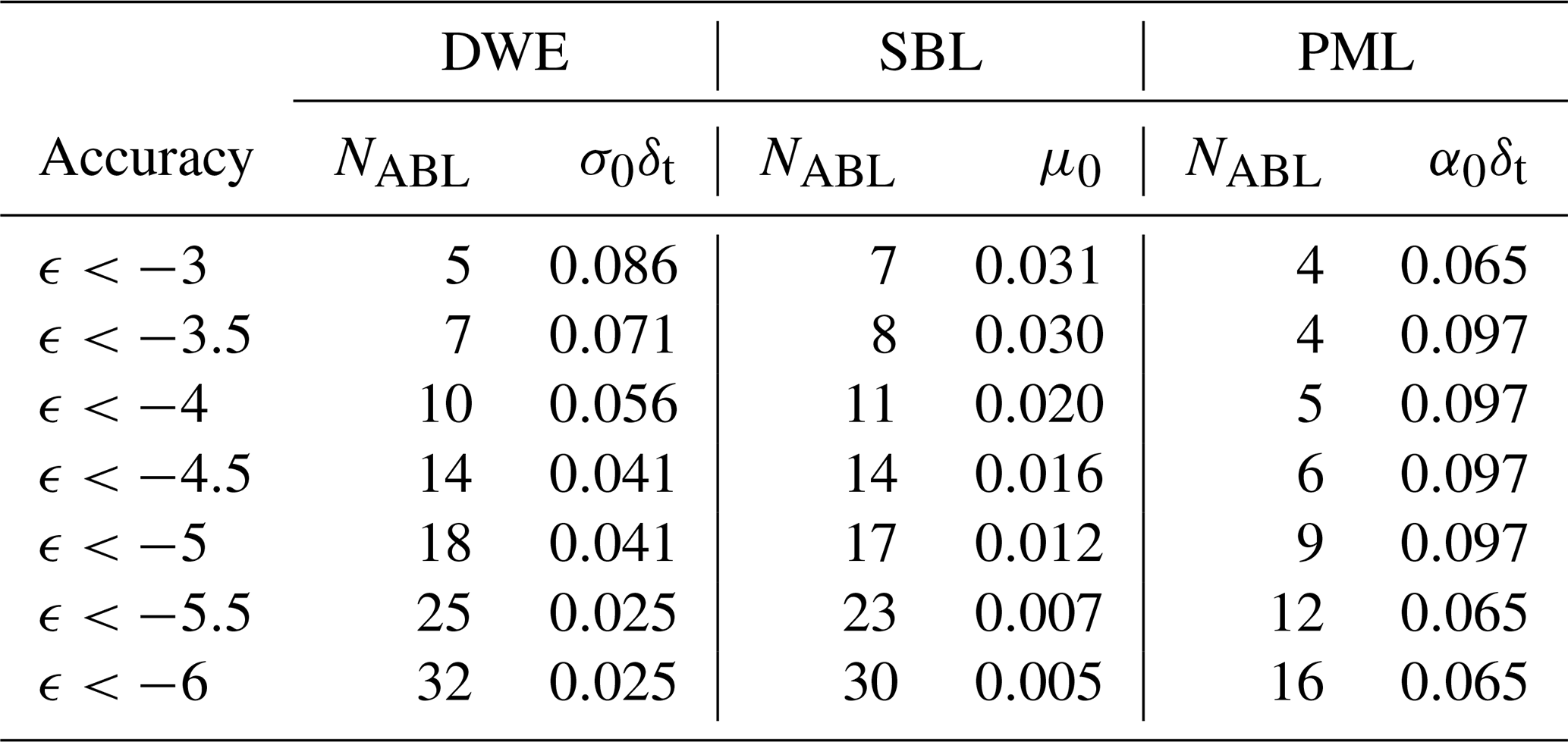
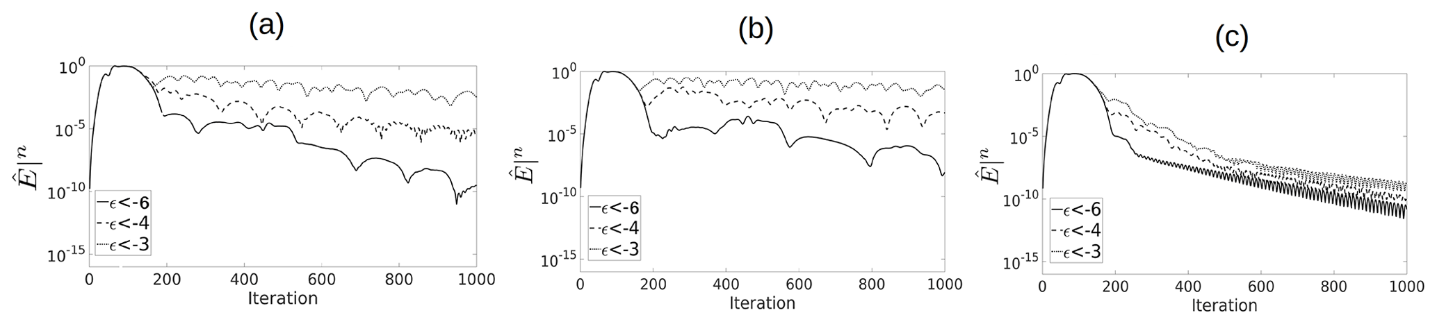
Figure 3 The time evolution of the energy proxy $\widehat{E}{|}^n$ in logarithmic scale for the (a) DWE, (b) SBL, and (c) PML techniques. The ABL parameters are set as per Table 2.

Table 2 shows, for several ϵ thresholds, which is the minimum N_ABL and coupled absorption parameter value. In the threshold range $-\mathrm{6}<\mathit{ϵ}<-\mathrm{3.5}$, DWE and PML deliver comparable accuracy, but the former needs at least twice the N_ABL value than the latter. Relative to DWE, SBL achieves the same absorption for nearly similar N_ABL.

Finally, Fig. 3 compares the time evolution of our energy proxy $\widehat{E}{|}^n$ for each ABL technique, for three ϵ threshold values given in Table 2. For each ABL technique, significant differences in the $\widehat{E}$ magnitude among these three curves are observed early, soon after n₀ iterations. In the DWE and SBL cases, large differences in the absorption efficiency persist during all N_t=1000 iterations, but slighter differences are observed in PML curves. In the next section, these three reference parameter sets will be exercised and compared in ABL applications to heterogeneous test cases.

3.3 Accuracy analysis for geophysical imaging

In addition to sheer energy absorption, it is important to analyze the impact of our different ABLs in practical imaging applications. As a simple yet representative test, we analyze a reverse time migration (RTM) case in a homogeneous model with a single source and receiver. In reverse-time migration (e.g., see Claerbout et al., 1985) an image, or reflectivity map, of the subsurface is obtained by means of two seismic simulations. A forward simulation propagates the source wavelet signal through the domain of interest, whereas a backward simulation propagates the data recorded in the field for that same source, reverted in time. By correlating the wavefields of forward and (time-reversed) backward simulations we generate the image of the subsurface, which indicates regions of impedance in the subsurface that may have generated the observed data. RTM has the advantage over other imaging modalities of supporting completely heterogeneous 3D velocity models, as well as incorporating all finite-frequency phenomena associated with acoustic waves, such as multiple reflections or scattering. On the other hand, it is costly in terms of computation (it relies on simulations) and inherits all inaccuracies of the wavefield simulation algorithms (e.g., imperfect boundaries) which may result in artifacts in the image. A calibration exercise frequent to imaging, and specifically to RTM, is known as impulse response imaging (see, for instance, Claerbout et al., 1985; Ng, 2007). In an impulse response a single-source image is generated by placing a single hypothetical receiver at the same location as the source. The receiver may include several well-known pulses, which when imaged into the domain of interest result in patterns that can be analyzed to assess how accurately images can be obtained at different depths. For a homogeneous-model impulse response, there is no preferred origin for the reflections, which are imaged as concentric half spheres of finite width centered at the source location, which coincides with the receiver location. Furthermore, the amplitude of the resulting image is independent of energy spread, and thus any disagreement between the expected and modeled image is due to modeling errors. In our case, we choose to investigate the vertical image column of the impulse response image that contains the source (and receiver). For such simple configuration it is easy to obtain an exact solution to the problem, and hence we can use a time–frequency analysis Kristekova et al. (2006) to check the quality of our image. Time–frequency analysis typically refers to temporal signals. As in our case the image exists in the spatial domain, we can refer to an analogous space–wavenumber analysis.

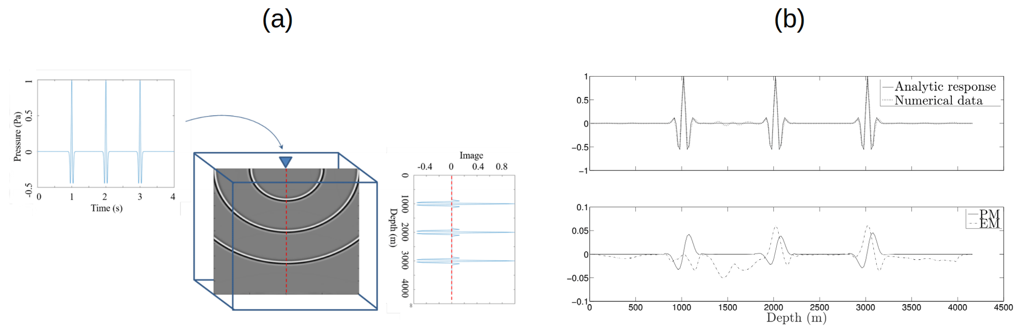
Figure 4 Panel (a) shows a reflectivity image (in grayscale) from an impulse response in homogeneous media, with the receiver data in horizontal and a close-up of the exact image column in vertical. Panel (b) shows an example of image column results compared with the exact reference (top) and the envelope and phase errors between them (bottom). The discrete sum of the error curves results in EM and PM, respectively.

We use the same model, grid steps δ and δ_t, and wavelet as in Sect. 3.2 with the following exceptions: the domain size is enlarged to $\mathrm{4}\times \mathrm{4}\times \mathrm{4}$ km³ and the source is placed at $(\mathrm{2},\mathrm{2},\mathrm{0})$ km. A receiver is located at the same point as the source. The data signal in this impulse response study contains three pulses, equal in shape to the source wavelet, but with peaks at 1, 2, and 3 s, respectively (see Fig. 4a). Given the homogeneous velocity 2000 m s⁻¹, the data are mapped in the image as three concentric half spheres centered at the source location, which coincides with the receiver location, and with radii 1, 2, and 3 km, respectively (see Fig. 4). These particular radii are the distances compatible with acoustic reflectors generating the data (i.e., three wiggles, at 1, 2, and 3 s). In order to assess the accuracy of the ABLs, we use the same ABL parameterizations obtained in Sect. 3.2 (see Table 2) and we measure both envelope (EM) and phase (PM) misfits with respect to the reference solution.

Table 3 Envelope misfits (EM) and phase misfits (PM) obtained when using the three ABL techniques under different ϵ accuracy thresholds. Both EM and PM are dimensionless quantities.

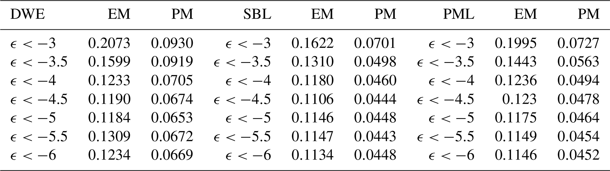
Table 3 presents the results in terms of EM and PM with respect to the absorption configurations found in Table 2. As expected, and further validating the findings of Sect. 3.2, for high ϵ thresholds the misfits EM and PM are small. Both errors decrease monotonically for PML, whereas misfits delivered by SBL and DWE show some oscillations in the range $-\mathrm{6}<\mathit{ϵ}<-\mathrm{5}$. In all cases, we find SBL performing slightly better than both DWE and PML, and in the case of the highest absorption, $\mathit{ϵ}<-\mathrm{6}$, its performance is comparable to that of PML for both PM and EM metrics. We can thus conclude that the parameterization pairs obtained in the previous sections result in better image accuracy as the absorption of the ABLs increases, i.e., as the ϵ threshold decreases.

As an additional comparison, we compute the same impulse response exercise using an algorithm popular in geophysical imaging: finite differences with eighth order in space and second order in time, using δ=20 m and δ_t=0.003454 s. In this case we obtain EM∼0.14 and PM∼0.07 when using second-order Higdon paraxial ABCs. Both numbers can be matched, and improved, by using the algorithms presented here. Notice that the spatial grid of this alternative scheme is considerably larger that the one used with the PSTD method presented in this study, due to the higher points per wavelength needed in finite-difference schemes.

4 Validation of ABL parameters in heterogeneous media

The earth's subsurface is largely heterogeneous across many scales. In such environments wavefields become more complex, involving scattering, reflections, and refractions, among other phenomena. As a consequence, a generalized calibration of ABLs is not possible, as all models are fundamentally different from each other. Our goal when studying ABLs in heterogeneous media is assessing whether their fundamental behavior remains, i.e., absorption increases steadily with N_ABL, and if our calibration results, which were obtained for homogeneous models, are also useful for heterogeneous models. We remark that we will use a direct continuation strategy to populate velocity values at the absorbing layers, as defined in the first subsection of Sect. 2.

4.1 Three-layered medium

First, we consider a 3D cuboid physical domain involving three flat layers of wave speeds 2000, 4000, and 6000 m s⁻¹, respectively. The central layer is 1320 m thick, with the top and bottom layers both being half spaces. The source parameters and the size of the domain is the same as in Sect. 3.2. However, in this test case, the Ricker point source is located 1300 m above the first material interface, and therefore inside the top layer, but still central in the other two directions. We run simulations for N_t=5000 iterations for a total simulation time of 10 s.

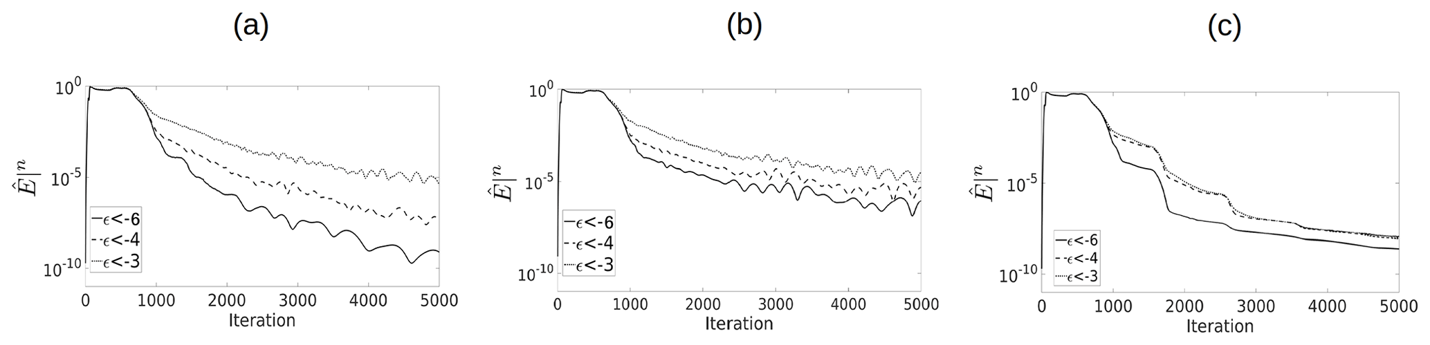
Figure 5 The time evolution of the energy proxy $\widehat{E}{|}^n$ in logarithmic scale for the three-layered test using (a) DWE, (b) SBL and (c) PML. ABL parameters are set as per Table 2.

In Fig. 5, we show the evolution of our energy proxy $\widehat{E}{|}^n$ during the simulation time. We observe $\widehat{E}{|}^n$ diminishing for all cases after the first approximately 1000 iterations. The rate at which $\widehat{E}{|}^n$ is reduced afterwards depends on the ABL and the threshold used. We remark that the ABLs are parameterized following Table 2. Consistent with previous observations in Fig. 3 for homogeneous media, lower ϵ thresholds result in better absorption. In addition, if we focus on long-term absorption (i.e., at iteration 5000 or $\widehat{E}{|}^{\mathrm{5000}}$), DWE at $\mathit{ϵ}<-\mathrm{6}$ reaches the smallest energy proxy values among all methods and configurations, whereas PML delivers small energy proxy values regardless of the parameter configuration chosen. DWE appears to be the most sensitive ABL to parameter changes, having the largest difference between best and worse absorption among all methods tested.

4.2 The SEG/EAGE salt model

As a final and more realistic scenario, we use the 3D SEG/EAGE salt model (e.g., see Yoon et al., 2003) and test our ABL for a modeling exercise. This model has been extensively used for benchmarking exercises in geophysics because it includes features typically observed in the subsurface. The model dimensions are $(\mathrm{7.5},\mathrm{7.5},\mathrm{3.6})$ km and we locate a point source at $(x_{\mathrm{s}},y_{\mathrm{s}},z_{\mathrm{s}})=(\mathrm{3.75},\mathrm{3.75},\mathrm{0})$ km. In this model, the wave speed varies from 1500 m s⁻¹ at the top water layer to 4200 m s⁻¹ inside the salt body (see Fig. 6). We add an ABL to each boundary of the physical model resulting in an unbounded domain. We remark that we are not adding a free surface condition to be compatible with the calibration exercise of the previous sections which also were unbounded. As in previous experiments, we use a Ricker source wavelet with a maximum frequency of 25 Hz and adapt the grid spacing to δ=30 m to accommodate the model's minimum velocity. Similarly, the time discretization is δ_t=0.002 s, which results in a maximum stability number S=0.28. In this test case, PSTD simulations last for 4 s, i.e., they involve N_t=2000 time iterations.

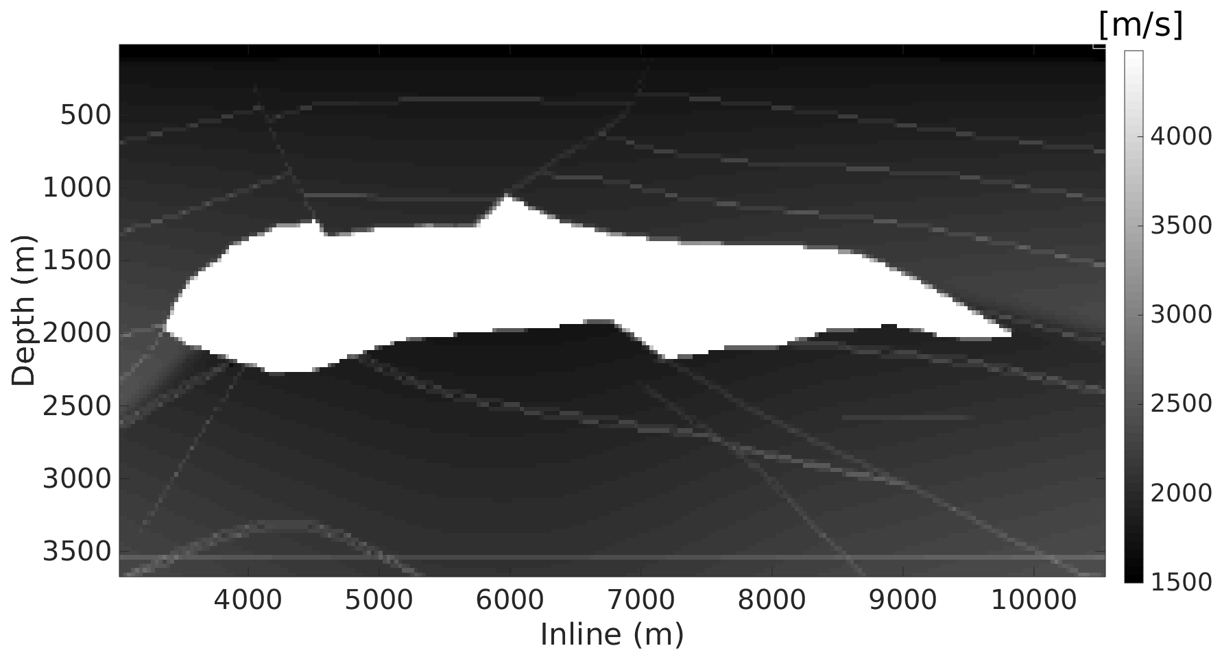
Figure 6 A vertical cross section, along the zx plane located at y=6800 m, of the 3D SEG/EAGE salt velocity model. The white (high-velocity) part is a salt body.

In order to quantify the absorption for such a complex model, we need to run several configurations of ABLs and compare them with a reference. To construct such a reference solution, we use the PSTD simulation that employs PML using the parameters associated with maximum absorption in Table 2 and N_ABL=120. Absorption for each ABL is next quantified using this reference. As illustration, Fig. 7 compares the wavefield at time step 430 (t=0.86 s) obtained when using the best DWE configuration reported in Table 2 with the reference solution. Specifically, Fig. 7a uses DWE with σ₀δ_t=0.0025 and N_ABL=32, whereas Fig. 7b uses the reference PML configuration. Figure 7c shows the difference between these two snapshots at this time step. Most differences appear from a reflected wavefront by the top ABL in simulations using DWE. As the PSTD algorithm and simulation parameters are identical, i.e., time and grid stepping, these differences arise from the less effective absorption achieved by DWE.

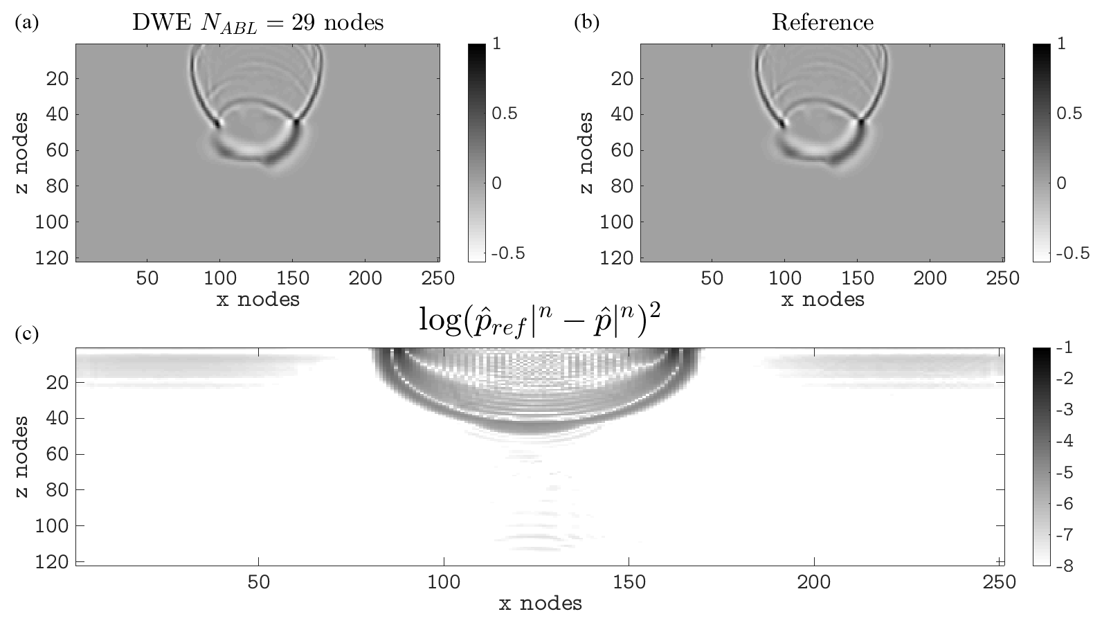
Figure 7 Snapshots of pressure at t=0.86 s using (a) DWE with σ₀δ_t=0.025 and N_ABL=32 and (b) PML with α₀δ_t=0.065 and N_ABL=120. Panel (c) shows their difference $({\widehat{p}}_{\mathrm{ref}}{|}^n-\widehat{p}{|}^n{)}^{\mathrm{2}}$ in a logarithmic scale.

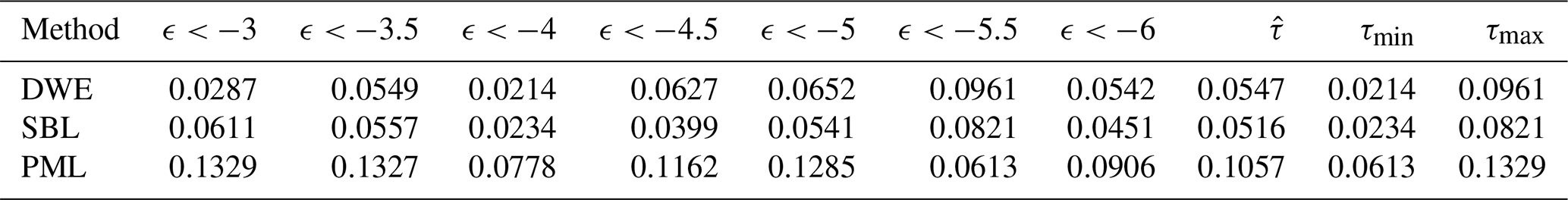
We run simulations using all three ABLs using all absorption parameter pairs reported in Table 2 and compute the corresponding errors using the metric defined in Eq. (20) for n₀=0 and the reference solution based on PML. The results are reported in Table 4 for all cases. For each ABL, errors steadily diminish with lower ϵ thresholds, i.e., as we sequentially employ the optimal parameter pairs given in Table 2. This is a remarkable result, as it confirms the results from Sect. 3.2, i.e., we can use the calibration parameters obtained from a homogeneous case and observe improvements in absorption in a complex heterogeneous case. Results in Table 4 are also consistent with the absorption improvements achieved by using the three parameter choices employed in the previous three-layered medium test. Finally, note that under the same ϵ threshold, most PML errors in Table 4 are smaller than those reported by SBL, while DWE delivers the bigger errors. However, the slightly lower efficiency of DWE compared with SBL might be related to this particular SEG/EAGE model, and results can be reversed in a different seismic scenario, as already observed in the three-layered test (see Fig. 5).

Table 4 Errors $\mathrm{\Delta }\widehat{E}$ computed on the SEG/EAGE 3D salt model using the absorption parameter pairs reported in Table 2.

5 Comments on the computational times of ABL techniques

In this section, we discuss the computational times obtained for our different ABLs coupled with PSTD acoustic wave simulations. Of course, observations in terms of computational time are less objective measures, because times are affected by the algorithm design, compilation optimization, coding skills, and libraries employed; hence, we do not suggest that our findings are universal. Nevertheless, we start our analysis with two theoretical aspects or considerations. Finally, we remark that for all methods, we solve the complete absorbing equation for each grid node, only using non-zero values for the absorption parameters inside the absorbing layers.

First, we consider the memory footprint of PSTD using the three ABLs. As formulated in Sect. 2, our three ABLs require storage of seven 3D arrays. Each array covers the computational domain of size $(N_x+\mathrm{2}{N}_{\mathrm{ABL}})(N_y+\mathrm{2}{N}_{\mathrm{ABL}})(N_z+\mathrm{2}{N}_{\mathrm{ABL}})$. In particular, DWE uses $p_x{|}^{n+\mathrm{1}}$, $p_y{|}^{n+\mathrm{1}}$, $p_z{|}^{n+\mathrm{1}}$, p_x|ⁿ, p_y|ⁿ, p_z|ⁿ, p|ⁿ, SBL uses $p_x{|}^{n+\mathrm{1}}$, $p_y{|}^{n+\mathrm{1}}$, $p_z{|}^{n+\mathrm{1}}$, ${\dot{p}}_x{|}^{n+\mathrm{1}}$, ${\dot{p}}_y{|}^{n+\mathrm{1}}$, ${\dot{p}}_z{|}^{n+\mathrm{1}}$,p|ⁿ, and PML uses $p_x{|}^{n+\mathrm{1}}$, $p_y{|}^{n+\mathrm{1}}$, $p_z{|}^{n+\mathrm{1}}$, $v_x{|}^{n+\mathrm{1}/\mathrm{2}}$, $v_y{|}^{n+\mathrm{1}/\mathrm{2}}$, $v_z{|}^{n+\mathrm{1}/\mathrm{2}}$, p|ⁿ.

Second, we consider the amount of operations required per time update. Both DWE and SBL compute a single 1D spectral derivative of p|ⁿ along each coordinate, while PML computes an additional differentiation for each velocity component. Therefore, DWE and SBL benefit from the second-order linear wave equation formulation and require half the number of Fourier transforms than the PML-based algorithm, which relies on the first-order Euler formulation. Although the previous theoretical discussion considers the same number of absorbing layers for all methods, we must recall that in Sects. 3.2 and 4 we have consistently observed that PML requires about half the absorbing layers N_ABL than either DWE or SBL for the same absorption. Nevertheless, given the usual size of geophysical domains, which are much larger than the number of layers considered in ABLs (i.e., $N_x,N_y,N_z\mathit{>>}{N}_{\mathrm{ABL}}$), this aspect does not result in a substantial advantage for PML in terms of memory or computational time.

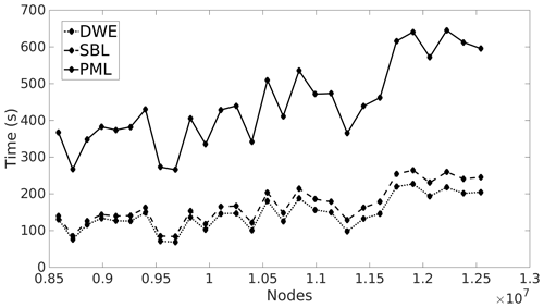
Figure 8 Computational time of all ABLs at different grids, characterized by their total number of nodes.

Table 5 Relative computing time τ with respect to the reference solution for experiment 1 in Sect. 4.2. All ABL parameters follow ϵ thresholds in Table 2. Average, minimum, and maximum times are included in the last three columns, respectively.

Following the theoretical discussion, we have measured computational times for our PSTD code using the three ABLs for different grid sizes. In Fig. 8, we present the computational times of 28 different grids using the setup of experiment 1 in Sect. 4. The total number of nodes in the grid is defined as $(N_x+\mathrm{2}{N}_{\mathrm{ABL}})(N_y+\mathrm{2}{N}_{\mathrm{ABL}})(N_z+\mathrm{2}{N}_{\mathrm{ABL}})$ and N_ABL ranges from 4 to 31. Three conclusions can be drawn from the figure: (1) computational cost increases, on average, with grid size, as expected; (2) PML takes approximately twice as long as either SBL or DWE for the same grid size; and (3) there is an important variability in computational cost from the average trend, of about 15 %–20 % with respect to the average value. The variability is very similar for all three ABLs at a single grid and, hence, stems from the node count and not other specific aspects of the different ABLs. This last result can be surprising when compared with other computational methods, such as finite differences or finite elements, but stems from the complex heuristics of modern FFT and DFT implementations, as will be further discussed later in this section. We remark that we use the FFTW3 library version 3.3.4-2 in our study.

To further expand our cost analysis we present results for our experiments in Sect. 4 comparing computational times for several ABL configurations relative to those obtained at the reference domain. Such a relative time metric is referred to as τ. In Table 5 we show relative times for all parametric cases, as well as their average $\widehat{\mathit{\tau }}$ and both minimum and maximum, i.e., τ_min and τ_max, respectively, among all parameterizations used. In the table, we observe that average times $\widehat{\mathit{\tau }}$ for PML are about twice those of $\widehat{\mathit{\tau }}$ for the other two ABL approaches, as expected from our previous analysis and consistent with Fig. 8. For increasing absorption ranges in Table 5, we require N_ABL to be larger for all ABLs. Although in other seismic modeling methods this would result in a consistent increase in computational time, this is not the case for PSTD. Computational times are rather scattered and do not increase monotonically with respect to ϵ thresholds. The explanation for this result, consistent with what is observed in Fig. 8, is the following: novel FFT libraries rely on different factorizations and algorithms in order to optimize time to solution for each node count. This results in FFTs that are very fast but also highly susceptible to significant variations as a function of the node count. We rely on FFTW3 in our case, but similar behavior is observed in other contemporary FFT libraries (e.g., see Khokhriakov et al., 2018 for an example using Intel MKL) and should be considered normal for PSTD or other Fourier-based methods. As a final recommendation, given the small value of N_ABL with respect to the main grid dimensions in geophysical applications, it might be beneficial to test different N_ABL values to reduce computational cost while keeping similar absorption.

6 Conclusions

In this work, we have reviewed and compared the three main ABL methodologies available in the context of PSTD simulations for acoustic wave propagation. Specifically, the damped wave equation, the sponge boundary layer proposed in Cerjan et al. (1985), and a classical split perfectly matched layer formulation, have been developed and their algorithms outlined. The three ABLs are relevant because they allow us to keep a pure Fourier pseudo-spectral scheme without hybrid approximations at the boundaries. Absorption of DWE, SBL, and PML is controlled by the number of layers N_ABL and a single parameter specific to each formulation, i.e., σ₀δ_t, μ₀ and α₀δ_t for DWE, SBL, and PML, respectively. We have performed a calibration study on a simple homogeneous medium, extracting optimal configurations (i.e., those with minimum boundary size N_ABL) for a series of energy absorption thresholds. To that end, such configurations have been tested in a series of exercises of different heterogeneity distributions and complexity. We have established that configurations that resulted in high absorption in our calibration, which involved a cube with homogeneous properties and just measured reflected energy, allow us to: (1) obtain better quality in a seismic imaging exercise, both in terms of phase and amplitude; (2) achieve better absorption also in a three-layered model, despite the change in space/time sampling required by the heterogeneity and the more complex wavefields involved such as reflections and refractions; and (3) accomplish better absorption in a complex 3D heterogeneous case. Hence, we can conclude that the configurations obtained in our simple calibration study lead to increased quality of results for all cases tested. Such configurations are meant to be guidelines for modeling or imaging practitioners and can be specialized to fit their accuracy needs.

Comparing the three ABLs with each other is a complex issue. On one hand, DWE and SBL have very similar formulations and behave similarly in terms of N_ABL for a given absorption threshold and computational cost. On the other hand, PML requires fewer boundary layers for the same absorption level at the price of a higher overall computational cost, approximately double that of DWE and SBL. Among these ABL methods, SBL presents less sensitivity to the increment of N_ABL.

To assess absorption performance, we have introduced a dimensionless measure proportional to the total acoustic energy in the seismic volume and use its magnitude in the calibration of ABL parameters. This energy proxy is consistent with the reflected energy that we qualitatively observe in all test scenarios, and therefore we recommend it for similar studies of absorption methods. The methodology to calibrate ABLs in this work could be applied to other wave equations such as the elastic wave equation or anisotropic wave equation. We do not expect the same calibration values to hold across all the equations, but the methodology should reveal the optimal values for each case. This will be the subject of future work.

We remark that computational times increase with grid size, but not in a steady or monotonic way, as a result of using modern FFT libraries. Therefore, varying the absorption of ABLs by means of larger N_ABL values does not necessarily result in increased computational time. Ultimately, computational times are not strictly predictable, other than PML being significantly more expensive than either DWE or SBL in terms of computational time.