the Creative Commons Attribution 4.0 License.
the Creative Commons Attribution 4.0 License.
 | 29 Nov 2023
A high-resolution physical–biogeochemical model for marine resource applications in the northwest Atlantic (MOM6-COBALT-NWA12 v1.0)
Andrew C. Ross
Charles A. Stock
Alistair Adcroft
Enrique Curchitser
Robert Hallberg
Matthew J. Harrison
Katherine Hedstrom
Niki Zadeh
Michael Alexander
Wenhao Chen
Elizabeth J. Drenkard
Hubert du Pontavice
Raphael Dussin
Fabian Gomez
Jasmin G. John
Dujuan Kang
Diane Lavoie
Laure Resplandy
Alizée Roobaert
Vincent Saba
Sang-Ik Shin
Samantha Siedlecki
James Simkins
We present the development and evaluation of MOM6-COBALT-NWA12 version 1.0, a ∘ model of ocean dynamics and biogeochemistry in the northwest Atlantic Ocean. This model is built using the new regional capabilities in the MOM6 ocean model and is coupled with the Carbon, Ocean Biogeochemistry and Lower Trophics (COBALT) biogeochemical model and Sea Ice Simulator version-2 (SIS2) sea ice model. Our goal was to develop a model to provide information to support living-marine-resource applications across management time horizons from seasons to decades. To do this, we struck a balance between a broad, coastwide domain to simulate basin-scale variability and capture cross-boundary issues expected under climate change; a high enough spatial resolution to accurately simulate features like the Gulf Stream separation and advection of water masses through finer-scale coastal features; and the computational economy required to run the long simulations of multiple ensemble members that are needed to quantify prediction uncertainties and produce actionable information. We assess whether MOM6-COBALT-NWA12 is capable of supporting the intended applications by evaluating the model with three categories of metrics: basin-wide indicators of the model's performance, indicators of coastal ecosystem variability and the regional ocean features that drive it, and model run times and computational efficiency. Overall, both the basin-wide and the regional ecosystem-relevant indicators are simulated well by the model. Where notable model biases and errors are present in both types of indicator, they are mainly consistent with the challenges of accurately simulating the Gulf Stream separation, path, and variability: for example, the coastal ocean and shelf north of Cape Hatteras are too warm and salty and have minor biogeochemical biases. During model development, we identified a few model parameters that exerted a notable influence on the model solution, including the horizontal viscosity, mixed-layer restratification, and tidal self-attraction and loading, which we discuss briefly. The computational performance of the model is adequate to support running numerous long simulations, even with the inclusion of coupled biogeochemistry with 40 additional tracers. Overall, these results show that this first version of a regional MOM6 model for the northwest Atlantic Ocean is capable of efficiently and accurately simulating historical basin-wide and regional mean conditions and variability, laying the groundwork for future studies to analyze this variability in detail, develop and improve parameterizations and model components to better capture local ocean features, and develop predictions and projections of future conditions to support living-marine-resource applications across timescales.
- Article
(10630 KB) - Full-text XML
- BibTeX
- EndNote


Over the last few decades, the northwest Atlantic Ocean has experienced prominent variability and sharp trends driven by climate change and other anthropogenic factors, shifting currents, and basin-scale modes of climate variability. Sea surface temperatures in the Gulf of Maine and Scotian Shelf and slope regions, located within the Northeast US Large Marine Ecosystem (LME), warmed faster than the vast majority of the global ocean in the last 2 decades (Pershing et al., 2015; Seidov et al., 2021). In addition to being driven by a warming atmosphere caused by increasing greenhouse gas concentrations, some of this warming occurred abruptly following shifts in the Gulf Stream path (Friedland et al., 2020a, b). The destabilization point of the Gulf Stream has recently moved westward, closer to where it separates from the continental shelf (Andres, 2016), and more frequent intrusions of warm and saline water onto the shelf (Gawarkiewicz et al., 2022) and eddy shedding (Gangopadhyay et al., 2019, 2020) have been observed. Northward shifts of the Gulf Stream have cut off the cool, southward Labrador Current and amplified warming in the region (Brickman et al., 2018; Gonçalves Neto et al., 2021; Seidov et al., 2021), although some studies have found contrasting long-term trends in the latitudinal position of the Gulf Stream (Wang et al., 2022). Sea surface temperatures have also been observed to be warming faster than the global average in the Gulf of Mexico (Wang et al., 2023) and Caribbean Sea (Glenn et al., 2015). Rising temperatures and changes in ocean dynamics have contributed to a rapid increase in sea level and coastal flooding risk along most of the US East Coast (Ezer and Atkinson, 2014).
Basin-scale modes of climate variability have also contributed to some of the recent variability in the northwest Atlantic Ocean, although the precise connections are sometimes tenuous. The Atlantic Multidecadal Variability (AMV), or Atlantic Multidecadal Oscillation (AMO), has recently been in a positive phase that is associated with basin-scale warming (Ting et al., 2009). Recent weakening Atlantic Meridional Overturning Circulation has amplified warming along the US East Coast and cooled the subpolar gyre (Caesar et al., 2018; Jackson et al., 2022). Fluctuations in the North Atlantic Oscillation (NAO) have been linked to changes in the Labrador Current and Gulf Stream and downstream variability in temperature and salinity in the Northeast US LME between approximately 1 and 4 years later (Grodsky et al., 2017; Mountain, 2012; Xu et al., 2015). Remote climate teleconnections have also been identified, including a link between the Pacific Decadal Oscillation (PDO) and sea surface temperatures along the northeast US shelf (Chen and Kwon, 2018). El Niño events have been linked to anomalously fresh and cool conditions in the Gulf of Mexico and warm surface water in the tropical North Atlantic (Alexander and Scott, 2002; Gomez et al., 2019).
The physical variations and trends described above have been accompanied by biogeochemical changes. The same accumulation of carbon dioxide in the atmosphere contributing to ocean warming has acidified the ocean globally, though circulation changes and warming water are delaying these impacts in some regions of the northwest Atlantic (Salisbury and Jönsson, 2018; Balch et al., 2022). The near disappearance of oxygenated water from the Labrador Current has increased hypoxia in the Gulf of St Lawrence and the surrounding shelf (Petrie and Yeats, 2000; Gilbert et al., 2005; Claret et al., 2018; Jutras et al., 2020, 2023). These changes, combined with concomitant shifts in stratification, have shifted seasonal patterns of plankton productivity and zooplankton assemblages (e.g., Balch et al., 2022; Friedland et al., 2023; Morse et al., 2017) and altered harmful algal blooms (Clark et al., 2019; Heil and Muni-Morgan, 2021; Townsend et al., 2014). At the terrestrial interface, changes in land use and precipitation patterns have altered the delivery of nutrients and alkalinity to coastal waters (Rabalais et al., 1996; Stets et al., 2014; Turner, 2021), shifting hypoxia and coastal acidification patterns (Cai et al., 2011; Gomez et al., 2021; Rabalais et al., 2007).
The physical and biogeochemical changes in the northwest Atlantic have been associated with pronounced shifts in the distribution, phenology, and productivity of living marine resources (LMRs) and have led to significant ecosystem, socio-economic, and public health consequences. In the northeast USA, most fish habitats have shifted to the north (Bell et al., 2015; Pinsky and Fogarty, 2012; Lucey and Nye, 2010; Nye et al., 2009) or offshore and to deeper water (Kleisner et al., 2016; Mazur et al., 2020; Nye et al., 2009) as the ocean has warmed, although Bell et al. (2015) found that not all shifts can be directly connected to temperature. Many of these shifts have occurred across historical management, political, and regional ocean modeling boundaries, emphasizing the need for a broad, coastwide perspective. Species distribution changes are likely to continue as climate change progresses, both in the northwest Atlantic and globally, leading to geopolitical conflicts and management challenges as species cross the boundaries of exclusive economic zones (Pinsky et al., 2018) and fishers struggle to keep up with the changes (Pinsky and Fogarty, 2012). Warming water in the northwest Atlantic has also increased cod mortality, resulting in a collapse of cod fisheries (Pershing et al., 2015), and decreased the abundance of Calanus finmarchicus, leading to an extinction-level threat to the North Atlantic right whale that feeds on it (Meyer-Gutbrod et al., 2021) and being likely to cause an expansion of harmful algal blooms (HABs) in the Gulf of St Lawrence (Boivin-Rioux et al., 2022).
Shorter-term climate variability can also have substantial impacts, such as the link between a positive phase of the NAO with a sharpened poleward decline in species diversity (Fisher et al., 2008) and lower fish catches and decreased fishing employment and wages in New England (Oremus, 2019). River discharge and upwelling have produced frequent co-occurrences of hypoxia and HABs on the West Florida Shelf (Turley et al., 2022). The compound stresses of marine heat waves, ocean warming, and acidification pose an increasing threat to coral reefs in the Caribbean Sea and other parts of the subtropical North Atlantic, with effects further exacerbated by chronic water quality challenges (Hoegh-Guldberg et al., 2007; Donovan et al., 2021; Leggat et al., 2019), and also threaten bivalves in the coastal North Atlantic (Griffith and Gobler, 2017; Waldbusser et al., 2015).
Numerous studies suggest that it is possible to anticipate some of the physical and biogeochemical changes in the northwest Atlantic through dynamical or statistical forecasts (e.g., Stock et al., 2015; Tommasi et al., 2017a; Chen et al., 2021). Furthermore, a growing number of cases studies suggest that such predictions can improve marine resource management decisions and contribute to resilient marine ecosystems and coastal communities (Tommasi et al., 2017c). In the northwest Atlantic, Mills et al. (2017) found that observed early-spring temperature anomalies in the Gulf of Maine could skillfully predict the start date of high lobster landings, with the potential to moderate supply chain disruptions associated with anomalous ocean conditions (Mills et al., 2013). Miller et al. (2016) and du Pontavice et al. (2022) showed that accounting for the effect of the cold pool (a seasonally formed cold water mass at the bottom of the northeast US continental shelf) on yellowtail flounder recruitment in a stock assessment model can improve the predictive skill of recruitment and spawning stock biomass. Tommasi et al. (2017a) found that skillful probabilistic prediction of decadal-scale temperature anomalies was possible if viewed relative to the 50-year baseline of trawl survey data, suggesting the potential to anticipate species range shifts on the decadal timescales of capital investments by fishers (Tommasi et al., 2017b). While such outcomes are promising, the uptake of ocean predictions into LMR management has been slowed in part by limited availability of skillful high-resolution predictions across a range of marine-resource-relevant physical and biogeochemical variables with reliable estimates of prediction uncertainty.
Improved understanding of the drivers of historical trends and improved capability to predict and project LMR-relevant future changes in the northwest Atlantic require modeling systems that have both high enough spatial resolution and enough complexity to resolve physical and biogeochemical processes across scales and enough computational efficiency to run ensemble simulations that represent uncertainty about the future. In the northwest Atlantic, past results suggest that ocean resolution on the order of ∘ or higher is required to accurately simulate features of the western boundary current, including the separation and downstream path of the Gulf Stream (Chassignet and Marshall, 2008; Chassignet and Xu, 2017, 2021) and the dynamics of Loop Current eddies (Oey et al., 2013), and smaller but ecologically critical local ocean features, such as the narrow Northeast Channel in the Gulf of Maine, which is a deep passageway for water from the slope (Saba et al., 2016), and the coastal hypoxia zone on the Louisiana–Texas Shelf (Fennel et al., 2013). Future projections of climate for the region from lower-resolution models that fail to simulate these features can differ substantially from higher-resolution models that do (Liu et al., 2012; Drenkard et al., 2021; Li et al., 2022). The computational cost of the resolution and complexity needed to simulate such features conflicts with the desire to temper the computational demands of multiple ensemble members of lengthy simulations required to project the range of ocean futures across management-relevant time horizons from seasons to centuries (Drenkard et al., 2021). For example, current-generation seasonal ocean prediction systems typically rely on low ocean resolution to balance the computational demands of running decades of retrospective forecasts with multiple ensemble members, and these systems have markedly lower forecast skill for the US East Coast compared to other ocean and coastal regions (Stock et al., 2015; Hervieux et al., 2017; Shin and Newman, 2021).
Regional ocean and ecosystem modeling systems can bring the benefits of high model grid resolution and complexity to an area of interest while maintaining the computational feasibility of running decadal- to centennial-scale simulations with many ensemble members. Regional models also allow for region-specific optimization of model parameters and the inclusion of regionally important processes that are too computationally costly or not represented in global model simulations. For example, current-generation global ocean models typically simulate tides and their effects only implicitly through parameterizations (Holt et al., 2017), while a regional model that explicitly includes tides may be able to represent processes that are known to be important in the northwest Atlantic, such as spring–neap variability in temperature and tidal pumping of nutrients in Georges Bank (Bisagni and Sano, 1993; Hu et al., 2008) and eddy activity in the Gulf Stream region (Chassignet and Xu, 2021). For these reasons, regional ocean models will continue to be an important tool even as the resolution and complexity of global models improve with increasing processor speed and supercomputing power (Drenkard et al., 2021). However, although regional ocean models offer a number of advantages, they also present new challenges. The ocean boundary conditions in a regional model, for example, often exert a substantial influence over the interior solution (e.g., Ghantous et al., 2020), yet specification of these boundary conditions is an ill-posed problem (Bennett and Kloeden, 1981; Marchesiello et al., 2001; Oliger and Sundstrom, 1978). In addition, while regional domains temper the computational constraints of global simulations, they do not eliminate them. A balance must still be struck between sufficient resolution and computational economy if ensemble predictions spanning the range of potential ocean futures are to be generated.
In this paper, we describe the development and evaluation of a baseline ∘ regional ocean and biogeochemical model for retrospective and predictive applications in the northwest Atlantic Ocean: MOM6-COBALT-NWA12 v1.0 (Fig. 1a). This model is derived from the Geophysical Fluid Dynamics Laboratory (GFDL) global ocean (MOM6), sea ice (Sea Ice Simulator version 2, SIS2), and ocean biogeochemistry (Carbon, Ocean Biogeochemistry and Lower Trophics, COBALT) models (Adcroft et al., 2019; Stock et al., 2020) and combines the features of the global versions of these models, including computational efficiency and stability, with newly developed open boundary conditions and regional modeling capabilities to deliver a feature-rich yet computationally tractable regional ocean physical-ecosystem model. The model is intended to support marine resource applications across management time horizons from weeks to seasons to multiple decades and covers a large “coastwide” domain to address the prominent climate impacts expected to extend across fishery management regions and other traditional geopolitical boundaries. The model domain also extends considerably into the North Atlantic basin to smoothly connect basin-scale and coastal drivers of ecosystem change.
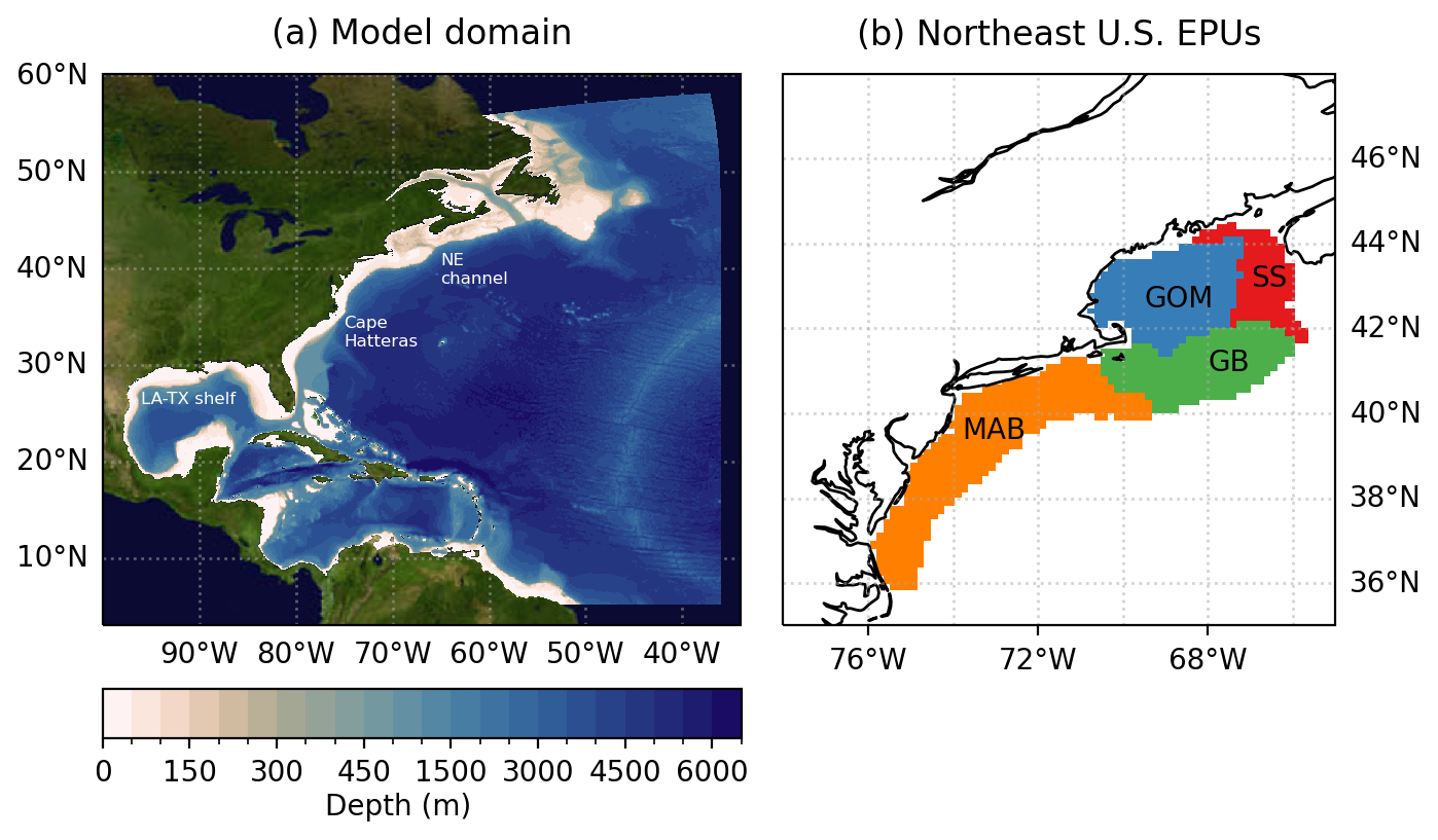
Figure 1(a) Model domain and bathymetry. The color-scale spacing is more detailed in the first 500 m to show shallow bathymetric features on the shelves. Annotations are placed near three geographic features mentioned in the text. (b) Northeast US ecological production units (EPUs) used for some model evaluation metrics: Scotian Shelf–eastern Gulf of Maine (SS), Gulf of Maine (GOM), Georges Bank (GB), and Mid-Atlantic Bight (MAB).
Confidence in the intended applications is linked to the model's capacity to accurately simulate past observed responses across these scales. Thus, in the sections that follow, we detail the development and configuration of the model components for a historical simulation covering 1993 to 2019, evaluate the ability of the model to reproduce the historical means of and variability in metrics with ecosystem relevance, and discuss several notable sensitivities that we identified during model development. Finally, we emphasize that the configuration herein is intended as an open development baseline supporting sustained model improvement. We thus conclude with a discussion of model strengths and limitations, with an eye toward future improvements, and a long-term goal of supporting climate-informed decisions across LMR management and decision-making time horizons from seasons to multiple decades.
MOM6-COBALT-NWA12 is comprised of coupled model components for ocean physics, ocean biogeochemistry, and sea ice. In this section, we detail the development and configuration of the regional model components and describe the configuration and evaluation of a reanalysis-forced simulation to determine whether the model is fit for purpose.
2.1 Physical ocean model configuration
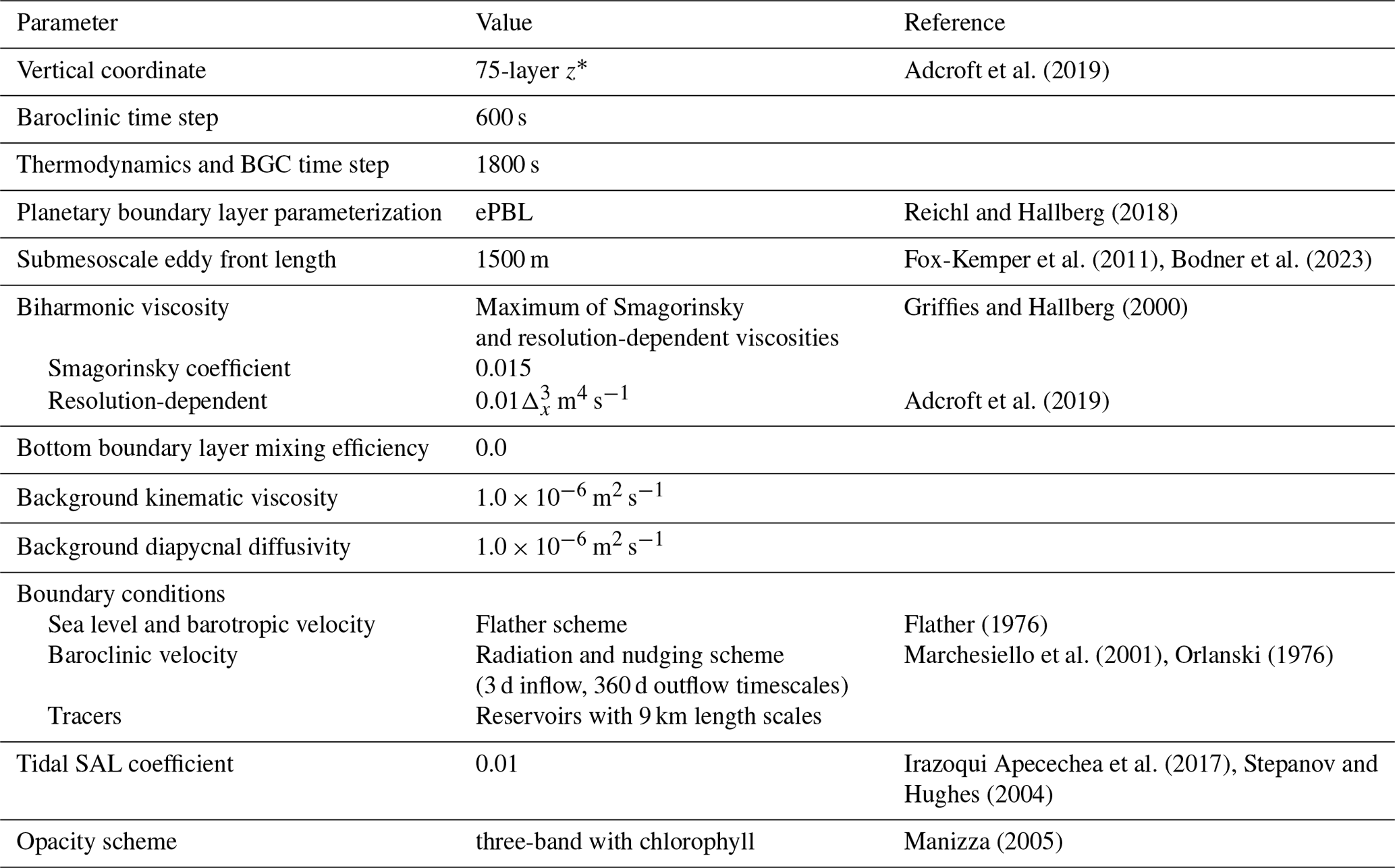
A summary of the main configuration choices used in the MOM6 component of the model is presented in Table 1. Horizontally, the model is based on an Arakawa C grid (Arakawa and Lamb, 1977) with 775×845 tracer points. The horizontal grid and bathymetry, shown in Fig. 1a, are extracted from the larger North Atlantic basin model of Xu et al. (2010), with open boundaries along the south, east, and north edges. Compared to a previous model based on the Regional Ocean Modeling System that was developed by several coauthors of this study (Kang and Curchitser, 2013, 2015) and applied to climate and ecosystem downscaling simulations (Alexander et al., 2020; Baumann et al., 2022; Clark et al., 2022), the NWA12 model domain is expanded to include the critical Grand Banks region in the northeast, cover the full Caribbean Sea including the coasts of Puerto Rico and the Virgin Islands, and generally place the open boundaries farther from coastal regions of interest. The resolution is ∘ throughout most of the domain, and the zonal distance between grid points varies primarily with latitude from approximately 9 km at the southern boundary to 5 km at the northern boundary. Vertically, the model uses a z∗ coordinate (a height coordinate that is rescaled with the free surface; Adcroft and Campin, 2004) with 75 layers and partial bottom cells, identical to the z∗-only configuration of the global OM4 model in Adcroft et al. (2019, hereafter A19) but different from the hybrid z∗-isopycnal configurations also developed in A19 and employed in GFDL's global climate and earth system models. The vertical resolution is finest near the surface, where the layer thickness is 2 m, and the layer thickness gradually increases with depth to a maximum thickness of 250 m above the deepest model depth of 6500 m. The shallowest bathymetry in the model is 10 m. The model is integrated forward in time with a split explicit method (Hallberg, 1997; Hallberg and Adcroft, 2009). The baroclinic time step is 600 s, and the time-varying barotropic time step is set to the largest integer fraction of the baroclinic time step that is less than 90 % of the maximum stable time step. To increase computational efficiency, we used MOM6's sub-cycled time-step capabilities to update the thermodynamics and biogeochemistry (BGC) on a slower 1800 s time step, and the atmospheric forcing data and external biogeochemical boundary data are updated hourly. The computational efficiency gained through these choices is discussed in the Results.
Adcroft et al. (2019)Reichl and Hallberg (2018)Fox-Kemper et al. (2011)Bodner et al. (2023)Griffies and Hallberg (2000)Adcroft et al. (2019)Flather (1976)Marchesiello et al. (2001)Orlanski (1976)Irazoqui Apecechea et al. (2017)Stepanov and Hughes (2004)Manizza (2005)Table 1Major parameters and associated values used in the physical ocean (MOM6) component of the model and relevant references describing the parameter or the choice of value. BGC denotes biogeochemistry; SAL denotes self-attraction and loading.
The ocean model subgrid-scale parameterizations are adapted from the ∘ global model of A19, with updates and modifications to account for the increased horizontal resolution and other differences in MOM6-COBALT-NWA12. The planetary boundary layer is parameterized using the same Reichl and Hallberg (2018) energetic planetary boundary layer scheme; however, the parameterization in NWA12 includes the updates by Reichl and Li (2019) to account for enhanced mixing by Langmuir turbulence. Since our resolution resolves the first baroclinic deformation radius across the majority of the model domain, except on the shelves (Hallberg, 2013), and thus captures a considerable fraction of the mesoscale dynamics, we did not include a mesoscale eddy mixing parameterization (nor did the ∘ configuration in A19). Restratification of the mixed layer by submesoscale eddies is parameterized using the scheme based on Fox-Kemper et al. (2011). As in A19, we found a strong sensitivity of the simulated mixed-layer depths to the submesoscale front length parameter in this scheme, and we increased the front length from 500 m in A19 (which is on the lower end of values typically used; Bodner et al., 2023) to 1500 m. This increased front length decreases restratification arising from the parameterization. Like A19, the horizontal biharmonic viscosity is formulated as the maximum of either a Smagorinsky viscosity or a fixed viscosity of the form , where Δx is the local grid spacing (Griffies and Hallberg, 2000). NWA12 uses u4=1 cm s−1, the same as A19, with a Smagorinsky coefficient of 0.015, which is reduced from 0.06 in A19. Mixing by shear-driven turbulence is modeled using the Jackson et al. (2008) parameterization as in A19.
There are a few other differences from A19. Most notably, MOM6-COBALT-NWA12 includes explicit tidal dynamics forced by both the boundary and the astronomical tidal potential. We thus removed the unresolved tidal velocity from the formulation of the bottom drag, and we did not include parameterized mixing or the additional tracer diffusivity that A19 used to account for internal tides. Background vertical viscosity was reduced to its molecular value. We also neglected the parameterized conversion of energy dissipated in the bottom boundary layer to diapycnal mixing by reducing the parameter for the efficiency of this process from 0.20 in A19 to 0.0. When this parameterization was enabled, the model tended to produce exaggerated mixing at the bottom of many coastal areas, which prevented the development of realistic bottom hypoxia in the coastal Gulf of Mexico. The efficiency is considered poorly constrained (generally within a range of 0.0–0.2) and tunable (Gregg et al., 2018; Legg et al., 2006), although eliminating this parameterization of physical mixing may partially compensate for numerically induced mixing in the z∗ coordinate model (Griffies et al., 2000).
As in A19, MOM6-COBALT-NWA12 simulates sea ice and its interaction with the ocean using a coupled sea ice model, Sea Ice Simulator version 2 (SIS2). We refer the reader to A19 for a description of the SIS2 model and configuration; the configuration used in MOM6-COBALT-NWA12 is identical except we have reduced the ice dynamics time step to 600 s to match the ocean baroclinic time step. SIS2 does not yet support open boundary conditions for sea ice.
2.1.1 Physical ocean model forcing
Boundary conditions for combined tidal and subtidal sea level and barotropic velocity are set using a Flather (1976) radiation boundary condition. Baroclinic flow at the boundary is set using the radiation scheme of Orlanski (1976) combined with nudging toward external forcing data following Marchesiello et al. (2001). Boundary normal and tangential velocities are strongly nudged toward the forcing data with a 3 d timescale for flow entering the model and weakly nudged with a 360 d timescale for outgoing flow. Temperature and salinity boundary conditions are set using a reservoir scheme that gradually adjusts boundary data toward interior values on outflow and exterior values on inflow, which allows the tracer boundary conditions to retain a memory of the properties of flow that exits and re-enters the domain. The reservoir length scale is set to 9 km for both inflow and outflow, which is approximately equal to a 1–10 d timescale for a 10–1 cm s−1 flow and allows the boundary to adjust to changes on weather timescales. The development of and sensitivity to this novel reservoir scheme are being addressed in a separate publication. For all prognostic model variables there is no nudging to observed data within the model domain – the model does not use a “sponge layer” near the boundary or apply restoring of properties like surface salinity. Attaining a reliable solution without using these features was an emphasis of model development and facilitates use of the model in downscaled climate projections and other scenarios where accurate internal data to restore to may not be available (it will, however, be necessary to confirm that the model remains reliable over simulations longer than the 27-year run examined here).
In the reanalysis-driven hindcast simulation presented in this paper, external boundary data for temperature, salinity, and subtidal velocity and sea level were specified using daily averages from the GLORYS12 v1 ocean reanalysis (Lellouche et al., 2021). This reanalysis provides high-resolution (∘) daily data and has been found to be one of the better-performing ocean reanalyses in coastal areas including the northeast USA (Carolina Castillo-Trujillo et al., 2023) and California current system (Amaya et al., 2023). Tidal variations in sea level and velocity were superimposed on the subtidal boundary data using tidal harmonics from the TPXO9 v1 dataset (Egbert and Erofeeva, 2002). Four semidiurnal constituents (M2, S2, N2, and K2), four diurnal constituents (K1, O1, P1, and Q1), and two long-period constituents (Mm and Mf) were included in the boundary forcing. Modulation by the 18.6-year nodal cycle was included by calculating correction factors for the amplitude and phase of each constituent at yearly intervals. Astronomical tidal forcing from the same 10 constituents was also included throughout the domain as a body force in the momentum equations. The effects of self-attraction and loading were also included using the scalar approximation (Accad and Pekeris, 1978) with a coefficient of 0.01.
Freshwater discharge from rivers was sourced from the gridded daily GloFAS reanalysis version 3.1 (Alfieri et al., 2020). River discharge was mapped to the MOM6 grid using the local drainage direction map to identify outlet points adjacent to the coast and any chains of outlet points adjacent to these coastal outlets, and the streamflow at each outlet point was mapped to the nearest MOM6 coastal ocean grid cell. River discharge was added at the surface at the discharge grid cells, and an additional source of turbulent kinetic energy was added at discharge points to vertically mix the water column up to 5 m deep. River discharge entered with zero salinity and a temperature equal to the surface temperature of the discharge grid cell. We found that the GloFAS product overestimated the streamflow in the Mississippi River, so we applied a bias correction using a linear regression between the GloFAS Mississippi River discharge and the United States Geological Survey (USGS) gauge at Belle Chasse, LA. We evenly divided this adjusted flow into two points that discharged on the western side of the river delta and one point on the eastern side, which is roughly consistent with the real partitioning of discharge from the delta (Dagg and Breed, 2003; Dinnel and Wiseman, 1986). River discharge from the Atchafalaya River did not appear to need adjustment. We also manually adjusted the location of discharge from the Susquehanna River to ensure that it entered the model at the correct location in Chesapeake Bay.
Momentum, heat, freshwater, and radiation fluxes between the ocean and atmosphere were calculated using the hourly ERA5 atmospheric reanalysis (Hersbach et al., 2020) and the Large and Yeager (2004) bulk algorithm, with the inclusion of the Large and Yeager (2004) adjustment for the temperature and humidity reference height of 2 m in the ERA5 data. Chlorophyll predicted by the coupled COBALT biogeochemical component of the model, presented next, was used to specify the vertical profile of the absorption of shortwave radiation following the Manizza (2005) scheme.
2.2 Biogeochemical model configuration
The MOM6 physical ocean component is coupled with the Carbon, Ocean Biogeochemistry and Lower Trophics (COBALT) biogeochemical model (Stock et al., 2014, 2020), with a number of enhancements intended to improve the robustness of the biogeochemical model across the spectrum of coastal to open-ocean environments included in the NWA12 domain. For the plankton food web, we drew from Van Oostende et al. (2018) to add a fourth phytoplankton group to better represent spring bloom diatoms that can be particularly prominent in high-productivity coastal regions. The phytoplankton parameters enlisted in this run are summarized in Table A1. Direct phytoplankton sinking was added to complement phytoplankton aggregation losses under poor growth conditions and better capture the absence of large diatoms in the subtropical gyres. Upon reaching the bottom, these slowly sinking particles were assumed to settle into a nepheloid layer and be available for resuspension if the bottom was shallower than twice the depth of the actively mixed layer, and they were otherwise remineralized. Other aspects of particle sinking and remineralization are as described in Stock et al. (2020).
Phytoplankton in very deep mixed layers (those exceeding three e-folding depths) were assumed to photoacclimate to mean light levels over the first three e-folding depths, while those in shallow mixed layers were assumed to photoacclimate to mean light levels over the mixed layer. This is consistent with results of optimality models suggesting that phytoplankton in deep mixed layers must adapt to elevated light conditions closer to the surface (Talmy et al., 2013) and was found to improve the model's representation of offshore bloom timing and magnitude in the NWA12 domain.
Increased flexibility was added to the zooplankton grazing kernels to better represent the feeding flexibility of the diverse groups included within COBALT's three zooplankton size classes (Fuchs and Franks, 2010; Hansen et al., 1994). The prey availability is summarized in Table A2. In accordance with Van Oostende et al. (2018), grazing of the largest phytoplankton size class was limited primarily to the largest zooplankton (i.e., large-bodied copepods and krill), with only weak controls by medium-sized zooplankton. More flexibility was allotted across the smaller size classes.
To better represent light limitation in nearshore waters and/or waters under strong riverine influence, we enhanced the light attenuation in waters with salinity < 30 PSU or depth < 30 m to levels consistent with case-2 waters (Jerlov, 1976). This was achieved by augmenting the background light attenuation in the Manizza (2005) scheme by 0.05 m−1. This yields blue–green diffuse attenuation rates of about 0.1–0.3 m−1 (transmittance of 90 % m−1 to 75 % m−1) for typical coastal chlorophyll levels between 0.5 and 5 mg chl m−3, respectively. This augmentation to the light attenuation is currently only active for photosynthetic calculations in the biogeochemical model and is acknowledged to be a simple first step toward more comprehensive representations of complex coastal ocean optics (e.g., Skákala et al., 2020). Its inclusion reflects the potential importance of the depth of the euphotic zone for hypoxia in the Gulf of Mexico (Schaeffer et al., 2011).
To allow COBALT to better integrate riverine nutrient inputs that have nitrogen-to-phosphorus ratios (N:P) that often strongly depart from characteristic oceanic (i.e., Redfield) values, we augmented the phytoplankton N:P ratios for small, medium, and large phytoplankton to include the potential for reduced P usage in low-P environments (i.e., “P frugality”). This was parameterized with the emergent negative relationship between phytoplankton N:P and P concentration identified by Galbraith and Martiny (2015), enabling phytoplankton to achieve a maximum N:P ratio of 31 (nearly twice the canonical Redfield ratio) in low-P environments. Minimum N:P ratios were restricted to characteristic values for each size class (Finkel et al., 2010) because the highest-P regions in the NWA12 are generally associated with high N:P riverine inputs, which observations (e.g., Sterner and Elser, 2003; Hall et al., 2005) suggest would prevent the lower N:P ratios predicted by the Galbraith and Martiny (2015) relationship under phosphate-rich conditions. The net effect of this simple phytoplankton N:P parameterization is thus to allow phytoplankton to better utilize excess N under low-phosphate conditions, while reverting to characteristic N:P ratios under moderate and high phosphate levels. The addition of the fourth phytoplankton group and dynamic phytoplankton N:P ratios increases the number of prognostic state variables in COBALT from 33 in its standard formulation to 40.
2.2.1 Biogeochemical model forcing
Open boundary data for biogeochemical tracers were set using several sources. Boundary data for NO3, O2, PO4, and SiO4 were obtained from climatologies in the World Ocean Atlas (WOA) 2018 dataset (Boyer et al., 2019). In the upper 800 m, we used seasonal climatologies from the WOA as boundary conditions, while below 800 m (where only long-term mean values are available) we used the long-term mean data. Boundary data for alkalinity (ALK) and dissolved inorganic carbon (DIC) were estimated from GLORYS monthly average temperature and salinity by applying the methods developed by Carter et al. (2021). We used the multiple linear regression version of the algorithm from Carter et al. (2021) that predicts ALK and DIC from potential temperature and salinity using a multiple linear regression, with an adjustment for the year. Carter et al. (2021) fit parameters for the regression over a depth grid, and these coefficients were then interpolated to the NWA12 model boundaries and used to predict time-varying ALK and DIC from the interpolated GLORYS12 temperature and salinity. Boundary data for the remaining tracers, which generally have shorter turnover times, were set to 1993–2014 averages from the global COBALT simulation of Stock et al. (2014).
Biogeochemical tracers used the same tracer reservoir boundary condition scheme as temperature and salinity. However, as the external biogeochemical fields are not as well constrained by data as temperature and salinity and biogeochemical simulations are sensitive to even small amounts of spurious mixing or circulation near the boundary, we increased the inflow length scale to 300 km. This succeeded in imposing the desired lower-frequency biogeochemical trends at monthly and longer timescales while approaching a no-gradient condition for dynamics operating on daily timescales within the euphotic zone, thus dampening spurious biogeochemical signals. The impacts from such signals are further dampened by the large distance between the domain boundaries and the coastal regions of primary interest.
The primary source of river nutrient, carbon, and alkalinity data was the River Chemistry for the United States Coast (RC4USCoast) dataset compiled by Gomez et al. (2023). This product relies mainly on river chemistry observations from the USGS sub-selected for inputs to coastal waters and processed into monthly climatologies and, where possible, time series. The simulations herein used the 1990–2022 climatology to constrain dissolved organic carbon (DIC), alkalinity (ALK), nitrate (NO3), ammonia (NH4), phosphate (PO4), the dissolved and particulate organic phases of N and P, oxygen (O2), and silicate (SiO4, derived from data on silicon dioxide, SiO2). Of particulate phosphorus, 50 % was assumed to be mobilized in estuaries, with the remainder buried (Froelich, 1988; Sutula et al., 2004). Dissolved organic nitrogen and phosphorus inputs were fractionated to labile (40 %), semi-labile (30 %), and semi-refractory (30 %) pools to be consistent with the range of bioavailability in Wiegner et al. (2006).
For Canadian waters, the river forcing described in Lavoie et al. (2021) was enlisted. These data included DIC, ALK, and nitrate. Other nutrient inputs were estimated by applying the ratios between dissolved inorganic nitrogen and PO4 and dissolved and particulate N and P from the semi-empirical GlobalNEWS2 algorithm (Mayorga et al., 2010) to the Lavoie et al. (2021) nitrate estimates. GlobalNEWS2 estimates were enlisted directly to constrain river inputs in Mexico and Central and South America. Oxygen for Canadian and Mexican–Central American–South American rivers was specified to be in equilibrium with climatological ocean temperatures at the river mouths. Following de Baar and de Jong (2001), iron concentrations in all rivers were specified to be 70 nM.
RC4USCoast and other nutrient concentrations were mapped onto GloFAS freshwater inputs (see Sect. 2.1) using a nearest-neighbor algorithm with larger rivers superseding smaller ones. Nutrient loads vary with river flows and month, but more subtle variations/trends in nutrient concentrations over the 1993–2019 model simulation period (e.g., increasing alkalinity in the Mississippi–Atchafalaya river system; Gomez et al., 2021) are omitted for the baseline configuration presented herein.
For the atmosphere, time- and latitude-varying atmospheric CO2 concentration was set using the monthly historical time series from Meinshausen et al. (2017). We extended the historical CO2 time series, which ends in 2014, using the atmospheric CO2 concentration projected under the SSP2-4.5 emissions scenario (Meinshausen et al., 2020). Wet and dry deposition of NO3, NH4, and lithogenic dust was specified using a 1993–2014 monthly climatology from the historical simulation of GFDL's ESM4.1 earth system model (Dunne et al., 2020). As in ESM4.1 (Stock et al., 2020), iron deposition was approximated by assuming that dust is composed of 3.5 % iron and iron solubility varies inversely with the surface dust concentration following Baker and Croot (2010). Dry deposition of phosphorus was also approximated from the climatology of dry dust deposition by assuming that dust consists of 563 ppm phosphorus of which 22 % is bioavailable. These values were obtained from the global ocean averages of Herbert et al. (2018).
2.3 Model spinup and hindcast simulation
The primary model simulation evaluated in this paper is a hindcast simulation that was run from 1993 to 2019 using the configuration and forcing described in previous sections. This simulation was initialized from rest on 1 January 1993. The ocean temperature and salinity were initialized by directly using GLORYS12 temperature and salinity for that date rather than starting from a previously run spinup simulation. During model development, we found that spinning up the physics first, by repeating either the first year or the first 10 years, produced less reliable initial conditions than the high-resolution GLORYS12 reanalysis and led to substantial errors in the beginning of the simulation. For the biogeochemical tracers, however, we ran a 10-year spinup beforehand to allow the biogeochemistry to adjust from the coarse climatological initial conditions, at least near the surface. This spinup simulation also started from rest in 1993 using initial conditions from the GLORYS12 reanalysis and the same biogeochemical data sources used to create the boundary conditions. We ran this simulation for 10 years using 1993–2002 time series of forcings described previously. Carbon dioxide forcing was applied differently during this spinup simulation, however, to obtain a model state closer to equilibrium with 1993 conditions: atmospheric CO2 was applied by repeating the 1993 annual cycle from the Meinshausen et al. (2017) forcing dataset, and open-boundary-condition ALK and DIC were calculated using the Carter et al. (2021) algorithm with the time fixed to 1993. We then started the main hindcast simulation on 1 January 1993 using the biogeochemical tracer fields at the end of the spinup simulation as initial conditions for the main simulation.
2.4 Model evaluation
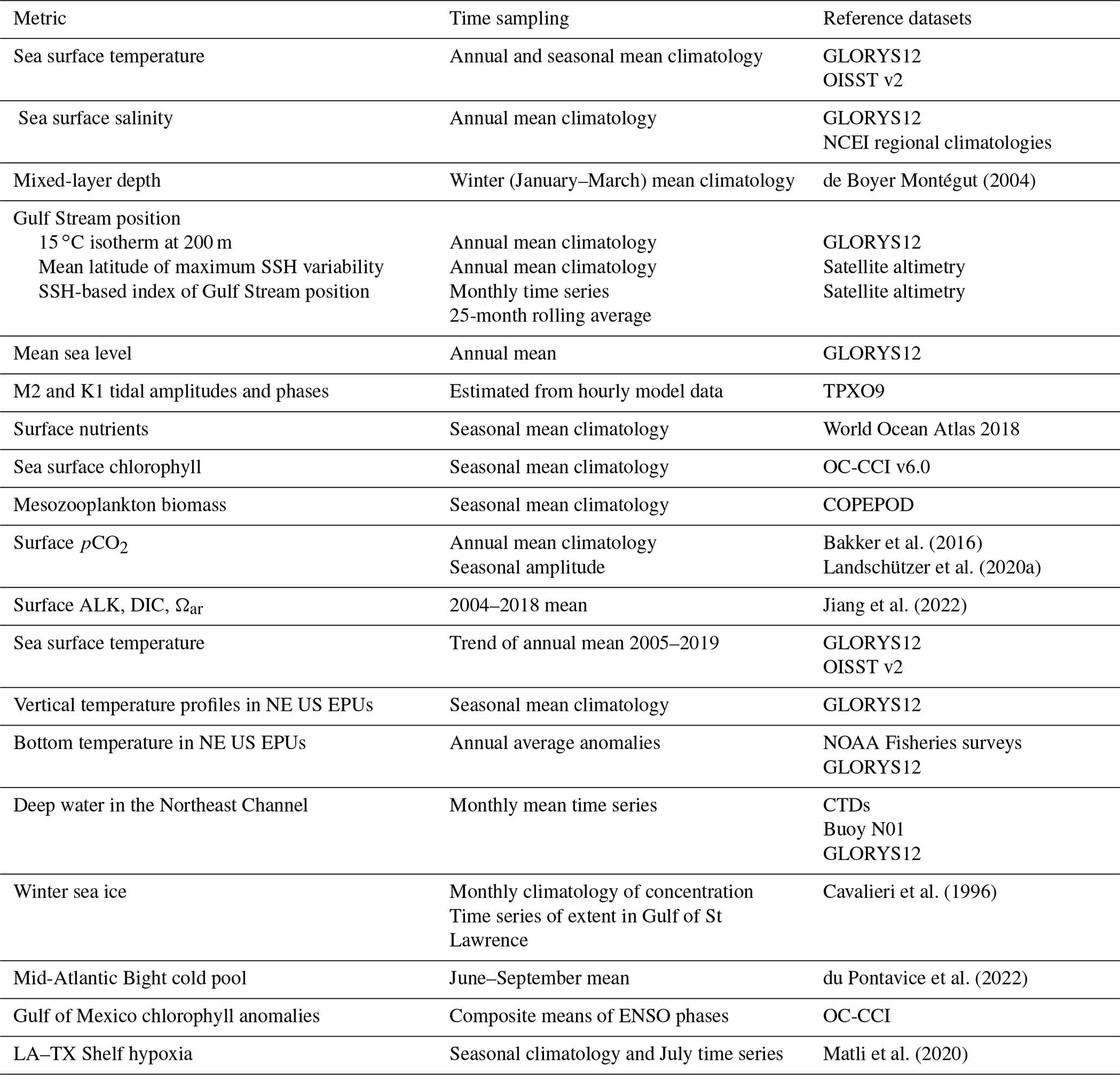
To evaluate the utility of the NWA12 model for marine resource applications, we focused on three aspects of the model performance. First, we considered general, basin-wide indicators of the model simulation fidelity, such as climatologies of surface temperature and macronutrients, and drivers of large-scale variability, such as the mean of and variability in the position of the Gulf Stream. Second, we evaluated a high-priority subset of features that are essential to simulate accurately in order to reproduce regional ecosystem variability, such as the temperature and salinity of water entering the Gulf of Maine at depth through the Northeast Channel, and fine-scale ecosystem responses to climate variability, such as hypoxia on the Louisiana–Texas Shelf. For these two sets of model–data comparisons, a summary of the metrics considered and the datasets used as references is provided in Table 2. Third, we tested the computational cost and scaling of the model to assess the feasibility of using the model to run the long hindcasts and multi-member forecasts and projections needed to inform living-marine-resource management and other applications to coastal ocean decision-making.
de Boyer Montégut (2004)Bakker et al. (2016)Landschützer et al. (2020a)Jiang et al. (2022)Cavalieri et al. (1996)du Pontavice et al. (2022)Matli et al. (2020)Table 2Primary diagnostics used to evaluate the model, the time sampling of these diagnostics, and datasets used as references for evaluation of model performance. SSH denotes sea surface height; ENSO denotes El Niño–Southern Oscillation.
Most physical ocean metrics were evaluated using the GLORYS12 reanalysis, which was also used as the model open boundary conditions and reliably simulates regional hydrography (Carolina Castillo-Trujillo et al., 2023), as a reference dataset. We also included results from one or more in situ or remote sensing observational datasets as an additional comparison where available. For most model–data comparisons, we calculated four quantitative skill metrics: bias (mean difference between model and data), root mean square error (RMSE), Pearson correlation coefficient (corr., or r), and median absolute error (MedAE, expressed as , which is robust against outlying errors). For chlorophyll, we used the Spearman rank correlation instead of the Pearson correlation due to the nonlinearity of the data. All of these metrics were calculated using the xskillscore Python module (https://doi.org/10.5281/zenodo.5173153, Bell et al., 2021). For spatial comparisons where the observed product had a similar resolution to the NWA12 model grid (finer than ∘), the observations were bilinearly interpolated onto the model grid. One exception is chlorophyll a, which has fine resolution in the observed product (4 km) and high spatial variability and thus was interpolated onto the NWA12 model grid with a method that preserved the geometric mean chlorophyll. For spatial comparisons where the observed product had a resolution of ∘ or coarser, the model data were interpolated onto the observed product grid with a first-order conservative method. All comparisons except for the tidal sea surface height evaluation used monthly mean model output or longer-period averages calculated from monthly or daily means, so no processing was applied to remove tides from the model output.
2.4.1 Basin-wide indicators of model performance and drivers of variability
Model mean sea surface temperature (SST) was compared with the means of the ∘ OISST v2 product derived from remote sensing and in situ observations (Reynolds et al., 2007) and the GLORYS12 reanalysis. We compared the difference between the 1993–2019 model mean and the same time period from the two reference datasets. We also evaluated model biases in the seasonal SST climatology by comparing this metric to the OISST product.
We compared the 1993–2019 mean sea surface salinity (SSS) from the model with the corresponding mean SSS from the GLORYS12 reanalysis and from the NOAA National Centers for Environmental Prediction (NCEI) regional ocean climatologies, which are interpolated and quality-controlled climatologies at ∘ resolution derived from the World Ocean Database (Seidov et al., 2018, 2019). For the NCEI regional climatologies, which are provided as decadal averages with the most recent decade extended to 2017, we used the weighted average of the 1995–2004 and 2005–2017 means.
MOM6 computed the model mixed-layer depth (MLD) online using the common definition of the mixed-layer bottom as the depth where the potential density difference relative to the surface first reaches 0.03 kg m−3 (Griffies et al., 2016). We compared the winter (January, February, March) mean MLD with the long-term MLD climatology derived from profiles in the World Ocean Database and Argo datasets by de Boyer Montégut (2004). We used the November 2022 update to this dataset (https://doi.org/10.17882/91774, de Boyer Montégut, 2023). The MLD in this dataset is also defined as the depth where the density is 0.03 kg m−3 greater than the surface density; however, it uses 10 m depth as the surface, whereas MOM6 uses the surface layer (between 0–2 m here). On average this will introduce a small shallow bias into the model MLD relative to the de Boyer Montégut (2004) MLD when the model mixed-layer threshold is near or above 10 m or the diurnal cycle of 0–2 m temperature is large; however, as we examine only mixed layers during winter, when mixing is deeper and the diurnal cycle is weaker, the difference should be negligible.
The mean of and variability in the Gulf Stream position were calculated using two different metrics, one using temperature and the other using sea surface height (SSH). First, we calculated the position of the north wall of the Gulf Stream based on the position of the 15 ∘C isotherm at 200 m depth in the 1993–2019 mean temperature (Chi et al., 2019; Fuglister and Voorhis, 1965). This metric was also calculated using the GLORYS12 reanalysis for comparison. Second, along meridional lines between 72 and 52∘ W spaced 1∘ in longitude apart, we calculated the latitudes where the variance of the monthly mean sea surface height anomaly (the difference between the monthly mean SSH and the 1993–2019 calendar month mean) was highest. These latitude–longitude points form the mean position of the Gulf Stream. An index representing north/south shifts of the Gulf Stream over time was calculated by averaging the sea level anomaly at the mean Gulf Stream position points and then dividing it by the standard deviation of the average sea level anomaly. Although short-term eddy variability will introduce some noise into this metric, longer-term means generally represent broad, coherent shifts in the Gulf Stream position, and thus we also calculated a 25-month centered rolling average of the index. These metrics for SSH-based mean position and variability are adapted from Pérez-Hernández and Joyce (2014) and are the same as those used in the NOAA Fisheries State of the Ecosystem (SOE) Report for the mid-Atlantic (NOAA Fisheries, 2022a). This metric was also calculated using monthly mean absolute dynamic topography from the gridded satellite altimetry dataset provided by the Copernicus Marine Service (https://doi.org/10.48670/moi-00148, Global Ocean Gridded L4 Sea Surface Heights And Derived Variables Reprocessed 1993 Ongoing, 2023). We also compared long-term mean sea surface height in the broader western boundary current region using the GLORYS12 reanalysis. The reanalysis assimilates satellite altimetry data and has a nearly identical long-term mean, aside from an apparent offset in the reference level.
The model simulation of tidal elevations was assessed by calculating the amplitudes and phases of the largest semidiurnal (M2) and diurnal (K1) constituents for each model grid point from hourly model output. Due to the computational time and storage costs of saving hourly model output, this assessment was only done for 1 year of model simulation started in 1993 with the same initial conditions as the main hindcast. This simulation also did not include the COBALT biogeochemical component to reduce the computational cost. Modulation of the tides by the 18.6-year nodal cycle was also disabled for this run so that the modulation did not need to be re-estimated and corrected for when calculating tidal constituents properties from the model output. The amplitudes and phases of the M2 and K1 constituents were calculated at every grid point in the model using the UTide Python package (Codiga, 2011; https://github.com/wesleybowman/UTide, last access: 20 May 2020) and were compared with corresponding amplitudes and phases from the TPXO tide data used as tidal boundary conditions in the NWA12 model.
Model-predicted surface chlorophyll a (chl a) was compared with satellite remote sensing estimates from the OceanColour Climate Change Initiative (OC-CCI) dataset version 6.0 (Sathyendranath et al., 2019), which merges estimates of ocean surface chl a from multiple satellites and algorithms into one consistent product. We compared the model and OC-CCI seasonal climatologies calculated over 1998–2019.
The model seasonal mean climatology of mesozooplankton biomass integrated over 0–200 m was compared with observations from the COPEPOD dataset (Moriarty and O'Brien, 2013). Mesozooplankton in the COBALT model consists of the medium (200–2000 µm equivalent spherical diameter, ESD) and large (2000–20 000 µm ESD) size classes. The COPEPOD dataset reports biomass that is adjusted to be consistent with measurements from a 333 µm mesh (Moriarty and O'Brien, 2013), which is likely to exclude a significant fraction of sizes on both the small and the large end of COBALT's zooplankton size range (Skjoldal et al., 2013). Shropshire et al. (2020), for example, found that mesozooplankton biomass in 333 µm mesh nets in the Gulf of Mexico was approximately half (0.5093) that measured in 202 µm mesh nets. This is similar to the 0.6195 adjustment found by O'Brien (2005), and Skjoldal et al. (2013) further suggest that an even smaller 150 µm mesh net would be better in coastal systems. Given these uncertainties, we multiplied COPEPOD biomass estimates by 2 before comparing them with COBALT. We recognize the possibility that escape by larger zooplankton size classes and inefficient net sampling of gelatinous zooplankton likely make the adjusted observations a lower bound for mesozooplankton biomass across the size range covered by COBALT.
Model seasonal surface nutrient climatologies were assessed by comparing modeled surface NO3 and PO4 with climatologies from the World Ocean Atlas (WOA) 2018 (Boyer et al., 2019). We used the seasonal climatologies from the WOA dataset, which use a different definition of the seasons (starting with January, February, March) than the standard meteorological seasons (starting with December, January, February) used in other analyses in this paper.
Model surface pCO2 was compared with observations derived from the Surface Ocean CO2 Atlas database version 2021 (SOCATv2021; Bakker et al., 2016) during 1993–2019 and against a pCO2 data product generated from SOCAT observations by a two-step neural network interpolation (data product; Landschützer et al., 2020a) during 1998–2015. We evaluated the model and observed seasonal variability in pCO2, which is expressed as the root mean square of the monthly pCO2 anomalies (rms, in µatm). Due to the discontinuous pCO2 observations in time in the SOCAT database, the evaluation of the model in reproducing the seasonal pCO2 variability was only performed against the data product.
Model surface total alkalinity, DIC, and the aragonite saturation state were compared with long-term observed means from the dataset of Jiang et al. (2022). This dataset applies an objective analysis technique to observations from the Coastal Ocean Data Analysis Product in North America (CODAP-NA; Jiang et al., 2021) and Global Ocean Data Analysis Project version 2 (GLODAPv2; Lauvset et al., 2021) to produce a 1∘ gridded long-term mean for each variable. The model means were calculated over the years 2004–2018 to match the time period of the observations from CODAP-NA.
2.4.2 Relevant regional features and ecosystem responses
Since the early 2000s, the ocean along the northeast United States has warmed faster than the vast majority of all other ocean regions (Pershing et al., 2015; Seidov et al., 2021). We assessed the ability of the model to reproduce this warming and other temperature trends throughout the model domain by calculating the 2005–2019 annual mean sea surface temperature trend at each point in the model and comparing this with trends from the GLORYS12 and OISST datasets used in Sect. 2.4.1. The year 2005 was chosen as the start date of the trend analysis to match the date chosen by Seidov et al. (2021) and is 1 year later than the date chosen by Pershing et al. (2015).
Next, we assessed four metrics related to subsurface temperature on the northeast US continental shelf: (1) subsurface temperature climatologies within four ecological production units (EPUs), (2) bottom temperatures averaged over the four EPUs, (3) deep temperature and salinity within the Gulf of Maine Northeast Channel and associated water masses, and (4) bottom temperature within the Mid-Atlantic Bight cold-pool region. All of these metrics except the first are used to inform management in the NOAA Fisheries State of the Ecosystem (SOE) reports for New England (NOAA Fisheries, 2022b) and the mid-Atlantic (NOAA Fisheries, 2022a). Observed data for these metrics were obtained directly from the SOE reports, and metrics from the model data were calculated using nearly identical methods.
New England and mid-Atlantic fishery management EPUs are defined for the southwestern Scotian Shelf–eastern Gulf of Maine, the Gulf of Maine, Georges Bank, and the Mid-Atlantic Bight (Fig. 1b). We evaluated two temperature diagnostics for these EPUs. The first diagnostic was vertical profiles of seasonal temperature climatologies. Using the model and the GLORYS12 reanalysis, the area-weighted average temperature within each EPU, in waters deeper than 60 m, was calculated for each season and each depth level up to 150 m. The second diagnostic was the time series of annual mean bottom-temperature anomalies. Within each EPU, area-weighted model average bottom temperatures were computed, and anomalies were calculated by subtracting the 1993–2010 monthly climatology for each EPU. For comparison, EPU-average bottom-temperature anomalies were extracted from the GLORYS12 reanalysis using identical methods. The model bottom-temperature anomalies were also compared with observations obtained directly from data used in the SOE reports. These observed anomalies were calculated using slightly different methods. Observed bottom temperatures were derived from CTD profiles collected during routine surveys that were performed at least twice per year (most often in the late-spring and autumn months). The annual harmonic method described in Mountain (1991), in which the climatology is a simple sine wave with a period of 1 year, was used to calculate these anomalies because it works well at extracting anomalies from these sparse and irregular data. Finally, for all three datasets, we calculated annual averages of the monthly anomalies.
Third, we assessed the model's ability to simulate water masses entering the narrow, deep Northeast Channel in the Gulf of Maine that drive ecosystem-relevant temperature and salinity variability within the gulf. Using methods from Mountain (2012) and the NOAA Fisheries State of the Ecosystem Report for New England (NOAA Fisheries, 2022b), we evaluated the model monthly mean potential temperature and salinity averaged in the channel between 42.2–42.6∘ N, 66.0–66.8∘ W, and 150–200 m depth. Temperature and salinity in the channel are influenced by mixing between relatively cool, fresh Scotian Shelf Water (defined by Mountain, 2012, as T=2 ∘C, S=32); moderately warm, salty Labrador Slope Water (T=6 ∘C, S=34.6); and very warm, salty Warm Slope Water (T=12 ∘C, S=35.4). Recent observations have shown a significant increase in Warm Slope Water and a corresponding decrease in Labrador Slope Water (Balch et al., 2022; NOAA Fisheries, 2022b), so we used annual mean potential temperature and salinity to calculate time series of the composition of the water in the channel in percentages of these two masses using methods from NOAA Fisheries (2022b). These metrics calculated from the model were compared with matching metrics determined using potential temperature and salinity from three different products: the database of CTD profiles used in NOAA Fisheries (2022b), the GLORYS12 reanalysis, and the N01 buoy from the Gulf of Maine Moored Buoy Program (Wallinga et al., 2003) (available at 180 m depth from June 2004–July 2017).
Fourth, the ability of the model to simulate the cool bottom water along the shelf that forms the Mid-Atlantic Bight cold pool was assessed by comparing June–September mean bottom temperatures in the model and GLORYS12 reanalysis and calculating the cold-pool index developed by du Pontavice et al. (2022) and reported in NOAA Fisheries (2022a). This index uses the June–September bottom-temperature anomaly averaged over a common cold-pool region defined by depth, average temperature, and latitude and longitude; see du Pontavice et al. (2022) for additional details. The index is higher when the bottom is warmer than average and the cold pool is smaller than average. The index was calculated by du Pontavice et al. (2022) using the GLORYS12 reanalysis from 1993–2019, and they extended the index farther back in time using a bias-corrected ocean model simulation. For historical context, we show the full time series; however, the du Pontavice et al. (2022) index is only derived from GLORYS12 during the time period when the model and data overlap.
The coastal ocean in the far northern portion of the model domain, including the Gulf of St Lawrence and the coast of Labrador and Newfoundland, partially freezes over in the winter. We assessed the ability of the coupled SIS2 sea ice model to simulate the spatial and temporal variability in sea ice cover in this region by comparing the model output with satellite observations of sea ice concentration from the National Snow and Ice Data Center (NSIDC) (dataset NSIDC-0051; Cavalieri et al., 1996). First, we compared the model and satellite monthly climatologies of sea ice concentration over 1993–2019. Second, we compared time series of the areal extent of sea ice in the Gulf of St Lawrence by determining the total area with a monthly sea ice concentration above 15 % for each month in the model and satellite data.
Moving the regional focus to the southern portion of the domain, the El Niño–Southern Oscillation (ENSO) has been shown to drive marine-resource-relevant variability in phytoplankton biomass in the Gulf of Mexico. Winters and springs when an El Niño occurs are associated with increased river discharge, stronger mixing, and changes in coastal currents, which tend to produce increased phytoplankton and surface chlorophyll in the northern Gulf of Mexico, while La Niña winters and springs show an opposite but weaker response (Gomez et al., 2019). We conducted an analysis similar to that of Gomez et al. (2019) to determine if the model could reproduce this mode of variability. We compared composite means of model surface chlorophyll during winter (December–February) and the following spring (March–May) in El Niño and La Niña years with composites calculated from the OC-CCI remote sensing estimates for the same years. El Niño events were defined as those where the 3-month running-average SST anomaly in the Niño-3.4 region, published as the ONI (Oceanic Niño Index) by the NOAA Climate Prediction Center, exceeded 0.5 ∘C in December and remained positive in the following spring, and La Niña years were defined as those where ONI was below −0.5 ∘C in December and remained negative in the following spring. During the period where both the model and OC-CCI data are available (winter 1997–2019), six El Niño events occurred (1998, 2005, 2010, 2015, 2016, 2019) and nine La Niña events occurred (1999, 2000, 2001, 2006, 2008, 2009, 2011, 2012, 2018); note that the year of an event is defined here as the year following the occurrence of the December ENSO anomaly.
Finally, the area along the Louisiana–Texas Shelf with bottom hypoxia (bottom dissolved oxygen concentration below 2 mg L−1) was calculated from model daily mean bottom oxygen and compared with data from the geostatistical model of Matli et al. (2020) that combines observations, ocean model, and atmospheric data into a reliable estimate of hypoxic area. We integrated the model hypoxic area over the same region as Matli et al. (2020) (between 89.512–94.605∘ W and 28.219–29.717∘ N with a depth of 100 m or less). Model performance was assessed by comparing monthly climatologies of hypoxic area averaged over the years where the model and geostatistical estimates overlap (1993–2017) and by comparing the time series of monthly mean hypoxic volume for July (the normal peak month of hypoxic area).
2.4.3 Computational implementation and scaling
To determine the feasibility of using the model to provide future predictions and projections with information about uncertainty to support living-marine-resource applications, we assessed the total run time of the model relative to approximate values needed to support application needs and relative to the number of processing elements (PEs) used. The primary configuration of the model evaluated in this paper was run using a 50 × 50 layout, which divides the 775 × 845 model grid across a 50 × 50 grid of PEs, yielding a 16 × 17 chunk of the model domain on a typical PE. The MOM6 land masking feature, which eliminates PEs that do not contain any ocean points, was enabled, resulting in only 1646 PEs actually used (a savings of 34 %). To assess the scalability of the model across other layouts, we determined the time needed to run 1 year of simulation using layouts of 40 × 40, 50 × 50, 60 × 60, and 70 × 70 PEs (because the model domain is nearly square in terms of grid points, we only considered square decompositions). We focused on the total run time of the model, including the time needed for initialization, running the main loop, and writing output, since this time ultimately determines the computational tractability of the model. Each 1-year timing simulation was repeated three times, and the run times were averaged to obtain a more accurate result.
We also assessed the benefit of a key feature of MOM6: the ability to separate the time steps for the ocean barotropic and baroclinic dynamics from the time step for tracer advection, thermodynamics, mixing, and coupled ocean biogeochemistry. The “thermodynamics” time step for the latter set of processes can be run with a significantly longer time interval than the dynamics for computational speed. The basic model configuration presented in this paper uses an 1800 s thermodynamics time step and a 600 s baroclinic dynamics time step. We assessed the benefits of this configuration in terms of computational cost by repeating the 60 × 60 and 70 × 70 layout experiments discussed previously using a 600 s time step for both thermodynamics and baroclinic dynamics, with all other configuration options identical.
These timing simulations were run on NOAA's “Gaea” high-performance computing system using the c5 partition that has two 64-core AMD EPYC 7002 series CPUs per node. All model source code was compiled using “production” mode, which enables aggressive compiler optimizations. The model source code is archived at https://doi.org/10.5281/zenodo.7893349 (Ross et al., 2023b).
3.1 Basin-wide indicators of model performance and drivers of variability
The MOM6-COBALT-NWA12 model accurately simulates the broad patterns of mean sea surface temperature throughout the domain, with moderate biases that are most prominent in the vicinity of the Gulf Stream (Figs. 2–3). These biases include a region of warm SST concentrated along the shelf break from Cape Hatteras to the Grand Banks and a region of cool SST to the south. The strongest cool bias in the model is found east of the Grand Banks where the North Atlantic Current takes a northward turn, which is consistent with the effects of an underestimation of the eastward extension of the Gulf Stream and the northward turn of the current that is often seen in ocean models across a wide range of spatial resolutions (e.g., Bryan et al., 2007; Scaife et al., 2011; Sein et al., 2017). The cool bias in MOM6-COBALT-NWA12 is substantially less than the biases of over −5∘ found in ∘ and ∘ global climate models using a previous version of MOM, although some of the warm biases near the coast are greater (Saba et al., 2016). Outside of the western boundary current region, the model SST bias is generally minor. However, the SST biases are consistently negative between −0.5 and 0 ∘C, and the overall area-weighted mean bias is −0.23 ∘C compared to OISST. The spatial pattern of the model SST bias is consistent across seasons (Fig. 3); however, the magnitude of the bias is higher in winter and spring and lower in summer and autumn.
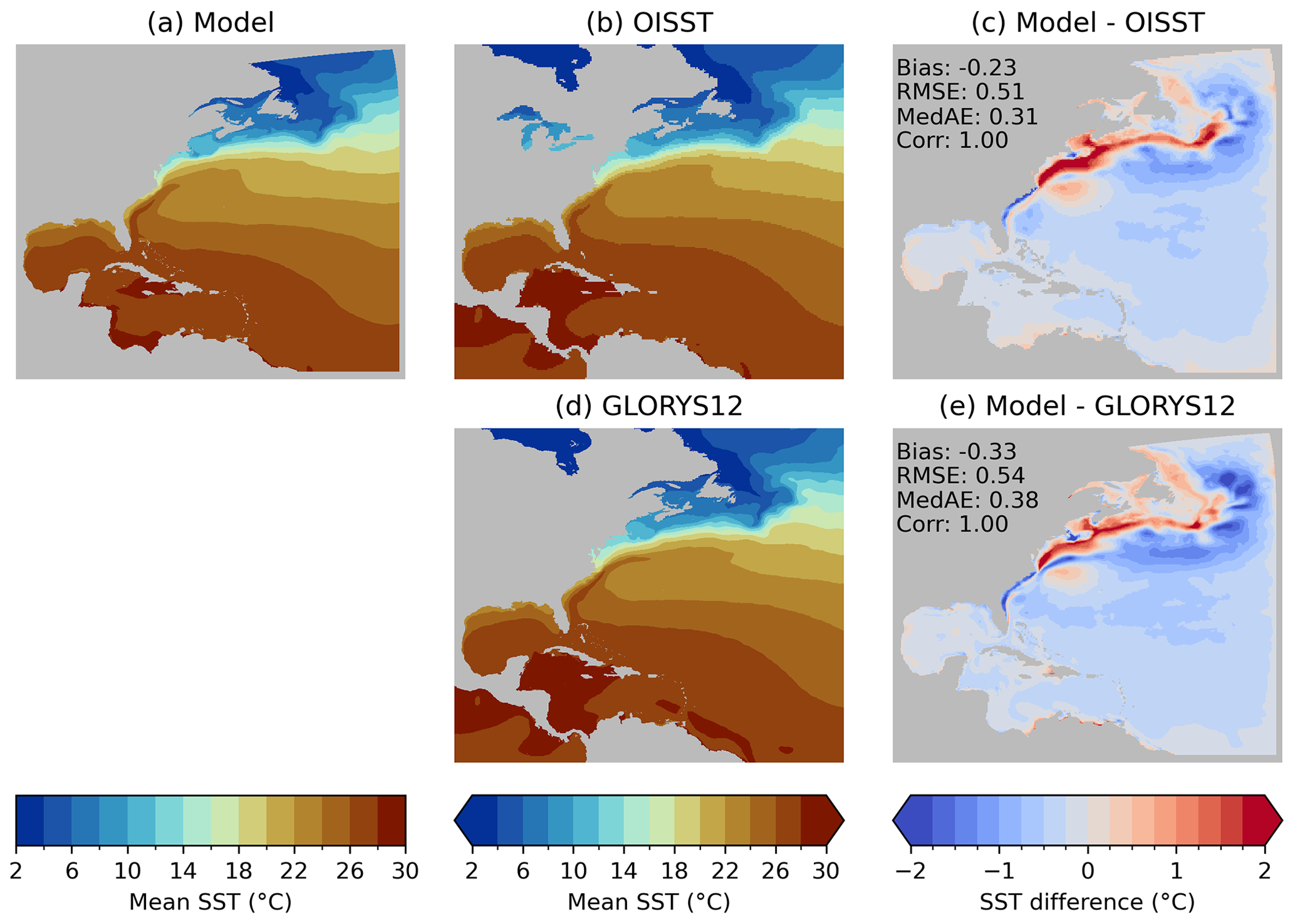
Figure 2The 1993–2019 mean sea surface temperature in the model (a) compared with the OISST (b) and GLORYS12 (d) datasets, and the difference between the model and the datasets (c, e).
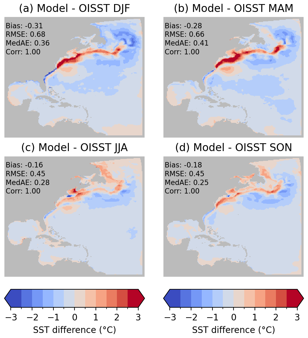
Figure 3Difference between the 1993–2019 seasonal mean sea surface temperature in the model and the OISST dataset.
In the patterns of model mean sea surface salinity and bias (Fig. 4), a positive surface salinity bias is present along the shelf from Cape Hatteras to the Gulf of St Lawrence, in the same region as the positive SST bias. The co-occurrence of these biases resembles, but is much milder than, the biases often seen in models with a poorly resolved Gulf Stream (e.g., Saba et al., 2016). Elsewhere in the domain, the patterns in the model bias suggest some errors in the volume and placement of rivers or in the river plumes and coastal currents that carry riverine freshwater. For example, model salinity is biased low to the west of the Mississippi River and high to the east. It is worth noting that at ∘, the model will not resolve the first Rossby radius of deformation along the coastal ocean where the rivers discharge (Hallberg, 2013; Piecuch et al., 2018), and this will limit the ability to capture the dynamics of the river plumes. Overall, the area-weighted model mean salinity is biased low by 0.27–0.28 units compared to the observational and reanalysis datasets.
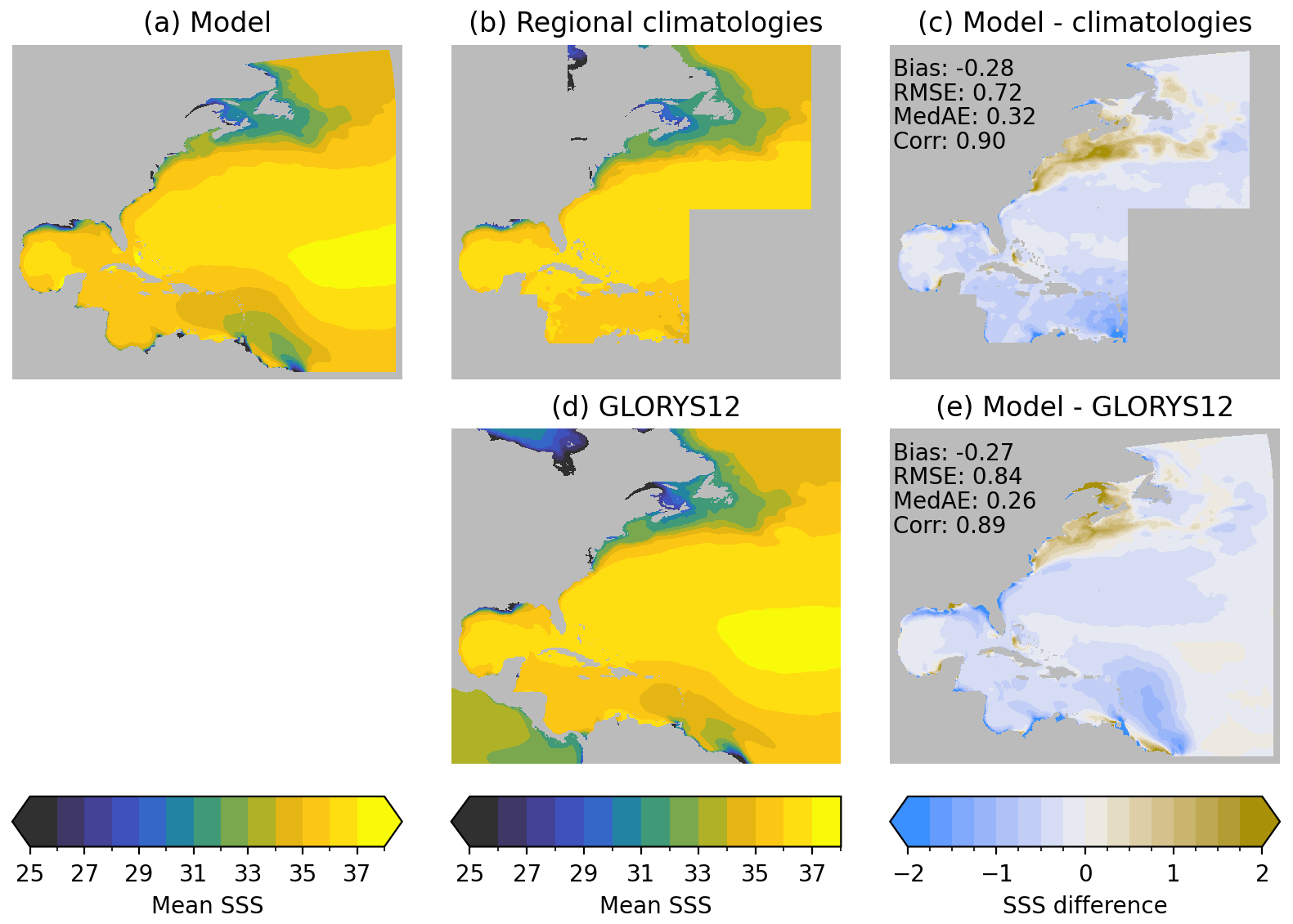
Figure 4The 1993–2019 mean sea surface salinity in the model (a) compared with the regional climatologies (b) and GLORYS12 (d) datasets, and the difference between the model and the datasets (c, e).
The model reproduces the broad patterns of winter mixed-layer depths when compared to estimates derived from profiles (Fig. 5). The spatial correlation coefficient for the mixed-layer depth based on a density difference from the surface of 0.03 kg m−3 is high (0.94), and the mean bias is negligible (0.90 m). The RMSE of 22.37 m is somewhat high relative to the typical value; however, the high correlation and low median absolute error of 8.02 m suggest the higher RMSE may be primarily due to mismatches in deep mixed layers. The model also has a tendency to predict winter mixed layers that are too deep to the north of the Gulf Stream along the shelf break, consistent with the temperature and salinity biases shown previously.
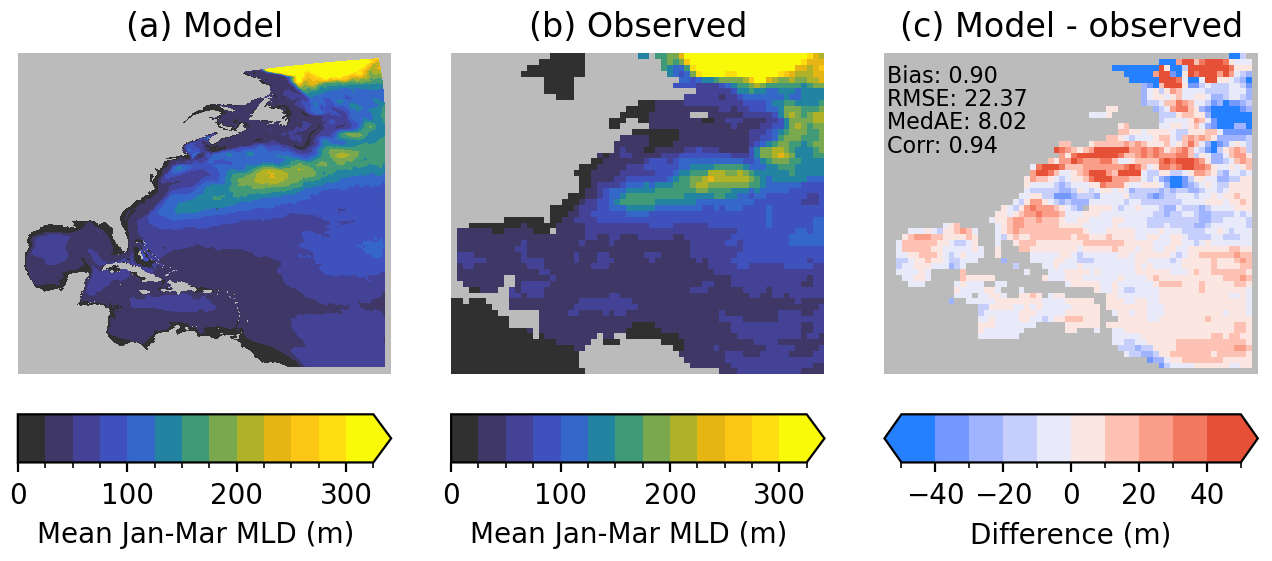
Figure 5Winter (January–March) mixed-layer depth in the model (a) and the observation-based climatology of de Boyer Montégut (2004) (b), and the difference between the two (c).
Although the previous metrics suggest the presence of a northward bias in the typical model Gulf Stream path, which would bring excessively warm and salty water to the northeast US shelf, both of the metrics for the position of the Gulf Stream show that the average position is remarkably close to observations (Fig. 6). The 15 ∘C isotherm of mean temperature at 200 m displays the canonical separation from the shelf at Cape Hatteras in both the model and GLORYS12 reanalysis (Fig. 6a). This metric actually suggests the presence of a slight southward bias in the Gulf Stream path of the model, particularly downstream of the separation, which is also seen in the metric based on SSH variance (Fig. 6b).
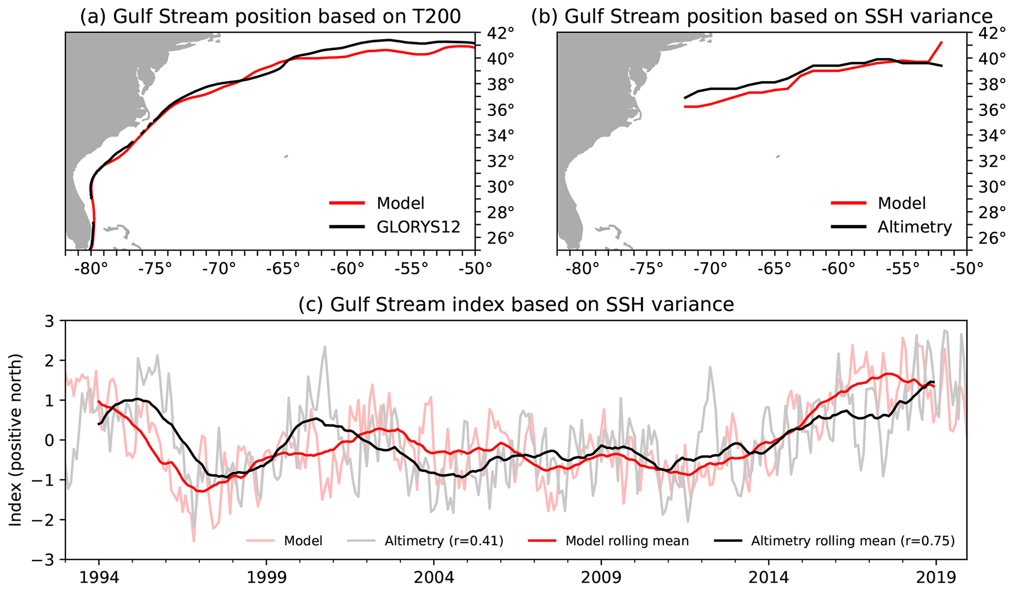
Figure 6Evaluation of model Gulf Stream position based on the 15 ∘C isotherm at 200 m (a) and the latitude of maximum sea surface height variance (b) and an index based on anomalies in the latitude of maximum SSH variance (c).
At low frequencies, north–south shifts in the position of the Gulf Stream are well simulated by the model, with a correlation of 0.75 for the 25-month rolling-mean Gulf Stream index (Fig. 6c). This simulation is particularly good considering that shifts in the Gulf Stream path are typically difficult to capture even in data-assimilative reanalysis products (Chi et al., 2018). The model accurately places the Gulf Stream farther south than usual (indicated by a negative index) in the late 1990s with anomalously northern positions in the early 1990s and 2000s. The modeled and observed position was relatively constant during 2006–2013. Finally, the model roughly reproduces the northward shift in the Gulf Stream that occurred starting around 2014, although the shift occurs faster in the model. At higher frequencies, fluctuations in the model-simulated position only loosely track the observed fluctuations associated with individual eddies and meanders – the correlation between the model and observations decreases from 0.75 for the 25-month rolling averages to 0.41 for the monthly values. However, this is not unexpected because the model boundaries are far from the region of interest and the model does not assimilate observations (i.e., eddies and meanders are present, but the formation and evolution of individual observed eddies are not deterministically simulated).
The spatial pattern of mean sea surface height in the northwest part of the model domain is consistent with Gulf Stream biases and the good performance in other parts of the domain (Fig. 7). Mean SSH closely resembles the reanalysis from the Loop Current through the Straits of Florida and up to Cape Hatteras. Beyond Cape Hatteras, the SSH pattern in the model has a weaker meridional gradient with more variability, the northwestern recirculation gyre (normally located offshore of the southern Mid-Atlantic Bight and visible as a region of low SSH) appears to be absent, and the Gulf Stream does not extend as strongly to the east and weakly curves to the north along the Grand Banks. These biases are consistent with the previous results: although the model simulates the mean of and low-frequency variability in the Gulf Stream path near the separation point well, the weaker and more variable extension, a weaker northwestern turn along the Grand Banks, and absent recirculation gyre combine to produce temperature and salinity biases with opposing patterns north and south of the mean Gulf Stream. Over the region shown in Fig. 7, the correlation between the model and the GLORYS12 reanalysis is high (0.97) and the errors are low (RMSE of 8 cm and median absolute error of 3 cm). The mean bias is also low (3 cm), which is expected given that the model is forced by the reanalysis at the boundaries.
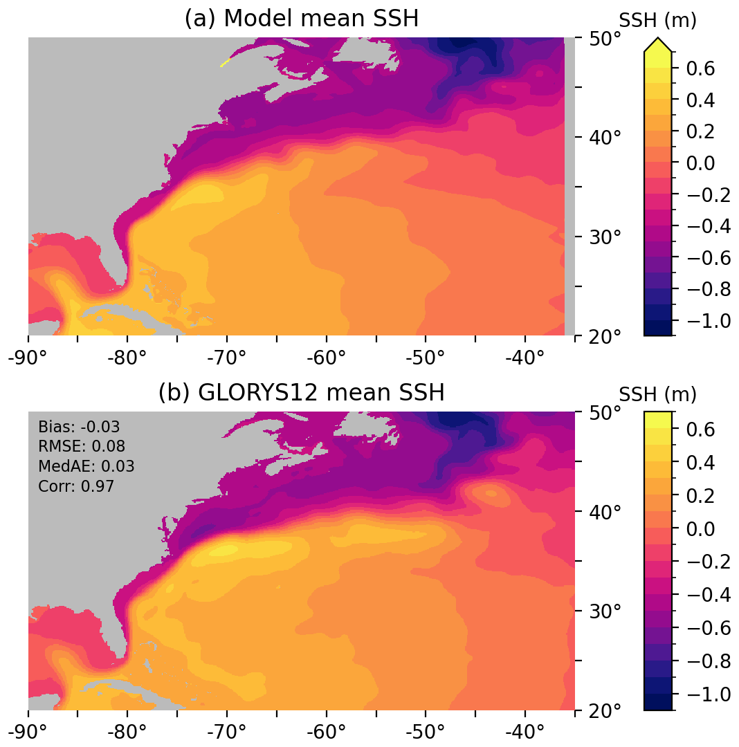
Figure 7The 1993–2019 mean sea surface height in the model (a) and the GLORYS12 reanalysis (b).
Semidiurnal and diurnal tides are well simulated in the model, with amplitude RMSEs that are low compared to the typical amplitude (RMSE of 5.44 cm for the semidiurnal M2 amplitude and 1.29 cm for the diurnal K1 amplitude) and high spatial correlations (0.95–0.96) (Figs. 8–9). Amplitude errors for the M2 tide are highest in the Gulf of Maine and Gulf of St Lawrence (Fig. 8). In the Gulf of Maine, the model M2 amplitude is too low in the Bay of Fundy and too high in the southwest portion of the gulf. M2 amplitudes are too high throughout the coastal Gulf of St Lawrence, although the central amphidrome (tidal node) is well placed in the model. The contour lines of the model M2 phase in the Caribbean Sea show a patchwork pattern. A closer look revealed a pattern of tidal amplitude similar to the surface expression of internal tides generated along the Windward Islands and in the passage between Puerto Rico and the Dominican Republic found by Zaron (2019) (not shown). For the diurnal K1 tide, the amplitude is also too high in the Gulf of St Lawrence and along the majority of the US East Coast and in the western Gulf of Mexico (Fig. 9). The phase of the model K1 tide is shifted by about an hour, particularly in the interior of the domain away from the boundaries.
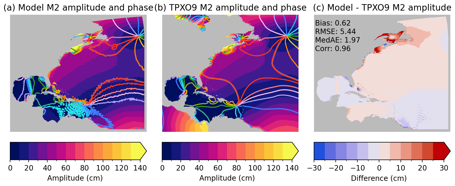
Figure 8Semidiurnal M2 tidal amplitude and phase estimated from hourly sea level output from the model (a) compared with the reference TPXO9 tidal model data (b) and the difference between the model and reference M2 amplitude (c). The phase in panels (a)–(b) is indicated by a differently colored line for each hour.
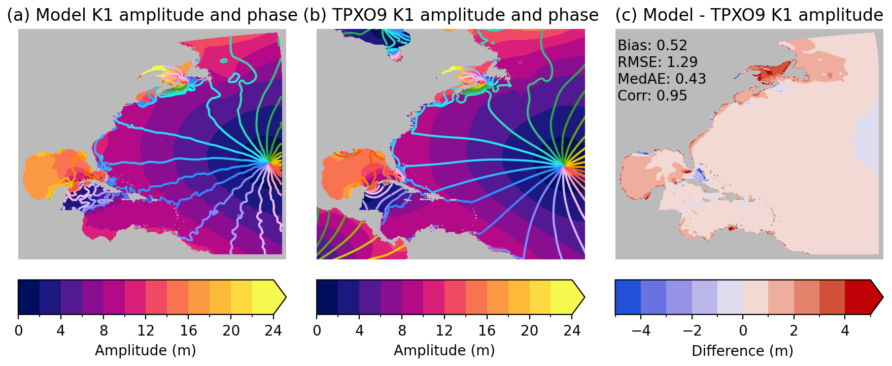
Figure 9Diurnal K1 tidal amplitude and phase estimated from hourly sea level output from the model (a) compared with the reference TPXO9 tidal model data (b) and the difference between the model and reference K1 amplitude (c). The phase in panels (a)–(b) is indicated by a differently colored line for each hour.
Shifting to biogeochemical patterns, the simulated surface nitrate (Fig. 10) and phosphate (Fig. 11) exhibit a robust large-scale nutrient drawdown from winter into the summer months. Winter nitrate, however, has a moderate high bias in shelf-adjacent waters in the northeastern part of the domain, aligned approximately with high MLD biases in this region (Fig. 5). This winter high bias delays the depletion of nitrate in the spring. The model and observations largely converge in the summer before high biases tend to re-emerge in the autumn with the onset of deeper mixing. Phosphate shows a similar winter/spring high bias to nitrate, as would be expected from a bias rooted in overly deep mixed layers along the shelf break. In contrast with nitrate, both the modeled phosphate and the observed phosphate remain elevated in summer months in the coastal waters of the northeast United States and Canada. Modeled phosphate, however, is somewhat lower than that observed. In the Gulf of Mexico, simulated summer phosphate surpluses are not as high as those that WOA suggests. The proximity of observed highs to some of the larger river systems in the southern Gulf of Mexico (e.g., Pánuco, Usumacinta, Coco) and Central and South America (e.g., Magdalena, Orinoco) suggests that part of this misfit may be attributable to uncertain river inputs in this region. In addition to the limited availability of river input data, ocean biogeochemical observations in the southern Gulf of Mexico are also sparse (Estrada-Allis et al., 2020), which introduces additional uncertainty into the comparison.
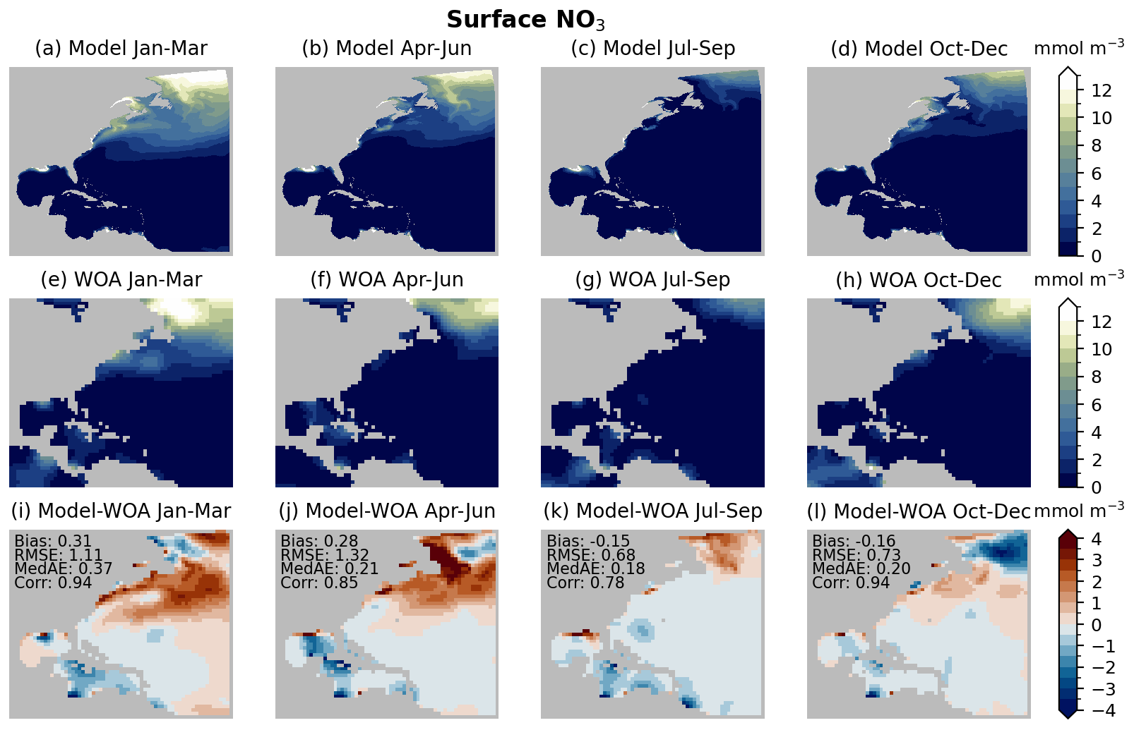
Figure 10Comparison of model seasonal mean surface nitrate (a, d, g, j) with the World Ocean Atlas (b, e, h, k) and the difference between the datasets (c, f, i, l).
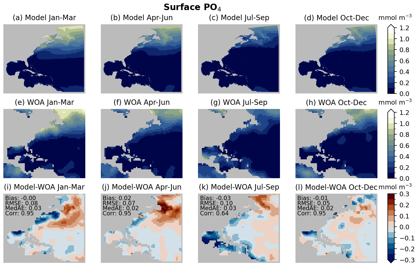
Figure 11Comparison of model seasonal mean surface phosphate (a, d, g, j) with the World Ocean Atlas (b, e, h, k) and the difference between the datasets (c, f, i, l).
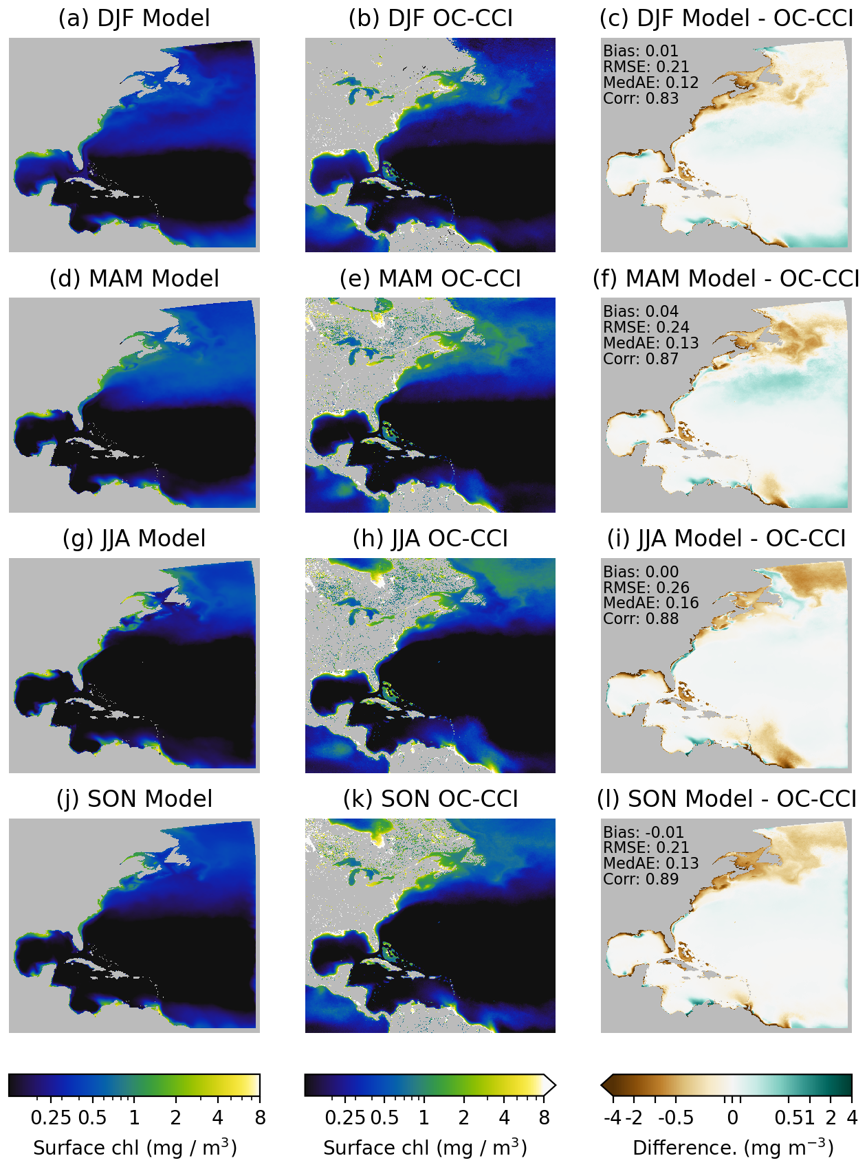
Figure 12Evaluation of model seasonal mean surface chl a (a, d, g, j) compared with OC-CCI satellite remote sensing estimates (b, e, h, k) and the difference between the datasets (c, f, i, l). Skill metrics were calculated for log 10-transformed chlorophyll. The color scale for the different panels is on a logarithmic scale except within ±0.1 mg m−3, where it is linear.
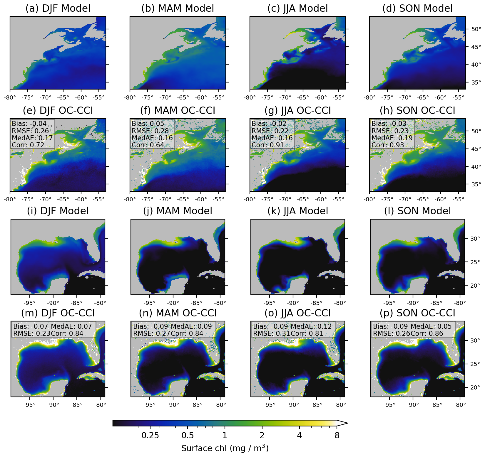
Figure 13A close-up of Fig. 12 for the northeast USA (a–h) and Gulf of Mexico (i–p). Skill metrics were calculated for log 10-transformed chlorophyll.
The mean seasonal patterns of surface chl a are simulated well by the model, despite some regional biases (Figs. 12–13). Spatial correlations (of log 10-transformed chlorophyll) between the model and OC-CCI remote sensing estimates range from 0.83 in winter to 0.89 in autumn, and RMSEs in log 10 units range from 0.21 in winter to 0.26 in summer, corresponding to a factor of 1.6–2.0 error. The chlorophyll minimum within the oligotrophic subtropical gyre is consistent with the satellite estimates, although chlorophyll is slightly higher than observed at the northern and southern limits of the gyre. Along the coast, in the northeast USA and Gulf of St Lawrence (Fig. 13a–h), seasonal patterns and cross-shore gradients are reproduced reasonably well, including the consistent chlorophyll hotspot on Georges Bank associated with sustained tidal mixing (Franks and Chen, 1996; Hu et al., 2008), the summer–autumn pattern of lower chlorophyll in the central Gulf of Maine ringed by higher chlorophyll along the coasts, high chlorophyll concentration in the lower St Lawrence Estuary and southern Gulf of St Lawrence, and a chlorophyll maximum that shifts from the spring in the Gulf of St Lawrence to summer in the estuary (Laliberté and Larouche, 2023). The correlation between the model and OC-CCI climatologies is highest in summer and autumn and lowest in winter and spring when the model simulates lower chlorophyll than observed in coastal regions. Spatial and seasonal patterns of surface chlorophyll are also simulated well in the Gulf of Mexico (Fig. 13i–p), and the regional skill metrics are consistent across all four seasons. Although seasonal and spatial patterns are reproduced well, in many of the coastal regions, including the northern Gulf Coast and the northeast USA and Gulf of St Lawrence, modeled surface chlorophyll concentrations are substantially lower than the satellite estimates. However, we note that satellite-based chlorophyll estimates are less reliable and more difficult to interpret in these turbid nearshore environments (Schofield et al., 2004; Dierssen, 2010), and satellite estimates in the northern regions of the model domain, including the Gulf of St Lawrence, are also affected by sea ice and low sun angles in the winter that limit the availability of data (Laliberté and Larouche, 2023).
Looking up the food web, the simulated seasonal mean mesozooplankton biomass (Fig. 14) also shows seasonal and spatial gradients consistent with net data, though values in the South Atlantic Bight are higher than the relatively sparse observations in the region suggest. On average, the model is biased high even after adjusting for undersampling of the full mesozooplankton community by a factor of 2. However, as discussed in the Methods, this correction still neglects escapement by large mesozooplankton and potential contributions by undersampled gelatinous components. In the offshore waters of the subtropical gyre, model mesozooplankton biomass generally falls to around 1–3 mg C m−3 (200–600 mg C m−2). This is considerably larger than the 330 µm mesh net estimates included in the COPEPOD database but more comparable to smaller mesh sampling of the Bermuda Atlantic Time-Series Study and Hawaii Ocean Time-series Project (e.g., Roman et al., 2001).
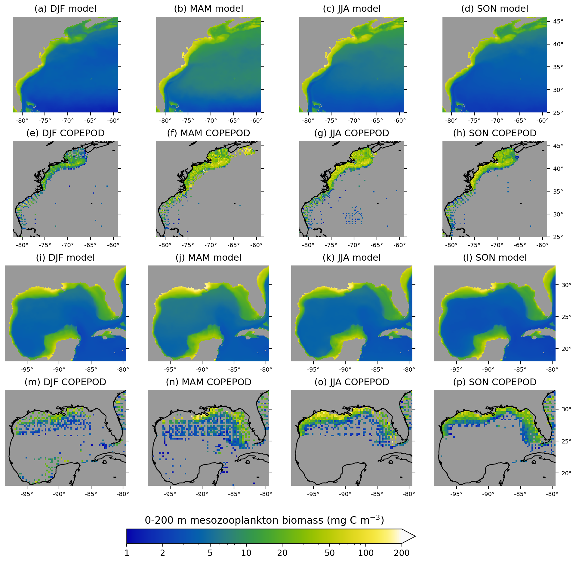
Figure 14The 0–200 m average mesozooplankton biomass climatology along the US East Coast (a–h) and in the Gulf of Mexico (i–p). Observations from the COPEPOD dataset have been adjusted for approximate undersampling by scaling by a factor of 2.
Moving to the carbon system dynamics, the model annual average surface pCO2 is a close match to the SOCAT and data-derived products (Fig. 15a–f). The main bias relative to both observation-based products is higher modeled pCO2 in the subtropical gyre, a bias on the order of 10 %. The model also appears to have biases in the Gulf of St Lawrence and off the coast of Newfoundland and Labrador; however, the observation-based products contain fewer observations in this region and may be affected by seasonal ice cover (Landschützer et al., 2020a). Comparing the seasonal variability in pCO2 in the model with the machine-learning-based estimate of Landschützer et al. (2020a) (Fig. 15g–i), the model has higher variability along the coast and south of the Gulf Stream path and lower variability in the southern Labrador Sea in the northeast corner of the model domain. The bias toward a higher seasonal cycle amplitude was also found in a 0.5∘ global simulation with COBALT by Roobaert et al. (2022) and is likely attributable to the underestimation of the seasonality of non-thermal processes (i.e., biological update) in spring–summer and winter DIC mixing/supply in autumn–winter.
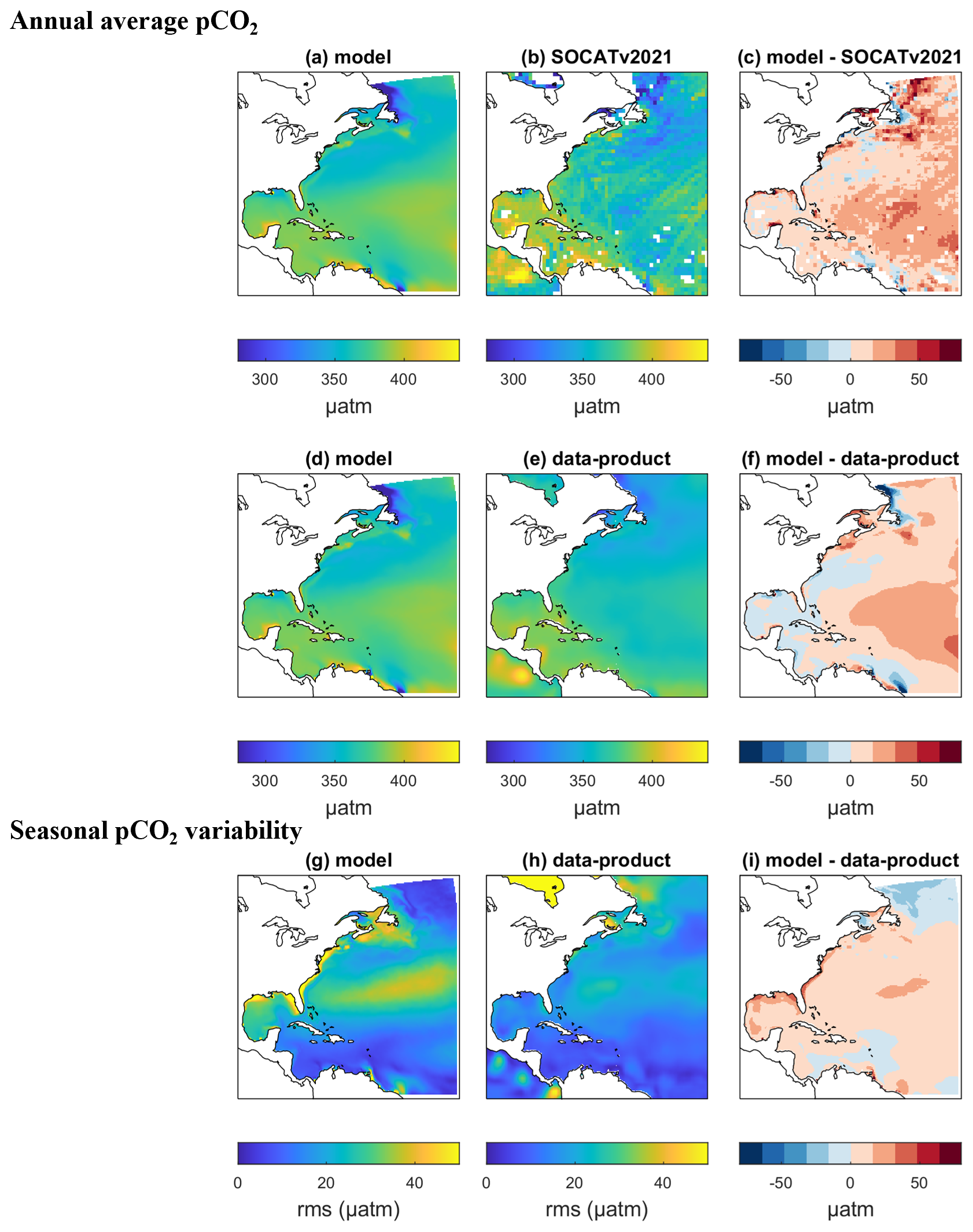
Figure 15Modeled (left) and observed (center) surface pCO2 spatial distributions (in µatm) and model bias (right) on annual average (a–f) and seasonal (g–i) timescales. The seasonal timescale evaluation is performed on the seasonal amplitude, which is expressed as the root mean square of the monthly climatology pCO2 anomalies (rms, in µatm). The model evaluation is performed directly against pCO2 observations derived from the Surface Ocean CO2 Atlas database version 2021 (SOCATv2021; Bakker et al., 2016) and against a pCO2 data product generated from the SOCAT observation by a two-step neural network interpolation (data product; Landschützer et al., 2020a).
Annual mean patterns in simulated alkalinity and dissolved inorganic carbon (DIC) generally agree with observation-based climatologies, with spatial correlations of 0.93 and 0.87, respectively, and mean biases that are minor compared to the range of values found across the domain (Fig. 16a–f). The primary alkalinity bias is a positive bias in the northeast United States and Canada, which is consistent with overly prominent high-alkalinity/high-DIC Gulf Stream waters. A low-alkalinity bias is evident in the southern parts of the model domain, particularly in the vicinity of large freshwater outputs in Central and South America. This region is associated with a freshwater bias (Fig. 4), suggesting that the bias may arise from overly prominent low-alkalinity freshwater fluxes in this region. However, the observations in this region are highly uncertain: the GLODAPv2 dataset, which the Jiang et al. (2022) product sources are from, contains almost no observations in the Caribbean and Gulf of Mexico (Lauvset et al., 2021). The model DIC biases have a similar spatial pattern to the alkalinity biases, which is consistent with these properties being driven by the same processes, although the magnitude of the DIC biases is lower.
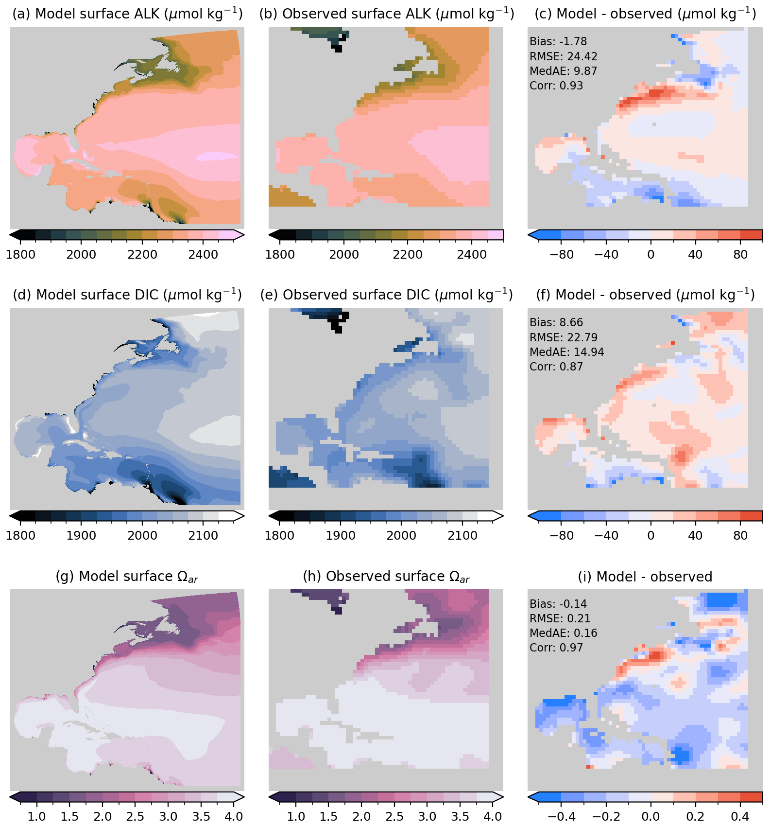
Figure 16Mean surface alkalinity (a–c), dissolved inorganic carbon (d–f), and aragonite saturation state (g–i) in the model (a, d, g) and the observation-derived climatology (b, e, h) and showing the difference between the model and observations (c, f, i).
The modeled and observed surface aragonite saturation exhibits a similar negative gradient with latitude (Fig. 16g–i), and the model is highly correlated with the observations (r=0.97). While none of the mean values at the surface fall below a saturation state and only a few grid cells in nearshore estuarine areas fall below the value of 1.5 that is considered suboptimal (Siedlecki et al., 2021), much of the northeastern coast of the United States and Canadian coastal waters falls below 2. In the high-alkalinity waters of the tropical North Atlantic, by contrast, the saturation state is often >4. The largest discrepancies in the model occur in the Mid-Atlantic Bight, which tends to have a greater component of high-Ωar tropical water and is consistent with the stronger Gulf Stream influence noted previously, and in the Gulf of Mexico, where the observations may not sample the nearshore region of a low-saturation state.
3.2 Relevant regional features and biogeochemical responses
As described in the Introduction, one of the challenges for the intended applications of the modeling system described herein is to connect large-scale ocean dynamics to regional responses. This requires the model to capture both the large-scale patterns (described in the preceding section) and more local marine resource relevant dynamics. One of the largest and most impactful changes in recent decades has been the substantial warming in the northwest Atlantic Ocean, particularly along the northeast US coast. The model is largely able to simulate the observed linear SST trends over 2005–2019, with an overall spatial correlation of 0.90–0.91 and negligible mean bias (Fig. 17). Both OISST and the GLORYS12 reanalysis show a broad pattern of surface cooling at the southern edge of the subpolar gyre in the northwestern corner of the domain and surface warming north of the Gulf Stream along the continental shelf and shelf break, which appears to be consistent with the predicted effect of a weakening Atlantic Meridional Overturning Circulation (Caesar et al., 2018), and this pattern is reproduced well in the model. However, there is some mismatch between the modeled and observed trends at fine scales along the shelf: the model temperature increase is too large along the Mid-Atlantic Bight and too small (although still positive) in the Gulf of Maine and Scotian Shelf and offshore of these regions beyond the shelf break.
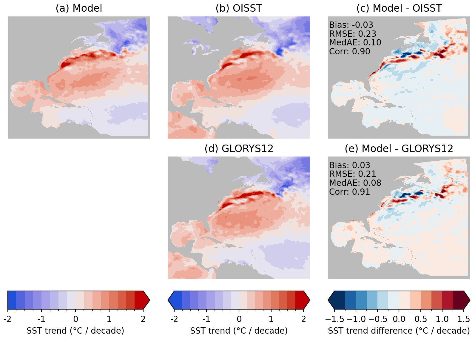
Figure 17The 2005–2019 sea surface temperature trends from the model (a) compared with trends from the OISST (b) and GLORYS12 (d) datasets and the difference between the model and the datasets (c, e).
The model reliably simulates most aspects of the seasonal variation in temperature and mixing in the four northeast US EPUs (Fig. 18). The most notable deficiency in the model stems from the warm surface temperature bias in winter and spring (seen in Fig. 3), which extends throughout the mixed layer of each EPU. This bias results in an absence of the cool intermediate layer centered at about 60 m typically seen in summer. Despite this bias, the depth of the winter and spring mixing is generally consistent with the reanalysis climatology, suggesting the surface heat forcing as a possible cause of the bias.
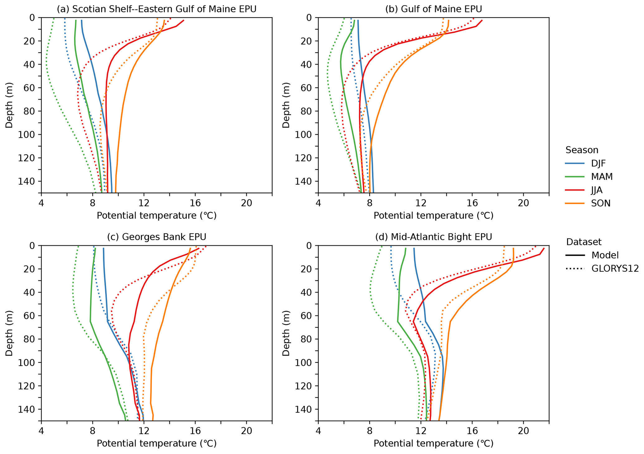
Figure 18Vertical profiles of seasonal temperature climatologies in four different northeast US ecological production units computed from model and reanalysis data.
The interannual bottom-temperature variability within the EPUs is simulated well by the model, although long-term trends are missed in some regions (Fig. 19). The correlation between the modeled and observed or reanalysis anomalies is highest in Georges Bank, where strong mixing couples the bottom-temperature variability with the atmospheric forcing, and the Mid-Atlantic Bight, and it is lowest in the Gulf of Maine. Observations and reanalysis data from all EPUs show a general pattern of a sharp cold snap in 2004 that was associated with deep winter mixing (Taylor and Mountain, 2009) followed by a strong warming trend. Although the model reproduces these trends and the superimposed variability to some extent, it substantially underestimates the warming trend in the EPUs covering the Gulf of Maine and southwestern Scotian Shelf. These underestimated bottom trends are consistent with the underestimated SST trends in these regions (Fig. 17). On the other hand, the observed and reanalysis time series began to diverge around 2010, with the reanalysis warming faster than the observations, and the model is generally closer to the observations than the reanalysis during this period.
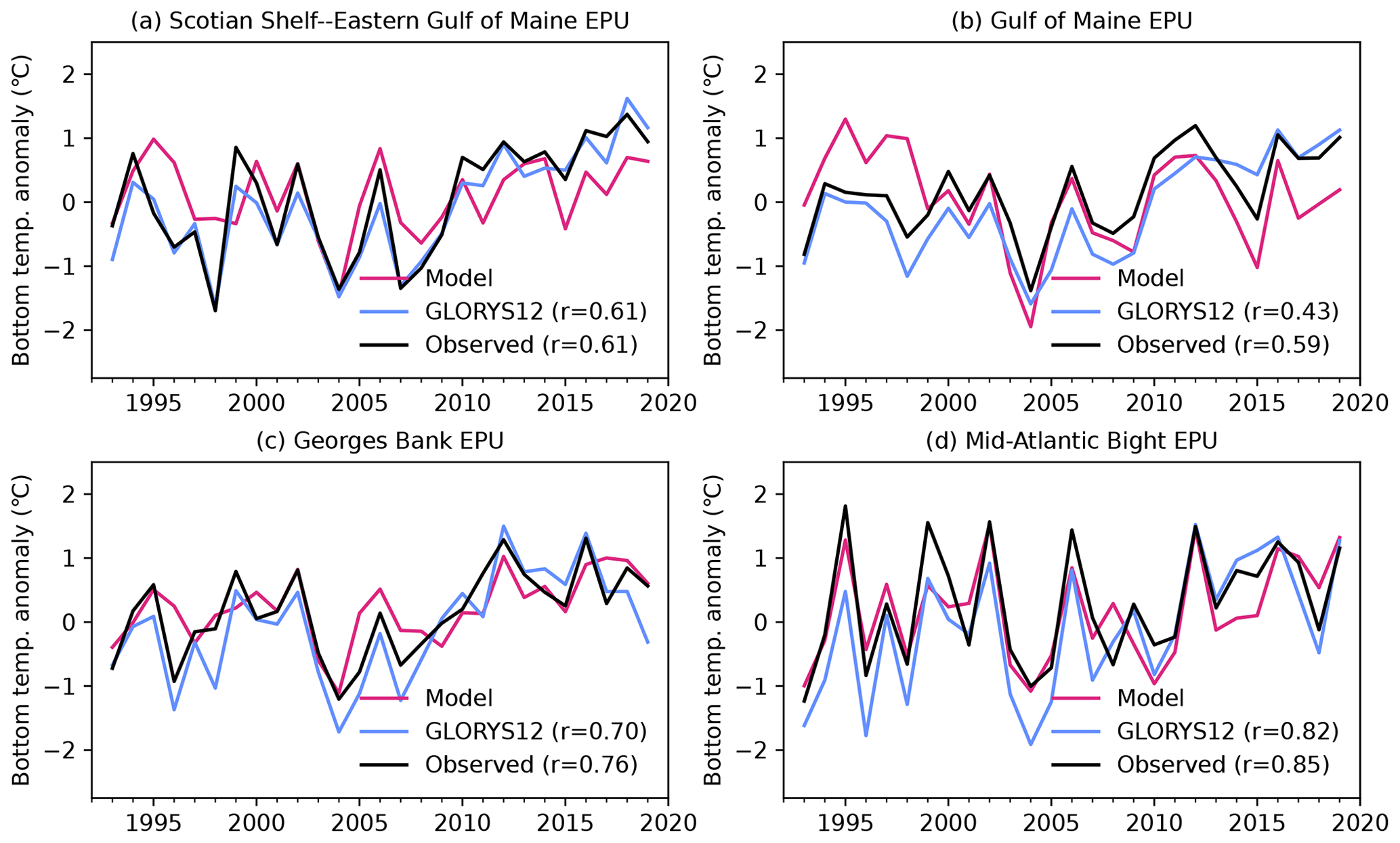
Figure 19Annual average bottom-temperature anomalies in four different northeast US ecological production units computed from model, reanalysis, and observed data.
The mean and range of modeled temperature and salinity at 150–200 m depth in the Gulf of Maine Northeast Channel are broadly consistent with the data from CTD and buoy observations and the GLORYS12 reanalysis (Fig. 20a). Relative to the reanalysis, the average model salinity is too high by 0.12 and the average model temperature is too warm by 0.25 ∘C. Compared to the analysis of Saba et al. (2016), this warm bias is less than the warm bias of the ∘ CM2.6 climate model and substantially less than the warm bias of several degrees found in the ∘ CM2.5 climate model, which highlights the benefits of high-resolution downscaling. Although the reanalysis, CTD, and moored-buoy data products all have slightly different means and ranges of temperature and salinity, all three products and the model show the same mixing of predominantly Warm Slope Water (WSW) and Labrador Slope Water (LSW) with a minor addition of Scotian Shelf Water. Compared to all three data products, however, the model temperature and salinity variability is confined within a smaller range. The model has relatively poor skill at simulating the time series of the mixing between these water masses (Fig. 20b–c); over the full 1993–2019 time period, the correlation between the model and data-derived water masses ranges from 0.30 to 0.43. Compared to the mooring-derived water masses, which are only available from 2004–2017, the model has much higher correlations of 0.82 for both LSW and WSW. This difference in correlation is due to the model missing several prominent fluctuations in water masses during the early part of the time series, including the significant drop in WSW in 1998, and accurately simulating many of the more recent fluctuations, including the second drop in WSW in 2007–2008 and the subsequent rebound. All three data products show this rebound and a continued increase in WSW persisting through 2019, although the products diverge from each other to some extent during this time. The model also simulates some increase in WSW and decrease in LSW after 2010, although the changes are less pronounced than in any of the data products.
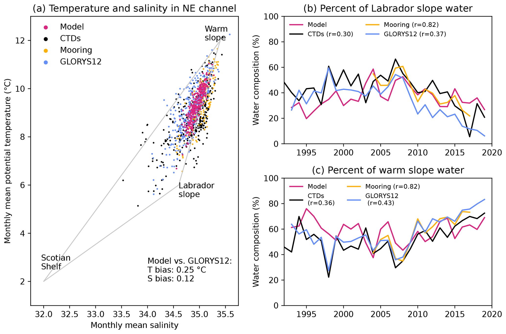
Figure 20(a) Monthly potential temperature and salinity between 150–200 m within the Northeast Channel compared with known water masses. (b–c) Time series of the composition of the water between 150–200 m within the Northeast Channel in terms of Labrador Slope Water (b) and Warm Slope Water (c). Each correlation in parentheses gives the correlation between the model time series and the given observation dataset.
Model bottom temperatures in the Mid-Atlantic Bight cold-pool region are biased warm by 0.70 ∘C on average (Fig. 21a–c), which is consistent with the warm bias seen in SST in this region. The model broadly simulates the spatial pattern of temperature associated with the cold pool with a spatial correlation coefficient between the model and GLORYS12 reanalysis of 0.88. Year-to-year variability in temperature anomalies associated with the cold pool, as indicated by the index of du Pontavice et al. (2022) based on June–September average bottom-temperature anomalies, also tracks the reanalysis data reasonably well (correlation coefficient between time series of 0.57) considering that this feature is typically challenging to model. This correlation is lower than the correlation of 0.85 between survey and model annual average bottom-temperature anomalies across the Mid-Atlantic Bight EPU (Fig. 19d), which is consistent with higher model skill during winter and spring when the water column is well mixed and bottom temperatures are connected to atmospheric forcing.
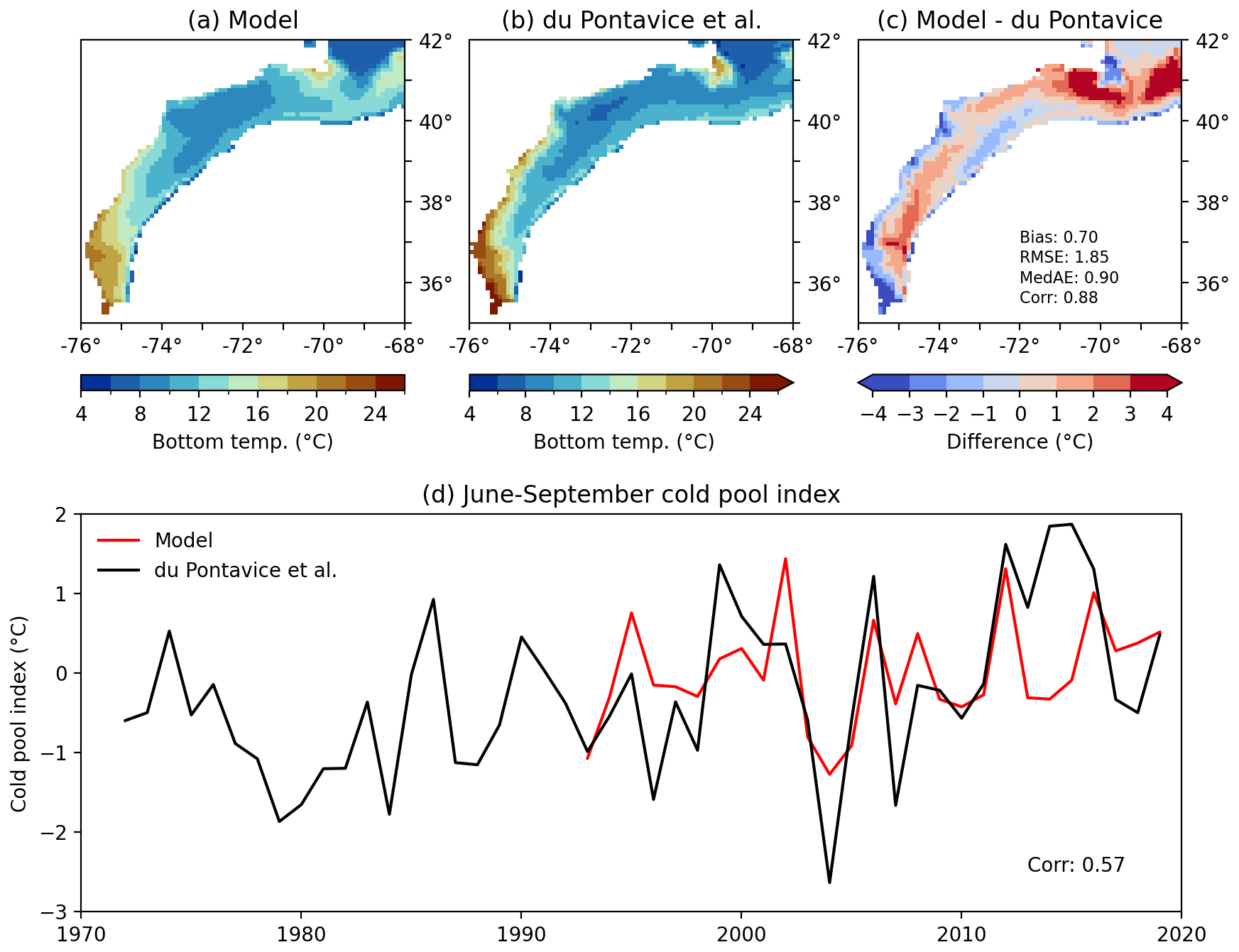
Figure 21Bottom temperature from the model (a) and du Pontavice et al. (2022) (b) in the cold-pool region averaged over June–September and the difference between the two datasets (c). (d) Comparison of the model cold-pool index, based on bottom-temperature anomalies, with the same index calculated from a regional ocean model (before 1993) and the GLORYS reanalysis (1993–2019) data by du Pontavice et al. (2022).
The model reliably simulates the spatial and temporal evolution of sea ice in the northwestern portion of the model domain (Figs. 22–23). The model has a modest bias toward earlier freezing and melting (Fig. 22), with more extensive sea ice coverage than observed in December and January and less in April. The low bias in April may be due to the omission of open boundary conditions for sea ice in the model, which does not allow the transportation of sea ice by the Labrador Current through the northern model boundary and into the domain (note that a low bias is also present near the boundary in January–March; Fig. 22f, i, l). The time series of monthly sea ice extent in the Gulf of St Lawrence (Fig. 23) shows that the model captures nearly all of the year-to-year variability in sea ice coverage in the gulf, with correlation coefficients between 0.94 in January and 0.96 in February. The satellite data show an abrupt shift toward lower and more variable ice coverage beginning around 1995, and this shift is correctly simulated by the model (although the model simulation only began in 1993, and thus it is not certain whether the model reproduces the relatively stable period before 1995).
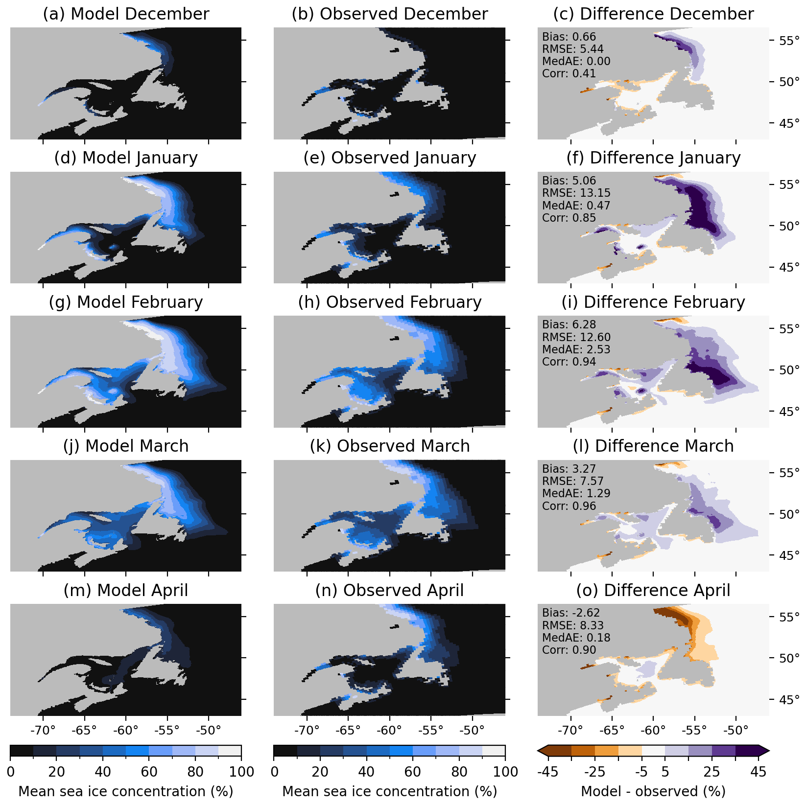
Figure 22The 1993–2019 monthly climatology of sea ice concentration from the model (left panels) and a satellite observation dataset (Cavalieri et al., 1996) (middle panels) and the difference between the two datasets (right panels).
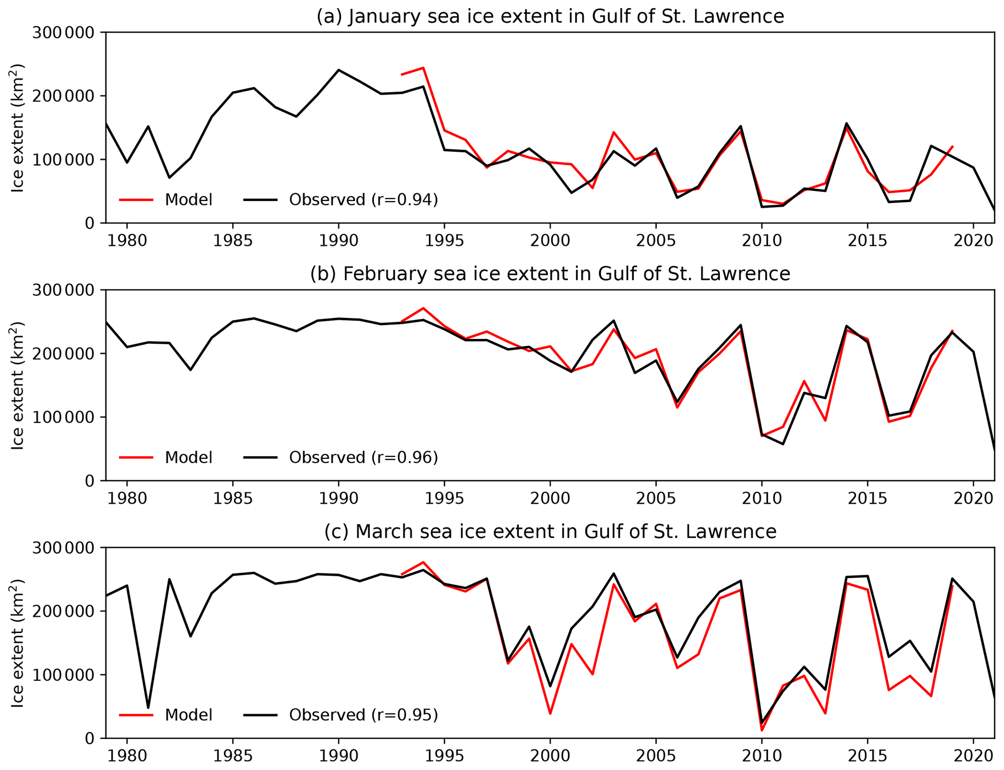
Figure 23Time series of the extent of sea ice within the Gulf of St Lawrence during January (a), February (b), and March (c) from the model and the satellite observation dataset (Cavalieri et al., 1996).
The model reproduces the primary response of surface chlorophyll in the Gulf of Mexico to both the El Niño and the La Niña phases of ENSO, although the magnitude of the model response is not as large (Fig. 24a–d). In the satellite observations, surface chlorophyll is higher than normal along the majority of the northern Gulf of Mexico coast during the winter and spring seasons of an El Niño event (Fig. 24a–d), although, as noted before, satellite estimates should be interpreted with caution in this turbid nearshore region. The model simulates a positive chlorophyll response offshore of the Mississippi River delta and the western Gulf of Mexico but fails to simulate the enhanced chlorophyll along the West Florida Shelf. In agreement with Gomez et al. (2019), the observed chlorophyll response during a La Niña winter and spring is opposite and slightly weaker compared to the response during El Niño (Fig. 24e–h). The model and remote sensing datasets generally agree that chlorophyll is lower than average over the majority of the region during La Niña winters. The model also reproduces increased surface chlorophyll near the mouth of the Mississippi River and decreased chlorophyll along the Louisiana–Texas Shelf during La Niña springs. However, the model again fails to simulate low-chlorophyll anomalies along the West Florida Shelf and southeast US coast. Across the region plotted in Fig. 24, the rank correlation between the model and satellite anomalies is slightly higher in spring than in winter for both El Niño and La Niña years.
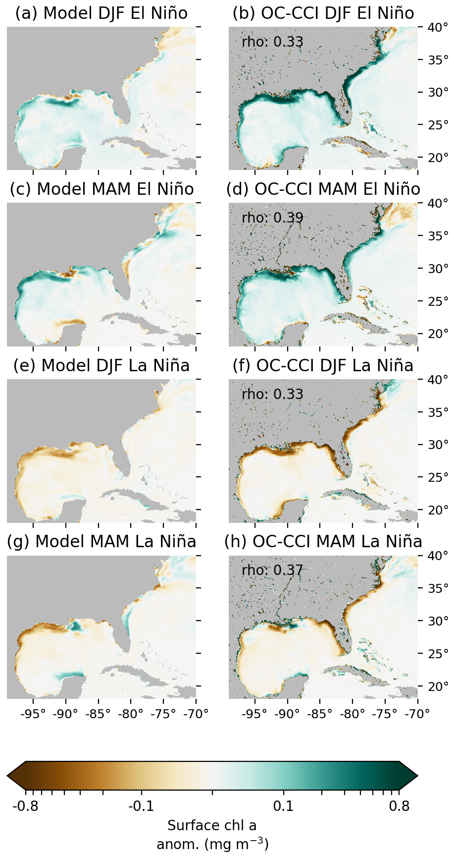
Figure 24Winter and spring surface chlorophyll a anomalies during El Niño years in the model (a, c) and satellite estimates (b, d), compared with the same during La Niña years (e–h). To display the wide range of chl a anomalies, values within ±0.1 mg m−3 are shaded on a linear scale, while values outside of this range are shaded on a logarithmic scale. Annotated correlation values give the Spearman rank correlation between the model and satellite anomalies over the plotted region.
Finally, bottom hypoxia along the Louisiana–Texas Shelf is simulated reasonably well by the model (Fig. 25), especially given the small scale over which this hypoxia occurs, the omission of extremely shallow areas in the model bathymetry (which has a minimum depth of 10 m), and the basic representation of coastal benthic processes in COBALT. The seasonal variation in the hypoxic area in the model, peaking in July, is consistent with the area estimated from cruise observations and other data by Matli et al. (2020) during the months of May–September (Fig. 25a). In all months, the model hypoxic area is less than the observed area. During July, the model underpredicts the hypoxic area by 3962 km2 on average, or about 25 % of the observed area (Fig. 25b). About of the interannual variability is correctly predicted by the model (r=0.51).
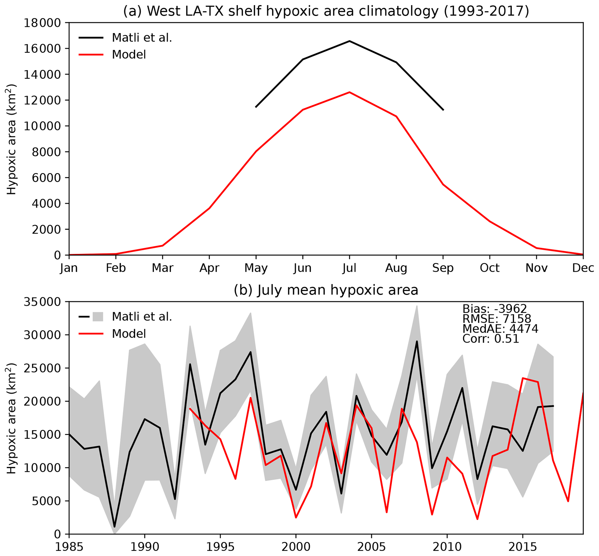
Figure 25Monthly climatologies of hypoxic area (area with a July mean bottom oxygen concentration below 2 mg L−1) over the LA–TX Shelf from the model and geostatistical estimates from Matli et al. (2020) (a) and time series of July mean hypoxic area from the model and Matli et al. (2020) (b). Gray shading in (b) denotes the 95 % confidence interval for the Matli et al. (2020) data.
3.3 Computational performance
In Fig. 26, we evaluate the total run time of the model with several choices of grid decomposition to determine whether the computational cost of the model is low enough to enable running the large ensembles of long simulations that are needed to support the intended applications. Using the 40 × 40 decomposition, which distributes the 775 × 845 model grid onto a 40 × 40 grid of processing elements (PEs), the model can run 1 year of simulation in about 9 h of wall clock time. As the number of PEs is increased, the wall clock time is reduced; however, due to parts of the model that are run in serial (e.g., we used a single process to write the model output, although the option exists to do this in parallel) and inefficiencies in parts that are run in parallel, the total computational cost increases with the number of PEs. The total cost of the 50 × 50 case is slightly less than 1.25 times the cost of the 40 × 40 case, and the cost of the 60 × 60 case is slightly more than 1.25 times the cost; both are reasonable trade-offs between run time and computational cost. The 70 × 70 case is less efficient, with a total cost of more than 1.5 times the cost of the 40 × 40 case. Despite the increased total computational costs of the larger PE layouts, these layouts support run times fast enough to meet our informal performance criterion of 3 simulation years per day. All layouts except the 40 × 40 case exceed this threshold, which allows them to run nearly a century of continuous simulation in 1 month (assuming no cluster queue wait time). Furthermore, the scaling efficiency of this tracer-heavy model is better than seen in MOM6 models without coupled biogeochemistry where the computationally expensive 2-dimensional barotropic solver generally ceases to scale with fewer than 15 × 15 points per PE. The 40 additional tracers added by the BGC component result in more time spent in the tracer routines, which scale fairly well as the number of points per PE is reduced (and total PEs are increased), and produce a meaningful reduction in run time even though the time spent in the barotropic solver remains roughly constant.
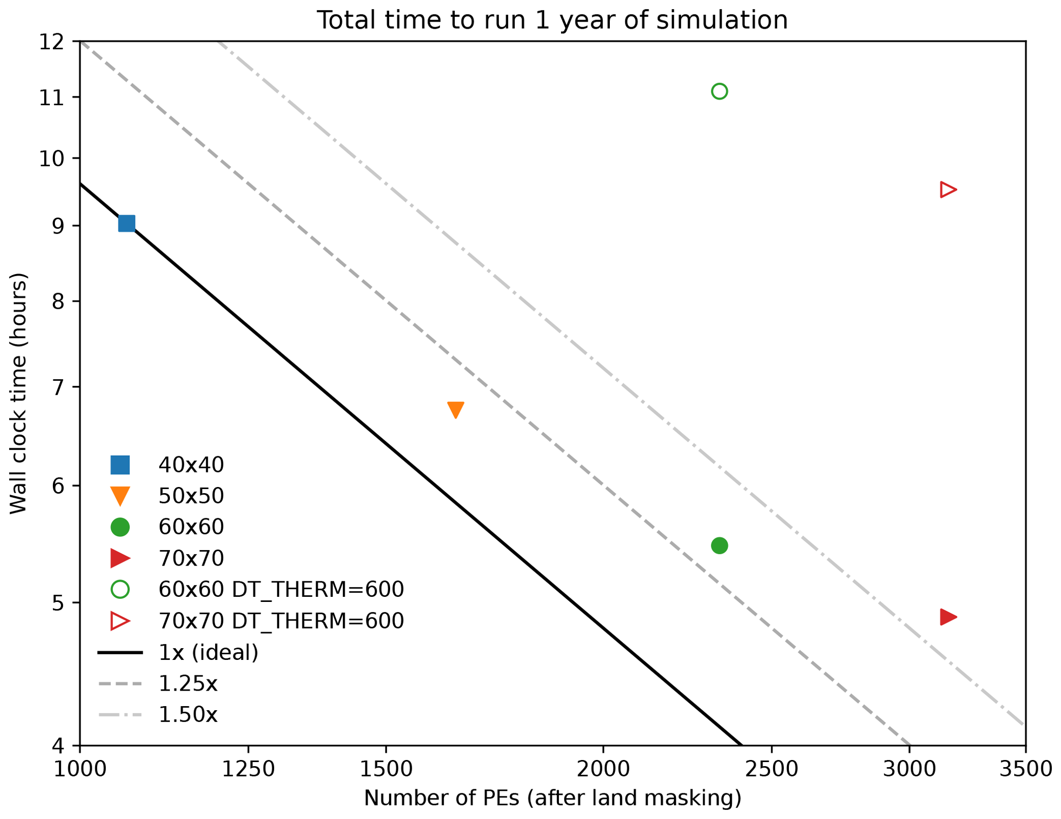
Figure 26Total wall clock time needed to run 1 year of model simulation as a function of the number of processing elements (PEs). Shapes and colors indicate the grid of PEs onto which the model domain is distributed before eliminating all-land PEs. Diagonal lines are lines of constant computational cost (processes × time) relative to the 40 × 40 case. The two empty shapes are simulations with the thermodynamics time step set to the same as the dynamics time step. Both plot axes are on a logarithmic scale.
A key feature of MOM6 that improves the computational economy is the ability to efficiently integrate the thermodynamics and tracer processes over a longer time step than the baroclinic and barotropic dynamics time steps that are highly limited by stability concerns. Because the coupled COBALT biogeochemical model integration is called during the thermodynamics time step and COBALT introduces 40 new tracers that must be advected and diffused by the ocean model component during the thermodynamics time step, taking longer thermodynamics time steps can substantially reduce the total computational cost of the model. In the present configuration, we use an 1800 s thermodynamics time step, which is 3 times longer than the 600 s baroclinic time step. To evaluate the cost savings of this feature, we ran two experiments with a 600 s thermodynamics time step and plotted the run times as empty shapes in Fig. 26. For a given grid decomposition, an 1800 s thermodynamics time-step results in a decrease by a factor of 2 in the total run time compared to a 600 s thermodynamics step. MOM6 is also computationally efficient at handling tracers in general: using the 1800 s thermodynamics step, the inclusion of coupled COBALT biogeochemistry and its 40 tracers only results in an increase about 2.5 times the computational cost (not shown).
MOM6-COBALT-NWA12 exhibited good performance in simulating a wide range of ecosystem-relevant physical and biogeochemical diagnostics while also satisfying computational performance constraints. Long-term means and seasonal climatologies were simulated well for nearly all metrics, with the main biases across quantities often related to challenges in simulating the Gulf Stream. The ∘ resolution used here is only slightly higher than the ∘ resolution considered to be a necessary but not sufficient condition for resolving the Gulf Stream separation and path (Chassignet and Marshall, 2008). A version of the model with a highly refined resolution, on the order of ∘ or ∘, may improve the Gulf Stream path and variability and reduce the biases, as has been found in studies of other models on similar domains (Chassignet and Xu, 2017, 2021). However, such increases in resolution would also greatly increase the computational costs. An 8-fold increase in computational cost is generally incurred for each doubling of the horizontal grid resolution (4 times for the increase in the number of grid cells and 2 times for the required time step decreases to maintain numerical stability, although in MOM6 the thermodynamics time step need not be decreased with increasing resolution and this factor may be more favorable). We are currently running higher-resolution simulations to better quantify the model skill and computational cost trade-offs associated with enhanced resolution in the NWA12 domain.
Metrics that evaluate the model on the basis of interannual to decadal variability, rather than long-term means, also showed significant skill, particularly for lower-frequency variations, along with some errors possibly related to the Gulf Stream bias. Variability in the Gulf Stream position, bottom temperatures in the northeast US EPUs, sea ice in the Gulf of St Lawrence, and sea surface temperature trends all compared reasonably well with the respective observed time series. However, the model slightly underestimated recent surface warming in the Gulf of Maine and largely failed to simulate the recent bottom warming, and the composition of deep water in the Northeast Channel was only moderately coherent with observations during the full 1993–2019 time period, though agreement with buoy data over the last 15 years was stronger. Some of the lower performance in this region may be caused by unpredictable stochastic variability, such as warm-core eddies shed from the Gulf Stream that bring warm and salty water to the shelf and coast (Du et al., 2021; Gawarkiewicz et al., 2019) and eddies propagating from the tail of the Grand Banks (Brickman et al., 2018). While eddies are present at ∘ resolution, the formation and evolution of individual eddies are not deterministically simulated without data assimilation. This is consistent with the lower correlation with observations for the monthly Gulf Stream index compared to the 25-month rolling mean.
During development of the model, we found several parameters that exerted a strong influence over the physical properties of the model simulation. First, the separation point and path of the Gulf Stream were influenced by the biharmonic viscosity parameters: higher viscosity produced a later, northerly separation, and lower viscosity produced an earlier, southerly separation. This result is consistent with numerous other studies using other models (e.g., Bryan et al., 2007; Chassignet and Garaffo, 2001). Our biharmonic viscosity parameterization, the maximum of a velocity scale of 1 cm s−1 times the grid spacing cubed and a Smagorinsky viscosity with a coefficient of 0.015, results in a typical viscosity of about 3.8×10⁹ m4 s−1 at the latitude of Cape Hatteras. The viscosity cannot be substantially reduced at this resolution without introducing grid-scale noise and instabilities or increased without shifting the Gulf Stream separation northward and exacerbating the warm-temperature biases along the shelf. Compared to other studies, the viscosity in the MOM6-COBALT-NWA12 is lower than the viscosity in the 0.1∘ ocean resolution models of Li et al. (2022) and Sasaki et al. (2020). The velocity scale of 1 cm s−1 is the same as the ∘ and ∘ models of Adcroft et al. (2019), although A19 used a higher Smagorinsky coefficient of 0.06 and included an additional Laplacian viscosity in regions of the ∘ model where the resolution was coarser than the first baroclinic deformation radius. Chassignet and Garaffo (2001) and Chassignet and Xu (2017) also used the same biharmonic velocity scale; however, Chassignet and Garaffo (2001) found that a small biharmonic viscosity alone produced an early separation of the Gulf Stream and could only obtain an accurate simulation with Laplacian viscosity added everywhere in the model domain. Aside from viscosity, MOM6-COBALT-NWA12 has other differences from these models, including explicit tides and z∗ vertical coordinates rather than isopycnal or hybrid coordinates, and identifying which factors contribute to obtaining a satisfactory simulation with lower viscosity is left for future work. This line of research is likely to benefit from the flexible vertical coordinate capability of MOM6.
Second, the front length specified in the parameterization for restratification by submesoscale eddies has a strong control over the mixed-layer depth in MOM6, as noted by Adcroft et al. (2019). The front length of 1500 m used here is greater than the 500 m used in Adcroft et al. (2019), which results in a decreased restratification effect. The front length is also greater than suggested by the scaling developed by Bodner et al. (2023), which predicts front lengths shorter than even 500 m throughout most of the NWA12 model domain. Shorter front lengths would decrease mixed-layer depths, which would be beneficial in some regions of the domain that have a bias toward deeper winter mixed layers (Fig. 5). However, the reduced mixing caused by a stronger restratification effect would have other impacts, including increasing the bottom-temperature bias and reducing the extent of the cold pool in the Mid-Atlantic Bight (Fig. 21). The chosen value of 1500 m is thus a reasonable compromise.
Finally, the coefficient used in the scalar approximation of the effect of tidal self-attraction and loading (SAL) has a strong control on tidal range in the model, particularly in the Gulf of Maine and Gulf of St Lawrence. In this scalar SAL approximation, the effect of SAL is equal to a single, constant coefficient times the local model free-surface elevation. The coefficient value of 0.01 used in this study is significantly lower than values ranging from 0.085–0.12 commonly used in global tide models (Accad and Pekeris, 1978; Ray, 1998; Stepanov and Hughes, 2004). In the NWA12 regional model, increasing the SAL coefficient increases M2 amplitude in the Gulf of St Lawrence and decreases it in the southwest Gulf of Maine. Increasing SAL above 0.01 would thus reduce the Gulf of Maine M2 amplitude bias in the current model but increase it in the Gulf of St Lawrence (Fig. 8). The value of 0.01 is a compromise between these two biases and the effects they have on regional hydrodynamics. In reality the effect of SAL is not constant but varies as a function of the tidal spatial scales (which in turn vary with water depth) and other factors (Ray, 1998; Stepanov and Hughes, 2004), and modeling studies have found that the coefficient should be smaller than the typical 0.085–0.12 over most of the Atlantic Ocean and particularly in the Gulf of Mexico and along the US East Coast (Irazoqui Apecechea et al., 2017; Stepanov and Hughes, 2004). We consider the scalar value of 0.01 to produce results that are sufficiently accurate for the intended use of the current version of the model, but separate ongoing studies may explore the effect of more sophisticated models of SAL and the impacts on coastal hydrodynamics.
As a first step toward the goal of providing information about historical ocean-ecosystem conditions and possible future changes that could support living-marine-resource management and applications, we developed a regional model of ocean dynamics and biogeochemistry for the northwest Atlantic Ocean. Comparison of a model historical simulation with data from reanalysis and observations showed that the model generally performed well at simulating both historical mean conditions and significant trends and variability with minimal drift. This suggests that the model can provide the accurate information needed for many applications; notably, several of the evaluation metrics in this paper and the observations for them were taken directly from reports used to inform fishery managers. However, more detailed skill evaluations specific to each intended application will likely be necessary to better understand the reliability of and uncertainty in the model simulations.
Not all aspects of the model simulation reproduced the observations as well as might be desired. Interannual variability of fine-scale features, including the Mid-Atlantic Bight cold pool and the area of hypoxia along the LA–TX Shelf, were simulated with correlation coefficients around 0.5, which is often considered a lower bound for useful prediction skill (Murphy and Epstein, 1989). Recent warming at the surface and bottom of the Gulf of Maine was also underestimated. Future model simulations focused more specifically on these regions may benefit from employing additional downscaling by nesting a ∘ or higher local model within the ∘ regional NWA12 domain to obtain some of the benefits of higher resolution with a lower computational cost. Adjustments to the spacing of the vertical coordinates to enhance resolution in coastal areas or switching from the z level to an adaptive hybrid coordinate that is locally terrain following may also improve the simulation of these features. Nested local domains would also allow adjusting the model parameters, such as the mixed-layer eddy front length and tidal self-attraction and loading coefficient, to optimal values for each region. Furthermore, as it was not possible in this paper to compare the model with every relevant metric and dataset within the entire NWA12 domain, development of local domains could focus on a more comprehensive evaluation for the local area. However, unless two-way nesting was employed, these smaller, nested domains would limit the applicability for large-scale issues like cross-boundary shifts in species distributions that may occur under climate change, and a proliferation of different models could introduce confusion and complexity and complicate development of the core model components.
Although historical model simulations can provide useful information for LMR applications, for example by reconstructing historical conditions when observations were sparse (du Pontavice et al., 2022), forecasts and projections of future conditions are essential for managing and adapting to the impacts of climate variability and change on LMRs (Tommasi et al., 2017b). Interdisciplinary research has repeatedly emphasized that forecast users benefit from being provided with information about forecast accuracy and uncertainty (e.g., Ramos et al., 2013; Roulston et al., 2006). However, providing reliable uncertainty information generally requires running long ensemble simulations, and the imposing computational costs of these simulations have limited the number of cases where this information is provided (Lewis et al., 2022). The model developed here takes advantage of the efficiency of MOM6 to achieve run times of more than 3 simulation years per day, our informal goal for a useful model that can run large ensembles in reasonable times. Although there are areas where this first version of the model can be improved, we believe it forms a useful starting point for following the recommendations of Dietze et al. (2018) by iteratively creating testable predictions that can both inform LMR applications and produce insights into how to improve the model and make better predictions.
Table A1Parameter values used for the four-phytoplankton-group COBALT formulation enlisted herein. The rationale underlying the variation in parameters across sizes and functional types is consistent with Stock et al. (2020), and further discussion can be found therein.
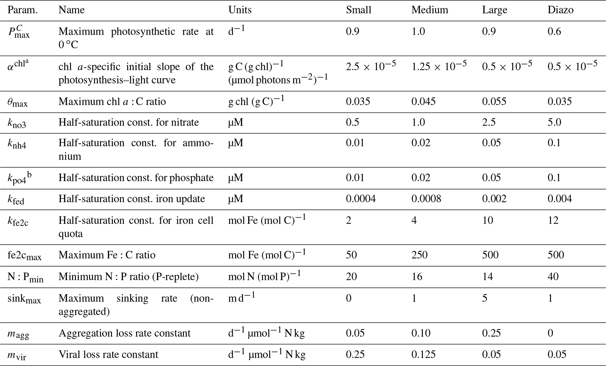
Table A2The innate prey availability applied for each zooplankton consumer (column) to each potential prey item (column). The maximum innate availability is 1. Prey switching between herbivory and carnivory is parameterized as described in Stock et al. (2008).
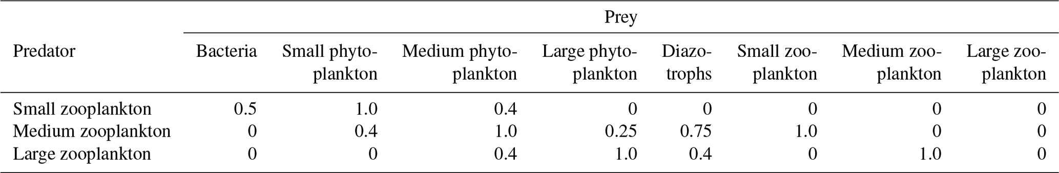
The source code for each component of the model has been archived at https://doi.org/10.5281/zenodo.7893349 (Ross et al., 2023b). MOM6 is built on an open development paradigm, and the Git repositories at https://github.com/mom-ocean/MOM6 (last access: 23 November 2023) and https://github.com/NOAA-GFDL/MOM6 (last access: 23 November 2023) provide a means for the community to obtain updated and experimental source code, report bugs, and contribute new features. Repositories for the other model components are also available at https://github.com/NOAA-GFDL (last access: 23 November 2023).
All model output that was analyzed in this paper has been published at https://doi.org/10.5281/zenodo.7893387 (Ross et al., 2023a). Model parameter files and prepared forcing files are published at https://doi.org/10.5281/zenodo.7893727 (Ross et al., 2023c).
The datasets used for comparison with the model and the URL or DOI where the data can be downloaded are listed as follows: GLORYS12 reanalysis (https://doi.org/10.48670/moi-00021, Global Ocean Physics Reanalysis, 2021); OISST v2 (https://psl.noaa.gov/data/gridded/data.noaa.oisst.v2.highres.html, Reynolds et al., 2007); regional temperature and salinity climatologies (https://www.ncei.noaa.gov/products/regional-ocean-climatologies, Seidov et al., 2018); mixed-layer depth (https://doi.org/10.17882/91774, de Boyer Montégut, 2023); global ocean gridded sea surface heights (https://doi.org/10.48670/moi-00148, Global Ocean Gridded L4 Sea Surface Heights And Derived Variables Reprocessed 1993 Ongoing, 2023); TPXO9 (https://www.tpxo.net/home, Egbert and Erofeeva, 2002); OC-CCI v6.0 (https://www.oceancolour.org/, Sathyendranath et al., 2019); COPEPOD (https://www.st.nmfs.noaa.gov/copepod/biomass/biomass-fields.html, Moriarty and O'Brien, 2013); World Ocean Atlas 2018 (https://www.ncei.noaa.gov/archive/accession/NCEI-WOA18, Boyer et al., 2019); SOCATv2021 (https://doi.org/10.25921/yg69-jd96, Bakker et al., 2021); surface pCO2 climatology (https://doi.org/10.25921/qb25-f418, Landschützer et al., 2020b); alkalinity, DIC, and aragonite saturation (https://doi.org/10.25921/g8pb-zy76, Jiang et al., 2022); EPU bottom temperatures (https://github.com/NOAA-EDAB/ecodata/releases/tag/3.0, Bastille, 2023); northeast US CTD profiles (ftp://ftp.nefsc.noaa.gov/pub/hydro/matlab_files/yearly, last access: 14 February 2021); Buoy N01 (http://www.neracoos.org/erddap/info/index.html?, NERACOOS, 2021); sea ice concentration (https://doi.org/10.5067/MPYG15WAA4WX, DiGirolamo et al., 2022); and cold-pool index (https://github.com/NOAA-EDAB/ecodata/releases/tag/3.0, Bastille, 2023).
The datasets used to create the model forcing and the URL or DOI where the data can be downloaded are listed as follows: GLORYS12 reanalysis (https://doi.org/10.48670/moi-00021, Global Ocean Physics Reanalysis, 2021), TPXO9 (https://www.tpxo.net/home, Egbert and Erofeeva, 2002), World Ocean Atlas (https://www.ncei.noaa.gov/archive/accession/NCEI-WOA18), GloFAS (https://doi.org/10.24381/cds.a4fdd6b9, Zsoter, 2021), USGS Gauge 07374525 (https://waterdata.usgs.gov/monitoring-location/07374525/), ERA5 (https://doi.org/10.24381/cds.adbb2d47, Hersbach et al., 2023), Carter et al. (2021) alkalinity and DIC estimation algorithm (https://doi.org/10.5281/zenodo.5512697), RC4USCoast (https://doi.org/10.25921/9jfw-ph50, Gomez et al., 2022), and GlobalNEWS2 (https://doi.org/10.1016/j.envsoft.2010.01.007, Mayorga et al., 2010); Meinshausen et al. (2017) atmospheric CO2 (https://doi.org/10.22033/ESGF/input4MIPs.1118, Meinshausen and Vogel, 2016; https://doi.org/10.22033/ESGF/input4MIPs.9866, Meinshausen and Nicholls, 2018). Data from Lavoie et al. (2021) and Stock et al. (2014) can be obtained by contacting the corresponding authors.
ACR, CAS, AA, RH, MJH, KH, NZ, RD, and WC contributed source code for regional MOM6, COBALT, SIS2, and/or other components of the model framework. ACR, CAS, EJD, FG, DK, DL, and JS contributed to preparation of model input files. ACR, CAS, EC, MA, HdP, FG, JGJ, DL, LR, AR, VS, and SS contributed to evaluation and interpretation of the model results. ACR and CAS prepared the initial draft of the manuscript. All coauthors participated in discussions during various stages of the model development and evaluation and read and approved the final version of the manuscript.
The contact author has declared that none of the authors has any competing interests.
Publisher's note: Copernicus Publications remains neutral with regard to jurisdictional claims made in the text, published maps, institutional affiliations, or any other geographical representation in this paper. While Copernicus Publications makes every effort to include appropriate place names, the final responsibility lies with the authors.
Vimal Koul and John Krasting are acknowledged for their helpful comments and suggestions on an internal review of the manuscript, and the two anonymous reviewers are thanked for their reviews that improved the manuscript. Advice from Mitch Bushuk on the remotely sensed sea ice data and suggestions from Sang-Ki Lee are also greatly appreciated. Andrew C. Ross, Enrique Curchitser, Dujuan Kang, James Simkins, Laure Resplandy, Sang-Ik Shin, and Samantha Siedleck were partly funded by grants from NOAA's Climate Program Office. Enrique Curchitser, Katherine Hedstrom, James Simkins, Fabian Gomez, and Wenhao Chen were partly funded by NOAA's climate portfolio. Enrique Curchitser, Katherine Hedstrom, James Simkins, and Dujuan Kang were partly funded by a grant from the Cooperative Institute for Modeling the Earth System. This study has been conducted using EU Copernicus Marine Service information: https://doi.org/10.48670/moi-00021, https://doi.org/10.48670/moi-00148.
This paper was edited by Andrew Yool and reviewed by two anonymous referees.
Accad, Y. and Pekeris, C. L.: Solution of the Tidal Equations for the M2 and S2 Tides in the World Oceans from a Knowledge of the Tidal Potential Alone, Philos. T. Roy. Soc. Lond. A-Math., 290, 235–266, https://doi.org/10.1098/rsta.1978.0083, 1978. a, b
Adcroft, A. and Campin, J.-M.: Rescaled Height Coordinates for Accurate Representation of Free-Surface Flows in Ocean Circulation Models, Ocean Model., 7, 269–284, https://doi.org/10.1016/j.ocemod.2003.09.003, 2004. a
Adcroft, A., Anderson, W., Balaji, V., Blanton, C., Bushuk, M., Dufour, C. O., Dunne, J. P., Griffies, S. M., Hallberg, R. W., Harrison, M. J., Held, I., Jansen, M. F., John, J., Krasting, J. P., Langenhorst, A., Legg, S., Liang, Z., McHugh, C., Radhakrishnan, A., Reichl, B. G., Rosati, T., Samuels, B. L., Shao, A., Stouffer, R., Winton, M., Wittenberg, A. T., Xiang, B., Zadeh, N., and Zhang, R.: The GFDL Global Ocean and Sea Ice Model OM4.0: Model Description and Simulation Features, J. Adv. Model. Earth Sy., 11, 3167–3211, https://doi.org/10.1029/2019MS001726, 2019. a, b, c, d, e, f, g
Alexander, M. and Scott, J.: The Influence of ENSO on Air-Sea Interaction in the Atlantic, Geophys. Res. Lett., 29, 46–1–46–4, https://doi.org/10.1029/2001GL014347, 2002. a
Alexander, M. A., Shin, S.-i., Scott, J. D., Curchitser, E., and Stock, C.: The Response of the Northwest Atlantic Ocean to Climate Change, J. Climate, 33, 405–428, https://doi.org/10.1175/JCLI-D-19-0117.1, 2020. a
Alfieri, L., Lorini, V., Hirpa, F. A., Harrigan, S., Zsoter, E., Prudhomme, C., and Salamon, P.: A Global Streamflow Reanalysis for 1980–2018, J. Hydrol., 6, 100049, https://doi.org/10.1016/j.hydroa.2019.100049, 2020. a
Amaya, D. J., Alexander, M. A., Scott, J. D., and Jacox, M. G.: An evaluation of high-resolution ocean reanalyses in the California current system, Prog. Oceanogr., 210, 102951, https://doi.org/10.1016/j.pocean.2022.102951, 2023. a
Andres, M.: On the Recent Destabilization of the Gulf Stream Path Downstream of Cape Hatteras, Geophys. Res. Lett., 43, 9836–9842, https://doi.org/10.1002/2016GL069966, 2016. a
Arakawa, A. and Lamb, V. R.: Computational Design of the Basic Dynamical Processes of the UCLA General Circulation Model, in: General Circulation Models of the Atmosphere, edited by: Chang, J., vol. 17, Methods in Computational Physics: Advances in Research and Applications, Elsevier, 173–265, https://doi.org/10.1016/B978-0-12-460817-7.50009-4, 1977. a
Baker, A. R. and Croot, P. L.: Atmospheric and Marine Controls on Aerosol Iron Solubility in Seawater, Mar. Chem., 120, 4–13, https://doi.org/10.1016/j.marchem.2008.09.003, 2010. a
Bakker, D. C. E., Pfeil, B., Landa, C. S., Metzl, N., O'Brien, K. M., Olsen, A., Smith, K., Cosca, C., Harasawa, S., Jones, S. D., Nakaoka, S., Nojiri, Y., Schuster, U., Steinhoff, T., Sweeney, C., Takahashi, T., Tilbrook, B., Wada, C., Wanninkhof, R., Alin, S. R., Balestrini, C. F., Barbero, L., Bates, N. R., Bianchi, A. A., Bonou, F., Boutin, J., Bozec, Y., Burger, E. F., Cai, W.-J., Castle, R. D., Chen, L., Chierici, M., Currie, K., Evans, W., Featherstone, C., Feely, R. A., Fransson, A., Goyet, C., Greenwood, N., Gregor, L., Hankin, S., Hardman-Mountford, N. J., Harlay, J., Hauck, J., Hoppema, M., Humphreys, M. P., Hunt, C. W., Huss, B., Ibánhez, J. S. P., Johannessen, T., Keeling, R., Kitidis, V., Körtzinger, A., Kozyr, A., Krasakopoulou, E., Kuwata, A., Landschützer, P., Lauvset, S. K., Lefèvre, N., Lo Monaco, C., Manke, A., Mathis, J. T., Merlivat, L., Millero, F. J., Monteiro, P. M. S., Munro, D. R., Murata, A., Newberger, T., Omar, A. M., Ono, T., Paterson, K., Pearce, D., Pierrot, D., Robbins, L. L., Saito, S., Salisbury, J., Schlitzer, R., Schneider, B., Schweitzer, R., Sieger, R., Skjelvan, I., Sullivan, K. F., Sutherland, S. C., Sutton, A. J., Tadokoro, K., Telszewski, M., Tuma, M., van Heuven, S. M. A. C., Vandemark, D., Ward, B., Watson, A. J., and Xu, S.: A multi-decade record of high-quality fCO2 data in version 3 of the Surface Ocean CO2 Atlas (SOCAT), Earth Syst. Sci. Data, 8, 383–413, https://doi.org/10.5194/essd-8-383-2016, 2016. a, b, c
Bakker, D. C. E., Alin, S. R., Castaño-Primo, R., Cronin, M., Gkritzalis, T., Kozyr, A., Lauvset, S. K., Metzl, N., Munro, D. R., Nakaoka, S., O'Brien, K. M., Olsen, A., Omar, A. M., Pfeil, B., Pierrot, D., Rodriguez, C., Steinhoff, T., Sutton, A. J., Tilbrook, B., Wanninkhof, R., Willstrand Wranne, A., Ahmed, M., Andersson, A., Apelthun, L. B., Bates, N., Battisti, R., Beaumont, L., Becker, M., Benoit-Cattin, A., Berghoff, C. F., Boutin, J., Burger, E. F., Burgers, T. M., Cantoni, C., Cattrijsse, A., Chierici, M., Cross, J. N., Coppola, L., Cosca, C. E., Currie, K. I., De Carlo, E. H., Else, B., Enright, M. P., Ericson, Y., Evans, W., Feely, R. A., Fiedler, B., Fransson, A., García-Ibáñez, M. I., Gehrung, M., Glockzin, M., González-Dávila, M., Gutekunst, S., Hermes, R., Humphreys, M. P., Hunt, C. W., Ibánhez, J., Severino P., Jones, S. D., Kitidis, V., Körtzinger, A., Kosugi, N., Landa, C. S., Landschützer, P., Lefèvre, N., Lo Monaco, C., Luchetta, A., Lutz, V. A., Macovei, V. A., Manke, A. B., Merlivat, L., Millero, F. J., Monacci, N. M., Negri, R. M., Newberger, T., Newton, J., Nickford, S. E., Nojiri, Y., Ohman, M., Ólafsdóttir, S. R., Sweeney, C., Ono, T., Palter, J. B., Papakyriakou, T., Peterson, W. T., Plueddemann, A. J., Qi, D., Rehder, G., Ritschel, M., Rutgersson, A., Sabine, C. L., Salisbury, J. E., Santana-Casiano, J. M., Schlitzer, R., Send, U., Skjelvan, I., Smith, K., Sparnocchia, S., Sullivan, K. F., Sutherland, S. C., Szuts, Z. B., Tadokoro, K., Tanhua, T., Telszewski, M., Theetaert, H., Vandemark, D., Voynova, Y. G., Wada, C., Weller, R. A., and Woosley, T. J.: Surface Ocean CO2 Atlas Database Version 2021 (SOCATv2021) (NCEI Accession 0235360), NOAA National Centers for Environmental Information [data set], https://doi.org/10.25921/yg69-jd96, 2021. a
Balch, W. M., Drapeau, D. T., Bowler, B. C., Record, N. R., Bates, N. R., Pinkham, S., Garley, R., and Mitchell, C.: Changing Hydrographic, Biogeochemical, and Acidification Properties in the Gulf of Maine as Measured by the Gulf of Maine North Atlantic Time Series, GNATS, Between 1998 and 2018, J. Geophys. Res.-Biogeo., 127, e2022JG006790, https://doi.org/10.1029/2022JG006790, 2022. a, b, c
Bastille, K.: Release 3.0. NOAA-EDAB/ecodata [dataset], https://github.com/NOAA-EDAB/ecodata/releases/tag/3.0, last access: 1 August 2023. a, b
Baumann, H., Jones, L., Murray, C., Siedlecki, S., Alexander, M., and Cross, E.: Impaired Hatching Exacerbates the High CO2 Sensitivity of Embryonic Sand Lance Ammodytes Dubius, Mar. Ecol. Prog. Ser., 687, 147–162, https://doi.org/10.3354/meps14010, 2022. a
Bell, R., Spring, A., Brady, R., Huang, A., Squire, D., Blackwood, Z., Sitter, M. C., and Chegini, T.: xarray-contrib/xskillscore: Metrics for verifying forecasts, Zenodo [code], https://doi.org/10.5281/zenodo.5173153, 2021. a
Bell, R. J., Richardson, D. E., Hare, J. A., Lynch, P. D., and Fratantoni, P. S.: Disentangling the Effects of Climate, Abundance, and Size on the Distribution of Marine Fish: An Example Based on Four Stocks from the Northeast US Shelf, ICES J. Marine Sci., 72, 1311–1322, https://doi.org/10.1093/icesjms/fsu217, 2015. a, b
Bennett, A. F. and Kloeden, P. E.: The Ill-Posedness of Open Ocean Models, J. Phys. Oceanogr., 11, 1027–1029, https://doi.org/10.1175/1520-0485(1981)011<1027:TIPOOO>2.0.CO;2, 1981. a
Bisagni, J. J. and Sano, M. H.: Satellite Observations of Sea Surface Temperature Variability on Southern Georges Bank, Cont. Shelf Res., 13, 1045–1064, https://doi.org/10.1016/0278-4343(93)90040-5, 1993. a
Bodner, A. S., Fox-Kemper, B., Johnson, L., Roekel, L. P. V., McWilliams, J. C., Sullivan, P. P., Hall, P. S., and Dong, J.: Modifying the Mixed Layer Eddy Parameterization to Include Frontogenesis Arrest by Boundary Layer Turbulence, J. Phys. Oceanogr., 53, 323–339, https://doi.org/10.1175/JPO-D-21-0297.1, 2023. a, b, c
Boivin-Rioux, A., Starr, M., Chassé, J., Scarratt, M., Perrie, W., Long, Z., and Lavoie, D.: Harmful Algae and Climate Change on the Canadian East Coast: Exploring Occurrence Predictions of Dinophysis Acuminata, D. Norvegica, and Pseudo-nitzschia Seriata, Harmful Algae, 112, 102183, https://doi.org/10.1016/j.hal.2022.102183, 2022. a
Boyer, T. P., Garcia, H. E., Locarnini, R. A., Zweng, M. M., Mishonov, A. V., Reagan, J. R., Weathers, K. A., Baranova, O. K., Seidov, D., and Smolyar, I. V.: World Ocean Atlas 2018, https://www.ncei.noaa.gov/archive/accession/NCEI-WOA18 (last access: 29 September 2020), 2019. a, b, c
Brickman, D., Hebert, D., and Wang, Z.: Mechanism for the Recent Ocean Warming Events on the Scotian Shelf of Eastern Canada, Cont. Shelf Res., 156, 11–22, https://doi.org/10.1016/j.csr.2018.01.001, 2018. a, b
Bryan, F. O., Hecht, M. W., and Smith, R. D.: Resolution Convergence and Sensitivity Studies with North Atlantic Circulation Models. Part I: The Western Boundary Current System, Ocean Model., 16, 141–159, https://doi.org/10.1016/j.ocemod.2006.08.005, 2007. a, b
Caesar, L., Rahmstorf, S., Robinson, A., Feulner, G., and Saba, V.: Observed Fingerprint of a Weakening Atlantic Ocean Overturning Circulation, Nature, 556, 191–196, https://doi.org/10.1038/s41586-018-0006-5, 2018. a, b
Cai, W.-J., Hu, X., Huang, W.-J., Murrell, M. C., Lehrter, J. C., Lohrenz, S. E., Chou, W.-C., Zhai, W., Hollibaugh, J. T., Wang, Y., Zhao, P., Guo, X., Gundersen, K., Dai, M., and Gong, G.-C.: Acidification of Subsurface Coastal Waters Enhanced by Eutrophication, Nat. Geosci., 4, 766–770, https://doi.org/10.1038/ngeo1297, 2011. a
Carolina Castillo-Trujillo, A., Kwon, Y.-O., Fratantoni, P., Chen, K., Seo, H., Alexander, M. A., and Saba, V. S.: An evaluation of eight global ocean reanalyses for the Northeast U.S. continental shelf, Prog. Oceanogr., 219, 103126, https://doi.org/10.1016/j.pocean.2023.103126, 2023. a, b
Carter, B. R., Bittig, H. C., Fassbender, A. J., Sharp, J. D., Takeshita, Y., Xu, Y.-Y., Álvarez, M., Wanninkhof, R., Feely, R. A., and Barbero, L.: New and Updated Global Empirical Seawater Property Estimation Routines, Limnol. Oceanogr. Meth., 19, 785–809, https://doi.org/10.1002/lom3.10461, 2021. a, b, c, d, e
Cavalieri, D. J., Parkinson, C. L., Gloersen, P., and Zwally, H. J.: Sea Ice Concentrations from Nimbus-7 SMMR and DMSP SSM/I-SSMIS Passive Microwave Data, Version 1, National Snow and Ice Data Center [data set], https://doi.org/10.5067/8GQ8LZQVL0VL, 1996. a, b, c, d
Chassignet, E. P. and Garaffo, Z. D.: Viscosity Parameterization and the Gulf Stream Separation, in: From stirring to mixing in a stratified ocean: Proceedings of the 12th `Aha Huliko'a Hawaiian Winter Workshop, University of Hawai'i at Mānoa, 37–41, https://www.coaps.fsu.edu/pub/eric/papers_html/Chassignet_Garraffo_01.pdf (last access: 23 November 2023), 2001 a, b, c
Chassignet, E. P. and Marshall, D. P.: Gulf Stream Separation in Numerical Ocean Models, in: Geophysical Monograph Series, edited by: Hecht, M. W. and Hasumi, H., American Geophysical Union, Washington, D. C., vol. 177, 39–61, ISBN 978-0-87590-442-9, https://doi.org/10.1029/177GM05, 2008. a, b
Chassignet, E. P. and Xu, X.: Impact of Horizontal Resolution (1/12∘ to 1/50∘) on Gulf Stream Separation, Penetration, and Variability, J. Phys. Oceanogr., 47, 1999–2021, https://doi.org/10.1175/JPO-D-17-0031.1, 2017. a, b, c
Chassignet, E. P. and Xu, X.: On the Importance of High-Resolution in Large-Scale Ocean Models, Adv. Atmos. Sci., 38, 1621–1634, https://doi.org/10.1007/s00376-021-0385-7, 2021. a, b, c
Chen, K. and Kwon, Y.-O.: Does Pacific Variability Influence the Northwest Atlantic Shelf Temperature?, J. Geophys. Res.-Oceans, 123, 4110–4131, https://doi.org/10.1029/2017JC013414, 2018. a
Chen, Z., Kwon, Y.-O., Chen, K., Fratantoni, P., Gawarkiewicz, G., Joyce, T. M., Miller, T. J., Nye, J. A., Saba, V. S., and Stock, B. C.: Seasonal Prediction of Bottom Temperature on the Northeast U.S. Continental Shelf, J. Geophys. Rese.-Oceans, 126, e2021JC017187, https://doi.org/10.1029/2021JC017187, 2021. a
Chi, L., Wolfe, C. L., and Hameed, S.: Intercomparison of the Gulf Stream in Ocean Reanalyses: 1993–2010, Ocean Model., 125, 1–21, https://doi.org/10.1016/j.ocemod.2018.02.008, 2018. a
Chi, L., Wolfe, C. L. P., and Hameed, S.: The Distinction Between the Gulf Stream and Its North Wall, Geophys. Res. Lett., 46, 8943–8951, https://doi.org/10.1029/2019GL083775, 2019. a
Claret, M., Galbraith, E. D., Palter, J. B., Bianchi, D., Fennel, K., Gilbert, D., and Dunne, J. P.: Rapid Coastal Deoxygenation Due to Ocean Circulation Shift in the Northwest Atlantic, Nat. Clim. Change, 8, 868–872, https://doi.org/10.1038/s41558-018-0263-1, 2018. a
Clark, S., Hubbard, K. A., Anderson, D. M., McGillicuddy, D. J., Ralston, D. K., and Townsend, D. W.: Pseudo-Nitzschia Bloom Dynamics in the Gulf of Maine: 2012–2016, Harmful Algae, 88, 101656, https://doi.org/10.1016/j.hal.2019.101656, 2019. a
Clark, S., Hubbard, K. A., Ralston, D. K., McGillicuddy, D. J., Stock, C., Alexander, M. A., and Curchitser, E.: Projected Effects of Climate Change on Pseudo-nitzschia Bloom Dynamics in the Gulf of Maine, J. Marine Syst., 230, 103737, https://doi.org/10.1016/j.jmarsys.2022.103737, 2022. a
Codiga, D. L.: Unified Tidal Analysis and Prediction Using the UTide Matlab Functions, Technical Report 2011-01, Graduate School of Oceanography, University of Rhode Island, Narragansett, RI, 59 pp., https://www.po.gso.uri.edu/~codiga/utide/2011Codiga-UTide-Report.pdf (last access: 23 November 2023), 2011. a
Dagg, M. J. and Breed, G. A.: Biological Effects of Mississippi River Nitrogen on the Northern Gulf of Mexico – a Review and Synthesis, J. Marine Syst., 43, 133–152, https://doi.org/10.1016/j.jmarsys.2003.09.002, 2003. a
de Baar, H. and de Jong, J.: Distributions, Sources and Sinks of Iron in Seawater, in: Biogeochemistry of Iron in Seawater, edited by: Turner, D. and Hunter, K. A., Wiley, New York, 123–253, ISBN 978-0-471-49068-5, 2001. a
de Boyer Montégut, C.: Mixed Layer Depth over the Global Ocean: An Examination of Profile Data and a Profile-Based Climatology, J. Geophys. Res., 109, C12003, https://doi.org/10.1029/2004JC002378, 2004. a, b, c, d
de Boyer Montégut, C.: Mixed layer depth climatology computed with a density threshold criterion of 0.03kg/m3 from 10 m depth value, SEANOE [dataset], https://doi.org/10.17882/91774, 2023. a, b
Dierssen, H. M.: Perspectives on Empirical Approaches for Ocean Color Remote Sensing of Chlorophyll in a Changing Climate, P. Natl. Acad. Sci. USA, 107, 17073–17078, https://doi.org/10.1073/pnas.0913800107, 2010. a
Dietze, M. C., Fox, A., Beck-Johnson, L. M., Betancourt, J. L., Hooten, M. B., Jarnevich, C. S., Keitt, T. H., Kenney, M. A., Laney, C. M., Larsen, L. G., Loescher, H. W., Lunch, C. K., Pijanowski, B. C., Randerson, J. T., Read, E. K., Tredennick, A. T., Vargas, R., Weathers, K. C., and White, E. P.: Iterative Near-Term Ecological Forecasting: Needs, Opportunities, and Challenges, P. Natl. Acad. Sci. USA, 115, 1424–1432, https://doi.org/10.1073/pnas.1710231115, 2018. a
DiGirolamo, N., Parkinson, C. L., Cavalieri, D. J., Gloersen, P., and Zwally, H. J.: Sea Ice Concentrations from Nimbus-7 SMMR and DMSP SSM/I-SSMIS Passive Microwave Data, Version 2, ASA National Snow and Ice Data Center Distributed Active Archive Center [data set], https://doi.org/10.5067/MPYG15WAA4WX, 2022. a
Dinnel, S. P. and Wiseman, W. J.: Fresh Water on the Louisiana and Texas Shelf, Cont. Shelf Res., 6, 765–784, https://doi.org/10.1016/0278-4343(86)90036-1, 1986. a
Donovan, M. K., Burkepile, D. E., Kratochwill, C., Shlesinger, T., Sully, S., Oliver, T. A., Hodgson, G., Freiwald, J., and van Woesik, R.: Local Conditions Magnify Coral Loss after Marine Heatwaves, Science, 372, 977–980, https://doi.org/10.1126/science.abd9464, 2021. a
Drenkard, E. J., Stock, C., Ross, A. C., Dixon, K. W., Adcroft, A., Alexander, M., Balaji, V., Bograd, S. J., Butenschön, M., Cheng, W., Curchitser, E., Lorenzo, E. D., Dussin, R., Haynie, A. C., Harrison, M., Hermann, A., Hollowed, A., Holsman, K., Holt, J., Jacox, M. G., Jang, C. J., Kearney, K. A., Muhling, B. A., Buil, M. P., Saba, V., Sandø, A. B., Tommasi, D., and Wang, M.: Next-Generation Regional Ocean Projections for Living Marine Resource Management in a Changing Climate, ICES J. Marine Sci., 78, 1969–1987, https://doi.org/10.1093/icesjms/fsab100, 2021. a, b, c
Du, J., Zhang, W. G., and Li, Y.: Variability of Deep Water in Jordan Basin of the Gulf of Maine: Influence of Gulf Stream Warm Core Rings and the Nova Scotia Current, J. Geophys. Res.-Oceans, 126, e2020JC017136, https://doi.org/10.1029/2020JC017136, 2021. a
du Pontavice, H., Miller, T. J., Stock, B. C., Chen, Z., and Saba, V. S.: Ocean Model-Based Covariates Improve a Marine Fish Stock Assessment When Observations Are Limited, ICES J. Marine Scie., 79, 1259–1273, https://doi.org/10.1093/icesjms/fsac050, 2022. a, b, c, d, e, f, g, h, i, j
Dunne, J. P., Horowitz, L. W., Adcroft, A. J., Ginoux, P., Held, I. M., John, J. G., Krasting, J. P., Malyshev, S., Naik, V., Paulot, F., Shevliakova, E., Stock, C. A., Zadeh, N., Balaji, V., Blanton, C., Dunne, K. A., Dupuis, C., Durachta, J., Dussin, R., Gauthier, P. P. G., Griffies, S. M., Guo, H., Hallberg, R. W., Harrison, M., He, J., Hurlin, W., McHugh, C., Menzel, R., Milly, P. C. D., Nikonov, S., Paynter, D. J., Ploshay, J., Radhakrishnan, A., Rand, K., Reichl, B. G., Robinson, T., Schwarzkopf, D. M., Sentman, L. T., Underwood, S., Vahlenkamp, H., Winton, M., Wittenberg, A. T., Wyman, B., Zeng, Y., and Zhao, M.: The GFDL Earth System Model Version 4.1 (GFDL-ESM 4.1): Overall Coupled Model Description and Simulation Characteristics, J. Adv. Model. Earth Sy., 12, e2019MS002015, https://doi.org/10.1029/2019MS002015, 2020. a
Egbert, G. D. and Erofeeva, S. Y.: Efficient Inverse Modeling of Barotropic Ocean Tides, J. Atmos. Ocean. Tec., 19, 183–204, https://doi.org/10.1175/1520-0426(2002)019<0183:EIMOBO>2.0.CO;2, 2002 (data available at: https://www.tpxo.net/home, last access: 23 November 2023). a, b, c
Estrada-Allis, S. N., Sheinbaum Pardo, J., Azevedo Correia de Souza, J. M., Enríquez Ortiz, C. E., Mariño Tapia, I., and Herrera-Silveira, J. A.: Dissolved inorganic nitrogen and particulate organic nitrogen budget in the Yucatán shelf: driving mechanisms through a physical–biogeochemical coupled model, Biogeosciences, 17, 1087–1111, https://doi.org/10.5194/bg-17-1087-2020, 2020. a
Ezer, T. and Atkinson, L. P.: Accelerated Flooding along the U.S. East Coast: On the Impact of Sea-Level Rise, Tides, Storms, the Gulf Stream, and the North Atlantic Oscillations, Earth's Future, 2, 362–382, https://doi.org/10.1002/2014EF000252, 2014. a
Fennel, K., Hu, J., Laurent, A., Marta-Almeida, M., and Hetland, R.: Sensitivity of Hypoxia Predictions for the Northern Gulf of Mexico to Sediment Oxygen Consumption and Model Nesting, J. Geophys. Rese.-Oceans, 118, 990–1002, https://doi.org/10.1002/jgrc.20077, 2013. a
Finkel, Z. V., Beardall, J., Flynn, K. J., Quigg, A., Rees, T. A. V., and Raven, J. A.: Phytoplankton in a Changing World: Cell Size and Elemental Stoichiometry, J. Plankton Res., 32, 119–137, https://doi.org/10.1093/plankt/fbp098, 2010. a
Fisher, J. A. D., Frank, K. T., Petrie, B., Leggett, W. C., and Shackell, N. L.: Temporal Dynamics within a Contemporary Latitudinal Diversity Gradient, Ecol. Lett., 11, 883–897, https://doi.org/10.1111/j.1461-0248.2008.01216.x, 2008. a
Flather, R.: A Tidal Model of the North-West European Continental Shelf, Mem. Soc. R. Sci. Liege., 10, 141–164, 1976. a, b
Fox-Kemper, B., Danabasoglu, G., Ferrari, R., Griffies, S. M., Hallberg, R. W., Holland, M. M., Maltrud, M. E., Peacock, S., and Samuels, B. L.: Parameterization of Mixed Layer Eddies. III: Implementation and Impact in Global Ocean Climate Simulations, Ocean Model., 39, 61–78, https://doi.org/10.1016/j.ocemod.2010.09.002, 2011. a, b
Franks, P. J. and Chen, C.: Plankton Production in Tidal Fronts: A Model of Georges Bank in Summer, J. Marine Res., 54, 631–651, https://doi.org/10.1357/0022240963213718, 1996. a
Friedland, K. D., Morse, R. E., Manning, J. P., Melrose, D. C., Miles, T., Goode, A. G., Brady, D. C., Kohut, J. T., and Powell, E. N.: Trends and Change Points in Surface and Bottom Thermal Environments of the US Northeast Continental Shelf Ecosystem, Fisheries Oceanogr., 29, 396–414, https://doi.org/10.1111/fog.12485, 2020a. a
Friedland, K. D., Morse, R. E., Shackell, N., Tam, J. C., Morano, J. L., Moisan, J. R., and Brady, D. C.: Changing Physical Conditions and Lower and Upper Trophic Level Responses on the US Northeast Shelf, Front. Mar. Sci., 7, 567445, https://doi.org/10.3389/fmars.2020.567445, 2020b. a
Friedland, K. D., Record, N. R., Pendleton, D. E., Balch, W. M., Stamieszkin, K., Moisan, J. R., and Brady, D. C.: Asymmetry in the Rate of Warming and the Phenology of Seasonal Blooms in the Northeast US Shelf Ecosystem, ICES J. Marine Sci., 80, 775–786, https://doi.org/10.1093/icesjms/fsad007, 2023. a
Froelich, P. N.: Kinetic Control of Dissolved Phosphate in Natural Rivers and Estuaries: A Primer on the Phosphate Buffer Mechanism, Limnol. Oceanogr., 33, 649–668, https://doi.org/10.4319/lo.1988.33.4part2.0649, 1988. a
Fuchs, H. L. and Franks, P. J. S.: Plankton Community Properties Determined by Nutrients and Size-Selective Feeding, Mar. Ecol. Prog. Ser., 413, 1–15, https://doi.org/10.3354/meps08716, 2010. a
Fuglister, F. C. and Voorhis, A. D.: A New Method of Tracking the Gulf Stream, Limnol. Oceanogr., 10, R115–R124, https://doi.org/10.4319/lo.1965.10.suppl2.r115, 1965. a
Galbraith, E. D. and Martiny, A. C.: A Simple Nutrient-Dependence Mechanism for Predicting the Stoichiometry of Marine Ecosystems, P. Natl. Acad. Sci. USA, 112, 8199–8204, https://doi.org/10.1073/pnas.1423917112, 2015. a, b
Gangopadhyay, A., Gawarkiewicz, G., Silva, E. N. S., Monim, M., and Clark, J.: An Observed Regime Shift in the Formation of Warm Core Rings from the Gulf Stream, Sci. Rep., 9, 12319, https://doi.org/10.1038/s41598-019-48661-9, 2019. a
Gangopadhyay, A., Gawarkiewicz, G., Silva, E. N. S., Silver, A. M., Monim, M., and Clark, J.: A Census of the Warm-Core Rings of the Gulf Stream: 1980–2017, J. Geophys. Res.-Oceans, 125, e2019JC016033, https://doi.org/10.1029/2019JC016033, 2020. a
Gawarkiewicz, G., Chen, K., Forsyth, J., Bahr, F., Mercer, A. M., Ellertson, A., Fratantoni, P., Seim, H., Haines, S., and Han, L.: Characteristics of an Advective Marine Heatwave in the Middle Atlantic Bight in Early 2017, Front. Mar. Sci., 6, 712, https://doi.org/10.3389/fmars.2019.00712, 2019. a
Gawarkiewicz, G., Fratantoni, P., Bahr, F., and Ellertson, A.: Increasing Frequency of Mid–Depth Salinity Maximum Intrusions in the Middle Atlantic Bight, J. Geophys. Res.-Oceans, 127, e2021JC018233, https://doi.org/10.1029/2021JC018233, 2022. a
Ghantous, M., Ayoub, N., De Mey-Frémaux, P., Vervatis, V., and Marsaleix, P.: Ensemble Downscaling of a Regional Ocean Model, Ocean Model., 145, 101511, https://doi.org/10.1016/j.ocemod.2019.101511, 2020. a
Gilbert, D., Sundby, B., Gobeil, C., Mucci, A., and Tremblay, G.-H.: A Seventy-Two-Year Record of Diminishing Deep-Water Oxygen in the St. Lawrence Estuary: The Northwest Atlantic Connection, Limnol. Oceanogr., 50, 1654–1666, https://doi.org/10.4319/lo.2005.50.5.1654, 2005. a
Glenn, E., Comarazamy, D., González, J. E., and Smith, T.: Detection of Recent Regional Sea Surface Temperature Warming in the Caribbean and Surrounding Region, Geophys. Res. Lett., 42, 6785–6792, https://doi.org/10.1002/2015GL065002, 2015. a
Global Ocean Gridded L4 Sea Surface Heights And Derived Variables Reprocessed 1993 Ongoing: E.U. Copernicus Marine Service Information Marine Data Store, https://doi.org/10.48670/moi-00148, 2023. a, b
Global Ocean Physics Reanalysis: E.U. Copernicus Marine Service Information (CMEMS), Marine Data Store (MDS), https://doi.org/10.48670/moi-00021, 2021. a, b
Gomez, F. A., Lee, S.-K., Hernandez, F. J., Chiaverano, L. M., Muller-Karger, F. E., Liu, Y., and Lamkin, J. T.: ENSO-induced Co-Variability of Salinity, Plankton Biomass and Coastal Currents in the Northern Gulf of Mexico, Sci. Rep., 9, 178, https://doi.org/10.1038/s41598-018-36655-y, 2019. a, b, c, d
Gomez, F. A., Wanninkhof, R., Barbero, L., and Lee, S.-K.: Increasing River Alkalinity Slows Ocean Acidification in the Northern Gulf of Mexico, Geophys. Res. Lett., 48, e2021GL096521, https://doi.org/10.1029/2021GL096521, 2021. a, b
Gomez, F. A., Lee, S.-K., Stock, C. A., Ross, A. C., Resplandy, L., Siedlecki, S. A., Tagklis, F., and Salisbury, J. E.: RC4USCoast: a river chemistry dataset for regional ocean model applications in the US East Coast, Gulf of Mexico, and US West Coast, Earth Syst. Sci. Data, 15, 2223–2234, https://doi.org/10.5194/essd-15-2223-2023, 2023. a
Gomez, F. A., Lee, S.-K., Stock, C. A., Ross, A. C., Resplandy, L., Siedlecki, S. A., Tagklis, F., and Salisbury, J. E.: RC4USCoast: A river chemistry dataset for regional ocean model application in the U.S. East, Gulf of Mexico, and West Coasts from 1950-01-01 to 2022-12-31 (NCEI Accession 0260455), NOAA National Centers for Environmental Information [data set], https://doi.org/10.25921/9jfw-ph50, 2022. a
Gonçalves Neto, A., Langan, J. A., and Palter, J. B.: Changes in the Gulf Stream Preceded Rapid Warming of the Northwest Atlantic Shelf, Commun. Earth Environ., 2, 74, https://doi.org/10.1038/s43247-021-00143-5, 2021. a
Gregg, M., D'Asaro, E., Riley, J., and Kunze, E.: Mixing Efficiency in the Ocean, Annua. Rev. Mar. Sci., 10, 443–473, https://doi.org/10.1146/annurev-marine-121916-063643, 2018. a
Griffies, S. M. and Hallberg, R. W.: Biharmonic Friction with a Smagorinsky-Like Viscosity for Use in Large-Scale Eddy-Permitting Ocean Models, Mon. Weather Rev., 128, 2935–2946, https://doi.org/10.1175/1520-0493(2000)128<2935:BFWASL>2.0.CO;2, 2000. a, b
Griffies, S. M., Pacanowski, R. C., and Hallberg, R. W.: Spurious Diapycnal Mixing Associated with Advection in a Z-Coordinate Ocean Model, Mon. Weather Rev., 128, 538–564, https://doi.org/10.1175/1520-0493(2000)128<0538:SDMAWA>2.0.CO;2, 2000. a
Griffies, S. M., Danabasoglu, G., Durack, P. J., Adcroft, A. J., Balaji, V., Böning, C. W., Chassignet, E. P., Curchitser, E., Deshayes, J., Drange, H., Fox-Kemper, B., Gleckler, P. J., Gregory, J. M., Haak, H., Hallberg, R. W., Heimbach, P., Hewitt, H. T., Holland, D. M., Ilyina, T., Jungclaus, J. H., Komuro, Y., Krasting, J. P., Large, W. G., Marsland, S. J., Masina, S., McDougall, T. J., Nurser, A. J. G., Orr, J. C., Pirani, A., Qiao, F., Stouffer, R. J., Taylor, K. E., Treguier, A. M., Tsujino, H., Uotila, P., Valdivieso, M., Wang, Q., Winton, M., and Yeager, S. G.: OMIP contribution to CMIP6: experimental and diagnostic protocol for the physical component of the Ocean Model Intercomparison Project, Geosci. Model Dev., 9, 3231–3296, https://doi.org/10.5194/gmd-9-3231-2016, 2016. a
Griffith, A. W. and Gobler, C. J.: Transgenerational Exposure of North Atlantic Bivalves to Ocean Acidification Renders Offspring More Vulnerable to Low pH and Additional Stressors, Sci. Rep., 7, 11394, https://doi.org/10.1038/s41598-017-11442-3, 2017. a
Grodsky, S. A., Reul, N., Chapron, B., Carton, J. A., and Bryan, F. O.: Interannual Surface Salinity on Northwest Atlantic Shelf, J. Geophys. Rese.-Oceans, 122, 3638–3659, https://doi.org/10.1002/2016JC012580, 2017. a
Hall, S. R., Smith, V. H., Lytle, D. A., and Leibold, M. A.: Constraints on Primary Producer N:P Stoichiometry Along N:P Supply Ratio Gradients, Ecology, 86, 1894–1904, https://doi.org/10.1890/04-1045, 2005. a
Hallberg, R.: Stable Split Time Stepping Schemes for Large-Scale Ocean Modeling, J. Comput. Phys., 135, 54–65, https://doi.org/10.1006/jcph.1997.5734, 1997. a
Hallberg, R.: Using a Resolution Function to Regulate Parameterizations of Oceanic Mesoscale Eddy Effects, Ocean Model., 72, 92–103, https://doi.org/10.1016/j.ocemod.2013.08.007, 2013. a, b
Hallberg, R. and Adcroft, A.: Reconciling Estimates of the Free Surface Height in Lagrangian Vertical Coordinate Ocean Models with Mode-Split Time Stepping, Ocean Model., 29, 15–26, https://doi.org/10.1016/j.ocemod.2009.02.008, 2009. a
Hansen, B., Bjornsen, P. K., and Hansen, P. J.: The Size Ratio between Planktonic Predators and Their Prey, Limnol. Oceanogr., 39, 395–403, https://doi.org/10.4319/lo.1994.39.2.0395, 1994. a
Heil, C. A. and Muni-Morgan, A. L.: Florida's Harmful Algal Bloom (HAB) Problem: Escalating Risks to Human, Environmental and Economic Health With Climate Change, Front. Ecol. Evol., 9, 646080, 2021. a
Herbert, R. J., Krom, M. D., Carslaw, K. S., Stockdale, A., Mortimer, R. J. G., Benning, L. G., Pringle, K., and Browse, J.: The Effect of Atmospheric Acid Processing on the Global Deposition of Bioavailable Phosphorus From Dust, Global Biogeochem. Cy., 32, 1367–1385, https://doi.org/10.1029/2018GB005880, 2018. a
Hersbach, H., Bell, B., Berrisford, P., Hirahara, S., Horányi, A., Muñoz-Sabater, J., Nicolas, J., Peubey, C., Radu, R., Schepers, D., Simmons, A., Soci, C., Abdalla, S., Abellan, X., Balsamo, G., Bechtold, P., Biavati, G., Bidlot, J., Bonavita, M., De Chiara, G., Dahlgren, P., Dee, D., Diamantakis, M., Dragani, R., Flemming, J., Forbes, R., Fuentes, M., Geer, A., Haimberger, L., Healy, S., Hogan, R. J., Hólm, E., Janisková, M., Keeley, S., Laloyaux, P., Lopez, P., Lupu, C., Radnoti, G., de Rosnay, P., Rozum, I., Vamborg, F., Villaume, S., and Thépaut, J.-N.: The ERA5 Global Reanalysis, Q. J. Roy. Meteor. Soc., 146, 1999–2049, https://doi.org/10.1002/qj.3803, 2020. a
Hersbach, H., Bell, B., Berrisford, P., Biavati, G., Horányi, A., Muñoz Sabater, J., Nicolas, J., Peubey, C., Radu, R., Rozum, I., Schepers, D., Simmons, A., Soci, C., Dee, D., and Thépaut, J.-N.: ERA5 hourly data on single levels from 1940 to present, Copernicus Climate Change Service (C3S) Climate Data Store (CDS) [data set], https://doi.org/10.24381/cds.adbb2d47, 2023. a
Hervieux, G., Alexander, M. A., Stock, C. A., Jacox, M. G., Pegion, K., Becker, E., Castruccio, F., and Tommasi, D.: More Reliable Coastal SST Forecasts from the North American Multimodel Ensemble, Clim. Dynam., 53, 7153–7168, https://doi.org/10.1007/s00382-017-3652-7, 2017. a
Hoegh-Guldberg, O., Mumby, P. J., Hooten, A. J., Steneck, R. S., Greenfield, P., Gomez, E., Harvell, C. D., Sale, P. F., Edwards, A. J., Caldeira, K., Knowlton, N., Eakin, C. M., Iglesias-Prieto, R., Muthiga, N., Bradbury, R. H., Dubi, A., and Hatziolos, M. E.: Coral Reefs Under Rapid Climate Change and Ocean Acidification, Science, 318, 1737–1742, https://doi.org/10.1126/science.1152509, 2007. a
Holt, J., Hyder, P., Ashworth, M., Harle, J., Hewitt, H. T., Liu, H., New, A. L., Pickles, S., Porter, A., Popova, E., Allen, J. I., Siddorn, J., and Wood, R.: Prospects for improving the representation of coastal and shelf seas in global ocean models, Geosci. Model Dev., 10, 499–523, https://doi.org/10.5194/gmd-10-499-2017, 2017. a
Hu, S., Townsend, D. W., Chen, C., Cowles, G., Beardsley, R. C., Ji, R., and Houghton, R. W.: Tidal Pumping and Nutrient Fluxes on Georges Bank: A Process-Oriented Modeling Study, J. Marine Syst., 74, 528–544, https://doi.org/10.1016/j.jmarsys.2008.04.007, 2008. a, b
Irazoqui Apecechea, M., Verlaan, M., Zijl, F., Le Coz, C., and Kernkamp, H.: Effects of Self-Attraction and Loading at a Regional Scale: A Test Case for the Northwest European Shelf, Ocean Dynam., 67, 729–749, https://doi.org/10.1007/s10236-017-1053-4, 2017. a, b
Jackson, L., Hallberg, R., and Legg, S.: A Parameterization of Shear-Driven Turbulence for Ocean Climate Models, J. Phys. Oceanogr., 38, 1033–1053, https://doi.org/10.1175/2007JPO3779.1, 2008. a
Jackson, L. C., Biastoch, A., Buckley, M. W., Desbruyères, D. G., Frajka-Williams, E., Moat, B., and Robson, J.: The Evolution of the North Atlantic Meridional Overturning Circulation since 1980, Nature Rev. Earth Environ., 3, 241–254, https://doi.org/10.1038/s43017-022-00263-2, 2022. a
Jerlov, N. G.: Marine Optics, no. 14 in Elsevier Oceanography Series, Elsevier, ISBN 978-0-08-087050-2, 1976. a
Jiang, L.-Q., Feely, R. A., Wanninkhof, R., Greeley, D., Barbero, L., Alin, S., Carter, B. R., Pierrot, D., Featherstone, C., Hooper, J., Melrose, C., Monacci, N., Sharp, J. D., Shellito, S., Xu, Y.-Y., Kozyr, A., Byrne, R. H., Cai, W.-J., Cross, J., Johnson, G. C., Hales, B., Langdon, C., Mathis, J., Salisbury, J., and Townsend, D. W.: Coastal Ocean Data Analysis Product in North America (CODAP-NA) – an internally consistent data product for discrete inorganic carbon, oxygen, and nutrients on the North American ocean margins, Earth Syst. Sci. Data, 13, 2777–2799, https://doi.org/10.5194/essd-13-2777-2021, 2021. a
Jiang, L.-Q., Boyer, T. P., Paver, C. R., Reagan, J. R., Alin, S. R., Barbero, L., Carter, B. R., Feely, R. A., and Wanninkhof, R.: Climatological Distribution of Ocean Acidification Indicators from Surface to 500 Meters Water Depth on the North American Ocean Margins from 2003-12-06 to 2018-11-22 (NCEI Accession 0270962), NOAA National Centers for Environmental Information [data set] https://doi.org/10.25921/g8pb-zy76, 2022. a, b, c, d
Jutras, M., Dufour, C. O., Mucci, A., Cyr, F., and Gilbert, D.: Temporal Changes in the Causes of the Observed Oxygen Decline in the St. Lawrence Estuary, J. Geophys. Res.-Oceans, 125, e2020JC016577, https://doi.org/10.1029/2020JC016577, 2020. a
Jutras, M., Mucci, A., Chaillou, G., Nesbitt, W. A., and Wallace, D. W. R.: Temporal and spatial evolution of bottom-water hypoxia in the St Lawrence estuarine system, Biogeosciences, 20, 839–849, https://doi.org/10.5194/bg-20-839-2023, 2023. a
Kang, D. and Curchitser, E. N.: Gulf Stream Eddy Characteristics in a High-Resolution Ocean Model, J. Geophys. Res.-Oceans, 118, 4474–4487, https://doi.org/10.1002/jgrc.20318, 2013. a
Kang, D. and Curchitser, E. N.: Energetics of Eddy–Mean Flow Interactions in the Gulf Stream Region, J. Phys. Oceanogr., 45, 1103–1120, https://doi.org/10.1175/JPO-D-14-0200.1, 2015. a
Kirk, J. T. O.: Light and Photosynthesis in Aquatic Ecosystems, Cambridge University Press, Cambridge, 2nd edn., https://doi.org/10.1017/CBO9780511623370, 1994. a
Kleisner, K. M., Fogarty, M. J., McGee, S., Barnett, A., Fratantoni, P., Greene, J., Hare, J. A., Lucey, S. M., McGuire, C., Odell, J., Saba, V. S., Smith, L., Weaver, K. J., and Pinsky, M. L.: The Effects of Sub-Regional Climate Velocity on the Distribution and Spatial Extent of Marine Species Assemblages, PLOS ONE, 11, e0149220, https://doi.org/10.1371/journal.pone.0149220, 2016. a
Laliberté, J. and Larouche, P.: Chlorophyll-a Concentration Climatology, Phenology, and Trends in the Optically Complex Waters of the St. Lawrence Estuary and Gulf, J. Marine Syst., 238, 103830, https://doi.org/10.1016/j.jmarsys.2022.103830, 2023. a, b
Landschützer, P., Laruelle, G. G., Roobaert, A., and Regnier, P.: A uniform pCO2 climatology combining open and coastal oceans, Earth Syst. Sci. Data, 12, 2537–2553, https://doi.org/10.5194/essd-12-2537-2020, 2020a. a, b, c, d, e
Landschützer, P., Laruelle, G. G., Roobaert, A., and Regnier, P.: A combined global ocean pCO2 climatology combining open ocean and coastal areas (NCEI Accession 0209633), NOAA National Centers for Environmental Information [data set], https://doi.org/10.25921/qb25-f418, 2020b. a
Large, W. G. and Yeager, S. G.: Diurnal to Decadal Global Forcing For Ocean and Sea-Ice Models: The Data Sets and Flux Climatologies, Tech. rep., National Center for Atmospheric Research, https://doi.org/10.5065/D6KK98Q6, 2004. a, b
Lauvset, S. K., Lange, N., Tanhua, T., Bittig, H. C., Olsen, A., Kozyr, A., Álvarez, M., Becker, S., Brown, P. J., Carter, B. R., Cotrim da Cunha, L., Feely, R. A., van Heuven, S., Hoppema, M., Ishii, M., Jeansson, E., Jutterström, S., Jones, S. D., Karlsen, M. K., Lo Monaco, C., Michaelis, P., Murata, A., Pérez, F. F., Pfeil, B., Schirnick, C., Steinfeldt, R., Suzuki, T., Tilbrook, B., Velo, A., Wanninkhof, R., Woosley, R. J., and Key, R. M.: An updated version of the global interior ocean biogeochemical data product, GLODAPv2.2021, Earth Syst. Sci. Data, 13, 5565–5589, https://doi.org/10.5194/essd-13-5565-2021, 2021. a, b
Lavoie, D., Lambert, N., Starr, M., Chassé, J., Riche, O., Le Clainche, Y., Azetsu-Scott, K., Béjaoui, B., Christian, J. R., and Gilbert, D.: The Gulf of St. Lawrence Biogeochemical Model: A Modelling Tool for Fisheries and Ocean Management, Front. Mar. Sci., 8, 732269, https://doi.org/10.3389/fmars.2021.732269, 2021. a, b, c
Legg, S., Hallberg, R. W., and Girton, J. B.: Comparison of Entrainment in Overflows Simulated by Z-Coordinate, Isopycnal and Non-Hydrostatic Models, Ocean Model., 11, 69–97, https://doi.org/10.1016/j.ocemod.2004.11.006, 2006. a
Leggat, W. P., Camp, E. F., Suggett, D. J., Heron, S. F., Fordyce, A. J., Gardner, S., Deakin, L., Turner, M., Beeching, L. J., Kuzhiumparambil, U., Eakin, C. M., and Ainsworth, T. D.: Rapid Coral Decay Is Associated with Marine Heatwave Mortality Events on Reefs, Current Biol., 29, 2723–2730.e4, https://doi.org/10.1016/j.cub.2019.06.077, 2019. a
Lellouche, J., Greiner, E., Bourdallé-Badie, R., Garric, G., Melet, A., Drévillon, M., Bricaud, C., Hamon, M., Le Galloudec, O., Regnier, C., Candela, T., Testut, C., Gasparin, F., Ruggiero, G., Benkiran, M., Drillet, Y., and Le Traon, P.: The Copernicus Global 1/12∘ Oceanic and Sea Ice GLORYS12 Reanalysis, Front. Earth Sci.e, 9, 698876, https://doi.org/10.3389/feart.2021.698876, 2021. a
Lewis, A. S. L., Woelmer, W. M., Wander, H. L., Howard, D. W., Smith, J. W., McClure, R. P., Lofton, M. E., Hammond, N. W., Corrigan, R. S., Thomas, R. Q., and Carey, C. C.: Increased Adoption of Best Practices in Ecological Forecasting Enables Comparisons of Forecastability, Ecol. Appl., 32, e02500, https://doi.org/10.1002/eap.2500, 2022. a
Li, D., Chang, P., Yeager, S. G., Danabasoglu, G., Castruccio, F. S., Small, J., Wang, H., Zhang, Q., and Gopal, A.: The Impact of Horizontal Resolution on Projected Sea-level Rise along US East Continental Shelf with the Community Earth System Model, J. Adv. Model. Earth Sy., https://doi.org/10.1029/2021MS002868, 2022. a, b
Liu, Y., Lee, S.-K., Muhling, B. A., Lamkin, J. T., and Enfield, D. B.: Significant Reduction of the Loop Current in the 21st Century and Its Impact on the Gulf of Mexico, J. Geophys. Res.-Oceans, 117, C05039, https://doi.org/10.1029/2011JC007555, 2012. a
Lucey, S. and Nye, J.: Shifting Species Assemblages in the Northeast US Continental Shelf Large Marine Ecosystem, Mar. Ecol. Prog. Ser.s, 415, 23–33, https://doi.org/10.3354/meps08743, 2010. a
Manizza, M.: Bio-Optical Feedbacks among Phytoplankton, Upper Ocean Physics and Sea-Ice in a Global Model, Geophys. Res. Lett., 32, L05603, https://doi.org/10.1029/2004GL020778, 2005. a, b, c
Marchesiello, P., McWilliams, J. C., and Shchepetkin, A.: Open Boundary Conditions for Long-Term Integration of Regional Oceanic Models, Ocean Model., 3, 1–20, https://doi.org/10.1016/S1463-5003(00)00013-5, 2001. a, b, c
Matli, V. R. R., Laurent, A., Fennel, K., Craig, K., Krause, J., and Obenour, D. R.: Fusion-Based Hypoxia Estimates: Combining Geostatistical and Mechanistic Models of Dissolved Oxygen Variability, Environ. Sci. Technol., 54, 13016–13025, https://doi.org/10.1021/acs.est.0c03655, 2020. a, b, c, d, e, f, g
Mayorga, E., Seitzinger, S. P., Harrison, J. A., Dumont, E., Beusen, A. H., Bouwman, A., Fekete, B. M., Kroeze, C., and Van Drecht, G.: Global Nutrient Export from WaterSheds 2 (NEWS 2): Model Development and Implementation, Environ. Model. Softw., 25, 837–853, https://doi.org/10.1016/j.envsoft.2010.01.007, 2010. a, b
Mazur, M. D., Friedland, K. D., McManus, M. C., and Goode, A. G.: Dynamic Changes in American Lobster Suitable Habitat Distribution on the Northeast U.S. Shelf Linked to Oceanographic Conditions, Fisheries Oceanogr., 29, 349–365, https://doi.org/10.1111/fog.12476, 2020. a
Meinshausen, M. and Nicholls, Z. R. J.: UoM-MESSAGE-GLOBIOM-ssp245-1-2-1 GHG concentrations. Version YYYYMMDD[1], Earth System Grid Federation [data set], https://doi.org/10.22033/ESGF/input4MIPs.9866, 2018. a
Meinshausen, M. and Vogel, E.: input4MIPs.UoM.GHGConcentrations.CMIP.UoM-CMIP-1-2-0. Version YYYYMMDD[1], Earth System Grid Federation [data set], https://doi.org/10.22033/ESGF/input4MIPs.1118, 2016. a
Meinshausen, M., Vogel, E., Nauels, A., Lorbacher, K., Meinshausen, N., Etheridge, D. M., Fraser, P. J., Montzka, S. A., Rayner, P. J., Trudinger, C. M., Krummel, P. B., Beyerle, U., Canadell, J. G., Daniel, J. S., Enting, I. G., Law, R. M., Lunder, C. R., O'Doherty, S., Prinn, R. G., Reimann, S., Rubino, M., Velders, G. J. M., Vollmer, M. K., Wang, R. H. J., and Weiss, R.: Historical greenhouse gas concentrations for climate modelling (CMIP6), Geosci. Model Dev., 10, 2057–2116, https://doi.org/10.5194/gmd-10-2057-2017, 2017. a, b, c
Meinshausen, M., Nicholls, Z. R. J., Lewis, J., Gidden, M. J., Vogel, E., Freund, M., Beyerle, U., Gessner, C., Nauels, A., Bauer, N., Canadell, J. G., Daniel, J. S., John, A., Krummel, P. B., Luderer, G., Meinshausen, N., Montzka, S. A., Rayner, P. J., Reimann, S., Smith, S. J., van den Berg, M., Velders, G. J. M., Vollmer, M. K., and Wang, R. H. J.: The shared socio-economic pathway (SSP) greenhouse gas concentrations and their extensions to 2500, Geosci. Model Dev., 13, 3571–3605, https://doi.org/10.5194/gmd-13-3571-2020, 2020. a
Meyer-Gutbrod, E. L., Greene, C. H., Davies, K. T., and Johns, D. G.: Ocean Regime Shift Is Driving Collapse of the North Atlantic Right Whale Population, Oceanography, 34, 22–31, 2021. a
Miller, T. J., Hare, J. A., and Alade, L. A.: A State-Space Approach to Incorporating Environmental Effects on Recruitment in an Age-Structured Assessment Model with an Application to Southern New England Yellowtail Flounder, Can. J. Fisher. Aquatic Sci., 73, 1261–1270, https://doi.org/10.1139/cjfas-2015-0339, 2016. a
Mills, K., Pershing, A., Brown, C., Chen, Y., Chiang, F.-S., Holland, D., Lehuta, S., Nye, J., Sun, J., Thomas, A., and Wahle, R.: Fisheries Management in a Changing Climate: Lessons From the 2012 Ocean Heat Wave in the Northwest Atlantic, Oceanography, 26, 191–195, https://doi.org/10.5670/oceanog.2013.27, 2013. a
Mills, K. E., Pershing, A. J., and Hernández, C. M.: Forecasting the Seasonal Timing of Maine's Lobster Fishery, Front. Mar. Sci., 4, 337, https://doi.org/10.3389/fmars.2017.00337, 2017. a
Moriarty, R. and O'Brien, T. D.: Distribution of mesozooplankton biomass in the global ocean, Earth Syst. Sci. Data, 5, 45–55, https://doi.org/10.5194/essd-5-45-2013, 2013 (data available at: https://www.st.nmfs.noaa.gov/copepod/biomass/biomass-fields.html, last access: 23 November 2023). a, b, c
Morse, R., Friedland, K., Tommasi, D., Stock, C., and Nye, J.: Distinct Zooplankton Regime Shift Patterns across Ecoregions of the U.S. Northeast Continental Shelf Large Marine Ecosystem, J. Marine Syst., 165, 77–91, https://doi.org/10.1016/j.jmarsys.2016.09.011, 2017. a
Mountain, D. G.: The Volume of Shelf Water in the Middle Atlantic Bight: Seasonal and Interannual Variability, 1977–1987, Cont. Shelf Res., 11, 251–267, https://doi.org/10.1016/0278-4343(91)90068-H, 1991. a
Mountain, D. G.: Labrador Slope Water Entering the Gulf of Maine – Response to the North Atlantic Oscillation, Cont. Shelf Res., 47, 150–155, https://doi.org/10.1016/j.csr.2012.07.008, 2012. a, b, c
Murphy, A. H. and Epstein, E. S.: Skill Scores and Correlation Coefficients in Model Verification, Mon. Weather Rev., 117, 572–582, https://doi.org/10.1175/1520-0493(1989)117<0572:SSACCI>2.0.CO;2, 1989. a
NERACOOS: ERDDAP [dataset], http://www.neracoos.org/erddap/info/index.html?, last access: 14 June 2021. a
NOAA Fisheries: 2022 State of the Ecosystem: Mid-Atlantic, Tech. rep., https://doi.org/10.25923/vy6j-w454, 2022a. a, b, c
NOAA Fisheries: 2022 State of the Ecosystem: New England, Tech. rep., https://doi.org/10.25923/9sb9-nj66, 2022b. a, b, c, d, e
Nye, J., Link, J., Hare, J., and Overholtz, W.: Changing Spatial Distribution of Fish Stocks in Relation to Climate and Population Size on the Northeast United States Continental Shelf, Marine Ecol. Prog. Ser., 393, 111–129, https://doi.org/10.3354/meps08220, 2009. a, b
O'Brien, T. D.: COPEPOD, a Global Plankton Database : a review of the 2005 database contents and creation of new global zooplankton biomass fields, Tech. Rep. NOAA technical memorandum NMFS-F/SPO-73, U.S. Department of Commerce, https://repository.library.noaa.gov/view/noaa/3497 (last access: 23 April 2020), 2005. a
Oey, L.-Y., Ezer, T., and Lee, H.-C.: Loop Current, Rings and Related Circulation in the Gulf of Mexico: A Review of Numerical Models and Future Challenges, in: Geophysical Monograph Series, edited by Sturges, W. and Lugo-Fernandez, A., American Geophysical Union, Washington, D. C., 31–56, ISBN 978-1-118-66616-6 978-0-87590-426-9, https://doi.org/10.1029/161GM04, 2013. a
Oliger, J. and Sundstrom, A.: Theoretical and Practical Aspects of Some Initial Boundary Value Problems in Fluid Dynamics, SIAM J. Appl. Math., 35, 419–446, 1978. a
Oremus, K. L.: Climate Variability Reduces Employment in New England Fisheries, P. Natl. Acad. Sci. USA, 116, 26444–26449, https://doi.org/10.1073/pnas.1820154116, 2019. a
Orlanski, I.: A Simple Boundary Condition for Unbounded Hyperbolic Flows, J. Comput. Phys., 21, 251–269, https://doi.org/10.1016/0021-9991(76)90023-1, 1976. a, b
Pérez-Hernández, M. D. and Joyce, T. M.: Two Modes of Gulf Stream Variability Revealed in the Last Two Decades of Satellite Altimeter Data, J. Phys. Oceanogr., 44, 149–163, https://doi.org/10.1175/JPO-D-13-0136.1, 2014. a
Pershing, A. J., Alexander, M. A., Hernandez, C. M., Kerr, L. A., Le Bris, A., Mills, K. E., Nye, J. A., Record, N. R., Scannell, H. A., Scott, J. D., Sherwood, G. D., and Thomas, A. C.: Slow Adaptation in the Face of Rapid Warming Leads to Collapse of the Gulf of Maine Cod Fishery, Science, 350, 809–812, https://doi.org/10.1126/science.aac9819, 2015. a, b, c, d
Petrie, B. and Yeats, P.: Annual and Interannual Variability of Nutrients and Their Estimated Fluxes in the Scotian Shelf – Gulf of Maine Region, Can. J. Fisher. Aquat. Sci., 57, 2536–2546, https://doi.org/10.1139/f00-235, 2000. a
Piecuch, C. G., Bittermann, K., Kemp, A. C., Ponte, R. M., Little, C. M., Engelhart, S. E., and Lentz, S. J.: River-Discharge Effects on United States Atlantic and Gulf Coast Sea-Level Changes, P. Natl. Acad. Sci. USA, 115, 7729–7734, https://doi.org/10.1073/pnas.1805428115, 2018. a
Pinsky, M. L. and Fogarty, M.: Lagged Social-Ecological Responses to Climate and Range Shifts in Fisheries, Climatic Change, 115, 883–891, https://doi.org/10.1007/s10584-012-0599-x, 2012. a, b
Pinsky, M. L., Reygondeau, G., Caddell, R., Palacios-Abrantes, J., Spijkers, J., and Cheung, W. W. L.: Preparing Ocean Governance for Species on the Move, Science, 360, 1189–1191, https://doi.org/10.1126/science.aat2360, 2018. a
Rabalais, N. N., Turner, R. E., JustiĆ, D., Dortch, Q., Wiseman, W. J., and Sen Gupta, B. K.: Nutrient Changes in the Mississippi River and System Responses on the Adjacent Continental Shelf, Estuaries, 19, 386–407, https://doi.org/10.2307/1352458, 1996. a
Rabalais, N. N., Turner, R. E., Sen Gupta, B. K., Boesch, D. F., Chapman, P., and Murrell, M. C.: Hypoxia in the Northern Gulf of Mexico: Does the Science Support the Plan to Reduce, Mitigate, and Control Hypoxia?, Estuar. Coasts, 30, 753–772, https://doi.org/10.1007/BF02841332, 2007. a
Ramos, M. H., van Andel, S. J., and Pappenberger, F.: Do probabilistic forecasts lead to better decisions?, Hydrol. Earth Syst. Sci., 17, 2219–2232, https://doi.org/10.5194/hess-17-2219-2013, 2013. a
Ray, R. D.: Ocean Self-attraction and Loading in Numerical Tidal Models, Marine Geod., 21, 181–192, https://doi.org/10.1080/01490419809388134, 1998. a, b
Reichl, B. G. and Hallberg, R.: A Simplified Energetics Based Planetary Boundary Layer (ePBL) Approach for Ocean Climate Simulations, Ocean Model., 132, 112–129, https://doi.org/10.1016/j.ocemod.2018.10.004, 2018. a, b
Reichl, B. G. and Li, Q.: A Parameterization with a Constrained Potential Energy Conversion Rate of Vertical Mixing Due to Langmuir Turbulence, J. Phys. Oceanogr., 49, 2935–2959, https://doi.org/10.1175/JPO-D-18-0258.1, 2019. a
Reynolds, R. W., Smith, T. M., Liu, C., Chelton, D. B., Casey, K. S., and Schlax, M. G.: Daily High-Resolution-Blended Analyses for Sea Surface Temperature, J. Climate, 20, 5473–5496, https://doi.org/10.1175/2007JCLI1824.1, 2007 (data available at: https://psl.noaa.gov/data/gridded/data.noaa.oisst.v2.highres.html, last acces: 23 November 2023). a, b
Roman, M. R., Adolf, H. A., Landry, M. R., Madin, L. P., Steinberg, D. K., and Zhang, X.: Estimates of Oceanic Mesozooplankton Production: A Comparison Using the Bermuda and Hawaii Time-Series Data, Deep-Sea Res. Pt. II, 49, 175–192, https://doi.org/10.1016/S0967-0645(01)00099-6, 2001. a
Roobaert, A., Resplandy, L., Laruelle, G. G., Liao, E., and Regnier, P.: A framework to evaluate and elucidate the driving mechanisms of coastal sea surface pCO2 seasonality using an ocean general circulation model (MOM6-COBALT), Ocean Sci., 18, 67–88, https://doi.org/10.5194/os-18-67-2022, 2022. a
Ross, A., Stock, C. A., Adcroft, A., Curchitser, E., Hallberg, R., Harrison, M. J., Hedstrom, K., Zadeh, N., Alexander, M., Chen, W., Drenkard, E. J., du Pontavice, H., Dussin, R., Gomez, F., John, J. G., Kang, D., Lavoie, D., Resplandy, L., Roobaert, A., Saba, V., Shin, S., Siedlecki, S., and Simkins, J.: Model output for A high-resolution physical- biogeochemical model for marine resource applications in the Northwest Atlantic (MOM6-COBALT-NWA12), Zenodo [data set], https://doi.org/10.5281/zenodo.7893387, 2023a. a
Ross, A. C., Stock, C. A., Adcroft, A., Curchitser, E., Hallberg, R., Harrison, M. J., Hedstrom, K., Zadeh, N., Alexander, M., Chen, W., Drenkard, E. J., du Pontavice, H., Dussin, R., Gomez, F., John, J. G., Kang, D., Lavoie, D., Resplandy, L., Roobaert, A., Saba, V., Shin, S., Siedlecki, S., and Simkins, J.: Model source code for A high-resolution physical- biogeochemical model for marine resource applications in the Northwest Atlantic (MOM6-COBALT-NWA12), Zenodo [data set], https://doi.org/10.5281/zenodo.7893349, 2023b. a, b
Ross, A. C., Stock, C. A., Adcroft, A., Curchitser, E., Hallberg, R., Harrison, M. J., Hedstrom, K., Zadeh, N., Alexander, M., Chen, W., Drenkard, E. J., du Pontavice, H., Dussin, R., Gomez, F., John, J. G., Kang, D., Lavoie, D., Resplandy, L., Roobaert, A., Saba, V., Shin, S., Siedlecki, S., and Simkins, J.: Model input for A high-resolution physical- biogeochemical model for marine resource applications in the Northwest Atlantic (MOM6-COBALT-NWA12), Zenodo [data set], https://doi.org/10.5281/zenodo.7893727, 2023c. a
Roulston, M. S., Bolton, G. E., Kleit, A. N., and Sears-Collins, A. L.: A Laboratory Study of the Benefits of Including Uncertainty Information in Weather Forecasts, Weather Forecast., 21, 116–122, https://doi.org/10.1175/WAF887.1, 2006. a
Saba, V. S., Griffies, S. M., Anderson, W. G., Winton, M., Alexander, M. A., Delworth, T. L., Hare, J. A., Harrison, M. J., Rosati, A., Vecchi, G. A., and Zhang, R.: Enhanced Warming of the Northwest Atlantic Ocean under Climate Change, J. Geophys. Res.-Oceans, 121, 118–132, https://doi.org/10.1002/2015JC011346, 2016. a, b, c, d
Salisbury, J. E. and Jönsson, B. F.: Rapid Warming and Salinity Changes in the Gulf of Maine Alter Surface Ocean Carbonate Parameters and Hide Ocean Acidification, Biogeochemistry, 141, 401–418, https://doi.org/10.1007/s10533-018-0505-3, 2018. a
Sasaki, H., Kida, S., Furue, R., Aiki, H., Komori, N., Masumoto, Y., Miyama, T., Nonaka, M., Sasai, Y., and Taguchi, B.: A global eddying hindcast ocean simulation with OFES2, Geosci. Model Dev., 13, 3319–3336, https://doi.org/10.5194/gmd-13-3319-2020, 2020. a
Sathyendranath, S., Brewin, R. J. W., Brockmann, C., Brotas, V., Calton, B., Chuprin, A., Cipollini, P., Couto, A. B., Dingle, J., Doerffer, R., Donlon, C., Dowell, M., Farman, A., Grant, M., Groom, S., Horseman, A., Jackson, T., Krasemann, H., Lavender, S., Martinez-Vicente, V., Mazeran, C., Mélin, F., Moore, T. S., Müller, D., Regner, P., Roy, S., Steele, C. J., Steinmetz, F., Swinton, J., Taberner, M., Thompson, A., Valente, A., Zühlke, M., Brando, V. E., Feng, H., Feldman, G., Franz, B. A., Frouin, R., Gould, R. W., Hooker, S. B., Kahru, M., Kratzer, S., Mitchell, B. G., Muller-Karger, F. E., Sosik, H. M., Voss, K. J., Werdell, J., and Platt, T.: An Ocean-Colour Time Series for Use in Climate Studies: The Experience of the Ocean-Colour Climate Change Initiative (OC-CCI), Sensors, 19, 4285, https://doi.org/10.3390/s19194285, 2019 (data available at: https://www.oceancolour.org/, last access: 23 November 2023). a, b
Scaife, A. A., Copsey, D., Gordon, C., Harris, C., Hinton, T., Keeley, S., O'Neill, A., Roberts, M., and Williams, K.: Improved Atlantic Winter Blocking in a Climate Model, Geophys. Res. Lett., 38, L23703, https://doi.org/10.1029/2011GL049573, 2011. a
Schaeffer, B. A., Sinclair, G. A., Lehrter, J. C., Murrell, M. C., Kurtz, J. C., Gould, R. W., and Yates, D. F.: An Analysis of Diffuse Light Attenuation in the Northern Gulf of Mexico Hypoxic Zone Using the SeaWiFS Satellite Data Record, Remote Sens. Environ., 115, 3748–3757, https://doi.org/10.1016/j.rse.2011.09.013, 2011. a
Schofield, O., Arnone, R., Bissett, P., Dickey, T., Davis, C., Finkel, Z., Oliver, M., and Moline, M.: Watercolors in the Coastal Zone: What Can We See?, Oceanography, 17, 24–31, https://doi.org/10.5670/oceanog.2004.44, 2004. a
Seidov, D., Mishonov, A., Reagan, J., Baranova, O., Cross, S., and Parsons, R.: Regional Climatology of the Northwest Atlantic Ocean: High-Resolution Mapping of Ocean Structure and Change, B. Ame. Meteorol. Soc., 99, 2129–2138, https://doi.org/10.1175/BAMS-D-17-0205.1, 2018 (data available at: https://www.ncei.noaa.gov/products/regional-ocean-climatologies, last access: 23 November 2023). a, b
Seidov, D., Mishonov, A., Reagan, J., and Parsons, R.: Eddy-Resolving In Situ Ocean Climatologies of Temperature and Salinity in the Northwest Atlantic Ocean, J. Geophys. Res.-Oceans, 124, 41–58, https://doi.org/10.1029/2018JC014548, 2019. a
Seidov, D., Mishonov, A., and Parsons, R.: Recent Warming and Decadal Variability of Gulf of Maine and Slope Water, Limnol. Oceanogr., 66, 3472–3488, https://doi.org/10.1002/lno.11892, 2021. a, b, c, d
Sein, D. V., Koldunov, N. V., Danilov, S., Wang, Q., Sidorenko, D., Fast, I., Rackow, T., Cabos, W., and Jung, T.: Ocean Modeling on a Mesh With Resolution Following the Local Rossby Radius, J. Adv. Model. Earth Sy., 9, 2601–2614, https://doi.org/10.1002/2017MS001099, 2017. a
Shin, S.-I. and Newman, M.: Seasonal Predictability of Global and North American Coastal Sea Surface Temperature and Height Anomalies, Geophys. Res. Lett., 48, e2020GL091886, https://doi.org/10.1029/2020GL091886, 2021. a
Shropshire, T. A., Morey, S. L., Chassignet, E. P., Bozec, A., Coles, V. J., Landry, M. R., Swalethorp, R., Zapfe, G., and Stukel, M. R.: Quantifying spatiotemporal variability in zooplankton dynamics in the Gulf of Mexico with a physical–biogeochemical model, Biogeosciences, 17, 3385–3407, https://doi.org/10.5194/bg-17-3385-2020, 2020. a
Siedlecki, S., Salisbury, J., Gledhill, D., Bastidas, C., Meseck, S., McGarry, K., Hunt, C., Alexander, M., Lavoie, D., Wang, Z., Scott, J., Brady, D., Mlsna, I., Azetsu-Scott, K., Liberti, C., Melrose, D., White, M., Pershing, A., Vandemark, D., Townsend, D., Chen, C., Mook, W., and Morrison, R.: Projecting Ocean Acidification Impacts for the Gulf of Maine to 2050, Elementa, 9, 00062, https://doi.org/10.1525/elementa.2020.00062, 2021. a
Skákala, J., Bruggeman, J., Brewin, R. J. W., Ford, D. A., and Ciavatta, S.: Improved Representation of Underwater Light Field and Its Impact on Ecosystem Dynamics: A Study in the North Sea, J. Geophys. Res.-Oceans, 125, e2020JC016122, https://doi.org/10.1029/2020JC016122, 2020. a
Skjoldal, H. R., Wiebe, P. H., Postel, L., Knutsen, T., Kaartvedt, S., and Sameoto, D. D.: Intercomparison of Zooplankton (Net) Sampling Systems: Results from the ICES/GLOBEC Sea-Going Workshop, Prog. Oceanogr., 108, 1–42, https://doi.org/10.1016/j.pocean.2012.10.006, 2013. a, b
Stepanov, V. N. and Hughes, C. W.: Parameterization of Ocean Self-Attraction and Loading in Numerical Models of the Ocean Circulation, J. Geophys. Res.-Oceans, 109, C03037, https://doi.org/10.1029/2003JC002034, 2004. a, b, c, d
Sterner, R. W. and Elser, J. J.: Ecological Stoichiometry: The Biology of Elements from Molecules to the Biosphere, Princeton University Press, ISBN 978-1-4008-8569-5, https://doi.org/10.1515/9781400885695, 2003. a
Stets, E. G., Kelly, V. J., and Crawford, C. G.: Long-Term Trends in Alkalinity in Large Rivers of the Conterminous US in Relation to Acidification, Agriculture, and Hydrologic Modification, Sci. Total Environ., 488–489, 280–289, https://doi.org/10.1016/j.scitotenv.2014.04.054, 2014. a
Stock, C. A., Powell, T. M., and Levin, S. A.: Bottom–up and Top–down Forcing in a Simple Size-Structured Plankton Dynamics Model, J. Marine Syst., 74, 134–152, https://doi.org/10.1016/j.jmarsys.2007.12.004, 2008. a
Stock, C. A., Dunne, J. P., and John, J. G.: Global-Scale Carbon and Energy Flows through the Marine Planktonic Food Web: An Analysis with a Coupled Physical–Biological Model, Prog. Oceanogr., 120, 1–28, https://doi.org/10.1016/j.pocean.2013.07.001, 2014. a, b, c
Stock, C. A., Pegion, K., Vecchi, G. A., Alexander, M. A., Tommasi, D., Bond, N. A., Fratantoni, P. S., Gudgel, R. G., Kristiansen, T., O'Brien, T. D., Xue, Y., and Yang, X.: Seasonal Sea Surface Temperature Anomaly Prediction for Coastal Ecosystems, Prog. Oceanogr., 137, 219–236, https://doi.org/10.1016/j.pocean.2015.06.007, 2015. a, b
Stock, C. A., Dunne, J. P., Fan, S., Ginoux, P., John, J., Krasting, J. P., Laufkötter, C., Paulot, F., and Zadeh, N.: Ocean Biogeochemistry in GFDL's Earth System Model 4.1 and Its Response to Increasing Atmospheric CO2, J. Adv. Model. Earth Sy., 12, e2019MS002043, https://doi.org/10.1029/2019MS002043, 2020. a, b, c, d, e
Sutula, M., Bianchi, T. S., and McKee, B. A.: Effect of Seasonal Sediment Storage in the Lower Mississippi River on the Flux of Reactive Particulate Phosphorus to the Gulf of Mexico, Limnol. Oceanogr., 49, 2223–2235, https://doi.org/10.4319/lo.2004.49.6.2223, 2004. a
Talmy, D., Blackford, J., Hardman-Mountford, N. J., Dumbrell, A. J., and Geider, R. J.: An Optimality Model of Photoadaptation in Contrasting Aquatic Light Regimes, Limnol. Oceanogr., 58, 1802–1818, https://doi.org/10.4319/lo.2013.58.5.1802, 2013. a
Taylor, M. H. and Mountain, D. G.: The Influence of Surface Layer Salinity on Wintertime Convection in Wilkinson Basin, Gulf of Maine, Cont. Shelf Res., 29, 433–444, https://doi.org/10.1016/j.csr.2008.11.002, 2009. a
Ting, M., Kushnir, Y., Seager, R., and Li, C.: Forced and Internal Twentieth-Century SST Trends in the North Atlantic, J. Climate, 22, 1469–1481, https://doi.org/10.1175/2008JCLI2561.1, 2009. a
Tommasi, D., Stock, C. A., Alexander, M. A., Yang, X., Rosati, A., and Vecchi, G. A.: Multi-Annual Climate Predictions for Fisheries: An Assessment of Skill of Sea Surface Temperature Forecasts for Large Marine Ecosystems, Front. Mar. Sci., 4, https://doi.org/10.3389/fmars.2017.00201, 2017a. a, b
Tommasi, D., Stock, C. A., Hobday, A. J., Methot, R., Kaplan, I. C., Eveson, J. P., Holsman, K., Miller, T. J., Gaichas, S., Gehlen, M., Pershing, A., Vecchi, G. A., Msadek, R., Delworth, T., Eakin, C. M., Haltuch, M. A., Séférian, R., Spillman, C. M., Hartog, J. R., Siedlecki, S., Samhouri, J. F., Muhling, B., Asch, R. G., Pinsky, M. L., Saba, V. S., Kapnick, S. B., Gaitan, C. F., Rykaczewski, R. R., Alexander, M. A., Xue, Y., Pegion, K. V., Lynch, P., Payne, M. R., Kristiansen, T., Lehodey, P., and Werner, F. E.: Managing Living Marine Resources in a Dynamic Environment: The Role of Seasonal to Decadal Climate Forecasts, Prog. Oceanogr., 152, 15–49, https://doi.org/10.1016/j.pocean.2016.12.011, 2017b. a, b
Tommasi, D., Stock, C. A., Pegion, K., Vecchi, G. A., Methot, R. D., Alexander, M. A., and Checkley, D. M.: Improved Management of Small Pelagic Fisheries through Seasonal Climate Prediction, Ecol. Appl., 27, 378–388, https://doi.org/10.1002/eap.1458, 2017c. a
Townsend, D. W., McGillicuddy, D. J., Thomas, M. A., and Rebuck, N. D.: Nutrients and Water Masses in the Gulf of Maine–Georges Bank Region: Variability and Importance to Blooms of the Toxic Dinoflagellate Alexandrium Fundyense, Deep-Sea Res. Pt. II, 103, 238–263, https://doi.org/10.1016/j.dsr2.2013.08.003, 2014. a
Turley, B. D., Karnauskas, M., Campbell, M. D., Hanisko, D. S., and Kelble, C. R.: Relationships between Blooms of Karenia Brevis and Hypoxia across the West Florida Shelf, Harmful Algae, 114, 102223, https://doi.org/10.1016/j.hal.2022.102223, 2022. a
Turner, R. E.: Declining Bacteria, Lead, and Sulphate, and Rising pH and Oxygen in the Lower Mississippi River, Ambio, 50, 1731–1738, https://doi.org/10.1007/s13280-020-01499-2, 2021. a
Van Oostende, N., Dussin, R., Stock, C., Barton, A., Curchitser, E., Dunne, J., and Ward, B.: Simulating the Ocean's Chlorophyll Dynamic Range from Coastal Upwelling to Oligotrophy, Prog. Oceanogr., 168, 232–247, https://doi.org/10.1016/j.pocean.2018.10.009, 2018. a, b
Waldbusser, G. G., Hales, B., Langdon, C. J., Haley, B. A., Schrader, P., Brunner, E. L., Gray, M. W., Miller, C. A., and Gimenez, I.: Saturation-State Sensitivity of Marine Bivalve Larvae to Ocean Acidification, Nat. Clim. Change, 5, 273–280, https://doi.org/10.1038/nclimate2479, 2015. a
Wallinga, J., Pettirew, N., and Irish, J.: The GoMOOS moored buoy design, in: Oceans 2003, Celebrating the Past ... Teaming Toward the Future, vol. 5, 2596–2599, https://doi.org/10.1109/OCEANS.2003.178318, 2003. a
Wang, Z., Yang, J., Johnson, C., and DeTracey, B.: Changes in Deep Ocean Contribute to a “See-Sawing” Gulf Stream Path, Geophys. Res. Lett., 49, e2022GL100937, https://doi.org/10.1029/2022GL100937, 2022. a
Wang, Z., Boyer, T., Reagan, J., and Hogan, P.: Upper Oceanic Warming in the Gulf of Mexico between 1950 and 2020, J. Climate, 36, 2721–2734, https://doi.org/10.1175/JCLI-D-22-0409.1, 2023. a
Wiegner, T. N., Seitzinger, S. P., Glibert, P. M., and Bronk, D. A.: Bioavailability of Dissolved Organic Nitrogen and Carbon from Nine Rivers in the Eastern United States, Aquat. Microb. Ecol., 43, 277–287, https://doi.org/10.3354/ame043277, 2006. a
Xu, H., Kim, H.-M., Nye, J. A., and Hameed, S.: Impacts of the North Atlantic Oscillation on Sea Surface Temperature on the Northeast US Continental Shelf, Cont. Shelf Res., 105, 60–66, https://doi.org/10.1016/j.csr.2015.06.005, 2015. a
Xu, X., Schmitz Jr., W. J., Hurlburt, H. E., Hogan, P. J., and Chassignet, E. P.: Transport of Nordic Seas Overflow Water into and within the Irminger Sea: An Eddy-Resolving Simulation and Observations, J. Geophys. Res.-Oceans, 115, C12048, https://doi.org/10.1029/2010JC006351, 2010. a
Zaron, E. D.: Predictability of non-phase-locked baroclinic tides in the Caribbean Sea, Ocean Sci., 15, 1287–1305, https://doi.org/10.5194/os-15-1287-2019, 2019. a
Zsoter, E., Harrigan, S., Barnard, C., Wetterhall, F., Ferrario, I., Mazzetti, C., Alfieri, L., Salamon, P., ad Prudhomme, C.: River discharge and related historical data from the Global Flood Awareness System, v3.1., Copernicus Climate Change Service (C3S) Climate Data Store (CDS) [data set], https://doi.org/10.24381/cds.a4fdd6b9, 2021. a