the Creative Commons Attribution 4.0 License.
the Creative Commons Attribution 4.0 License.
 | 28 Nov 2023
An along-track Biogeochemical Argo modelling framework: a case study of model improvements for the Nordic seas
Veli Çağlar Yumruktepe
Erik Askov Mousing
Jerry Tjiputra
Annette Samuelsen
We present a framework that links in situ observations from the Biogeochemical Argo (BGC-Argo) array to biogeochemical models. The framework minimizes the technical effort required to construct a Lagrangian-type 1D modelling experiment along BGC-Argo tracks. We utilize the Argo data in two ways: (1) to drive the model physics and (2) to evaluate the model biogeochemistry. BGC-Argo physics data are used to nudge the model physics closer to observations to reduce the errors in the biogeochemistry stemming from physics errors. This allows us to target the model biogeochemistry and, by using the Argo biogeochemical dataset, we identify potential sources of model errors, introduce changes to the model formulation, and validate model configurations. We present experiments for the Nordic seas and showcase how we identify potential BGC-Argo buoys to model, prepare forcing, design experiments, and approach model improvement and validation. We use the ECOSMO II(CHL) model as the biogeochemical component and focus on chlorophyll a. The experiments reveal that ECOSMO II(CHL) requires improvements during low-light conditions, as the comparison to BGC-Argo reveals that ECOSMO II(CHL) simulates a late spring bloom and does not represent the deep chlorophyll maximum layer formation in summer periods. We modified the productivity and chlorophyll a relationship and statistically documented decreased bias and error in the revised model when using BGC-Argo data. Our results reveal that nudging the model temperature and salinity closer to BGC-Argo data reduces errors in biogeochemistry, and we suggest a relaxation time period of 1–10 d. The BGC-Argo data coverage is ever-growing and the framework is a valuable asset, as it improves biogeochemical models by performing efficient 1D model configurations and evaluation and then transferring the configurations to a 3D model with a wide range of use cases at the operational, regional/global and climate scales.
- Article
(7490 KB) - Full-text XML
-
Supplement
(19009 KB) - BibTeX
- EndNote


Marine biogeochemical models are used to understand and quantify physical, chemical and biological interactions and how they respond or feed back to climate variability. Ocean biogeochemistry is complex, with many poorly known processes, and it is therefore necessary to simplify ecosystem functions when constructing modelling frameworks that represent the environment they are dedicated to in a cost-efficient way. In addition to observational datasets, we require efficient tools that can maximize the benefits of these datasets for model construction, tuning and evaluation. In this study, we showcase how Biogeochemical Argo buoys can be used for improving the formulation, parameterization and performance of a biogeochemical model.
Biogeochemical Argo (BGC-Argo) is a network of free-drifting, battery-powered profiling floats measuring temperature and salinity as well as six core variables (oxygen, nitrate, pH, chlorophyll a, suspended particles and downwelling irradiance) down to a depth of 2000 m. In the context of the Global Ocean Observing System, the BGC-Argo network supports three main themes: climate, marine ecosystem health and operational services. It has been used to estimate and assess the net community and export production, the air–sea gas exchange, the oxygen minimum zone variability, and biophysical interactions (Claustre et al., 2020, and references therein). In the modelling community, BGC-Argo datasets have been used with data assimilation for state correction (Cossarini et al., 2019), model optimization and evaluation (Verdy and Mazloff, 2017; Damien et al., 2018; Salon et al., 2019; Wang et al., 2020), and model formulation improvement (Terzić et al., 2019). These recent examples demonstrate the synergy of BGC-Argo with biogeochemical models and that the use of BGC-Argo in the modelling community is gaining momentum. Furthermore, the added value of these profiling floats to modelling frameworks will likely increase with increasing BGC-Argo coverage (Voosen, 2020). Therefore, introducing frameworks (including the one presented in this study) that utilize these datasets will benefit the modelling community as both the regional and temporal BGC-Argo coverage increases.
During its two decades of operation, the BGC-Argo array has challenged the historical capacity for in situ sampling, which is biased towards coastal areas, the Northern Hemisphere and seasons with easier sampling conditions, especially in the polar regions (Riser et al., 2016). BGC-Argo covers open-ocean regions extensively and samples equally throughout the seasons (see Sect. 2.1.1 for a sampling comparison for the high-latitude North Atlantic). For 1D models, which are preferably configured at the time-series sites, the overhead for in situ sampling greatly limits the temporal resolution, leading to undersampling, which limits our understanding of the ocean dynamics and model development and assessment. While satellite images provide extensive regional coverage (hindered by cloud coverage, especially at high latitudes), they are limited to surface measurements and can not constrain some of the parameters vital to model optimization and validation alone (Tjiputra et al., 2007; Gharamti et al., 2017; Wang et al., 2020).
In this study, we focus on using BGC-Argo as an additional observational data source to in situ sampling and remote sensing as well as on how to take advantage of two important aspects of the BGC-Argo dataset: (1) its regional and temporal coverage and (2) the availability of both physical and biogeochemical high-resolution data. Our main objective is to establish the framework and showcase its capacity as a tool for model development and assessment. The framework will allow the modeller to construct a Lagrangian-type experiment along a BGC-Argo track in order to visually and objectively assess the model performance and subsequently advance its dynamics and optimize its parameters. Even though one of the ultimate aims of using this framework for a modelling study is the assessment of the observed biogeochemistry, our primary aim is to present the details of the framework. Therefore, a full assessment of the observed biogeochemical variables is outside the scope of this study. Here, we present how BGC-Argo physical data can enhance the realism of model physics, thereby allowing the evaluation and improvement of the modelled biogeochemistry. Specifically, we show how its high-resolution vertical and temporal chlorophyll a sampling can be used to advance model formulation, and we objectively assess the model parameters. The ultimate goal is to establish a 1D modelling framework for improving regional and global models.
2.1 Observation datasets
2.1.1 Biogeochemical Argo
BGC-Argo data were downloaded from the Copernicus Marine Services web portal (https://marine.copernicus.eu/, last access: 22 November 2023) under the Global Ocean – Delayed Mode Biogeochemical product category (INSITU GLO BGC DISCRETE MY OBSERVATIONS 013 046; https://doi.org/10.17882/86207; Copernicus Marine, 2023) as separate NetCDF files for each BGC-Argo buoy. A regional filter was applied to this dataset so that only BGC-Argo buoys that were located in the North Atlantic and above 50∘ N latitude at any time during their courses were selected (Fig. 1). We only selected buoys that include the CPHL_ADJUSTED variable (“chlorophyll a” from now on unless stated otherwise), which indicates that a correction has been applied to the chlorophyll a data. A visual inspection was performed, and only those BGC-Argo buoys with chlorophyll a profiles representing continuous temporal and depth coverage were selected. A total of 53 BGC-Argo buoys were selected for statistical validation of their chlorophyll a (see Sect. 3.1). Throughout this selection process, BGC-Argo chlorophyll a, salinity and temperature data with quality control flags 1, 5 and 8 were used. These represent good, adjusted and interpolated data, respectively. A final inspection was made, and eight buoys (see the Supplement for the buoys used) were selected for the along-track simulations: the most feature-rich buoys with multiple-year continuous chlorophyll a coverage. We present the results from the buoy 6902547 in the main text.

Figure 1Spatial distribution of the BGC-Argo profiles (orange) and in situ sample locations (blue) in the northern North Atlantic. The two observing platforms have too few spatio-temporal matches to be able to perform a meaningful combined statistical analysis. For this comparison, in situ samples from 2010–2017 were used.
2.1.2 Satellite and in situ chlorophyll a
Ocean Colour Climate Change Initiative (OC CCI v5.0) daily L3 chlorophyll a and kd490 data (Sathyendranath et al., 2019, 2021) were read from the thredds server (https://rsg.pml.ac.uk/thredds/catalog/cci/v5.0-release/geographic/daily/catalog.html, last access: 22 November 2023) as subset datasets around the coordinates of either BGC-Argo buoy profiles or surface in situ samples. Chlorophyll a samples collected by the Institute of Marine Research (2018) were used for the statistical evaluation of the BGC-Argo chlorophyll a data (http://www.imr.no/forskning/forskningsdata/infrastruktur/viewdataset.html?dataset_id=104, last access: 22 November 2023).
2.2 Biogeochemical Argo, satellite and in situ data co-location procedure and analysis
We performed a cross-validation of the BGC-Argo chlorophyll a in our study region (>50∘ N) against in situ samples, using satellite data as a reference for both BGC-Argo and in situ chlorophyll a. We performed the statistical analysis using the satellite data because the number of co-locations between the BGC-Argo and in situ samples were not enough for a representative statistical analysis. The satellite chlorophyll a and kd490 data were retrieved from the thredds server and the satellite data were averaged within a 2 km radius of the BGC-Argo and in situ profile coordinates. Both BGC-Argo and in situ chlorophyll a profiles were averaged within 1 kd490 m depth if kd490 data were available within the 2 km radius. If kd490 data were missing, profiles were averaged within 10 m depth. For the statistical analysis, the bias, root mean square error (rmse), correlation (corr) and normalized standard deviation (nstd) were calculated for the co-located data using the following formulae:
where M and O indicate estimated and observed data respectively, N is the number of data points, and i indicates an individual sample.
2.3 Model description
Physical processes in the water column were simulated by the 1D General Ocean Turbulence Model (GOTM; Burchard et al., 1999), which simulates vertical turbulent fluxes of momentum, heat, and dissolved and particulate matter. All experiments described in this article used 190 vertical layers (2000 m deep) of varying thickness, with thin layers near the surface and the bottom of the water column. A 1 h resolution atmospheric forcing was applied. We applied the GOTM model's default turbulence closure (2nd order) method with the k-epsilon-style turbulence kinetic energy equation. The physics along the BGC-Argo track was simulated with the assumption that the lateral interactions in the water column were minimized as the buoys travelled together with the water mass they were located in. However, certain lateral interactions were included through relaxation to prescribed datasets (see Sect. 2.4.1).
We used ECOSMO II(CHL) (Y2022; Yumruktepe et al., 2022b) to simulate the biogeochemical processes in the water column. ECOSMO II(CHL) is an intermediate-complexity lower trophic level biogeochemical model that resolves four inorganic nutrients (nitrate, ammonium, phosphate and silicate) utilized by three types of phytoplankton (diatoms, flagellates and cyanobacteria). In this study, cyanobacteria were turned off since they were parameterized to grow in the Baltic Sea (DS2013; Daewel and Schrum, 2013). North of 50∘ N in the North Atlantic, cyanobacteria are not a significant component of the phytoplankton community. Two types of zooplankton (micro- and meso-size classes) are parameterized as herbivores and omnivores respectively. Dissolved (DOM) and particulate (detritus) organic matter are included in the model. The model uses the molar Redfield ratio between components, i.e. is , and discrete nutrients are tracked both in the water column and in a single sediment layer. A complete description of ECOSMO II is given in Daewel and Schrum (2013). ECOSMO II(CHL) version Y2022 includes chlorophyll a as an explicit state variable for each phytoplankton functional type. The element flow between ECOSMO II(CHL) variables is shown in Fig. 2.
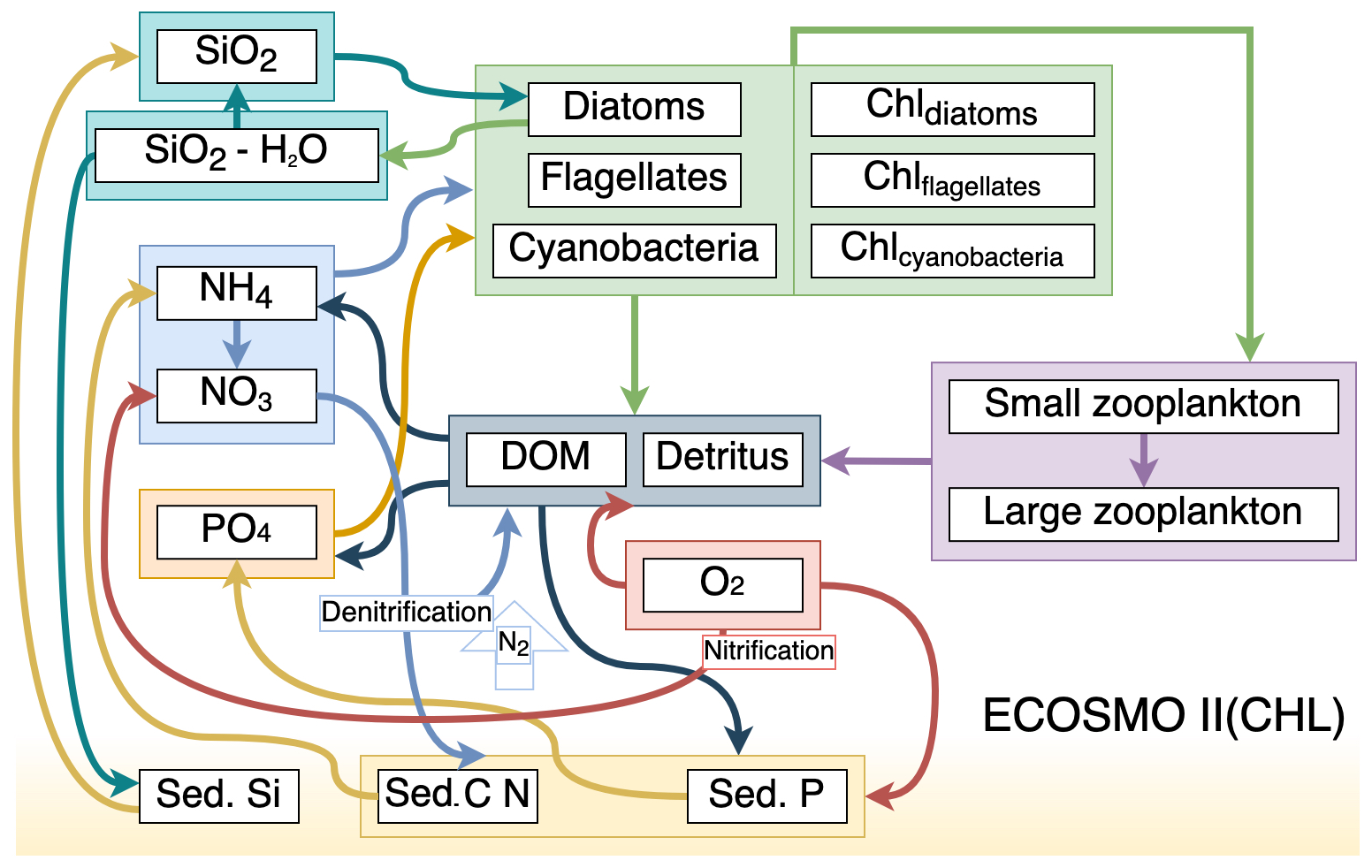
Figure 2Schematic diagram (after Yumruktepe et al., 2022b) of biochemical interactions in ECOSMO II(CHL) (DOM: dissolved organic matter; Chl prefixes stand for phytoplankton-type-specific chlorophyll a content; Sed. denotes a sediment pool with silicate, phosphorus and nitrate contents).
ECOSMO II(CHL) version Y2022 represents the current (December 2022) operational marine biogeochemical model for the Nordic seas and the Arctic Ocean (ARC MFC – Arctic Marine Forecasting Centre) under the umbrella of The Copernicus Marine Services (https://marine.copernicus.eu, last access: 22 November 2023; https://doi.org/10.48670/moi-00003, Copernicus Marine Service, 2023). This model's formulation and its parameterization were used as the reference model (referred to as “REF”) for the experiments conducted in this study. While Y2022 presents upgrades to the DS2013 version with the addition of an explicit chlorophyll a variable for each phytoplankton functional type, an evaluation of the model by Yumruktepe et al. (2022b) revealed that further refinement of the chlorophyll a is needed to improve its dynamical response to varying light conditions. We address this issue while presenting the use case of the along-track BGC-Argo modelling framework. Thus, we have introduced changes to the light limitation on phytoplankton growth formulation and to various parameters, and these changes will be validated using the BGC-Argo data.
ECOSMO II(CHL) formulates the biological interactions for phytoplankton types and chlorophyll a for P1 and P2 (diatoms and flagellates respectively) as follows:
where
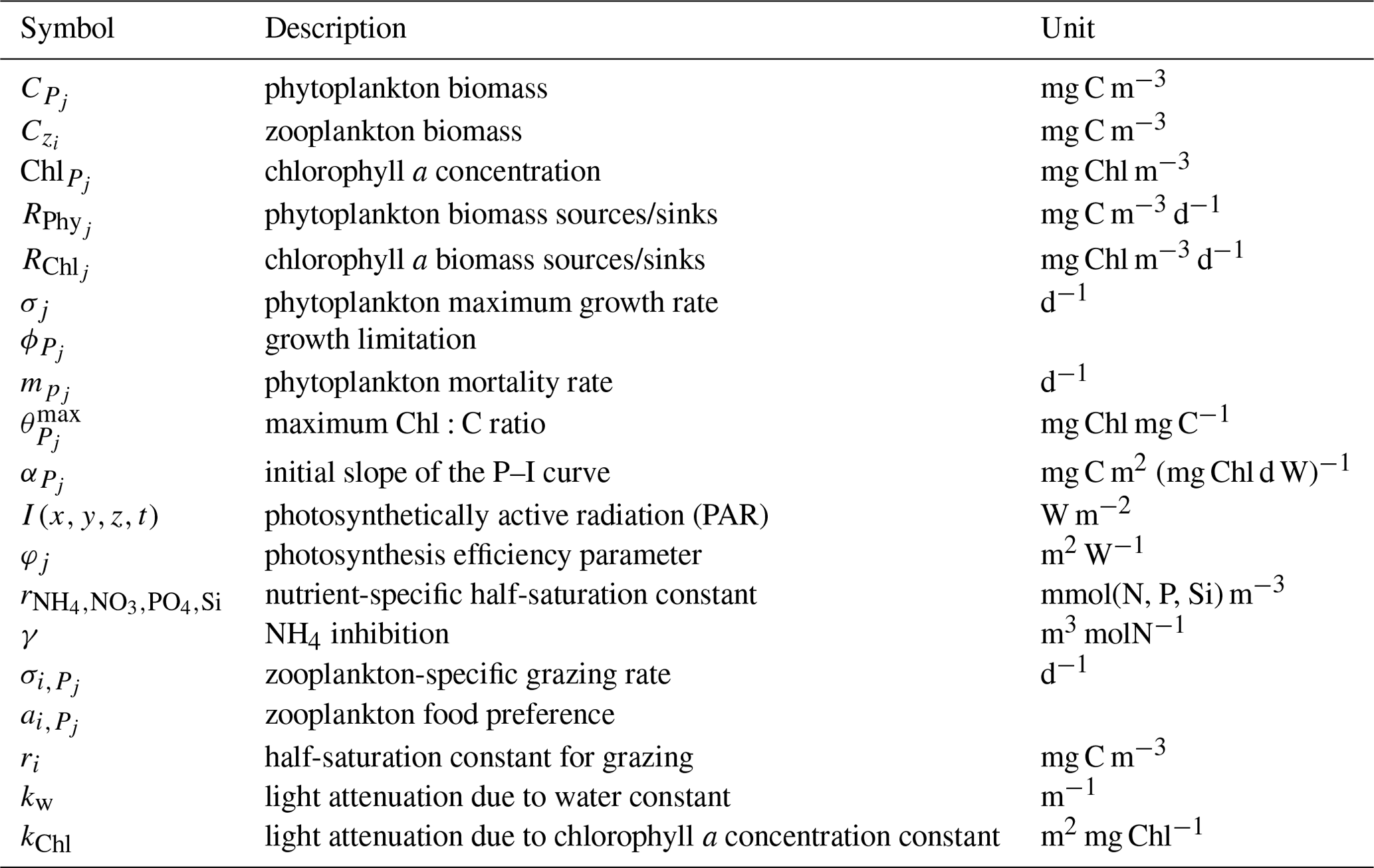
with j=1, 2 denoting the specific phytoplankton types and i=1, 2 denoting the specific zooplankton types. P (phytoplankton) and Z (zooplankton) concentrations in mg m−3 are represented by C, while Chl denotes the chlorophyll a concentration in mg m−3. Silicate is not included in the flagellate equations. The parameter definitions and units are provided in Table 1. Photosynthetically active radiation (PAR) is defined as and formulated as
j=1, 2 denote the specific phytoplankton types and i=1, 2 denote the specific zooplankton types. Please refer to Yumruktepe et al. (2022b) and Daewel and Schrum (2013) for the parameter values that are not given in Table 2.
While chlorophyll a was introduced as an explicit variable in Y2022, its effect on phytoplankton growth was only indirectly included through Eq. (17) as a self-shading parameter that affects light attenuation. Variability under varying light conditions was allowed by defining the C:Chl ratio as a function of light (Eq. 7). In this study, we expand on the Y2022 approach and assume that chlorophyll a has a direct effect on phytoplankton growth, e.g. low-light conditions trigger a higher production of chlorophyll a (present in Y2022) and will increase production (introduced in this study) as the higher chlorophyll a concentration resembles an increased use of light energy. This was achieved in experiments (denoted “EXP”) by modifying αj(I) in Eq. (9), the light limitation on growth, according to the formulation of Evans and Parslow (1985) and the parameterization of Bagniewski et al. (2011):
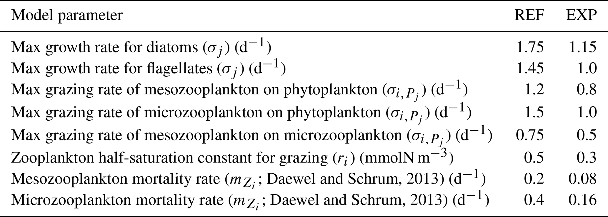
Following these changes, the chlorophyll a concentration has a direct influence on phytoplankton productivity, and our initial experiments suggested that the model was too productive compared to the observed values obtained from BGC-Argo profilers (results not shown) when using the REF parameterization set. For this reason, the parameters relating to productivity, such as growth and grazing rates, were modified in the EXP simulations to keep the primary production level comparable with the observations. The new values (Table 2) are similar to those given in Daewel and Schrum (2013). The changes can be summarized as decreases in the phytoplankton growth rates, decreases in the grazing rates to reduce the pressure on phytoplankton with the new lower growth rates, and reductions in the zooplankton mortality rates to balance the reduced grazing rates. For more details on the use of these parameters, see Sect. 3.3.2.
Daewel and Schrum, 2013Daewel and Schrum, 2013Table 2Comparison of ECOSMO II(CHL) parameters used in the REF and EXP configurations.
2.4 Along-track modelling setup
2.4.1 Preparation of forcing files
Along-track BGC-Argo modelling was conducted on eight BGC-Argo trajectories. One experiment was performed separately for each trajectory, and the models were configured in separate folders. Several criteria were involved in the choice of trajectories suitable for the modelling experiments. (1) The resolution of the BGC-Argo chlorophyll a data had to be sufficient to represent temporal variations and high-resolution changes at depth in order to validate the model chlorophyll a. In the case of temporal resolution, Silva et al. (2021) gives a range of 28–58 d for the duration of the spring bloom for the Norwegian and Barents seas. It is highly unlikely that conventional on-board in situ observations could provide the samples to cover the onset, peak and decay of the spring bloom within a large regional area, whereas with a sampling frequency of 5–10 d, BGC-Argos can capture the changes for the duration of the spring bloom in the Nordic seas. BGC-Argo buoys with long gaps in time were either avoided or the years with missing data were not included in the experiment. (2) BGC-Argo buoys that were sampling a continuous and similar water mass in the same region during their courses were selected to construct suitable environmental conditions for the model (e.g. the nutrient, temperature and salinity climatology). (3) BGC-Argo buoys with at least 1 year of time-series data were chosen to represent a full-year cycle, and buoys with multiple years were prioritized. (4) Although the Norwegian Sea is given priority, buoys from other regions such as the south of Greenland or the North Atlantic Subpolar Gyre were selected for wider regional coverage. If a subsection of the whole BGC-Argo trajectory fitted those criteria, only that time frame was included in the model.
We set the model's initial conditions using profiles representative of the BGC-Argo location data for both the physics (temperature T and salinity S) and nutrients (nitrate, silicate and phosphate). WOA18 monthly nutrient, temperature and salinity were retrieved from the closest location to the buoy coordinates at the start of the simulation. A monthly time-series text file indicating year, month and the 15th day covering the years 2000–2020 was prepared for each nutrient, temperature and salinity variable. The model automatically interpolated the data to the exact date of the model time. WOA18 data files were set to cover the whole water column. For each T and S profile, values for the upper 1000 m (for which there was the most coverage and continuity) were taken from BGC-Argo buoys, whereas those for depths below 1000 m were copied from WOA18 data interpolated to the exact coordinates of the buoy and date. This was to ensure that realistic environmental conditions were present prior to the model spin-up. World Ocean Atlas 2018 (WOA18; Boyer et al., 2018; Locarnini et al., 2019; Zweng et al., 2019; Garcia et al., 2019a, b)) monthly climatology for temperature, salinity, nitrate, silicate, phosphate and oxygen was used as the initial conditions and monthly relaxation data.
The high-resolution (1 h) ECMWF Reanalysis v5 (ERA5; Hersbach et al., 2020) was used to construct the atmospheric forcing along the buoy trajectory in order to replicate the physical conditions at the ocean surface, and the surface short-wave radiation was included as an atmospheric forcing to drive the primary production by the phytoplankton. The latitudes and longitudes of the buoys were linearly interpolated to 1 h intervals to precisely locate the closest point with atmospheric data for each forcing. The ERA5 products used to construct the atmospheric forcing were (1) the total cloud cover, (2) the mean total precipitation rate, (3) the mean surface net short-wave radiation flux, (4) the mean sea level pressure, (5) the 2 m temperature, (6) the 2 m dew-point temperature, and (7) the 10 m U and V wind components. These datasets were stored in a text file with a column for each and an extra column for the time variable.
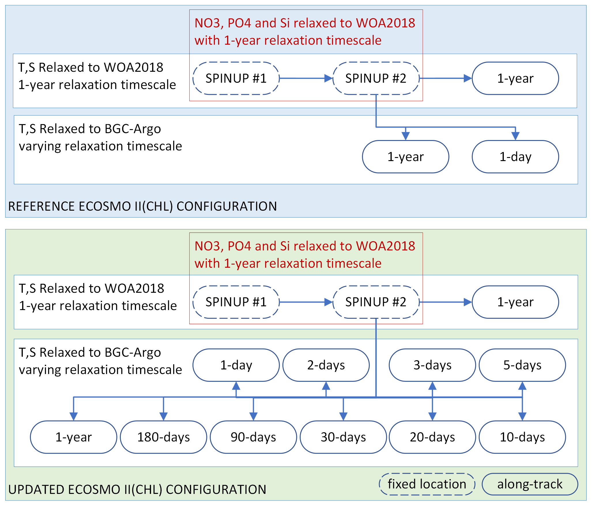
Figure 3Summary of the two sets of simulations: (1) those using the reference ECOSMO II(CHL) configuration (REF, blue box) and (2) those using the updated ECOSMO II(CHL) configuration (EXP, green box). The experiments relied on temperature (T) and salinity (S) relaxation to either WOA2018 or BGC-Argo data with varying relaxation timescales, where the spin-up simulations were relaxed to WOA2018 T and S at a fixed location (which was the initial point in along-track simulations). Along-track simulations were conducted in parallel using the final day of spin-up #2 as the initial conditions. Spin-up simulations were also relaxed to WOA2018 NO3, PO4 and Si with a 1-year relaxation timescale. No nutrient relaxation was applied to along-track simulations.
2.4.2 Model experiments
We experimented with two versions of ECOSMO II(CHL), REF and EXP, with three generic sets of simulations for each: (1) spin-up (“spinup”), (2) along-track relaxation to the climatology (“WOA”) and (3) along-track relaxation to BGC-Argo (“Argo”). Each BGC-Argo track modelling experiment involved the common set of simulations depicted in Fig. 3.
An along BGC-Argo track experiment started with two 8-year cycles of spin-up. The 8-year integration window was used to reduce the boundary condition size and preparation time for a longer-term atmospheric forcing. For the spin-up simulations, the model temperature, salinity and nutrients were weakly relaxed to the monthly climatology (1-year relaxation timescale: 3×10⁷ s). The spin-up simulations were performed at the coordinates of the first time-step of the along-track simulations, thus establishing stable initial conditions for the model. The nutrients were relaxed to climatology values to prevent drifts during a 16-year simulation. Since the spin-up model location was common to all experiments for a particular BGC-Argo buoy, it was simulated once and the restart file was stored for the along-track experiments.
Each along-track simulation started with the initial conditions provided by the second spin-up. The along-track experiments differed from each other by the temperature and salinity datasets they were relaxed to (WOA18 or BGC-Argo) and the relaxation timescale that was used in the simulation. To prevent artificial nutrient additions, relaxation to nutrients was turned off for both the WOA and Argo simulations. Each of these experiments was identified by an abbreviation consisting of a prefix indicating the ECOSMO version, the BGC-Argo number (if necessary for the text), and a suffix indicating the dataset it was relaxed to and the simulation's relaxation length scale (e.g. REF-6902547-WOA-1year or, in short, REF-WOA-1year when it is obvious from the text that the BGC-Argo number is 6902547).
The concept behind the experiment setup depicted in Fig. 3 is as follows:
-
The experiments are divided into two major groups: (1) REF, which use the reference ECOSMO formulation and the parameterization of Yumruktepe et al. (2022b), and (2) EXP, which use the final formulation and the parameterization set obtained after a series of experiments conducted during this study. The sensitivity analyses conducted to achieve the EXP parameter set is not presented here. In the following sections, the REF and EXP experiments are compared and the improvements achieved with and shortcomings of the EXP experiments are discussed.
-
Relaxing a 1D model to a climatology dataset is a very common practice. Thus, for each REF and EXP category, the WOA simulations are used as the reference simulations to evaluate the added value of relaxing the model T and S to the BGC-Argo T and S with the assumption of reducing errors in the modelled physics.
-
The Argo simulations, each of which has a unique relaxation timescale showcasing the effect of the strength of relaxation towards the BGC-Argo T and S on the biogeochemistry. Comparing each Argo simulation to the respective WOA simulation, and comparing them all, including the WOA, to the BGC-Argo chlorophyll a, yields the performance of our modelling approach along the BGC-Argo track. An analysis of the physics of the WOA and Argo simulations is performed to determine the optimal relaxation timescale as a reference for future studies using a similar approach.
-
The best-performing EXP simulation's formulation and parameterization represent the final outcome of our approach and are subjected to further testing in a 3D-modelling framework for use in a potential upgrade to the ECOSMO II(CHL) model formulation.
2.5 Model statistical analysis
When constructing the statistical evaluation of the model along the BGC-Argo track, the BGC-Argo sample points were linearly interpolated to model depth. The model and BGC-Argo data were separated into monthly and 10 m depth interval clusters. A statistical analysis was performed for each cluster, and the bias and rmse were calculated using Eqs. (1) and (2) respectively (see Sect. 3.3.3). The statistics were calculated for chlorophyll a in units of log10(mg Chl m−3).
3.1 Biogeochemical Argo data evaluation in the Nordic seas
BGC-Argo chlorophyll a data have been undergoing quality checks and adjustments (e.g. Xing et al., 2012; Roesler et al., 2017) and have improved significantly in recent years. A key adjustment is the division by 2 suggested by Roesler et al. (2017). They suggested that this division improves the overestimation of the factory-calibrated chlorophyll a seen in estimates from the WET Labs Environmental Characterization Optics (ECO) series of chlorophyll fluorometer sensors. However, this adjustment is a global average correction, whereas regional values may differ, and therefore, before progressing further with the model experiments, it is important to evaluate the BGC-Argo chlorophyll a data for the Atlantic north of 50∘ N and to evaluate whether the division by 2 is also valid for that region.
Evaluating the BGC-Argo chlorophyll a against in situ data would have been the preferred choice, as these samples cover deeper layers in the water column. However, there were too few co-locations between BGC-Argo and in situ samples (Fig. 1), leading to an unreliable statistical analysis. Therefore, satellite chlorophyll a data were used as an independent cross-validation dataset, and the BGC-Argo and in situ sample chlorophyll a were separately analysed statistically against satellite data. We note that van Oostende et al. (2022) showed that there are inconsistencies in the continuity of the OC CCI v5.0 chlorophyll a product that appear as sudden steps in the time series. These steps appear when a satellite is launched or removed. For this reason, we limited our statistical analysis to the period from May 2012 to May 2016, when only MODIS and VIIRS were continuously active, as this time frame fitted our study period. Figure 1 in van Oostende et al. (2022) depicts no sudden steps in the OC CCI V5.0 data for this period.
Both visually and statistically (Fig. 4), the BGC-Argo and in situ sample chlorophyll a are generally similar to the satellite chlorophyll a. This analysis indicates that the default quality corrections applied to BGC-Argo chlorophyll a ensure a good representation of the in situ sample chlorophyll a while noting that the satellite data are limited to the optical depth at the surface. Unfortunately, we do not have the required data at depth to compare the BGC-Argo data to, and we rely on the quality information document for the reprocessed in situ observations (Jaccard et al., 2018). Following this evaluation, we conclude that the BGC-Argo chlorophyll a dataset is of sufficient quality to be used as a validation tool for biogeochemical models for the Nordic seas without any further post-processing. This evaluation ensures that we can proceed with the modelling experiments.
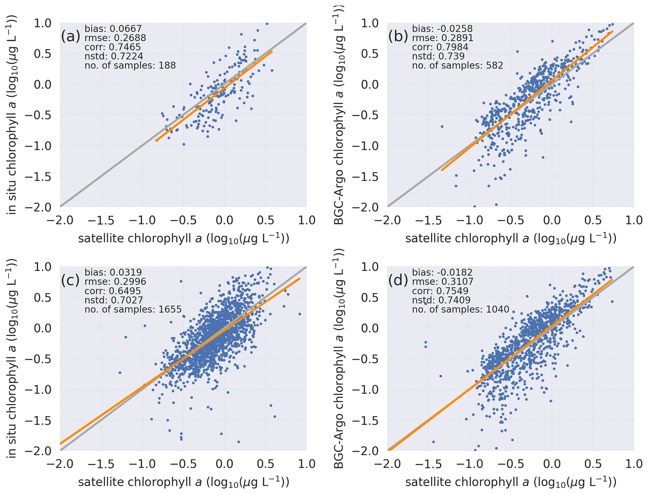
Figure 4Statistical analyses of chlorophyll a based on in situ bottle samples with search radii of (a) 2 km and (c) 10 km and BGC-Argo with search radii of (b) 2 km and (d) 10 km reveal that a comparison of BGC-Argo statistics against satellite chlorophyll a shows the same pattern as a comparison of in situ bottle statistics against satellite chlorophyll a. The computed statistics and number of sample points for each sample set are depicted in the figures. Equations for the computed statistics are described in Sect. 2.2. Data from all sources are log10 transformed.
3.2 Along-track model physics evaluation
The model physics and variations of it stemming from different relaxation scales play a crucial role in the biogeochemistry, and we therefore evaluated the effectivenesses of the different relaxation scales at reproducing the observed temperature and salinity profiles along the tracks. By simulating temperatures and salinities as similar as possible to the observed values (within a margin that allows the model dynamics the freedom to perform properly), we establish the foundation for biogeochemical model experiments that minimize the impact of errors stemming from model physics. As a result, we can target the biogeochemistry for improvements.
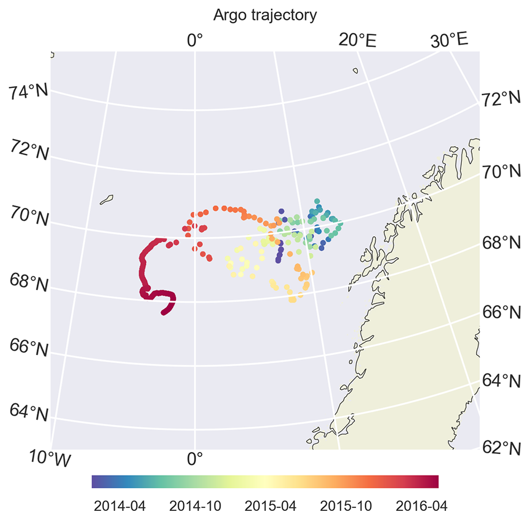
Figure 5During its drift, BGC-Argo 6902547 was confined to the Norwegian Sea and was mostly trapped in the Lofoten Basin. Later in 2016, it drifted westwards. We limit our model evaluation to the period before this, mainly focusing on 2014 and 2015.
In our approach, we considered a simulation where the model T and S were relaxed to WOA18 with a 1-year relaxation timescale (i.e. REF-WOA-1year) as the typical setup for a 1D simulation, so this can be considered a reference experiment. This is the case for both the model physics and the biology. The remaining experiments (i.e. REF-Argo-“relaxation_scale”) are iterations that allow us to evaluate the optimal relaxation timescale for progressing with the biogeochemical experiments. The simulations REF and EXP can be used interchangeably as they both use the same physics.
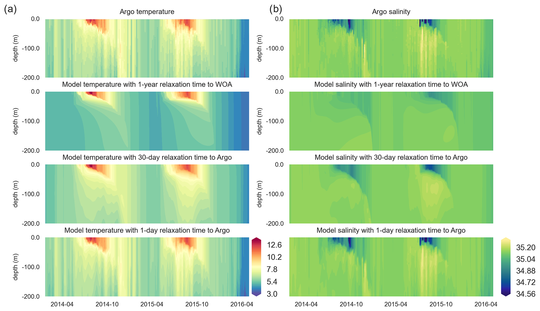
Figure 6Along-BGC-Argo 6902547-track vertical temperature (a) and salinity (b) Hovmöller plots depict increasing similarities between the BGC-Argo temperature and salinity and the modelled temperature and salinity as the relaxation timescale parameter decreases, such that they have practically identical values when a 1 d relaxation scale is used.
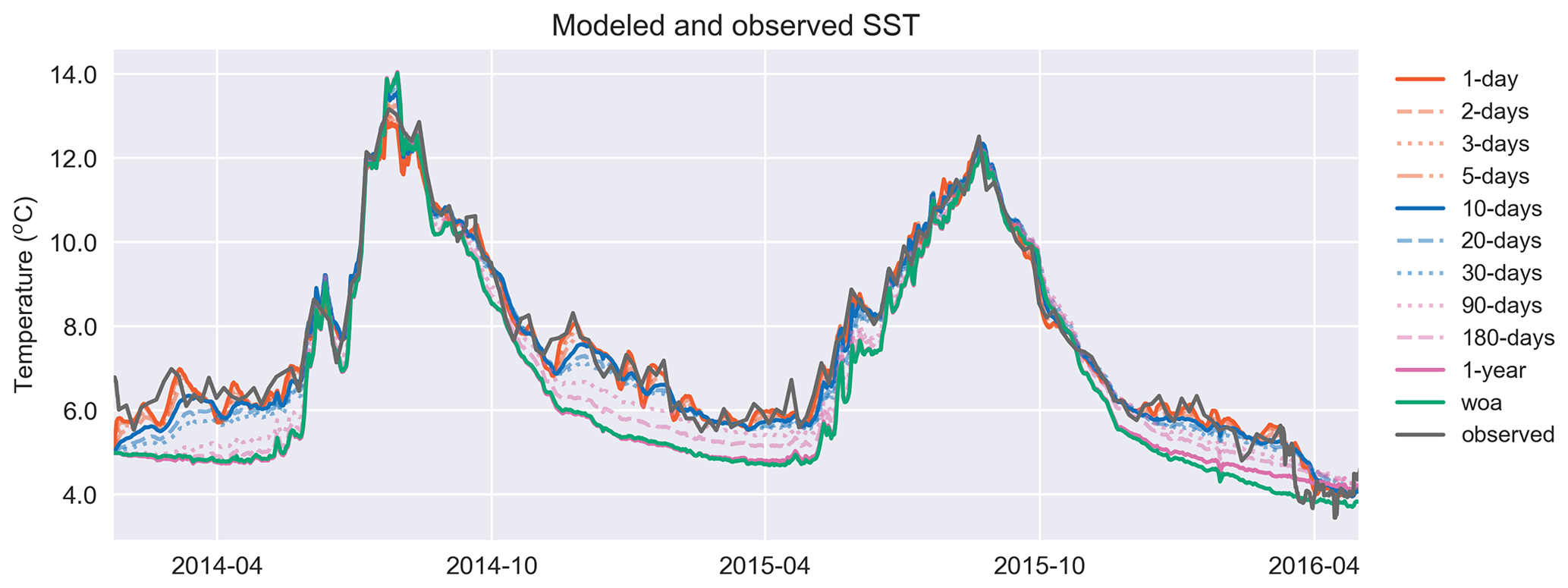
Figure 7Similar to T in Fig. 6a, the model surface temperature performs better against the satellite sea surface temperature as the relaxation scale decreases. The simulation identified as “woa” corresponds to REF-WOA-1year, and the remaining simulations correspond to REF-Argo with different timescales of relaxation.
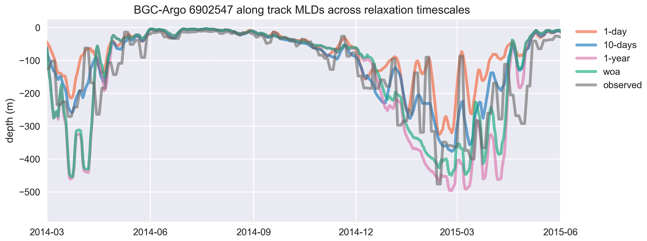
Figure 8Similar to the cases of temperature and salinity, the mixed layer depth (MLD), estimated by using a density change criterion of 0.03 kg m−3 from 10 m, is represented better in experiments that use shorter relaxation timescales. The model MLDs depicted in this figure are the GOTM model output “MLD_surf” calculated from turbulence. For visual clarity, the time period of the BGC-Argo track has been shortened, and model experiments are limited to a few representative simulations. The full time period that includes every simulation is provided in Fig. A1. The simulation identified as “woa” corresponds to REF-WOA-1year, while the remaining simulations correspond to REF-Argo with different timescales of relaxation.
We use BGC-Argo 6902547 (Fig. 5) to showcase the capabilities of the framework we designed; the figures from the other experiments are included in the Supplement. We use the BGC-Argo and satellite sea surface temperatures to evaluate the simulated temperature, salinity and mixed layer depth (MLD) from the experiments with different relaxation scales (Figs. 6, 7 and 8). For visual clarity, Fig. 8 focuses on a portion of the BGC-Argo track with a limited number of simulations. The full time period and set of simulations are depicted in Fig. A1.
Both the simulated temperature and simulated salinity (Fig. 6) become progressively more similar to the observed values as the relaxation timescale is shortened (i.e. there was a stronger influence of the BGC-Argo T and S profiles), with the simulation using WOA18 relaxation having the least short-term variability. Even in the case of 30 d of relaxation (REF-Argo-30days), temporal variability is less pronounced compared to that of 1 d of relaxation (REF-Argo-1day). An argument can be made that evaluating the model results with the dataset that it was relaxed to could raise concern, but when the simulations were compared to an independent dataset (i.e. the satellite sea surface temperature (SST; Fig. 7)), the differences between the experiments are evident, especially for the months of October–May, when vertical mixing is high. REF-WOA-1year presented the lowest performance for those months, and it required relaxation timescales of 30 d or less to achieve a better fit with the observed SST, while the short-term relaxations (1–5 d) performed better.
We focus in particular on the MLD, as it is important for controlling phytoplankton phenology (e.g. the timing, depth and duration of bloom events). All the simulations use the same atmospheric forcing, so the choices of relaxation dataset and timescales are the dominant drivers of differences in MLD. Notably, the MLDs (Figs. 8 and A1) for both cases with 1-year relaxation scales, REF-WOA-1year and REF-Argo-1year, are similar, and MLDs deeper than the observed ones are consistently calculated for these cases, especially for 2014 and the early spring of 2016. This is also evident in Fig. 7, where the SSTs for the mixing period in these two simulations are cooler compared to the SSTs in the other experiments and the observed values. Due to a better fit with the observed MLD estimate, the short-term relaxation scale experiments (30 d or less) achieve a more pronounced inter-annual variability in MLDs (e.g. shallower winter MLDs for 2014 and deeper ones for 2016). These results demonstrate that the use of Argo-driven model physics produces more optimal physics in the biogeochemical simulations. For this purpose, as we progress through the model results in the following sections, we will be focusing on those of the 1 d relaxation-scale experiments when showcasing the relaxation to the BGC-Argo experiments.
3.3 Modelled chlorophyll a evaluation
3.3.1 Evaluation of the reference ECOSMO II(CHL) formulation
We first evaluate the reference ECOSMO II(CHL) simulations in order to detect shortcomings, and later focus on these to improve the model results by objectively analysing them against the BGC-Argo chlorophyll a. Investigating this approach and its outcome is the primary objective of our study.
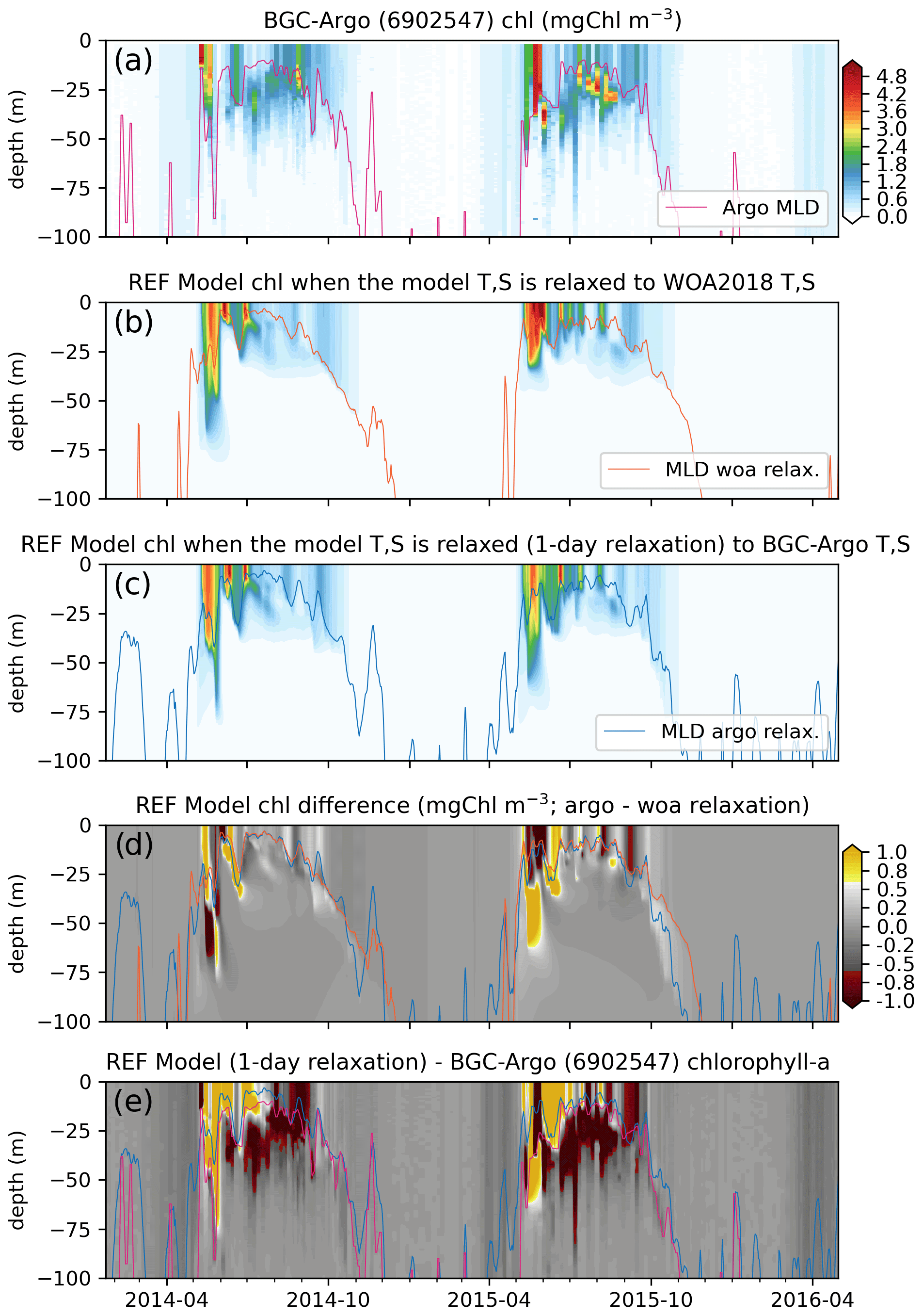
Figure 9Comparisons between the (a) observed (BGC-Argo 6902547) and the (b) REF-WOA-1year and (c) REF-Argo-1day modelled chlorophyll a reveal notable differences between the two models (d; REF-Argo-1day – REF-WOA-1year) and between the model and observed data (e; REF-Argo-1day – BGC-Argo). Note that, for panel (e), the BGC-Argo chlorophyll a was linearly interpolated to the model depth points.
We present the observed (Fig. 9a) and simulated (REF-WOA-1year and REF-Argo-1day; Figs. 9b and c respectively) chlorophyll a along the same BGC-Argo trajectory described in Sect. 3.2. We used REF-Argo-1day for this comparison since the MLD, T and S were better represented with a short-term relaxation timescale (Figs. 6, 7 and 8). Investigating the optimal timescale for relaxation (see Sect. 3.4) reveals that 1 d relaxation provides the best results statistically, although differences between the short-term (1–10 d) relaxation timescales are minor and are subject to the requirements of the modelling study.
The observed chlorophyll a shows relatively minor increases in concentration (<0.5 mg Chl m−3) in early March for the 3 years, with the first peak bloom of the year occurring during early May. The first peak in 2014 was followed by a decrease in concentration and then a second (albeit weaker) peak in late June 2014. Following the second peak, the data show the formation of a deep chlorophyll a maximum (DCM) at around 20–50 m depth. A comparable second peak in June 2015 was not observed, but a DCM layer formed at similar depths to the layer that formed in 2014. The formation of the DCM started earlier in 2015. For both 2014 and 2015, a late-summer (September–October) increase in chlorophyll a concentration from the surface to deeper than 75 m was observed. During the spring bloom events, the observed chlorophyll a concentrations exceeded 5 mg Chl m−3, and, in the case of 2015, DCM concentrations exceeded 4 mg Chl m−3. Such continuous and high-resolution vertical, seasonal and inter-annual variability in the observed data showcases the unique value of BGC-Argo observations for model evaluation. Especially for the vertical case, BGC-Argo buoys are often the only available source of observations made in the open ocean.
In general, the two sets of simulated chlorophyll a, REF-WOA-1year (Fig. 9b) and REF-Argo-1day (Fig. 9c), have similar vertical and temporal patterns and concentrations. Their first peaks occur in May–June in 2014 and 2015, and those peaks are followed by lower concentrations in summer. However, there are notable differences between the two experiments (see Fig. 9d, which shows REF-WOA-1year subtracted from REF-Argo-1day). In addition, the differences are not consistent between the simulated years. The timing and depth of the differences vary between 2014 and 2015. For 2014, the REF-Argo-1day chlorophyll a concentration is higher at the surface during the spring bloom (May), while, in response, REF-WOA-1year chlorophyll a is higher below 40 m. This pattern for May–June is reversed for 2015. REF-WOA-1year chlorophyll a is higher in the 0–25 m range and REF-Argo-1day is higher below. During July in both years, REF-Argo-1day chlorophyll a is higher for the surface to 25 m depth range. After July, REF-WOA-1year simulates higher peaks in chlorophyll a concentration for this depth interval during August–September 2015. Although minor (∼0.5 mg Chl m−3), REF-Argo-1day simulates higher chlorophyll a concentrations below the MLD. The difference is prominent during October and is located as low as ∼100 m depth. Although the difference is not as prominent as during October, the REF-Argo-1day chlorophyll a is slightly higher during early May down to ∼100 m depth.
These earlier increases in chlorophyll a concentrations in May due to modified model T and S may be attributed to the earlier shoaling of the MLD in the REF-Argo-1day case (Fig. 8), which is in better agreement with the estimated BGC-Argo MLD. Shallower MLDs may decrease the light limitation on phytoplankton growth and thus conditions suitable for growth may occur earlier compared to the REF-WOA-1year case. At the end of the growth season, during October (especially in 2015), the deeper MLD in the REF-Argo-1day case (in better agreement with the estimated BGC-Argo MLD) allows for greater intrusion by nutrients into the nutrient-limited surface layers. This allows more productivity during these late summer periods, which is prominent in the ∼25–100 m depth range. These noted differences correspond to the changes in biology when the model T and S are altered by strongly relaxing them to the BGC-Argo T and S, and they showcase the changes in biology that occur when only the model physics is changed.
After minimizing the model physics errors and the resulting errors in biology, we can identify and target the differences between the simulated and observed chlorophyll a. To identify the differences, we compare the estimated chlorophyll a of the REF-Argo-1day simulation to the observed chlorophyll a from BGC-Argo. In a similar fashion to Fig. 9d, the observed chlorophyll a is subtracted from the REF-Argo-1day chlorophyll a (Fig. 9e). With this comparison, we detect important patterns of differences: (1) the model fails to reproduce a distinct deep chlorophyll maximum (DCM) as the difference is always highly negative throughout June–September in the 20–50 m depth range (and sometimes as deep as 75 m) and highly positive near the surface, and (2) the timing of spring bloom initiation is late, as the difference is small and negative during April–May, which is consistent with the simulated shallower MLD during this period.
3.3.2 Phytoplankton growth formulation and parameterization
Prior to discussing the changes to the model, it is important to elaborate on the effect of the uncertainty of the BGC-Argo data, as we rely on this dataset to exert changes to the model code and parameterization. As is the nature of observations, they all are different from the true value, and there will be mismatches (Skogen et al., 2021), even in the case of in situ chlorophyll a bottle samples. Nevertheless, while we acknowledge that there are mismatches between different datasets (Fig. 4), we can still retrieve enough information from the BGC-Argo dataset to detect model shortcomings and propose improvements. For example, in every case where the model was nudged towards the BGC-Argo temperature, stronger relaxations result in a better match between the model T and the SST, which is a dataset that is independent of BGC-Argo (Fig. 7). Similarly, in the case of the BGC-Argo chlorophyll a uncertainty, we are not pursuing a precise one-to-one match between the model and BGC-Argo but exploring notable differences that should be improved regardless of the concentration differences. As such, there are fundamental errors in the model that need to be addressed, i.e. the late bloom, which disrupts the timing of energy transfer to the upper trophic levels, and the absence of the DCM, which is the production that is not accounted for in the model. These fundamental dynamics are observed in the BGC-Argo data even if they may not be represented with precise accuracy. Therefore, in the experimental phase, we focus on these two issues and investigate ways to improve the mechanics of the model in general. Noting these, fine-tuning model parameters in a follow-up study would require more research on the effect of the BGC-Argo data uncertainty.
There are various hypotheses on the effect of mixing or stratification on the initiation of the spring bloom in the north North Atlantic, ranging from the “critical stratification threshold” (Sverdrup, 1953), where sufficiently abundant light due to shallower convective mixing allows the growth to exceed losses, to the “dilution–recoupling hypothesis”, where deep winter mixing dilutes prey and predators, thus decoupling phytoplankton growth and grazing loss rates by reducing encounter rates (Behrenfeld, 2010). Later during the spring stratification, phytoplankton and zooplankton recouple with enhanced growth rates due to increased light abundance and greater grazing rates due to increased encounter rates. For the Nordic seas, Mignot et al. (2016) suggests that the photoperiod (the number of hours of light experienced by the phytoplankton daily) exceeds a critical value. Common to all of these hypotheses is the idea that stratification plays an important role in phytoplankton productivity, and errors in the model physics can thus be an important source of errors in the modelled biogeochemistry. However, we have shown the reduction in model physics errors achieved by relaxing the model T and S to the observed values in Sect. 3.2 and documented the changes in biogeochemistry in Sect. 3.3.1. This suggests that the major source of error in phytoplankton growth is related to the biogeochemical model.
Also common to all these hypotheses is the critical importance of light abundance. Even in the case of Behrenfeld (2010), which focuses more on prey/predator interactions, light has a central role. During periods where phytoplanton are decoupled from zooplankton, the phytoplankton are still dependent on light to sustain growth. However, neither REF-WOA-1day nor REF-Argo-1day simulations reproduce the winter biomass detected by BGC-Argo (Fig. 9a and e). Both the late bloom and the absence of a DCM suggest that the modelled phytoplankton growth is too low under low-light conditions. This evidence is supported by the model growth limitation results (Fig. 10), which show that the growth is light limited during low-light conditions.
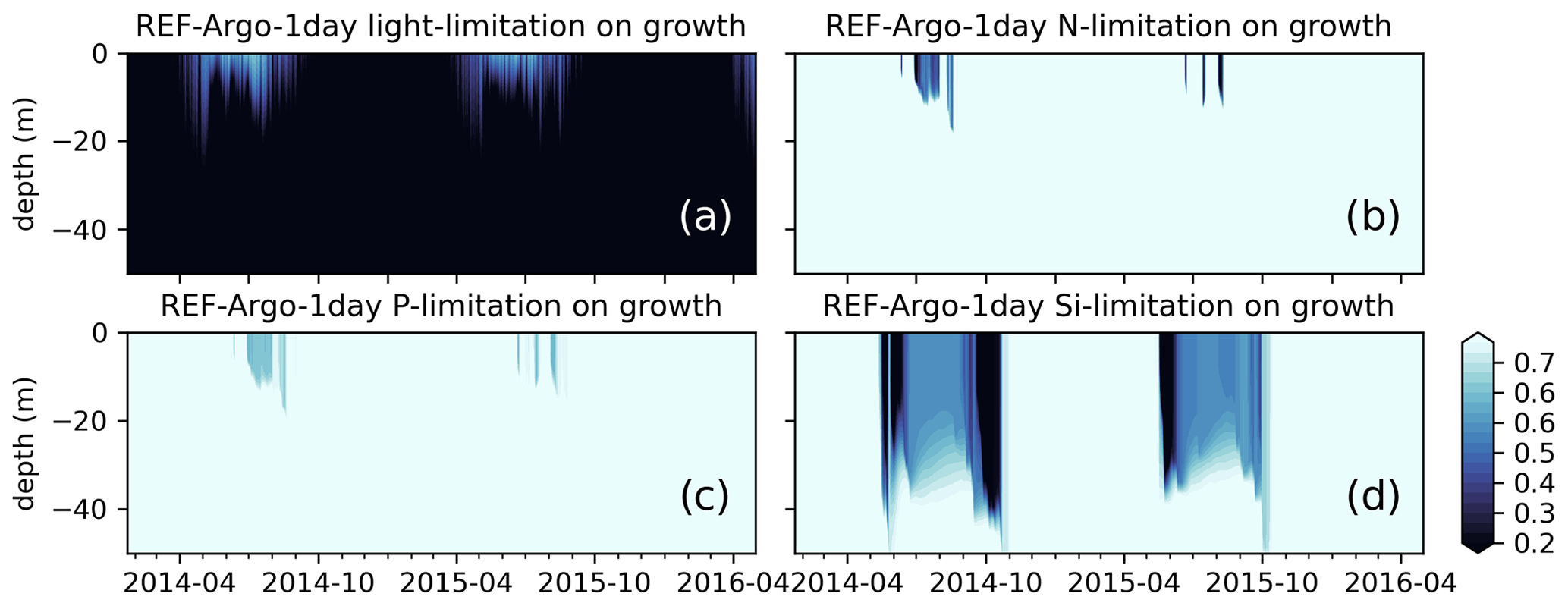
Figure 10Simulated limitations due to (a) light, (b) nitrogen, (c) phosphate, and (d) silicate on growth show that the model is mostly light limited, which can partly explain the low chlorophyll a below the surface during early spring or summer. The BGC-Argo chlorophyll a (Fig. 9a) forms a DCM in the 15–50 m depth range during the summer months, whereas the model is light limited for this depth interval. The model effectively simulates silicate limitation during the spring and late summer blooms, allowing a switch in dominance from diatoms to flagellates (results not shown). During summers, surface layers are nutrient (mainly nitrogen) limited. Note that, although the limitation on growth is a value between 0 and 1, for visual purposes we have limited the colour range to 0.25–0.75. Darker colours suggest limitation.
A prime candidate for growth limitation due to low light could be high light attenuation, but this is unlikely in the present case as the low growth occurs throughout the year; hence, in the case of a late bloom, there is not enough phytoplankton to cause excess self-shading. This suggests that the model phytoplankton are not optimally utilizing the available light (PAR). The default (REF experiments) ECOSMO II(CHL) formulation for light limitation (Eq. 9) defines the light limitation as a hyperbolic tangent curve with a photosynthesis efficiency multiplier. This function is later multiplied by the maximum growth rate, but it does not introduce variability in various conditions (e.g. light intensity, internal cellular structure). The strength of growth is moderated by the efficiency constant, which can increase/decrease the productivity as a whole rather than introducing seasonality or variations at different depths.
To achieve a certain level of variability in the EXP simulations, we have introduced a more dynamic light limitation on growth (Eq. 18) that takes into account the C:Chl ratio, which is defined as a function of light intensity. This formulation introduces enhanced productivity in the case of high intra-cellular chlorophyll a content, which the model reproduces for low-light conditions. By introducing this functionality, we disrupted the fine balance of the model parameterization, and we therefore needed to modify some of the parameters related to phytoplankton growth and, in turn, the grazing rates. The aim with this study is not to fine-tune the model parameters but to showcase the ability to use the BGC-Argo buoys as tools for model improvements. Fine-tuning the model parameters requires a cluster of model experiments and multi-regional representations, whereas we focus on a limited number of BGC-Argo tracks here. We have performed a series of experiments on model parameters to present the value added to the model and show how the model can be objectively validated using the BGC-Argo data. Table 2 summarizes the changes to the parameters which lead to a decrease in the maximum phytoplankton growth rate. We decreased the grazing pressure of the zooplankton on the phytoplankton to balance this change. Due to the lower zooplankton food intake, we also decreased their mortality rate to sustain the zooplankton biomass.
3.3.3 Evaluation of the updated ECOSMO II(CHL) formulation
The results for the experiments described in Sect. 3.3.2 are presented in Fig. 11. The simulated chlorophyll a (Fig. 11a) shows bloom initiation in April for both 2014 and 2015, with peak concentrations reached in May, followed by consecutive decreases and increases in concentration at the surface throughout the summer and prominent DCMs within the 20–50 m depth interval during July–September. Similar to the previous simulations, after the DCM period, with the increase in MLDs, late summer peaks occur as deep as 75 m in October. At its highest, the chlorophyll a concentration is ∼5–6 mg Chl m−3.
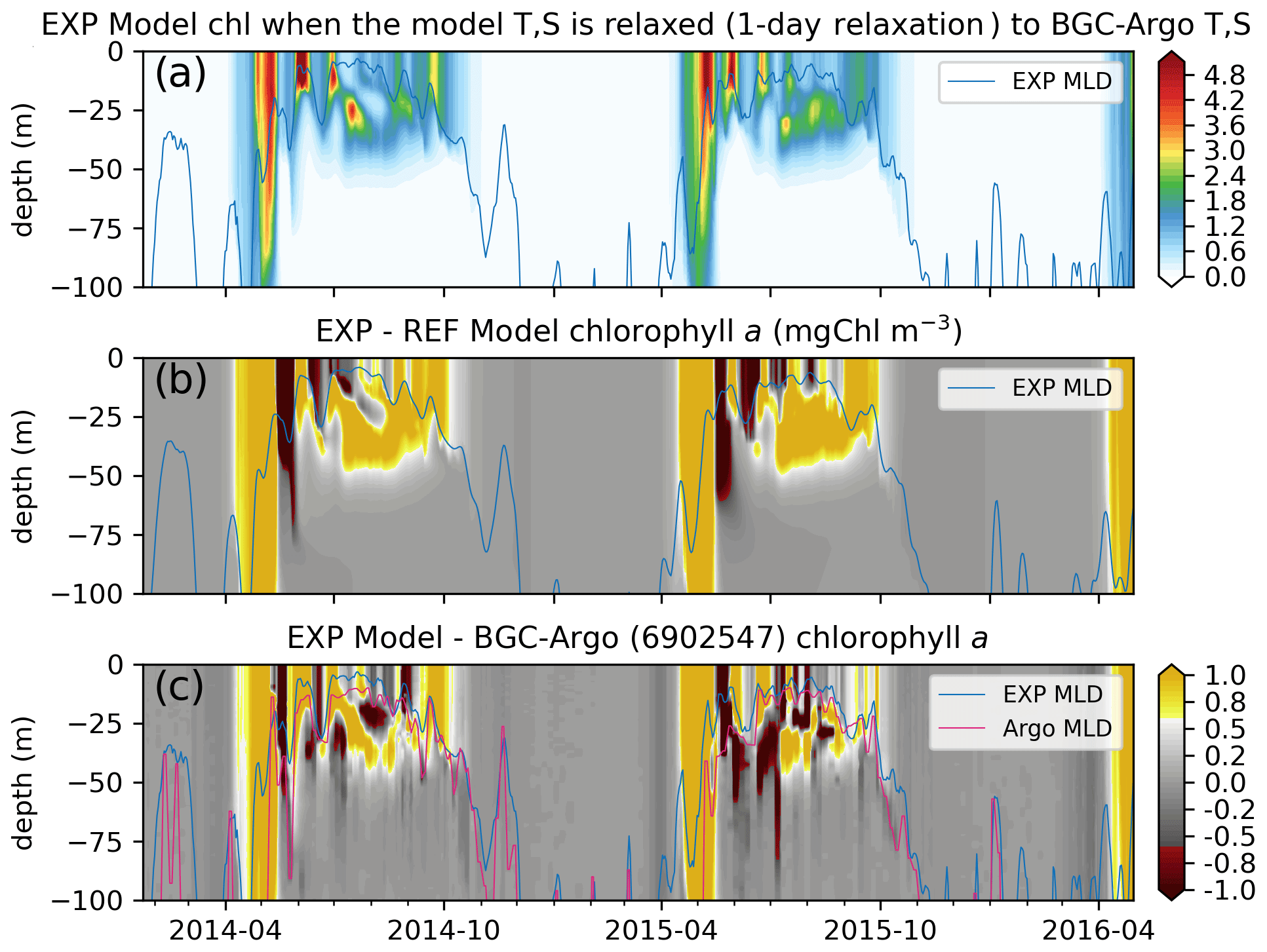
Figure 11The chlorophyll a simulated by the updated ECOSMO II(CHL) formulation (a, EXP-Argo-1day) is notably different to (b) REF-Argo-1day. The updated formulation improves the timing of the spring bloom and the summer DCM formation, as the simulated chlorophyll a is higher during these events. The opposite patterns shown in Fig. 9e (i.e. the modelled chlorophyll a is higher at the surface and lower below, suggesting the absence of a DCM) are weakened with the updated formulation; the difference between the simulated and observed chlorophyll a (c) depicts (c) local highs and lows at the observed DCM depth. The differences are also reduced for the spring bloom period, suggesting an earlier simulated bloom, which is an improvement in the model. Note that, for panel (c), BGC-Argo chlorophyll a was linearly interpolated to the model depth points, so its vertical resolution was decreased.
While, in general, the simulated chlorophyll a is similar to that described in Sect. 3.3.1, there are notable structural differences between EXP-Argo-1day and REF-Argo-1day (REF-Argo-1day is subtracted from EXP-Argo-1day in Fig. 11b): (1) the initiation and the peak of the spring bloom occur earlier, and (2) the summer subsurface chlorophyll a is more prominent in the EXP-Argo-1day simulation. As the spring bloom occurs earlier, the grazing pressure and the nutrient limitation (not shown) also initiate earlier. Both increasing the grazing pressure and increasing the nutrient limitation result in a decreased chlorophyll a concentration. During the chlorophyll a concentration decrease in EXP-Argo-1day, REF-Argo-1day is experiencing its peak bloom. This misalignment in the chlorophyll a concentration peaks indicate consecutive high positive or negative differences (Fig. 11b). Similar positive or negative differences appear throughout the summer at the surface, suggesting that the phytoplankton growth versus loss imbalance has shifted to occur earlier, resulting in mismatches in local peak concentration timings. During July–September, EXP-Argo-1day simulates higher chlorophyll a levels below the surface (20–50 m), along with lower values towards the surface, suggesting the presence of a DCM. The late-summer surface chlorophyll a concentrations are also higher in EXP-Argo-1day.
The differences between EXP-Argo-1day and BGC-Argo chlorophyll a (BGC-Argo is subtracted from EXP-Argo-1day in Fig. 11c) suggest that the applied changes do not perfectly fix the model. The results still depict differences at the highly positive or negative ends. However, when comparing them to the differences between REF-Argo-1day and BGC-Argo (Fig. 9e), we can see that the high negative bias throughout June–September for the 20–50 m depth range (see Sect. 3.3.1) is reduced, as Fig. 11c depicts highs and lows for the 20–50 m depth interval which indicate increased phytoplankton growth at lower light conditions. For better accuracy, the timing of peak concentrations in the DCM layer should be improved when tuning the model parameters in the future.
In addition to the visual comparison, the statistical analysis provides an objective evaluation of the model results (Fig. 12). The high model bias and rmse during March–April are significantly decreased in the EXP-Argo-1day simulation, which can be attributed to an earlier bloom (in better agreement with the observed values). Similarly, the subsurface bias and rmse are improved during July–October, especially below 50 m. These improvements suggest that the model is now able to represent effective growth during low-light conditions because the bias improvements for the highly negative ends show that the previously very low chlorophyll a concentrations are increased under low-light conditions, which was our primary target for model improvement.
The simulated chlorophyll a still has flaws, including occasionally being too high. For example, although the timing of the spring bloom has improved, the peak concentrations are high for April–May (Fig. 11c). The late-summer concentrations during September–October are also high, which is more pronounced in 2014. Although the model occasionally produces higher DCM concentrations, those differences can be partially attributed to the dislocated depth positioning of the observed DCM. For example, during July–August 2014 (Figs. 9a and 11a), the observed DCM location ascends from below 25 m to above it, whereas the model DCM location descends from above 25 m to below it. The model does not produce a DCM during mid-June to early July 2015, thus leading to a negative difference. However, similar to the case in 2014, from mid-July to September there is a mismatch in the depth location of the DCM. Apart from these major differences, the model has shifted from a negative bias at the surface to a positive bias (which is more prominent within 0–40 m).
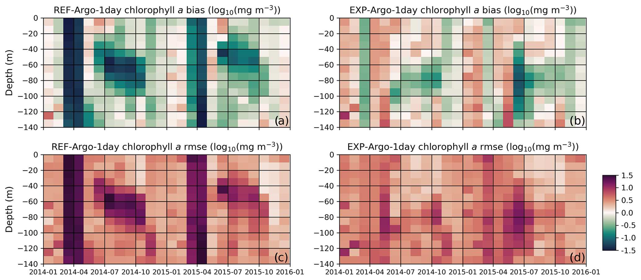
Figure 12The reference model bias (a) is improved upon by including chlorophyll a in the light-limitation function; in a light-limited environment, the model produces a lower C:Chl ratio, effectively decreasing the light limitation on phytoplankton growth rates. The bias obtained with the modified model (b) shows the greatest improvements in conditions where the light is limited, such as during the winter and early spring or at the subsurface in the summer period. Similarly, compared to the rmse for the reference model (c), the rmse for the modified formulation (d) shows the greatest improvement under the aforementioned conditions. To construct these statistics, the BGC-Argo sample points were linearly interpolated to model depth and monthly averages were taken at 10 m intervals along the water column. The statistics were calculated for chlorophyll a in [log10(mg Chl m−3)] units.
To improve the clarity of our experimental study and the reasoning behind our thought process, we have focused only on BGC-Argo 6902547 in the main text of this paper. This allowed us to present how one can approach our framework for model evaluation and improvement. However, an argument can be raised that our changes to the model formulation and parameterization are case specific, i.e. they only apply to BGC-Argo 6902547, which was located in the Norwegian Sea between 2014–2016. In response to this argument, we point out that we targeted the phytoplankton growth under low-light conditions, as we concluded this was necessary for the model based on what the experiments revealed (see Sect. 3.3.2). The parameter changes given in Table 2 represent parameter tuning to adapt the model to its new formulation for growth. Thus, although the prescribed parameters target the specific case of BGC-Argo 6902547, the formulation change for low-light conditions should benefit the model in general, which was the case in other experiments we conducted in this study. We did not include the results of those experiments here, but the alternatives to Figs. 6, 7, 8, 9, 11 and 12 for each specific experiment are provided in the Supplement. All reference experiments (REF simulations) were mostly light limited, whereas every modified model experiment (EXP simulations) showed objectively improved results for light-limited conditions according to the assessment statistics (see the Supplement).
These experiments were not only located in the Norwegian Sea; they covered various regions in the northern North Atlantic (Fig. 1), showing that the changes can improve modelling results throughout the northern North Atlantic, which is the main region that ECOSMO II(CHL) was actively developed for (Yumruktepe et al., 2022b). As discussed above, fine-tuning is necessary, as the model is too productive, which is also the case for other experiments presented in this study. However, the fine-tuning of the parameters is beyond the focus of this study, as it requires detailed sensitivity analyses. Here we have focused on building a framework where BGC-Argo can be easily used for driving the model physics and, at the same time, provides a high-resolution dataset for its evaluation. This paper is an example of how one can approach this framework. A follow-up study is needed to fine-tune the model parameters using multiple BGC-Argo tracks (and to update the number of tracks with the most recent BGC-Argo deployments) in order to support model improvements in a 3D-model domain.
3.4 Discussion of the relaxation timescales
An important issue which we briefly discussed earlier (see Sect. 3.2) is the choice of the relaxation timescale used for T and S. Referencing the T, S and MLD comparisons (Figs. 6, 7 and 8), we settled on the use of the 1 d relaxation timescale, as the model physics performance was (visually) better when using a short timescale. Following up on this decision, we hypothesized that the physical correction would also lead to improved performance of the modelled biogeochemistry. It is important to objectively analyse and quantify the improvements and prove that the hypothesis is valid.
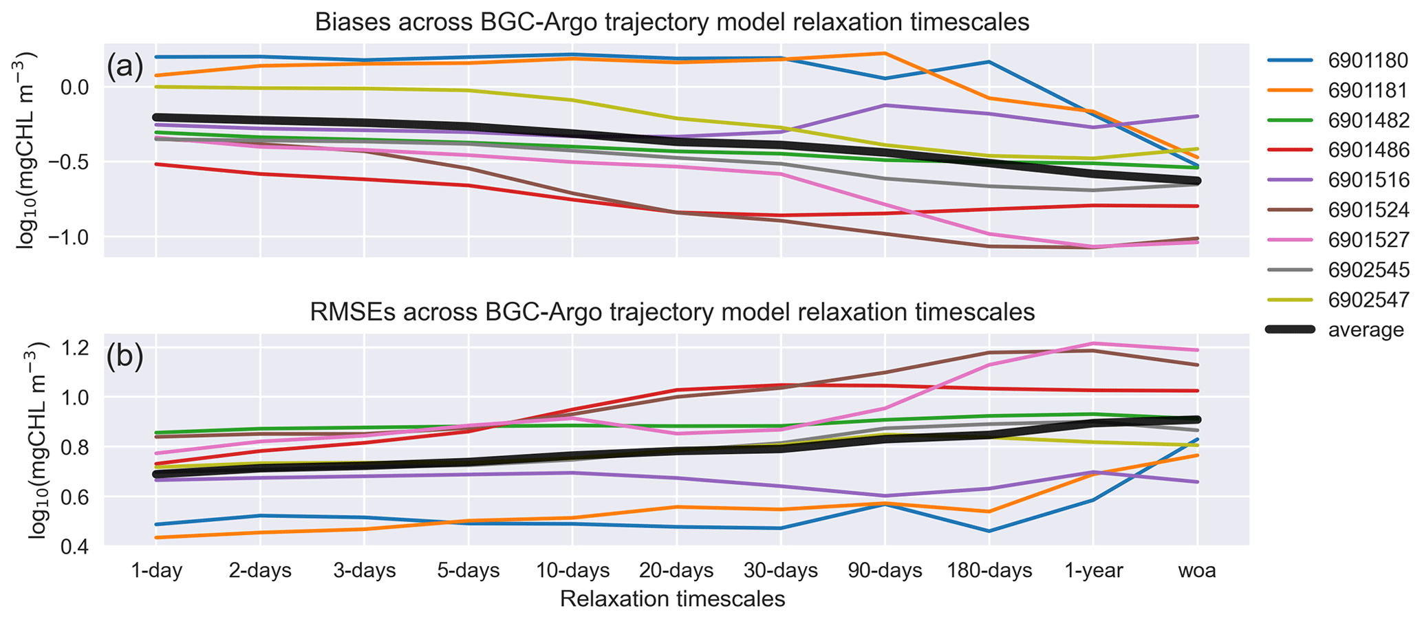
Figure 13EXP-Argo experiments: mean estimated (a) bias and (b) rmse in March–May for different timescales of T and S relaxation to BGC-Argo. All the along-track experiments show improvements to varying degrees.
The bias and rmse across the different BGC-Argo tracks used in this study for each relaxation timescale are depicted in Figs. 3, 6, 7 and 8 (Fig. 13). Since the effects of the relaxation timescales were more prominent during the winter and spring periods (Figs. 7 and 8), and since the days are short at high latitudes during winter, the statistics we present in Fig. 13 are the averages of the data points in Fig. 12 for March–May in the 0–200 m depth range. In general, Fig. 13 depicts a common pattern: as the relaxation timescale increases, the simulations become statistically less representative of the observed data, with the statistics for some BGC-Argo track experiments varying more than those for other experiments. The 6902547 case presented in detail in this study varies moderately. Since both the physics and the chlorophyll a respond more positively with shorter relaxation timescales, for this kind of approach, we suggest using a timescale that is as short as possible. We note that the differences in statistics are marginal for timescales shorter than the 10 d relaxation scale. In these cases, the scale will be decided upon based on how flexible towards the BGC-Argo T and S the model physics are intended to be. The model MLD for the 10 d scale (Fig. 8) is comparable to that for the 1 d scale.
One can argue that the statistical differences between the timescale experiments are not strikingly different, and, as such, the choice of a different timescale would be arbitrary. We argue that even if the statistical differences are relatively low for the particular case of the Nordic seas, the relaxation to climatology (WOA18) is statistically the least capable. Using climatology data, the relaxation scheme will miss anomalous events and will thus poorly represent the inter-annual variability. Capturing such variability plays an important role in understanding the ecosystem dynamics of regions where the seasonal and annual productivity is highly dependent on the strength and duration of vertical mixing events due to nutrient limitation, such as the subtropical North Atlantic (Siegel et al., 1999; Neuer et al., 2007; Helmke et al., 2010; Yumruktepe et al., 2020). Correcting the model winter physics (e.g. the timing and depth extent of the MLD and the mesoscale activity) will not only improve the model biogeochemistry in general; it will also introduce inter-annual variability.
The framework we have presented in this study may yield important applications for regions with nutrient limitation. In our case, except in the summer months, the biogeochemistry is not nutrient limited (Fig. 10b–d), and the correction we applied using the BGC-Argo physics is therefore mainly related to the light limitation and the strength of vertical mixing. While improving the strength of convective mixing, we improved the timing of the spring bloom, but the overall effect on the total productivity could be more significant in nutrient-limited regions. This hypothesis was not tested in this study, but we suggest that this would be a valuable follow-up study.
In this study, we established a 1D ocean modelling framework that employs BGC-Argo buoys for improving and evaluating biogeochemical process representations. The code we developed for this study is written in a generic format, and any BGC-Argo (or Argo if biogeochemical validation is not required) trajectory data can be used as the physical setting for a biogeochemistry simulation. The supplied code (see the “Code and data availability” section) prepares a 1D model setup by creating atmospheric forcing, climatological and Argo relaxation data along the Argo track. The framework uses the well-established GOTM physics model and The Framework for Aquatic Biogeochemical Models (FABM) biogeochemical model coupler. These allow the experiments to be set up quickly and the application of a wide range of biogeochemical models. In this study, we focused on presenting the framework, its approach and an example use case. The use case shows how the modeller can set up the experiments from scratch, so this article is also a guide to replicating similar experiments with any BGC-Argo buoy.
In addition to the presentation of technical details, we have showcased how the framework can be used to improve biogeochemical models using both the physical and biogeochemical Argo data. As our focus in this study was on presenting the technical approach, our experiments were limited to simulating the observed chlorophyll a from a limited number of buoys. Thus, immediate follow-up work to this study that utilizes the framework in a scientific focused approach is essential. We suggest extending the approach using other BGC-Argo variables such as oxygen, light, nitrate and particle backscatter. The combined use of these variables in the analyses would provide a more complete picture of light vs. nutrient limitation and the timing and depths of biogeochemical processes as well as estimates of organic matter concentrations. Such an assessment would allow for a more in-depth tuning of the model dynamics. An interesting approach would be to construct a similar study for regions where the oceanic production is highly dependent on the vertical transfer of nutrients to the surface, as improving the model physics using the BGC-Argo buoys may benefit modelling studies of regions with high nutrient limitation. A regional (or global) assessment of the biogeochemical variables using the BGC-Argo dataset (which has matured for over a decade) together with the improved models may allow an understanding of the trends in these variables.
On the topic of tuning, a planned follow-up to this study focuses on the application of more systematic parameter tuning approaches (e.g. Gharamti et al., 2017) compared to the relatively simple exercise presented here. In the future, the number of buoys that are used in the experiments should be increased, preferably establishing a region-wide sample set, and a detailed sensitivity analysis should be performed for a wider parameter set. For instance, we note that the model chlorophyll a is at the higher end with the parameter values chosen in this study (see Sect. 3.3.3). Dedicated parameter tuning approaches should consider uncertainties in the BGC-Argo data as well as the uncertainty ranges of the tuned parameters. Because this study focused on improving the model formulation (i.e. increasing growth rates under low-light conditions) rather than model parameter fine tuning, a dedicated assessment of BGC-Argo data errors was not included. To limit the effects of observation uncertainties, we only included (see Sect. 2.1.1) the “adjusted” BGC-Argo variables (i.e. temperature, salinity, pressure and chlorophyll a), which provide either a “real-time-adjusted” or a “delayed-mode” data control and correction (Bittig et al., 2019). Despite applying a level of correction, there are still observational errors present. For example, the measured ”fluorescence chlorophyll a concentration” to ”chlorophyll a pigment concentration” ratio can vary due to various factors, which can lead to an uncertainty as high as ±300 % (Roesler et al., 2017). However, some of these errors can be reduced to a maximum of 0.12 mg Chl m−3, corresponding to an average reduction of ±40 % (Johnson et al., 2017; Bittig et al., 2019). On the other hand, the BGC-Argo estimated particulate organic carbon (POC) uncertainty is lower but can be as high as 40 mg C m−3, about 50 %. In the case of oxygen, the sensors show a strong drift (on the order of −5 % yr−1 between calibration and deployment), this can be corrected (to approx. 1.0–1.5 µmol kg−1) with surface measurement adjustments along the track (Bittig et al., 2018). Similar uncertainties that exist for all the other BGC-Argo variables should also be accounted for in model validation studies.
We envision an ensemble simulation approach for model biogeochemical parameter tuning as a follow-up study where we construct a suite of ensemble experiments with systematic perturbations of selected model parameters within a ± uncertainty range from the respective reference parameter value. However, depending on the number of modified parameters and BGC-Argo buoys, the number of experiments can be in the thousands, which raises the question of how to select the parameter set(s) that yields the best results objectively. The statistical analyses performed in this study were done on a limited number of BGC-Argo buoys and a single biogeochemical variable (i.e. chlorophyll a), and such an analysis may give inconclusive results in a fine-tuning parameter study, given the BGC-Argo uncertainty. Newer BGC-Argo buoys are equipped with multiple biogeochemical sensors, making the statistical analysis of a parameter fine-tuning experiment more robust as the number of experiments increases while also accounting for multiple BGC-Argo variables and their associated uncertainty ranges. The inclusion of the statistics for multiple BGC-Argo variables would enhance the ecosystem representation by the parameters, and multiple variables would provide more constraints to help achieve realistic representations. At that stage of the analyses, the uncertainty ranges of the observed variables can be included, and the search for the better-performing experiments could be narrowed down for the less uncertain variables (e.g. POC, oxygen) and widened for the more uncertain ones (e.g. chlorophyll a). In addition, instead of directly incorporating the concentrations from the full experiment into the statistical analyses, valuable insights may be gained by separately assessing the timing of seasonal events driven by the mixed layer dynamics. Alternatively, comparing correlations between the model and the depth locations of key features in the BGC-Argo profiles, such as the nutricline, would give an insight to the mixing and production dynamics (e.g. Salon et al., 2019). These approaches would reduce the influence of observation errors but would rely on the consistency of the sensor along the track. Finally, a more elaborate data assimilation scheme that takes into account model variable and parameter uncertainties, such as one based on the ensemble Kalman filter, could be considered for use in this framework in an idealized setting to investigate whether or not the current model parameterization is suitable to represent the observed real-world process (e.g. Singh et al., 2022).
In parallel to fine-tuning the model parameters, it is equally important to further evaluate mechanistic approaches to phytoplankton growth, mortality, grazing pressure and organic matter export dynamics. Such mechanistic approaches allow the models to adapt to changing environmental conditions due to regional coverage, changes in climate and the state of the oceans. Our study demonstrates the possibility of designing and applying such approaches by considering (1) different regional coverages and (2) the ever-growing time period covered by BGC-Argo data, allowing us to investigate the model discrepancy at a large scale but also at the local scale when considering (3) high-resolution depth and time coverage. The study presented here is an example of the latter, as we detected a shortcoming of the simulated primary production in low-light environments and applied a mechanistic change to the model chlorophyll a dynamics with minor parameter tuning. This application was an initial attempt to showcase the utility of the framework to the wider scientific community, and a follow-up study that focuses on further mechanistic approaches is a natural extension of this study.
With this framework, we provide modellers with an alternative/additional dataset to in situ or remote sensing data, cover wider regions, depths and time periods, and, with the least effort, make these data points available for model evaluation. We envision advancements in the understanding of the functioning of marine biogeochemistry through the use of models which will be improved with the use of this framework. The cost-effective nature of this framework should allow (1) the employment of multiple models of variable complexity, (2) the application of them to various regions and time periods to cover multiple ecosystems, (3) the improvement and fine-tuning of process formulations, (4) the comparison of results for a beyond-model-specific approach, and (5) ultimately, and most importantly, the application of these models in a 3D setting to a range of use cases ranging from operational oceanography (e.g. Yumruktepe et al., 2022b) to regional or global links to higher trophic levels (e.g. Utne et al., 2012) and climate (e.g. Tjiputra et al., 2020). Through these use cases, models have the potential to be an important accessory to observations in efforts to improve our understanding of nature and the future of our oceans.
A1 BGC-Argo 6902547 modelled MLDs
This section includes the extended time period and the full set of simulations depicted in Fig. A1. The inclusion of multiple years and 12 different time series of data makes the readability of the figure challenging. However, the inclusion of each dataset in the figure is essential for achieving an understanding of the model dynamics as a response to different relaxation timescales. Therefore, we included the simpler form in the main text (Fig. 8) and provide the full set here in “Appendix A.”
A2 Observational data sources
The input files that were used for the discussed experiment in the study are archived on Zenodo; see Yumruktepe et al. (2022a). The “experiments/example” folder includes the files necessary to reproduce the experiment. The following web links are the sources of these input files, and “build_experiment.sh” in Yumruktepe et al. (2022a) is configured to connect to these links for the preparation of a new experiment:
-
World Ocean Atlas 2018, temperature:
https://www.ncei.noaa.gov/access/world-ocean-atlas-2018/bin/woa18.pl?parameter=t (last access: 7 February 2023) -
World Ocean Atlas 2018, salinity:
https://www.ncei.noaa.gov/access/world-ocean-atlas-2018/bin/woa18.pl?parameter=s (last access: 7 February 2023) -
World Ocean Atlas 2018, nitrate:
https://www.ncei.noaa.gov/access/world-ocean-atlas-2018/bin/woa18oxnu.pl?parameter=n (last access: 7 February 2023) -
World Ocean Atlas 2018, silicate:
https://www.ncei.noaa.gov/access/world-ocean-atlas-2018/bin/woa18oxnu.pl?parameter=i (last access: 7 February 2023) -
World Ocean Atlas 2018, phosphate:
https://www.ncei.noaa.gov/access/world-ocean-atlas-2018/bin/woa18oxnu.pl?parameter=p (last access: 7 February 2023) -
Ocean Colour Climate Change Initiative v5.0, chlorophyll a and kd490:
https://rsg.pml.ac.uk/thredds/catalog/cci/v5.0-release/geographic/daily/catalog.html (last access: 7 February 2023) -
BGC-Argo along-track data:
https://data.marine.copernicus.eu/product/INSITU_GLO_BGC_DISCRETE_MY_013_046/description (last access: 7 February 2023) -
ERA5 atmospheric forcing data:
https://cds.climate.copernicus.eu/cdsapp#!/dataset/reanalysis-era5-single-levels?tab=form (last access: 7 February 2023)
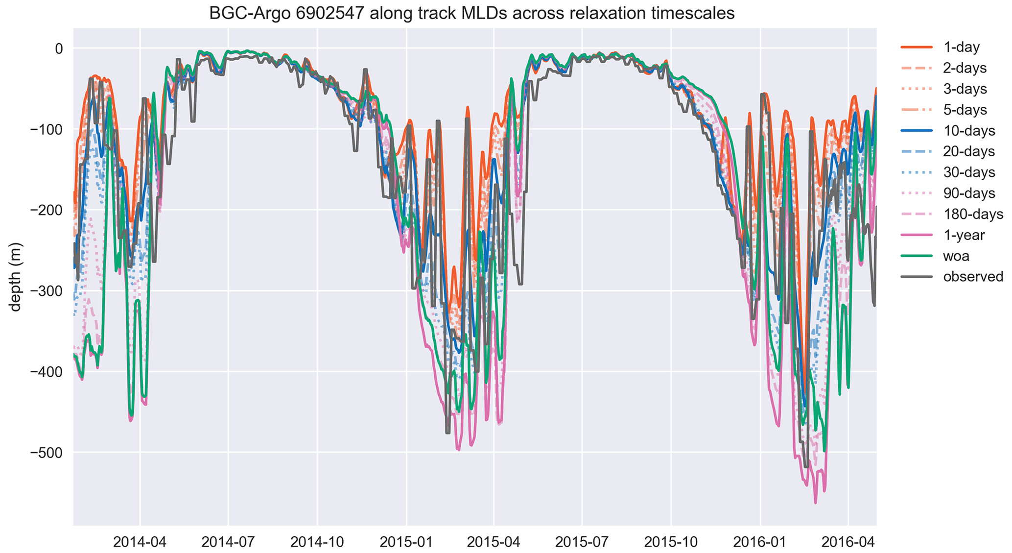
Figure A1The MLD, estimated by using a density change from 10 m criterion of 0.03 kg m−3, similar to the temperature and salinity cases, is represented better in experiments that use shorter relaxation timescales. The model MLD depicted in this figure is the GOTM model output “MLD_surf” calculated from the turbulence. This figure depicts the full time period of the BGC-Argo track and model experiments. The simulation identified as “woa” corresponds to REF-WOA-1year, and the remaining simulations correspond to REF-Argo- with different timescales of relaxation.
The exact version of the ECOSMO II(CHL) model used to produce the results used in this paper is archived on Zenodo (Yumruktepe et al., 2022a, https://doi.org/10.5281/zenodo.7773509), which includes the input data and scripts to produce the model input, run the model and produce plots for all the simulations presented in this paper. They are openly available under a Creative Commons Attribution 4.0 International license. The GOTM model and FABM coupler are developed at https://github.com/fabm-model/fabm/wiki/GOTM (last access: 24 February 2023), and the version used (GOTM version 7 revision: 2219) is included at Yumruktepe et al. (2022a) in the “gotm” directory. Yumruktepe et al. (2022a) includes a shell script, “build_gotm_fabm.sh”, that will, by default, install the GOTM-FABM version we have used in this study. The ECOSMO II(CHL) model code is written in FORTRAN. Pre- and post-processing scripts are written in Python 3. Yumruktepe et al. (2022a) includes various folders. The experiment we presented here is stored in the “experiments” folder and can be used as an example for other experiments. The “figure_codes” folder includes the scripts needed to reproduce the figures in this paper. The “nersc” folder includes the ECOSMO II(CHL) code to be coupled with FABM during compilation. “build_gotm_fabm.sh” builds the coupled GOTM-FABM-ECOSMO II(CHL). The model outputs and data used for the figures are stored in “output_files”. The main folder of Yumruktepe et al. (2022a) contains “argoinput.py”, which is a compilation of the Python subroutines that are used to build and post-process the experiments. It is recommended that you should either copy this script to your Python path or use a symbolic link where the Python scripts are executed. Investigate “README.md” for further instructions.
The supplement related to this article is available online at: https://doi.org/10.5194/gmd-16-6875-2023-supplement.
VÇY built the framework and, together with EAM, JT and AS, designed the experiments which were then carried out by VÇY. VÇY and AS are the developers of ECOSMO II(CHL). EAM and JT coupled their respective biogeochemical models to FABM (not presented here) for a follow-up work. Their experience with the coupling helped to generalize the framework code for the wider community. VÇY prepared the paper, with all co-authors providing contributions.
The contact author has declared that none of the authors has any competing interests.
Publisher's note: Copernicus Publications remains neutral with regard to jurisdictional claims made in the text, published maps, institutional affiliations, or any other geographical representation in this paper. While Copernicus Publications makes every effort to include appropriate place names, the final responsibility lies with the authors.
Model input data were stored and used through the Norwegian Sigma2 infrastructure under the project NS9481K.
This research was financially supported by the Bjerknes Centre for Climate Research projects Fast Track Initiative and The Breathing Ocean.
This paper was edited by Christopher Horvat and reviewed by two anonymous referees.
Bagniewski, W., Fennel, K., Perry, M. J., and D'Asaro, E. A.: Optimizing models of the North Atlantic spring bloom using physical, chemical and bio-optical observations from a Lagrangian float, Biogeosciences, 8, 1291–1307, https://doi.org/10.5194/bg-8-1291-2011, 2011. a
Behrenfeld, M. J.: Abandoning Sverdrup's critical depth hypothesis on phytoplankton blooms, Ecology, 91, 977–989, https://doi.org/10.1890/09-1207.1, 2010. a, b
Bittig, H. C., Körtzinger, A., Neill, C., Van Ooijen, E., Plant, J. N., Hahn, J., Johnson, K. S., Yang, B., and Emerson, S. R.: Oxygen optode sensors: principle, characterization, calibration, and application in the ocean, Front. Marine Sci., 4, 429, https://doi.org/10.3389/fmars.2017.00429, 2018. a
Bittig, H. C., Maurer, T. L., Plant, J. N., Schmechtig, C., Wong, A. P., Claustre, H., Trull, T. W., Udaya Bhaskar, T., Boss, E., Dall’Olmo, G., Organelli, E., Poteau, A., Johnson, K. S., Hanstein, C., Leymarie, E., Le Reste, S., Riser, S. C., Rupan, A. R., Taillandier, V., Thierry, V., and Xing, X.: A BGC-Argo guide: Planning, deployment, data handling and usage, Front. Marine Sci., 6, 502, https://doi.org/10.3389/fmars.2019.00502, 2019. a, b
Boyer, T. P., Garcia, H. E., Locarnini, R. A., Zweng, M. M., Mishonov, A. V., Reagan, J. R., Weathers, K. A., Baranova, O. K., Seidov, D., and Smolyar, I. V.: World Ocean Atlas 2018 [temperature, salinity, nitrate, phosphate, silicate, oxygen], NOAA National Centers for Environmental Information [data set], https://www.ncei.noaa.gov/archive/accession/NCEI-WOA18 (last access: 22 November 2023), 2018. a
Burchard, H., Bolding, K., and Ruiz-Villarreal, M.: GOTM, a General Ocean Turbulence Model: Theory, Implementation and Test Cases, Tech. Rep. Report EUR 18745, European Commission Joint Research Centre Space Applications Institute, https://op.europa.eu/s/y5wj (last access: 22 November 2023), 1999. a
Claustre, H., Johnson, K. S., and Takeshita, Y.: Observing the Global Ocean with Biogeochemical-Argo, Annu. Rev. Marine Sci., 12, 23–48, https://doi.org/10.1146/annurev-marine-010419-010956, 2020. a
Copernicus Marine: Copernicus Marine In Situ – Global Ocean – Delayed Mode Biogeochemical product, SEANOE, https://doi.org/10.17882/86207, 2023. a
Copernicus Marine Service: Arctic Ocean Biogeochemistry Analysis and Forecast, https://doi.org/10.48670/moi-00003, 2023. a
Cossarini, G., Mariotti, L., Feudale, L., Mignot, A., Salon, S., Taillandier, V., and Teruzzi, A.: Towards operational 3D-Var assimilation of chlorophyll Biogeochemical- Argo float data into a biogeochemical model of the Mediterranean Sea, Ocean Model. 133, 112–128, https://doi.org/10.1016/j.ocemod.2018.11.005, 2019. a
Daewel, U. and Schrum, C.: Simulating long-term dynamics of the coupled North Sea and Baltic Sea ecosystem with ECOSMO II: Model description and validation, J. Marine Syst., 119–120, 30–49, https://doi.org/10.1016/j.jmarsys.2013.03.008, 2013. a, b, c, d, e, f
Damien, P., de Fommervault, O. P., Sheinbaum, J., Jouanno, J., Camacho-Ibar, V. F., and Duteil, O.: Partitioning of the Open Waters of the Gulf of Mexico Based on the Seasonal and Interannual Variability of Chlorophyll Concentration, J. Geophys. Res.-Oceans, 123, 2592–2614, https://doi.org/10.1002/2017JC013456, 2018. a
Evans, G. T. and Parslow, J. S.: A Model of Annual Plankton Cycles, Biol. Oceanogr., 3, 327–347, 1985. a
Garcia, H. E., Weathers, K. W., Paver, C. R. , Smolyar, I., Boyer, T. P., Locarnini, R. A., Zweng, M. M., Mishonov, A. V., Baranova, O. K., Seidov, D., and Reagan, J. R.: World Ocean Atlas 2018, Volume 4: Dissolved Inorganic Nutrients (phosphate, nitrate and nitrate+nitrite, silicate), edited by: Mishonov, A., NOAA Atlas NESDIS 84, 35 pp., 2019a. a
Garcia, H. E., Weathers, K. W., Paver, C. R. , Smolyar, I., Boyer, T. P., Locarnini, R. A., Zweng, M. M., Mishonov, A. V., Baranova, O. K., Seidov, D., and Reagan J. R.: World Ocean Atlas 2018, Volume 3: Dissolved Oxygen, Apparent Oxygen Utilization, and Oxygen Saturation, edited by: Mishonov, A., NOAA Atlas NESDIS 83, 38 pp., 2019b. a
Gharamti, M., Tjiputra, J., Bethke, I., Samuelsen, A., Skjelvan, I., Bentsen, M., and Bertino, L.: Ensemble data assimilation for ocean biogeochemical state and parameter estimation at different sites, Ocean Model., 112, 65–89, https://doi.org/10.1016/j.ocemod.2017.02.006, 2017. a, b
Helmke, P., Neuer, S., Lomas, M. W., Conte, M., and Freudenthal, T.: Cross-basin differences in particulate organic carbon export and flux attenuation in the subtropical North Atlantic gyre, Deep-Sea Res. Pt. I, 57, 213–227, https://doi.org/10.1016/j.dsr.2009.11.001, 2010. a
Hersbach, H., Bell, B., Berrisford, P., Hirahara, S., Horányi, A., Muñoz-Sabater, J., Nicolas, J., Peubey, C., Radu, R., Schepers, D., Simmons, A., Soci, C., Abdalla, S., Abellan, X., Balsamo, G., Bechtold, P., Biavati, G., Bidlot, J., Bonavita, M., Chiara, G. D., Dahlgren, P., Dee, D., Diamantakis, M., Dragani, R., Flemming, J., Forbes, R., Fuentes, M., Geer, A., Haimberger, L., Healy, S., Hogan, R. J., Hólm, E., Janisková, M., Keeley, S., Laloyaux, P., Lopez, P., Lupu, C., Radnoti, G., de Rosnay, P., Rozum, I., Vamborg, F., Villaume, S., and Thépaut, J. N.: The ERA5 global reanalysis, Q. J. Roy. Meteor. Soc., 146, 1999–2049, https://doi.org/10.1002/QJ.3803, 2020. a
Jaccard, P., Hjermann, D. Ø., Ruohola, J., Marty, S., Kristiansen, T., Sørensen, K., Kaitala, S., Mangin, A., and Pouliquen, S.: Quality information document. For Global Ocean Reprocessed in-situ Observations of Biogeochemical Products., Tech. Rep. CMEMS-INS-QUID-013-046, https://doi.org/10.13155/54846, 2018. a
Johnson, K. S., Plant, J. N., Coletti, L. J., Jannasch, H. W., Sakamoto, C. M., Riser, S. C., Swift, D. D., Williams, N. L., Boss, E., Haëntjens, N., Talley, L. D., and Sarmiento, J. L.: Biogeochemical sensor performance in the SOCCOM profiling float array, J. Geophys. Res.-Oceans, 122, 6416–6436, https://doi.org/10.1002/2017JC012838, 2017. a
Locarnini, R. A., Mishonov, A. V., Baranova, O. K., Boyer, T. P., Zweng, M. M., Garcia, H. E., Seidov, D., Weathers, K. W., Paver, C. R., and Smolyar, I. V.: World Ocean Atlas 2018, Volume 1: Temperature, edited by: Mishonov, A., NOAA Atlas NESDIS 81, 52 pp., [data set] (last access: 22 November 2023), 2019. a
Mignot, A., Ferrari, R., and Mork, K. A.: Spring bloom onset in the Nordic Seas, Biogeosciences, 13, 3485–3502, https://doi.org/10.5194/bg-13-3485-2016, 2016. a
Neuer, S., Cianca, A., Helmke, P., Freudenthal, T., Davenport, R., Meggers, H., Knoll, M., Santana-Casiano, J. M., González-Davila, M., Rueda, M. J., and Llinás, O.: Biogeochemistry and hydrography in the eastern subtropical North Atlantic gyre. Results from the European time-series station ESTOC, Prog. Oceanogr., 72, 1–29, https://doi.org/10.1016/j.pocean.2006.08.001, 2007. a
Riser, S. C., Freeland, H. J., Roemmich, D., Wijffels, S., Troisi, A., Belbéoch, M., Gilbert, D., Xu, J., Pouliquen, S., Thresher, A., Traon, P. Y. L., Maze, G., Klein, B., Ravichandran, M., Grant, F., Poulain, P. M., Suga, T., Lim, B., Sterl, A., Sutton, P., Mork, K. A., Vélez-Belchí, P. J., Ansorge, I., King, B., Turton, J., Baringer, M., and Jayne, S. R.: Fifteen years of ocean observations with the global Argo array, Nat. Clim. Change, 6, 145–153, https://doi.org/10.1038/nclimate2872, 2016. a
Roesler, C., Uitz, J., Claustre, H., Boss, E., Xing, X., Organelli, E., Briggs, N., Bricaud, A., Schmechtig, C., Poteau, A., D'Ortenzio, F., Ras, J., Drapeau, S., Haëntjens, N., and Barbieux, M.: Recommendations for obtaining unbiased chlorophyll estimates from in situ chlorophyll fluorometers: A global analysis of WET Labs ECO sensors, Limnol. Oceanogr.-Methods, 15, 572–585, https://doi.org/10.1002/lom3.10185, 2017. a, b, c
Salon, S., Cossarini, G., Bolzon, G., Feudale, L., Lazzari, P., Teruzzi, A., Solidoro, C., and Crise, A.: Novel metrics based on Biogeochemical Argo data to improve the model uncertainty evaluation of the CMEMS Mediterranean marine ecosystem forecasts, Ocean Sci., 15, 997–1022, https://doi.org/10.5194/os-15-997-2019, 2019. a, b
Sathyendranath, S., Brewin, R. J., Brockmann, C., Brotas, V., Calton, B., Chuprin, A., Cipollini, P., Couto, A. B., Dingle, J., Doerffer, R., Donlon, C., Dowell, M., Farman, A., Grant, M., Groom, S., Horseman, A., Jackson, T., Krasemann, H., Lavender, S., Martinez-Vicente, V., Mazeran, C., Mélin, F., Moore, T. S., Müller, D., Regner, P., Roy, S., Steele, C. J., Steinmetz, F., Swinton, J., Taberner, M., Thompson, A., Valente, A., Zühlke, M., Brando, V. E., Feng, H., Feldman, G., Franz, B. A., Frouin, R., Gould, R. W., Hooker, S. B., Kahru, M., Kratzer, S., Mitchell, B. G., Muller-Karger, F. E., Sosik, H. M., Voss, K. J., Werdell, J., and Platt, T.: An Ocean-Colour Time Series for Use in Climate Studies: The Experience of the Ocean-Colour Climate Change Initiative (OC-CCI), Sensors, 19, 4285, https://doi.org/10.3390/s19194285, 2019. a
Sathyendranath, S., Jackson, T., Brockmann, C., Brotas, V., Calton, B., Chuprin, A., Clements, O., Cipollini, P., Danne, O., Dingle, J., Donlon, C., Grant, M., Groom, S., Krasemann, H., Lavender, S., Mazeran, C., Mélin, F., Müller, D., Steinmetz, F., Valente, A., Zühlke, M., Feldman, G., Franz, B., Frouin, R., Werdell, J., and Platt, T.: ESA Ocean Colour Climate Change Initiative (Ocean_Colour_cci): Version 5.0 Data, NERC EDS Centre for Environmental Data Analysis [data set], 19 May 2021, https://doi.org/10.5285/1dbe7a109c0244aaad713e078fd3059a, (last access: 22 November 2023), 2021. a
Siegel, D. A., McGillicuddy Jr, D. J., and Fields, E. A.: Mesoscale eddies, satellite altimetry, and new production in the Sargasso Sea, J. Geophys. Res.-Oceans, 104, 13359–13379, https://doi.org/10.1029/1999jc900051, 1999. a
Silva, E., Counillon, F., Brajard, J., Korosov, A., Pettersson, L. H., Samuelsen, A., and Keenlyside, N.: Twenty-one years of phytoplankton bloom phenology in the Barents, Norwegian, and north seas, Front. Marine Sci., 8, 1626, https://doi.org/10.3389/fmars.2021.746327, 2021. a
Singh, T., Counillon, F., Tjiputra, J., Wang, Y., and Gharamti, M. E.: Estimation of ocean biogeochemical parameters in an earth system model using the dual one step ahead smoother: A twin experiment, Front. Marine Sci., 9, 775394, https://doi.org/10.3389/fmars.2022.775394, 2022. a
Skogen, M. D., Ji, R., Akimova, A., Daewel, U., Hansen, C., Hjøllo, S. S., van Leeuwen, S. M., Maar, M., Macias, D., Mousing, E. A., Almroth-Rosell, E., Sailley, S. F., Spence, M. A., Troost, T. A., and van de Wolfshaar, K.: Disclosing the truth: Are models better than observations?, Marine Ecol. Prog. Ser., 680, 7–13, https://doi.org/10.3354/meps13574, 2021. a
Sverdrup, H. U.: On Conditions for the Vernal Blooming of Phytoplankton, ICES J. Marine Sci., 18, 287–295, https://doi.org/10.1093/icesjms/18.3.287, 1953. a
Terzić, E., Lazzari, P., Organelli, E., Solidoro, C., Salon, S., D'Ortenzio, F., and Conan, P.: Merging bio-optical data from Biogeochemical-Argo floats and models in marine biogeochemistry, Biogeosciences, 16, 2527–2542, https://doi.org/10.5194/bg-16-2527-2019, 2019. a
Tjiputra, J. F., Polzin, D., and Winguth, A. M. E.: Assimilation of seasonal chlorophyll and nutrient data into an adjoint three-dimensional ocean carbon cycle model: Sensitivity analysis and ecosystem parameter optimization, Global Biogeochem. Cycles, 21, GB1001, https://doi.org/10.1029/2006GB002745, 2007. a
Tjiputra, J. F., Schwinger, J., Bentsen, M., Morée, A. L., Gao, S., Bethke, I., Heinze, C., Goris, N., Gupta, A., He, Y.-C., Olivié, D., Seland, Ø., and Schulz, M.: Ocean biogeochemistry in the Norwegian Earth System Model version 2 (NorESM2), Geosci. Model Dev., 13, 2393–2431, https://doi.org/10.5194/gmd-13-2393-2020, 2020. a
Utne, K. R., Hjøllo, S. S., Huse, G., and Skogen, M.: Estimating the consumption of Calanus finmarchicus by planktivorous fish in the Norwegian Sea using a fully coupled 3D model system, Marine Biol. Res., 8, 527–547, https://doi.org/10.1080/17451000.2011.642804, 2012. a
van Oostende, M., Hieronymi, M., Krasemann, H., Baschek, B., and Röttgers, R.: Correction of inter-mission inconsistencies in merged ocean colour satellite data, Front. Remote Sens., 3, 882418, https://doi.org/10.3389/frsen.2022.882418, 2022. a, b
Verdy, A. and Mazloff, M. R.: A data assimilating model for estimating Southern Ocean biogeochemistry, J. Geophys. Res.-Oceans, 122, 6968–6988, https://doi.org/10.1002/2016JC012650, 2017. a
Voosen, P.: OCEANOGRAPHY: U.S. funds new fleet of probes to explore ocean biogeochemistry, Science, 370, 511–512, https://doi.org/10.1126/science.370.6516.511, 2020. a
Wang, B., Fennel, K., Yu, L., and Gordon, C.: Assessing the value of biogeochemical Argo profiles versus ocean color observations for biogeochemical model optimization in the Gulf of Mexico, Biogeosciences, 17, 4059–4074, https://doi.org/10.5194/bg-17-4059-2020, 2020. a, b
Xing, X., Claustre, H., Blain, S., d'Ortenzio, F., Antoine, D., Ras, J., and Guinet, C.: Quenching correction for in vivo chlorophyll fluorescence acquired by autonomous platforms: A case study with instrumented elephant seals in the Kerguelen region (Southern Ocean), Limnol. Oceanogr.-Methods, 10, 483–495, https://doi.org/10.4319/lom.2012.10.483, 2012. a
Yumruktepe, V. Ç., Salihoğlu, B., and Neuer, S.: Controls on carbon export in the subtropical North Atlantic, Prog. Oceanogr., 187, 102380, https://doi.org/10.1016/j.pocean.2020.102380, 2020. a
Yumruktepe, V. Ç., Mousing, E. A., Tjiputra, J., and Samuelsen, A.: Model code and output files for “An along-track biogeochemical Argo modelling framework, a case study of model improvements for the Nordic Seas”, Zenodo [code and data set], https://doi.org/10.5281/zenodo.7773509, 2022a. a, b, c, d, e, f, g
Yumruktepe, V. Ç., Samuelsen, A., and Daewel, U.: ECOSMO II(CHL): a marine biogeochemical model for the North Atlantic and the Arctic, Geosci. Model Dev., 15, 3901–3921, https://doi.org/10.5194/gmd-15-3901-2022, 2022b. a, b, c, d, e, f, g
Zweng, M. M., Reagan, J. R., Seidov, D., Boyer, T. P., Locarnini, R. A., Garcia, H. E., Mishonov, A. V., Baranova, O. K., Weathers, K. W., Paver, C. R., and Smolyar, I. V.: World Ocean Atlas 2018, Volume 2: Salinity, edited by: Mishonov, A., NOAA Atlas NESDIS [data set], 82, 50 pp., (last access: 22 November 2023), 2019. a