Ocean Modeling with Adaptive REsolution (OMARE; version 1.0) – refactoring the NEMO model (version 4.0.1) with the parallel computing framework of JASMIN – Part 1: Adaptive grid refinement in an idealized double-gyre case

High-resolution models have become widely available for the study of the ocean's small-scale processes. Although these models simulate more turbulent ocean dynamics and reduce uncertainties of parameterizations, they are not practical for long-term simulations, especially for climate studies. Besides scientific research, there are also growing needs from key applications for multi-resolution, flexible modeling capabilities. In this study we introduce the Ocean Modeling with Adaptive REsolution (OMARE), which is based on refactoring Nucleus for European Modelling of the Ocean (NEMO) with the parallel computing framework of JASMIN (J parallel Adaptive Structured Mesh applications INfrastructure). OMARE supports adaptive mesh refinement (AMR) for the simulation of the multi-scale ocean processes with improved computability. We construct an idealized, double-gyre test case, which simulates a western-boundary current system with seasonally changing atmospheric forcings. This paper (Part 1) focuses on the ocean physics simulated by OMARE at two refinement scenarios: (1) 0.5–0.1^∘ static refinement and the transition from laminar to turbulent, eddy-rich ocean, and (2) the short-term 0.1–0.02^∘ AMR experiments, which focus on submesoscale processes. Specifically, for the first scenario, we show that the ocean dynamics on the refined, 0.1^∘ region is sensitive to the choice of refinement region within the low-resolution, 0.5^∘ basin. Furthermore, for the refinement to 0.02^∘, we adopt refinement criteria for AMR based on surface velocity and vorticity. Results show that temporally changing features at the ocean's mesoscale, as well as submesoscale process and its seasonality, are captured well through AMR. Related topics and future plans of OMARE, including the upscaling of small-scale processes with AMR, are further discussed for further oceanography studies and applications.

1 Introduction

High-resolution ocean models are indispensable tools for climate research and operational forecasts. Global eddy-rich models, with nominal grid resolution of 0.1^∘, are capable of resolving the first baroclinic Rossby radius of deformation in the midlatitude (Chelton et al., 1998) and simulate mesoscale turbulence of the ocean (Moreton et al., 2020). Currently, running 0.1^∘ models have become common practice for both climate studies (Hirschi et al., 2020) and global ocean forecasts (Gasparin et al., 2018). With the ever-growing capability of computing facilities, global simulations at about 0.05^∘ or finer have become the new frontier in recent years (Rocha et al., 2016; Chassignet and Xu, 2017, among others). Although the model's effective resolution is usually much coarser than the grid's native resolution (5 times to 10 times; see Rocha et al., 2016 and Xu et al., 2021), the model with finer grids is capable of resolving a greater portion of the ocean's kinetic energy spectrum. In particular, the strongly ageostrophic, submesoscale processes can be partially resolved at this resolution range (D'Asaro et al., 2011). Submesoscale-rich simulations have been found to be crucially important, such as enhanced ocean heat update at ocean fronts, as well as biogeochemical impacts. Moreover, the modeled ocean energy cycles and cascading, and even the mean states, are found to be better characterized at submesoscale-capable resolutions (Levy et al., 2010; Ajayi et al., 2021).

Despite the advantages, high-resolution simulations inevitably face the biggest hurdle of the daunting, even prohibitively high computational cost. In particular, long numerical integration of hundreds of years is usually required for ocean models to reach an equilibrium status. Other follow-up modeling practices, including model parameter tuning and climate simulations, are rendered impractical for submesoscale-permitting and even finer resolutions.

Given the current status and future trend of high-resolution models, there is a growing need for more flexible approaches for ocean modeling. With different resolutions for different spatial/temporal locations, the model can effectively reduce the overall grid cell count and hence the computational amount while maintaining resolution and accuracy for key region and processes. The flexibility with the multi-resolution approach also facilitates various applications that require “telescoping” capabilities. In this paper, we further examine the status quo in current models and introduce our work on adaptive refinement for ocean modeling.

1.1 Multi-resolution ocean modeling

Grid-nesting-based regional refinement is a widely adopted approach for multi-resolution simulations. For ocean models such as Nucleus for European Modelling of the Ocean (NEMO) and Regional Ocean Modeling System (ROMS), locally refined simulations are supported through the integration with AGRIF (Debreu and Patoume, 2016). Examples include the NEMO-based, three-level embedding grids from a 0.25^∘ global grid to $\mathrm{1}/\mathrm{60}{}^{\circ }$ locally for the study of the Agulhas region (Schwarzkopf et al., 2019). The model is configured according to the different resolution levels, including the time stepping, the physics parameterization schemes and parameters. The regions with different resolutions interact through boundary exchanges, and temporal and spatial interpolations that are utilized accommodate the differences in time steps and resolutions. Furthermore, AGRIF-based NEMO is adopted to construct the atmosphere–ocean coupled model of FOCI (Matthes et al., 2020). Although the approach of grid nesting is suitable for existing models, there are several key issues. First, temporally changing, adaptive mesh/grid refinement (AMR) has not been applied to the simulation of ocean general circulations, although it is widely used in traditional computational fluid dynamics. Second, reducing overall computational overhead is a major motivation for grid refinement. However, it is a non-trivial task to manage domain decomposition and the computational environment, which are usually based on massively parallel computers. These factors have greatly limited the model's potential to explore the multi-scale ocean processes, both for scientific studies and key applications such as operational forecasts.

Another popular approach for multi-resolution ocean modeling is to utilize non-structured grids. Examples include FESOM (Wang et al., 2014) and MPAS (Ringler et al., 2010). With the flexibility in grid generation for non-structured grids, more (i.e., denser) grid points can be distributed over the regions of interest. For FESOM, which utilizes triangular grid cells, multi-resolution ocean simulations are carried out, focusing on the hot spots of ocean dynamics (Sein et al., 2016) and designing a tailored grid to suit the local Rossby radius of deformation (Sein et al., 2017). There is a similar practice for MPAS, which utilizes grid generators that enable local refinement with Voronoi graphs (Hoch et al., 2020). Although existing models rely on orthogonal structured grids and can no longer be utilized, this approach is an improvement over current models in terms of higher flexibility in modeling key regions and/or processes of the ocean. However, there are certain limitations. First, the model grids cannot change arbitrarily with time; hence they have limited adaptivity and flexibility. Second, scale-aware parameterization schemes should be developed to accommodate gradual change of model grid resolution. Third, due to the stability limitation of the Courant–Friedrichs–Lewy (CFL) condition, the time step is usually controlled by the smallest grid cell size, resulting in extra computational cost. Furthermore, there is no ocean model that utilizes non-structured and moving grids for simulating the ocean's general circulation, although similar sea ice models exist such as neXtSim, which is based on Lagrangian moving mesh (Rampal et al., 2016).

In Xu et al. (2015) the authors proposed new orthogonal ocean model grids based on Schwarz–Christoffel conformal mappings. The new grid can redistribute grid points on the land to the ocean, with finer resolution in coastal regions. Although the grid retains full compatibility with existing models such as NEMO, its flexibility in changing the resolution is still limited compared with unstructured grids. Given the status quo of current ocean models, we utilize JASMIN (J parallel Adaptive Structured Mesh applications INfrastructure), a piece of third-party, high-performance software middleware to construct a new ocean model that supports adaptive mesh refinement.

1.2 Flexible modeling with JASMIN

JASMIN aims at scientific applications based on structured grids, and the framework supports the innovative research of physical modeling, various numerical methods, and high-performance parallel environments. In particular, it facilitates the development of efficient parallel adaptive computing applications by encapsulating and managing data and data distribution. In effect, it shields the large-scale parallel computing environment and grid adaptivity from model developers.

For ocean models, JASMIN framework provides basic data structures, including coordinate system and grid geometry. In particular, the support for the east–west periodic boundaries and tripolar grids (Murray, 1996) is a natively built-in functionality of JASMIN. For AMR, the grid is managed through the grid hierarchy in JASMIN. The domain decomposition and mapping to parallel processes (i.e., Message Passing Interface, MPI) are carried out automatically by JASMIN. Furthermore, JASMIN provide other computational facilities, including linear and nonlinear solvers, automatic computational performance profiling, and load balancing.

In this paper, we further introduce the porting of NEMO onto JASMIN and results of Ocean Modeling with Adaptive REsolution (OMARE) with an idealized, double-gyre case. In Sect. 2 we introduce, in detail, the code refactoring process, including the related model design of OMARE. Furthermore in Sect. 3, we test OMARE with an idealized, double-gyre case. Specifically, a resolution hierarchy is constructed that spans the non-turbulent to submesoscale-rich resolutions, including 0.5, 0.1, and 0.02^∘. We mainly focus on the ocean physics simulated by OMARE, and a follow-up paper (part 2) will cover the computational aspects. Section 4 concludes the paper, with a brief summary of OMARE and discussions of related topics in the development of multi-scale ocean models.

2 Refactoring NEMO with JASMIN

The NEMO model simulates three-dimensional ocean dynamic and thermodynamic processes governed by primitive equations under hydrostatic balance and Boussinesq hypothesis (Bourdallé-Badie et al., 2019). Curvilinear orthogonal, structured grids with Arakawa-C staggering are utilized in NEMO for spatial discretization and domain decomposition, as well as parallel computation on MPI environments. Specifically, the domain decomposition is carried out in the horizontal direction (i.e., indexed by i and j respectively). Various parameterization schemes are available for sub-grid-scale processes, including harmonic and biharmonic viscosity/diffusion for lateral mixing and turbulence closure models for vertical mixing. In its current implementation, NEMO is based on FORTRAN, with all model variables defined and accessed as global variables in various modules, including grid variables and prognostic variables. Furthermore, the decomposition in NEMO (as well as AGRIF-based NEMO) is currently based on predefined block sizes and cannot change during the time integration. In order to enable adaptive refinement in NEMO, we need more flexibility through the support of dynamically changing grids and the ensuing grid decomposition.

As a piece of third-party software middleware, JASMIN provides scientific applications the adaptive mesh refinement through another abstraction layer of structured grids and grid decomposition. In addition, JASMIN also shields the computational aspects, including message passing and input/output, from developers. Figure 1 compares the original layered structure of NEMO with that after refactorization. In NEMO and many similar models, the modelers develop the domain decomposition and parallelization framework specific to the model while utilizing other external software for certain functionality such as grid refinement (AGRIF) and model input/output (XIOS). With the JASMIN framework in charge of managing the computing environment and providing the abstraction of computational domains, all these functions are shielded from the model developers. Furthermore, the adaptive refinement incurs dynamically changing computational domains, which is directly related to domain decomposition and parallel computing. Therefore, using JASMIN, the model developers are relieved from the time and effort of constructing such a software framework that supports AMR.

In order to utilize JASMINS's functionalities, we need to refactor the code base of NEMO onto JASMIN, following JASMIN's routines. Since NEMO is based on FORTRAN, the refactorization onto JASMIN also involves FORTRAN/C++ hybrid programming. Key terms of JASMIN's nomenclature are as follows:

• grid hierarchy, a series of (recursively) embedding grids with several resolution levels;

• patch, a basic rectangular (i.e., two-dimensional) region with generic sizes, which holds a certain variable of a given depth; and

• integrator component (or “component” for short), a basic unit for time integration, consisting of a boundary exchange of a certain variable set of a patches, followed by a series of computation with the patches, with the whole time integration consisting of the function calls of a series of components.

The refactorization process involves two aspects: (1) all the data in NEMO (grid variables, prognostic variables, etc.) are transferred and managed by JASMIN, and (2) all the code in NEMO (the dynamic core and parameterization schemes) is reformulated into JASMIN components. Finally, we need to rewrite the whole time integration in C++, which consists of calls to various components. The time step is iteratively called by JASMIN for time integration. As compared with AGRIF-based NEMO, the refactorization with JASMIN consists of a much larger overhaul of the code base, since all the data and communication are managed through JASMIN. The overall code refactorization process took about 32 person months to finish. Details of the refactorization process are introduced in detail below.

Figure 1 Model structure of NEMO (a) and OMARE (b). The model physics and numerical algorithms (i.e., application, top layer) and computational infrastructure (bottom layer) are the same between NEMO and OMARE. The software implementation and supportive middleware (middle level) are reorganized and refactored for NEMO with the JASMIN framework. The model developer is shielded from many of the technical details, including domain decomposition, adaptive refinement, and model input/output.

2.1 Code refactoring strategy

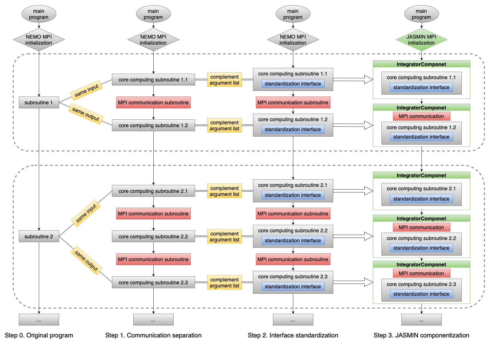
In NEMO, the time integration process is divided into subroutines distributed in various FORTRAN modules. In order to match the “communicate–compute” scheme of JASMIN components, subroutines with several communication calls need to be further segmented. Furthermore, the variables which are used by the subroutines and reside in global spaces in NEMO, need to be provided through the component interfaces from JASMIN patches. Therefore, in order to ensure correctness, we adopt a bottom-up strategy for the code refactorization process, including three steps: (1) the separation of communication, (2) the standardization of call interfaces, and (3) the formulation of JASMIN components. The whole process is shown in Fig. 2, with each step detailed in Sect. 2.1.1 through 2.1.3. In total, during the refactorization, we have formulated 155 components (i.e., FORTRAN subroutines) and 422 patches (i.e., model variables) in OMARE.

Figure 2 Overview of code refactoring process.

2.1.1 Communication separation

We separate the MPI communication in NEMO (e.g., lbc_lnk and mpp_sum) from subroutines and divide each subroutine into smaller ones which only contain computational codes. As in Fig. 2, each step of the time integration of NEMO consists of a series calls to FORTRAN subroutines (step 0). For the first step of separating the communication, we segment the core computing subroutines from the calls for boundary exchanges. In Fig. 2, subroutine 1 shares the same input as the core computing subroutine 1.1 and the same output as the core computing subroutine 1.2, with communication in between. Using the subroutine dyn_adv as an example, we first expose the “select-case” structure in the time-stepping program for the direct control of the parameterization schemes. Notice that there is a required boundary exchange (lbc_lnk) within the subroutine dyn_keg, and we separate it and split dyn_keg into two core computing subroutines: dyn_keg1 and dyn_keg2. For comparison, since the subroutine dyn_zad does not contain communication, it consists of a single computing subroutine. Consequently, for dyn_adv we finish the communication separation and get three core computing subroutines (step 1 of Listing 1).

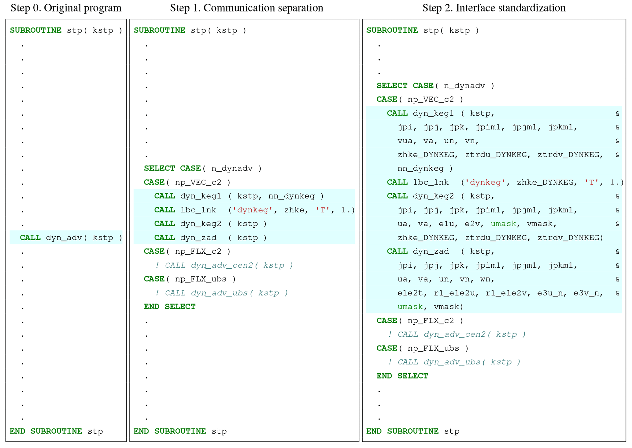
Listing 1 Code example of subroutine dyn_adv from communication separation to interface standardization. The highlighted areas are the actually executed code in the porting example.

2.1.2 Standardization of interfaces

NEMO manages all variables in the public workspace in various modules, so that every subroutine can directly access these variables without the need of passing them as parameters. This simplifies the coding process but compromises the “statelessness” of the code. Here, we complement the argument list of every core computing subroutine with a standardized interface (step 2 of Fig. 2). The standardized interface contains all variables the subroutine needs and divides these arguments into four categories: time, index, field, and scalar. This process makes the subroutine “stateless”. The time refers to the time step (a.k.a. kt in NEMO). The index refers to the generic size information of domain decomposition, such as jpi, jpj, and jpk. The field refers to field variables, such as prognostic variables, diagnostic variables, and additional scratch-type variables. They correspond to the data held by JASMIN patches. The scalar refers to parameters of the process control in the subroutine. All these arguments are declared and defined in the standardized version the subroutine. 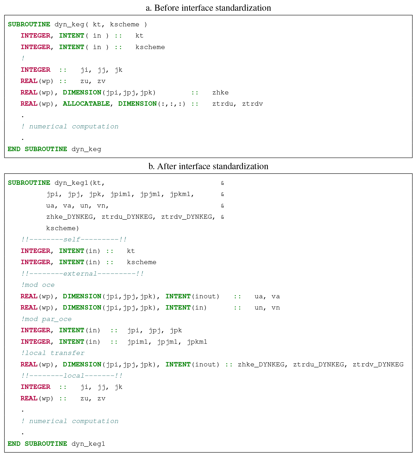As an example, for core computing subroutine dyn_keg1, the original subroutine dyn_keg only contains the time step argument kt and a scalar argument kscheme (Listing 2a). After complementing the argument list during the standardization of the interface (Listing 2b), the arguments are organized into four categories. Besides kt and kscheme, the index parameters jpi, jpj, jpk, jpim1, jpjm1, and jpkm1 and field variables ua, va, un, and vn, which are from NEMO's OCE module, are included. One thing to note is we change three local variables to the public space of the module dynkeg and rename them using the suffix of the module name, in case that they need to be transferred between the split subroutines. In the front of subroutine dyn_keg1, we declare the data type, size, and intent type of each argument and arrange them according to their source modules. Taking the same way to reconstruct subroutine dyn_keg2 and dyn_zad, we can finally refactor the subroutine dyn_adv from step 1 to step 2 in Listing 1. After the standardization of interfaces, the whole code base is still based on NEMO. There is no change in the simulation result, which is used for the correctness check of the refactorization process.

Listing 2 Code example of subroutine dyn_keg1 for the interface standardization.

2.1.3 Formation of JASMIN components

Next we change the whole NEMO environment to JASMIN. The control of the MPI is to be transferred from NEMO to JASMIN, including the initialization of MPI environment, domain decomposition, process mapping, and communication. In addition, all NEMO variables need to be replaced by the patch data, which are both initialized and provided by JASMIN.

For each subroutine with the standardized interface, we provide a JASMIN wrapper, which is a derived C++ class of JASMIN component. For the exemplary subroutine dyn_keg2 with standardized interface, the component DynKeg2PatchStrategy is constructed using JASMIN nomenclature (Listing 3). Furthermore, two functions are implemented (i.e., instantiated virtual functions in C++). Firstly, the function initializeComponent serves as the necessary boundary exchange for the patch data zhke_DYNKEG, which corresponds to the FORTRAN subroutine lbc_lnk in NEMO. The argument “NEMO_BL_INTERP” is a user-defined spatial interpolator during refinement, and it will be further discussed in Section 2.2. Secondly, we implement the function computeOnPatch which is a wrapper to the FORTRAN subroutine dyn_keg2. On the technical side, it is actually renamed as __dynkeg_MOD_dyn_keg2 after name mangling through FORTRAN/C++ hybrid compilation. Furthermore, we need to get patch data from JASMIN workspace and add JASMIN-provided variables to the subroutine's interface, so that to complete the argument list. This component patch strategy will be called by a corresponding numerical integrator component DynKeg2_intc and thus can be called by the time step in JASMIN (step 3 of Fig. 2).

Listing 3 Code example of subroutine dyn_adv in JASMIN time-stepping arrangement after componentization.

Listing 4 shows the porting result of the whole subroutine dyn_adv which is already in C++. The time-stepping function advanceLevel serves to do the integration in JASMIN like the subroutine stp in NEMO. The JASMIN (or OMARE) version of subroutine dyn_adv, which is part of stp, is composed of three numerical integrator components: DynKeg1_intc, DynKeg2_intc and DynZad_intc. The actual operations of these components are carried out by calls to the function of computing. Three variables are transferred: level refers to the current level of the grid hierarchy (i.e., resolution), current_time refers to the current time step, predict_dt refers to the time step in the current level. The switch-case structure in C++ is consistent with the logic of the original FORTRAN code in NEMO. The function calls to the other two parameterization schemes are put in place for future porting.

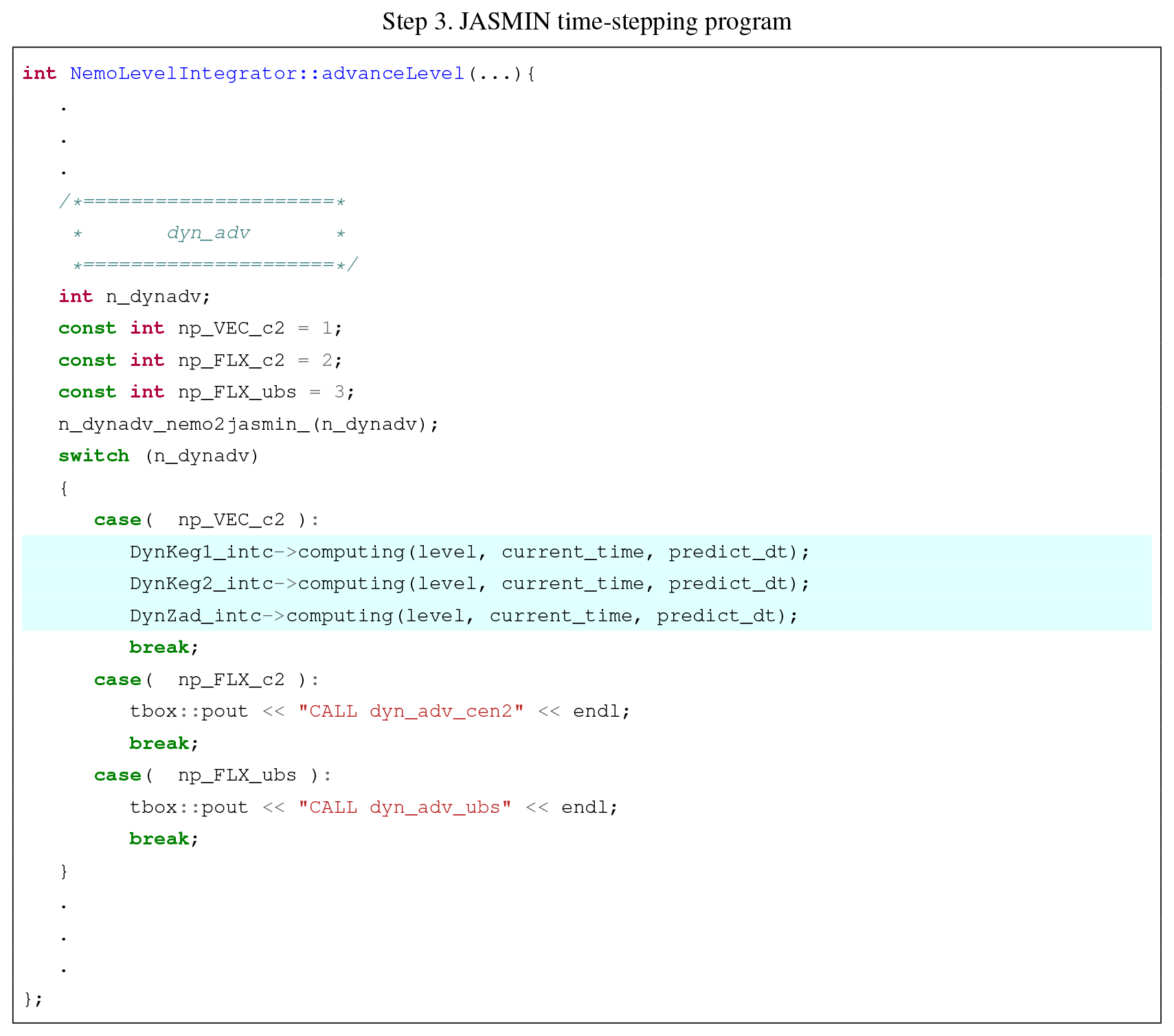
Listing 4 Code example of subroutine dyn_adv in JASMIN time-stepping program after formulating the components. The highlighted areas are the actually executed code in the porting example.

Following this manner, we refactor the whole time integration of NEMO onto JASMIN (step 3 of Fig. 2). Under the JASMIN context, the integrator component frees users from parallel programming and further supports AMR. For model diagnostics that rely on global reductions, we utilize JASMIN's reduction integrator components. For model initialization, we also design dedicated initialization integrator components, which manage all field variables through JASMIN patches. The allocation, deallocation, and communications are then carried out and further managed by JASMIN. Since the patches are all managed by JASMIN, including their distribution on processors, the operations required for AMR are enabled by JASMIN, including the change of refinement settings, patch generation, and domain decomposition into patches. With the provided OMARE code base, one can browse and build the code, and further run it with JASMIN (see Code Availability section for details). A short manual of installing JASMIN and building/running OMARE is provided in the Supplement.

2.2 Refinement in OMARE

OMARE utilizes the two-dimensional adaptive refinement functionalities of JASMIN. The spatial refinement is only carried out in the horizontal directions (similar to AGRIF-based NEMO), mainly due to the anisotropy between the horizontal and vertical directions of the ocean processes at large scales. Multi-level, recursive refinement is also supported, with the refinement ratio between the resolution levels specified by users in the OMARE's namelist. Accordingly, the temporal refinement is accompanied with spatial refinements, and it can be set independently from the spatial refinement ratio, in order to be flexible for improved efficiency and stability. Furthermore, in the current version of OMARE, we only consider one-way, coarse-to-fine forcings but not the interaction or feedback from the fine level. Related issues are discussed in Sect. 3 and further in Sect. 4. Details of the refinement in OMARE are introduced below.

2.2.1 Time integration

To support adaptive refinement in OMARE, we introduce super cycles in the time integration. Each super cycle consists of a fixed number of baroclinic steps at the coarsest resolution of the grid hierarchy. At the beginning of each super cycle, the grid refinement setting can be adjusted by specifying a refinement map (also a patch in JASMIN). The refinement map contains the Boolean flags marking each grid point as to whether it will be refined to the next level of resolution. User-specified refinement criteria can be integrated in OMARE, including adaptivity to temporally changing features (details in Sect. 3.4). The time step for the super cycle (i.e., baroclinic step count) can also be specified in the namelist of OMARE.

Figure 3 shows the overall time integration in OMARE. After the refinement map is set at the beginning of the super cycle, the grid hierarchy will be (re)constructed if the map is changed. The construction consists of the domain decomposition, the mapping to the MPI processes, and the construction of the communication framework, as well as necessary operations on the model status. First, the migration of model status is needed in the case of a new domain decomposition. The second case is to create a fine-resolution model status from that on a coarse grid, for newly refined regions. The level hierarchy is a data structure that manages all levels of the JASMIN framework, including the level number and the refined ratio. In OMARE, currently we initialize the model's prognostic status on each newly created fine-resolution grid point with surrounding coarse-resolution grid points through (bi)linear interpolations.

For each baroclinic step (on the coarse level), the time integration is carried out recursively on all levels throughout the grid hierarchy. The temporal refinement ratio controls the baroclinic step count on the finer levels. On the finer level, the time integration is carried out after the integration on the coarser level is finished (i.e., time step k+1 in Fig. 4). Accordingly, on the lateral boundaries between the coarse and fine levels, the model status on the coarse level provides these conditions at each fine-level time step (between k and k+1 step on the coarse level in Fig. 4). For OMARE, since we use the split-explicit formulation for barotropic and baroclinic processes, with each baroclinic step containing several barotropic steps, the model status for the barotropic and baroclinic steps is kept on the coarse level grid for spatial and temporal interpolations for the fine level.

2.2.2 Inter-level interpolations

In order to force the fine level with the outer, coarse level, an inter-level halo region is automatically created for the fine level by JASMIN. The halo region has the same resolution as the fine level, but the model status is specified on the fly with the coarse-level model status. The width of the halo region can be specified through OMARE's namelist. Figure 4 shows a sample case involving two resolution levels, with (1) a (spatial) refinement ratio of 3 and (2) a halo width of 1. In particular, the refined region has a irregular shape (i.e., non-square), and the inter-level halo is created accordingly (marked in yellow). The physical boundary of the case, marked in grey, does not participate in the inter-level halo but constrains the model status on both the coarse and the fine level through the physical boundary conditions.

For the spatial and temporal interpolation of the model status on the inter-level halo, we currently implement a basic set of linear interpolations in OMARE. For temporal interpolation, we adopt intrinsic interpolators built in JASMIN, which is standard linear interpolation. This applies to both barotropic and baroclinic model status as provided on the coarse level. For spatial interpolations, we implement variable-specific (bi)linear interpolators. Specifically, we implement three interpolators, NEMO_BL_INTERP, NEMO_U_INTERP, and NEMO_V_INTERP, which are designed for non-staggered variables, variables on the east edge (i.e., u for Arakawa-C grid), and variables on the north edge (i.e., v). As shown in Fig. 4, the data on non-staggered locations of the target fine-level cell R are attained by interpolating the data of four surrounding coarse-level cells (C₁ to C₄), which are implemented in NEMO_BL_INTERP. For u points, the interpolation involves two or four adjacent cells. The data U_c1 to U_c4 on the coarse t point C₁ to C₄ correspond to the u point $C_{\mathrm{1}}^{\prime }$ to $C_{\mathrm{4}}^{\prime }$ (from the dashed vector to the solid vector in Fig. 4), with an example target location at R^′. This interpolator is implemented as NEMO_U_INTERP. Similar treatment to points on v points in Arakawa-C grid is carried out accordingly, which corresponds to NEMO_V_INTERP. For the fine cells near the physical boundary, we have the following specific treatments. In the case that no valid data are available for interpolation, the bilinear interpolation degenerates to the linear or the nearest-neighbor interpolation. For model status on physical boundaries, we override the interpolated values according to proper boundary conditions if necessary.

In general, the overall routines of inter-level interpolation are similar to AGRIF-based NEMO, with the key difference in OMARE being that irregular refinement regions, as well as adaptive refinement, are enabled in OMARE. User-specified interpolators, including NEMO_BL_INTERP, NEMO_U_INTERP, and NEMO_V_INTERP, are examples of bespoke interpolation functions that are possible in JASMIN. More sophisticated interpolators (i.e., conserved ones for fluxes, high-order algorithms, as in Debreu et al., 2012, and AGRIF-based NEMO) are planned for the future development of OMARE.

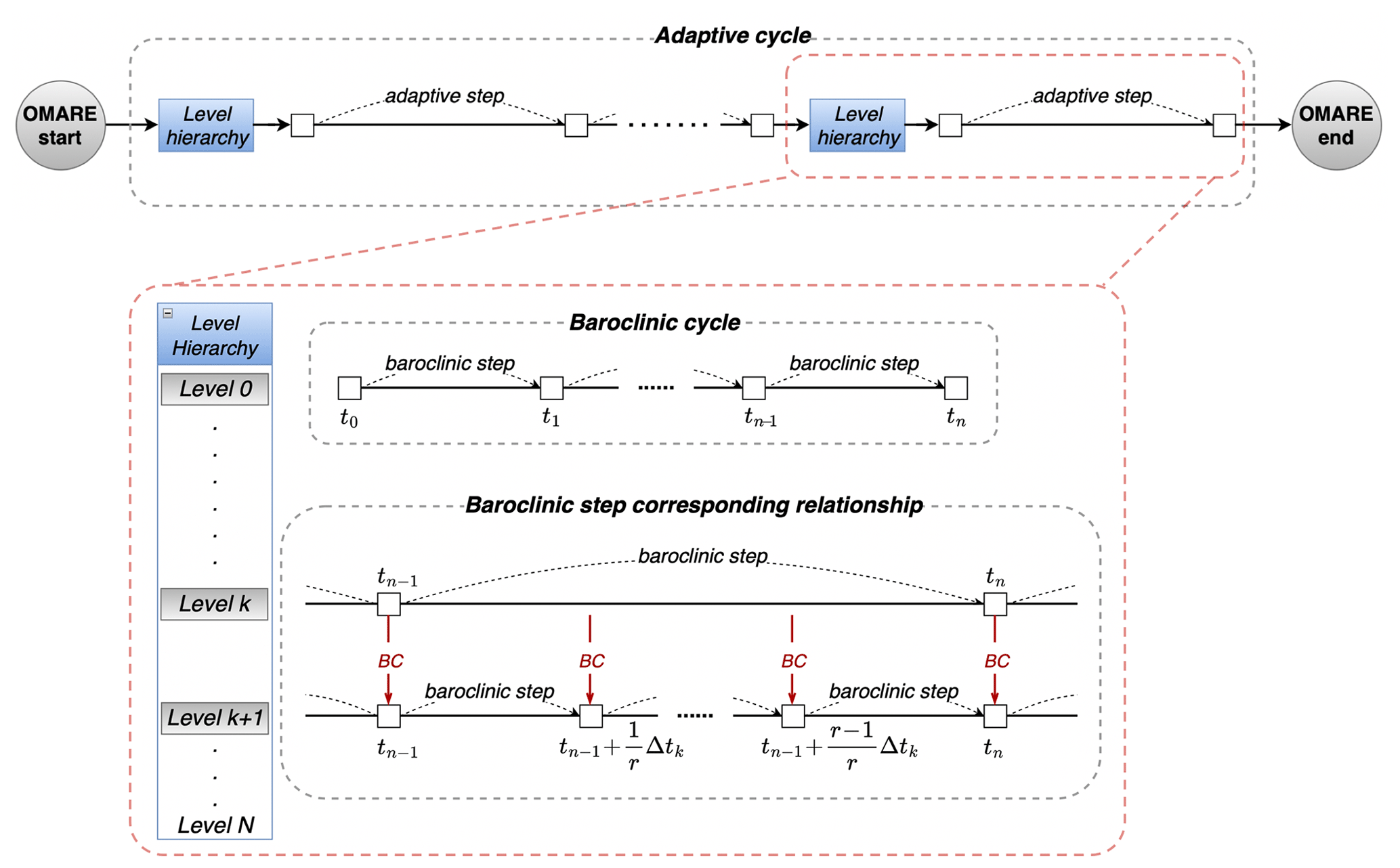
Figure 3 Flow chart of the time stepping in OMARE. The whole integration consists of many super cycles, with each super cycle consisting of several baroclinic steps on the coarsest resolution level. The grid and resolution hierarchy is (re)constructed at the beginning of an adaptive step according to the user-defined refinement criteria. The relationship between two adjacent resolution levels, k and k+1, in the level hierarchy is shown in detail (dashed red box). The temporal refinement ratio from level k to level k+1 is r. A single baroclinic step (from t_n−1 to t_n) of level k corresponds to r baroclinic steps of level k+1. The time steps on the two levels are Δt_k and $\frac{\mathrm{1}}{r}\mathrm{\Delta }{t}_k$, respectively. The lateral boundary conditions (BCs) are provided through online interpolations between adjacent levels.

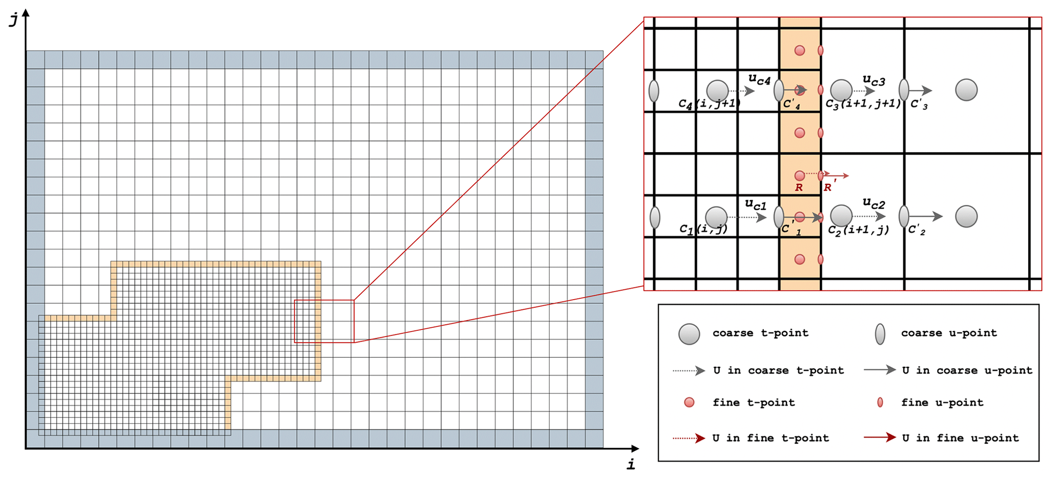
Figure 4 Example of a refinement region with an irregular boundary (refinement ratio 1:3) with the idealized test case in Sect. 3. The size of the coarse grid for the modeled ocean basin is 30×20. Physical boundaries are marked by grey cells. The inter-level halo, marked by yellow cells, is controlled by the coarse level but on the same resolution as the fine level. A specific region on the coarse level-fine level boundary is shown on the right, with details of the variable layout (u and t).

3 Model settings and numerical experiments

3.1 Typical resolutions and model configurations

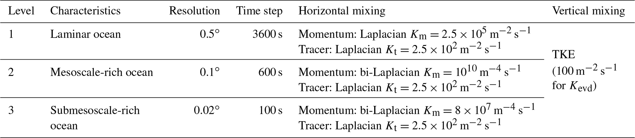
In OMARE we focus on three typical spatial resolutions, as shown in Table 1. While 0.5^∘ resolution (or coarser) is mainly used for climate models and long-term time integration, the model cannot simulate the ocean's mesoscale process and the geostrophic turbulence. We denote the ocean as simulated by the 0.5^∘ model as the laminar ocean. The second resolution of 0.1^∘ is 5 times finer than the first resolution of 0.5^∘ and is commonly used in the community for eddy-/mesoscale-rich simulations. The nominal 10 km grid spacing is capable of resolving the first baroclinic Rossby radius of deformation in midlatitudes, which is about 50 km at 30^∘ N (Chelton et al., 1998). The finest resolution is 0.02^∘ and another 5 times finer that 0.1^∘. This resolution corresponds to about 2 km grid spacing in the midlatitudes, and it is usually adopted for submesoscale-rich simulations (Rocha et al., 2016). These resolutions form the three-level resolution hierarchy in OMARE .

Furthermore, we adopt the following model configurations for each specific resolution. The baroclinic time steps of the three resolutions are chosen as 1 h for 0.5^∘, 600 s for 0.1^∘ (or $\mathrm{1}/\mathrm{6}$ that of 0.5^∘), and 120 s for 0.02^∘ (or $\mathrm{1}/\mathrm{5}$ that of 0.1^∘), respectively. The purposeful decrease ratio in the time step at 0.1^∘ of $\mathrm{1}/\mathrm{6}$ (instead of the 1:5 resolution difference) is to ensure better numerical stability at finer resolutions. The barotropic time step is computed proportionally according to the baroclinic time step size, in order to accommodate the nominal surface gravity wave speed. For the vertical coordinate, OMARE uses the same z coordinate, with the same vertical layers across the three horizontal resolutions. The (adaptive) grid refinement is only carried out in the horizontal direction. For the vertical coordinate, we adopt the following scheme for all numerical experiments: the layer depth starts at 8 m in the mixed layer and gradually increases to over 150 m towards the ocean abyss. For the maximum depth of 4200 m, there are 50 vertical layers in total.

For the horizontal mixing parameterization, we adopt different schemes for the three resolutions. For the momentum mixing, at 0.5^∘ we adopt the first-order Laplacian isotropic viscosity, and at 0.1 and 0.02^∘, we adopt second-order, bi-Laplacian viscosity. For tracer mixing, we simply apply a uniform diffusivity parameter across the resolutions (Table 1). For the vertical mixing parameterization, we adopt the same turbulent closure parameterization scheme (turbulent kinetic energy, TKE) across the three resolutions, with enhanced mixing for very weak stratification. The choice of parameters is preliminary and is subject to further tuning in the future.

The choice of parameterization schemes and parameters is comparable with studies with similar resolution settings (Schwarzkopf et al., 2019).

Table 1 Model configurations of the resolution hierarchy of three levels.

3.2 Double-gyre test case

In this study we use an idealized double-gyre test case to test OMARE with the mesoscale and submesoscale processes on the western-boundary current (WBC) system. The modeled region is a rectangular, closed ocean basin on the β plane, centered at 30^∘ N. The size of the ocean basin is 3000 km in the zonal direction and 2000 km in the meridional direction. The depth of the ocean basin is uniformly 4200 m (or 50 layers). The free-slip lateral boundary condition is used for all the experiments and across all three resolutions.

The atmospheric forcing is a normal year, seasonally changing forcing with both dynamic and thermodynamic components. Each model year consists of 360 d, divided into 12 months, with 30 d per month. The wind stress is purely zonal (i.e., only U wind stress) and a distinct seasonal cycle of both wind strength and wind direction turnaround latitude. The thermodynamic atmospheric forcing is carried out using a temperature-based recovery condition for the ocean surface. The forcing is introduced in detail in Appendix A, with Fig. 5 showing the extreme conditions in summer and winter.

The model is initialized to a stationary state with uniform vertical profiles for temperature and salinity across the basin. The mean surface kinetic energy reaches a quasi-equilibrium status after 20 years from the start, and the system forms the subtropical gyre, the subpolar gyre, and the WBC system. Figure 5c shows the annual mean sea-surface height (SSH) after 50 years with 0.5^∘ resolution.

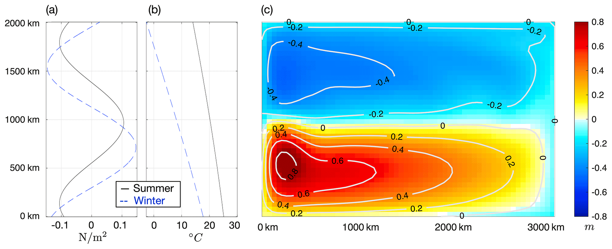
Figure 5 Zonal wind stress (a), sea-surface temperature (b), and the sea-surface height climatology under 0.5^∘ resolution (c).

3.3 From laminar ocean to mesoscale-rich, turbulent ocean

Based on a 50-year spin-up run with 0.5^∘ resolution, we carry out three experiments with 0.1^∘ resolution. We denote the experiment with 0.5^∘ resolution as “L”, standing for “laminar ocean”. A full-field 0.1^∘ experiment (denoted “M”) is carried out through the online refinement based on the 0.5^∘ experiment by mapping of the model's prognostic status at 00:00 on 1 January in model year 51. Furthermore, two parallel 0.5–0.1^∘ experiments with different regional refinement to 0.1^∘ are carried out, as shown in Fig. 6. Since these two experiments involve two interactive resolutions, we denote them as L-M-I and L-M-II, respectively. The region of 0.1^∘ resolution is interconnected and has irregular boundaries, covering the western boundary, the majority of the northern and southern boundary, WBC, and the extension of the WBC. In addition, in the subpolar gyre, the refined region to 0.1^∘ in L-M-I covers more area than that in L-M-II. Conversely, in the subtropical gyre, the refined region is smaller in L-M-I than that in L-M-II. The area of the region refined to 0.1^∘ is 56 % and 61 % of the whole basin for L-M-I and L-M-II, respectively.

Compared with 0.5^∘ resolution, the experiment with 0.1^∘ resolution shows much higher overall kinetic energy (Fig. 7). At equilibrium, the annual mean surface KE is about 0.035 m⁻² s⁻² for 0.1^∘, which is about 2.5 times that at 0.5^∘. This corresponds to the mesoscale turbulence, which manifests at the spatial resolution of 0.1^∘ (10 km) or finer. For comparison, at 0.5^∘, the model only simulates laminar flow, despite the presence of WBC (Fig. 5b and video supplement). Also the distinct seasonal cycle of surface KE at 0.1^∘ is both larger in magnitude (0.01 m⁻² s⁻² v.s. 0.005 m⁻² s⁻²) and different in terms of the month with maximum KE (May vs. March).

Interestingly, there is a sudden jump of KE (from 0.015 to 0.07 m⁻² s⁻²) within the first 3 months of the resolution change to full-field 0.1^∘. The excessively high KE gradually decreases towards the end of year 53 (i.e., 3 years after the change in the resolution). Further examination of the SSH field at equilibrium status for 0.1^∘ experiment reveals systematically lower mean potential energy (PE) than the 0.5^∘ experiment (Fig. 8, first row). Both the subtropical gyre and the subpolar gyre show lower absolute values of SSH for 0.1^∘ experiments (Fig. 8b). Correspondingly, while the SSH difference between the two gyre centers is over 1.2 m for 0.5^∘ experiment, that for 0.1^∘ experiment is only about 70 cm. This result indicates that there is higher mean PE in the 0.5^∘ experiment that cannot be sustained in the 0.1^∘ experiment. The mean PE is released after the change of resolution to 0.1^∘, causing the high KE during the first 2 years after resolution change. The overall difference in the kinetic energy and the mean PE, as well as the transitional phase, imply the drastically different energy cycles at the two resolutions. While 0.5^∘ or similar resolutions are adopted in climate models, it cannot accurately characterize the conversion of energy from the atmospheric kinematic input and the ensuing energy transfer and cascading.

Furthermore, the two regional refinement experiments (L-M-I and L-M-II) reveal further evidence of the energy cycles. Similar to the full-field 0.1^∘ experiment, they both show (1) a high KE during the first 2 years (i.e., a spin-up process) after refinement and (2) a gradual adjustment to equilibrium KE which is attained after 5 years. However, although they both have a partial region of the basin with 0.1^∘ (56 % and 61 % respectively), they show higher KE than the full-field 0.1^∘ experiment. In particular, for L-M-I, the mean surface KE is at 0.054 m⁻² s⁻² (year 56 to 60) which is about 50 % higher than M. For L-M-II, the mean surface KE is marginally higher than M by 14 %, at 0.04 m⁻² s⁻².

The systematically higher KE is mainly due to the lateral forcing of the model status at 0.5^∘ on the refined, 0.1^∘ regions through the boundary (Fig. 8). In both L-M-I and L-M-II, the region of 0.1^∘ contains the WBC, the western boundary of the basin, and the majority of the northern and southern boundary. The full-field 0.5^∘ simulation, which is carried out online with the 0.1^∘ simulation, casts influence on the 0.1^∘ region through the boundary, affecting all the model's prognostic status including barotropic speed, baroclinic speed, surface height, temperature, and salinity. The effect of the systematically high SSH in 0.5^∘ region is most evident on the zonal 0.5–0.1^∘ boundary in the subtropical gyre in L-M-I. There is a local SSH maximum (indicated by 0.6 m SSH isobath), which is separated from the SSH core of the subtropical gyre to the west end of the basin. For comparison, in L-M-II, the region with 0.1^∘ in the subtropical gyre extends further to the east by 800 km. As a result, the SSH in the subtropical gyre, including both the SSH on the 0.5–0.1^∘ boundary and the overall SSH of the gyre, is reduced and more consistent with the full-field 0.1^∘ experiment (M).

The modeled SSH and the surface KE also show higher sensitivity to the refinement in the subtropical gyre than in the subpolar gyre. Comparing L-M-I and L-M-II, we show that with increased (reduced) zonal coverage of the refined region for both subtropical and subpolar gyre, the mean SSH in the gyre becomes closer to that in M. However, when a greater portion of the subtropical gyre (other than the subpolar gyre) is included for refinement, both SSH and KE show a higher degree of consistency with the full-field 0.1^∘ experiment. This is potentially related to the higher absolute SSH in the subtropical gyre than the subpolar gyre, which is consistent across both 0.5 and 0.1^∘ experiments. With higher SSH in the subtropical gyre as simulated with 0.5^∘, the boundary between 0.5 and 0.1^∘ enforces higher SSH in the 0.1^∘ region, with more ensuing PE–KE conversion and higher KE (Fig. 7). In summary, we find that the difference in the sensitivity of the mean KE to refinement settings is the result of both the climatological SSH and the specific choices of refinement regions. Although eddy-rich ocean simulations are becoming more available to the community, climate simulations still rely heavily on 0.5^∘ or even coarser resolutions (Tsujino et al., 2020). The resolution hierarchy of 0.5, 0.1, and 0.5–0.1^∘ refinements in OMARE serves as a basic framework for the further study of the oceanic energy cycle of numerically laminar and turbulent oceans.

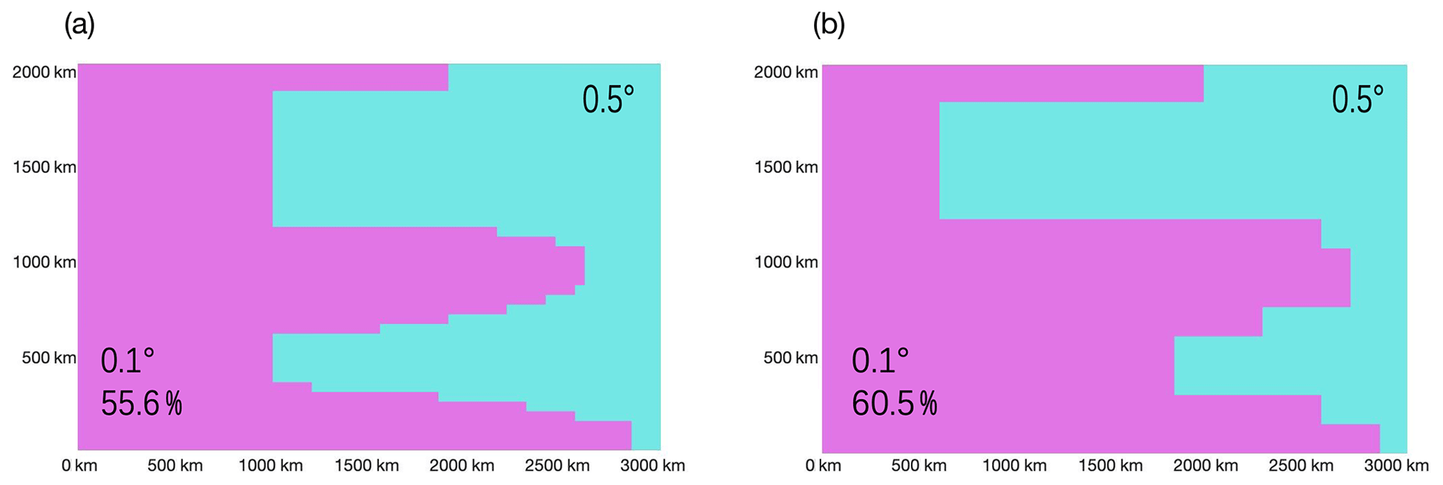
Figure 6 Two regional refinement settings from 0.5 to 0.1^∘ of the double-gyre case. Panels (a) and (b) show L-M-I and L-M-II respectively. The background and the whole ocean basin are, by default, in 0.5^∘ resolution and marked in cyan, and the region refined to 0.1^∘ in each experiment is marked in purple.

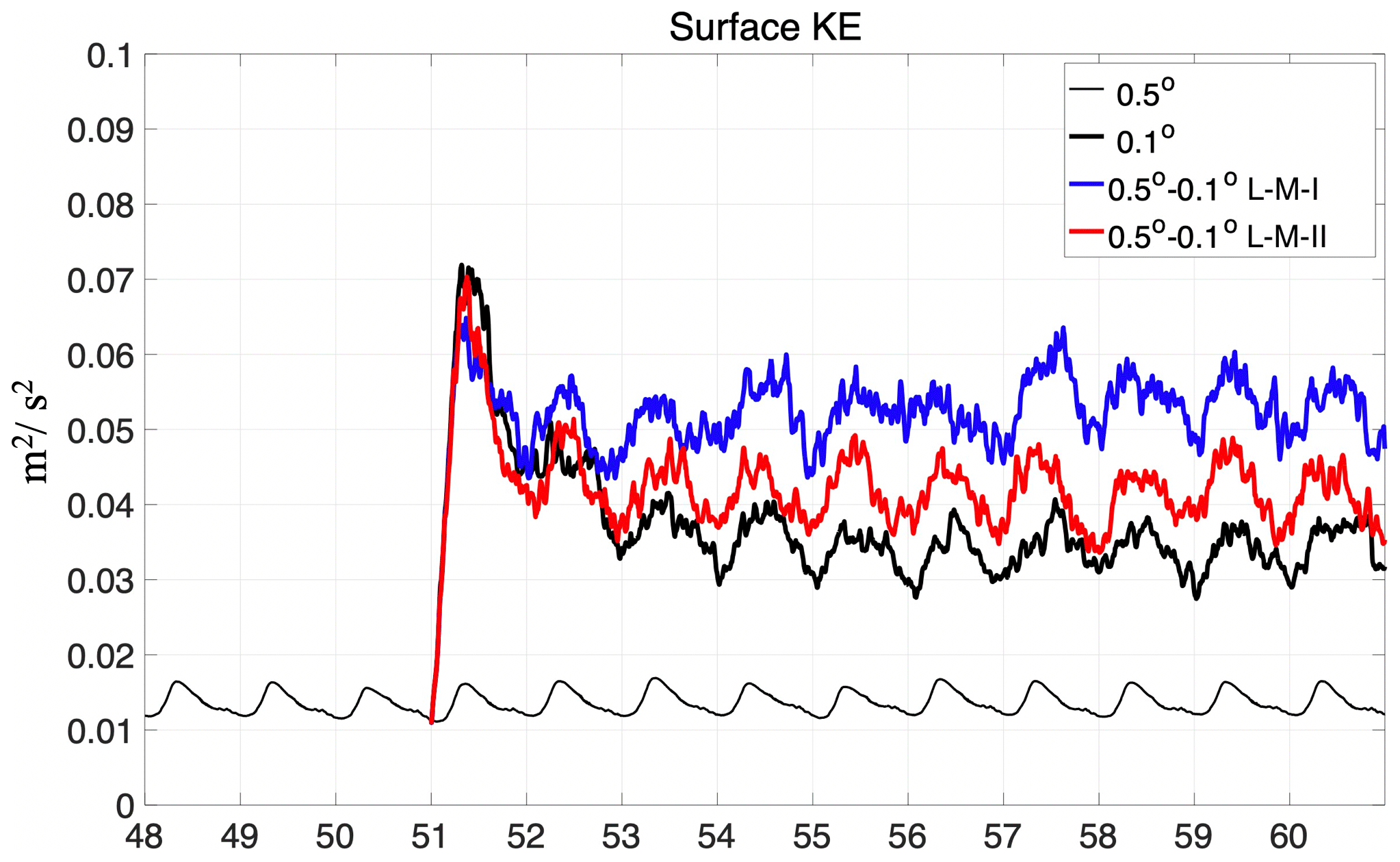
Figure 7 Mean surface kinetic energy of experiments with full-field 0.5^∘ (L, thin black line), a spin-off full-field 0.1^∘ (M, thick black line) since year 51, and two spin-off 0.5–0.1^∘ regional refinement experiments (L-M-I and L-M-II, in blue and red lines, respectively).

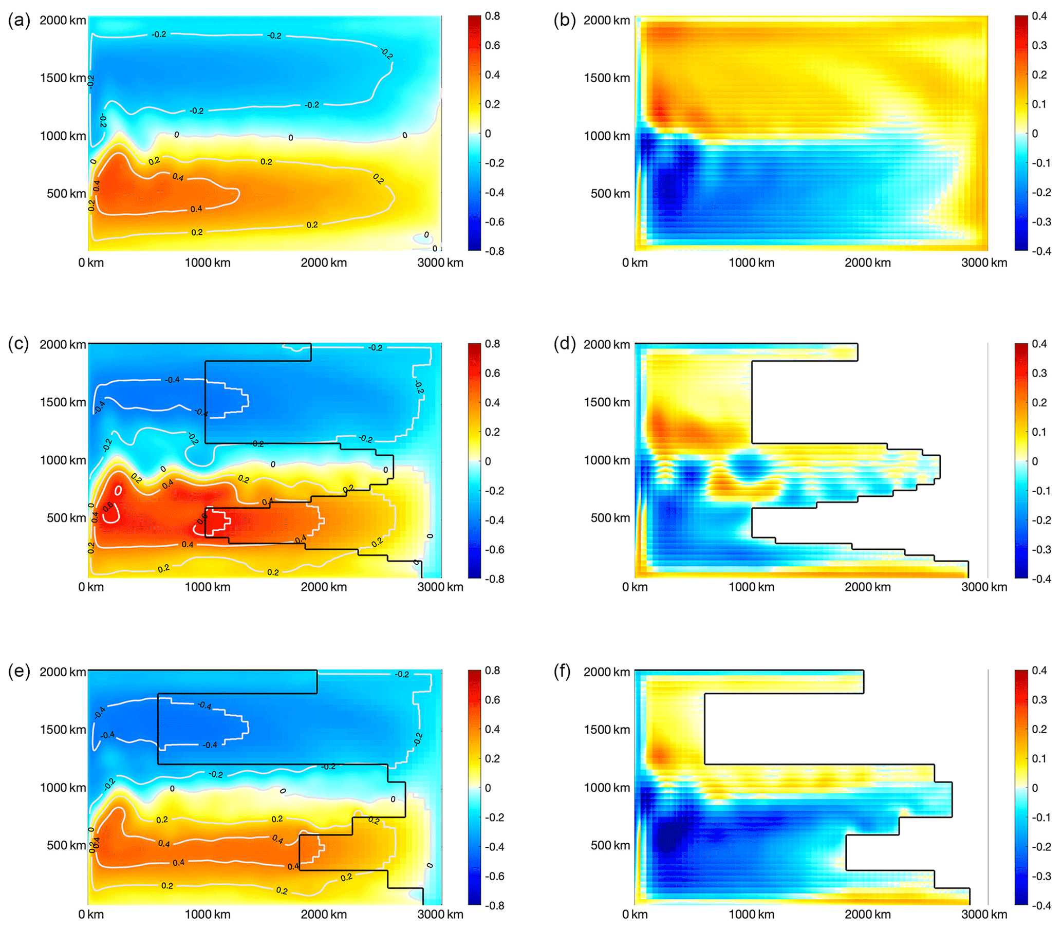
Figure 8 SSH climatology (a, c, e) of the full-field M experiment (a, b) and two regionally refined 0.5–0.1^∘ experiments (L-M-I and L-M-II in c, d and e, f). Difference with 0.5^∘ simulations is shown in (b), (d), and (f), respectively.

3.4 Adaptive refinement to 0.02^∘ and submesoscale processes on WBC

Based on the full-field 0.1^∘ experiment, we further carry out the refinement to 0.02^∘ and focus on submesoscale processes on the WBC. Specifically, we adopt adaptive refinements in order to capture temporally varying mesoscale and submesoscale features, using surface velocity and relative vorticity as indicating parameters. The model dynamically determines the region of refinement to 0.02^∘ based on the instantaneous model status, as well as the threshold values as listed in Table 2. If the absolute value at each grid cell is larger than the threshold, the cell is marked for refinement. The adaptive refinement is achieved by recomputing the region of refinement at a fixed interval (i.e., the super cycle of 5 model days).

It is worth noting that both the threshold values and the instantaneous fields are computed through spatial scaling. For example, in order to determine the threshold values, we accumulate 5-years' instantaneous fields of the 0.1^∘ experiment and compute the probability density of all the fields after spatial coarsening to 5×5 model grid cells (or 50 km×50 km). The spatial scaling algorithms are presented in Appendix B. Then, we choose the 80th and 90th percentile for the absolute velocity and the absolute value of the relative vorticity as the threshold values (Table 2). The reason that we use spatial coarsening is that the model's effective resolution is usually 5 to 10 times that of the grid's native resolution. By spatial coarsening of 5×5 grid cells on 0.1^∘ fields, we attain a more physically realistic representation of both speed and vorticity at the scale of 50 km (Rocha et al., 2016; Xu et al., 2021). Correspondingly, at each super cycle, we determine the instantaneous values of speed and vorticity at 50 km scale and compare against threshold values for refinement.

Similar to the 0.5–0.1^∘ experiments, we carry out three spin-off experiments from 0.1 to 0.02^∘ in both boreal winter and summer. With the full-field 0.1^∘ experiment, on 1 February and 1 August, we carry out a full-field 0.02^∘ experiment, as well as two adaptive refinement experiments, denoted M-S-I and M-S-II, respectively (Table 2). Figure 9 shows the mean surface KE of the three 0.02^∘ refinement experiments, up to 3 months after refinement. After full-field refinement to 0.02^∘, the model reaches the saturation of surface KE within 2 months. During winter (starting from 1 February), the model simulates continued KE increase even after 2 months (i.e., after April), which is due to the inherent KE seasonal cycle (the black line for 0.1^∘ as a reference). For the experiment during both winter and summer, the surface KE is about 60 % higher than the original 0.1^∘ experiment.

In contrast to 0.5–0.1^∘ experiments, the refinement to 0.02^∘ does not cause overshooting of KE (colored lines in Fig. 9). Furthermore, both AMR experiments show lower but also closer KE values to the full-field 0.02^∘ experiment (i.e., S) throughout each of the 3-month simulations. For refinement with 80th percentiles of surface vorticity and speed (i.e., M-S-I), the model attains over 90 % of the KE of the experiment S. The portion of refinement for M-S-I is temporally changing and is mostly lower than 50 %. For comparison, with 90th percentiles and M-S-II, the region of refinement is on average 30 % of the whole basin while attaining over 80 % of the total surface KE. The following part of the section examines the modeled submesoscale-scale processes at 0.02^∘ in detail.

Table 2 Threshold values of surface velocity and surface relative vorticity (both in magnitude) for adaptive refinement from 0.1 to 0.02^∘. Two settings are chosen, corresponding to the 80th and 90th percentile of the two parameters, based on the full-field 0.1^∘ experiment.

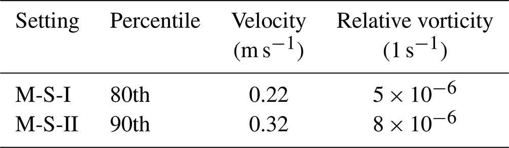
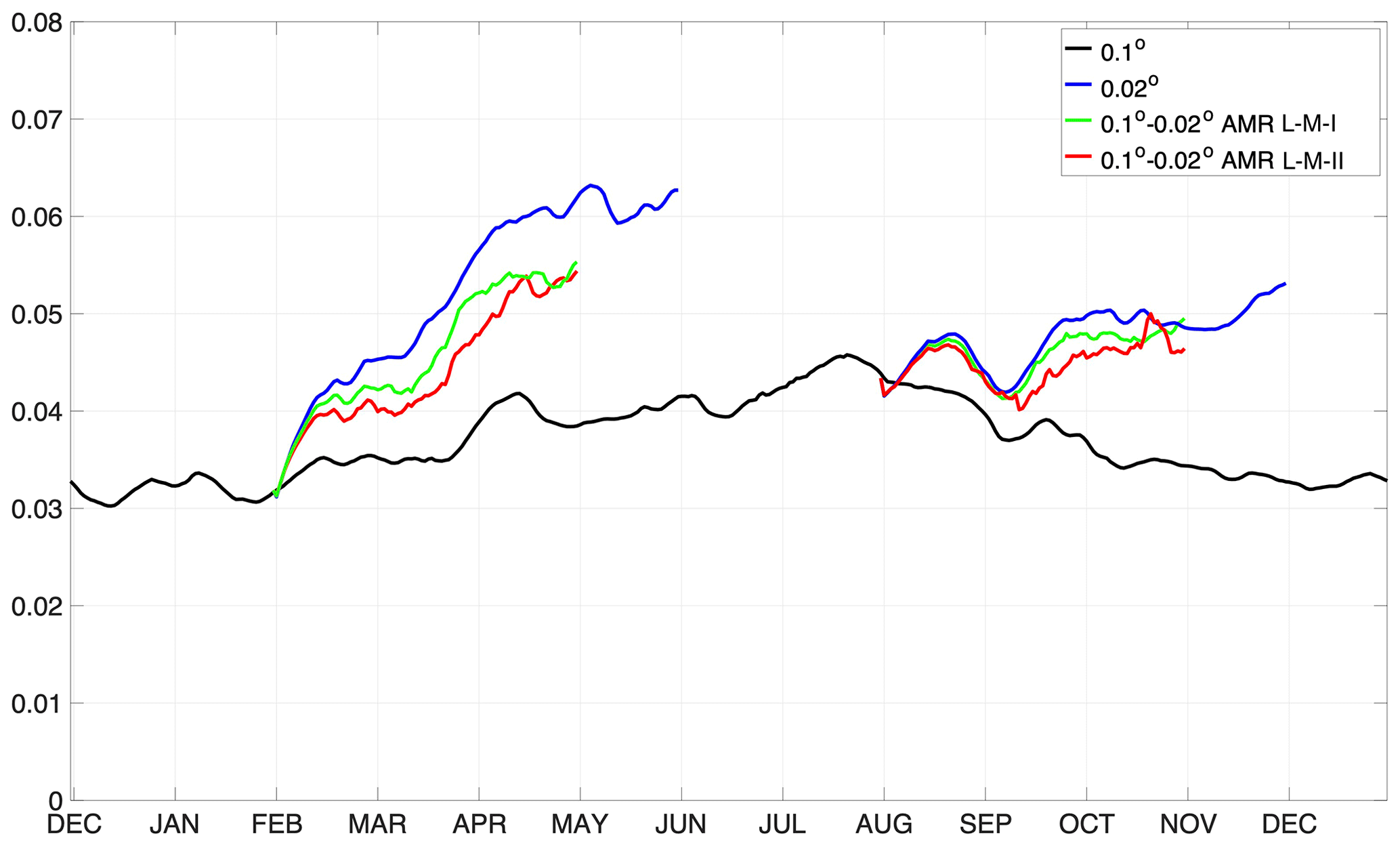
Figure 9 Surface mean kinetic energy (m⁻² s⁻²) in 0.02^∘ experiments and the associated 0.1^∘ experiment.

3.4.1 Submesoscale spin-up

During winter, the experiments with 0.02^∘ show prominent submesoscale development and associated features which are not captured by the 0.1^∘ experiment. In Fig. 10, we show the instantaneous surface Rossby number (or Ro, $\mathit{\zeta }/f$) fields after 5 d of refinement to 0.02^∘. Since adaptive refinement was based on the instantaneous field at 00:00 on 1 February, the model has carried out a 5 d time integration with the same refinement region. During these initial days after refinement, the mesoscale patterns across the three refinement experiments are very similar and consistent with the full-field 0.1^∘ experiment. The submesoscale processes are not fully developed in any of the 0.02^∘-related experiments, with regions with large values of Ro emerging from mesoscale features.

For M-S-II, the region of refinement during winter mainly consists of the southern boundary and the WBC (Fig. 10c). For the WBC, the region of refinement grasps the key features such as the mean flow, and the meandering WBC, as well as several strong mesoscale eddies. This indicates that with the threshold value-based criteria, the model is able to capture the region of focus, which is temporally changing mesoscale processes of WBC. The total area of refinement in Fig. 10c is about 30 %. Among all the grid cells, there are some cells that satisfy both refinement criteria for velocity and vorticity. Therefore, less than 20 % of cells should be marked for refinement. The actual refinement ratio is higher at 30 % and caused by two factors. First, the lateral boundaries are marked for refinement to 0.02^∘ by default (Appendix B). Second, there is automatic alignment of the refined region at 0.02^∘ to three cells at 0.1^∘ in each direction, in order to attain more regular patches at 0.02^∘. Both factors contribute to the larger ratio of refinement of about 30 %.

For M-S-I (panel b in Fig. 10), we use smaller threshold values, which result in larger refinement regions that extend to other parts of the basin, including (1) a greater portion along the southern boundary, (2) a larger portion on the WBC and its extension, and (3) other regions with intermittent high speed and/or vorticity, such as those in the northeastern part of the basin. In addition, the refined region on the WBC extends to the east and to either side of WBC and is very close and even linked to the refined region on the basin's southern boundary. Overall, the region of refinement is 46 % of the basin, which is larger than the maximum refinement ratio by the threshold values at 40 %.

Compared with the full-field 0.02^∘ experiment (panel a of Fig. 10), the major hot spots on the WBC and the boundaries are captured well by the two AMR experiments. The larger region of refinement in M-S-I than in M-S-II at 5 d is indicated in marginally higher surface KE in the former experiment (Fig. 9). Also, both experiments have smaller but close KE compared to the full-field 0.02^∘ experiment.

After another 15 d (or 20 d since 1 February), the overall mesoscale pattern witnesses gradual changes but remains consistent across all four experiments (Fig. 11). At this time, the model has undergone four full super cycles of refinement (i.e., each cycle of 5 d). In the AMR experiments, the major part of the WBC is always refined during the 20 d period, due to the constantly large magnitude of surface velocity and vorticity in this region (see also the corresponding video supplement). As a result, the submesoscale processes in WBC undergo continued development, and they show the same features as the full-field 0.02^∘ experiment. These features include the returning flow at (400, 800 km) and the large cyclonic eddy at (400, 500 km). In all three 0.02^∘ experiments, all the ocean fronts and filaments along the WBC and major submesoscale are more sharpened compared with 0.1^∘ counterpart. Certain areas with small-scale vorticity structures are modeled with full-field 0.02^∘ but not captured by AMR experiment, mainly due to these regions not being constantly refined throughout the 20 d's run. In terms of KE, both of the two AMR cases attain over 85 % of the total KE attained by full-field 0.02^∘ after 20 d of refinement (Fig. 9).

After 50 d of refinement, the submesoscale processes in 0.02^∘ regions in S, M-S-I, and M-S-II are well developed (Fig. 12). For full-field 0.02^∘, a large band rich in submesoscale features is present, with a continuum of small-scale vortices in the WBC extension and towards the east end of the basin. A certain part of this band, as well as the WBC, is captured in M-S-II (i.e., 80th percentiles). For comparison, in M-S-I, the major part of this band is not marked for refinement. It is worth noting that the refinement criteria are based on the field as simulated at 0.1^∘. During winter, the submesoscale processes and the ensuing kinetics are mainly driven by mixed layer instability (Khatri et al., 2021). At 0.1^∘ (or 10 km) resolution, the model cannot directly simulate these processes. Potentially, the refinement criteria can be augmented for these processes, if they are the subject of study with AMR.

We further examine the vertical motion on the fifth model layer (about 40 m depth) for all four experiments (Fig. S1). The most evident feature of all three 0.02^∘ experiments is the large vertical speed of nearly 100 m d⁻¹ that is prevalent mainly in the region associated with the WBC region. For comparison, the vertical velocity in the 0.1^∘ experiment is very muted, indicating that the submesoscale processes are not captured at this resolution. In the AMR experiments, these key regions with high vertical speed are captured well, with good reproduction of both the location of occurrence and its magnitude.

At 50 d, we are approaching predictability limitation for the ocean's mesoscale. Although the overall mesoscale pattern retains certain similarity across the experiments, noticeable differences emerge, especially between 0.02 and 0.1^∘. For example, the location of WBC branching off the west coast differs: at 500 km for 0.02^∘ experiments and at 700 km for the 0.1^∘ experiment. We further compare and analyze a typical transect in these experiment in the next section of the paper.

Also after 50 d, the difference between 0.02 and 0.1^∘ is more pronounced. Within the region of 0.02^∘, the model simulates stronger flow and sharper and finer structures overall. Since we do not include feedback of 0.02^∘ onto 0.1^∘ regions, in AMR experiments, the region with 0.02^∘ is actually forced by the full-field 0.1^∘ experiment through the lateral boundaries between 0.1 and 0.02^∘. The difference in model states at 50 d results in inconsistencies along the boundaries, including artificial convergence and gradients. Examples include the southern boundary of the WBC in Fig. 12. The “noises” on the resolution boundaries are not evident during the previous stages of refinement (i.e., Figs. 10 and 11, as well as video supplement), further indicating that they are caused by model state inconsistencies. We consider these noises are of numerical nature, and they can be reduced through interactions between the refined and the non-refined regions. We further discuss the future development of OMARE to support feedback of 0.02^∘ on 0.1^∘ in Sect. 4.

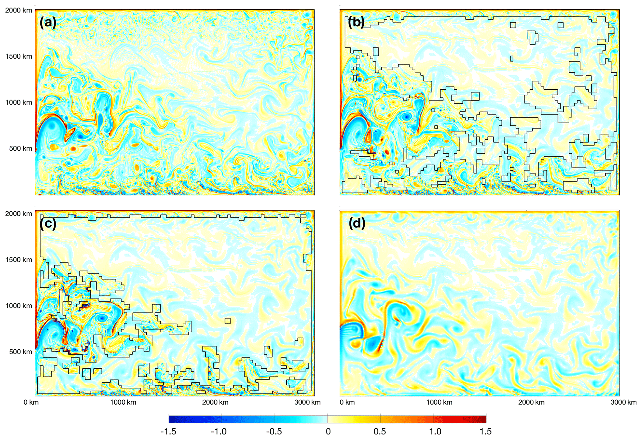
Submesoscale processes in the subtropics usually have pronounced seasonality. For comparison, in Fig. 13 we show the surface relative vorticity after 50 d of refinement during summer (i.e., since 1 August). In contrast to the winter, the surface KE in all refinement experiments is very close during summer (Fig. 9). The lower KE corresponds to the lower buoyancy input during summer, which greatly energizes the surface ocean during winter. Accordingly, the summertime vorticity field with 0.02^∘ is very muted, with the absence of small-scale, ageostrophic structures (Fig. 13a). In addition, the boundary-related numerical noise emerges as the AMR refinement experiments progress (see also the video supplement for earlier stages of refinement during summer).

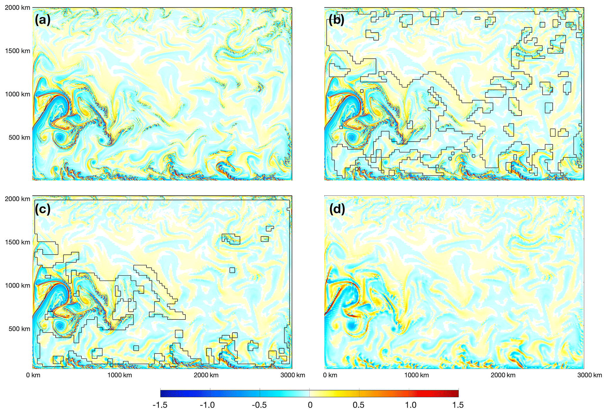
Figure 10 Surface Rossby number ($\mathit{\zeta }/f$) after 5 d of (adaptive) refinement from 0.1 to 0.02^∘ since 1 February. Panels (a), (b), and (c) shows the result for the full-field 0.02^∘ experiment (i.e., S), that of AMR setting 1 (i.e., M-S-I), and that of AMR setting 2 (i.e., M-S-II), respectively. In both AMR experiments (b, c), the boundary between 0.02 and 0.1^∘ is marked by black lines. Panel (d) shows the reference simulation result at 0.01^∘ on the same day.

Figure 11 Same as Fig. 10 but for 20 d after the refinement since 1 February.

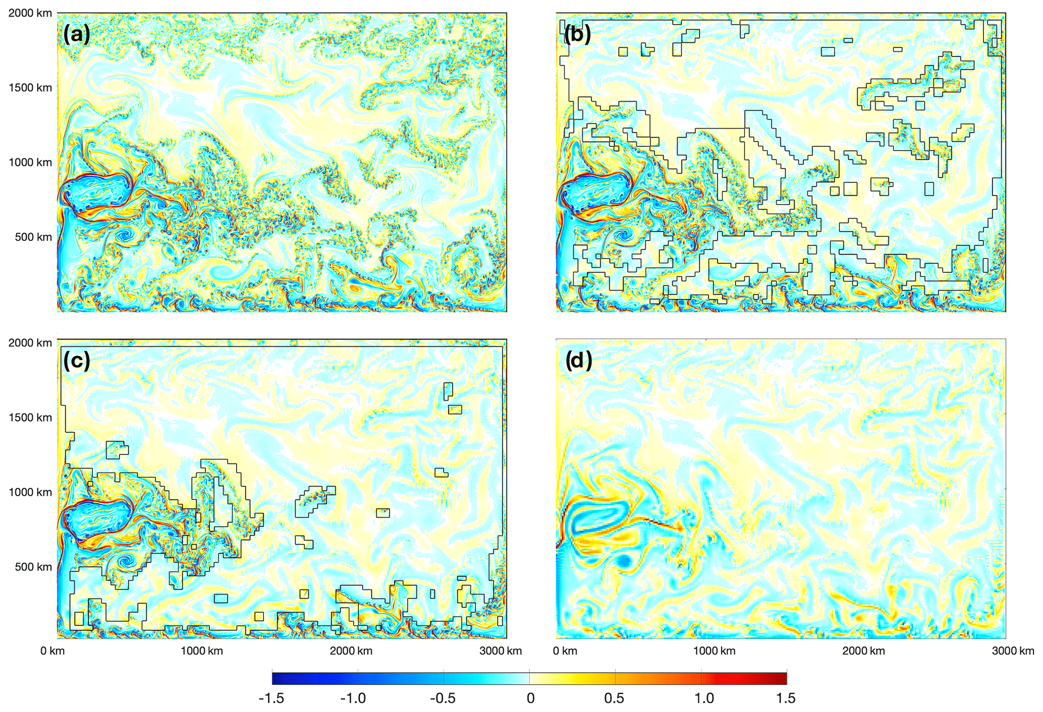
Figure 12 Same as Fig. 10 but for 50 d after the refinement since 1 February. In each panel, a meridional transect is marked by a dashed red line. In order to improve the consistency of mesoscale features along these transects, in panel (a), the location of the transect is 550 km from the western boundary, and in other panels, the location is offset to the east by 50 km, at 600 km.

Figure 13 Same as Fig. 10 but for 50 d after the refinement since 1 August.

3.4.2 Analysis of a typical transect

We further examine the mesoscale and submesoscale processes of the WBC in 0.02^∘ experiments. We pick a typical meridional–vertical transect for each experiment after 50 d of refinement to 0.02^∘. The transect is about 550 km from the west end of the basin for the full-field 0.02^∘ experiment (Fig. 12a). The transect traverses (1) the southern boundary; (2) the subtropical gyre, which includes large mesoscale features including a prominent coherent structure as an anticyclonic eddy (marked by I); (3) the eastward main axis of the WBC (marked by II); (4) a kinematically active, submesoscale-rich part north to the WBC (marked by III); and (5) the subpolar gyre and the northern boundary of the basin. Due to the diverging WBC meandering among the experiments after 50 d, we adopt a small offset (50 km) to the east for the other three experiments, in order to align these marked features to the all-field 0.02^∘ experiment. As shown in Fig. 12b and c, the corresponding mesoscale features are captured well with the transects with modified locations.

Figure 14 shows the temperature and velocity structure on the meridional–vertical transects in Fig. 12 (surface 300 m). The large anticyclonic eddy is captured well, although the meridional location differs among the experiments (thick red line in each panel). The eddy is more intensified to the surface, indicated by the higher zonal speed and also isothermal lines (e.g., 17 ^∘C). For M-S-I (second panel), the cyclonic eddy is partially traversed by the transect, which is relatively weaker and to the north of the large cyclonic eddy as in S. For all three 0.02^∘ experiments (full-field and AMR), the eddy is evidently stronger than that in the 0.1^∘ experiment.

The vertical speed (w) at 50 m depth around this anticyclonic eddy indicates intensified submesoscale activities (Fig. 15). The large value as well as the spatial variability of w around and within this eddy is mainly associated with the filaments and eddy boundary and ensuing fronts. Similar to the overall eddy intensity, the extreme value of w is in the range between 40 and 60 m d⁻¹ for the 0.02^∘-related experiments, which is more pronounced than the 0.1^∘ experiment, which has w within 20 m d⁻¹.

Further to the north along the transect is the WBC core. The zonal locations of the WBC core are close in S and M-S-I, both at about 700 km from the basin's southern boundary. For comparison, for M and M-S-II, the WBC core is to the south, at about 610 and 630 km from the southern boundary. All four experiments show similar strength of the eastward flow of the WBC core of over 1.5 m s⁻¹ (Fig. 14). The zonal temperature gradient is also similar, with a sharp transition from 16.5 to 12 ^∘C within 50 km for all three 0.02^∘ experiments and about 100 km for the 0.1^∘ experiment.

The absolute value of vertical speed is over 100 m d⁻¹ for S and M-S-I on the WBC core (Fig. 15). For M, the largest vertical speed on the whole transect manifests at the WBC core, at about 25 m d⁻¹. Compared with 0.02^∘ experiments, the relatively lower vertical speed in the 0.1^∘ experiment is consistent with the weaker zonal temperature (as well as density) gradient across the WBC core.

To the north of WBC core, there is a region with intensive submesoscale activities as modeled at 0.02^∘, with small-scale structures of temperature gradients and vertical motions. At mesoscale, this region (marked III, green bars in Fig. 14) consists of an eastward flow flanked by two westward flows to its south and north. This structure is captured at 0.1^∘, although the submesoscale features are not present at this resolution. This is indicated by the fact that both temperature gradient and vertical speed show small-scale variability with large values in 0.02^∘ experiments.

One outstanding issue in M-S-II is the large zonal speed accompanied with large vertical speed (>100 m d⁻¹) at the zonal location of 800 km. Despite the smaller refined region to 0.02^∘ in M-S-II than M-S-I or S, as shown in Fig. 15, the vertical speeds are higher in this region (marked by III in Fig. 12). This large vertical speed corresponds to a very strong small eddy that has been shed from the coarse/fine grid boundary nearby (about 50 km to the east in Fig. 12). Similar problems are not witnessed during an earlier phase of refinement (i.e., Figs. 10 and 11). We conjecture that this is of numerical rather than physical origin and potentially caused by (1) the one-way coarse/fine forcing in the current version of OMARE and (2) the specific refinement region in M-S-II at this stage. As mentioned above, we do not have feedback of the fine-resolution region back to the coarse-resolution simulation. The overall mesoscale pattern gradually deviates among the four experiments, including WBC meandering and eddy locations. After 50 d, the stronger flow and deviated mesoscale features at 0.02^∘ encounter inconsistent conditions provided by 0.1^∘ on the boundaries. This potentially causes artificial ocean fronts and/or convergence/divergence, resulting in observed eddy shedding that is of numerical nature. Similar issues are witnessed during the later stages (i.e., 50 d) of refinement during summer (Fig. 13). Further analysis of related experiments is planned in future studies. In Sect. 4, we also discuss the future work on improving the consistency across resolutions in AMR through upscaling of model status in the refined region.

Further to the north along the meridional transects, we encounter the subpolar gyre and the northern boundary of the basin. Most of the this region is not refined to 0.02^∘ in the two AMR experiments, due to smaller surface speed and vorticity. Consistently, in the full-field 0.02^∘ experiment, only on the far northern part (beyond 1600 km) do some submesoscale features manifest. The northern boundary of the basin in the two AMR experiments is refined to 0.02^∘ by default, due to the coarsening to 5×5 cells during the determination of refinement regions (Appendix B).

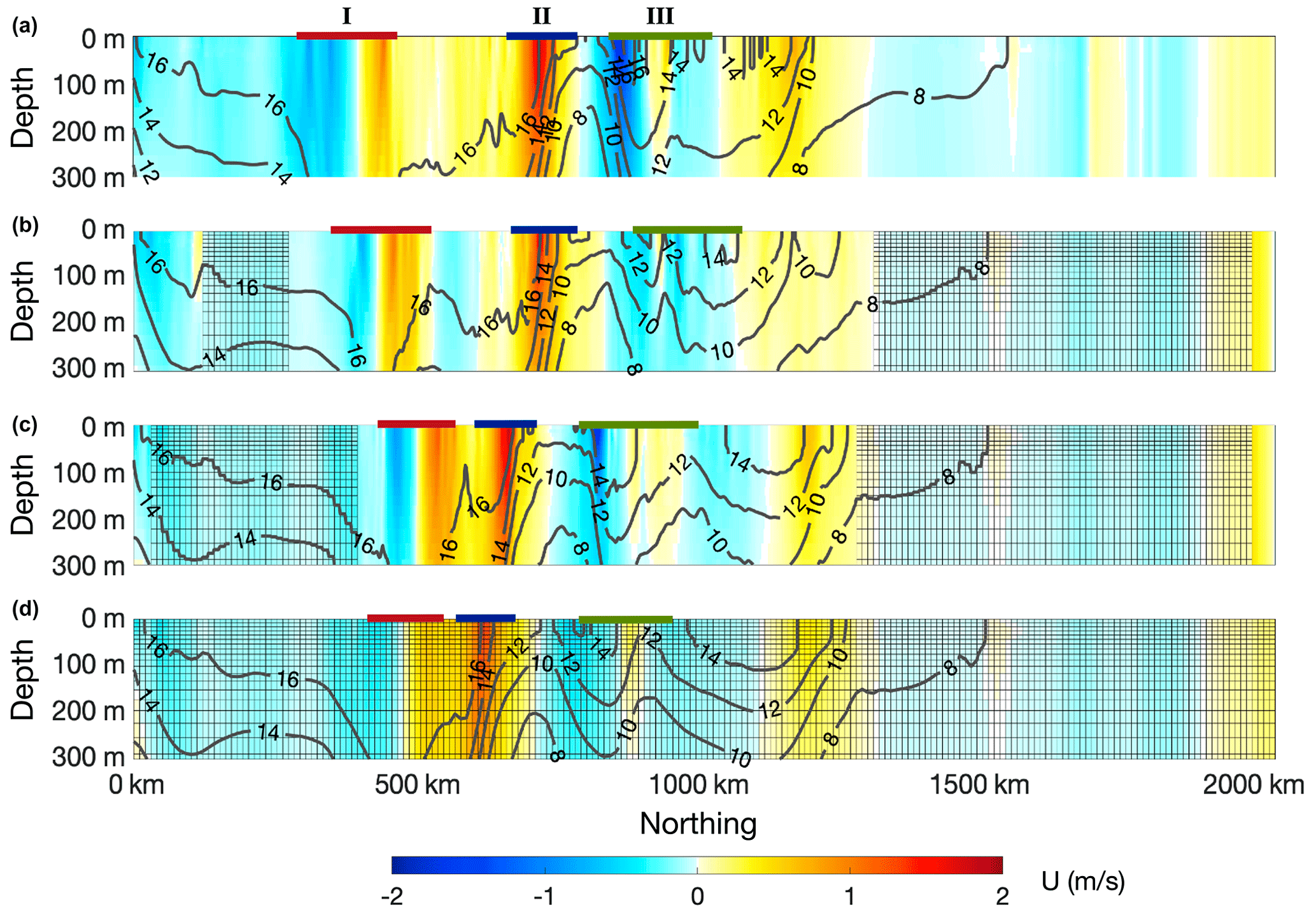
Figure 14 Typical meridional–vertical transects (top 300 m) in Fig. 12. Temperature (contour lines) and zonal velocity (filled contour) are shown in each panel. The four experiments, S, M-S-I, M-S-I, and M, are shown in order from (a) to (d). Grids in the lower three panels show the region with 0.1^∘ resolution (i.e., not refined). In each panel, the three features are marked: I for the mesoscale eddy in the subtropical gyre, II for the core of the western-boundary current, and III for the submesoscale-rich region to the north of II.

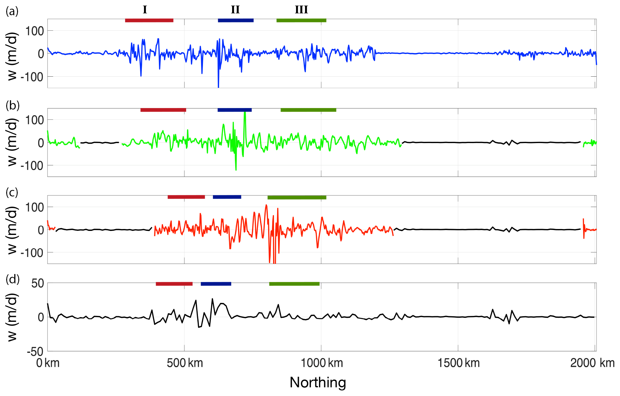
Figure 15 Vertical speed (w, m d⁻¹) at 50 m depth (k=7) on the meridional–vertical transects in Fig. 14. Panel layout, as well as the three features, is the same as in Fig. 14. In (b)–(d), the region with 0.1^∘ (0.02^∘) resolution is marked by black lines (colored lines). Note that the range is different in (d) due to the overall smaller vertical speed in the full-field 0.1^∘ experiment (i.e., M).

4 Summary and discussion

4.1 Summary

We present OMARE, an ocean modeling framework with adaptive spatial refinement based on NEMO, with the initial results based on an idealized double-gyre test case. Compared with AGRIF-based NEMO, we adopt a piece of third-party software middleware, JASMIN, to satisfy various modeling needs. JASMIN provides NEMO with the service of adaptive refinement, as well as an abstraction layer that shields away details of domain decomposition, parallel computing, and model output. This paper mainly focuses on the porting of NEMO onto JASMIN, as well as the ocean physics at three resolutions of 0.5, 0.1, and 0.02^∘, which are typical in climate studies and high-resolution simulations. We investigate in particular the (adaptive) mesh refinement with these resolutions in a double-gyre test case which simulates a western-boundary current system. Another accompanying paper will further introduce the computational aspects of OMARE, including the scalability and computability of OMARE, with a particular focus on AMR and its role in improving the computational efficiency of high-resolution simulations.

The code refactorization onto JASMIN involves a non-trivial process of mixed-language programming with FORTRAN and C++. The major work is divided into two parts: (1) to transform the NEMO into decomposition-free components that satisfy JASMIN's protocols and (2) to rewrite the time integration in C++ with JASMIN. JASMIN components are elements for communication (i.e., boundary exchanges) and computation. We follow the JASMIN routines and refactor both the dynamic core of NEMO and the various physical parameterization schemes that are needed for the three resolutions. In total, the refactorization yields 155 JASMIN components and 422 JASMIN patches, with over 30 000 lines of code (in both FORTRAN and C++). The refactorization process in total involves about 32 person months to finish. For comparison, for AGRIF-based NEMO, the time integration is also managed externally (i.e., by AGRIF), but the overall integration is similar to an “add-on” to NEMO and relatively lighter in terms of coding compared with OMARE. In addition, the parallel input/output and restart is managed through JASMIN, instead of a standalone library of XIOS in NEMO (or AGRIF-based NEMO).

For the ocean physics as modeled with OMARE, with the refinement from 0.5 to 0.1^∘, the model simulates drastically different physical processes, from laminar to mesoscale-rich, turbulent ocean. Boundaries between the two resolutions act as a lateral forcing for the 0.1^∘ region, providing boundary conditions for the refined region through both spatial and temporal interpolations. As a result, both the mean status in the subpolar and subtropical gyres and the ocean dynamics at 0.1^∘ are directly affected by the status simulated with 0.5^∘. The higher potential energy at lower resolution is also witnessed in Marques et al. (2022) (Fig. 3 of the reference showing higher PE at $\mathrm{1}/\mathrm{4}{}^{\circ }$ than higher resolutions). This is consistent with our study, indicating that in low-resolution models, the energy is removed by grid-scale diffusion and not effectively converted to kinetic energy, hence causing the accumulation of PE.

We further demonstrate the adaptive refinement from 0.1 to 0.02^∘, focusing on the temporally changing processes on WBC. With the threshold-value-based refinement criteria of velocity and relative vorticity, the model grasps the major mesoscale features on WBC. Furthermore, reasonable submesoscale processes are simulated by refining to 0.02^∘ and, in particular, their seasonality. Outstanding issues include the inconsistencies across the resolution boundaries beyond the mesoscale predictability, as well as the ensuing numerical noises. These issues, among other related topics, are further addressed in the discussion below.

4.2 Refining criteria and frequency for AMR

The refinement criterion for AMR is an open question for simulating the ocean's multi-scale processes. In Sect. 3.4 we showed that the instantaneous surface velocity and vorticity at 0.1^∘ serve as good proxies for mesoscale processes on WBC. Further improvements to the criteria can be achieved by introducing memory and predictive capabilities to better capture the mesoscale features. In addition, the threshold values can be further improved instead of the percentiles in Sect. 3.4, such as a prescribed KE amount/percentage with AMR. Instead of AMR, a prescribed refinement region based on a priori knowledge is another type of criterion (Sect. 3.3). OMARE supports both types of refinement (dynamic or static), through a generalized interface for marking arbitrary grid cells for refinement. Specifically, a prescribed parameter for refinement granularity can be used to control the patch size on the refined region, ensuring both the full coverage to these marked grid cells and patch sizes, which affects computational performance. Due to the inherent turbulence of the ocean's mesoscale, the specific regions of interest, such as mesoscale eddies, WBC meandering, and ocean fronts, are temporally changing and have process-dependent predictability. Therefore, the support for AMR in OMARE ensures the flexibility in future application in various modeling scenarios and processes of even finer temporal/spatial scales.

The update frequency of the dynamically changing refined region is another key parameter for AMR. For the refinement from 0.1 to 0.02^∘, we use 5 d as the update interval (i.e., super cycle). This interval should be no larger than the temporal scale of the process to be studied – here the mesoscale processes. In general, with longer intervals, the refinement region should also be enlarged, in order to accommodate the changes in the locations for the regions of interest. Another contributing factor is the computational overhead associated with adjusting the refinement region. For OMARE and JASMIN, this overhead includes the domain decomposition and (re)mapping to processors, the establishment of communication framework, and the associated model state migration and interpolations. We will further examine the computational behavior of various AMR scenarios in Part 2 of this paper.

4.3 Boundary exchanges

For the lateral boundaries between coarse and fine resolutions, we have implemented bilinear interpolators for both state variables on the outer boundaries (i.e., T, sea-surface height, among others) of the fine-resolution grid and fluxes on the boundaries (i.e., u and v). For temporal interpolation, a simple linear interpolation is utilized, with support for both barotropic and baroclinic steps. Better, more sophisticated schemes are available from the established works involving NEMO and AGRIF. In particular, Debreu et al. (2012) have meticulously designed conservative interpolators, filters and the sponge layer, and specific treatments for the split-explicit formulation of the dynamic core. In future work, we plan to investigate and implement improved interpolators and further evaluate their numerical behavior in OMARE.

4.4 Upscaling in refinement settings

Another future improvement to OMARE is the feedback of the model status from the refined region to the non-refined region. In OMARE, in the region covered by a fine-resolution grid, the model still carries out simulation with the coarse resolution. A simple updating scheme can be implemented, as follows: (1) coarsening the model status in the refined region and (2) overwriting the model status on the coarse resolution. The updating process can lower the inconsistency of the two resolutions on the boundaries, hence reducing the noises as observed in Sect. 3.4. In addition, small-scale processes are unresolved and parameterized on the coarse resolution. Therefore, from the physics perspective, the update also corresponds to an “upscaling” process. The refinement to a finer resolution yields more trustworthy model status due to explicitly resolving these processes. The updating then potentially improves the model status on the coarse resolution, hence the effect of upscaling. Moreover, instead of directly overwriting the model status on the coarse resolution, data-assimilated assisted approaches can be applied, such as nudging and variational methods. Due to the inherently different ocean dynamics and even mean states as simulated by different resolutions (e.g., Sect. 3.3, Levy et al., 2010), how to improve the coarse-resolution model with refinement remains an open and daunting task. With AMR in representative regions and the upscaling capability of OMARE, we plan to carry out studies of key processes, including the effect of the restratification by submesoscale processes on the mean status (Levy et al., 2010; Pennelly and Myers, 2020).

4.5 Ocean physics in double-gyre and related idealized cases

The double-gyre case is typical of wind-driven ocean circulation in the midlatitude. There are several aspects of the case and the corresponding model configurations that need further improvements. Unlike the two WBC systems in the Earth's Northern Hemisphere, the Kuroshio and the Gulf Stream, the double gyre is limited in size, especially in the meridional direction. This compromises the comparability to the realistic WBC systems, since we have witnessed prominent boundary-related mesoscale and associated submesoscale processes for the double-gyre case in this study (Sect. 3.4). Furthermore, the lateral boundary condition is uniformly free-slip in all experiments, which in effect inhibits the energy dissipation through lateral friction. However, the best lateral boundary condition for ocean models, and specifically, for NEMO, remains elusive and therefore is subject to tuning to specific model settings, as well as targeted observations. Given the complex bathymetry for continental shelf in realistic cases, there may be no general rule for the best lateral boundary condition. OMARE, with the grid refinement on lateral boundaries and upscaling, can be utilized to study eddy current–bathymetry interactions, as well as the effective lateral boundary condition.

Another aspect that needs improvements in OMARE is the specific choices of parameterization schemes and parameters. Lateral mixing schemes, such as GM90 (Gent and McWilliams, 1990), are widely used in non-eddying (i.e., laminar) ocean models in order to approximate the effect of mesoscale eddies and improve the model's simulation of isopycnal mixing. In OMARE, we currently use a simple, first-order Laplacian mixing scheme for the sake of simplicity. At higher resolutions (0.1 and 0.02^∘), we adopt the second-order mixing scheme with adaptation to grid cell sizes. The parameters are prescribed from standard runs and should be scrutinized for further tuning of the model. This also applies to the TKE scheme for vertical mixing, which is used across all three resolutions.

The double gyre as used in this study belongs to a series of idealized test cases for ocean models, such as Levy et al. (2010) and Marques et al. (2022). In particular, the rotation of the gyre to be the purely zonal–meridional direction from Levy et al. (2010) enables a more regularly shaped system, but its polar branch is disabled. Also in Marques et al. (2022), the authors propose an idealized case of intermediate complexity, which contains the Northern and Southern Hemisphere, the tropical ocean, as well as the circumpolar circulation with an east–west periodic boundary condition. However, the atmospheric forcing in Marques et al. (2022) does not contain a seasonal cycle. For comparison, the seasonal cycle of the forcing in this study enables the simulation of the seasonality of submesoscale activities.

4.6 Realistic cases

In order to carry out simulation of Earth's ocean with OMARE, realistic bathymetry, ocean states, and historical atmospheric forcings should be incorporated in OMARE. Specifically, spatial refinement can be carried out in key regions with bathymetric features, such as land–sea boundaries, continental shelves, and sea mounts. Due to the different bathymetry across the resolutions in OMARE, the model status on the coarse grid contains inherent inconsistencies for the refined region. Therefore, after spatial and temporal interpolations, the lateral boundary conditions to the refined region need to be modified accordingly, in order to reduce any potential physical or numerical issues. In addition, a prognostic, fully thermodynamic and dynamic sea ice component is also needed, such as SI³ (Vancoppenolle et al., 2023), which is a module in the surface boundary condition (SBC) of NEMO. We plan to incorporate sea ice in the future version of OMARE, as well as other relevant processes, including tide and wind wave. Both static and adaptive refinement can be further utilized for the study of the key regions and/or multi-scale processes of the global ocean.

Appendix A: Atmospheric forcings for the double-gyre case

The atmospheric forcing of the double-gyre case contains the wind stress forcing and the thermodynamic forcing which both contain an annual cycle. Each model year contains 360 d. The wind stress is purely zonal (i.e., τ_x, in N m⁻²) and a function of both latitude (ϕ, in radians) and time of the year (t, normalized between 0 and 1 within the year), as shown in Eq. (A1). The meridional wind stress is constantly 0 N m⁻². The thermodynamic forcing also follows a meridional structure and is enforced on the model's surface through a restoring condition to the predefined annual cycle of apparent temperature, SST_f, defined in Eq. (A2). The restoring strength is −40 Wm⁻² K⁻¹. Total surface heat flux (i.e., Q_tot, split into solar part Q_sr and non-solar part Q_ns, both in Wm⁻²) is in proportion to SST_f− SST, with SST the model's instantaneous surface temperature. Q_tot is defined in Eq. (A3), following Levy et al. (2010). Solar heat flux Q_sr in Eq. (A4) penetrates into seawater, while non-solar heat flux Q_ns only influences the surface layer of the model. The most extreme conditions of τ_x and SST_f during winter and summer are shown in Fig. 5.

In order to maintain the overall hydrological balance within the basin, we compensate for the imbalance in fresh water with the basin-mean value of evaporation minus precipitation (EMP). In the case of refinement experiments (including AMR), we only compute the areal-mean value of EMP on the coarsest resolution and use it as the freshwater forcing across the all resolution levels.

$$\begin{array}{}\text{(A1)}& {\displaystyle }\begin{array}{rl}{\mathit{\tau }}_x(\mathit{\varphi },t)& =\mathrm{8.7}\cdot {\mathrm{10}}^{-\mathrm{4}}\left(\right(\cos (\mathrm{2}\mathit{\pi }t-\mathrm{0.79})+\mathrm{12}){)}^{\mathrm{2}}\\ & \cdot \sin (\mathrm{0.38}\mathit{\varphi }-\mathrm{6.82}+\mathrm{0.5}\cos (\mathrm{2}\mathit{\pi }t-\mathrm{0.79}\left)\right)\end{array}\text{(A2)}& {\displaystyle }{\mathrm{SST}}_f(\mathit{\varphi },t)=\mathrm{28.3}\cdot {\displaystyle \frac{\begin{array}{c}(\mathrm{1}+\mathrm{0.02}\cdot \cos (\mathrm{2}\mathit{\pi }(t-\mathrm{0.558})\left)\right)\\ \cdot \cos (\mathit{\pi }\cdot \mathit{\varphi }-\mathrm{5})\end{array}}{\mathrm{107}+\mathrm{22.5}\cdot \cos \left(\mathrm{2}\mathit{\pi }\right(t-\mathrm{0.558}\left)\right))}}\text{(A3)}& {\displaystyle }\begin{array}{rl}{Q}_{\mathrm{tot}}(\mathit{\varphi },t)& =-\mathrm{40}\cdot \left({\mathrm{SST}}_f\right(\mathit{\varphi },t)-\mathrm{SST}(\mathit{\varphi },t\left)\right)\\ & =Q_{\mathrm{sr}}(\mathit{\varphi },t)+Q_{\mathrm{ns}}(\mathit{\varphi },t)\end{array}\text{(A4)}& {\displaystyle }\begin{array}{rl}{Q}_{\mathrm{sr}}(\mathit{\varphi },t)& =\mathrm{230}\cdot \cos (\mathrm{0.019}\cdot \mathit{\varphi }-\mathrm{0.447}\\ & \cdot \cos \left(\mathrm{2}\mathit{\pi }\right(t-\mathrm{0.475}\left)\right))\end{array}\end{array}$$

Appendix B: Spatial scaling for the computation of vorticity and velocity

We show the computing of relative vorticity related spatial derivatives with the two-dimensional velocity fields and Arakawa-C grid staggering. The relative vorticity (ζ) at a certain spatial scale is defined as the combination of two derivatives at the specific scale: $\mathit{\zeta }=-\frac{\partial u}{\partial y}+\frac{\partial v}{\partial x}$. The two derivatives are formally defined by line integrals over a certain area A with the corresponding spatial scale of $\sqrt{A}$, as in Eqs. (B1) and (B2).

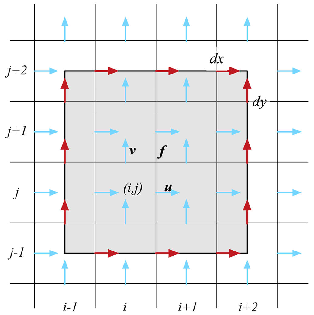
Figure B1 Spatial scaling of 3×3 cells with Arakawa-C grid staggering. All velocities used during the computation of line integrals are marked by red arrows, with others marked by blue.

For NEMO with Arakawa-C grid staggering in the horizontal direction, the relative vorticity is computed on the f point (or north–east corner) of each cell. Figure B1 shows the case of spatial scaling with nine grid cells (i.e., 3×3) at the grid location (i, j). Velocities of adjacent 16 cells are utilized to compute the two scaled derivatives of $\frac{\partial u}{\partial y}$ and $\frac{\partial v}{\partial x}$.

For the general case of computing the scaled version of relative vorticity (denoted $\stackrel{\mathrm{̃}}{\mathit{\zeta }}$) for the grid points from i=i₁ to i₂ in the x direction and from j=j₁ to j₂ in the y direction, we compute it following Eq. (B3). In Eq. (B3), the cell lengths of the f points are denoted dx_i,j and dy_i,j in the x direction and y direction, respectively. The corresponding spatial scale is then computed as the square root of the total area, i.e., $\sqrt{{\sum }_{i,j}(\mathrm{d}{x}_{i,j}\cdot \mathrm{d}{y}_{i,j})}$.

For determining the refinement region for AMR, for every cell in the grid, we compute the scaled values of the relative vorticity and the velocity, at the scale of 5×5 grid cells. These values are compared against prescribed threshold values. With spatial scaling, the line integral should traverse valid model cells. In the case of the area A covering invalid cells (i.e., land), Eq. (B3) should be adjusted accordingly. For the sake of simplicity, by default, we mark the cells that are adjacent to the lateral boundaries for refinement in this study.

$$\begin{array}{}\text{(B1)}& {\displaystyle \frac{\partial u}{\partial y}}{|}_{\mathrm{scale}=\sqrt{A}}=-{\displaystyle \frac{\mathrm{1}}{A}}\oint u\cdot \mathrm{d}x\text{(B2)}& {\displaystyle \frac{\partial v}{\partial x}}{|}_{\mathrm{scale}=\sqrt{A}}={\displaystyle \frac{\mathrm{1}}{A}}\oint v\cdot \mathrm{d}y\text{(B3)}& {\displaystyle }\stackrel{\mathrm{̃}}{\mathit{\zeta }}{|}_{i_{\mathrm{1}},i_{\mathrm{2}};j_{\mathrm{1}},j_{\mathrm{2}}}={\displaystyle \frac{\begin{array}{c}{\sum }_{i=i_{\mathrm{1}}}^{i_{\mathrm{2}}}{u}_{i,j_{\mathrm{1}}-\mathrm{1}}\mathrm{d}{x}_{i,j_{\mathrm{1}}-\mathrm{1}}-{\sum }_{i=i_{\mathrm{1}}}^{i_{\mathrm{2}}}{u}_{i,j_{\mathrm{2}}}\mathrm{d}{x}_{i,j_{\mathrm{2}}}\\ +{\sum }_{j=j_{\mathrm{1}}}^{j_{\mathrm{2}}}{v}_{i_{\mathrm{2}},j}\mathrm{d}{y}_{i_{\mathrm{2}},j}-{\sum }_{j=j_{\mathrm{1}}}^{j_{\mathrm{2}}}{v}_{i_{\mathrm{1}}-\mathrm{1},j}\mathrm{d}{y}_{i_{\mathrm{1}}-\mathrm{1},j}\end{array}}{{\sum }_{i=i_{\mathrm{1}}}^{i_{\mathrm{2}}}{\sum }_{j=j_{\mathrm{1}}}^{j_{\mathrm{2}}}\mathrm{d}{x}_{i,j}\cdot \mathrm{d}{y}_{i,j}}}\end{array}$$