The effect of emission source chemical profiles on simulated PM_2.5 components: sensitivity analysis with the Community Multiscale Air Quality (CMAQ) modeling system version 5.0.2

A chemical transport model (CTM) is an essential tool for air quality prediction and management, widely used in air pollution control and health risk assessment. However, the current models do not perform very well in reproducing the observations of some major chemical components, for example, sulfate, nitrate, ammonium and organic carbon. Studies have suggested that the uncertainties in the model chemical mechanism, source emission inventory and meteorological field can cause inaccurate simulation results. Still, the emission source profile (used to create speciated emission inventories for CTMs) of PM_2.5 has not been fully taken into account in current numerical simulation. Based on the characteristics and variation rules of chemical components in typical PM_2.5 sources, different simulation scenarios were designed and the sensitivity of simulated PM_2.5 components to the source chemical profile was explored. Our findings showed that the influence of source profile changes on simulated PM_2.5 components' concentrations cannot be ignored. Simulation results of some components were sensitive to the adopted source profile in CTMs. Moreover, there was a linkage effect: the variation in some components in the source profile would bring changes to the simulated results of other components. These influences are connected to chemical mechanisms of the model since the variation in species allocations in emission sources can affect the potential composition and phase state of aerosols, chemical reaction priority, and multicomponent chemical balance in thermodynamic equilibrium systems. We also found that the perturbation of the PM_2.5 source profile caused variation in simulated gaseous pollutants, which indirectly indicated that the perturbation of source profile would affect the simulation of secondary PM_2.5 components. Our paper highlights the necessity of paying enough attention to the representativeness and timeliness of the source profile when using CTMs for simulation.

1 Introduction

Ambient fine particulate matter (PM_2.5) pollution in some key regions of China has attracted much attention (Liang et al., 2020; Huang et al., 2021). The chemical components of PM_2.5, including elements (Al, Si, Fe, Mn, Ti, Cu, Zn, Pb, etc.), water-soluble ions (SO${}_{\mathrm{4}}^{\mathrm{2}-}$, NO${}_{\mathrm{3}}^{-}$, Cl⁻, F⁻, NH${}_{\mathrm{4}}^{+}$, Na⁺, K⁺, Mg²⁺, Ca²⁺, etc.) and carbon-containing components (organic carbon, OC; elemental carbon, EC) (Yang et al., 2011; Li et al., 2013), have different physical and chemical properties, such as reactivity, thermal stability, particle size distribution, residence time, optical properties or health hazards (Seinfeld and Pandis, 2006; Tang et al., 2006). According to long-term monitoring results, in most regions of China, SO${}_{\mathrm{4}}^{\mathrm{2}-}$, NO${}_{\mathrm{3}}^{-}$, NH${}_{\mathrm{4}}^{+}$ and OC are the most important species in ambient PM_2.5 (Li et al., 2017a, 2021), which has a certain adverse impact on human health (Shi et al., 2018) and ecosystems, such as acid rain in southwest China (Han et al., 2019) or food security (Zhou et al., 2018).

Chemical transport models (CTMs) play an important role in policymaking for regulatory purposes. Based on the scientific understanding of atmospheric physical and chemical processes, CTMs are built to simulate the transport, reaction and removal of pollutants on a certain scale in horizontal and vertical directions. With the development of CTMs, the simulation accuracy of PM_2.5 concentration has been significantly improved. Higher requirements have been put forward for the precise simulation of PM_2.5 components so as to provide support for the use of CTMs in human health risk assessment, climate effects, pollution sources apportionment and so on (Peterson et al., 2020; Lv et al., 2021). However, the current models do not perform very well in simulating some components (for example, PM_2.5-bound sulfate, nitrate, ammonium, trace elements) (Zheng et al., 2015; Fu et al., 2016; Ying et al., 2018; Cao et al., 2021). In the current literature, the correlation coefficient (R) and normalized mean bias (NMB) are highly variable and inconsistent between the simulated and the observed values (listed in Table S1 in the Supplement). This is mainly attributable to the uncertainties in the model chemical mechanism, source emission inventory and meteorological field simulation.

The chemical mechanisms involved in CTMs are derived from parameterized assumptions based on laboratory simulation and field observations. The actual atmospheric chemical processes are very complex, and some reaction mechanisms are still limitedly understood. In addition, the integration of chemical reactions and simplified treatment methods in the model cannot fully reflect the correlation among atmospheric pollutants. For example, in some model mechanisms, important sulfate and nitrate formation pathways through new heterogeneous chemistry were added, including the chemical reaction between SO₂ and aerosol, ${\mathrm{NO}}_{\mathrm{2}}/{\mathrm{NO}}_{\mathrm{3}}/{\mathrm{N}}_{\mathrm{2}}{\mathrm{O}}_{\mathrm{3}}$ and aerosol (Zheng et al., 2015); nitrous acid oxidizing SO₂ to produce sulfate (Zheng et al., 2020); dust particles promoting the oxidation of SO₂ (Yu et al., 2020); modifying the uptake coefficients for heterogeneous oxidation of SO₂ to sulfate (Zhang et al., 2019); and updating the heterogeneous N₂O₅ parameterization (Foley et al., 2010). Even though the aforementioned processes can significantly improve the simulation of SO${}_{\mathrm{4}}^{\mathrm{2}-}$ and NO${}_{\mathrm{3}}^{-}$, there is still a gap between the modeled and the actual atmospheric chemical processes.

The uncertainty in meteorological field simulation is another crucial reason for the simulation deviation; especially on heavy-pollution days, the variation trends of PM_2.5 chemical components were not well-captured (Ying et al., 2018; Qi et al., 2019; Wang et al., 2022). Precipitation is the key meteorological factor determining wet removal of pollutants; boundary layer height and wind speed are the main factors affecting convection and transport of pollutants; solar radiation, temperature and relative humidity are the key factors affecting the formation of secondary particles (Huang et al., 2019; Chen et al., 2020). Some literature has reported that deviation from precipitation and wind field simulation might lead to underestimation of SO${}_{\mathrm{4}}^{\mathrm{2}-}$, NO${}_{\mathrm{3}}^{-}$ and NH${}_{\mathrm{4}}^{+}$ (Cheng et al., 2015; Zhang et al., 2017). Devaluation of the liquid water path and cloud cover causes a decrease in sulfate formation in cloud and ultimately results in significantly underestimated components in simulation values (Sha et al., 2019; Foley et al., 2010). Underestimation of temperature and relative humidity may also cause adverse effects of the temperature-dependent and/or relative-humidity-dependent chemical reaction in the simulation (Sha et al., 2019).

The uncertainty in the source emission inventory also significantly affects the simulation results of PM_2.5 components (Shi et al., 2017; Sha et al., 2019). Due to incomplete information or insufficient representativeness, pollutant emissions are sometimes overestimated or underestimated, and the method for temporal and spatial allocation also needs to be improved.

In particular, the emission source profile of PM_2.5 (hereinafter referred to as the “source profile”), used to create speciated emission inventories for CTMs (Hsu et al., 2019), has not been fully taken into account in the current numerical simulation. In the reported literature, PM_2.5 species allocation coefficients of emission sources are commonly treated in the following ways: (1) allocating PM_2.5 components of source emissions by referring to source profile data in published literature or databases like US SPECIATE (Fu et al., 2013; Wang et al., 2014; Ying et al., 2018) and (2) determining chemical profiles from local measurement (Fu et al., 2013; Appel et al., 2013). However, with the development of production technology and the innovation of pollution treatment technology in recent years, some source profiles have changed dramatically (Bi et al., 2019a), such as SO${}_{\mathrm{4}}^{\mathrm{2}-}$ from coal burning: its content in PM_2.5 is generally low in coal-fired power plants without desulfurizing facilities, while existing coal-fired power plants use limestone–gypsum wet desulfurization, and the contents of SO${}_{\mathrm{4}}^{\mathrm{2}-}$ in PM_2.5 are significantly higher than those without desulfurization facilities (Zhang et al., 2020). The timeliness of PM_2.5 species allocation coefficients in current CTMs also needs to be considered.

This paper attempts to answer the following questions: (1) whether the variation in the source profile adopted in the model has an impact on the simulated results of PM_2.5 chemical components. (2) How large is that impact? (3) How does the impact work? Aiming to address these problems above, chemical composition and its variation law for typical PM_2.5 emission sources are summarized; on this basis, sensitivity tests are designed to identify whether PM_2.5 source profiles and species allocation in the model are important parameters that affect the simulation results of chemical components' concentrations in PM_2.5. We take the Community Multiscale Air Quality model (CMAQ, one of the most widely used CTMs) and the Multi-resolution Emission Inventory for China (MEIC, a high-resolution inventory of anthropogenic air pollutants in China) as the carriers. The same kind of experiment is also applicable to other CTMs and emission inventories. The aim of this study is to provide support for the effective utilization of source profiles in the CTMs and improvement of the simulation schemes.

2 Model and data

2.1 Model configuration

The Weather Research and Forecasting model (WRF 3.7.1), the widely used Community Multiscale Air Quality model (CMAQv5.0.2) (Eder and Yu, 2006; Yu et al., 2014), and the Multi-resolution Emission Inventory for China (MEICv1.3) have been used in this study. MEIC, developed by Tsinghua University, mainly tracked anthropogenic emissions in China including coal-fired power plant, industry, vehicle, residential and agricultural sources (http://meicmodel.org/?page_id=135, last access: 14 November 2023) (Li et al., 2017b; Zheng et al., 2018). The WRF model was used to generate meteorological inputs for the CMAQ model. Three nested modeling domains consisting of 36 km × 36 km (Dom1), 12 km × 12 km (Dom2) and 4 km × 4 km (Dom3) horizontal grid sizes were set, as shown in Fig. 1. The initial and boundary conditions for WRF were based on the North American Regional Reanalysis data archived at National Center for Atmospheric Research (NCAR). In addition, surface and upper-air observations obtained from NCAR were used to further refine the analysis data. The modeling was conducted from 1 to 30 October 2018, and the major configurations we used in CMAQ were as follows: gas-phase chemistry was based on the CB05 mechanism, and the aerosol dynamics and chemistry were based on the AERO6 module (cb05tucl_ae6_aq). The detailed model configurations are shown in Table S2, and the regional distribution of PM_2.5 emission sources is shown in Fig. S1.

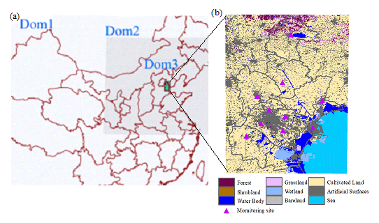
Figure 1 Modeling domains of the CMAQ model. (a) The three-domain nested CMAQ domains. (b) Land use and observation sites of Dom3 (data source of land use: GlobeLand30, https://www.webmap.cn/mapDataAction.do?method=globalLandCover, last access: 14 November 2023, National Geomatics Center of China).

2.2 Selection and comparison of the PM_2.5 emission source profile

The PM_2.5 emission source profiles from the database of Source Profiles of Air Pollution (SPAP) (http://www.nkspap.com:9091/, last access: 14 November 2023) and the US Environmental Protection Agency (EPA) SPECIATE database (https://www.epa.gov/air-emissions-modeling/speciate, last access: 14 November 2023) as well as from the published literature were selected. SPAP was developed by the State Environment Protection Key Laboratory of Urban Particulate Air Pollution Prevention, Nankai University, China. This database contains more than 3000 size-resolved source profiles of stationary combustion sources, industrial processes, vehicle exhaust, biomass burning, dust and other sources, collected from more than 40 cities in China since 2001. In addition to inorganic elements, water-soluble ions, OC, EC and other conventional components, some source profiles also encompass tracer information, such as organic markers, isotopes, single-particle mass spectrometry, volatile organic compounds (VOCs) and other gaseous precursors. Based on species in the aerosol chemical mechanism (AERO6) of CMAQ (Appel et al., 2013; Chapel Hill, 2012), we selected 15 components in PM_2.5 source profiles including Al, Ca, Cl, EC, Fe, K, Mg, Mn, Na, OC, Si, Ti, NH${}_{\mathrm{4}}^{+}$, NO${}_{\mathrm{3}}^{-}$ and SO${}_{\mathrm{4}}^{\mathrm{2}-}$; the remaining components are classified as “other”. In the database of Source Profiles of Air Pollution (SPAP) and the US EPA SPECIATE database, the four source categories (coal-fired power plant, industry process, transportation sector and residential coal combustion) contain a series of sub-categories. But MEIC does not include the corresponding sub-categories. So we take the average values of source profiles in each source category as representing the source profile; the details can also be seen in our previous work (Bi et al., 2019a). Then we multiply inventory emissions by profile fraction to get emissions of specific chemical components.

To determine the similarity between the two groups of source profiles. The coefficient divergence (CD) is calculated using the following formula (Wongphatarakul et al., 1998):

$$\begin{array}{}\text{(1)}& {\mathrm{CD}}_{jk}=\sqrt{{\displaystyle \frac{\mathrm{1}}{p}}{\sum }_{i=\mathrm{1}}^p{\left({\displaystyle \frac{x_{ij}-x_{ik}}{x_{ij}+x_{ik}}}\right)}^{\mathrm{2}}},\end{array}$$

where CD_jk is the coefficient of divergence of the source profile j and k, p is the number of chemical components in the source profile, x_ij is the weight percentage for the chemical component i in source profile j, and x_ik is the weight percentage for i in source profile k (%). The CD value is in the range of 0 to 1; if the two source profiles are similar, the value of CD is close to 0, and if the two are very different, the value is close to 1.

2.2.1 Coal-fired power plant (PP)

Coal-fired power plants remain the main coal consumers in China and accounted for 50.2 % of total coal consumption in 2019 (NBS, 2021). They have gained much attention, especially with the wide implementation of the ultralow emission standards by which PM_2.5 emission characteristics have changed accordingly (Wu et al., 2020, 2022). There are obvious differences in PM_2.5 source profiles between SPAPPC (SPAP database and published source profiles in China) and SPECIATE (US EPA SPECIATE database); the CD value of these two groups lies between 0.34 and 0.92 (0.64 ± 0.10). Detailed information is shown in Table S3 and Fig. S2 in the Supplement. The percentages of species in PP source profiles are plotted in Fig. 2a. The main components in SPAPPC are sorted by Si, SO${}_{\mathrm{4}}^{\mathrm{2}-}$, OC and Ca with average values of 8.7 ± 6.8 %, 8.5 ± 11.5 %, 6.8 ± 9.1 % and 6.5 ± 6.9 %, respectively. The SPECIATE data are enriched in SO${}_{\mathrm{4}}^{\mathrm{2}-}$ (16.9 % ± 20.0 %), OC (12.7 ± 21.8 %), Si (9.6 ± 5.0 %) and Ca (9.3 ± 7.3 %), which are higher than SPAPPC. Coal properties, burning conditions, pollution control measures and emission sampling methods are the main reasons for those great percentage fluctuations. Different treatment processes of flue gases, e.g., wet/dry limestone, ammonia and double-alkali flue gas desulfurization, will affect the percentages of components in source profiles (Zhang et al., 2020). It has been reported that the percentage of Ca, Mg, SO${}_{\mathrm{4}}^{\mathrm{2}-}$ and Cl⁻ in PP profiles increased after the limestone–gypsum method was used in coal-fired power plants (Bi et al., 2019a). Besides that, the percentage of Cl⁻ in SPAPPC is obviously higher than that in SPECIATE, which might be attributed to the generally higher Cl⁻ content in raw coal in China (Guo et al., 2004).

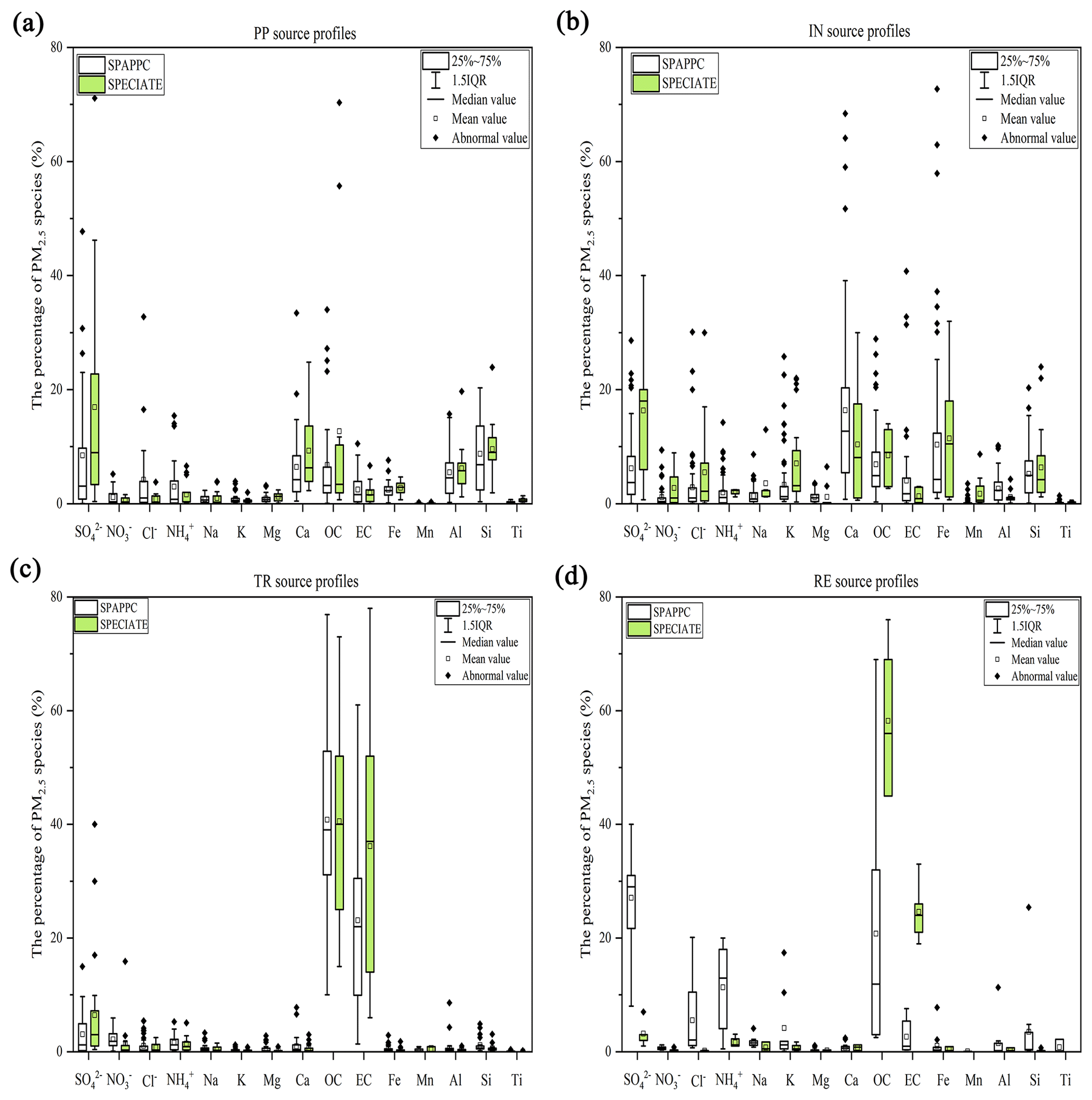
Figure 2 Chemical profiles for PM_2.5 emitted from (a) coal-fired power plants (PP), (b) industry processes (IN), (c) the transportation sector (TR) and (d) residential coal combustion (RE). Data obtained from SPAPPC (SPAP database and published source profiles in China) and SPECIATE (US EPA SPECIATE database).

2.2.2 Industrial process (IN)

Industrial emissions are one of the major sources of PM_2.5 (Hopke et al., 2020); the percentages of Ca, Fe, OC and SO${}_{\mathrm{4}}^{\mathrm{2}-}$ are relatively high in both SPAPPC and SPECIATE, but the shares in different source profile databases vary. Their CD values vary from 0.45 to 0.94 (0.72 ± 0.09) (detailed information is shown in Tables S4–S7 and Fig. S3). In SPAPPC, these four components account for 16.4 ± 14.9 %, 10.4 ± 14.4 %, 6.9 ± 6.1 % and 6.2 ± 6.4 %; the proportions in SPECIATE are 10.4 ± 9.8 %, 11.4 ± 10.6 %, 8.5 ± 4.9 % and 16.3 ± 13.3 %, respectively (Fig. 2b). Large variations in components and their percentages in industrial processes are attributed to the manufacturing processes, raw material, pollution control measures and so on (Ji et al., 2017; Bi et al., 2019a; Gao et al., 2022). For example, Ca, Al, OC and SO${}_{\mathrm{4}}^{\mathrm{2}-}$ are found to have the highest percentages in cement sources (Guo et al., 2021); Fe, Si and SO${}_{\mathrm{4}}^{\mathrm{2}-}$ are the most abundant species in steel industry emissions (Guo et al., 2017).

2.2.3 Transportation sector (TR)

Traffic contributed a large fraction of PM_2.5 in many locations (Hopke et al., 2022). It is well-known that the transportation sector makes a dominant contribution of OC and EC. The main components of PM_2.5 emitted from traffic sources are OC, EC and SO${}_{\mathrm{4}}^{\mathrm{2}-}$ in both SPAPPC and SPECIATE, but they still vary in a wide range: their CD values fall between 0.33 and 0.86 (0.69 ± 0.09) (detailed information is given in Tables S8–S10 and Fig. S4). In SPAPPC, the percentages of OC, EC and SO${}_{\mathrm{4}}^{\mathrm{2}-}$ are 40.8 ± 15.0 %, 23.1 ± 13.8 % and 3.1 ± 3.7 %, and in SPECIATE, the percentages are 40.6 ± 16.4 %, 36.1 ± 21.5 % and 6.4 ± 9.9 %, respectively (Fig. 2c). These significant differences can mainly be attributed to the vehicle type, fuel quality, mixing ratio between oil and gas, and combustion phase in vehicle engine (Xia et al., 2017).

2.2.4 Residential coal combustion (RE)

Residential coal combustion, as the leading source of global PM_2.5 emissions (Weagle et al., 2018), has a much higher emission factor than coal-fired power plants (Wu et al., 2022). The fraction of components varies greatly in the profiles measured from SPAPPC and SPECIATE; their CD values are 0.75 ± 0.10 (detailed information is given in Table S11 and Fig. S5). SO${}_{\mathrm{4}}^{\mathrm{2}-}$, OC, NH${}_{\mathrm{4}}^{+}$ and EC make the main contribution to PM_2.5 emitted from residential coal combustion. In SPAPPC, the average percentages of SO${}_{\mathrm{4}}^{\mathrm{2}-}$, OC, NH${}_{\mathrm{4}}^{+}$ and EC are 27.1 ± 10.1 %, 20.7 ± 20.6 %, 11.3 ± 7.7 % and 2.6 ± 2.8 %, respectively. In SPECIATE, the average percentages are 58.2 ± 14.0 % for OC, 24.6 ± 5.4 % for EC, 3.2 ± 2.3 % for SO${}_{\mathrm{4}}^{\mathrm{2}-}$ and 1.6 ± 1.0 % for NH${}_{\mathrm{4}}^{+}$ (Fig. 2d). Total percentages of OC and EC in SPECIATE are over 80 %, obviously higher than that in SPAPPC, while higher percentages of SO${}_{\mathrm{4}}^{\mathrm{2}-}$, Cl⁻, K and Si are observed in SPAPPC. The coal type and properties and burning conditions are the main factors affecting the percentages of PM_2.5 components; for example, the chunk coal burning has relatively high percentages of OC, EC, SO${}_{\mathrm{4}}^{\mathrm{2}-}$, NO${}_{\mathrm{3}}^{-}$ and NH${}_{\mathrm{4}}^{+}$ compared to honeycomb briquettes (Wu et al., 2021; Song et al., 2021).

Briefly, many factors can affect PM_2.5 source profiles, and with the innovation of manufacturing techniques and pollution control technology and changes in fuel and raw and auxiliary materials, the main chemical components and their percentages can change dramatically. To explore whether the variations in the source profile adopted in the CMAQ model are one of the important factors affecting the simulated PM_2.5 component, we designed a series of simulation tests to address the following issues.

3 Is there an impact of variation in the source profile on the simulation results?

In this part, we separately selected source profiles from the SPAPPC and SPECIATE databases and applied them to an emission inventory for simulating PM_2.5 and its components with other modeling conditions unchanged, corresponding to cases CMAQ_SPA and CMAQ_SPE. The detailed information about source profiles is shown in Fig. S6.

By comparing the selected SPAPPC source profiles with the selected SPECIATE source profiles, the coefficient divergences for the four main source categories were CD_PP(0.67) > CD_RE(0.62) > CD_TR(0.60) > CD_IN(0.60), which meant the selected source profiles in the two simulation cases were quite different. The average simulated concentration of PM_2.5 and its components at each ambient air quality monitoring station (Table S12) was extracted from CMAQ outputs. We selected one air quality monitoring station (Site 8 as the selected station here but any site could be available) to explore the effect of emission source chemical profiles on simulated PM_2.5 components and then used the nine sites left to further illustrate the conclusions suggested.

The simulation results for PM_2.5 species under the CMAQ_SPA and CMAQ_SPE scenarios also showed big differences (as shown in Fig. 3 and Table S13). The largest difference in average simulated concentration was for EC, with CMAQ_SPE higher than CMAQ_SPA by 167 %. For OC and Mn, higher values were also given by CMAQ_SPE than by CMAQ_SPA (45 % and 126 % on average, respectively). For the other components of concern, the simulated concentration by CMAQ_SPE was lower than CMAQ_SPA with Ti (58 %), Na (55 %), Mg (53 %), Ca (51 %), Al (33 %), Cl (31 %), K (29 %), Si (22 %), Fe (16 %), NH${}_{\mathrm{4}}^{+}$ (3 %), SO${}_{\mathrm{4}}^{\mathrm{2}-}$ (9 %) and NO${}_{\mathrm{3}}^{-}$ (8 %). The simulated PM_2.5 concentrations for the two cases were quite close. The influence of source profile variation on the simulated PM_2.5 concentration was not significant, but the influence on the simulation of chemical components in PM_2.5 could not be ignored.

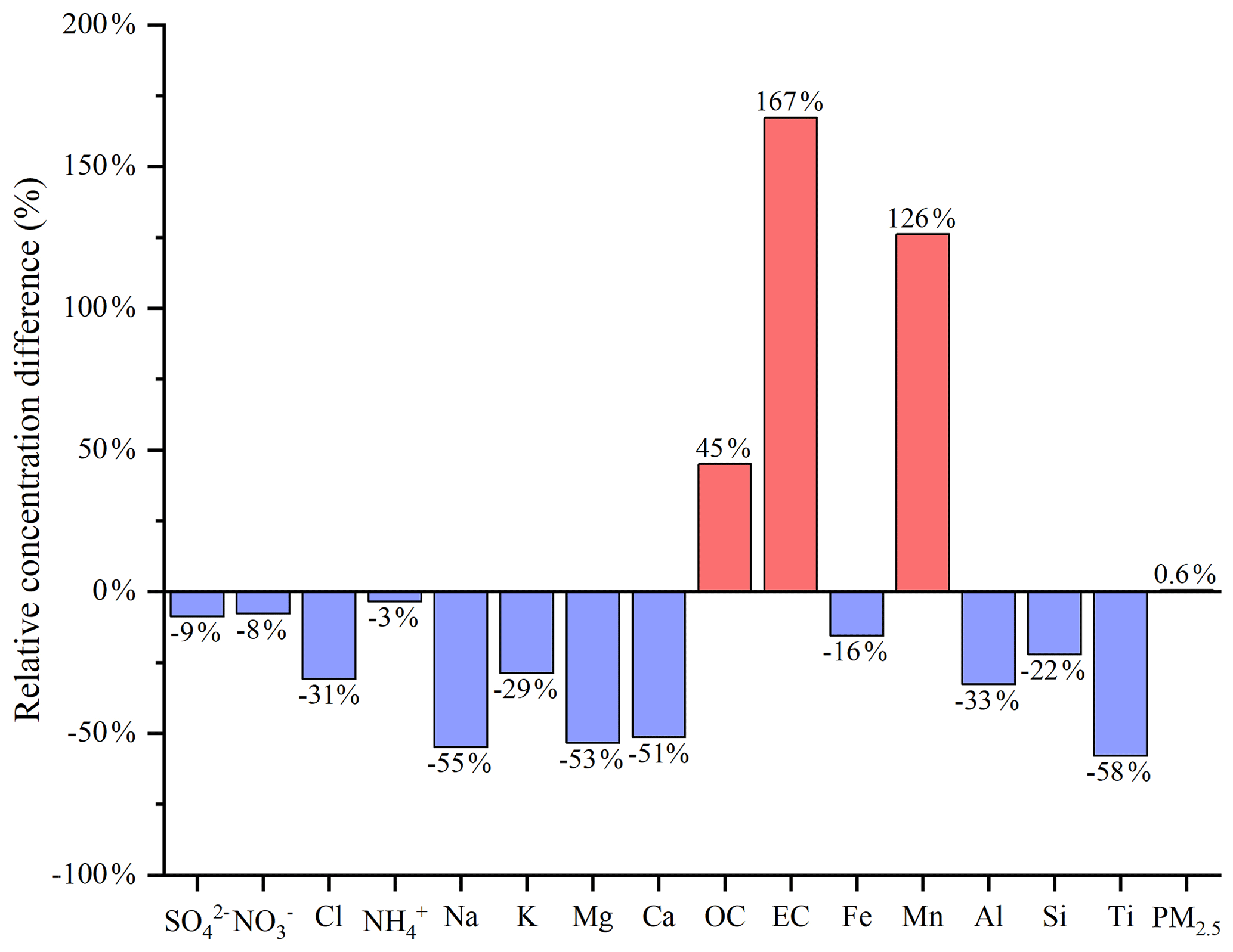
Figure 3 The relative concentration difference in average simulated results (PM_2.5 and its components) between CMAQ_SPE and CMAQ_SPA (relative to CMAQ_SPA) during the simulation period; PM_2.5 source profiles from the SPAPPC and SPECIATE databases were used to create speciated emission inventories for CMAQ, corresponding to cases CMAQ_SPA and CMAQ_SPE, respectively.

4 How large is the impact?

To quantitatively characterize how much the source profiles affect the simulation results, we selected the chemical composition of code 000002.5 (variety of different categories used for the overall average composite profiles; Hsu et al., 2019) in the US EPA SPECIATE_5.0_0 database for species allocation of PM_2.5 components. The corresponding percentages of EC, OC, Mn, Fe, Ti, Al, Si, Ca, Mg, K, Na, Cl, NH${}_{\mathrm{4}}^{+}$, NO${}_{\mathrm{3}}^{-}$ and SO${}_{\mathrm{4}}^{\mathrm{2}-}$ in PM_2.5 are shown in Fig. 4 (SGL, base case simulation).

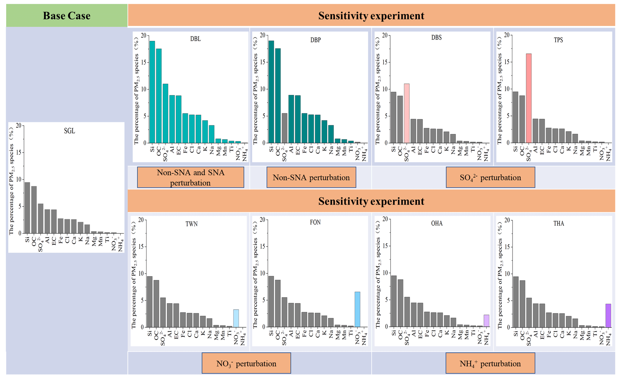
Figure 4 The general roadmap of sensitivity tests (the histogram in each case is the speciation profile in CTMs; SNA represents SO${}_{\mathrm{4}}^{\mathrm{2}-}$, NO${}_{\mathrm{3}}^{-}$ and NH${}_{\mathrm{4}}^{+}$; non-SNA represents other components in PM_2.5).

Table 1 The content of sensitivity experiment cases.

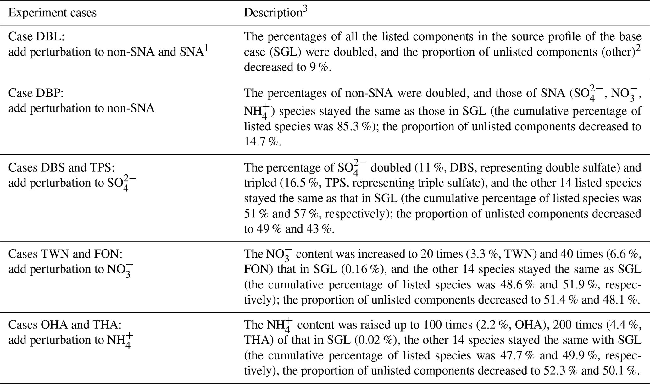
¹ SNA represents SO${}_{\mathrm{4}}^{\mathrm{2}-}$, NO${}_{\mathrm{3}}^{-}$ and NH${}_{\mathrm{4}}^{+}$; non-SNA represents the other components in PM_2.5. ² The listed components contained Al, Ca, Cl, EC, Fe, K, Mg, Mn, Na, OC, Si, Ti, NH${}_{\mathrm{4}}^{+}$, NO${}_{\mathrm{3}}^{-}$ and SO${}_{\mathrm{4}}^{\mathrm{2}-}$; unlisted components were classified as other. ³ The source profiles in all cases listed in the table were calculated based on the base case SGL. In the design of simulation cases, the reason why the disturbance amplitude of NH${}_{\mathrm{4}}^{+}$ and NO${}_{\mathrm{3}}^{-}$ was significantly higher than that of other components such as SO${}_{\mathrm{4}}^{\mathrm{2}-}$ and non-SNA was that the percentages of NH${}_{\mathrm{4}}^{+}$ and NO${}_{\mathrm{3}}^{-}$ in the base source profile (SGL, based on the chemical composition of code 000002.5 in the EPA SPECIATE_5.0_0 database) were very low, while the percentages of NH${}_{\mathrm{4}}^{+}$ and NO${}_{\mathrm{3}}^{-}$ in SPAPPC presented in Sect. 2.2 were orders of magnitude higher than those in SGL.

Given the large quantity and complex chemical composition of PM_2.5, it was advisable to classify the chemical composition reasonably before designing sensitivity experiments. The DBL case consisted of doubling the percentage of the 15 components mentioned in the above base case (SGL) (details are shown in Fig. 4 and Table 1). As the percentage of these components increased, the proportion of unlisted components (represented by other) decreased to 9 % in order to meet the requirement that the total percentage of all components is 100 %. Then we compared the simulation results before (SGL case) and after (DBL case) perturbation in the species allocation of PM_2.5 sources.

In the case of DBL, when the percentages of all the components except those in the other category were doubled in the source profile, the simulated concentrations of Al, Ca, Cl, EC, Fe, K, Mg, Mn, Na, OC, Si and Ti doubled as well, while the simulated concentration of NO₃ and SO${}_{\mathrm{4}}^{\mathrm{2}-}$ increased at about 3 % and 10 % and NH${}_{\mathrm{4}}^{+}$ decreased by 4 %, respectively, although the simulated concentration of PM_2.5 was not obviously changed (detailed simulation results are shown in Table S14). The simulation test results for SNA (SO${}_{\mathrm{4}}^{\mathrm{2}-}$, NO${}_{\mathrm{3}}^{-}$ and NH${}_{\mathrm{4}}^{+}$) and non-SNA were obviously different. Therefore, we divided the components in the source profile into two groups (non-SNA and SNA) and designed a series of sensitivity tests listed in the next section to further explore how species allocation of PM_2.5 in emission sources affects the simulation results. A sketch of the sensitivity experiment design idea is shown in Fig. S7.

4.1 Sensitivity tests design

Sensitivity tests were designed by changing the percentages of the target components and related components in the base case (SGL): add the perturbation to each component of non-SNA, to SO${}_{\mathrm{4}}^{\mathrm{2}-}$, to NO${}_{\mathrm{3}}^{-}$ and to NH${}_{\mathrm{4}}^{+}$. A general roadmap of sensitivity tests is shown in Fig. 4, and an illustration of each case is summarized in Table 1. Basic rules must be followed: (a) the perturbation in the percentage of each component in the source profile falls within the variation range of its measured value described in Sect. 2.2. (b) The sum of the percentage of listed non-SNA, SNA and other components in the PM_2.5 source profile is 100 %.

4.2 Sensitivity of simulated components to changes in the source profile

We propose the sensitivity coefficient (δ) as an evaluation index. The calculation formula is as follows:

$$\begin{array}{}\text{(2)}& \begin{array}{rl}{\mathit{\delta }}_{i,p}& ={\displaystyle \frac{\frac{C_{i\mathit{\_}\mathrm{case}}}{C_{{\mathrm{PM}}_{\mathrm{2.5}}\mathrm{\_}\mathrm{case}}}\times \mathrm{100}\mathit{\%}-\frac{C_{i\mathit{\_}\mathrm{base}}}{C_{{\mathrm{PM}}_{\mathrm{2.5}}\mathrm{\_}\mathrm{base}}}\times \mathrm{100}\mathit{\%}}{P_{p\mathit{\_}\mathrm{case}}-P_{p\mathit{\_}\mathrm{base}}}}\\ & (\text{for DBL and DBP},p=i;\text{for other cases},p=j),\end{array}\end{array}$$

wherein δ_i,p is the sensitivity coefficient of component i relative to component p, representing the change in the simulated value of its content in ambient PM_2.5 corresponding to 1 % perturbation in the source profiles. C_{i_case} is the simulated concentration of component i in each sensitivity experiment case (µg m⁻³), C_{i_base} is the simulated concentration of components i in the base case (µg m⁻³), $C_{{{\mathrm{PM}}_{\mathrm{2.5}}}_{\mathrm{\_}\mathrm{case}}}$ is the simulated concentration of PM_2.5 in each sensitivity experiment case (µg m⁻³), $C_{{{\mathrm{PM}}_{\mathrm{2.5}}}_{\mathrm{\_}\mathrm{base}}}$ is the simulated concentration of PM_2.5 in the base case (µg m⁻³), P_{p_case} is the percentage of component p in the source profile of the sensitivity experiment case (%), j is the perturbed component j in different source profiles of sensitivity experiment cases and P_{p_base} is the percentage of component p in the source profile of the base case (%).

A positive value of δ means the simulated concentration of the PM_2.5 component increases (decreases) with the increase (decrease) in perturbation in the percentage of components in the source profile, and negative δ is just the opposite. If the absolute value of δ is less than or equal to 0.1, the simulated component is considered to be insensitive to the corresponding variation in the source profile; if the absolute value of δ falls between 0.1 and 0.4 (included), the simulated component is considered to be sensitive to the variation in the source profile; if the absolute value of δ is larger than 0.4, the simulated component is very sensitive to the variation in the source profile. The greater the absolute value of δ, the more obvious the impact of the variation in the source profile adopted in CMAQ on the simulated results of PM_2.5 chemical components.

Figure 5 lists the sensitivity coefficients of simulated ambient PM_2.5 components according to the perturbation of the source profile under each test case. In the DBL case (double the percentage of the listed components in the source profile of the base case and decrease the proportion of other unlisted components to 9 %), the sensitivity coefficient (δ) of NH${}_{\mathrm{4}}^{+}$ was negative and the absolute value was high, indicating that the simulated proportion of NH${}_{\mathrm{4}}^{+}$ in ambient PM_2.5 decreased and it was very sensitive to the variation in the source profile. Conversely, the sensitivity coefficient of NO${}_{\mathrm{3}}^{-}$ was close to 1, which illustrated that the simulated proportion of NO${}_{\mathrm{3}}^{-}$ in ambient PM_2.5 increased proportionally with the change in source profile. The simulated SO${}_{\mathrm{4}}^{\mathrm{2}-}$ also showed a very sensitive property. The simulated non-SNA concentrations were doubled when compared to the base case (SGL).

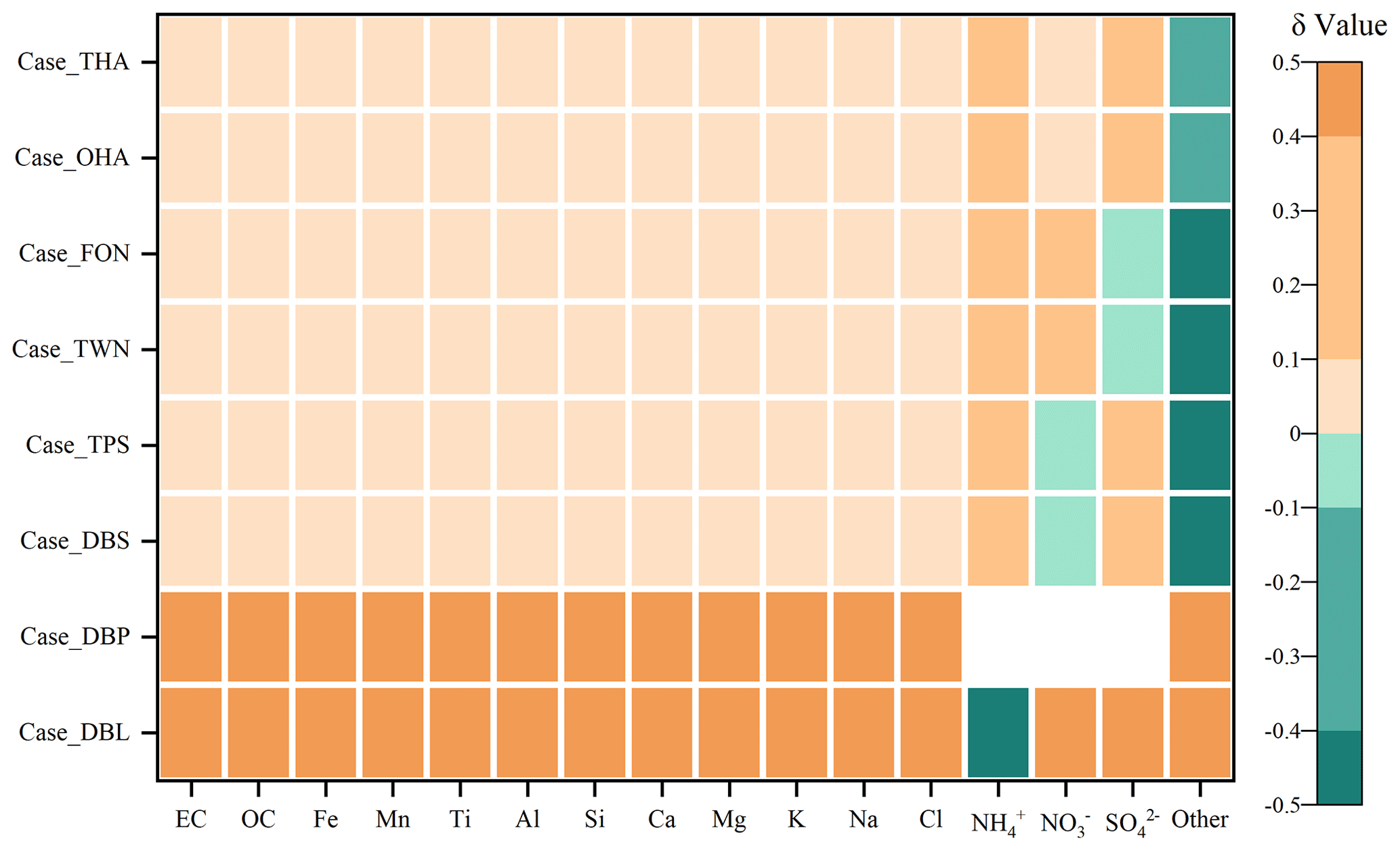
Figure 5 The sensitivity coefficients (δ) of simulated components according to the perturbation of the adopted source profile in different cases. Note: each small color box in the figure represents the sensitivity level (indicated by the legend on the right) of PM_2.5 components (x coordinate) in different cases (y coordinate). The blank grids in the DBP case indicate no perturbation to SNA in the PM_2.5 source profile.

In case DBP, when the percentages of listed non-SNA (Al, Ca, Cl, EC, Fe, K, Mg, Mn, Na, OC, Si and Ti) in the source profile were doubled, the simulated proportions of non-SNA in ambient PM_2.5 synchronous increased and were very sensitive to the change in the adopted source profile, with a sensitivity coefficient (δ) of 0.5. Interestingly, the simulated concentration of SNA in ambient PM_2.5 also changed although SNA in the source profile did not change; the concentration of NO${}_{\mathrm{3}}^{-}$ and SO${}_{\mathrm{4}}^{\mathrm{2}-}$ increased by 2 % and 3 %, respectively, and NH${}_{\mathrm{4}}^{+}$ decreased by 10 % (detailed simulation results of each case are shown in Tables S15–S21).

Under SO${}_{\mathrm{4}}^{\mathrm{2}-}$ perturbation cases (Case DBS and Case TPS), we found the simulated results of non-SNA and NO${}_{\mathrm{3}}^{-}$ had no obvious variation compared with the base case. In both Case DBS and Case TPS, the δ values of non-SNA and NO${}_{\mathrm{3}}^{-}$ were between −0.1 and 0.1. But when the percentage of SO${}_{\mathrm{4}}^{\mathrm{2}-}$ was doubled in source profile (DBS), the simulated concentration of NH${}_{\mathrm{4}}^{+}$ and SO${}_{\mathrm{4}}^{\mathrm{2}-}$ increased by 6 % and 8 %, respectively. In Case TPS (the percentage of SO${}_{\mathrm{4}}^{\mathrm{2}-}$ was tripled), the simulated concentrations of NH${}_{\mathrm{4}}^{+}$ and SO${}_{\mathrm{4}}^{\mathrm{2}-}$ were increased by 11 % and 16 %, respectively. The δ values of NH${}_{\mathrm{4}}^{+}$ and SO${}_{\mathrm{4}}^{\mathrm{2}-}$ were 0.12 and 0.36, sensitive toward the positive direction with the increase in SO${}_{\mathrm{4}}^{\mathrm{2}-}$ in the source profile.

In the situation of NO${}_{\mathrm{3}}^{-}$ perturbation in the source profile (Case TWN and Case FON), the simulated non-SNA hardly changes when compared to the base case, while changing patterns of simulated SNA were different. The simulation concentration of NH${}_{\mathrm{4}}^{+}$ increased by 2.6 % and 5.4 % compared with the base case, the simulated NO${}_{\mathrm{3}}^{-}$ increased by 14 % and 30 %, and the simulated SO${}_{\mathrm{4}}^{\mathrm{2}-}$ decreased slightly and even could be neglected in some observation sites. The simulated concentrations of non-SNA and SO${}_{\mathrm{4}}^{\mathrm{2}-}$ were insensitive to the perturbation of NO${}_{\mathrm{3}}^{-}$ in the source profile; NH${}_{\mathrm{4}}^{+}$ was sensitive, and NO${}_{\mathrm{3}}^{-}$ was very sensitive.

When we add perturbation to NH${}_{\mathrm{4}}^{+}$ in the source profile (Case OHA and Case THA), the simulation results of non-SNA were almost not changed, whereas the simulated concentration of SO${}_{\mathrm{4}}^{\mathrm{2}-}$, NH${}_{\mathrm{4}}^{+}$ and NO${}_{\mathrm{3}}^{-}$ increased. The δ values of SNA in response to the variation in NH${}_{\mathrm{4}}^{+}$ in the source profile were positive, and ${\mathit{\delta }}_{{\mathrm{SO}}_{\mathrm{4}}^{\mathrm{2}-},{\mathrm{NH}}_{\mathrm{4}}^{+}}$ > ${\mathit{\delta }}_{{\mathrm{NH}}_{\mathrm{4}}^{+},{\mathrm{NH}}_{\mathrm{4}}^{+}}$ > ${\mathit{\delta }}_{{\mathrm{NO}}_{\mathrm{3}}^{-},{\mathrm{NH}}_{\mathrm{4}}^{+}}$; SO${}_{\mathrm{4}}^{\mathrm{2}-}$ and NH${}_{\mathrm{4}}^{+}$ were sensitive to the NH${}_{\mathrm{4}}^{+}$ perturbation in the source profile, but NO${}_{\mathrm{3}}^{-}$ was not so sensitive.

In general, the simulation results of components in ambient PM_2.5 were affected in one way or another by the change in source profiles adopted by CMAQ. Both of the simulated non-SNA and the simulated SNA were very sensitive to the perturbation of non-SNA in the source profile. When the percentage of SNA changed in the source profile, simulated non-SNA generally changed little, but the simulation results of SNA could change in different patterns: the simulated SO${}_{\mathrm{4}}^{\mathrm{2}-}$ was very sensitive and NH${}_{\mathrm{4}}^{+}$ was sensitive to the perturbation of SO${}_{\mathrm{4}}^{\mathrm{2}-}$ in the source profile; simulated NO${}_{\mathrm{3}}^{-}$ was very sensitive and NH${}_{\mathrm{4}}^{+}$ was sensitive to the perturbation of NO${}_{\mathrm{3}}^{-}$ in the source profile; SO${}_{\mathrm{4}}^{\mathrm{2}-}$ and NH${}_{\mathrm{4}}^{+}$ were sensitive to the perturbation of NH${}_{\mathrm{4}}^{+}$ in the source profile. The simulated component such as SO${}_{\mathrm{4}}^{\mathrm{2}-}$ was influenced not only by the change in SO${}_{\mathrm{4}}^{\mathrm{2}-}$ itself but also by other components like some non-SNA and NH${}_{\mathrm{4}}^{+}$ in the source profile. In other words, there was a linkage effect, variation in some components in the source profile would bring changes to the simulated results of other components.

5 How does the impact work?

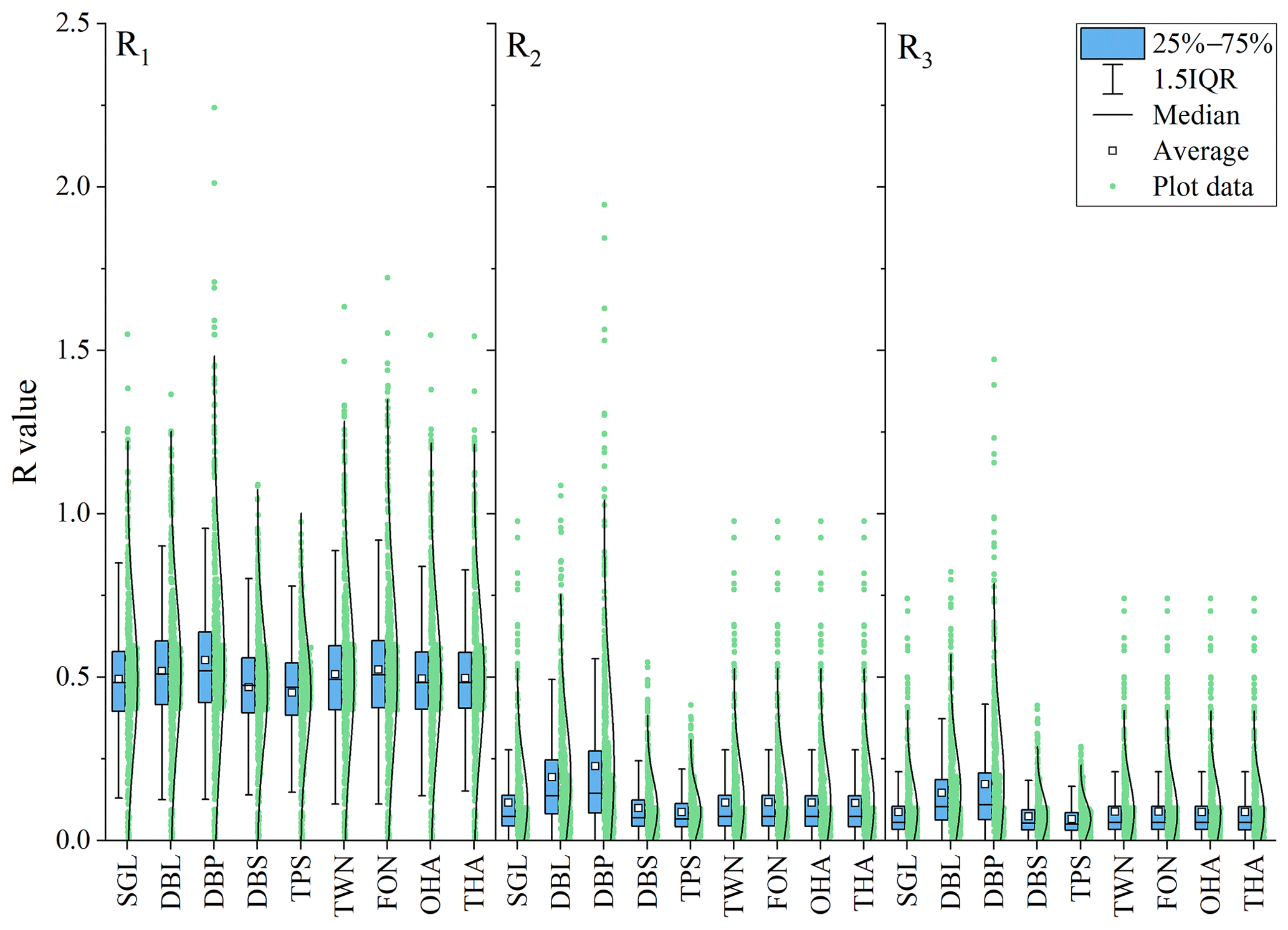
The variation in species allocation in emission sources can directly affect the composition of aerosol systems in CTMs. In CMAQv5.0.2, the aerosol thermodynamic equilibrium process is carried out according to ISORROPIA II, including a SO${}_{\mathrm{4}}^{\mathrm{2}-}$–NO${}_{\mathrm{3}}^{-}$–Cl⁻–NH${}_{\mathrm{4}}^{+}$–Na⁺–K⁺–Mg²⁺–Ca²⁺–H₂O system (detailed equilibrium relations are shown in Table S22). Some assumptions have been made in the ISORROPIA model to simplify the simulation system (Fountoukis and Nenes, 2007): (1) because the vapor pressure of sulfuric acid and metal salts (such as Na⁺, Ca²⁺, K⁺, Mg²⁺) is very low, it is assumed that all the sulfuric acid and metal salts in the system existed in the aerosol phase; (2) for ammonia in the system, it is preferred to have an irreversible reaction with sulfuric acid to produce ammonium sulfate. Only when there is still surplus NH₃ after the neutralization of H₂SO₄ can it have a reversible reaction with HNO₃ and HCl to produce NH₄NO₃ and NH₄Cl. (3) For sulfuric acid in the system, if there are metal ions (such as Ca²⁺, Mg²⁺, K⁺, Na⁺) in the system, sulfuric acid would react with metal ions to produce metal salts. Only in the case of insufficient sodium would sulfuric acid react with ammonia. Based on these assumptions, the ISORROPIA model introduces the following three judgment parameters (R₁, R₂ and R₃) to determine the simulation subsystems; these parameters are calculated by the following formulas:

$$\begin{array}{}\text{(3)}& {\displaystyle }{R}_{\mathrm{1}}={\displaystyle \frac{\left[{\mathrm{NH}}_{\mathrm{4}}^{+}\right]+\left[{\mathrm{Ca}}^{\mathrm{2}+}\right]+\left[{\mathrm{K}}^{+}\right]+\left[{\mathrm{Mg}}^{\mathrm{2}+}\right]+\left[{\mathrm{Na}}^{+}\right]}{\left[{\mathrm{SO}}_{\mathrm{4}}^{\mathrm{2}-}\right]}},\text{(4)}& {\displaystyle }{R}_{\mathrm{2}}={\displaystyle \frac{\left[{\mathrm{Ca}}^{\mathrm{2}+}\right]+\left[{\mathrm{K}}^{+}\right]+\left[{\mathrm{Mg}}^{\mathrm{2}+}\right]+\left[{\mathrm{Na}}^{+}\right]}{\left[{\mathrm{SO}}_{\mathrm{4}}^{\mathrm{2}-}\right]}},\text{(5)}& {\displaystyle }{R}_{\mathrm{3}}={\displaystyle \frac{\left[{\mathrm{Ca}}^{\mathrm{2}+}\right]+\left[{\mathrm{K}}^{+}\right]+\left[{\mathrm{Mg}}^{\mathrm{2}+}\right]}{\left[{\mathrm{SO}}_{\mathrm{4}}^{\mathrm{2}-}\right]}},\end{array}$$

where [X] denotes the molar concentration of the component (mol m⁻³) and R₁, R₂ and R₃ are termed as the “total sulfate ratio”, “crustal species and sodium ratio” and “crustal species ratio”, respectively. The numbers of species and equilibrium reactions are determined by the relative abundance of NH₃, Na, Ca, K, Mg, HNO₃, HCl and H₂SO₄, as well as the ambient relative humidity and temperature. Guided by the values of R₁, R₂ and R₃, five aerosol composition regimes in ISORROPIA are defined. (Detailed rules are shown in Table S27 and the solving procedure in Fig. S8.) R₁, R₂ and R₃ in each sensitivity test case are shown in Fig. 6. These components achieved thermodynamic equilibrium in the order of preference for more stable salts; obviously, the simulation processes of these components may influence each other.

5.1 General results

Our sensitivity experiment focuses on examining the impact of source profile changes on simulated PM_2.5 components. For given meteorological conditions, we analyze the sensitivity of simulated components to variations in the source chemical profile by comparing the simulation results between perturbed cases and the base case.

Figure 6 R values' distribution among the base case and different sensitivity test cases.

In the non-SNA perturbation case, when the percentage of non-SNA in the source profile was doubled (Case DBP), there were more Na, K, Mg, Ca and Cl participating in the aerosol chemistry; the model system needed more SO${}_{\mathrm{4}}^{\mathrm{2}-}$ and NO${}_{\mathrm{3}}^{-}$ on the basis of charge balance; and the thermodynamic equilibrium shifted to the direction of consuming Ca, Mg, K and Na, which resulted in the increase in the simulated concentration of SO${}_{\mathrm{4}}^{\mathrm{2}-}$ and NO${}_{\mathrm{3}}^{-}$. Meanwhile, according to the rule of anions preferentially binding with nonvolatile cations in ISORROPIA, the increased cations of Na⁺, K⁺, Mg²⁺ and Ca²⁺ directly led to the decrease in anions binding with NH${}_{\mathrm{4}}^{+}$; there was less reaction dose between SO${}_{\mathrm{4}}^{\mathrm{2}-}$ and NH${}_{\mathrm{4}}^{+}$ to form (NH₄)₂SO₄ or NH₄HSO₄, ultimately resulting in a decrease in the simulated concentration of NH${}_{\mathrm{4}}^{+}$ compared with the base case. Because in this case more anions such as SO${}_{\mathrm{4}}^{\mathrm{2}-}$ were passively needed, according to the principle of chemical equilibrium mentioned above, the chemical conversion of SO₂ to SO${}_{\mathrm{4}}^{\mathrm{2}-}$ was promoted and the simulated secondary SO${}_{\mathrm{4}}^{\mathrm{2}-}$ increased; this could be proved by the sensitivity coefficient δ of SO₂ in Case DBP being negative (shown in Fig. 7; details of other monitoring stations' results are shown in Table S25).

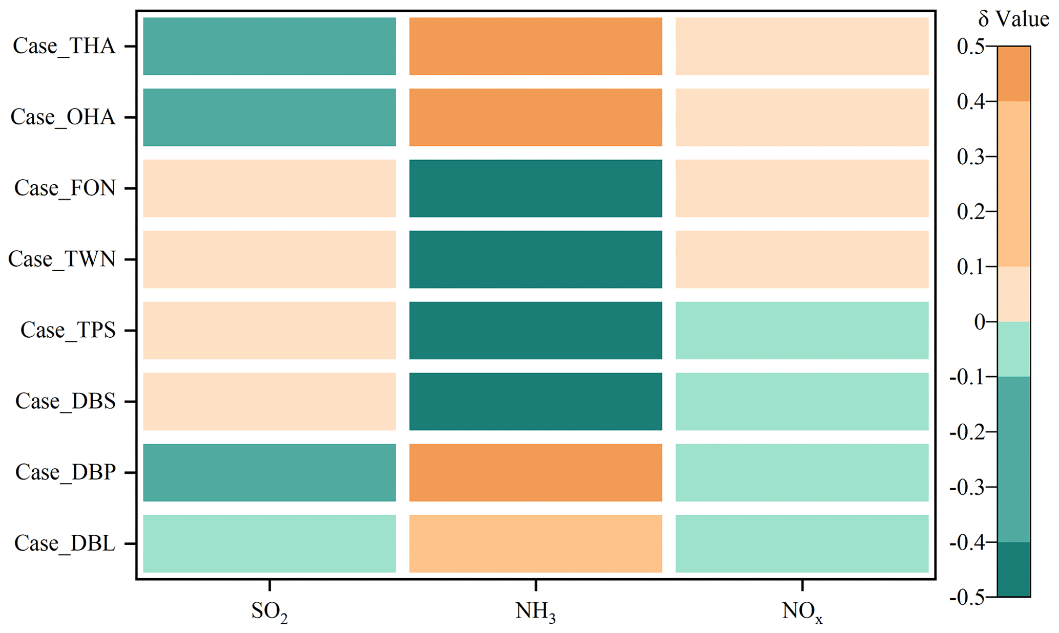
Figure 7 The sensitivity coefficients (δ) of simulated gas pollutants according to the change in the adopted source profile in different cases.

Similarly, with the increase in metal ions in the system to bond with anions, the number of anions which can bind to NH${}_{\mathrm{4}}^{+}$ decreased. The system needed less NH${}_{\mathrm{4}}^{+}$, and the need for conversion from NH₃ to NH${}_{\mathrm{4}}^{+}$ was weakened; the simulated NH${}_{\mathrm{4}}^{+}$ concentration decreased, while the δ of NH₃ was positive and very sensitive. Different trends of the simulated concentration of gaseous pollutants mirrored the rules mentioned above in terms of another aspect. The δ of SO₂ and NO_x was negative and that of NH₃ was positive. We could see the same phenomena in DBL case (Fig. 7). When the percentages of non-SNA in the source profile increased, they affected not only the simulated concentration of non-SNA, but also the secondary SO${}_{\mathrm{4}}^{\mathrm{2}-}$, NO${}_{\mathrm{3}}^{-}$ and NH${}_{\mathrm{4}}^{+}$.

Figure 8 The sensitivity coefficients (δ) under different hierarchical patterns.

In SO${}_{\mathrm{4}}^{\mathrm{2}-}$ perturbation cases (Case DBS and Case TPS), as the percentage of SO${}_{\mathrm{4}}^{\mathrm{2}-}$ in the source profile increased, for the chemical reactions of sulfate radical consumption (as shown in Table S22), the chemical equilibrium would move toward the products compared with the base case. In contrast, for the chemical reactions of sulfate radical formation (the equations are shown in Table S23), the product was added in and the chemical equilibrium was pushed toward the reactants. The chemical reactions between SO${}_{\mathrm{4}}^{\mathrm{2}-}$ and NH${}_{\mathrm{4}}^{+}$ would shift to the direction of (NH₄)₂SO₄ or NH₄HSO₄ generation, and we could see the simulated concentrations of NH${}_{\mathrm{4}}^{+}$ in DBS and TPS were both higher and in NH₃ were lower than those in the base case (SGL). In addition, when more SO${}_{\mathrm{4}}^{\mathrm{2}-}$ was added to the system, the conversion of SO₂ to SO${}_{\mathrm{4}}^{\mathrm{2}-}$ was affected at some level, less SO₂ was consumed than in the base case and simulated SO₂ showed an insensitive but positive trend (Fig. 7). The potential solid-phase species in ISORROPIA II under DBS and TPS cases (shown in Table S27) mainly consisted of sulfate salts, so the simulated concentration of NO${}_{\mathrm{3}}^{-}$ did not change apparently.

As the percentage of NO${}_{\mathrm{3}}^{-}$ in the source profile increased (Case FON and Case TWN), the associated chemical equilibrium shifted toward the consumption of NO${}_{\mathrm{3}}^{-}$, such as NH${}_{\mathrm{4}}^{+}+$ NO${}_{\mathrm{3}}^{-}$ → NH₄NO₃, which would also result in the consumption of more NH${}_{\mathrm{4}}^{+}$ and formation of more ammonium salt and finally the consumption of more NH₃ because of NH₃(gas) + H₂O(aq) → NH${}_{\mathrm{4}}^{+}$(aq) + OH⁻(aq). The simulation results also showed that the concentration of NH${}_{\mathrm{4}}^{+}$ increased while that of NH₃ decreased. Based on the assumption of ISORROPIA, the cations like Na⁺, K⁺, Mg²⁺, Ca²⁺ and NH${}_{\mathrm{4}}^{+}$ preferentially react with SO${}_{\mathrm{4}}^{\mathrm{2}-}$; only if there are cations left after neutralized SO${}_{\mathrm{4}}^{\mathrm{2}-}$ can they react with NO${}_{\mathrm{3}}^{-}$ to form salts, so the simulated concentration of SO${}_{\mathrm{4}}^{\mathrm{2}-}$ was not obviously changed. Accordingly, the simulated concentration of NO_x and SO₂ was almost unchanged (the δ of NO_x and SO₂ was insensitive).

In the cases of NH${}_{\mathrm{4}}^{+}$ perturbation (Case OHA and Case THA), when the percentage of NH${}_{\mathrm{4}}^{+}$ in the source profile increased, the related chemical equilibrium shifted toward the direction of NH${}_{\mathrm{4}}^{+}$ consumption, such as in 2NH${}_{\mathrm{4}}^{+}$ + SO${}_{\mathrm{4}}^{\mathrm{2}-}$ → (NH₄)₂SO₄ or NH${}_{\mathrm{4}}^{+}$ + H⁺, SO${}_{\mathrm{4}}^{\mathrm{2}-}$ → NH₄HSO₄; more SO${}_{\mathrm{4}}^{\mathrm{2}-}$ was consumed at the same time, which further promoted the conversion of SO₂ to SO${}_{\mathrm{4}}^{\mathrm{2}-}$. The increased NH${}_{\mathrm{4}}^{+}$ in OHA and THA would also inhibit the conversion of NH₃ to NH${}_{\mathrm{4}}^{+}$ compared with the base case. This, in turn, appeared as an increase in the simulated secondary SO${}_{\mathrm{4}}^{\mathrm{2}-}$ and NH₃ and a decrease in the simulated SO₂.

5.2 Results from stratified analysis

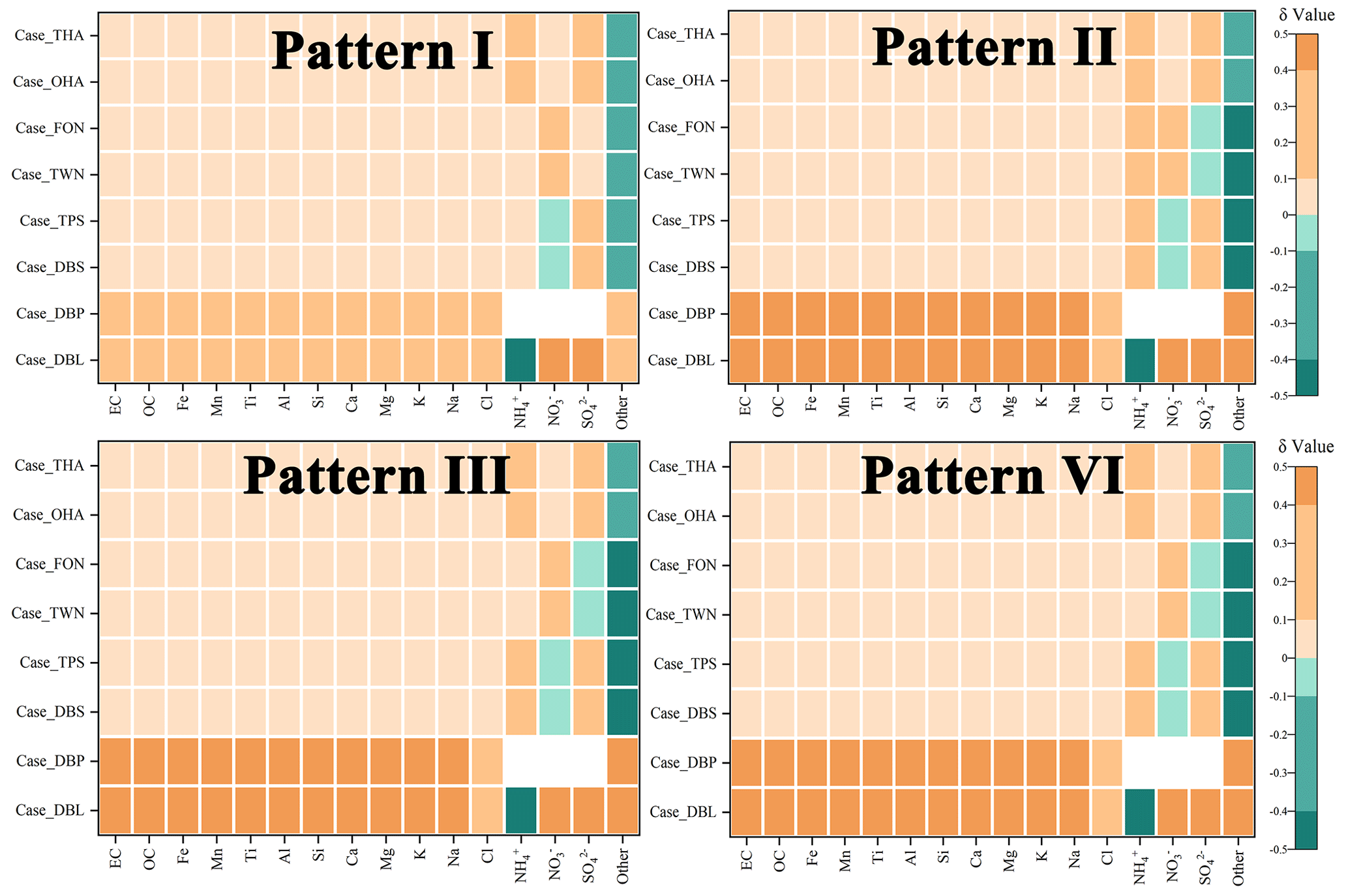
For each case, the distribution of R values was related to meteorological conditions (as shown in Fig. 6). To illustrate the role of meteorological conditions in the mechanism of how the source profile affected the simulated PM_2.5 components, stratified analysis was used. The hourly simulation result of temperature and humidity (affecting the ISORROPIA solving procedure) and the wind field (affecting flux in and flux out for each grid) were incorporate into k-means clustering. When the number of clusters was equal to or greater than four, there was a significant inflection point between data points and their assigned cluster centroids (Fig. S9). Hence, four patterns of meteorological conditions were selected for the subsequent analysis.

For patterns I, II, III and IV, as shown in Fig. 8, the rule similar to the general result was observed. From a global view, the subdivisional (category-specific) sensitivity of simulated PM_2.5 components to the source chemical profile under different patterns is similar; from a local perspective, their sensitivity levels are slightly different. For example, in pattern II, the simulated NH${}_{\mathrm{4}}^{+}$ was very sensitive to the perturbation of SO${}_{\mathrm{4}}^{\mathrm{2}-}$, while in patterns I, III and VI it was sensitive, but it remained the major component that underwent change (these results are also shown in Table S28 of the Supplement).

When we perturb the source profile, some species/reactants increase (or decrease) in the system and the chemical equilibrium shift to the direction of consuming more (or fewer) reactants, as shown in Fig. S10. According to different patterns of meteorological conditions (determining the values of R), the influence pathways of chemical source profile changes on the simulated PM_2.5 components has the same laws as the general results.

In summary, the effects of source profile variation on the simulation results of different components were linked. When the percentages of non-SNA, SO${}_{\mathrm{4}}^{\mathrm{2}-}$, NO${}_{\mathrm{3}}^{-}$ and NH${}_{\mathrm{4}}^{+}$ in the source profile changed, they not only affected the simulated concentration of themselves, but also affected the simulation results of some other components. The simulation results of both primary components and secondary components were affected by the change in the source profile; the secondary SO${}_{\mathrm{4}}^{\mathrm{2}-}$ and NH${}_{\mathrm{4}}^{+}$ were affected more than the secondary NO${}_{\mathrm{3}}^{-}$.

6 Conclusions

The influence of source profile variation on the simulated PM_2.5 components cannot be ignored, as simulation results of some components are sensitive to the adopted source profile in CTMs; e.g., both the simulated non-SNA and the simulated SNA are sensitive to the perturbation of non-SNA in the source profile, the simulated SO${}_{\mathrm{4}}^{\mathrm{2}-}$ and NH${}_{\mathrm{4}}^{+}$ are sensitive to the perturbation of SO${}_{\mathrm{4}}^{\mathrm{2}-}$, the simulated NO${}_{\mathrm{3}}^{-}$ and NH${}_{\mathrm{4}}^{+}$ are sensitive to the perturbation of NO${}_{\mathrm{3}}^{-}$, and SO${}_{\mathrm{4}}^{\mathrm{2}-}$ and NH${}_{\mathrm{4}}^{+}$ are sensitive to the perturbation of NH${}_{\mathrm{4}}^{+}$. These influences not only are specific to an individual component, but also can be transmitted and linked between components. The influence path is connected to chemical mechanisms in the model, since the variation in species allocation in emission sources directly affects the thermodynamic equilibrium system (ISORROPIA II, SO${}_{\mathrm{4}}^{\mathrm{2}-}$–NO${}_{\mathrm{3}}^{-}$–Cl⁻–NH${}_{\mathrm{4}}^{+}$–Na⁺–K⁺–Mg²⁺–Ca²⁺–H₂O system).

It is generally believed that changes in the source profile would have an impact on the simulation result of primary PM_2.5, but interestingly, the simulation of secondary components could be affected as well. We found the perturbation of the PM_2.5 source profile caused the variation in simulation results of gaseous pollutants by influencing related chemical reactions like gas-phase chemistry of SO₂, NO_x and NH₃. Overall, the emission source profile used in CTMs is one of the important factors affecting the simulation results of PM_2.5 chemical components. Additionally, organic species are one of the most important components in PM_2.5 and gain much attention in relation to human health. While the number of organic species in the source profile is relatively low, which brings a challenge for simulation test designing, the influence of the source profile on the simulation results of organic species is not taken into account in this study.

With changes in fuel and raw materials, the development of production technology, and the innovation of pollution treatment technology in recent years, some components have changed significantly in source profiles. Given the important role of air quality simulation in decision-making for pollution control and health risk assessment, the representativeness and timeliness of the source profile should be considered.

Our study tentatively discussed the influence of mechanisms of PM_2.5 emission source profiles on the simulation results of components in CTMs. The size distribution, mixing state, aging and solubility for different aerosol components might have something to do with source profile; the extent of the influence of source profile changes on the simulation of these physical and chemical process deserves future study.