the Creative Commons Attribution 4.0 License.
the Creative Commons Attribution 4.0 License.
 | 21 Nov 2023
Modelling detrital cosmogenic nuclide concentrations during landscape evolution in Cidre v2.0
Sébastien Carretier
Vincent Regard
Youssouf Abdelhafiz
Bastien Plazolles
The measurement of cosmogenic nuclide (CN) concentrations in riverine sediment has provided breakthroughs in our understanding of landscape evolution. Yet, linking this detrital CN signal and relief evolution is based on hypotheses that are not easy to verify in the field. Models can be used to explore the statistics of CN concentrations in sediment grains. In this work, we present a coupling between the landscape evolution model Cidre and a model of the CN concentration in distinct grains. These grains are exhumed and detached from the bedrock and then transported in the sediment to the catchment outlet with temporary burials and travel according to the erosion–deposition rates calculated spatially in Cidre. The concentrations of various CNs can be tracked in these grains. Because the CN concentrations are calculated in a limited number of grains, they provide an approximation of the whole CN flux. Therefore, this approach is limited by the number of grains that can be handled in a reasonable computing time. Conversely, it becomes possible to record part of the variability in the erosion–deposition processes by tracking the CN concentrations in distinct grains using a Lagrangian approach. We illustrate the robustness and limitations of this approach by deriving the catchment-average erosion rates from the mean 10Be concentration of grains leaving a synthetic catchment and comparing them with the erosion rates calculated from sediment flux, for different uplift scenarios. We show that the catchment-average erosion rates are approximated to within 5 % uncertainty in most of the cases with a limited number of grains.
- Article
(3724 KB) - Full-text XML
- BibTeX
- EndNote


The concentration of cosmogenic nuclides (CN) produced in situ varies according to the depth of the minerals in which they are produced, their altitude, the stable or radioactive nature of the nuclide in question and the magnetic field (Gosse and Phillips, 2001). When a mineral in a grain is exhumed and then transported in rivers, the concentration of CN evolves by integrating stochastic variations of the residence times at different depths and altitudes over time. This integrative characteristic has been used to develop numerous approaches to quantify erosion–deposition processes averaged over catchment areas and millennia (Schaefer et al., 2022). The most widespread approach is one that quantifies the average erosion rate of a catchment from its average CN concentration in a sand sample taken at its outlet (Brown et al., 1995). Since the pioneering work of Repka et al. (1997), other studies have explored the possibility of using the distribution of CN concentrations in distinct grains and possibly grains of different sizes to quantify erosion–deposition processes on hillslopes, in rivers and on alluvial deposits over periods of several thousand to millions of years (Braucher et al., 1998; Dunai et al., 2005; Gayer et al., 2008; Codilean et al., 2008; Carretier et al., 2019). However, it is still difficult to link detrital CN concentration data to specific processes, whether on hillslopes or on a larger scale in river systems (Yanites et al., 2009). This difficulty arises from the stochasticity of grain transport, which can be temporarily stored and then recycled on different scales ranging from a flood event that erodes the banks of an alluvial river to millions of years in the case of exhumation of ancient strata of a foreland basin.
To address this complexity, several models have been developed at the grain and catchment scales (Repka et al., 1997; Niemi et al., 2005; Codilean et al., 2008; Carretier et al., 2009, 2019; Ben-Israel et al., 2022), but without taking the evolution of the relief, and thus of the CN production rate, into account. At the same time, landscape evolution models (LEMs) have made great progress by integrating an increasing number of processes; however, their resolution over long time spans limits taking into account stochastic phenomena that require the intermittent storage of sediment grains on hillslopes (e.g. landslides) and along fluvial systems (e.g. sediment bars and terraces). Carretier et al. (2016) proposed a coupling between the landscape evolution model in Cidre and the transport of tracer grains which are transported stochastically according to simple probability laws depending on the local erosion and deposition rates calculated on each cell of the LEM. This allowed those authors to highlight that some grains may have been stored for a long time before being recycled and evacuated by the rivers (Carretier et al., 2020). In this paper, we present a development in Cidre to calculate the concentration of several CNs within the grains. To our knowledge, the only published model that can jointly model the evolution of the relief and the evolution of the average CN concentration in the sediments is Badlands (Petit et al., 2023). In Badlands, this average concentration is calculated in proportion to the sediment fluxes from the different upstream sources on each grid cell. In Cidre, we adopt a different (i.e. Lagrangian) approach, which enables us to track the full distribution of CN concentrations in a population of grains.
We first present the Cidre model, including grain transport, and then describe the equations used to calculate the CN concentration over time in each grain. We show the accuracy and robustness of the algorithm by comparing the average catchment erosion rate derived from the CN concentrations of outgoing grains with the true rate calculated in several simulations. In the following we call the “true” catchment-average erosion rate the ratio of the sediment “outlux” over the catchment area calculated in Cidre. In particular, we show that this true rate is approximated to within 5 % uncertainty in most of the cases with a limited number of grains.
2.1 Mass balance equation
Cidre is a c++ code that solves the following mass balance on rectangular cells expressed here for the mean elevation z of a cell through time t:
This mass balance refers to the erosion (“ϵ”)–deposition (“D”) model (Davy and Lague, 2009) where the subscript “r” (“river”) refers to erosion driven by flowing water and “h” (“hillslope”) to erosion due only to the topographic gradient or slope S. U is a vertical uplift or subsidence rate. Then, we define a constitutive law for each of these components (Carretier et al., 2016):
where K [L1−2 m Tm−1] and κ [L T−1] are erodibility parameters; m and n are lithology-dependent (different for bedrock or sediment) erosion parameters; S is the slope (absolute value of the elevation gradient) towards the downstream cell in the steepest direction; and q [L3 T−1] is the water discharge per stream unit width, corresponding to the accumulation of the net precipitation rate (specified in the input or varying dynamically with elevation; Zavala et al., 2020) from the highest to lowest cell according to a multiple flow algorithm, spreading the water discharge of the cell towards all the lower cells among the eight neighbouring cells proportionally to their slope. There is no erosion in a pit cell, only deposition. The deposition rate is
where qsr and qsh are the incoming river and hillslope sediment fluxes (total ) per unit width [L2 T−1], ζ is a river transport length parameter [T L−1] and Sc is a slope threshold. These fluxes are the sum of the sediment fluxes leaving upstream neighbouring cells while the deposition rates on a cell are a fraction of the incoming sediment. Note that the hillslope equations derive from the non-linear diffusion model (Roering et al., 1999) but are written as an erosion–deposition model. Both formulations lead to the similar topographic evolution, but the model used in Cidre is numerically more stable and more adapted to the coupling with grains transport (Carretier et al., 2016).
Equation (1) is solved using the forward finite volume method (z represents the mean elevation of a cell). At each iteration, cells of the model grid are ranked in a decreasing elevation order and then treated successively in that order to ensure that all incoming water and sediment fluxes are known when treating a given cell. For each cell, incoming water fluxes are summed with the local volume of precipitation falling on a cell over the time step. The resulting water flux is then spread among all the downstream cells in proportion to their local topographic gradient (multiple flow), or slope. Then the eroded flux is first calculated on that cell from Eqs. (2) and (3) using the steepest-descent slope among the downstream neighbouring cells. If the erosion potential (the erosion rate multiplied by the time step) is larger than the sediment volume present on that cell, the bedrock is eroded in proportion to the remaining time step (). Then, the deposition flux is calculated using Eqs. (4) and (5). Erosion–deposition is first calculated for the hillslope processes and then for rivers. Once the total eroded and deposited volumes are known, the elevation is modified based on the balance between these two volumes. Sediments that leave the cell are distributed to downstream cells in proportion to the local slope of neighbouring cells. Then, the next cell in the list is treated and so on. When all the cells have been treated, a new iteration begins and the time is incremented by dt.
Other processes, such as lateral erosion, weathering and regolith development, orographic precipitation or the dynamic filling of depressions, are implemented but not described in this paper because the algorithm to calculate the CN concentrations in the grains does not vary according to these processes (see Carretier et al., 2016, 2018; Zavala et al., 2020).
2.2 The grains in Cidre
Grains are clasts of any kind, for example, a single mineral or a pebble composed of multiple minerals, ranging in size from millimetres to decimetres (Carretier et al., 2016). They are localized by the index corresponding to the cell number where they are located (their precise 2D coordinates within a cell are not known) and the depth of their centre beneath the earth's surface. At the beginning of a simulation, their number, radius R, location on the grid and depth z′ are specified. For example, they can be set randomly on the grid and at depth if the grains are quartz grains and the proportion of quartz is constant in the underlying rock. Alternatively, grains can be set with a higher proportion in some cells or at some depths for which the rock has a higher quartz content.
Grains are moved once the erosion and deposition rates are known on the model grid at the end of a time step. They are passive tracers, they do not influence the erosion and sediment calculated by Cidre and they are all independent from each other. Grains are eroded, transported or deposited according to probabilities depending on the erosion and deposition rates. For a grain on a cell, it is detached if the eroded layer on that time step is thicker than or equal to the depth of the grain's bottom . If the grain is not detached, its depth is updated according to the dz calculated on that cell and for this time step. It is possible for a grain to be detached but to not leave the cell to account for the time needed to travel to a larger cell, and for the slower transport of a big grain. Carretier et al. (2016) found that to account for these effects and to predict the correct mean sediment flux, the probability of leaving a cell should be , where δ=1 if the direction of movement is parallel to rows or columns and along diagonals. (A longer distance decreases the probability of leaving the cell.) The computation is made successively on a cell for hillslopes (ϵ=ϵh) and for river processes (ϵ=ϵr). The value of this probability is set to 1 if it exceeds unity, which may occur if the grain is at the surface and the erosion is larger than the grain diameter. If the grain does not leave the cell, its depth is chosen randomly within the layer deposited on that cell during the time step.
If a grain leaves the cell, it goes to one of the downstream neighbouring cells with a probability set as the ratio of the local slope of the considered downstream cell and the sum of the downstream slopes. Once the grain has entered into one of these downstream cells, the probability that it will be deposited is the ratio of the sediment deposition volume in that cell to the sum of the incoming sediment volumes. If not deposited, the grain continues its travel and is exported towards one of the downstream cells, and so on until it is deposited or leaves the model grid. Then a new grain is treated and so on. When all the grains have been treated, a new time step is initiated to calculate the local erosion and deposition on the model grid.
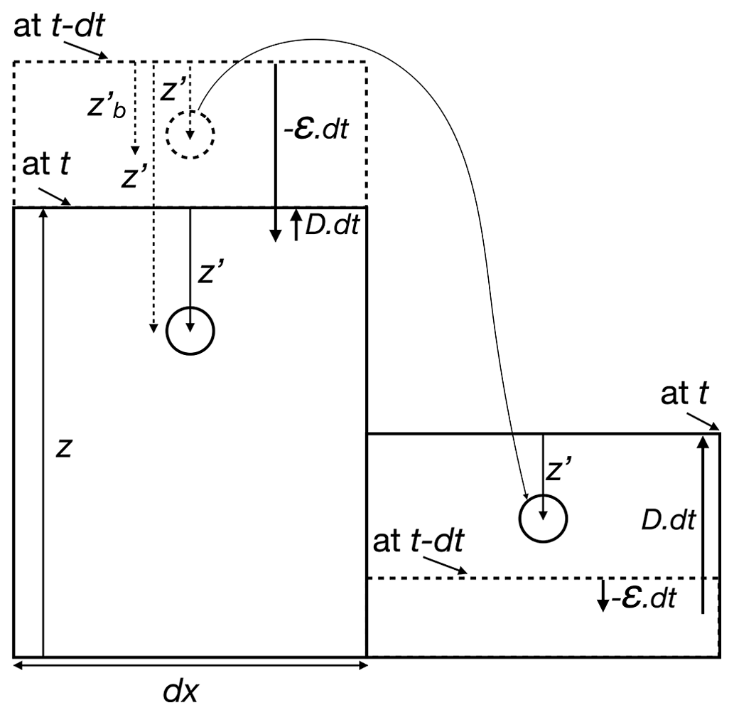
Figure 1 The vertical coordinates of two grains, one staying at depth during a time step and the other moving to a downstream cell where it is deposited. Dashed lines correspond to t−dt and solid lines to t. The upstream cell has a net negative topographic change (erosion) over the time step “dt” (ϵ>D). The downstream cell has a net positive change (sedimentation). The eroded (ϵ⋅dt) and deposited (D ⋅dt) thicknesses are calculated for hillslope and then river processes (see Eqs. 2 and 4). In both cases, a grain is potentially moving if . The depth z′ of a grain's centre is updated according to the net erosion in the upstream cell or as random depth within the deposited layer of the downstream cell.
3.1 CN evolution
The CN concentration C at the centre of the grain varies based on
where λ is the radioactive decay rate [T−1] and P is the CN production rate [𝒩/M/T] at any time t. The solution is calculated as (Carretier et al., 2009)
where Co is the initial CN concentration (see next section) and
where n is the number of time steps dt since the beginning of the landscape evolution simulation and .
3.2 Production rate
The production rate depends on the nuclide considered. Here, we use a formulation based on three contributions by spallation (subscript “sp”), reactions induced by slow muon capture (subscript “sm”) and by interactions with fast muons (subscript “fm”) (Braucher et al., 2011):
where z′ is the depth of the grain's centre; Psp, Psm and Pfm are the production rates of a given CN at the earth's surface by spallation, slow muon capture and fast muon interactions, respectively; ρ is the grain density; and Λsp, Λsm and Λfm [M L2] are the respective attenuation factors with depth:
where PSLHL is the total sea-level and high-latitude production rate of the considered nuclide; fsp, fsm and ffm are the fractions of this production rate due to spallation, slow muon capture and fast muon interactions; and Ssp, Ssm and Sfm are the respective scaling factors depending on latitude and elevation. In the simulations presented here, the model by Stone (2000) is used to calculate the scaling factors and fractions, but it is possible to implement the model by Dunai (2000) or the time-varying model by Lifton et al. (2014) accounting for variations in the magnetic field through geological timescales. Topographic shielding is not taken into account as the slopes in the following simulations are lower than 30∘ (DiBiase, 2018).
The cosmogenic concentration is calculated for each grain at the end of a time step using Eqs. (7) and (8). For a grain in movement during the time step, the mean elevation and mean depth between its initial and final positions are used to calculate the CN production rate. For a grain leaving the grid, the dt of this iteration in Eq. (8) is decreased to account for the fact that the grain has spent only part of the time step in the grid: dt is multiplied by the ratio between the depth of the grain on the starting cell of this time step and the eroded thickness on that cell during this time step.
Production rates for 10Be, 26Al, 21Ne and 14C are currently implemented in Cidre, but other nuclides can be easily added with specific production models (e.g. 36Cl, 3He and Kr; Dunai et al., 2022; Schaefer et al., 2022).
3.3 Initial CN concentration
At the beginning of a simulation, an initial concentration Co must be specified for each grain. The choice of Co depends on the particular situation. For example, if we want to model the post-glacier evolution of a topography that was deeply eroded and previously protected from cosmic rays below a thick glacier, Co=0 at g−1 may be convenient. Another situation may correspond to a surface eroding at a constant rate ϵ [L T−1] for hundreds of thousands years. In this case, a steady-state solution for Co is given by
The deeper the grains are set initially in the rock, the less the choice of Co matters for the following evolution because the production rate decreases exponentially with depth.
3.4 Grain revival
The fate of a grain is to leave the model grid at one of its outlets, where it then becomes a “dead” grain. Every single grain may leave the model grid before the end of a simulation. For some applications, such as the study of the riverine detrital 10Be evolution at mountain outlets, the flux of grains reaching the outlet must be continuous. One approach is to populate the initial bedrock with a large number of grains at great depth so that there are always grains exhuming during the whole simulation. This is possible but may require long computational times. One alternative is to reuse the grains leaving the model grid at each time step. We set them back to their initial cell, at a random depth between two specified values. Their initial concentration Co can be assumed to correspond to the steady-state value given by Eq. (13) with the erosion rate corresponding to the erosion rate on that cell calculated at the last time step. This approach allows us to handle a limited number of grains.
The other advantage of reviving grains at their initial location also deals with the theory of the 10Be-derived catchment mean erosion rate, which we illustrate in the next section. This theory requires that the mean 10Be concentration of grains at the outlet of a catchment reflect the ratio between the flux of 10Be atoms and the flux of quartz (Brown et al., 1995). Because the revival of grains occurs more frequently where cells erode faster, there are proportionally more grains coming from these cells that reach the outlet compared with those coming from cells that are eroding more slowly. Statistically, this ensures that the mean 10Be concentration at the catchment outlet reflects the ratio between the 10Be flux and quartz flux.
Using the steady-state Co when a grain is reintroduced in the grid is only an estimation of the true value that should integrate previous variations in the erosion rate, but if the depth at which the grains are set back is deep enough, this approach provides a good compromise between computing time and precision, as shown in the following examples. An appropriated revival depth is below the attenuation length of CN production by spallation. For a granitoid rock with a density of 2.7 g cm−2, this attenuation length is approximately 65 cm. The production rate decreases exponentially by a factor of 2.7 between the surface and 65 cm. At 1 m the production rate is only roughly 21 % of that at the surface. Deeper down (> 3 m), the production by muons dominates, but the production rate by muons adapts itself more slowly to variations in erosion rates (Braucher et al., 2003). Thus, setting back grains at depths deeper than 65 cm attenuates the error associated with the steady-state assumption for defining Co if there are high frequency variations in the erosion rate. Conversely, the record of a previously higher erosion rate in the past can be lost in the case of a topography which has evolved very slowly and therefore has undergone a very strong decrease in erosion rate. Again, the deeper the grains are set back, the smaller the bias but also the smaller the number of outgoing grains at each time step.
3.5 Pseudo code for the Cidre erosion–deposition and grain transport algorithm presented in this study
Read the input parameters, initial elevations and grains list
While the specified final time is not reached:
time = time + dt
Rank the cells in the order of decreasing elevation
Do for each cell in this order:
Calculate the slopes from the cell towards all the downstream directions
Calculate the water discharge by summing the incoming water flux and the local precipitation
Calculate the outgoing water flux in each downstream cell direction in proportion to the local slope
(the water discharge qdx is now known on the grid)
Do for each cell in the same order:
Calculate the potential eroded volume of sediment by hillslope processes (Eq. 2)
If the erosion is larger than the available volume of sediment on the cell:
Erode a volume of bedrock according to Eq. 2 weighted by (1-sediment volume/potential erosion of sediment)
Calculate the potential eroded volume of sediment by river processes (Eq. 2)
Calculate the deposited volume of sediment by hillslope processes (Eq. 4)
Calculate the deposited volume of sediment by river processes (Eq. 4)
Calculate the balance between incoming, deposited and eroded volumes and spread the outgoing sediment volume among the downstream cells in proportion to their slope
Add the net elevation change from the difference between erosion and deposition (Eq. 1)
Add the uplift to the elevation
Do for each grain in the grid until the grain is deposited or leaves the model grid:
If the grain does not move:
Update its depth
Else If it moves:
Draw the next cell of the grain among all downstream cells with a probability proportional to the slope
If the grain is not deposited on the next cell:
Continue to move the grain to the next cell
If the grain left the model grid definitively:
If the revival option is true:
Set the grain back to its initial cell at a random depth between specified values
Do for each grain in the grid:
Calculate its CN concentration (Eqs. 7 to 10) in selected nuclides using the mean elevation and depth of its travel during the time step
Save the results if the time fits the user-defined output time
This concludes the code.
4.1 Steady state
We carry out a first test of the algorithm by comparing the true mean erosion rate calculated by Cidre (Eq. 1) in a catchment with the 10Be-derived mean erosion rate inferred from the mean 10Be concentration of grains leaving the model grid at each time step. For this, we design a reference simulation using a grid of 100×100 cells with a size of 100 m (10 km2), with only one imposed outlet in a corner fixed at an elevation of 0 m, and starting from a nearly horizontal topography with variations in elevation obeying a Gaussian distribution with a standard deviation of 0.5 m. We impose a constant precipitation rate of 1 m yr−1 on the grid. The computation time step dt is 100 years. The other model parameters are given in Table 1. We impose a first 10 Myr period with a constant uplift rate of 1 mm yr−1 so that a dynamic equilibrium is reached, with a steady topography and a mean erosion rate on the grid equal to the uplift rate (Kooi and Beaumont, 1996). Then, we put 100 000 grains in the bedrock at a depth between 10 and 100 m with a 10Be concentration Co of 0 at g−1. These grains are progressively exhumed during 0.1 Myr and then they leave the model grid. Once they leave the model, they are considered “dead” for the rest of the simulation and we do not recycle them. We record the 10Be concentrations of the grains leaving the model grid at each time step and we calculate their mean 10Be concentration. In order to infer the mean erosion rate, we use the classic steady-state 10Be concentration model for a constant erosion rate given by (Lal, 1991; Braucher et al., 2011)
where , and are the spatially averaged production rates over the model grid. As the CN production rates depend on elevation, we use the topography corresponding to the studied model time to calculate these values.
This model is based on Eq. (13) but neglects the radioactive decay so that an analytical solution exists. At each time step, we calculate the 10Be-derived erosion rate if there are more than 10 grains that leave the model grid during the time step. At the end of the simulation we can also calculate the average 10Be concentration of all the grains that went out during the 0.1 Myr steady-state period to calculate a mean 10Be-derived erosion rate that should equal the constant erosion rate of 1 mm yr−1. We carry out other simulations with different uplift rates (0.01, 0.1, 0.5 and 1.5 mm yr−1) setting the initial depths of the grains so that there is the same number (∼100) of outgoing grains at each time step for all these simulations on average (e.g. between 10 and 160 m for U=1.5 mm yr−1).
Figure 2 shows the comparison between the true mean erosion rate (calculated from the landscape evolution model in Cidre) and the 10Be-derived erosion rate in each case. When averaged over the whole steady-state period, there is a good fit between the 10Be-derived and true erosion rates. The 10Be-derived erosion rate overestimates the true erosion rate for low erosion rates (0.01 mm yr−1 and 0.1 mm yr−1) by about 10 % because the radioactive decay is neglected in order to calculate the 10Be-derived erosion rate, which is well known (Balco et al., 2008). From one time step to another, there is a variability that depends on the number of outgoing grains as well as on the magnitude of local erosion on the grid. The variability is higher for larger erosion rates (±20 % for U=1.5 mm yr−1), which is consistent with erosion that is dominated by hillslope processes with slopes near the critical slope Sc (Eq. 4). At each time step, a thick layer of tens of centimetres can be removed, including one grain on average in each cell, at different depths depending on the cell and, thus, with very different 10Be concentrations.
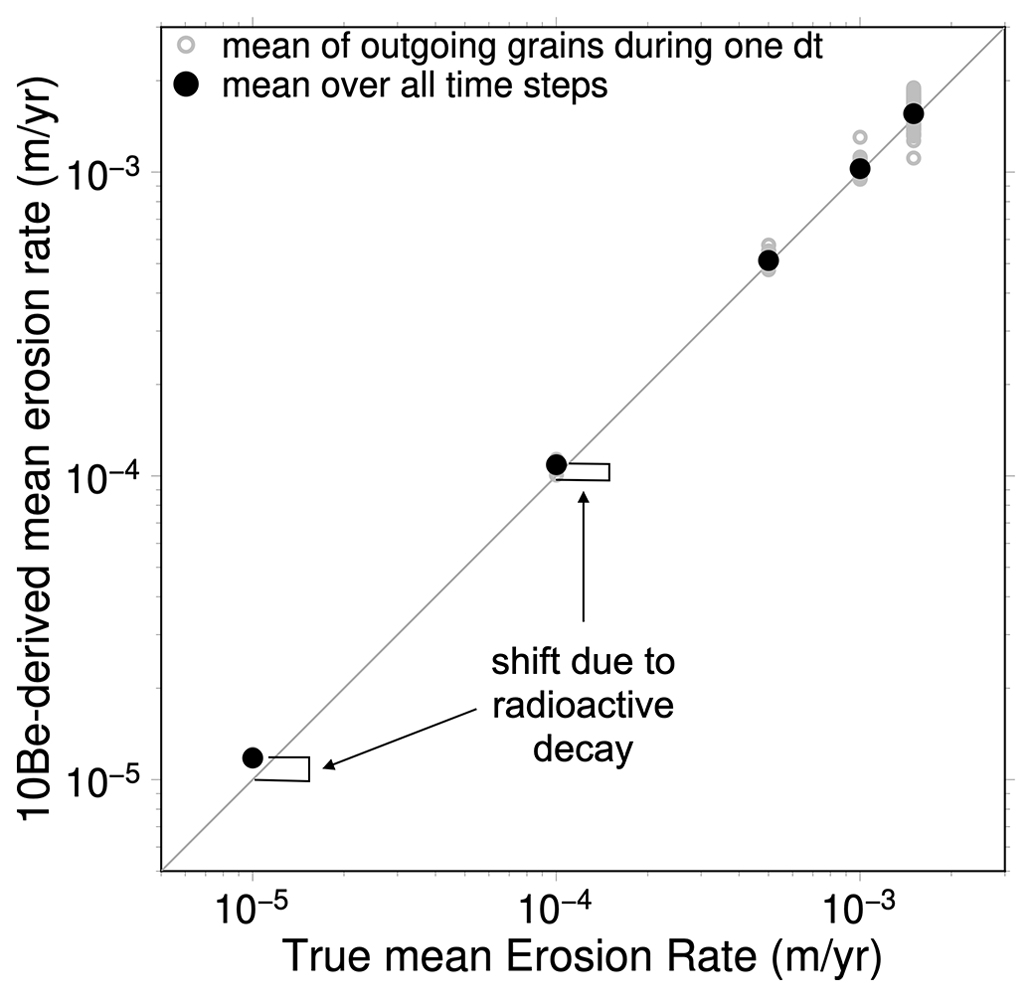
Figure 2 Comparison between the true (calculated from the landscape evolution model in Cidre) black and 10Be-derived erosion rates at dynamic equilibrium () for different values of uplift rates (i.e. different simulations). The overestimation (shift) of the 10Be-derived erosion rates for a low erosion rate (10−5 and 10−4 m yr−1) comes from the absence of radioactive decay in Eq. (14) used to infer the 10Be-derived erosion rates, whereas radioactive decay is taken into account in Cidre. Radioactive decay slightly decreases the mean 10Be concentration. The apparent inferred erosion rate is inversely proportional to the 10Be concentration (Eq. 14), but because it is calculated by neglecting radioactive decay, the apparent inferred erosion rate is slightly overestimated.
4.2 Transient erosion rate
Here, we test the consistency between the true and 10Be-derived erosion rates during the transient stage of the topography adaptation to uplift. We use the same parameters as in the reference simulation described in the previous section. We impose a first 5 Myr period with a constant uplift rate of 1 mm yr−1 and a second 5 Myr-period with a constant uplift rate of 0.1 mm yr−1 which is 10 times lower. The (true) evolution of the mean erosion rate is composed of a transient period and then a dynamic equilibrium where ϵ=U on each cell (Fig. 3a). During the first period, the transient period begins with the establishment of a drainage network and then an increase in the slopes leading to an increase in the mean erosion rate with a classic convex curve, before reaching the dynamic equilibrium (Fig. 3a) (Bonnet and Crave, 2003; Carretier et al., 2009). The maximum dynamic equilibrium elevation reaches 1800 m. In the second period, the mean erosion rate decreases to match the lower uplift rate value at the new dynamic equilibrium. The maximum elevation is 340 m during this new equilibrium period.
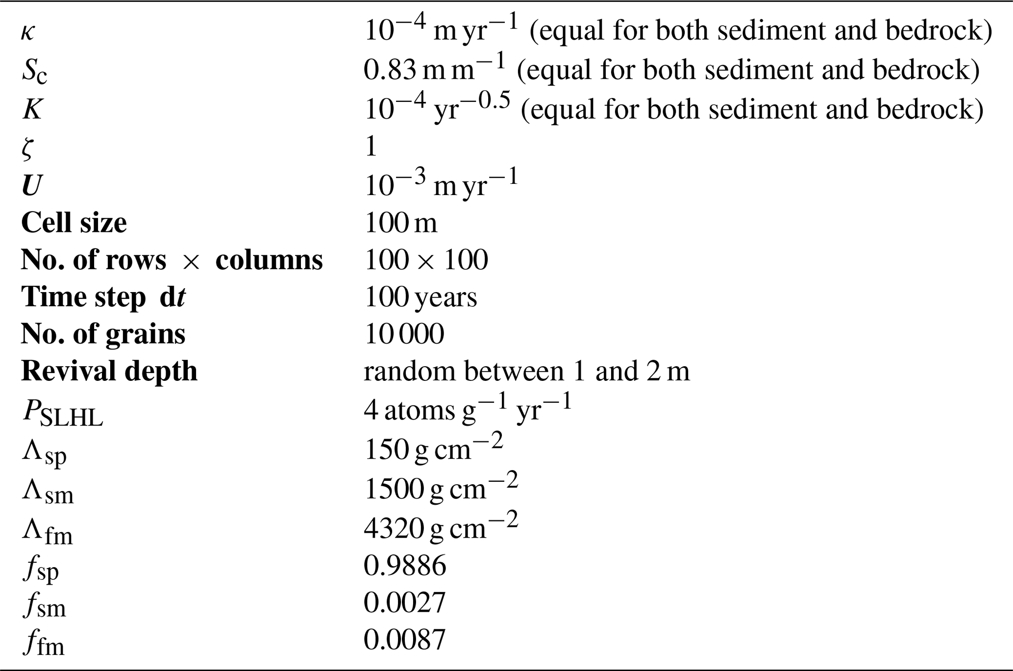
Table 1 Model parameters used in the reference simulation. Parameters written in bold are those that are varied in the other simulations.
At the beginning of the simulation, we spread 10 000 grains of quartz with a radius of 1 mm (1 per cell on average) at a randomly chosen location and depth, where the depth is between 3 and 6 m. Their initial Co=0 at g−1. Contrary to previous simulations, where grains left definitively the model grid, we recycle them each time they leave the model grid. The grains are exhumed and transported, and when they leave the model grid, they are set back to their initial cell at random depths between 1 and 2 m. A grain is set back with a 10Be concentration Co corresponding to the steady-state concentration (Eq. 13) calculated using the current erosion rate of the cell where the grain is set back. The minimum depth of 1 m ensures that most of the 10Be acquisition (79 %) occurs later. This depth will be evaluated later.
Figure 3b shows three snapshots of the topography and grains at 0.35, 5 and 10 Myr. In Fig. 3b, the larger cubes show grains that are in movement during the last time step, whereas the smaller ones show grains still in the bedrock at depth. The first snapshot corresponds to the period of drainage network growth (see Fig. 3a). Not all cells are connected to the imposed outlet, and therefore, the divide of the associated catchment is expanding towards the boundary of the model grid. The 5 Myr step is the topography at dynamic equilibrium with a homogeneous and constant erosion rate of 1 mm yr−1. The 10 Myr snapshot corresponds to the dynamic equilibrium of the second period with a final mean denudation rate of 0.1 mm yr−1, and consequently a lower elevation (see Fig. 3a).
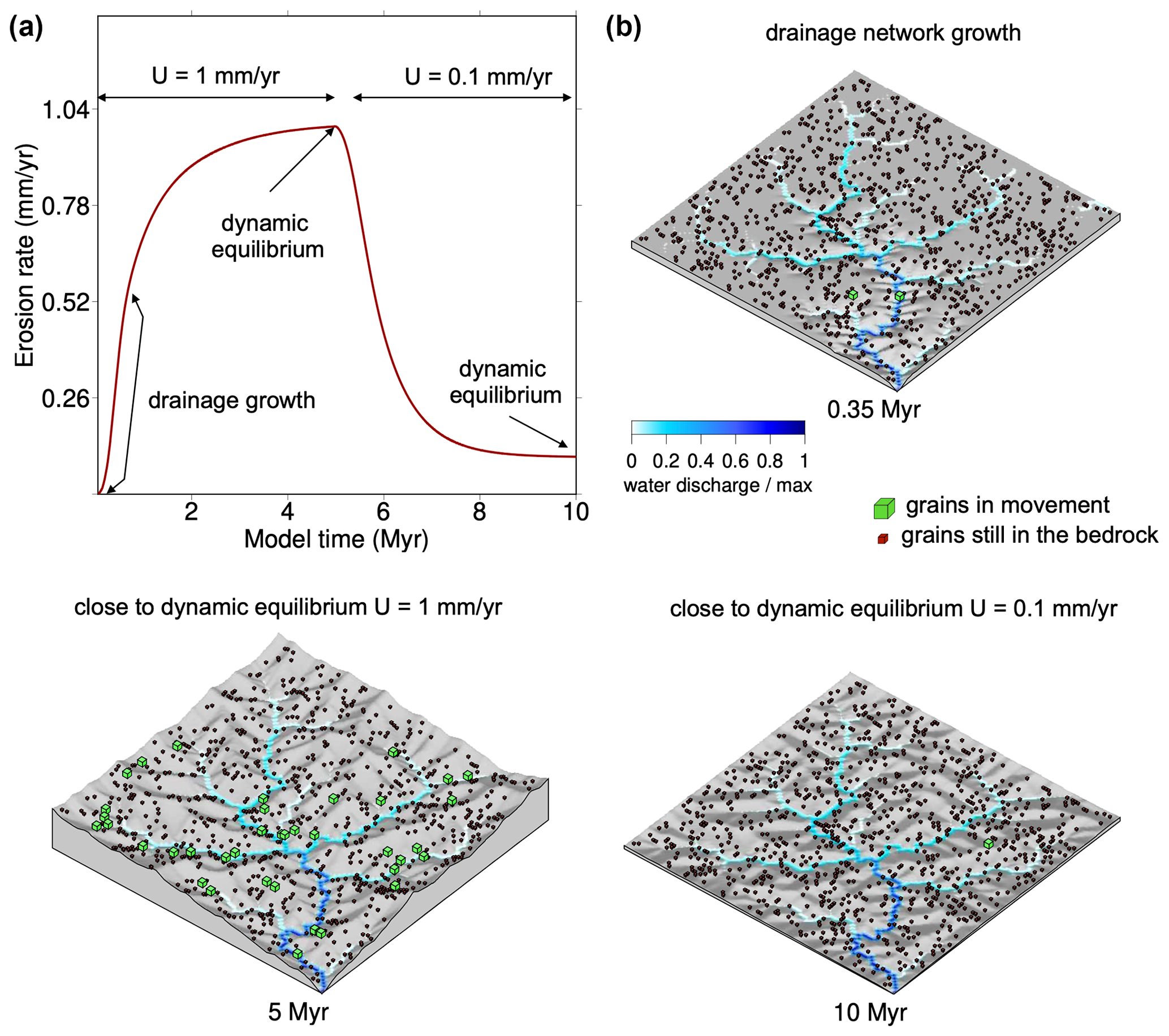
Figure 3 Reference simulation. Panel (a)shows the evolution of the mean erosion rate evolution with two periods of constant uplift rates. Panel (b) is a snapshot of three stages in the topographic evolution. The number of displayed grains is divided by 10 for easier viewing.
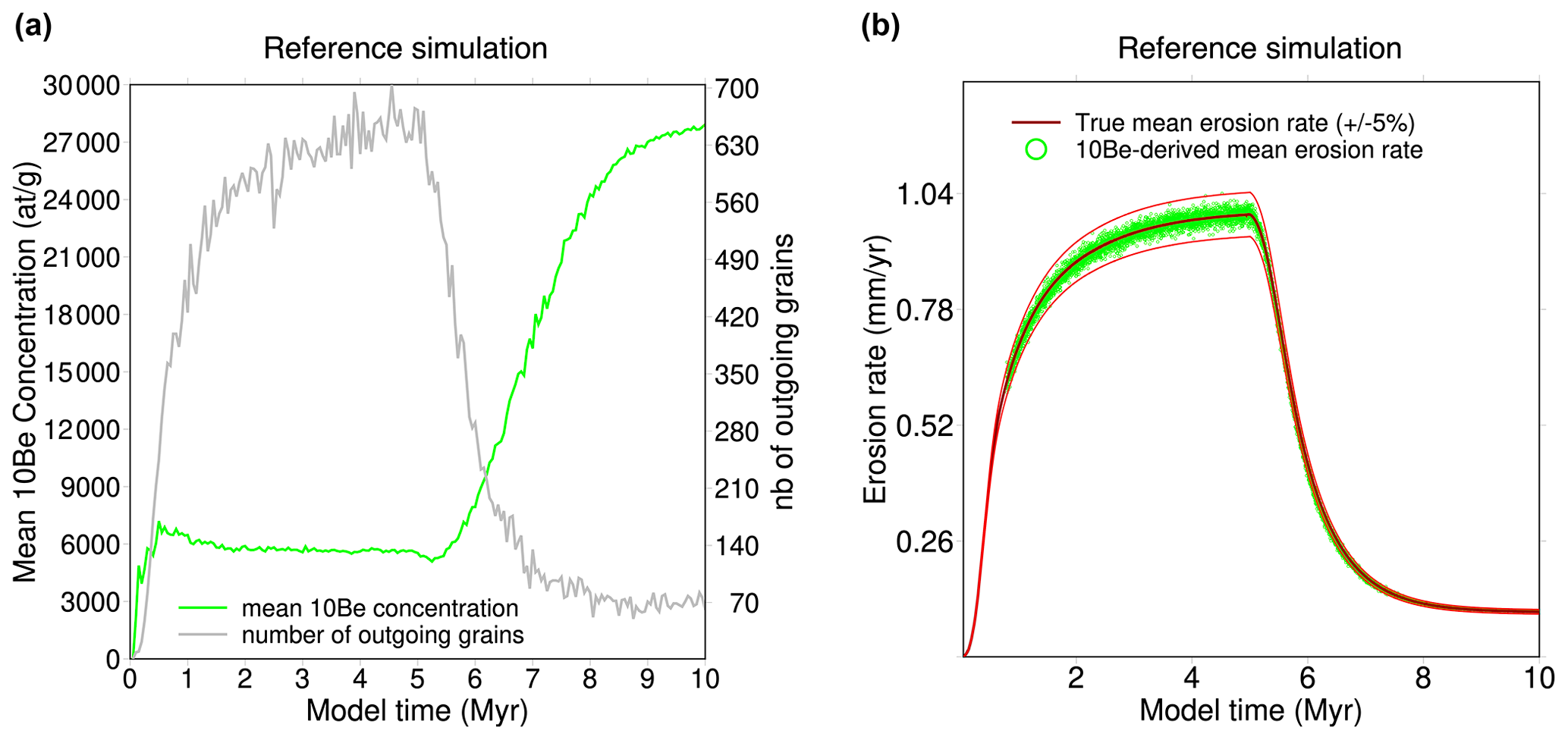
Figure 4 Reference simulation. Panel (a) shows the evolution of the number of outgoing grains during a time step (100 years) and the mean 10Be concentration averaged over the outgoing grains. Panel (b) shows the true mean erosion rate calculated by Cidre and the mean 10Be-derived erosion rate calculated from the mean 10Be concentration of outgoing grains.
The number of grains leaving the model grid at each time step increases through time in the first period (Fig. 4a) because the mean erosion rate increases (Fig. 4b). During the second period, the mean erosion rate decreases and so does the number of grains leaving the model grid (Fig. 4). The mean 10Be concentration increases in the first hundreds of thousands of years because, during the progressive establishment of the drainage network, many grains have stayed in the former surface for a long time before being exported out of the catchment. During the uplift of this surface, the 10Be production rate increases. The long residence time at shallow depth and increasing 10Be production rate have produced grains with high 10Be concentrations, which explains the increase in the mean 10Be concentration during network growth. Once the drainage network is completely established, the 10Be concentration decreases slightly and stabilizes to a nearly constant value, although the erosion rate increases rapidly: the increase in the 10Be production rate due to the increasing elevation is compensated by a decrease in the residence time of the grains as the erosion rate increases. This evolution illustrates that a record showing a constant 10Be concentration may not be a diagnostic for a constant erosion rate. During the second period, the mean concentration in 10Be increases because, although the elevation and thus the 10Be production rate decrease, the 10Be mean concentration is dominated by the longer residence time of grains following the decrease in erosion rate.
Figure 4a shows that the mean 10Be concentration of grains leaving the outlet does not depend on the number of grains, and high frequency variations in this number from one time step to another generate smaller variations in the mean 10Be concentration. The continuous and smooth evolution of the mean 10Be concentration shows that the outgoing grains correctly sample the model grid although they are 14–100 times less numerous than the model cells, even during the transient periods where the erosion rate is heterogeneous.
We now use the mean 10Be concentration of the grains leaving the catchment during a time step to calculate the catchment-averaged erosion rate through time using Eq. (14). is not calculated if the number of grains is smaller than 20. Furthermore, is not calculated during the development of the drainage network for practical reasons as the catchment is smaller than the whole model grid. Each 10Be-derived value corresponds to the average of outgoing grains over a time step of 100 years. Figure 4c shows the good match between the true mean erosion rate and through time. The variation in 10Be-derived is less than 5 % around the true value for the two periods.
Doubling the initial number of grains decreases the scattering to 1 % around the true value, while halving the number of grains increases it to 5 % (Fig. 5).
Decreasing the time step to 20 years increases the scattering to 5 % because there are fewer grains leaving the model grid during a time step (Fig. 6). There is also a very slight (∼ 1 %) overestimation of the mean erosion rate on average when it becomes larger than about 0.8 mm yr−1 because a small time step increases the probability for a grain to be temporarily stored in a cell. Grains coming from cells far from the outlet may take several time steps to reach the outlet once they are detached from the bedrock. A grain close to the outlet may take less time. Consequently, there are proportionately more grains coming from cells close to the outlet. As these grains are located at lower elevations, with smaller 10Be production rates and thus smaller 10Be concentrations, the mean 10Be concentration of the outgoing grains is slightly underestimated. In turn, the 10Be-derived erosion rate is slightly overestimated.
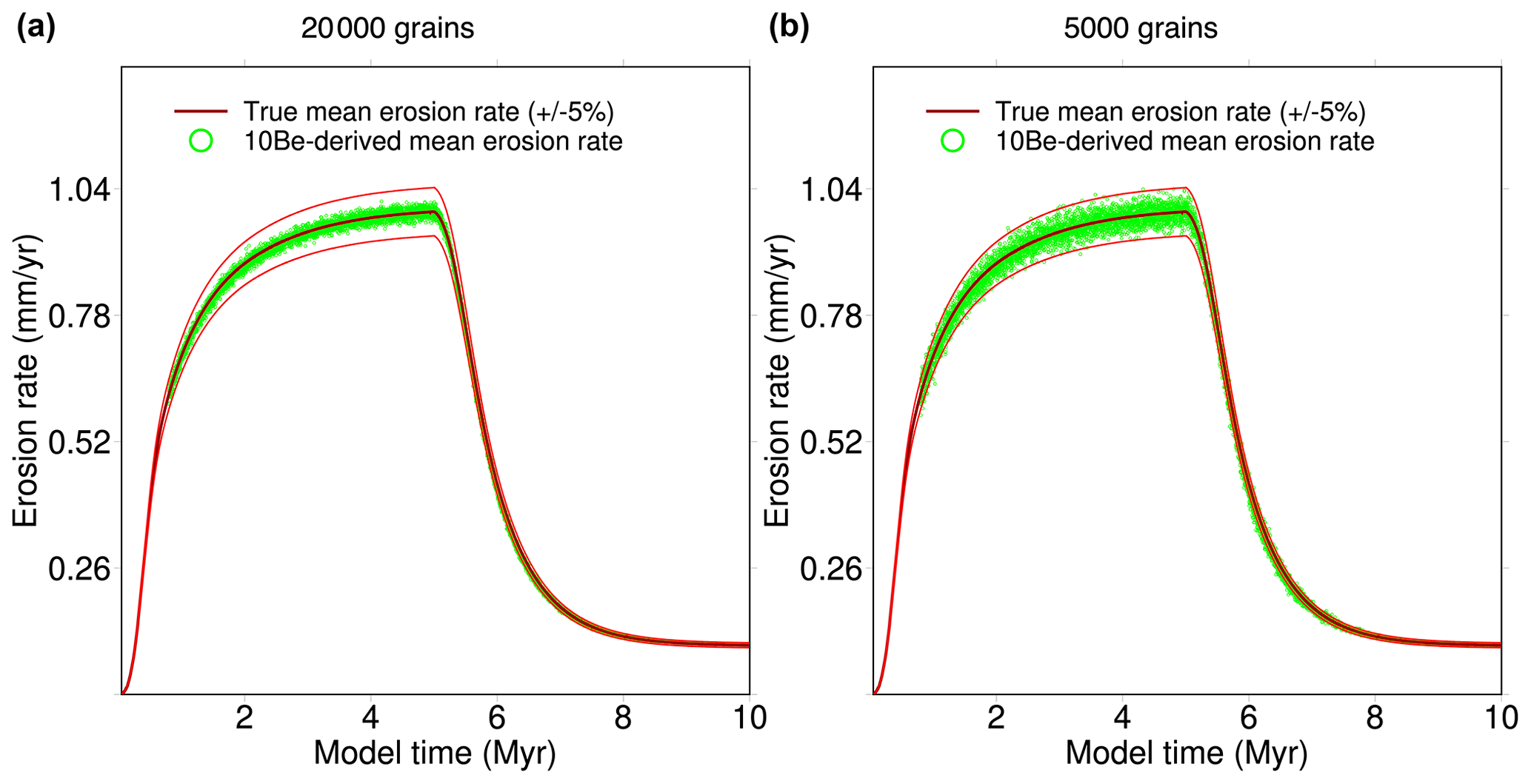
Figure 5 Effect of seeding the model with a different number of grains on the mean 10Be-derived erosion rate calculated from the mean 10Be concentration of outgoing grains. Panel (a) represents 20 000 grains (two per cell on average). Panel (b)represents 5000 grains (one out of every two cells on average).
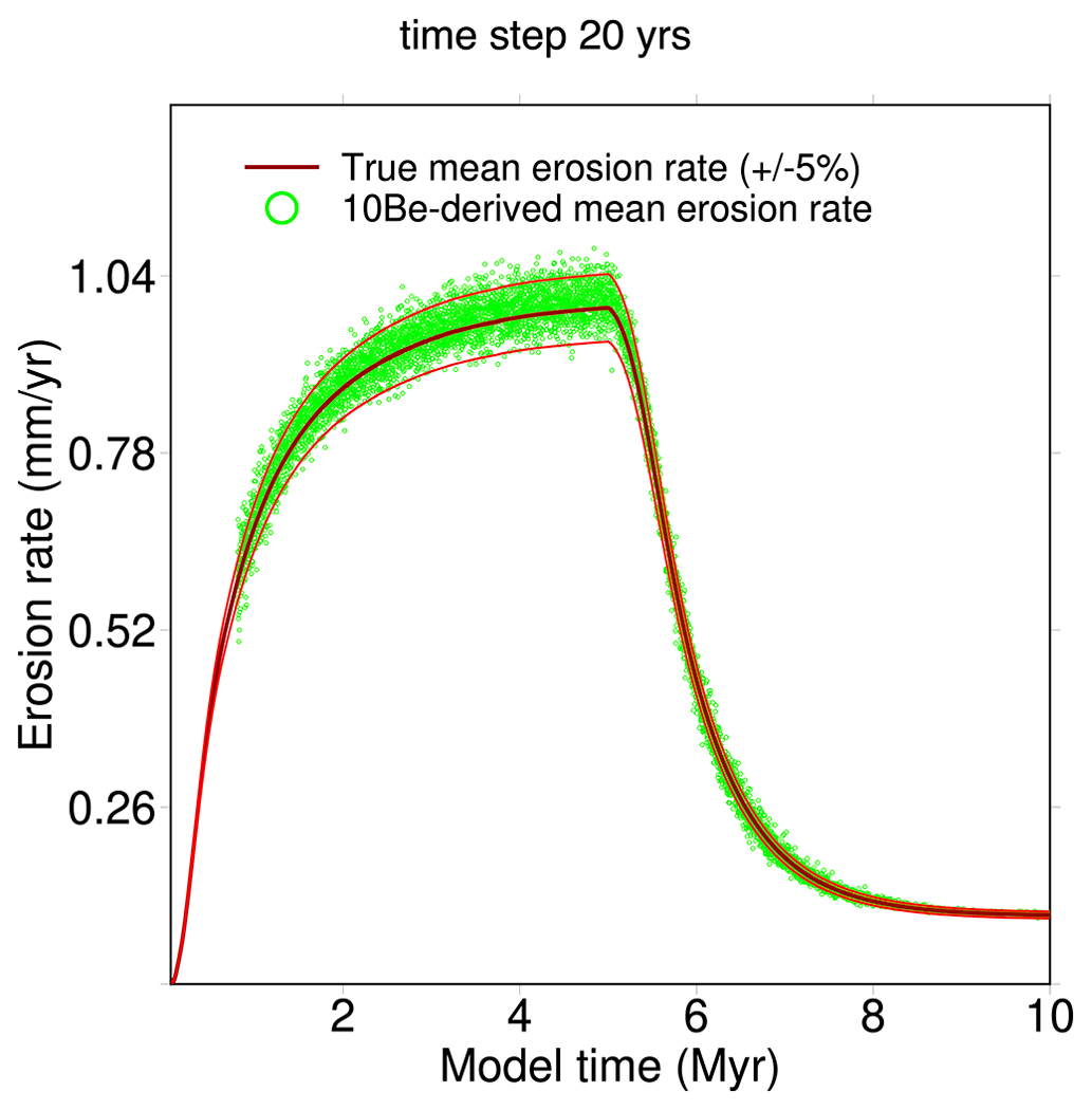
Figure 6 Effect of dividing the calculation time step by 10 on the mean 10Be-derived erosion rate calculated from the mean 10Be concentration of outgoing grains. The variability in the mean 10Be-derived erosion rate increases because there is a smaller number of outgoing grains over a smaller time step.
As LEMs can be sensitive to cell size, we tested the result of decreasing the cell size to 25 m, and the time step to 50 years does not change the goodness of fit between the 10Be-derived and true (Fig. 7).
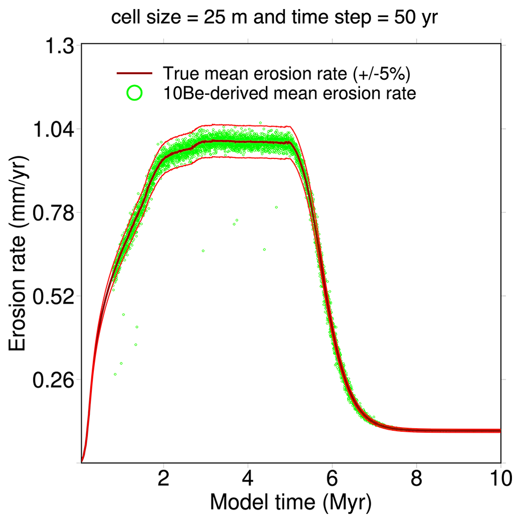
Figure 7 Effect of decreasing the cell size to 25 m (keeping the same number of cells) on the mean 10Be-derived erosion rate calculated from the mean 10Be concentration of outgoing grains. The different shape of the denudation curve compared with the reference simulation in Fig. 4 comes from the increase in slopes in this simulation due to the smaller cell size, leading to a larger contribution of hillslope processes when the slope approaches the critical slope Sc in Eq. (4).
In order to test the effect of catchment size on the calculation of 10Be-derived , we use a model grid with 200×200 cells, which is four times larger than the reference simulation, but we leave the other parameters as in the reference simulation. We seed the model grid with 40 000 grains, i.e. one per cell on average, as in the reference simulation. Figure 8 shows the good match between the 10Be-derived and the true value in this case too. The smaller variability in the 10Be-derived around the true value is due to the fact that there are four times more grains that leave the grid at each time step.
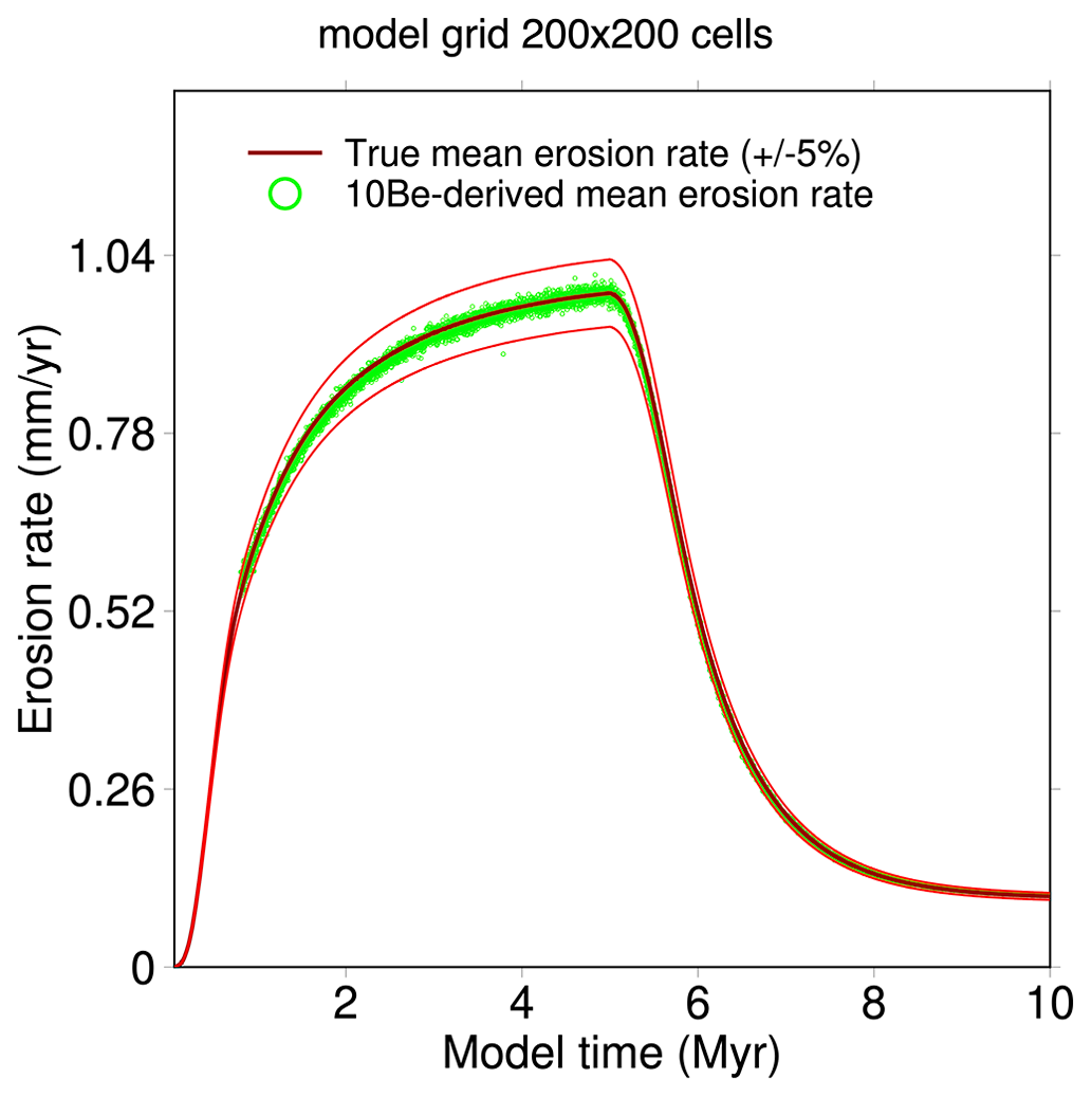
Figure 8 Effect of multiplying the model grid size by four on the mean 10Be-derived erosion rate calculated from the mean 10Be concentration of outgoing grains. The number of grains is also multiplied by four to have one grain per cell on average as in the reference simulation.
We now rerun the reference simulation but divide the uplift rate by 10 in the two periods. Figure 9a shows that the 10Be-derived is overestimated by approximately 2 % during the dynamic equilibrium of the first period (4–5 Myr). This is due to the model in Eq. (14) used to calculate that neglects the radioactive decay. Here, radioactive decay influences the 10Be concentration because the clast residence time in the bedrock is longer for small uplift rates (Lal, 1991). In the second period, the 10Be-derived erosion rate is overestimated by roughly 20 % during the transient adjustment to a smaller uplift rate (6–8 Myr). This overestimation comes from the delayed response of CN for a low erosion rate. The response time to adjust to a new erosion rate ϵ is about four times when only considering CN produced by spallation (Lal, 1991). With ϵ between 0.1 and 0.01 mm yr−1, the response time is between 60 000 and 600 000 years. Consequently, the CN concentration is out of phase during the rapid transient decrease in the erosion rate for the second period. This delay was not observed in the reference simulation because the response times were 10 times shorter. Furthermore, the variability in 10Be-derived tends to increase for smaller uplift rates because the number of outgoing grains is smaller at each time step. In this simulation, the number of outgoing grains varies between 100 and 10. It is remarkable that with such a small number of grains (particularly during the second period with a very low uplift rate), the 10Be-derived remains a good estimate of the true . When the number of grains is multiplied by four, this decreases the variability (Fig. 9b).
As there is a rapid decrease in the erosion rate, but a long residence time of grains in the last metres because the erosion rates are low in these last simulations, one may question the chosen revival depths of the grains because they may be too shallow to record the previous decrease in erosion. We test this by changing the revival depth of the grains to between 2 and 4 m. Figure 9c shows that the delay in the 10Be-derived erosion rate between 6 and 8 Myr is similar, with a larger variability due to the smaller number of outgoing grains at each model time.
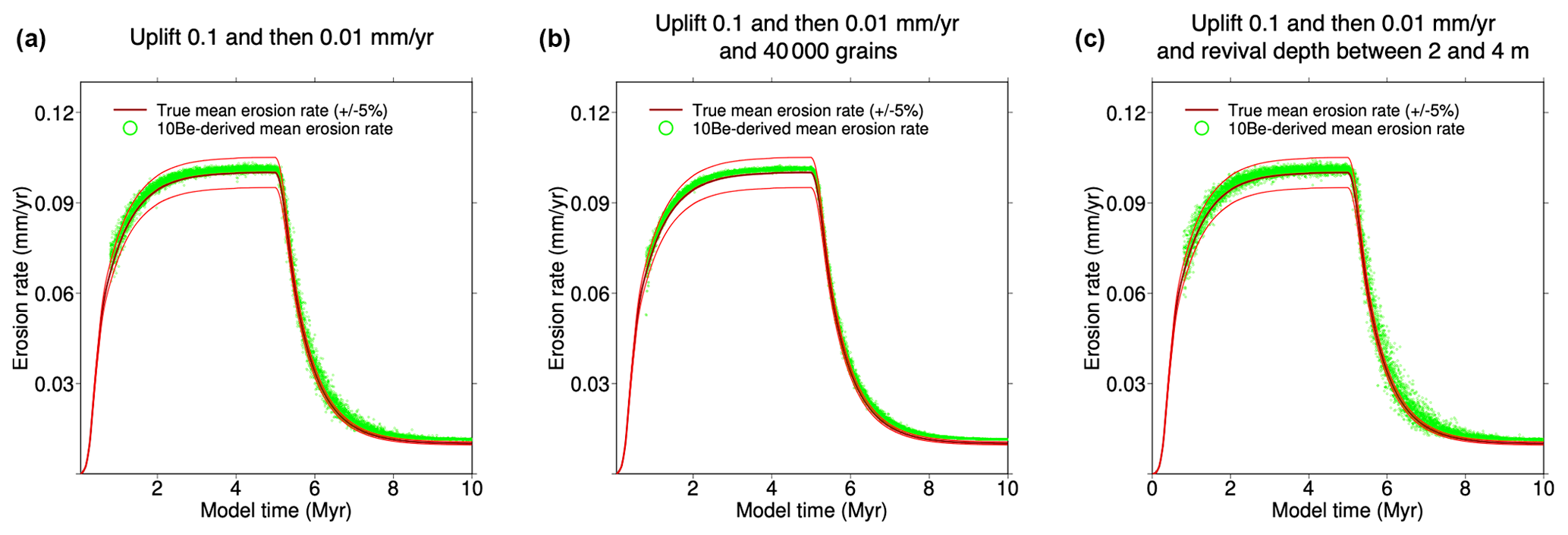
Figure 9 Effect of an uplift rate that is 10 times smaller. In (a) the number of grains is 10 000 as in the reference simulation. In (b) the number of grains is 40 000. In (c) the number of grains is 10 000, but the (revival) depth at which the grains are set back to the model grid is between 2 and 4 m instead of 1 and 2 m. In the three cases, the slight 1 %–2 % overestimation of the 10Be-derived erosion rate during the first dynamic equilibrium stage (4–5 Myr) comes from the model used to derive erosion rates that neglect the 10Be radioactive decay, which only matters for low erosion rates. During the second period (6–8 Myr), there is a significant overestimation of the true erosion by approximately 20 %. This overestimation comes mainly from the delayed response of the CN concentration for a low erosion rate. In (c) the variability is larger because there are fewer grains going out at each model time step.
In order to further test if a revival depth between 1 and 2 m gives good results, we carried out three final simulations using the parameters of the reference simulation but imposing a constant uplift rate of 0.1 mm yr−1 and an oscillatory precipitation rate between 0.5 and 1 m yr−1 during 10 Myr. The three simulations correspond to three different periods of oscillation constituting the Milankovitch cycles: 23, 41 and 100 kyr. It is predicted that the 10Be-derived erosion rate should be shifted with a lag that increases with the period of oscillation (Schaller and Ehlers, 2006). Figure 10 illustrates several cycles in the last 200 kyr of these simulations. It shows that the lag between the 10Be-derived and true erosion rate signals increases with the oscillation period. The lags are very similar to the ones found by Schaller and Ehlers (2006) in the case of one-point source simulations for the same oscillation periods, magnitude and true erosion rates (see Fig. 5d, e and f in Schaller and Ehlers, 2006). We also observe that the amplitude of the 10Be-derived erosion rate decreases when the frequency of the true erosion rate variation increases, consistent with the results of Schaller and Ehlers (2006). Indeed, when a grain reaches shallow depths (< 1 m) during a low erosion rate period, its 10Be concentration is relatively high. If the grain is then rapidly exhumed, it will reach the surface with a concentration that is too high compared with what it would have been with a high rate of erosion. Once detached, if we use this concentration to determine an erosion rate, we underestimate the erosion rate. This memory effect causes the cosmogenic signal to be damped out.
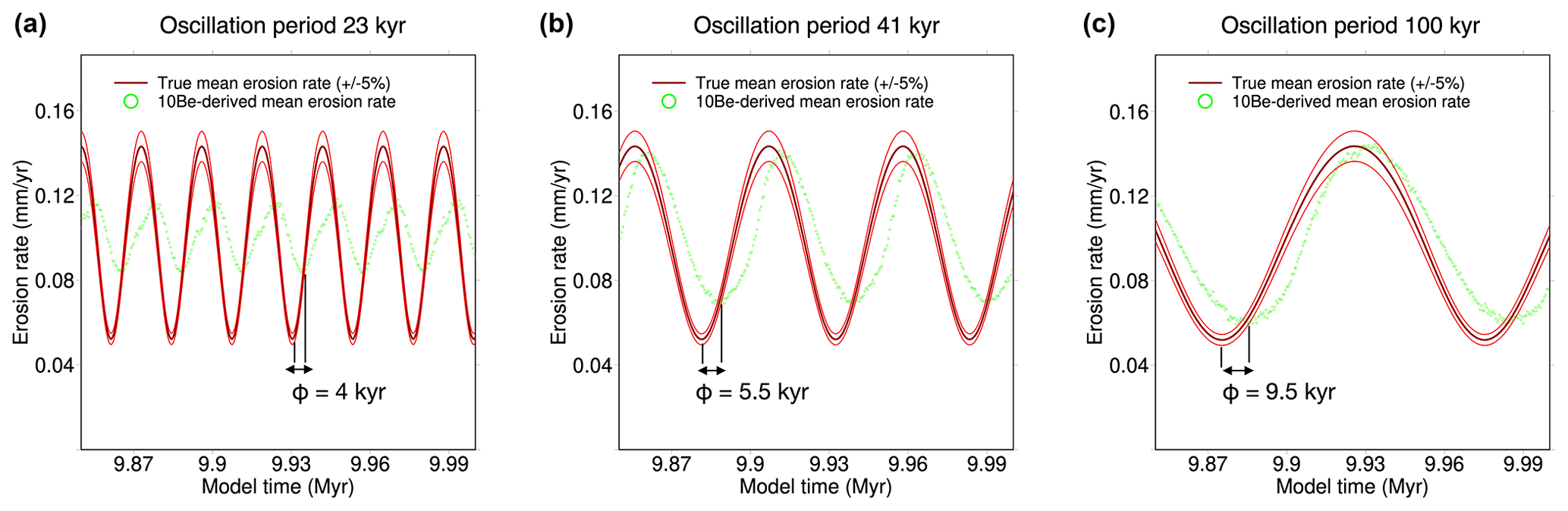
Figure 10 Simulations using the parameters of the reference simulation but a constant uplift rate of 0.1 mm yr−1 and oscillations of the precipitation rates between 0.5 and 1 m yr−1 with different periods: (a) 23 kyr, (b) 41 kyr and (c) 100 kyr. The observed lags ϕ are similar to the ones calculated by Schaller and Ehlers (2006) for similar conditions but for a theoretical one-point source catchment. This consistency shows that the revival procedures of grains at depths between 1 and 2 m give robust results.
5.1 Limitations and advantages
The main limitation of this approach deals with the computational time when the number of grains is large. Some study cases may require a huge number of grains. In practice, the feasibility of these simulations will depend on the computation facilities. To give an indication, the reference simulation with 100×100 cells and 10 000 grains runs in half an hour on a personal computer. The simulation with a grid and number of grains four times larger runs in 2.5 h. Parallelism of the grains' calculation is straightforward as they are independent of each other and would decrease the running time. As the precision of the results depends on the number of grains, the model can be adapted according to the studied process. For example, a higher density of grains is required to study the CN detrital signal associated with climate variations for the 20 kyr period compared with the density required for variations in the 100 kyr period. It is possible to determine a simple quality control of the results by setting a minimum number of grains leaving the model grid to interpret the CN concentrations. Beyond the number of grains, the choice of time step and revival depths have an influence on the resulting cosmogenic concentrations, but the simulations presented here show that these choices do not imply variations in inferred erosion rates larger than 10 % around the true value (when the CN and the erosion rate signals are in phase). This error remains smaller than or equal to the uncertainty of the CN-derived erosion rate in most cases, given the external uncertainties on the CN production rates (Balco et al., 2008).
In the current implementation, grains do not physically erode during their transport (but they can weather and decrease in size chemically; Carretier et al., 2018). In the real world, attrition can significantly change the CN concentration within and at the surface of decimetric pebbles. In the model, this would require tracking the CN concentration of the layers within the pebbles. This was done in the model of Carretier and Regard (2011), which served as a basis for the grain model in Cidre; therefore, it would be straightforward to implement it in Cidre as well.
Modelling deep landslides (Campforts et al., 2020) would be a limitation to the grain revival process. If the specified maximum depth at which a grain is set back to the grid is much smaller than the thickness of the landslides, there is a risk that the mean CN concentration of grains in the landslide would overestimate the mean value of the landslide. In such cases, the maximum revival depth of the grains must be adequately adapted to be greater than the maximum landslide thickness.
The revival of dead grains is a useful approach for the statistics of CN at the catchment outlet, but this approach is an approximation. It is fundamental that the depth at which the grains are set back to the model grid be much larger than the attenuation length of production by spallation ( 65 cm in granitic rocks). If not, there is a risk that the revival CN concentration Co of the grain would be a very poor approximation of the erosion history of its cell if the erosion rate has decreased very quickly and with a huge magnitude. Figure 10 shows that setting back the outgoing clasts at depths larger than 1 m with the 10Be concentration corresponding to the equilibrium value with the local erosion rate gives robust results.
In a Lagrangian formulation of CN concentration evolution, the approach by discrete grains has advantages. The alternative Eulerian approach would require calculating and tracking the concentration of CNs at different depths below each cell at each time step (Niemi et al., 2005). Petit et al. (2023) present a simplified approach implemented in the LEM Badlands model based on the computation of the CN concentration at the earth's surface only without calculating the CN concentration profile at depth. This level of simplification is required in this case for practical reasons of computation in an LEM. Tracking the whole depth profile evolution in the whole model grid cell where erosion and deposition can alternate at each iteration would be prohibitive in terms of computational time and would be difficult to implement (Petit et al., 2023). One advantage of the Lagrangian approach is that it can tackle more complex erosion–deposition scenarios compared with the Eulerian approach (Knudsen et al., 2019). For example, it is simpler to calculate the evolution of a given grain experiencing a complex erosion–deposition history of the surface above it rather than the evolution of a (deep) depth profile of the concentration for each time step below a surface that is constantly changing in terms of elevation. From the grain's point of view, it is easy to calculate the evolution of CN in the grain when it is stored, buried and eroded again stochastically, or when the soil above it is alternatively eroded or buried, as only the grain's depth has to be adapted. (Note that the difference in density between rock and sediment is not taken into account when calculating the CN production rate in the simulations presented in this work, but it is possible to simply implement this.) The Eulerian approach requires tracking the sources, and averaging the concentration from these different sources in cells during the transport of sediment, assuming perfect mixing. This process loses some information about the distribution of CN for a population of grains. On the contrary, the distribution of the CN concentration is fully conserved by treating the grains separately. One drawback to the grain-by-grain approach is that the average CN concentration of the transported sediment is not precisely known, with an uncertainty that decreases with the number of grains. On the other hand, when the full distribution of the CN concentrations of a population of grains is known, then it becomes possible to study part of the stochasticity of erosion–deposition processes on hillslopes and in rivers, including the long-term temporary storage of some grains that may contribute significantly to the CN concentration average (Carretier et al., 2019). The potential applications of this are described below.
5.2 Potential applications
The method using CN in riverine sediment to quantify modern and palaeo catchment-averaged denudation rates assumes that the CN concentrations of any grain have been entirely acquired on the hillslopes. Yet, the temporary storage and recycling of sediment grains between the eroding sources and sedimentary basins may change their CN concentration depending on the considered nuclide or the climatic context (Wittmann and VonBlanckenburg, 2009; Carretier et al., 2019). Storage and recycling can delay or obscure the transmission of an erosion signal from source to sink (Carretier et al., 2020; Tofelde et al., 2021). Detrital signals in the CN concentrations can also be used positively to study the erosion–deposition processes on hillslopes (Slosson et al., 2022), burial histories in basins (Balco et al., 2013; Sanchez et al., 2021), the distribution of residence times and transport lengths in rivers (Carretier et al., 2019) or to infer the palaeo-denudation rates of mountains (Charreau et al., 2011). Nevertheless, linking a CN detrital signal with landscape evolution is not straightforward. A forward model, such as Cidre, which simulates CN in distinct grains that move stochastically, would help. For example, the conclusions of several studies on palaeo-denudation rates over the Pliocene–Pleistocene periods suggest either constant or modest variations in the denudation rate in Asia or in the Andes (Charreau et al., 2011; Madella et al., 2018; Lenard et al., 2020; Charreau et al., 2021), or a significant change recorded in the last glacial cycle in river terraces or at the outlet of small mountainous catchments (Schaller et al., 2002; Mariotti et al., 2021). Some factors that should be explored numerically with a numerical model, such as Cidre, to better understand the CN detrital signals (Petit et al., 2023) include the following: the effect of catchment size, uplift rate or grain size; whether a flood plain is present or not; the frequency of climatic variations; and variations in the elevation of the eroded sources.
Cidre includes the possibility to produce a regolith corresponding to the weathering of the underlying bedrock (Carretier et al., 2014, 2018). Once a grain is located in the regolith during its exhumation on the hillslopes, it continues to be exhumed towards the surface until it is detached. Alternatively, its depth could be chosen randomly at each time step to simulate bioturbation or physical creep within the soil. This option is easy to implement and would make it possible to analyse the effect of different soil processes on the riverine detrital CN signal within the framework of reservoir theories (Mudd and Yoo, 2010).
One of the advantages of modelling grains is the simplicity in tracking the evolution of distinctive cosmogenic nuclides, taking advantage of their different radioactive decay rates. When grains experience complex temporary burial and recycling histories, their initial concentration ratio on hillslopes varies downstream. It would be also quite simple to implement the evolution of the meteoritic 10Be concentration at the surface of the grains, or their optically stimulated luminescence (OSL) dosimetry based on Guyez et al. (2023). The distributions of various CN concentrations in a river sample, e.g. 10Be, 26Al and 14C, contain information about possible past changes in the catchment-averaged erosion rates and residence times in fluvial systems (Repasch et al., 2020; Ben-Israel et al., 2022). We need to establish a link between erosion rate changes and the detrital CN concentrations in different nuclides and potentially other properties such as OSL dosimetry. Doing so may allow us to address recent changes over the past few centuries associated with natural and anthropic modifications of the landscape.
We present a new coupling of the landscape evolution model Cidre with a model of CN concentrations in individual grains. The algorithm is tested by comparing the catchment-averaged erosion rate derived from the 10Be concentration of grains leaving an uplifting catchment and the true catchment-averaged erosion rate calculated by Cidre. The main limitation is the number of grains that has to be set in a simulation to achieve the desired precision. The catchment-average erosion rates are approximated to within 5 % uncertainty in most of the cases with a limited number of grains. This Lagrangian approach allows us to fill the gap that exists between landscape modelling, which is used to help understand variations in the elevation and erosion of landscapes, and field data, which often correspond to the CN concentrations of grains in a soil or river sample.
The Cidre source codes are available here https://gitlab.com/geomorphotoulouse/cidre (last access: September 2023) under the opensource CeCILL v2.1 licence. The code is also permanently deposited on the HAL repository with the number hal-04141239v1 (https://hal.science/hal-04141239, Carretier et al., 2023). No data sets were used in this article.
SC and VR designed the study and the cosmogenic nuclide model. SC and YA implemented the cosmogenic nuclide model with the help of BP. SC wrote the paper with input from all the co-authors.
The contact author has declared that none of the authors has any competing interests.
Publisher's note: Copernicus Publications remains neutral with regard to jurisdictional claims made in the text, published maps, institutional affiliations, or any other geographical representation in this paper. While Copernicus Publications makes every effort to include appropriate place names, the final responsibility lies with the authors.
We thank Marc De Rafelis for useful discussions. This research was supported, in part, by the French ANR, and the WIVA, PANTERA and WEARING-DOWN projects. We thank Carole Petit and Rebekah Harries for their useful reviews.
This research has been supported by the Agence Nationale de la Recherche (WIVA, WEARING DOWN and PANTERA grants).
This paper was edited by Andrew Wickert and reviewed by Carole Petit and Rebekah Harries.
Balco, G., Stone, J., Lifton, N., and Dunai, T.: A complete and easily accessible means of calculating surface exposure ages or erosion rates from 10Be and 26Al measurements, Quat. Geochronol., 3, 174–195, 2008. a, b
Balco, G., Soreghan, G. S., Sweet, D. E., Marra, K. R., and Bierman, P. R.: Cosmogenic-nuclide burial ages for Pleistocene sedimentary fill in Unaweep Canyon, Colorado, USA, Quat. Geochronol., 18, 149–157, https://doi.org/10.1016/j.quageo.2013.02.002, 2013. a
Ben-Israel, M., Armon, M., Matmon, A., and ASTER Team: Sediment Residence Times in Large Rivers Quantified Using a Cosmogenic Nuclides Based Transport Model and Implications for Buffering of Continental Erosion Signals, J. Geophys. Res.-Earth, 127, e2021JF006417, https://doi.org/10.1029/2021JF006417, 2022. a, b
Bonnet, S. and Crave, A.: Landscape response to climate change: Insights from experimental modeling and implications for tectonic versus climatic uplift of topography, Geology, 31, 123–126, https://doi.org/10.1130/0091-7613(2003)031<0123:LRTCCI>2.0.CO;2, 2003. a
Braucher, R., Colin, F., Brown, E., Bourles, D., Bamba, O., Raisbeck, G., Yiou, F., and Koud, J.: African laterite dynamics using in situ-produced Be-10, Geochim. Cosmochim. Ac., 62, 1501–1507, https://doi.org/10.1016/S0016-7037(98)00085-4, 1998. a
Braucher, R., Brown, E., Bourlès, D., and Colin, F.: In situ produced 10Be measurements at great depths: implications for production rates by fast muons, Earth Planet. Sc. Lett., 211, 251–258, https://doi.org/10.1016/S0012-821X(03)00205-X, 2003. a
Braucher, R., Merchel, S., Borgomano, J., and Bourlés, D.: Production of cosmogenic radionuclides at great depth: A multi element approach, Earth Planet. Sc. Lett., 309, 1–9, https://doi.org/10.1016/j.epsl.2011.06.036, 2011. a, b
Brown, E. T., Stallard, R. F., Larsen, M. C., Raisebeck, G. M., and Yiou, F.: Denudation rates determined from the accumulation of in situ-produced 10Be in the Luquillo Experimental Forest, Puerto Rico, Earth Planet. Sc. Lett., 129, 193–202, 1995. a, b
Campforts, B., Shobe, C. M., Steer, P., Vanmaercke, M., Lague, D., and Braun, J.: HyLands 1.0: a hybrid landscape evolution model to simulate the impact of landslides and landslide-derived sediment on landscape evolution, Geosci. Model Dev., 13, 3863–3886, https://doi.org/10.5194/gmd-13-3863-2020, 2020. a
Carretier, S. and Regard, V.: Is it possible to quantify pebble abrasion and velocity in rivers using terrestrial cosmogenic nuclides?, J. Geophys. Res.-Earth, 116, F04003, https://doi.org/10.1029/2011JF001968, 2011. a
Carretier, S., Regard, V., and Soual, C.: Theoretical cosmogenic nuclide concentration in river bedload clasts : Does it depend on clast size?, Quat. Geochronol., 4, 108–123, https://doi.org/10.1016/j.quageo.2008.11.004, 2009. a, b, c
Carretier, S., Goddéris, Y., Delannoy, T., and Rouby, D.: Mean bedrock-to-saprolite conversion and erosion rates during mountain growth and decline, Geomorphology, 209, 29–52, https://doi.org/10.1016/j.geomorph.2013.11.025, 2014. a
Carretier, S., Martinod, P., Reich, M., and Godderis, Y.: Modelling sediment clasts transport during landscape evolution, Earth Surf. Dynam., 4, 237–251, https://doi.org/10.5194/esurf-4-237-2016, 2016. a, b, c, d, e, f
Carretier, S., Goddéris, Y., Martinez, J., Reich, M., and Martinod, P.: Colluvial deposits as a possible weathering reservoir in uplifting mountains, Earth Surf. Dynam., 6, 217–237, https://doi.org/10.5194/esurf-6-217-2018, 2018. a, b, c
Carretier, S., Regard, V., Leanni, L., and Farias, M.: Long-term dispersion of river gravel in a canyon in the Atacama Desert, Central Andes, deduced from their 10Be concentrations, Sci. Rep., 9, 17763, https://doi.org/10.1038/s41598-019-53806-x, 2019. a, b, c, d, e
Carretier, S., Guerit, L., Harries, R., Regard, V., Maffre, P., and Bonnet, S.: The distribution of sediment residence times at the foot of mountains and its implications for proxies recorded in sedimentary basins, Earth Planet. Sc. Lett., 546, 116448, https://doi.org/10.1016/j.epsl.2020.116448, 2020. a, b
Carretier, S., Plazolles, B., Abdelhafiz, Y., Martinod, P., and Poisson, P.: CIDRE, HAL Archive [code], https://hal.science/hal-04141239, last access: September 2023. a
Charreau, J., Blard, P., Puchol, N., Avouac, J.-P., Lallier-Vergès, E., Bourlès, D., Braucher, R., Gallaud, A., Finkel, R., Jolivet, M., Chen, Y., and Roy, P.: Paleo-erosion rates in Central Asia since 9 Ma: A transient increase at the onset of Quaternary glaciations?, Earth Planet. Sc. Lett., 304, 85–92, https://doi.org/10.1016/j.epsl.2011.01.018, 2011. a, b
Charreau, J., Lave, J., France-Lanord, C., Puchol, N., Blard, P.-H., Pik, R., Gajurel, A. P., and Team, A.: A 6 Ma record of palaeodenudation in the central Himalayas from in situ cosmogenic Be-10 in the Surai section, Basin Res., 33, 1218–1239, https://doi.org/10.1111/bre.12511, 2021. a
Codilean, A., Bishop, P., Stuart, F., Hoey, T., Fabel, D., and Freeman, S.: Single-grain cosmogenic 21Ne concentrations in fluvial sediment reveal spatially variable erosion rates, Geology, 36, 159–162, 2008. a, b
Davy, P. and Lague, D.: The erosion/transport equation of landscape evolution models revisited, J. Geophys. Res., 114, F03007, https://doi.org/10.1029/2008JF001146, 2009. a
DiBiase, R. A.: Short communication: Increasing vertical attenuation length of cosmogenic nuclide production on steep slopes negates topographic shielding corrections for catchment erosion rates, Earth Surf. Dynam., 6, 923–931, https://doi.org/10.5194/esurf-6-923-2018, 2018. a
Dunai, T.: Scaling factors for production rates of in situ produced cosmogenic nuclides: a critical reevaluation, Earth Planet. Sc. Lett., 176, 157–169, https://doi.org/10.1016/S0012-821X(99)00310-6, 2000. a
Dunai, T., Lopez, G., and Juez-Larre, J.: Oligocene-Miocene age of aridity in the Atacama Desert revealed by exposure dating of erosion-sensitive landforms, Geology, 33, 321–324, 2005. a
Dunai, T. J., Binnie, S. A., and Gerdes, A.: In situ-produced cosmogenic krypton in zircon and its potential for Earth surface applications, Geochronology, 4, 65–85, https://doi.org/10.5194/gchron-4-65-2022, 2022. a
Gayer, E., Mukhopadhyay, S., and Meade, B.: Spatial variability of erosion rates inferred from the frequency distribution of cosmogenic He-3 in olivines from Hawaiian river sediments, Earth Planet. Sc. Lett., 266, 303–315, 2008. a
Gosse, J. and Phillips, F.: Terrestrial in situ cosmogenic nuclides: theory and application, Quaternary Sci. Rev., 20, 1475–1560, 2001. a
Guyez, A., Bonnet, S., Reimann, T., Carretier, S., and Wallinga, J.: A Novel Approach to Quantify Sediment Transfer and Storage in Rivers-Testing Feldspar Single-Grain pIRIR Analysis and Numerical Simulations, J. Geophys. Res.-Earth, 128, e2022JF006727, https://doi.org/10.1029/2022JF006727, 2023. a
Knudsen, M. F., Egholm, D. L., and Jansen, J. D.: Time-integrating cosmogenic nuclide inventories under the influence of variable erosion, exposure, and sediment mixing, Quat. Geochronol., 51, 110–119, https://doi.org/10.1016/j.quageo.2019.02.005, 2019. a
Kooi, H. and Beaumont, C.: Large-scale Geomorphology: Classical concepts reconciled and integrated with contemporary ideas via surface processes model, J. Geophys. Res., 101, 3361–3386, 1996. a
Lal, D.: Cosmic ray labeling of erosion surfaces: in situ nuclide production rates and erosion models, Earth Planet. Sc. Lett., 104, 424–439, 1991. a, b, c
Lenard, S. J. P., Lave, J., France-Lanord, C., Aumaitre, G., Bourles, D. L., and Keddadouche, K.: Steady erosion rates in the Himalayas through late Cenozoic climatic changes, Nat. Geosci., 13, 448, https://doi.org/10.1038/s41561-020-0585-2, 2020. a
Lifton, N., Sato, T., and Dunai, T. J.: Scaling in situ cosmogenic nuclide production rates using analytical approximations to atmospheric cosmic-ray fluxes, Earth Planet. Sc. Lett., 386, 149–160, https://doi.org/10.1016/j.epsl.2013.10.052, 2014. a
Madella, A., Delunel, R., Akçar, N., Schlunegger, F., and Christl, M.: 10Be-inferred paleo-denudation rates imply that the mid-Miocene western central Andes eroded as slowly as today, Sci. Rep., 8, 2299, https://doi.org/10.1038/s41598-018-20681-x, 2018. a
Mariotti, A., Blard, P.-H., Charreau, J., Toucanne, S., Jorry, S. J., Molliex, S., Bourles, D. L., Aumaitre, G., and Keddadouche, K.: Nonlinear forcing of climate on mountain denudation during glaciations, Nat. Geosci., 14, 16–22, https://doi.org/10.1038/s41561-020-00672-2, 2021. a
Mudd, S. and Yoo, K.: Reservoir theory for studying the geochemical evolution of soils, J. Geophys. Res., 115, F03030, https://doi.org/10.1029/2009JF001591, 2010. a
Niemi, N., Oskin, M., Burbank, D., Heimsath, A., and Gabet, E.: Effects of bedrock landslides on cosmogenically determined erosion rates, Earth Planet. Sc. Lett., 237, 480–498, https://doi.org/10.1016/j.epsl.2005.07.009, 2005. a, b
Petit, C., Salles, T., Godard, V., Rolland, Y., and Audin, L.: River incision, 10Be production and transport in a source-to-sink sediment system (Var catchment, SW Alps), Earth Surf. Dynam., 11, 183–201, https://doi.org/10.5194/esurf-11-183-2023, 2023. a, b, c, d
Repasch, M., Wittmann, H., Scheingross, J. S., Sachse, D., Szupiany, R., Orfeo, O., Fuchs, M., and Hovius, N.: Sediment Transit Time and Floodplain Storage Dynamics in Alluvial Rivers Revealed by Meteoric Be-10, J. Geophys. Res.-Earth, 125, e2019JF005419, https://doi.org/10.1029/2019JF005419, 2020. a
Repka, J. L., Anderson, R. S., and Finkel, R. C.: Cosmogenic dating of fluvial terraces, Fremont River, Utah, Earth Planet. Sc. Lett., 152, 59–73, 1997. a, b
Roering, J. J., Kirchner, J. W., and Dietrich, W. E.: Evidence for nonlinear, diffusive sediment transport on hillslopes and implications for landscape morphology, Water Resour. Res., 35, 853–870, 1999. a
Sanchez, C., Regard, V., Carretier, S., Riquelme, R., Blard, P., Campos, E., Brichau, S., Lupker, M., and Herail, G.: Neogene basin infilling from cosmogenic nuclides (10Be and 21Ne) in Atacama, Chile: implications for paleoclimate and copper supergene enrichment, Basin Res., 33, 2549, https://doi.org/10.1111/bre.12568, 2021. a
Schaefer, J. M., Codilean, A. T., Willenbring, J. K., Lu, Z.-T., Keisling, B., Fulop, R.-H., and Val, P.: Cosmogenic nuclide techniques, Nat. Rev. Meth. Primers, 2, 18, https://doi.org/10.1038/s43586-022-00096-9, 2022. a, b
Schaller, M. and Ehlers, T.: Limits to quantifying climate driven changes in denudation rates with cosmogenic radionuclides, Earth Planet. Sc. Lett., 248, 153–167, 2006. a, b, c, d, e
Schaller, M., von Blanckenburg, F., Veldkamp, A., Tebbens, L., Hovius, N., and Kubik, P.: A 30 000 yr record of erosion rates from cosmogenic 10Be in Middle European river terraces, Earth Planet. Sc. Lett., 204, 307–320, 2002. a
Slosson, J., Hooke, G., and Lifton, N.: Non-Steady-State 14C-10Be and Transient Hillslope Dynamics in Steep High Mountain Catchments, Geophys. Res. Lett., 49, e2022GL100365, https://doi.org/10.1029/2022GL100365, 2022. a
Stone, J.: Air pressure and cosmogenic isotope production, J. Geophys. Res., 105, 23753–23759, 2000. a
Tofelde, S., Bernhardt, A., Guerit, L., and Romans, B. W.: Times Associated With Source-to-Sink Propagation of Environmental Signals During Landscape Transience, Front. Earth Sci., 9, https://doi.org/10.3389/feart.2021.628315, 2021. a
Wittmann, H. and VonBlanckenburg, F.: Cosmogenic nuclide budgeting of floodplain sediment transfer, Geomorphology, 109, 246–256, https://doi.org/10.1016/j.geomorph.2009.03.006, 2009. a
Yanites, B., Tucker, G., and Anderson, R.: Numerical and analytical models of cosmogenic radionuclide dynamics in landslide-dominated drainage basins, J. Geophys. Res., 114, F01007, https://doi.org/10.1029/2008JF001088, 2009. a
Zavala, V., Carretier, S., and Bonnet, S.: Influence of orographic precipitation on the topographic and erosional evolution of mountain ranges, Basin Res., 32, 1574–1599, https://doi.org/10.1111/bre.12443, 2020. a, b
- Abstract
- Introduction
- The landscape evolution model Cidre
- Calculating the concentration for different CNs
- Example: deriving the catchment mean concentration from 10Be in uplifting and down-wearing landscapes
- Discussion
- Conclusions
- Code and data availability
- Author contributions
- Competing interests
- Disclaimer
- Acknowledgements
- Financial support
- Review statement
- References