the Creative Commons Attribution 4.0 License.
the Creative Commons Attribution 4.0 License.
 | 16 Nov 2023
Universal differential equations for glacier ice flow modelling
Facundo Sapienza
Fabien Maussion
Redouane Lguensat
Bert Wouters
Fernando Pérez
Geoscientific models are facing increasing challenges to exploit growing datasets coming from remote sensing. Universal differential equations (UDEs), aided by differentiable programming, provide a new scientific modelling paradigm enabling both complex functional inversions to potentially discover new physical laws and data assimilation from heterogeneous and sparse observations. We demonstrate an application of UDEs as a proof of concept to learn the creep component of ice flow, i.e. a nonlinear diffusivity differential equation, of a glacier evolution model. By combining a mechanistic model based on a two-dimensional shallow-ice approximation partial differential equation with an embedded neural network, i.e. a UDE, we can learn parts of an equation as nonlinear functions that then can be translated into mathematical expressions. We implemented this modelling framework as ODINN.jl, a package in the Julia programming language, providing high performance, source-to-source automatic differentiation (AD) and seamless integration with tools and global datasets from the Open Global Glacier Model in Python. We demonstrate this concept for 17 different glaciers around the world, for which we successfully recover a prescribed artificial law describing ice creep variability by solving ∼ 500 000 ordinary differential equations in parallel. Furthermore, we investigate which are the best tools in the scientific machine learning ecosystem in Julia to differentiate and optimize large nonlinear diffusivity UDEs. This study represents a proof of concept for a new modelling framework aiming at discovering empirical laws for large-scale glacier processes, such as the variability in ice creep and basal sliding for ice flow, and new hybrid surface mass balance models.
- Article
(2095 KB) - Full-text XML
- BibTeX
- EndNote


In the past decade, remote sensing observations have sparked a revolution in scientific computing and modelling within Earth sciences, with a particular impact on the field of glaciology (Hugonnet et al., 2020; Millan et al., 2022). This revolution is assisted by modelling frameworks based on machine learning (Rasp et al., 2018; Jouvet et al., 2021), computational scientific infrastructure (e.g. Jupyter and Pangeo, Thomas et al., 2016; Arendt et al., 2018) and modern programming languages like Julia (Bezanson et al., 2017; Strauss et al., 2023). Machine learning methods have opened new avenues for extending traditional physical modelling approaches with rich and complex datasets, offering advances in both computational efficiency and predictive power. Nonetheless, the lack of interpretability of some of these methods, including artificial neural networks, has been a frequent subject of concern when modelling physical systems (Zdeborová, 2020). This “black box” effect is particularly limiting in scientific modelling, where the discovery and interpretation of physical processes and mechanisms are crucial to both improving knowledge on physics and improving predictions. As a consequence, a new breed of machine learning models has appeared in the last few years, attempting to add physical constraints and interpretability to learning algorithms (Raissi et al., 2017; Chen et al., 2019; Rackauckas et al., 2020).
Universal differential equations (UDEs; Rackauckas et al., 2020), also known as neural differential equations when using neural networks (Chen et al., 2019; Lguensat et al., 2019; Kidger, 2022), combine the physical simulation of a differential equation using a numerical solver with machine learning (Fig. 1). Optimization algorithms based on exact calculations of the gradient of the loss function require a fully differentiable framework, which has been a technical barrier for some time. Python libraries such as PyTorch (Paszke et al., 2019), TensorFlow (Abadi et al., 2016) or JAX (Bradbury et al., 2020) require rewriting the scientific model and the solver with the specific differentiable operations of each library, making it very costly to apply it to existing models or making solutions very library-centred. Alternatively, the Julia programming language (Bezanson et al., 2017), designed specifically for modern scientific computing, has approached this problem in a different manner. Instead of using library-specific differentiable operators, it performs automatic differentiation (AD) directly on source code. This feature, together with a rich differential equation library (Rackauckas and Nie, 2017), provides a suitable scientific machine learning ecosystem to explore new ways to model and understand physical systems (Rackauckas et al., 2019).
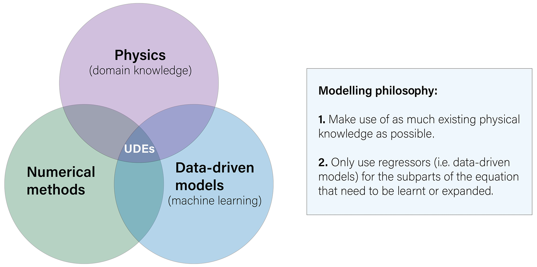
Figure 1Basic representation of universal differential equations (UDEs) and their associated modelling philosophy. UDEs sit at the intersection of physical domain knowledge, represented by differential equations, numerical methods used to solve the differential equations and data-driven models, often represented as machine learning.
In glaciology, models have not escaped these general trends. As for machine learning in general, classification methods have been more popular than regression methods (e.g. Baumhoer et al., 2019; Mohajerani et al., 2019). Nonetheless, progress has been made with surrogate models for ice flow modelling (Riel et al., 2021; Jouvet et al., 2021), subglacial processes (Brinkerhoff et al., 2020), glacier mass balance modelling (Bolibar et al., 2020a, b; Anilkumar et al., 2023; Guidicelli et al., 2023) or super-resolution applications to downscale glacier ice thickness (Leong and Horgan, 2020). In terms of modelling glacier processes regionally or globally, it is still very challenging to move from small-scale detailed observations and physical processes to large-scale observations and parametrizations. When modelling glaciers globally, simple empirical models such as temperature-index models are used due to their robustness to noise and the lack of observations needed to support more complex models. The same applies for ice flow dynamics, with flowline models based on the shallow-ice approximation (SIA; Hutter, 1983) being widely used, as it provides a good approximation, particularly with noisy and coarse-resolution input data typical of large-scale models (Maussion et al., 2019; Zekollari et al., 2019). Moreover, it also helps to reduce the computational cost of simulations with respect to higher-order models. Therefore, there is a broad need for new methods enabling a robust calibration and discovery of more sophisticated, nonlinear interpretable parametrizations in geosciences in general but also for both glacier mass balance and ice flow dynamics. These include the need to transition towards non-constant melt and accumulation factors for temperature-index mass balance models (Bolibar et al., 2022) or the need to find a robust relationship to calibrate ice creep and basal sliding for different regions, topographies and climates (Hock et al., 2023).
In terms of data assimilation and model parameter calibration, many different approaches to obtain differentiable glacier models have been developed (MacAyeal, 1993; Goldberg and Heimbach, 2013; Brinkerhoff et al., 2016). These inverse modelling frameworks enable the minimization of a loss function by finding the optimal values of parameters via their gradients. Such gradients can be found by either computing the associated adjoint or by using AD. Nonetheless, all efforts so far have been applied to the inversion of scalar parameters and sometimes their distributions (in the context of Bayesian inference), i.e. parameters that are stationary for a single inversion given a dataset. This means that the potential of learning the underlying physical processes is reduced to the current structure of the mechanistic model. No changes are made to the equations themselves, with the main role of the inversions being the fitting of one or more parameters already present in the equations. To advance beyond scalar parameter inversions, more complex inversions are required, shifting towards functional inversions. Functional inversions enable the capture of relationships between a parameter of interest and other proxy variables, resulting in a function that can serve as a law or parametrization. These learnt functions can then be added in the currently existing equation, thus expanding the underlying model with new knowledge.
We present an application of universal differential equations, i.e. a differential equation with an embedded function approximator (e.g. a neural network). For the purpose of this study, this NN is used to infer a prescribed artificial law determining the ice creep coefficient in Glen's law (Cuffey and Paterson, 2010) based on a climate proxy. Instead of treating it as a classic inverse problem, where a global parameter is optimized for a given point in space and time, neural networks learn a nonlinear function that captures the spatiotemporal variability in that parameter. This opens the door to a new way of learning parametrizations and empirical laws of physical processes from data. This case study is based on ODINN.jl v0.2 (Bolibar and Sapienza, 2023), a new open-source Julia package, available on GitHub at https://github.com/ODINN-SciML/ODINN.jl (last access: 13 June 2023). With this study, we attempt to share and discuss what the main advances and difficulties in applying UDEs to more complex physical problems are, we assess the current state of differentiable physics in Julia, and we suggest and project the next steps in order to scale this modelling framework to work with large-scale remote sensing datasets.
In this section we introduce the partial differential equation (PDE) describing the flow of ice through the SIA equation, and we present its equivalent universal differential equation (UDE) with an embedded neural network.
2.1 Glacier ice flow modelling
We consider the SIA equation to describe the temporal variation in the ice thickness (Cuffey and Paterson, 2010). Assuming a small depth-to-width ratio in ice thickness and that the driving stress caused by gravity is only balanced by the basal resistance, the evolution of the ice thickness can be described as a diffusion equation,
where n and A are the creep exponent and parameter in Glen's law, respectively; is the surface mass balance (SMB); C is a basal sliding coefficient; and ∇S is the gradient of the glacier surface , with B(x,y) being the bedrock elevation, and denotes its Euclidean norm.1 A convenient simplification of the SIA equation is to assume C=0, which implies a basal velocity equal to 0 all along the bed. This is reasonable when large portions of the glacier bed experience minimal sliding. In that case, Eq. (1) of the SIA can be written in the compact form
where D stands for an effective diffusivity given by
Except for a few engineered initial glacier conditions, no analytical solutions for the SIA equation exist, and it is necessary to use numerical methods (Halfar, 1981).
Importantly for our analysis, some of the coefficients that play a central role in the ice flow dynamics of a glacier (e.g. A, n and C) are generally non-constant and may vary both temporally and spatially. Although it is usually assumed that n≈3, this number can vary between 1.5 and 4.2 for different ice and stress configurations. Furthermore, the viscosity of the ice and consequently the Glen parameter A are affected by multiple factors, including ice temperature, pressure, water content and ice fabric (Cuffey and Paterson, 2010). For example, ice is harder and therefore more resistant to deformation at lower temperatures. The parameters A, n and C are usually used as tuning parameters and may or may not vary between glaciers depending on the calibration strategy and data availability.
An important property of the SIA equation is that the ice surface velocity u can be directly derived from the ice thickness H by the equation
Notice that the velocity field is a two-dimensional vector field that can be evaluated at any point in the glacier and points to the maximum direction of decrease in surface slope.
2.2 Universal differential equations
In the last few years there has been an increasing interest in transitioning physical models to a data-driven domain, where unknowns in the laws governing the physical system of interest are identified via the use of machine learning algorithms. The philosophy behind universal differential equations is to embed a rich family of parametric functions inside a differential equation so that the base structure of the differential equation is preserved, but more flexibility is allowed in the model at the moment of fitting observed data. This family of functions, usually referred to as the universal approximator because of their ability to approximate a large family of functions, includes, among others, neural networks, polynomial expansions and splines. An example of this is a universal ordinary differential equation (Rackauckas et al., 2020):
where f is a known function that describes the dynamics of the system, and Uθ(u,t) represents the universal approximator, a function parametrized by a vector parameter θ that takes as an argument the solution u and time t, as well as other parameters of interest, to the physical system.
In this study, the function f to be simulated is the SIA (Eq. 2). Training such a UDE requires that we optimize with respect to the solutions of the SIA equation, which needs to be solved using sophisticated numerical methods. The approach to fit the value of θ is to minimize the squared error between the target ice surface velocity profile (described in Sect. 3.1 together with all other datasets used) at a given time and the predicted surface velocities using the UDE, an approach known as trajectory matching (Ramsay and Hooker, 2017). For a single glacier, if we observed two different ice surface velocities u0 and u1 at times t0 and t1, respectively, then we want to find θ that minimizes the discrepancy between u1 and , defined as the forward numerical solution of the SIA equation yielding a surface ice velocity field following Eq. (4). When training with multiple glaciers, we are instead interested in minimizing the total level of agreement between observation and predictions,
where denotes the Frobenius norm, that is, the square root of the sum of the squares of all matrix entries, and each k corresponds to a different glacier. The weights ωk are included in order to balance the contribution of each glacier to the total loss function. For our experiments, we consider , which results in a rescaling of the surface velocities. This scaling is similar to the methods suggested in Kim et al. (2021) to improve the training of stiff neural ODEs.
2.3 Functional inversion
We consider a simple synthetic example where we fix n=3, a common assumption in glaciology; C=0; and model the dependency of Glen's creep parameter A and the climate temperature normal Ts, i.e. the average long-term variability in air temperature at the glacier surface. Ts is computed using a 30-year rolling mean of the air temperature series, used to drive the changes in A in the prescribed artificial law. Although simplistic and incomplete, this relationship allows us to present all of our methodological steps in the process of identifying more general phenomenological laws for glacier dynamics. Any other proxies of interest could be used instead of Ts for the design of the model. Instead of considering that the diffusivity Dθ is the output of a universal approximator, we replace the creep parameter A in Eq. (3) with a neural network with input Ts:
In this last equation, Dθ(Ts) parametrized using the neural network Aθ(Ts) plays the role of Uθ in Eq. (5), allowing the solutions of the PDE to span over a rich set of possible solutions. The objective of Aθ(Ts) will be to learn the spatial variability (i.e. among glaciers) in A with respect to Ts for multiple glaciers in different climates. In order to generate this artificial law, we have used the relationship between ice temperature and A from Cuffey and Paterson (2010) and replaced ice temperatures with a relationship between A and Ts. This relationship is based on the hypothesis that Ts is a proxy of ice temperature and therefore of A. However, it ignores many other important physical drivers influencing the value of A, such as a direct relationship with the temperature of ice, the type of fabric and the water content (Cuffey and Paterson, 2010). Nonetheless, this simple example serves to illustrate the modelling framework based on UDEs for glacier ice flow modelling while acting as a platform to present both the technical challenges and the adaptations performed in the process, as well as the future perspectives for applications at larger scales with additional data. Given this artificial law for A(Ts), a reference dataset of velocities and ice thicknesses is generated by solving Eq. (2) of the SIA.
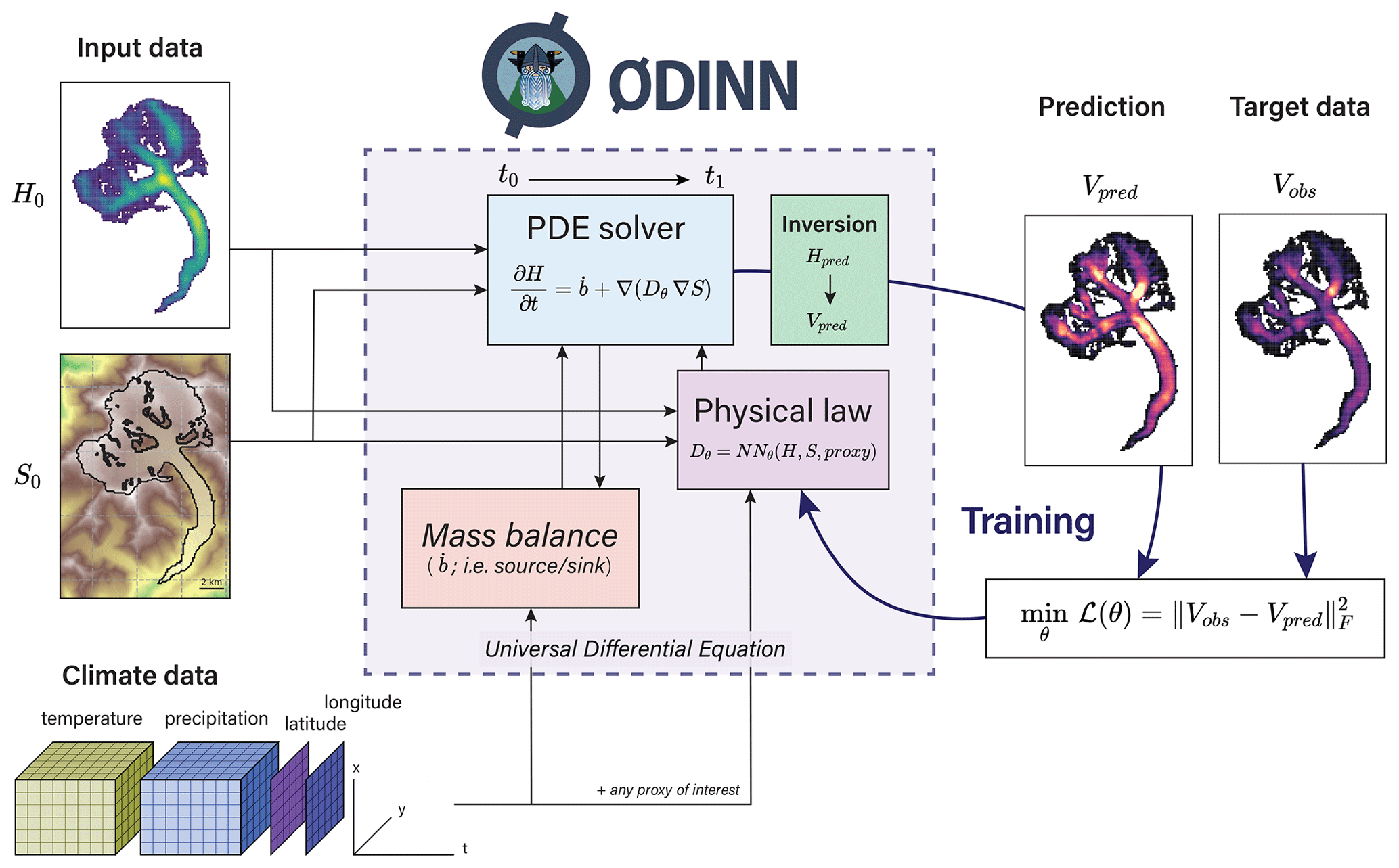
Figure 2Overview of ODINN.jl's workflow to perform functional inversions of glacier physical processes using universal differential equations. The parameters (θ) of a function determining a given physical process (Dθ), expressed by a neural network NNθ, are optimized in order to minimize a loss function. For this study, the physical law was constrained only by climate data, but any other proxies of interest can be used to design it. The glacier surface mass balance is downscaled (i.e. it depends) on S, which is updated by the solver, thus dynamically updating the state of the simulation for a given time step.
The combination of Python tools from the Open Global Glacier Model (OGGM) with the UDE glacier modelling framework in Julia has resulted in the creation of a new Julia package named ODINN.jl (OGGM + DIfferential equation Neural Networks; Bolibar and Sapienza, 2023). For the purpose of this study, ODINN has been used to study the viability of UDEs to solve and learn subparts of the SIA equation. The use of PyCall.jl enables a seamless integration of Python libraries such as OGGM and xarray (Hoyer and Hamman, 2017) within ODINN.
3.1 Training dataset
The following data are used for the initial conditions of simulated glaciers: a digital elevation model (DEM) for the glacier surface elevation S based on the Shuttle Radar Topography Mission from the year 2005 (SRTM; Farr et al., 2007) and estimated glacier ice thickness H from the global dataset from Farinotti et al. (2019) based on the glacier outlines around the year 2003 of the Randolph Glacier Inventory (Consortium, 2017). All these datasets, together with all glacier information, are retrieved using the Open Global Glacier Model (OGGM), an open-source glacier evolution model in Python providing a vast set of tools to retrieve and process climate and topographical data related to glaciers (Maussion et al., 2019). Since these datasets are only available for just one or a few times but have a global spatial coverage of almost all of the ∼ 220 000 glaciers on Earth, we perform this training for 17 different glaciers (see table in Appendix C) distributed in different climates around the world. This enables a good sampling of different climate conditions from which to take Ts to compute A. All climate data were based on the W5E5 climate dataset (Lange, 2019), also retrieved using OGGM. For the purpose of the synthetic experiments, some of the boundary conditions (surface topography, glacier bedrock inferred from topography and ice thickness) are assumed to be perfectly known.
3.2 Differential equation solver
In order to solve Eq. (2) of the SIA, we perform a discretization in the spatial domain to solve the problem as a combination of ordinary differential equations (ODEs). The solution of the ODEs is evaluated in a constant grid, determined by the preprocessed datasets by OGGM. The resolution of the spatial grid is automatically adjusted depending on the glacier size and domain size, typically ranging between 100×100 and 200×200 grid points, which leads to a system of coupled ODEs ranging from 10 000 to 40 000 equations per glacier. All gradients and divergences are computed in a staggered grid to improve stability (see Appendix A). Once the problem has been discretized in the spatial domain, we use the numerical solver RDPK3Sp35 (Ranocha et al., 2022) implemented in DifferentialEquations.jl (Rackauckas and Nie, 2017) to solve the SIA forward in time. The method implements an adaptive temporal step size close to the maximum value satisfying the CFL conditions for numerical stability at the same time that it controls numerical error and computational storage (Ranocha et al., 2022).
In order to create conditions similar to those one would encounter when using remote sensing observations for the functional inversions, we add Gaussian noise with a mean of 0 and standard deviation of (around 30 % of the average A value) to the output of the prescribed law (Fig. 3). This setup is used to compute the reference synthetic solutions ( in Eq. 6), which will then be used by the UDE to attempt to infer the prescribed law indirectly from glacier ice surface velocities and/or ice thickness.
For the SIA UDE, we substitute A by a small feed-forward neural network using Flux.jl (Innes et al., 2018). The architecture of the neural network consists of one single input variable; three hidden layers with 3, 10, and 3 units, respectively; and one single output variable. Since the optimization problem is much more constrained by the structure of the solutions of the PDE compared to a pure data-driven approach (Rackauckas et al., 2020), a very small neural network is enough to learn the dynamics related to the subpart of the equation it is representing (i.e. A). This network has a single input and output neuron, thus producing a one-to-one mapping. This small size is one of the main advantages of UDEs, which do not require as much data as traditional data-driven machine learning approaches. We use a softplus activation function in all layers except for the last layer, for which we use a rescaled sigmoid activation function which constrains the output within physically plausible values (i.e. 8−20 to 8−17 yr−1 Pa−3). Constraining the output values of the neural network is necessary in order to avoid numerical instabilities in the solver or very small step sizes in the forward model that will lead to expensive computations of the gradient. The use of continuous activation functions has been proven to be more effective for neural differential equations, since their derivatives are also smooth, thus avoiding problems of vanishing gradients (Kim et al., 2021).
3.3 Surface mass balance
In order to compute the glacier surface mass balance (i.e. a source/sink) for both the PDEs and the UDEs, we used a very simple temperature-index model with a single melt factor and a precipitation factor set to 5 mm d−1 ∘C−1 and 1.2, respectively. These are average values found in the literature (Hock, 2003), and despite its simplicity, this approach serves to add a realistic SMB signal on top of the ice rheology in order to assess the performance of the inversion method under realistic conditions. In order to add the surface mass balance term in Eq. (2) of the SIA, we used a DiscreteCallback from DifferentialEquations.jl. This enabled the modification of the glacier ice thickness H with any desired time intervals and without producing numerical instabilities when using all the numerical solvers available in the package (Rackauckas and Nie, 2017). We observed this makes the solution more stable without the need for reducing the step size of the solver.
In order to find a good compromise between computational efficiency and memory usage, we preprocess raw climate files from W5E5 (Lange, 2019) for the simulation period of each glacier. Then, within the run, for each desired time step where the surface mass balance needs to be computed (monthly by default), we read the raw climate file for a given glacier, and we downscale the air temperature to the current surface elevation S of the glacier given by the SIA PDE. For that, we use the adaptive lapse rates given by W5E5, thus capturing the topographical feedback of retreating glaciers in the surface mass balance signal (Bolibar et al., 2022).
3.4 Sensitivity methods and differentiation
In order to minimize the loss function from Eq. (6), we need to evaluate its gradient with respect to the parameters of the neural network and then perform gradient-based optimization. Different methods exist to evaluate the sensitivity or gradients of the solution of a differential equation. These can be classified depending on if they run backward or forward with respect to the solver. Furthermore, they can be divided between continuous and discrete, depending on if they manipulate a discrete evaluation of the solver or if instead they solve an alternative system of differential equations in order to find the gradients (see Fig. B1). For a more detailed overview on this topic, see Appendix B.
Here we compare the evaluation of the gradients using a continuous adjoint method integrated with automatic differentiation and a hybrid method that combines automatic differentiation with finite differences.
3.4.1 Continuous adjoint sensitivity analysis
For the first method based on pure automatic differentiation, we used the SciMLSensitivity.jl package, an evolution of the former DiffEqFlux.jl Julia package (Rackauckas et al., 2019), capable of weaving neural networks and differential equation solvers with AD. In order to train the SIA UDE from Eq. (7), we use the same previously mentioned numerical scheme as for the PDE (i.e. RDPK3Sp35). Unlike in the original neural ODEs paper (Chen et al., 2019), simply reversing the ODE for the backward solve results in unstable gradients. This has been shown to be the case for most differential equations, particularly stiff ones like the one from this study (Kim et al., 2021). In order to overcome this issue, we used the full solution of the forward pass to ensure stability during the backward solve, using the InterpolatingAdjoint method as described in the stiff neural ODEs paper (Kim et al., 2021). This method combined with an explicit solver proved to be more efficient than using a quadrature adjoint. It is also possible to use checkpointing and just store a few evaluations of the solution. This has the advantage of reducing memory usage at the cost of sacrificing some computational performance (Schanen et al., 2023; Griewank and Walther, 2008). To compute the vector Jacobian products involved in the adjoint calculations of the SIA UDE, we used reverse-mode AD with the ReverseDiff.jl package with a cached compilation of the reverse tape. We found that for our problem, the limitation of not being able to use control flow was easily bypassed, and performance was noticeably faster than other AD packages in Julia, such as Zygote.jl.
3.4.2 Finite differences
The second method consists of using AD just for the neural network and finite differences for capturing the variability in the loss function with respect to the parameter A. Notice that in Eq. (6) we can write ℒk(θ)=ℒk(Aθ(Tk)), with A(θ) being the function that maps input parameters Tk into the scalar value of A (which for this example is assumed to be a single scalar across the glacier) as a function of the neural network parameters θ. Once A has been specified, the function ℒk is a one-to-one function that is easily differentiable using finite differences. If we define g=∇θA(Tk) as the gradient of the neural network that we obtain using AD, then the full gradient of the loss function can be evaluated using the centred numerical approximation
where η is the step size used for the numerical approximation of the derivative. Notice that the first term on the right-hand side is just a scalar that quantifies the sign and amplitude of the gradient, which will always be in the direction of ∇θA(Tk). The choice of step size η is critical in order to correctly estimate the gradient. Notice that this method only works when there are a few parameters and will not generalize well to the case of an A that varies in space and time for each glacier. The main advantage of this method is that it runs orders of magnitude faster than a pure AD one.
3.5 Optimization
Once the gradient has been computed by one of the previous methods, optimization of the total loss function without any extra regularization penalty to the weights in the loss function is performed using a Broyden–Fletcher–Goldfarb–Shanno (BFGS) optimizer with parameter 0.001. We also tested ADAM (Mogensen and Riseth, 2018) with a learning rate of 0.01. BFGS converges in fewer epochs than ADAM, but it has a higher computational cost per epoch. Overall, BFGS performed better in different scenarios, resulting in a more reliable UDE training. For this toy model, a full epoch was trained in parallel using 17 workers, each one for a single glacier. Larger simulations will require batching either across glaciers or across time in the case that a dataset with dense temporal series are used.
3.6 Scientific computing in the cloud
In recent years, scientific workflows in Earth and environmental sciences have benefited from transitioning from local to cloud computing (Gentemann et al., 2021; Abernathey et al., 2021; Mesnard and Barba, 2020). The adoption of cloud computing facilitates the creation of shared computational environments, datasets and analysis pipelines, which leads to more reproducible scientific results by enabling standalone software containers (e.g. Binder, Project Jupyter et al., 2018) for other researchers to easily reproduce scientific results. As part of this new approach in terms of geoscientific computing, we are computing everything directly in the cloud using a JupyterHub (Granger and Pérez, 2021). This JupyterHub allows us to work with both Julia and Python, using Unix terminals, Jupyter notebooks (Thomas et al., 2016) and Visual Studio Code directly on the browser. Moreover, this provides a lot of flexibility in terms of computational resources. When logging in, one can choose between different machines, ranging from small ones (1–4 CPUs, 4–16 GB RAM) to very large ones (64 CPUs, 1 T4 tensor core GPU, 1 TB RAM), depending on the task to be run. The largest simulations for this study were run in a large machine, with 16 CPUs and 64 GB of RAM.
Despite its apparent simplicity, it is not a straightforward problem to invert the spatial function of A with respect to the predictor indirectly from surface velocities, mainly due to the highly nonlinear behaviour of the diffusivity of ice (see Eq. 2). We ran a functional inversion using two different differentiation methods for 17 different glaciers (see Table C1) for a period of 5 years.
Training the UDE with full batches using the continuous adjoint method described in Appendix B2 converges in around 20 epochs. The NN is capable of successfully approximating the prescribed nonlinear function of A. The loss sees a steep decrease in the first epochs, with BFGS optimizing the function towards the lowest values of A, which correctly approximate the majority of values of the prescribed nonlinear function. From this point, the function slowly converges until it finds an optimal non-overfitted solution (Fig. 3b). This simulation took about 3 h to converge, with a running time of between 6 to 12 min per epoch, in a machine in the cloud-based JupyterHub with 16 CPUs and 64 GB of RAM, using all available CPUs to simulate in parallel the 17 glaciers in batches and using the full 64 GB of memory. Figure 3a shows the parametrization of A as a function of Ts obtained with the trained NN. We observe that the neural network is able to capture the monotonic increasing function A(Ts) without overfitting the noisy values used for training (dots in the plot). Interestingly, the lack of regularization did not affect overfitting. We are unsure about the reasons behind this behaviour, but we suspect this could be related to an implicit regularization caused by UDEs. This property has not been studied yet, so more investigations should be carried out in order to better understand this apparent robustness to overfitting.
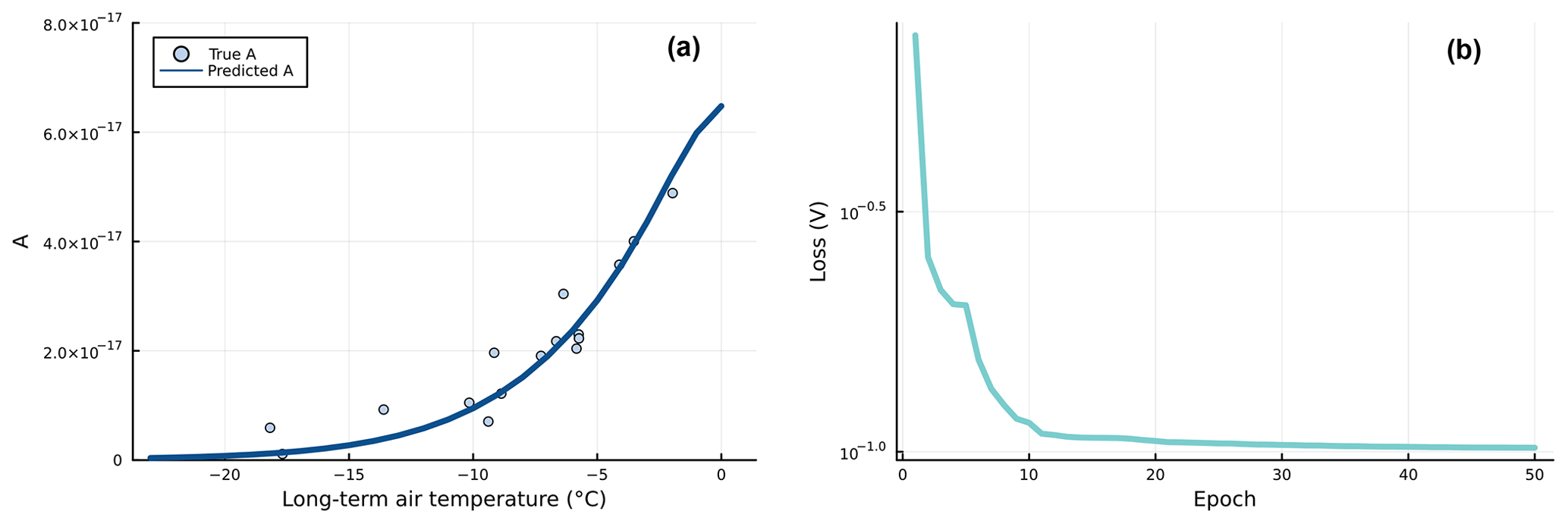
Figure 3(a) Inferred function by the NN embedded in the SIA PDE using full automatic differentiation. The NN learnt the prescribed noisy function (each dot represents a glacier), which relates Glen's coefficient A with a proxy of interest (i.e. the long-term air temperature Ts). (b) Evolution of the loss through training, using a BFGS optimizer. The loss is based on a scaled mean squared error in the difference between the simulated and target ice surface velocities. The scaling is used to correctly account for values of different orders of magnitude. Without any use of regularization, the optimization converges in around 20 epochs. Note that the loss is shown in log scale.
We also compared the efficiency of our approach when using the finite-difference scheme. Since this does not require heavy backward operations as the continuous adjoint method does, the finite-difference method runs faster (around 1 min per epoch). However, we encountered difficulties in picking the right step size η in Eq. (8). Small values of η lead to floating number arithmetic errors and large η to biased estimates of the gradient. On top of this effect, we found that numerical precision errors in the solution of the differential equation result in wrong gradients and the consequent failure in the optimization procedure (see discussion about this in Sect. 5.2.3). A solution for this would be to pick η adaptive as we update the value of the parameter θ. However, this would lead to more evaluations of the loss function. Instead, we applied early stopping when we observed that the loss function reached a reasonable minimum.
4.1 Robustness to noise in observations
The addition of surface mass balance (i.e. a source/sink) to the SIA equation further complicates things for the functional inversion, particularly from a computational point of view. The accumulation and ablation (subtraction) of mass on the glacier introduces additional noise to the pure ice flow signal. The mass loss in the lower elevations of the glacier slows down ice flow near the tongue, whereas the accumulation of mass in the higher elevations accelerates the ice flow on the upper parts of the glacier.
As an experiment to test the robustness of the functional inversions made by the UDE, we used different surface mass balance models for the reference simulation (i.e. the ground truth) and the UDE. This means that the surface mass balance signal during training is totally different from the one in the ground truth. We achieved this by using a temperature-index model with a melt factor of 4 mm d−1 ∘C−1 and a precipitation factor of 2 for the reference run, as well as a melt factor of 8 mm d−1 ∘C−1 and a precipitation factor of 1 for the UDE. This means that the UDE is perceiving a much more negative surface mass balance than the actual one from the ground truth. Despite the really large difference that can be seen in Fig. 4, the UDE was perfectly capable of inverting the nonlinear function of A. The evolution of the loss was less smooth than for the case of matching surface mass balance rates, but it also converged in around 20 epochs, with no noticeable difference in final performance.
This shows the robustness of this modelling approach, particularly when the ice surface velocities u are used in the loss function. Unlike the glacier ice thickness, u is much less sensitive to changes in surface elevation, making it a perfect datum for inferring ice rheology properties. This is also due to the fact that we are using ice surface velocities averaged across multiple years, which lessen the importance of changes in surface elevation. When working with velocities with a higher temporal resolution, these will likely become more sensitive to noise. This weak dependence on the surface mass balance signal will be highly beneficial for many applications, since it will imply that the inversion can be done even if we only have an approximate representation of the surface mass balance, which will be the case for many glaciers. Various tests using H instead of u as the target data showed that A cannot be successfully inverted in the presence of a surface mass balance signal.
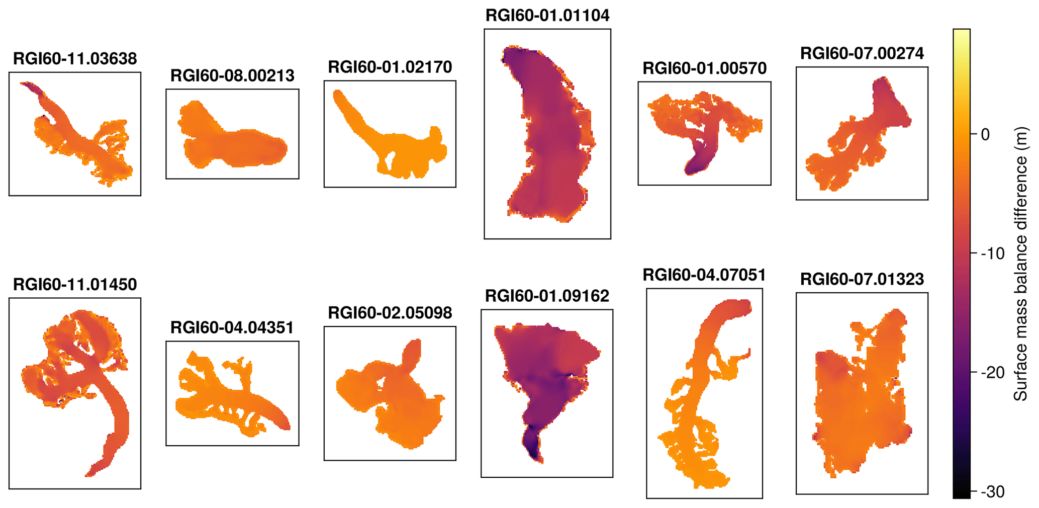
Figure 4Differences in surface elevation for a 5-year simulation, coming from the different applied surface mass balance rates, between the ground truth data and the training of the UDE. Despite the noise coming from the different surface mass balance signals, the UDE is perfectly capable of learning the underlying nonlinear function of A. This proves the robustness against noise of this functional inversion framework for glacier rheology when using ice surface velocities. Only 12 of the total of 17 glaciers are shown.
5.1 Application to functional inversions of glacier physical processes
This first implementation of a UDE on glacier ice flow modelling serves as a baseline to tackle more complex problems with large datasets. One main simplification of this current setup needs to be overcome in order to make the model useful at a global scale for exploring and discovering empirical laws. In this study, only ice deformation (creep) has been taken into account in the diffusivity. Basal sliding, at the ice–bedrock interface, will have to be included in the SIA equation to accommodate different configurations and behaviours of many glaciers around the world. Therefore, a logical next step would be to infer D in Eq. (3), including the sliding coefficient C from Eq. (2) using a UDE. Nonetheless, despite a scale difference between these two processes, this can be an ill-posed problem, since the only available ice velocity observations are from the surface, encompassing both creep and basal sliding. This results in degeneracy (i.e. equifinality), making it very challenging to disentangle the contributions of each physical process to ice flow. This is particularly true for datasets with average annual surface velocities, since both physical processes contribute to glacier velocities, with no obvious way of separating them. In order to overcome such issues, using new remote sensing datasets with high temporal resolution, like Nanni et al. (2023) with observations every 10 d, can help to better constrain the contribution of each physical process. This implies that we can exploit not only the spatial dimension with multiple glaciers, but also rich time series of the fluctuations in glacier velocities along the seasons. Such dynamics can help disentangle the main contributions of creep during the winter season and the onset of sliding during the summer season as the subglacial hydrological network activates due to melt.
Interestingly, depending on the ice surface velocity observations used, the need for a numerical solver and a UDE is not imperative for a functional inversion. For a single snapshot of ice surface velocities between two dates (e.g. 2017–2018 in Millan et al., 2022), a functional inversion can be performed directly on the SIA equation without the need for a solver. The average ice surface velocities can be directly inverted if the geometry is known. This reduces the technical complexity enormously, enabling one to focus on more complex NN architectures and functions to inverse ice rheology and basal sliding properties. Some initial tests have shown that such problems train orders of magnitude faster. However, since only one timestamp is present for the inversions, the inversion is extremely sensitive to time discrepancies in the input datasets, making it potentially quite vulnerable to noisy or temporally misaligned datasets.
Alternatively, the optimization of the NN for ice rheology inference based on ice surface velocities has proved to be robust to the noise added by the SMB component. This serves to validate an alternative glacier ice dynamic model calibration strategy to that of the majority of large-scale glacier models (e.g. OGGM and GloGEM; Huss and Hock, 2015). By being able to calibrate ice rheology and mass balance (MB) separately, one can avoid many equifinality problems that appear when attempting to calibrate both components at the same time (Arthern and Gudmundsson, 2010; Zhao et al., 2018). A classic problem of a joint calibration is the ambiguity in increasing/decreasing accumulation vs increasing/decreasing Glen's coefficient (A). ODINN.jl, with its fully differentiable code base, provides a different strategy consisting of two main steps: (i) calibrating the ice rheology from observed ice surface velocities (Millan et al., 2022), observed ice thicknesses (GlaThiDa Consortium Consortium, 2019) and DEMs and (ii) calibrating the MB component (e.g. melt and accumulation factors) with the previously calibrated ice rheology based on both point glaciological MB observations and multiannual geodetic MB observations (Hugonnet et al., 2020). This maximizes the use of current glaciological datasets for model calibration, even for transient simulations. Such a differentiable modelling framework presents both the advantages of complex inversions and the possibility of performing data assimilation with heterogeneous and sparse observations.
5.2 Scientific machine learning
5.2.1 Automatic differentiation approaches
Automatic differentiation is the centrepiece of the modelling framework presented in this study. In the Julia programming language, multiple AD packages exist, which are compatible with both differential equation and neural network packages, as part of the SciML ecosystem. Each package has advantages and disadvantages, which make them suitable for different tasks. In our case, ReverseDiff.jl turned out to be the best-performing AD package due to the speed gained by reverse tape compilation. Together with Zygote.jl (Innes et al., 2019), another popular backward AD package, they have the limitation of not allowing mutation of arrays. This implies that no in-place operations can be used, thus augmenting the memory allocation of the simulations considerably. Enzyme.jl (Moses et al., 2021) is arising as a promising alternative, with the fastest gradient computation times in Julia (Ma et al., 2021). It directly computes gradients on statically analysable LLVMs, without differentiating any Julia source code. Nonetheless, Enzyme.jl is still under heavy development, and it is still not stable enough for problems like the ones from this study. As Enzyme.jl will become more robust in the future, it appears likely to become the de facto solution for AD in Julia.
Overall, the vision on AD from Julia is highly ambitious, attempting to perform AD directly on source code, with minimal impact on the user side and with the possibility of easily switching AD back ends. From a technical point of view, this is much more complex to achieve than hard-coded gradients linked to specific operators, an approach followed by JAX (Bradbury et al., 2020) and other popular deep learning Python libraries. In the short term, the latter provides a more stable experience, albeit a more rigid one. However, in the long term, once these packages are given the time to grow and become more stable, differentiating through complex code, like the one from UDEs, they should become increasingly straightforward.
5.2.2 Replacing the numerical solver with a statistical emulator
In this work, we model glacier ice flow using a two-dimensional SIA equation described by Eq. (2). This decision was originally driven by the goal of using a differential equation that is general enough for modelling the gridded remote sensing available data but also flexible enough to include unknowns in the equation in both the diffusivity and the surface mass balance terms. Nonetheless, the approach of UDEs and functional inversions is flexible and can be applied to more complex ice flow models, such as full-Stokes. It is important to keep in mind that for such more complex models, the numerical solvers involved would be computationally more expensive to run, in both forward and reverse mode.
A recent alternative to such a computationally heavy approach is the use of convolutional neural networks as emulators for the solutions of the differential equations of a high-order ice flow model (Jouvet et al., 2021; Wang et al., 2022). Emulators can be used to replace the numerical solver shown in the workflow illustrated in Fig. 2 while keeping the functional inversion methodology intact. This in fact translates to replacing a numerical solver with a previously trained neural network, which has learnt to solve the Stokes equations for ice flow. Embedding a neural network inside a second neural network that gives approximate solutions instead of a PDE solved by a numerical solver allows for computing the full gradient of the loss function by just using reverse AD. Neural networks can very easily be differentiated, thus resulting in a simpler differentiation scheme. At the same time, as shown in Jouvet (2023), this could potentially speed up functional inversions by orders of magnitude while also improving the quality of the ice flow simulations transitioning from the SIA, with its vertically integrated ice column assumption, to full-Stokes.
5.2.3 New statistical questions
The combination of solvers for differential equations with modern machine learning techniques opens the door to new methodological questions that include the standard ones about the design of the machine learning method (loss function, optimization method, regularization) but also new phenomena that emerge purely by the use of numerical solutions of differential equations in the loss function. Although this intersection between data science and dynamical systems has been widely explored (see Ramsay and Hooker, 2017), the use of adjoints for sensitivity analysis integrated with AD tools for optimization and the properties of the landscape generated when using numerical solvers have not. Because numerical methods approximate the solution of the differential equation, there is an error term associated with running the forward model that can be amplified when running the model backward when computing the adjoint. This can lead to inaccurate gradients, especially for stiff differential equations (Kim et al., 2021). Furthermore, when computing a loss function that depends on the solution of the differential equation for a certain parameter θ, the loss depends on θ because local variations in θ result in changes in the error itself but also because of hyper-parameters in the numerical solver (for example, the time step used to ensure stability) that are adaptively selected as a function of θ. This double dependency of the loss as a function of θ results in distortions of the shape of the loss function (Creswell et al., 2023). Further investigation is needed in order to establish the effect of these distortions during optimization and how these can impact the calculation of the gradient obtained using different sensitivity methods.
Another interesting question pertains to the training and regularization of UDEs and related physics-informed neural networks. During training, we observed that the neural network never overfitted the noisy version of prescribed law A(Ts) (see Sect. 3.2). We conjecture that one reason why this may be happening is because of the implicit regularization imposed by the form of the differential equation in Eq. (2).
Despite the ever-increasing numbers of new Earth observations coming from remote sensing, it is still extremely challenging to translate complex, sparse, noisy data into actual models and physical laws. Paraphrasing Rackauckas et al. (2020), in the context of science, the well-known adage a picture is worth a thousand words might well be a model is worth a thousand datasets. Therefore, there is a clear need for new modelling frameworks capable of generating data-driven models with the interpretability and constraints of classic physical models. Universal differential equations (UDEs) embed a universal function approximator (e.g. a neural network) inside a differential equation. This enables additional flexibility typical of data-driven models into a reliable physical structure determined by a differential equation.
We presented ODINN.jl, a new modelling framework based on UDEs applied to glacier ice flow modelling. We illustrated how UDEs, supported by differentiable programming in the Julia programming language, can be used to retrieve empirical laws present in datasets, even in the presence of noise. We did so by using the shallow-ice approximation PDE and learning a prescribed artificial law as a subpart of the equation. We used a neural network to infer Glen's coefficient A, determining the ice viscosity, with respect to a climatic proxy for 17 different glaciers across the world. The presented functional inversion framework is robust to noise present in input observations, particularly with regard to the surface mass balance, as shown in an experiment.
This study can serve as a baseline for other researchers interested in applying UDEs to similar nonlinear diffusivity problems. It also provides a code base to be used as a backbone to explore new parametrizations for large-scale glacier modelling, such as for glacier ice rheology, basal sliding or more complex hybrid surface mass balance models.
Solving Eq. (2) is challenging since the diffusivity D depends on the solution H. Furthermore, the SIA equation is a degenerate diffusion equation since the diffusivity D vanishes as H→0 or ∇S→0. In cases where the glacier does not extend to the margins of our domain, this allows us to treat the SIA equation as a free-boundary problem (Fowler and Ng, 2020). However, at the moment of solving the differential equation with a numerical solver, we still need to impose the constraint that the ice thickness is non-negative, that is, H≥0.
We consider a uniform grid on points (xj,yk), with and , with . Starting from an initial time t0, we update the value of the solution for H by steps Δti, with . We refer to for the numerical approximation of . In this way, we have a system of ODEs for each Hj,k.
An important consideration when working with numerical schemes for differential equations is the stability of the method. Here we consider just explicit methods, although the spatial discretization is the same for implicit methods. Explicit methods for the SIA equation are conditionally stable. In order to get stability, we need to undertake the following (Fowler and Ng, 2020):
-
Evaluate the diffusivity in a staggered grid labelled by semi-integer indices (circles on the dotted grid in Fig. A1). This grid is closely related to Scheme E of Arakawa grids (Arakawa and Lamb, 1977).
-
Choose a temporal step size Δt such that , where Dmax is the maximum diffusivity.
The algorithm to solve the SIA equation follows the next steps:
-
Assume we know the value of at a given time ti. Then, we compute all the diffusivities on the staggered grid. As we mentioned before, the diffusivity is a function of H, and . Instead of using one single estimate of H to approximate all these quantities, the idea is to use average quantities on the primal grid to compute the diffusivity on the staggered grid (red arrows in Fig. A1). We define the average quantities as
Then, we compute the diffusivity on the staggered grid as
-
Compute (another) average diffusivity but now on the edges of the primal grid (blue arrows in Figure A1):
-
Compute the diffusive part of the SIA equations on the point in the primal grid (j,k) as
-
Update the value of H following an explicit scheme. Here we use the different solvers available in
DifferentialEquations.jl. Just for illustration, a simple explicit scheme could be one that updates the values of the ice thickness followingwhere Δti is the time step, which in our case is automatically selected by the numerical solver to ensure stability.
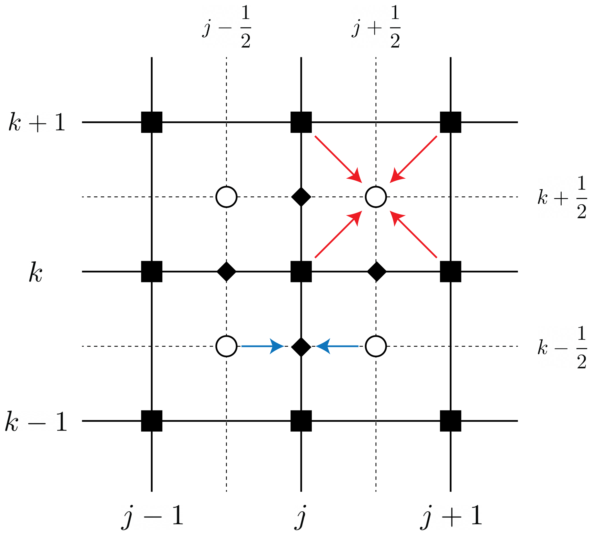
Figure A1Staggered grid used to solve the shallow-ice approximation PDE. The black squares represent the primal grid, empty circles the staggered grid, diamonds the points in the grid where the diffusivity evaluated in the staggered grid is averaged (Eqs. A5 and A6), blue arrows operations in the edges of the primal grid and red arrows operations in the staggered grid.
In practice, the step size Δti is chosen automatically by the numerical solver included in DifferentialEquations.jl (Rackauckas and Nie, 2017). However, this does not automatically guarantee that the updates in the ice thickness (Eq. A8) make . A sufficient condition is given by (Imhof, 2021)
This condition guarantees that the computed diffusivity (Eq. A7) satisfies
and hence
where the last inequality is a consequence of the stability condition . In cases where no mass balance term is added , we simply have that for all grid points. In the general case with mass balance, we still need to clip the updated ice thickness by replacing by . This includes the cases with excessive ablation.
In this section we provide a high-level explanation of the two methods we used to compute the gradient of functions involving solutions of differential equations, namely finite differences and continuous adjoint sensitivity analysis. Consider a system of ordinary differential equations given by
where u∈ℝn and θ∈ℝp. We are interested in computing the gradient of a given loss function with respect to the parameter θ.
B1 Finite differences
The simplest way of evaluating a derivative is by computing the difference between the evaluation of the function at a given point and a small perturbation of the function. In the case of a loss function, we can approximate
with ei being the ith canonical vector and ε a small number. Even better, it is easy to see that the centred difference scheme
also leads to a more precise estimation of the derivative.
However, there are a series of problems associated with this approach. The first one is how this scales with the number of parameters p. Each directional derivative requires the evaluation of the function twice. For the centred difference approach in Eq. (B3), this will require 2p function evaluations, which demand to solve the differential equation in forward mode each time. A second problem is due to truncation errors. Equation (B2) involves the subtraction of two numbers that are very close to each other. As ε gets smaller, this will lead to truncation of the subtraction, introducing numerical errors that then will be amplified by the division by ε. Due to this, some heuristics have been introduced in order to pick the value of ε that will minimize the error, specifically picking , with εmachine being the machine precision (e.g. Float64). However, in practice it is difficult to pick a value of ϵ that leads to universal good estimations of the gradient.
B2 Continuous adjoint sensitivity analysis (CASA)
Consider an integrated loss function of the form
which includes the simple case of the loss function ℒk(θ) in Eq. (6). Using the Lagrange multiplier trick, we can write a new loss function I(θ) identical to L(θ) as
where λ(t)∈ℝn is the Lagrange multiplier of the continuous constraint defined by the differential equation. Now,
We can derive an easier expression for the last term using integration by parts. We define the sensitivity as and then perform integration by parts in the term , where we derive
Now, we can force some of the terms in the last equation to be 0 by solving the following adjoint differential equation for λ(t)T in backward mode:
with the final condition being λ(t1)=0. Then, in order to compute the full gradient , we
-
solve the original differential equation ,
-
solve the backward adjoint differential equation Eq. (B8) and
-
compute the simplified version of the full gradient in Eq. (B7) as
In order to solve the adjoint equation, we need to know u(t) at any given time. There are different ways in which we can accomplish this: (i) we can again solve for u(t) backward, (ii) we can store u(t) in memory during the forward step, or (iii) we can do checkpointing to save some reference values in memory and use them to recompute the solution between them (Schanen et al., 2023). Computing the ODE backward can be unstable and can lead to exponential errors (Kim et al., 2021). In Chen et al. (2019), the solution is recalculated backward together with the adjoint simulating augmented dynamics. One way of solving this system of equations that ensures stability is by using implicit methods. However, this requires cubic time in the total number of ordinary differential equations, leading to a total complexity of 𝒪((n+p)3) for the adjoint method. Two alternatives are proposed in Kim et al. (2021): the first one called quadrature adjoint produces a high-order interpolation of the solution u(t) as we move forward, then solves for λ backward using an implicit solver and finally integrates in a forward step. This reduces the complexity to 𝒪(n3+p), where the cubic cost in the number of ODEs comes from the fact that we still need to solve the original stiff differential equation in the forward step. A second but similar approach is to use an implicit–explicit (IMEX) solver, where we use the implicit part for the original equation and the explicit for the adjoint. This method will also have the complexity 𝒪(n3+p).
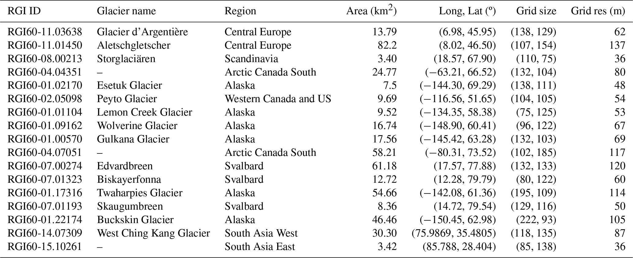
Table C1 includes all the details of the glaciers used in this study to train the UDE. Glaciers were picked randomly across the world to sample different climates with long-term air temperatures ranging from −20 ∘C to close to 0 ∘C. These data were retrieved using OGGM's preprocessing tools from the Randolph Glacier Inventory v6 (Consortium, 2017). Note that OGGM processes the necessary gridded data (i.e. DEMs, ice thickness data) in a constant adaptive grid, which depends on glacier size.
Table C1Table of glaciers used for training the UDE. Grid size and grid res (i.e. resolution) indicate the adaptive constant grid used by OGGM to adapt all gridded data for each glacier.
The source code of ODINN.jl v0.2.0 (Bolibar and Sapienza, 2023) used in this study is available as an open-source Julia package: https://github.com/ODINN-SciML/ODINN.jl (last access: 13 June 2023). The package includes continuous integration tests, installation guidelines on how to use the model and a Zenodo DOI: https://doi.org/10.5281/zenodo.8033313 (Bolibar and Sapienza, 2023). OGGM v1.6 (https://doi.org/10.5281/zenodo.7718476 Maussion et al., 2023) is also available as an open-source Python package at https://github.com/OGGM/oggm (last access: 10 March 2023), with documentation and tutorials available at https://oggm.org (last access: 13 June 2023).
JB conceived the project, designed the study, developed the model, wrote the paper and made the figures. FS designed the study, developed the model, investigated the sensitivity methods and wrote the paper. FM helped with retrieving the datasets to force the model with OGGM, contributed to the coupling between both models and provided glaciological advice. RL helped with the experiment design and technical choices. BW provided glaciological advice and helped design the project. FP provided advice on the methods and software development and helped design the project. All authors contributed to the writing of the paper by providing comments and feedback.
At least one of the (co-)authors is a member of the editorial board of Geoscientific Model Development. The peer-review process was guided by an independent editor, and the authors also have no other competing interests to declare.
Publisher's note: Copernicus Publications remains neutral with regard to jurisdictional claims made in the text, published maps, institutional affiliations, or any other geographical representation in this paper. While Copernicus Publications makes every effort to include appropriate place names, the final responsibility lies with the authors.
We would like to thank Kurt Cuffey for valuable discussions and comments on glacier modelling and physics; Harry Zekollari for all the conversations and help related to large-scale glacier modelling; Per-Olof Persson for the discussions on differential equations and numerical solvers; Giles Hooker for useful feedback regarding the statistical analysis; Chris Rackauckas for all the insights and discussions regarding scientific machine learning in the Julia ecosystem; and the Julia community for the technical support, bug hunting, and the interesting discussions in the Julia Slack and Discourse. We also thank the Jupyter Meets the Earth and 2i2c team (Erik Sundell, Yuvi Panda and many others) for helping with the infrastructure of the JupyterHub. Jordi Bolibar would like to thank CNRS – UGA, Institut des Géosciences de l'Environnement, UMR 5001, in Grenoble (France) for hosting him as an invited researcher. We thank Douglas Brinkerhoff and the anonymous reviewer for their constructive comments that helped improve the quality of this paper.
This research has been supported by the Nederlandse Organisatie voor Wetenschappelijk Onderzoek, Stichting voor de Technische Wetenschappen (Vidi grant 016.Vidi.171.063) and the National Science Foundation (EarthCube programme under awards 1928406 and 1928374).
This paper was edited by Ludovic Räss and reviewed by Douglas Brinkerhoff and one anonymous referee.
Abadi, M., Agarwal, A., Barham, P., Brevdo, E., Chen, Z., Citro, C., Corrado, G. S., Davis, A., Dean, J., Devin, M., Ghemawat, S., Goodfellow, I., Harp, A., Irving, G., Isard, M., Jia, Y., Jozefowicz, R., Kaiser, L., Kudlur, M., Levenberg, J., Mane, D., Monga, R., Moore, S., Murray, D., Olah, C., Schuster, M., Shlens, J., Steiner, B., Sutskever, I., Talwar, K., Tucker, P., Vanhoucke, V., Vasudevan, V., Viegas, F., Vinyals, O., Warden, P., Wattenberg, M., Wicke, M., Yu, Y., and Zheng, X.: TensorFlow: Large-Scale Machine Learning on Heterogeneous Distributed Systems, arXiv [preprint], https://doi.org/10.48550/arXiv.1603.04467, 2016. a
Abernathey, R. P., Augspurger, T., Banihirwe, A., Blackmon-Luca, C. C., Crone, T. J., Gentemann, C. L., Hamman, J. J., Henderson, N., Lepore, C., McCaie, T. A., Robinson, N. H., and Signell, R. P.: Cloud-Native Repositories for Big Scientific Data, Comput. Sci. Eng., 23, 26–35, https://doi.org/10.1109/MCSE.2021.3059437, 2021. a
Anilkumar, R., Bharti, R., Chutia, D., and Aggarwal, S. P.: Modelling point mass balance for the glaciers of the Central European Alps using machine learning techniques, The Cryosphere, 17, 2811–2828, https://doi.org/10.5194/tc-17-2811-2023, 2023. a
Arakawa, A. and Lamb, V. R.: Computational design of the basic dynamical processes of the UCLA general circulation model, General circulation models of the atmosphere, 17, 173–265, 1977. a
Arendt, A. A., Hamman, J., Rocklin, M., Tan, A., Fatland, D. R., Joughin, J., Gutmann, E. D., Setiawan, L., and Henderson, S. T.: Pangeo: Community tools for analysis of Earth Science Data in the Cloud, in: AGU Fall Meeting Abstracts, vol. 2018, IN54A–05, 2018. a
Arthern, R. J. and Gudmundsson, G. H.: Initialization of ice-sheet forecasts viewed as an inverse Robin problem, J. Glaciol., 56, 527–533, https://doi.org/10.3189/002214310792447699, 2010. a
Baumhoer, C. A., Dietz, A. J., Kneisel, C., and Kuenzer, C.: Automated Extraction of Antarctic Glacier and Ice Shelf Fronts from Sentinel-1 Imagery Using Deep Learning, Remote Sens., 11, 2529, https://doi.org/10.3390/rs11212529, 2019. a
Bezanson, J., Edelman, A., Karpinski, S., and Shah, V. B.: Julia: A Fresh Approach to Numerical Computing, SIAM Review, 59, 65–98, https://doi.org/10.1137/141000671, 2017. a, b
Bolibar, J. and Sapienza, F.: ODINN-SciML/ODINN.jl: v0.2.0, Zenodo [code], https://doi.org/10.5281/zenodo.8033313, 2023. a, b, c, d
Bolibar, J., Rabatel, A., Gouttevin, I., and Galiez, C.: A deep learning reconstruction of mass balance series for all glaciers in the French Alps: 1967–2015, Earth Syst. Sci. Data, 12, 1973–1983, https://doi.org/10.5194/essd-12-1973-2020, 2020a. a
Bolibar, J., Rabatel, A., Gouttevin, I., Galiez, C., Condom, T., and Sauquet, E.: Deep learning applied to glacier evolution modelling, The Cryosphere, 14, 565–584, https://doi.org/10.5194/tc-14-565-2020, 2020b. a
Bolibar, J., Rabatel, A., Gouttevin, I., Zekollari, H., and Galiez, C.: Nonlinear sensitivity of glacier mass balance to future climate change unveiled by deep learning, Nat. Commun., 13, 409, https://doi.org/10.1038/s41467-022-28033-0, 2022. a, b
Bradbury, J., Frostig, R., Hawkins, P., Johnson, M. J., Leary, C., Maclaurin, D., and Wanderman-Milne, S.: JAX: composable transformations of Python+ NumPy programs, 2018, Github [code], http://github.com/google/jax, 2020. a, b
Brinkerhoff, D., Aschwanden, A., and Fahnestock, M.: Constraining subglacial processes from surface velocity observations using surrogate-based Bayesian inference, J. Glaciol., 67, 385–403, https://doi.org/10.1017/jog.2020.112, 2021. a
Brinkerhoff, D. J., Meyer, C. R., Bueler, E., Truffer, M., and Bartholomaus, T. C.: Inversion of a glacier hydrology model, Ann. Glaciol., 57, 84–95, https://doi.org/10.1017/aog.2016.3, 2016. a
Chen, R. T. Q., Rubanova, Y., Bettencourt, J., and Duvenaud, D.: Neural Ordinary Differential Equations, arXiv [preprint], https://doi.org/10.48550/arXiv.1806.07366, 2019. a, b, c, d
Consortium, Randolph Glacier Inventory: Randolph Glacier Inventory 6.0, Consortium, RGI [data set], https://doi.org/10.7265/N5-RGI-60, 2017. a, b
Creswell, R., Shepherd, K. M., Lambert, B., Mirams, G. R., Lei, C. L., Tavener, S., Robinson, M., and Gavaghan, D. J.: Understanding the impact of numerical solvers on inference for differential equation models, arXiv [preprint], https://doi.org/10.48550/arXiv.2307.00749, 2023. a
Cuffey, K. and Paterson, W. S. B.: The physics of glaciers, Butterworth-Heinemann/Elsevier, Burlington, MA, 4th Edn., ISBN 978-0-12-369461-4, 2010. a, b, c, d, e
Farinotti, D., Huss, M., Fürst, J. J., Landmann, J., Machguth, H., Maussion, F., and Pandit, A.: A consensus estimate for the ice thickness distribution of all glaciers on Earth, Nat. Geosci., 12, 168–173, https://doi.org/10.1038/s41561-019-0300-3, 2019. a
Farr, T. G., Rosen, P. A., Caro, E., Crippen, R., Duren, R., Hensley, S., Kobrick, M., Paller, M., Rodriguez, E., Roth, L., Seal, D., Shaffer, S., Shimada, J., Umland, J., Werner, M., Oskin, M., Burbank, D., and Alsdorf, D.: The shuttle radar topography mission, Rev. Geophys., 45, RG2004, https://doi.org/10.1029/2005RG000183, 2007. a
Fowler, A. and Ng, F.: Glaciers and Ice Sheets in the climate system: The Karthaus summer school lecture notes, Springer, Nature, https://doi.org/10.1007/978-3-030-42584-5, 2020. a, b
Gentemann, C. L., Holdgraf, C., Abernathey, R., Crichton, D., Colliander, J., Kearns, E. J., Panda, Y., and Signell, R. P.: Science Storms the Cloud, AGU Advances, 2, 2, https://doi.org/10.1029/2020av000354, 2021. a
GlaThiDa Consortium: Glacier Thickness Database 3.1.0, World Glacier Monitoring Service [data set], Zurich, Switzerland, https://doi.org/10.5904/wgms-glathida-2020-10, 2019. a
Goldberg, D. N. and Heimbach, P.: Parameter and state estimation with a time-dependent adjoint marine ice sheet model, The Cryosphere, 7, 1659–1678, https://doi.org/10.5194/tc-7-1659-2013, 2013. a
Granger, B. E. and Pérez, F.: Jupyter: Thinking and Storytelling With Code and Data, Comput. Sci. Eng., 23, 7–14, https://doi.org/10.1109/MCSE.2021.3059263, 2021. a
Griewank, A. and Walther, A.: Evaluating Derivatives, Society for Industrial and Applied Mathematics, 2nd Edn., https://doi.org/10.1137/1.9780898717761, 2008. a
Guidicelli, M., Huss, M., Gabella, M., and Salzmann, N.: Spatio-temporal reconstruction of winter glacier mass balance in the Alps, Scandinavia, Central Asia and western Canada (1981–2019) using climate reanalyses and machine learning, The Cryosphere, 17, 977–1002, https://doi.org/10.5194/tc-17-977-2023, 2023. a
Halfar, P.: On the dynamics of the ice sheets, J. Geophys. Res.-Oceans, 86, 11065–11072, https://doi.org/10.1029/jc086ic11p11065, 1981. a
Hock, R.: Temperature index melt modelling in mountain areas, J. Hydrol., 282, 104–115, https://doi.org/10.1016/S0022-1694(03)00257-9, 2003. a
Hock, R., Maussion, F., Marzeion, B., and Nowicki, S.: What is the global glacier ice volume outside the ice sheets?, J. Glaciol., 69, 204–210, https://doi.org/10.1017/jog.2023.1, 2023. a
Hoyer, S. and Hamman, J. J.: xarray: N-D labeled Arrays and Datasets in Python, J. Open Res. Softw., 5, 10, https://doi.org/10.5334/jors.148, 2017. a
Hugonnet, R., McNabb, R., Berthier, E., Menounos, B., Nuth, C., Girod, L., Farinotti, D., Huss, M., Dussaillant, I., Brun, F., and Kääb, A.: A globally complete, spatially and temporally resolved estimate of glacier mass change: 2000 to 2019, EGU General Assembly 2020, Online, 4–8 May 2020, EGU2020-20908, https://doi.org/10.5194/egusphere-egu2020-20908, 2020. a, b
Huss, M. and Hock, R.: A new model for global glacier change and sea-level rise, Front. Earth Sci., 3, https://doi.org/10.3389/feart.2015.00054, 2015. a
Hutter, K.: Theoretical Glaciology, Springer Netherlands, Dordrecht, https://doi.org/10.1007/978-94-015-1167-4, 1983. a
Imhof, M. A.: Combined climate-ice flow modelling of the Alpine ice field during the Last Glacial Maximum, VAW-Mitteilungen, Doctoral thesis, 152 pp., https://doi.org/10.3929/ethz-b-000471073, 2021. a
Innes, M., Saba, E., Fischer, K., Gandhi, D., Rudilosso, M. C., Joy, N. M., Karmali, T., Pal, A., and Shah, V.: Fashionable Modelling with Flux, CoRR, ArXiv [preprint], https://doi.org/10.48550/arXiv.1811.01457, 2018. a
Innes, M., Edelman, A., Fischer, K., Rackauckas, C., Saba, E., Shah, V. B., and Tebbutt, W.: A Differentiable Programming System to Bridge Machine Learning and Scientific Computing, arXiv [preprint], https://doi.org/10.48550/arXiv.1907.07587, 2019. a
Jouvet, G.: Inversion of a Stokes glacier flow model emulated by deep learning, J. Glaciol., 69, 13–26, https://doi.org/10.1017/jog.2022.41, 2023. a
Jouvet, G., Cordonnier, G., Kim, B., Lüthi, M., Vieli, A., and Aschwanden, A.: Deep learning speeds up ice flow modelling by several orders of magnitude, J. Glaciol., 68, 651–664, https://doi.org/10.1017/jog.2021.120, 2021. a, b, c
Kidger, P.: On Neural Differential Equations, arXiv [preprint], https://doi.org/10.48550/arXiv.2202.02435, 2022. a
Kim, S., Ji, W., Deng, S., Ma, Y., and Rackauckas, C.: Stiff neural ordinary differential equations, Chaos, 31, 093122, https://doi.org/10.1063/5.0060697, 2021. a, b, c, d, e, f, g
Lange, S.: WFDE5 over land merged with ERA5 over the ocean (W5E5), GFZ Data Services [data set], https://doi.org/10.5880/PIK.2019.023, 2019. a, b
Leong, W. J. and Horgan, H. J.: DeepBedMap: a deep neural network for resolving the bed topography of Antarctica, The Cryosphere, 14, 3687–3705, https://doi.org/10.5194/tc-14-3687-2020, 2020. a
Lguensat, R., Sommer, J. L., Metref, S., Cosme, E., and Fablet, R.: Learning Generalized Quasi-Geostrophic Models Using Deep Neural Numerical Models, arXiv: [preprint], https://doi.org/10.48550/arXiv.1911.08856, 2019. a
Ma, Y., Dixit, V., Innes, M., Guo, X., and Rackauckas, C.: A Comparison of Automatic Differentiation and Continuous Sensitivity Analysis for Derivatives of Differential Equation Solutions, arXiv [preprint], https://doi.org/10.48550/arXiv.1812.01892, 2021. a
MacAyeal, D. R.: A tutorial on the use of control methods in ice-sheet modeling, J. Glaciol., 39, 91–98, https://doi.org/10.3189/S0022143000015744, 1993. a
Maussion, F., Butenko, A., Champollion, N., Dusch, M., Eis, J., Fourteau, K., Gregor, P., Jarosch, A. H., Landmann, J., Oesterle, F., Recinos, B., Rothenpieler, T., Vlug, A., Wild, C. T., and Marzeion, B.: The Open Global Glacier Model (OGGM) v1.1, Geosci. Model Dev., 12, 909–931, https://doi.org/10.5194/gmd-12-909-2019, 2019. a, b
Maussion, F., Rothenpieler, T., Dusch, M., Schmitt, P., Vlug, A., Schuster, L., Champollion, N., Li, F., Marzeion, B., Oberrauch, M., Eis, J., Landmann, J., Jarosch, A., Fischer, A., luzpaz, Hanus, S., Rounce, D., Castellani, M., Bartholomew, S. L., Minallah, S., bowenbelongstonature, Merrill, C., Otto, D., Loibl, D., Ultee, L., Thompson, S., anton ub, Gregor, P., and zhaohongyu: OGGM/oggm: v1.6.0, Zenodo [code], https://doi.org/10.5281/zenodo.7718476, 2023. a
Mesnard, O. and Barba, L. A.: Reproducible Workflow on a Public Cloud for Computational Fluid Dynamics, Comput. Sci. Eng., 22, 102–116, https://doi.org/10.1109/mcse.2019.2941702, 2020. a
Millan, R., Mouginot, J., Rabatel, A., and Morlighem, M.: Ice velocity and thickness of the world’s glaciers, Nat. Geosci., 15, 124–129, https://doi.org/10.1038/s41561-021-00885-z, 2022. a, b, c
Mogensen, P. K. and Riseth, A. N.: Optim: A mathematical optimization package for Julia, J. Open Source Softw., 3, 615, https://doi.org/10.21105/joss.00615, 2018. a
Mohajerani, Y., Wood, M., Velicogna, I., and Rignot, E.: Detection of Glacier Calving Margins with Convolutional Neural Networks: A Case Study, Remote Sens., 11, 74, https://doi.org/10.3390/rs11010074, 2019. a
Moses, W. S., Churavy, V., Paehler, L., Hückelheim, J., Narayanan, S. H. K., Schanen, M., and Doerfert, J.: Reverse-mode automatic differentiation and optimization of GPU kernels via Enzyme, in: Proceedings of the international conference for high performance computing, networking, storage and analysis, pp. 1–16, 2021. a
Nanni, U., Scherler, D., Ayoub, F., Millan, R., Herman, F., and Avouac, J.-P.: Climatic control on seasonal variations in mountain glacier surface velocity, The Cryosphere, 17, 1567–1583, https://doi.org/10.5194/tc-17-1567-2023, 2023. a
Paszke, A., Gross, S., Massa, F., Lerer, A., Bradbury, J., Chanan, G., Killeen, T., Lin, Z., Gimelshein, N., Antiga, L., Desmaison, A., Kopf, A., Yang, E., DeVito, Z., Raison, M., Tejani, A., Chilamkurthy, S., Steiner, B., Fang, L., Bai, J., and Chintala, S.: PyTorch: An Imperative Style, High-Performance Deep Learning Library, in: Advances in Neural Information Processing Systems 32, edited by: Wallach, H., Larochelle, H., Beygelzimer, A., Alché-Buc, F. D., Fox, E., and Garnett, R., Curran Associates, Inc., 8026–8037, http://papers.nips.cc/paper/9015-pytorch-an-imperative-style-high-performance-deep-learning-library.pdf (last access: 13 November 2023), 2019. a
Project Jupyter: Binder 2.0 – Reproducible, interactive, sharable environments for science at scale, in: Proceedings of the 17th Python in Science Conference, edited by: Akici, F., Lippa, D., Niederhut, D., and Pacer, M., 113–120, https://doi.org/10.25080/Majora-4af1f417-011, 2018. a
Rackauckas, C. and Nie, Q.: DifferentialEquations.jl – A Performant and Feature-Rich Ecosystem for Solving Differential Equations in Julia, J. Open Res. Softw., 5, 15, https://doi.org/10.5334/jors.151, 2017. a, b, c, d
Rackauckas, C., Innes, M., Ma, Y., Bettencourt, J., White, L., and Dixit, V.: DiffEqFlux.jl – A Julia Library for Neural Differential Equations, arXiv [preprint], https://doi.org/10.48550/arXiv.1902.02376, 2019. a, b
Rackauckas, C., Ma, Y., Martensen, J., Warner, C., Zubov, K., Supekar, R., Skinner, D., and Ramadhan, A.: Universal Differential Equations for Scientific Machine Learning, arXiv [preprint], https://doi.org/10.48550/arXiv.2001.04385, 2020. a, b, c, d, e
Raissi, M., Perdikaris, P., and Karniadakis, G. E.: Physics Informed Deep Learning (Part I): Data-driven Solutions of Nonlinear Partial Differential Equations, arXiv [preprint], https://doi.org/10.48550/arXiv.1711.10561, 2017. a
Ramsay, J. and Hooker, G.: Dynamic Data Analysis, Modeling Data with Differential Equations, Springer New York, NY, https://doi.org/10.1007/978-1-4939-7190-9, 2017. a, b
Ranocha, H., Dalcin, L., Parsani, M., and Ketcheson, D. I.: Optimized Runge-Kutta Methods with Automatic Step Size Control for Compressible Computational Fluid Dynamics, Commun. Appl. Math. Comput., 4, 1191–1228, https://doi.org/10.1007/s42967-021-00159-w, 2022. a, b
Rasp, S., Pritchard, M. S., and Gentine, P.: Deep learning to represent subgrid processes in climate models, P. Natl. Acad. Sci. USA, 115, 9684–9689, https://doi.org/10.1073/pnas.1810286115, 2018. a
Riel, B., Minchew, B., and Bischoff, T.: Data-Driven Inference of the Mechanics of Slip Along Glacier Beds Using Physics-Informed Neural Networks: Case Study on Rutford Ice Stream, Antarctica, J. Adv. Model. Earth Sy., 13, e2021MS00221, https://doi.org/10.1029/2021MS002621, 2021. a
Schanen, M., Narayanan, S. H. K., Williamson, S., Churavy, V., Moses, W. S., and Paehler, L.: Transparent Checkpointing for Automatic Differentiation of Program Loops Through Expression Transformations, in: Computational Science – ICCS 2023, edited by: Mikyška, J., de Mulatier, C., Paszynski, M., Krzhizhanovskaya, V. V., Dongarra, J. J., and Sloot, P. M., Springer Nature Switzerland, Cham, 483–497, ISBN 978-3-031-36024-4, 2023. a, b
Strauss, R. R., Bishnu, S., and Petersen, M. R.: Comparing the Performance of Julia on CPUs versus GPUs and Julia-MPI versus Fortran-MPI: a case study with MPAS-Ocean (Version 7.1), EGUsphere [preprint], https://doi.org/10.5194/egusphere-2023-57, 2023. a
Thomas, K., Benjamin, R.-K., Fernando, P., Brian, G., Matthias, B., Jonathan, F., Kyle, K., Jessica, H., Jason, G., Sylvain, C., Paul, I., Damián, A., Safia, A., Carol, W., and Jupyter development team: Jupyter Notebooks – a publishing format for reproducible computational workflows, Stand Alone, Positioning and Power in Academic Publishing: Players, Agents and Agendas, IOS Press, 87–90, https://doi.org/10.3233/978-1-61499-649-1-87, 2016. a, b
Wang, Y., Lai, C.-Y., and Cowen-Breen, C.: Discovering the rheology of Antarctic Ice Shelves via physics-informed deep learning, Research Square [preprint], https://doi.org/10.21203/rs.3.rs-2135795/v1, 2022. a
Zdeborová, L.: Understanding deep learning is also a job for physicists, Nature Physics, 16, 602–604, https://doi.org/10.1038/s41567-020-0929-2, 2020. a
Zekollari, H., Huss, M., and Farinotti, D.: Modelling the future evolution of glaciers in the European Alps under the EURO-CORDEX RCM ensemble, The Cryosphere, 13, 1125–1146, https://doi.org/10.5194/tc-13-1125-2019, 2019. a
Zhao, C., Gladstone, R. M., Warner, R. C., King, M. A., Zwinger, T., and Morlighem, M.: Basal friction of Fleming Glacier, Antarctica – Part 1: Sensitivity of inversion to temperature and bedrock uncertainty, The Cryosphere, 12, 2637–2652, https://doi.org/10.5194/tc-12-2637-2018, 2018. a
Gradients here always refer to the spatial derivatives in x and y.
- Abstract
- Introduction
- Methods
- Experiment implementation in Julia
- Results
- Discussion: challenges and perspectives
- Conclusions
- Appendix A: Numerical solution
- Appendix B: Overview of sensitivity methods
- Appendix C: Glaciers used in the study
- Code and data availability
- Author contributions
- Competing interests
- Disclaimer
- Acknowledgements
- Financial support
- Review statement
- References