Improvements in the Canadian Earth System Model (CanESM) through systematic model analysis: CanESM5.0 and CanESM5.1

The Canadian Earth System Model version 5.0 (CanESM5.0), the most recent major version of the global climate model developed at the Canadian Centre for Climate Modelling and Analysis (CCCma) at Environment and Climate Change Canada (ECCC), has been used extensively in climate research and for providing future climate projections in the context of climate services. Previous studies have shown that CanESM5.0 performs well compared to other models and have revealed several model biases. To address these biases, the CCCma has recently initiated the “Analysis for Development” (A4D) activity, a coordinated analysis activity in support of CanESM development. Here we describe the goals and organization of this effort and introduce two variants (“p1” and “p2”) of a new CanESM version, CanESM5.1, which features important improvements as a result of the A4D activity. These improvements include the elimination of spurious stratospheric temperature spikes and an improved simulation of tropospheric dust. Other climate aspects of the p1 variant of CanESM5.1 are similar to those of CanESM5.0, while the p2 variant of CanESM5.1 features reduced equilibrium climate sensitivity and improved El Niño–Southern Oscillation (ENSO) variability as a result of intentional tuning of the atmospheric component. The A4D activity has also led to the improved understanding of other notable CanESM5.0 and CanESM5.1 biases, including the overestimation of North Atlantic sea ice, a cold bias over sea ice, biases in the stratospheric circulation and a cold bias over the Himalayas. It provides a potential framework for the broader climate community to contribute to CanESM development, which will facilitate further model improvements and ultimately lead to improved climate change information.

1 Introduction

Efforts to adapt to and mitigate future climate change rely on climate change projections, which can be provided by climate models. It is therefore important to develop physically realistic climate models in order to provide credible and user-relevant output. The latest major version of the global climate model developed at the Canadian Centre for Climate Modelling and Analysis (CCCma) in the Climate Research Division (CRD) of Environment and Climate Change Canada (ECCC) is the Canadian Earth System Model version 5.0 (CanESM5; Swart et al., 2019b). Since its inception in 2018, simulations of CanESM5.0 have contributed to 21 model intercomparison projects (MIPs), 18 of which were done in the context of the World Climate Research Programme (WCRP) Coupled Model Intercomparison Project Phase 6 (CMIP6). Participation in CMIP6 resulted in about 154 000 simulation years (∼300 TB) of published CanESM5.0 output on the Earth System Grid Federation (ESGF) system encompassing almost 600 different physical variables. Through participation in a broad range of MIPs and its large ensembles (Fig. 1), CanESM5.0 simulations were particularly valuable in underpinning many parts of the Working Group I (WGI) contribution to the IPCC Sixth Assessment Report. For example, CanESM5.0's 50-member ensemble, as the largest CMIP6 ensemble, was used to estimate the internal variability in projected warming in the assessment (Lee et al., 2021). CanESM5.0 was also used as one of five models to illustrate a high warming storyline (Lee et al., 2021), as one of four Earth system models (ESMs) to illustrate the response to carbon dioxide removal (Canadell et al., 2021), and was the only model to provide multiple ensemble members of idealized zero-emission scenarios providing valuable understanding on the recovery of the Atlantic Meridional Overturning Circulation (AMOC) under stabilized warming (Lee et al., 2021; Sigmond et al., 2020). In addition to CMIP6, CanESM5.0 simulations have contributed to a number of other MIPs including CovidMIP (Jones et al., 2021), the Southern Ocean Freshwater Initiative (SOFIA), and the Stratospheric Nudging And Predictable Surface Impacts (SNAPSI) project (Hitchcock et al., 2022), providing input to other key science questions.

While CanESM5.0's atmospheric climatology has been found to be particularly good compared to other models (Eyring et al., 2021, Fig. 3.42a), several studies have revealed some model deficiencies and biases, such as the occurrence of spurious stratospheric warming spikes (Santer et al., 2021) and an overestimation of the aerosol optical depth variability (Jones et al., 2021). A notable characteristic of CanESM5.0 is its high equilibrium climate sensitivity, which at 5.65 K is the highest among all CMIP6 models (Zelinka et al., 2020). To support model development and help eliminate or reduce biases in future versions of CanESM, the CCCma has recently initiated the “Analysis for Development” (A4D) activity. This activity has established a process through which CanESM output is analyzed in a systematic and ongoing manner. This process and the goals of the A4D activity are described in Sect. 2. One important result of the A4D activity is a new CanESM version, CanESM5.1, which includes several improvements over CanESM5.0 as described in Sect. 3. A basic comparison between the characteristics of CanESM5.0 and two variants of CanESM5.1 (“p1”, the default variant, and “p2”, with an alternate atmospheric model tuning) will be provided in Sect. 4. Finally, Sect. 5 provides a more in-depth analysis of various CanESM5.0 and CanESM5.1 biases and characteristics.

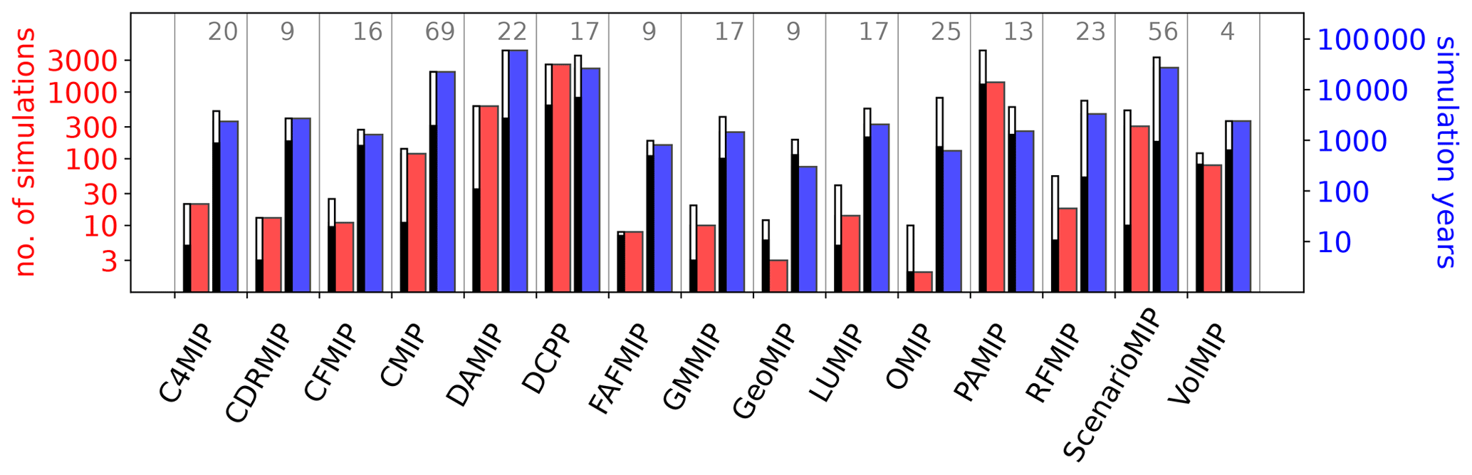
Figure 1 CanESM5.0 number of simulations (red) and total simulation years (blue) contributed to experiments defined by CMIP6-endorsed MIPs. For each MIP, thinner inset bars show the median (black) and maximum (white) number of contributions by all models participating in the MIP, with the number of contributing models indicated at top. Determined by a search of the ESGF archive on 22 October 2022 for monthly-mean atmospheric near-surface temperature (tas), precipitation (pr), ocean surface temperature (tos) and surface salinity (sos).

2 Analysis in support of model development

The focus of model development is to produce new model versions for use in applications (such as CMIP). Here, “model version” is synonymous with model finalization, whereby all properties of a model are decided and held fixed (model resolution, dynamical core, formulation of physical parameterizations, assignment of free parameters, etc.). Such model versions are assigned a version number, or ID, for reference (the naming convention for CanESM versions is described in Sect. 3). A primary goal of model development is to bring about improvement in the model properties and behaviour with each succeeding version. To accomplish this, model development efforts generally focus on systematic errors, or issues, that have been found with the properties and behaviour of recent and predecessor model versions.

Model issues are generally first identified as a simple bias in some quantity relative to observations, but ideally they would ultimately be connected to and understood in terms of the specific representation of physical processes or dynamical mechanisms in the model. While there are potentially many ways to characterize model issues, we have found it useful to broadly categorize them into three types:

• Version-specific issues are unique to a particular model version; by definition they are due to changes made in that version relative to its predecessor.

• Model-systemic issues are shared across multiple versions of a model; such issues have proved relatively insensitive to recent development efforts.

• Community-systemic issues are systematic errors shared by multiple diverse climate models (e.g., across CMIP ESMs) and are typically due to a community-wide issue related to the absence, or manner of treatment, of one or more physical processes.

The utility of categorizing issues in this way is that it provides an indication of where the sources of the biases potentially reside, which could subsequently be investigated by sensitivity tests in the next round of model development. For example, to resolve a version-specific issue, the focus of such tests should be directed toward all changes made since the predecessor version; for a model-systemic issue, focus should shift away from the changes made over the last several model versions toward other model aspects; and for a community-systemic issue, focus should be directed toward properties shared by other climate models.

Ideally, model development would involve an iterative process in which each new candidate version would undergo a comprehensive evaluation exercise to gauge the success of development efforts and to inform the utility of that version for its intended applications. However, given the complex nature of model development and tight deadlines associated with large projects such as CMIP, there is typically insufficient time and resources to iteratively undertake the breadth of experiments and subsequent diagnostic analysis that would be required to derive such insight. Each modelling centre meets this challenge in some undocumented manner in the finalization of production versions of their ESM.

At the CCCma, we have recently focused on this challenge and initiated a new activity, Analysis for Development (A4D), to critically review existing procedures and to develop strategies to evaluate new versions of our Earth system model, CanESM. There are three primary objectives of A4D:

• The first is to make more systematic and increase our efforts to resolve model issues. To this end, a regular A4D meeting (separate from model development meetings) was established, and two lead scientists were appointed to coordinate and oversee its activities. Through such meetings, issues with CanESM are reviewed and their potential sources discussed. A more detailed, deep-dive, scrutiny of some issues is undertaken by starting working groups to independently investigate specific issues through additional analysis and sensitivity tests. As a result of the A4D initiative, we now better engage CCCma's full resources to identify and maintain focus on model issues. While a large portion of a climate laboratory's scientists are engaged in model development, typically a much smaller subset are responsible for bringing the major components together to obtain a new ESM version with acceptable properties and behaviour (e.g., biases relative to observations and responses to external forcings such as climate sensitivity). With the A4D initiative, we have chosen to make the acceptance of new ESM versions a group-wide responsibility. The value of this approach is that it engages all CCCma staff – particularly those with extensive analysis expertise who might not typically engage in model development activities – and it provides a process to engage the expertise of external colleagues in the academic community.

• The second is to better document our efforts to resolve model issues – including both successes and failures. To this end, a new GitLab A4D issue tracker was established on the same GitLab version control system used to manage all of the CanESM code base, which is used to keep track of, permanently document and discuss our efforts to resolve model issues.

• The third is to make more systematic and increase our efforts to identify and monitor model issues. To this end, a new A4D standardized diagnostic package is being developed. Systematic and automated evaluation of climate model versions has been highlighted by the community as an important tool for advancing model development (e.g., Gleckler et al., 2016; Eyring et al., 2016, 2020). All working groups are required to propose metrics that are salient to the issue they are tasked with investigating (even if that issue was eventually resolved). The collection of such CanESM-specific metrics, along with more standard diagnostics, are brought together to form a suite of diagnostics that can be run automatically. The advantages of such an automatic package are that it can be applied to the model at any time during development, provide early detection of new issues, be used to monitor the occurrence and severity of known issues across model versions, and remove the burden from individual scientists to reproduce their analysis on future versions long after their working group responsibilities have ended. The output of this package is organized in standardized diagnostic reports and posted on the public CanESM GitLab page for key model versions (https://gitlab.com/cccma/canesm/-/wikis/home, last access: 3 November 2023).

The rest of the paper documents results from the A4D activity. This includes substantial contributions to the development of a new and improved version of CanESM, CanESM5.1, and a number of deep-dive analyses that provide insight into the origin and possible elimination of systematic model biases in CanESM.

3 Models and experiments

3.1 CanESM5.0

Swart et al. (2019b) described the model characteristics and climatological properties of CanESM5.0, which was also referred to as “CanESM5” in that study, and has the precise version name CanESM5.0.3. The CCCma uses a three-digit naming convention for our models: Major.Minor.Patch. Changes in the patch version represent technical changes which generally do not alter the bit pattern (and are tested not to alter the climate) and are not advertised externally, changes in the minor version number represent the incorporation (or activation) of new physics and technical changes within the existing model components, and changes in the major version number represent wholesale replacement or major changes to the model basic components. Further changes to model configuration, such as adjustment of tunable parameters, can also be represented by the physics variant label, as described further below.¹ Following this naming convention, the CanESM version from Swart et al. (2019b), CanESM5.0.3, is referred to publicly as CanESM5.0 and is distinguished by its minor version number from CanESM5.1, which is the new CanESM version described in Sect. 3.2.

CanESM5.0 represented a major change compared to its predecessor CanESM2 (Arora et al., 2011; von Salzen et al., 2013), CCCma's Earth system model that contributed to most of the experiments of CMIP5. Compared to CanESM2, CanESM5.0 includes completely new models for the ocean, sea ice and marine ecosystems, as well as a new coupler, while the atmosphere, land surface and terrestrial ecosystem models improved incrementally. The resolution of CanESM5.0 is T63 spectral with 49 vertical levels for the atmosphere and nominally 1^∘ with 45 vertical levels for the ocean. This is similar to that of CanESM2 and at the lower end of CMIP6 models, allowing for more simulation years (and larger ensemble sizes) to be achieved than other CMIP6 models with higher resolution.

Two CanESM5.0 model variants, labelled by the physics variant labels p1 and p2, have been released, as described in Swart et al. (2019b). Compared to the p1 variant, the p2 variant featured improved remapping of wind-stress fields passed from the atmosphere to the ocean and the removal of a bug that led to cold spots over Antarctica. It should be noted, though, that for most variables differences between the simulated mean climate and its response to forcing are generally small and physically insignificant. Here we use the p2 version, which will be referred to in this paper as CanESM5.0 or CanESM5.0-p2. For further details on CanESM5.0, we refer the reader to Swart et al. (2019b).

3.2 CanESM5.1

CanESM5.1 is a new version of CanESM for which two model versions labelled p1 and p2 have been released. The distinctions between the p1 and p2 variants are described below (Sect. 3.2.1). It is important to note that the differences between the p1 and p2 variants of CanESM5.1 are completely independent from, and unrelated to, the differences between the p1 and p2 variants of CanESM5.0. Figure 2 summarizes the evolution from CanESM5.0 to CanESM5.1, listing the key model changes for each version and its variants. The following main improvements compared to CanESM5.0 are common to both versions of CanESM5.1:

• The first is a retuning of parameters associated with the hybridization of advective tracers, including dust and moisture. In particular, the dust hybridization parameters were poorly tuned in CanESM5.0, which led to unrealistic spikes in dust burdens. These improvements and impacts on the simulation of stratospheric temperatures and tropospheric dust will be described in Sect. 5.1.

• The second is an improved remapping of atmospheric heat fluxes that are passed to the ocean grid within the coupler, by changing to a second-order conservative scheme (Jones, 1999) that preserves a smooth derivative across grid cells.² This helped to reduce the nonphysical “blocky” pattern in the heat fluxes on the ocean grid (see Fig. A1).

• Very significant technical changes were implemented in the structure of the source code of the Canadian Atmospheric Model (CanAM), the atmospheric general circulation model component of CanESM, with the syntax updated from pre-Fortran 77 to free-form Fortran (F90+) and, more significantly, a major reorganization of array structures within the model to improve efficiency and flexibility. An important objective behind these changes was to facilitate the interfacing of the CanAM physics with different dynamical cores (and specifically GEM; Qaddouri and Lee, 2011), as well as to provide quality-of-life improvements for developers such as making configurable parameters available in input lists rather than hard-coded. The syntax changes provide bit-identical results (i.e., they preserved the bit pattern of the model results). The changes to array structure are not bit-identical but had no statistically discernible impact on the model climate.

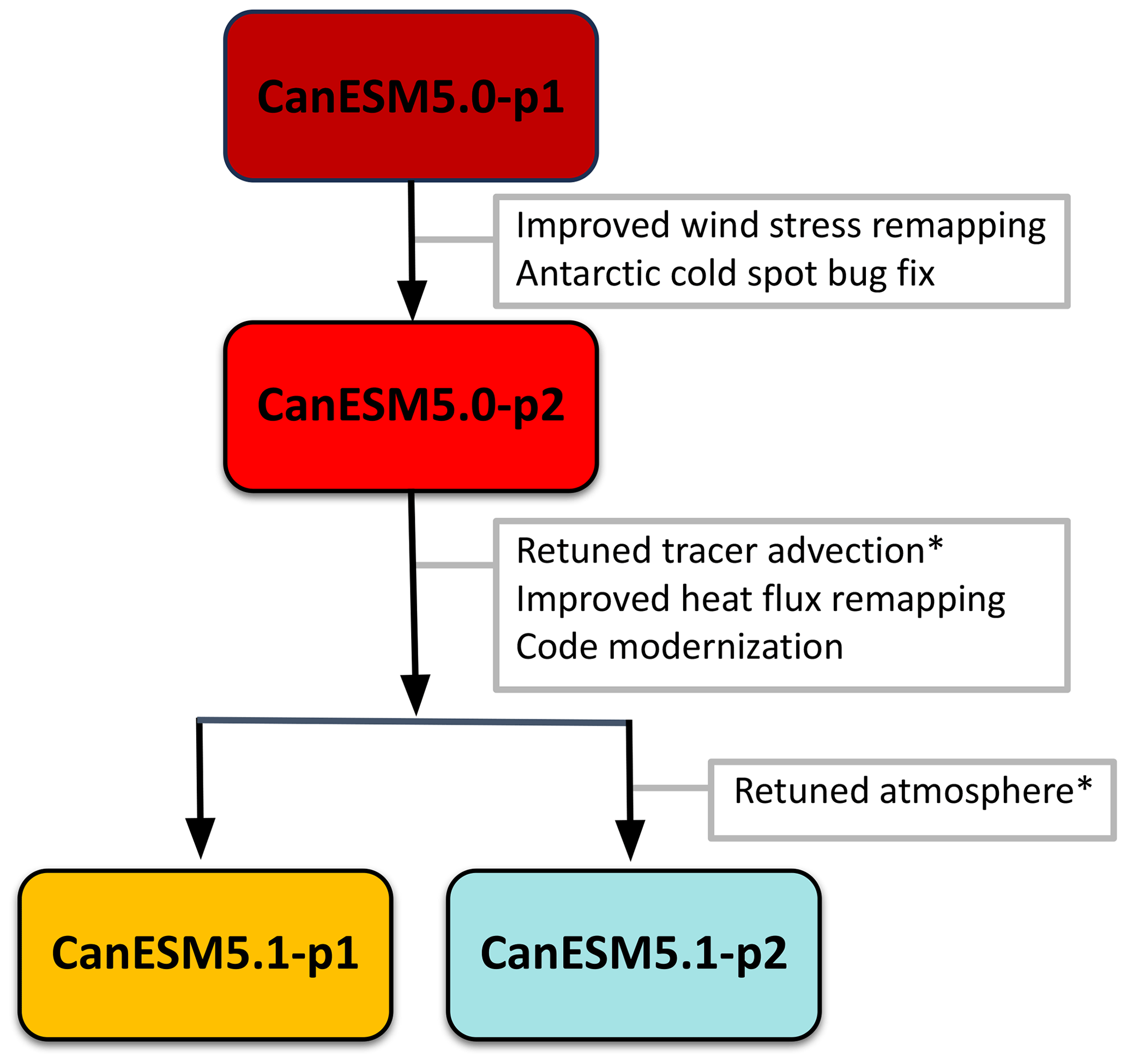
Figure 2 Schematic indicating model development history from CanESM5.0 to CanESM5.1 and their variants (p1 and p2). The text in grey boxes summarizes the model changes implemented in the version(s) to which the arrows point. Model improvements labelled with an asterisk are the result of the A4D activity (see the main text for further details).

3.2.1 The p1 and p2 variants of CanESM5.1

The source code of both p1 and p2 variants of CanESM5.1 is essentially identical, with the two model versions differing only in the tuning of parameterizations in the atmospheric component of the model (as indicated in Fig. 2). As will be shown in Sect. 4, the physical climate of the p1 variant of CanESM5.1 is virtually indistinguishable from both the p1 and p2 variants of CanESM5.0.

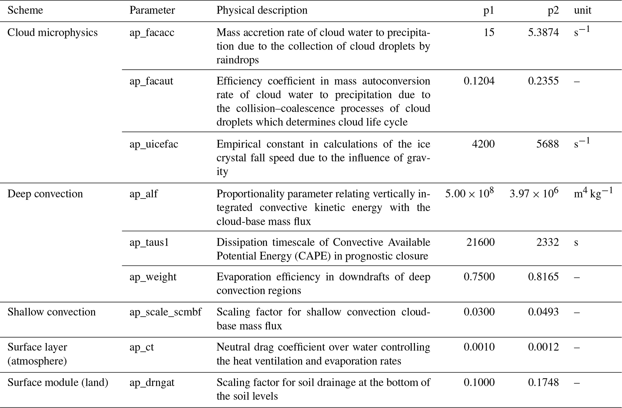
The climate characteristics of the p2 version of CanESM5.1, by contrast, are quite different, as the atmospheric component of CanESM5.1-p2 was retuned to best match historical warming, El Niño–Southern Oscillation (ENSO) amplitude and ENSO seasonality. The goal of this retuning exercise was to investigate the extent to which an alternative parameter tuning could (1) alleviate the high bias in historical warming of our CMIP6 model (CanESM5.0, and equivalently CanESM5.1-p1) and (2) improve the skill of CanESM5.1-p1 seasonal-to-decadal forecasts for which the representation of the ENSO is crucial. This tuning was accomplished by adjusting the nine free parameters summarized in Table 1 within their physically plausible ranges. The impacts of this retuning exercise on ENSO variability and climate sensitivity will be described in Sect. 5.2.

Table 1 Summary of the nine tuned parameters for the p1 and p2 variants of CanESM5.1.

3.3 Experiments

3.3.1 CMIP experiments

Pre-industrial control experiments and large ensembles of experiments with standard CMIP6 historical forcings (i.e., the CMIP6 “historical” experiments) were run and uploaded to the ESGF system, consisting of 40 members for CanESM5.0-p2, 47 members for CanESM5.1-p1 and 25 members for CanESM5.1-p2.³ These runs are used for the analysis in this paper. Note that we use all ensemble members, except when explicitly mentioned. In such cases, fewer ensemble members were needed to obtain robust conclusions. In addition, single member abrupt-4xCO2 and SSP5-8.5 experiments, also available on the ESGF system, are used here to study the response climate change.

Note that the strong similarity in physical climate between three of the CanESM versions that are available on the ESGF system (CanESM5.0-p1 and p2, and CanESM5.1-p1) supports combining these into a single large ensemble for those applications that could benefit from this size of historical ensemble (25 members of CanESM5.0-p1, 40 members of CanESM5.0-p2 and 47 members of CanESM5.1-p1, giving 112 members in total).

3.3.2 Sensitivity experiments

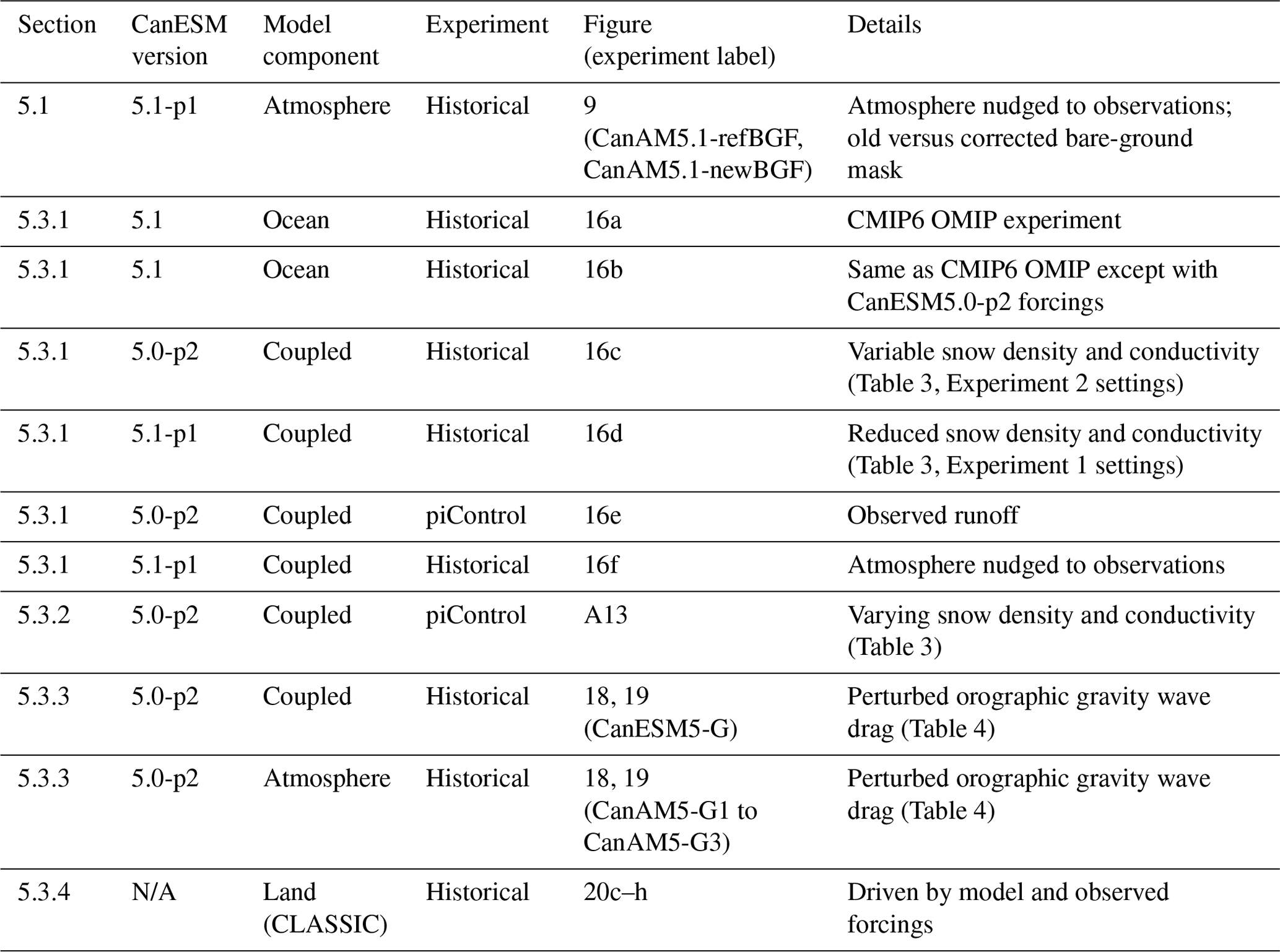
In addition to the standard CMIP-style experiments, the A4D activity has led to a number of bespoke experiments run to gain understanding of the causes of several notable CanESM5.0 and CanESM5.1 biases. Details of these sensitivity experiments are presented in Table 2 and are used in the analysis presented in Sect. 5.1 and 5.3.

Table 2 Details of the sensitivity experiments. Note that for the OMIP experiments, no p version is specified, as for those experiments CanESM5.1-p1 is equivalent to CanESM5.1-p2.

4 Basic comparison between CanESM5.0 and CanESM5.1

4.1 Historical mean climate

In this section, we provide a high-level comparison between the model characteristics of CanESM5.0 and the two variants of CanESM5.1. As documented in Swart et al. (2019b), CanESM5.0 reproduces the large-scale features of the observed climate but suffers from several regional biases. As shown in Fig. 3a and d, these biases include a cold bias over sea-ice-covered regions in winter in both hemispheres (further discussed in Sect. 5.3.2); a cold bias over the Tibetan Plateau (Sect. 5.3.4); warm biases over the eastern boundary current systems, the Amazon, and North America in summer; and a cold bias in the North Atlantic associated with a positive sea-ice bias (Sect. 5.3.1 and Fig. A3). This positive North Atlantic sea-ice bias results in an overestimation of total Arctic sea-ice area in winter (Fig. 4a); a similar North Atlantic bias is found in one other CMIP6 model (CAMS-CSM1-0; Fig. 5c). By contrast, September Arctic sea-ice area only shows a very small (positive) bias, which is among the smallest among CMIP6 models as shown by Fig. 5a. CanESM5.0 shows a year-round overestimation of Arctic sea-ice volume compared to the observation-based product PIOMAS (Fig. 4b). In the Antarctic, CanESM5.0 generally simulates too much sea ice (Fig. 4c), and in austral winter this positive bias is largest among the CMIP6 models considered here (Fig. 5b).

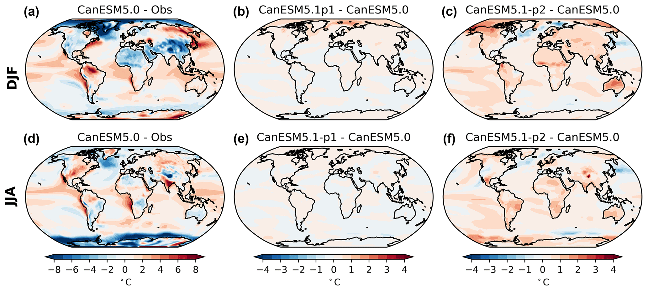
Figure 3 Ensemble-mean surface air temperature bias relative to ERA5 (Hersbach et al., 2020) in CanESM5.0 (a, d) and the ensemble-mean difference between CanESM5.1-p1 and CanESM5.0 (b, e) and between CanESM5.1-p2 and CanESM5.0 (c, f), averaged over 1981–2010 for the December–February (DJF; a–c) and June–August (JJA; d–f) seasons. Note the different contour intervals for (a) and (d) compared to (b), (c), (e) and (f).

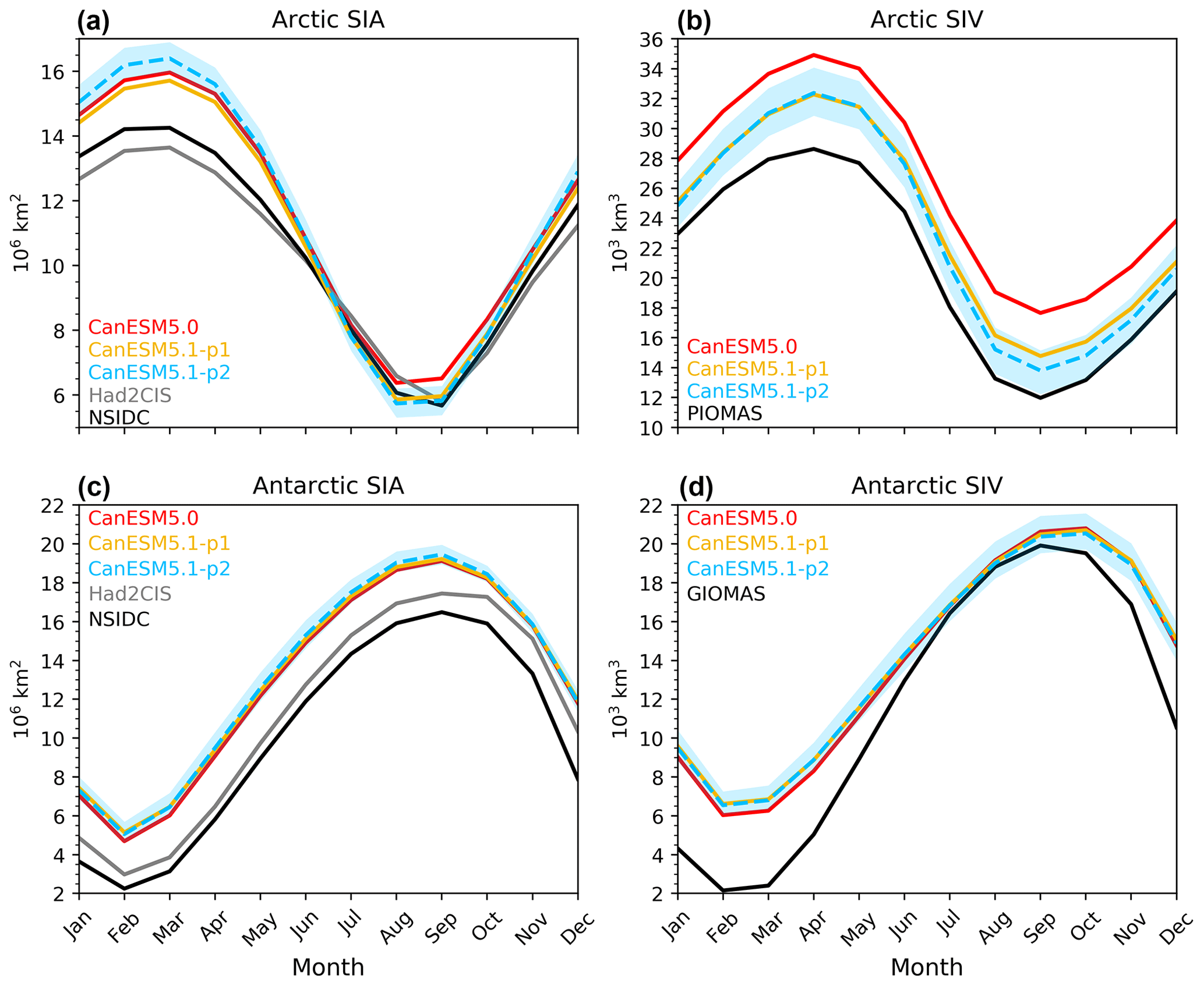
Figure 4 Seasonal cycles of sea-ice area (SIA) (a, c) and sea-ice volume (SIV) (b, d) in the Northern Hemisphere (a, b) and the Southern Hemisphere (c, d), averaged over 1981–2010, for CanESM5.0, CanESM5.1-p1, CanESM5.1-p2, NSIDC (Meier et al., 2021) and Had2CIS (Lin et al., 2020) for sea-ice area, as well as the PIOMAS and GIOMAS reanalyses (Zhang and Rothrock, 2003) for sea-ice volume. The lines represent the ensemble means, and the blue shading represents the ensemble range in CanESM5.1-p2.

Compared to CanESM5.0, CanESM5.1-p1 has a slightly warmer Arctic winter (Fig. 3b). While Arctic sea-ice area is slightly smaller in CanESM5.1-p1 (Fig. 4a), the main cause of these slightly warmer temperatures is likely the thinner sea ice, as the Arctic sea-ice volume is smaller (and closer to PIOMAS) than in CanESM5.0 (Fig. 4b). Apart from these small differences, the climates of CanESM5.0 and CanESM5.1-p1 are virtually indistinguishable, as supported by panels (b) and (e) of Figs. A2–A8.

Differences between the historical climates of CanESM5.1-p2 and CanESM5.0 are larger. The pre-industrial climate in CanESM5.1-p2 is 0.5 ^∘C warmer than that of CanESM5.0 and CanESM5.1-p1, with a global mean surface air temperature of 13.8 ^∘C in CanESM5.1-p2 versus 13.3 ^∘C in CanESM5.1-p1 and CanESM5.0 (not shown). While CanESM5.1-p2 warms less over the historical period (as described below), its global mean surface temperature is still slightly higher than that of CanESM5.0 when averaged over 1981–2010 (Fig. 3c, f). Cloud fraction is generally lower than in CanESM5.0 and CanESM5.1-p1, especially over the ocean (Fig. A2). The warmer surface temperatures are consistent with a warmer troposphere (Fig. A7c, f), a larger tropical wet bias (Fig. A5c, f) and a stronger subtropical jet (Fig. A8c, f). In addition, the strong stratospheric polar vortex bias that was seen in CanESM5.0 is slightly larger in CanESM5.1-p2, which has implications for sudden stratospheric warmings (Sect. 5.3.3). An exception to the warmer temperatures in CanESM5.1-p2 is the North Atlantic, which experiences a slightly larger cold bias (Fig. 3c, f). This is consistent with a slightly larger wintertime high sea-ice bias, both in the North Atlantic (Figs. 5c and A3c) and over the entire Arctic (Fig. 4a). For mean biases in other physical aspects of the historical climate, we refer to the reports published at the CanESM GitLab page (https://gitlab.com/cccma/canesm/-/wikis/home, last access: 3 November 2023).

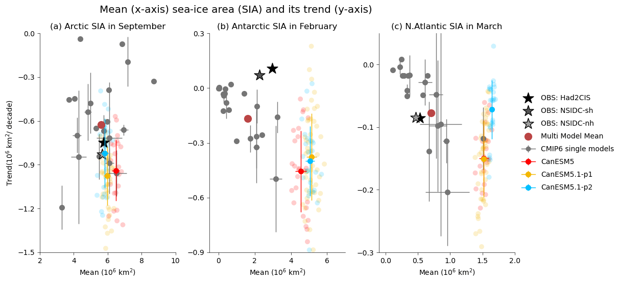
Figure 5 The 1981–2010 climatological mean (horizontal axis) versus historical trends (vertical axis) in September Arctic sea-ice area (SIA) (a), February Antarctic SIA (b) and March North Atlantic SIA (c). Stars indicate observations, grey dots indicate ensemble means of CMIP6 models, small coloured solid dots indicate the ensemble means of CanESM5.0 and CanESM5.1, the large red dot indicates the CMIP6 ensemble mean, horizontal and vertical bars indicate the across-ensemble standard deviations for models with multiple ensemble members, and the faint coloured dots indicate the individual ensemble members of the CanESM5.0 and CanESM5.1 simulations. The figure is an updated version of Fig. 3.20 from IPCC AR6 WGI (Eyring et al., 2021).

4.2 Climate change

As documented by Swart et al. (2019b) and shown in Fig. 6a, CanESM5.0 simulates more historical warming than in observations, while historical September Arctic sea-ice trends are very close to observations (Fig. 5a, vertical axis). This implies that the September sea-ice decline per degree of global warming is underestimated, which is a common model bias (Notz and SIMIP Community, 2020). Historical Antarctic sea-ice trends are negative as in almost all other CMIP6 models (Roach et al., 2020), which appears inconsistent with the positive historical trends in observations (Parkinson, 2019; Fig. 5b). Although, we note that, as a result of internal variability in CanESM5.1-p1, 3 of 47 ensemble members (6 %) simulate a positive Antarctic sea-ice trend in February (for CanESM5.1-p2, it is 1 of 25 members, 4 %), suggesting that CanESM5.1 is consistent with observations.

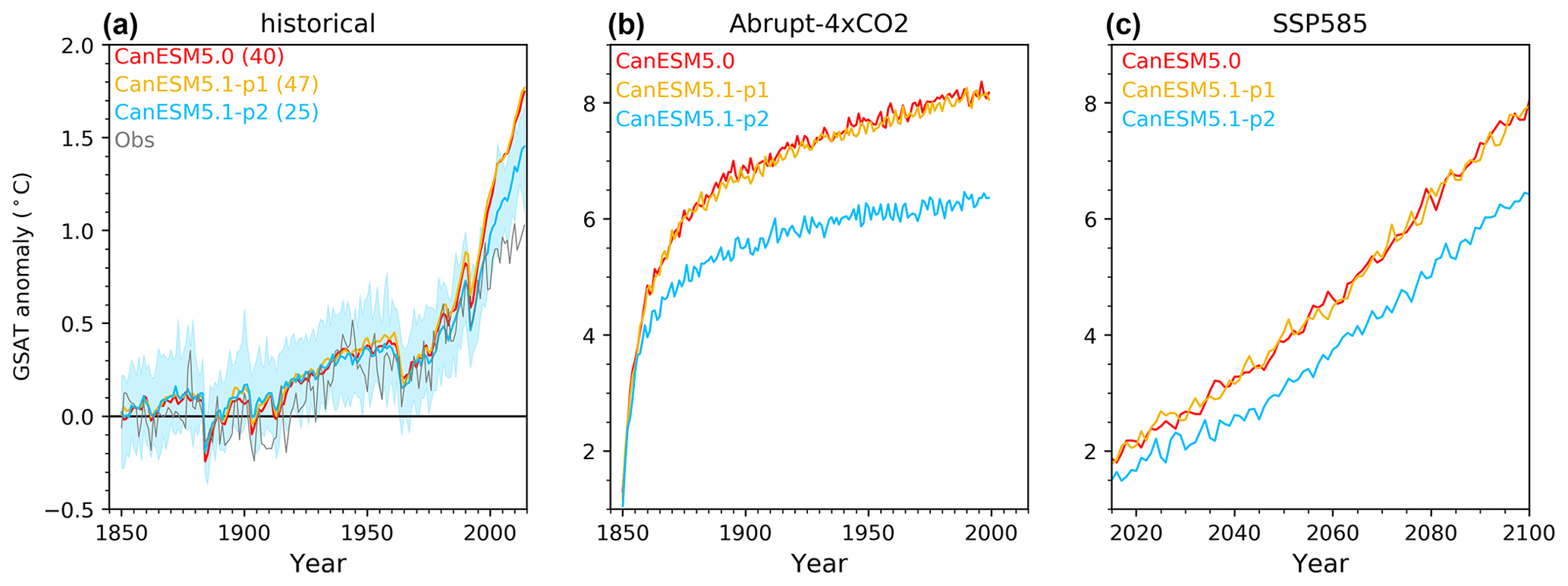
Figure 6 Global mean surface air temperature (GSAT) anomaly relative to the mean in the piControl runs in CanESM5.0-p2, CanESM5.1-p1 and CanESM5.1-p2 for (a) historical, (b) abrupt-4xCO2 and (c) SSP5-8.5 simulations. In panel (a) the coloured lines represent the ensemble mean, the blue shading is the ensemble range in CanESM5.1-p2, the grey line is the observed anomaly relative to the 1850–1900 mean from HadCRUT5 (Morice et al., 2021) and the number in the legend indicates the ensemble size. Only one ensemble member was available for the simulations plotted in panels (b) and (c).

While historical global warming (Fig. 6a) and sea-ice trends (Fig. 5) in CanESM5.1-p1 are virtually identical to those in CanESM5.0, historical warming in CanESM5.1-p2 is about 20 % weaker than in CanESM5.0 (Fig. 6a) as a result of the atmospheric model tuning described in Sect. 3.2.1. The lower warming rate is also seen in the abrupt-4xCO2 simulations (Fig. 6b), used in Sect. 5.2.2 to calculate the equilibrium climate sensitivity, and in future projections such as the projection that follows the SSP5-8.5 scenario (Fig. 6c). We note, though, that while the historical warming in CanESM5.1-p2 is closer to observations, the lower end of the global mean surface air temperature (GSAT) ensemble spread (blue shading in Fig. 6a) still exceeds observations after 2005, implying that historical warming is still biased high. Finally, we point out that historical Arctic and Antarctic sea-ice area trends in CanESM5.1-p2 are similar to those in CanESM5.0 and CanESM5.1-p1 (Fig. 5a, b), with the exception that historical winter trends in North Atlantic sea-ice are somewhat smaller and more consistent with observations (Fig. 5c).

5 Model characteristics and systematic model biases

In this section, we provide more detailed analyses of specific model biases and characteristics in CanESM5.0 and CanESM5.1. We start with the improvements in CanESM5.1 compared to CanESM5.0 that are the result of the improved dust tuning (Sect. 5.1). This is followed by a description of changes in ENSO characteristics and climate sensitivity between the two variants of CanESM5.1 as a result of the retuning of the atmospheric component (Sect. 5.2). Finally, Sect. 5.3 describes the analysis of a number of outstanding biases in CanESM5.0 and CanESM5.1, which in most cases have led to promising paths to resolving these biases in future versions of CanESM.

5.1 Improvements in CanESM5.1 compared to CanESM5.0: dust tuning

Recent analyses have revealed some unrealistic features in CanESM5.0, including the occurrence of spurious stratospheric temperature spikes in certain ensemble members of its historical large ensemble (Santer et al., 2021) and spurious tropospheric dust storms. Subsequent testing and analysis revealed that both of these features were the result of improperly tuned free parameters associated with the “hybridization” of the fine- and coarse-mode mineral dust tracers in CanESM5.0. Hybridization is a transform applied to tracer variables designed to reduce their dynamic range and alleviate artefacts associated with the spectral advection of positive definite tracers (von Salzen et al., 2013). However, the advected tracer mass may not be conserved as a consequence of the hybridization, depending on the values of two free hybridization parameters. Conservation of global tracer mass is ensured in CanESM by correcting the tracer mass following each advection time step (von Salzen et al., 2013), and improper tuning of the hybridization parameters associated with mineral dust resulted in anomalously large mass corrections in some instances. Subsequent retuning of these parameters reduced the magnitude of the mass corrections in CanESM5.1 and eliminated spurious stratospheric warming events and tropospheric dust storms that were present in CanESM5.0, as we document here. As these features were not present in CanESM2 and have been corrected in CanESM5.1, they can be considered version-specific issues.

We first describe the spurious lower-stratospheric warming spikes in CanESM5.0 and their relationship to the mineral dust spikes. Figure 7a shows the monthly time series of global mean lower-stratospheric temperature anomalies in the first ensemble members of CanESM5.0, CanESM5.1-p1 and CanESM5.1-p2. All three model versions show multi-month warming peaks in response to the major volcanoes and long-term cooling in response to increasing carbon dioxide concentrations, but only CanESM5.0 shows ∼1–2-month warming spikes that cannot be explained by external forcings. To more clearly highlight these warming spikes, we subtract the ensemble-mean time series (which averages out internal variability and hence represents the forced response), which leaves the part of the temperature anomalies that is due to internal variability and is hereafter referred to as the unforced variability (Fig. 7b). It appears that the warming spikes coincide with large peaks in the global coarse mineral dust burden (Fig. 7c). This is further quantified in Fig. 7d, which shows the relationship between the dust and temperature spikes in all months of all available ensemble members. It clearly shows a positive correlation between coarse-mode mineral dust burden and unforced lower-stratospheric temperature. It also shows that elimination of coarse mineral dust spikes in CanESM5.1-p1 and CanESM5.1-p2 is associated with the elimination of lower-stratospheric temperature spikes. Lagged scatter plots reveal that there is no correlation between coarse mineral dust spikes and the lower-stratospheric temperature in the prior month (Fig. A9a), which is evidence that the temperature spikes are the result of and not the cause of the dust spikes. They also show that there is a weak impact of coarse mineral dust spikes on lower-stratospheric temperature in the following month (Fig. A9b), and that this impact does not last for longer than a month (Fig. A9c, d). Further analysis revealed that the coarse mineral dust spikes (defined as spikes whose global burden exceeds 12×10⁹ kg) occur once every ∼50 years (mainly in boreal summer) (Fig. A10a), rarely last longer than 2 months (Fig. A10b) and have a maximum impact on zonal mean temperature in the low-latitude lower stratosphere (Fig. A11).

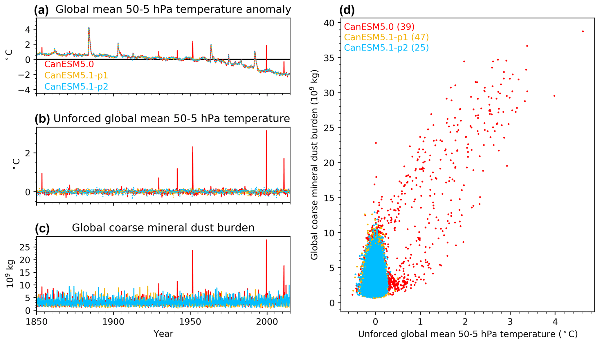
Figure 7 Lower-stratospheric temperature spikes and their relation to coarse mineral dust. The monthly time series of (a) global mean lower-stratospheric temperature anomalies, (b) unforced variability in the global mean lower-stratospheric temperature (details in text), (c) total global coarse mineral dust burden in the first ensemble member of each model version and (d) a scatter plot of the unforced global mean lower-stratospheric temperature versus total global coarse mineral dust burden in all months of all ensemble members.

We next document the impact of the improved hybrid mineral dust tracer tuning in CanESM5.1 on the aerosol optical depth (AOD). A more detailed analysis shows that dust AOD in CanESM5.0 is primarily associated with concentrations of fine-mode tropospheric dust and less so with stratospheric coarse-mode dust (not shown). Differences in seasonality of the fine and coarse dust are plausible, given that they have rather different spatial distributions and are therefore subject to different transport processes, including uplifting and deep convection.

Figure 8 shows total aerosol optical depth from 2007–2014 (Fig. 8a, c) and the mean seasonal cycle over that time period (Fig. 8b, d) in CanESM5.0-p2, CanESM5.1-p1, and CanESM5.1-p2. Also shown are remotely sensed AOD observations from the Moderate Resolution Imaging Spectroradiometer (MODIS, dashed lines; Platnick et al., 2017; King et al., 2013), Multi-angle Imaging SpectroRadiometer (MISR, dash–dot lines; Diner et al., 1998) and the Cloud-Aerosol LIdar with Orthogonal Polarization (CALIOP, solid lines; Winker et al., 2009). These datasets are described in Appendix B.

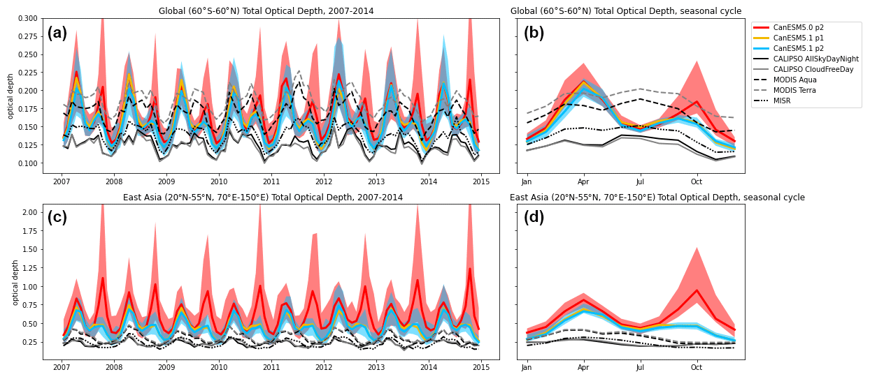
Figure 8 Time series (a, c) and mean seasonal cycles (b, d) of near-global mean (60^∘ S–60^∘ N; a, b) and East Asian (20–55^∘ N, 70–150^∘ E; c, d) total AOD at 550 nm in CanESM5.0-p2 (and CanESM5.1-p1 and CanESM5.1-p2) and in remotely sensed observations (black and grey). For the models, solid lines indicate ensemble medians and shaded envelopes indicate the 5th-to-95th percentile range across ensemble members. The ensemble spread of CanESM5.1-p1 is omitted for visual clarity but is similar to that of CanESM5.1-p2.

Figure 8a and b show near-global-mean AOD (restricted to 60^∘ S–60^∘ N to facilitate comparison with observations), and Fig. 8c and d show AOD over eastern and central Asia. The time period 2007–2014 is chosen because 2007 is the earliest year for which all observational data products are available, and 2014 is the last year of the historical simulation.

In CanESM5.0, events with high AOD were predominantly associated with dust emissions in eastern and central Asia, with AOD that exceeded 10 locally (near the emission source), and produced extended plumes with aerosol optical depth of order 1 that covered most or all of the northern extratropics. In general, CanESM5.0 was characterized by unphysically high variability in AOD across a range of different timescales, even during time periods that did not produce any notable stratospheric dust spikes (Fig. 8), both regionally and globally (see Jones et al., 2021). Furthermore, periods with high AOD preferentially occurred in boreal spring and autumn, producing a double-peaked seasonal cycle (Fig. 8b, d), with an especially large autumn peak in eastern and central Asia (Fig. 8d). A recent assessment of simulated mineral dust in CMIP6 models (Zhao et al., 2022) identified substantial variability in the regional seasonal cycles simulated by different models, and a number of models exhibit similar double-peaked behaviour over northern China, which the authors attributed to excessive surface wind speeds in autumn and winter. However, CanESM5.0 is unique in the magnitude of this second peak. These issues are substantially improved in CanESM5.1. The retuning of the hybridization parameters removes the mechanism by which mineral dust emission spikes were formed, such that they are absent in CanESM5.1. This correction reduces both the AOD variability and time mean and improves the seasonal cycle relative to observations by substantially suppressing the boreal autumn peak (Fig. 8b, d).

Figure 9 demonstrates the improvement in the spatial pattern and spatial variability of mineral dust optical depth from CanESM5.0 to CanESM5.1, as well as in comparison to remotely sensed observations and other CMIP6 models. Observations of dust optical depth are more uncertain than those of total optical depth, and the observations used here are therefore less reliable than those shown in Fig. 8; these limitations are described in Appendix B.

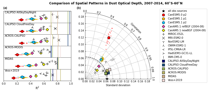
Figure 9 Improvements in the 2007–2014 mean spatial pattern and variability of global dust optical depth from CanESM5.0 to CanESM5.1 compared to observational datasets and select CMIP6 models. (a) Correlation between simulated datasets (points) and six remotely sensed observational datasets. Each row corresponds to a different reference observation, and vertical bars show the correlation between that reference observation and the other five. (b) Taylor diagram comparing simulations and observations to the average dust optical depth field across observational products.

The left panel of Fig. 9 shows the coefficient of determination (R², which indicates how close the distributions fall to a 1:1 relationship), between the spatial patterns of 2007–2014 averaged dust optical depth fields in various model simulations and observational datasets, following Fig. 13h of Zhao et al. (2022). The CMIP6 models included here were selected on the basis of data availability. Rows correspond to different reference observations. Vertical bars give the R² of the other observations against each reference observation, and they can be considered a benchmark of what performance is reasonable to expect from the models. The right panel of Fig. 9 shows a Taylor diagram (Taylor, 2001) of dust optical depths, using as reference the average of the six observational datasets. Note that the “correlation” axis in the Taylor diagram refers to the spatial Pearson correlation coefficient of the patterns, which quantifies how tight the scatter between two quantities is but does not compare the magnitudes of their values. Given the data limitations described in Appendix B, precise position on this diagram should be considered with scepticism, but relative groupings are robust. The left- and right-hand panels of Fig. 9 together demonstrate that while development from CanESM5.0 to CanESM5.1 brought dramatic improvement in the spatial distribution of dust variability (further illustrated in Fig. A12), it brought only modest improvement in the mean spatial pattern. The spatial correlation of both CanESM5.0 and CanESM5.1 with observations remains lower than for other CMIP6 models.

One outstanding issue for dust simulation in CanESM is the estimation of the bare-ground fraction, which is used to determine potential mineral dust sources in the model. An interpolation error has been identified in the bare-ground mask used in CanESM5.0 and CanESM5.1 which led to errors in the input emissions. While this error will be corrected in future versions of CanESM, we here quantify the impact of this error on already existing simulations. This is done by comparing two atmosphere-only simulations (with and without bare-ground fraction correction), in which the atmosphere is nudged to reanalysis so that the observed meteorological conditions, which have a large impact on dust, are well reproduced. We use atmosphere-only simulations with sea surface temperatures (SSTs) and sea ice following observations to exclude the possible impact of SST and sea-ice biases on our results. Comparison of these simulations (denoted by, respectively, the yellow and pink plus sign in Fig. 9) suggests that the correction improves the dust simulation, with the Pearson correlation coefficient increasing from 0.73 with the interpolation error to 0.80 without the error (Fig. 9b). Although the spatial pattern appears improved in this test simulation, the variability is substantially reduced such that the RMSE is approximately unchanged. In addition, the hybridization tuning parameters used in this simulation were not updated to reflect the corrected bare-ground fraction. Thus, while these results are suggestive, they are also preliminary, and further analysis is required to determine whether corrections to the bare-ground fraction are sufficient to make the spatial pattern of dust in CanESM as realistic as that of most other CMIP6 models, as suggested by Fig. 9a.

5.2 Differences between CanESM5.1-p1 and CanESM5.1-p2

The p2 variant of CanESM5.1 was obtained by systematically retuning the atmospheric component in an attempt to reduce biases in ENSO characteristics and historical warming (Sect. 3.2). This section provides a detailed description of the ENSO characteristics and climate sensitivity in various CanESM versions, with a focus on the changes that are the result of the atmospheric tuning in the p2 variant of CanESM5.1 compared to the p1 variant.

5.2.1 ENSO

The ENSO phenomenon, driven by atmosphere–ocean interactions in the near-equatorial Pacific Ocean, is the strongest and most wide-reaching pattern of interannual climate variability. A long-standing objective has therefore been for coupled climate and Earth system models to simulate ENSO realistically in order to better understand and predict ENSO, its global impacts and likely changes in a warming climate.

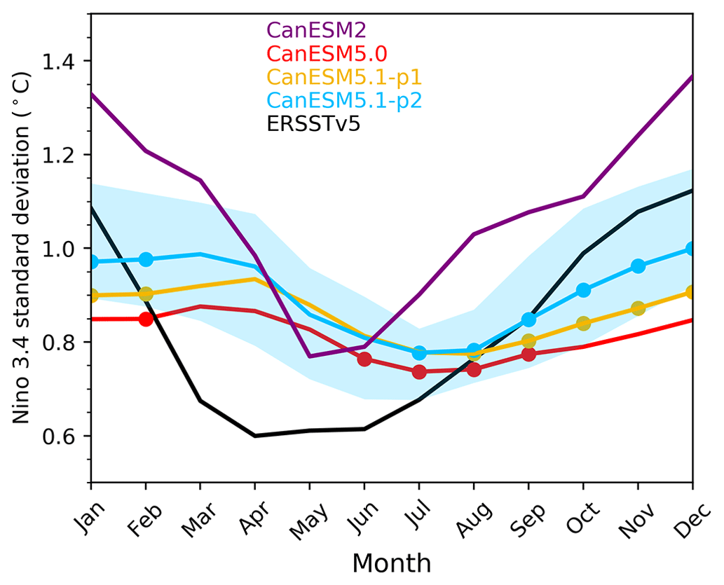
Figure 10 Standard deviations of interannual variability of the Niño 3.4 index (the average SST anomaly in the region bounded by 5^∘ S to 5^∘ N and 170 to 120^∘ W) for each calendar month in 1950–2014. For CanESM5.1-p2, the shading represents the range over 10 ensemble members. Dots indicate months for which the 10 ensemble ranges bracket the observations from ERSSTv5 (Huang et al., 2017).

Many metrics have been devised to describe various aspects of modelled ENSO variability and associated physical processes (e.g., Planton et al., 2021). One common community-systemic bias is that equatorial Pacific SST anomalies associated with warm (El Niño) and cool (La Niña) episodes often extend significantly farther westward than is observed (Jiang et al., 2021). This is the case for CanESM5.0 (Swart et al., 2019b) and the updated versions considered here, as well as for earlier CCCma model versions (Merryfield et al., 2013), making it a model-systemic issue as well. However, there are biases in other aspects of ENSO variability that are version-specific to CanESM5.0 and CanESM5.1, as they differ from its immediate major-version predecessors, CanESM2 and CanCM4.⁴ Of particular note is that the seasonal cycle of ENSO SST variability is relatively accurate in CanESM2 and CanCM4, with strong seasonal differences peaking in December as observed (Guilyardi et al., 2012; Merryfield et al., 2013) and overall ENSO amplitude slightly overestimated, as shown for CanESM2 in Fig. 10. By comparison, Fig. 10 also shows that ENSO in CanESM5.0 is too weak and displays little seasonal variation with a minimum in boreal summer instead of spring and no distinct winter peak, as also reported in Swart et al. (2019b), Planton et al. (2021) and Eyring et al. (2021). This likely bears on why experimental seasonal predictions from CanESM5.0 (not shown) are considerably less skilful at predicting future ENSO evolution out to 12 months than CanCM4, which has relatively high ENSO prediction skill relative to other operational seasonal prediction models (e.g., Ham et al., 2019). On the other hand, Fig. 11 shows that the distribution of ENSO variability across timescales is more realistic in CanESM5.0, with the CanESM2 spectral peak occurring at shorter periods than for the observed spectrum, whereas for CanESM5.0 the distribution of spectral power is closer to that of the observed time series.

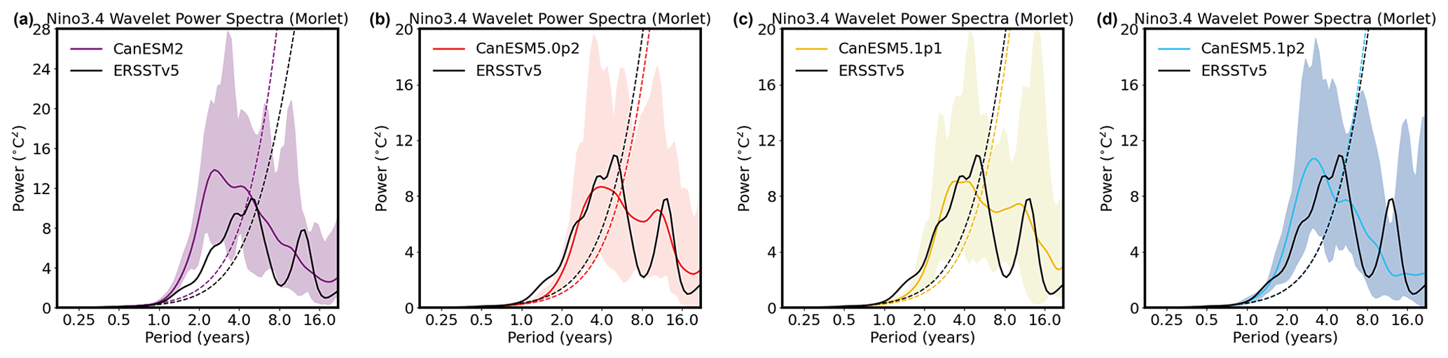
Figure 11 Power spectra of detrended monthly Niño 3.4 anomalies during 1950–2014 for (a–d): CanESM2, CanESM5.0, CanESM5.1-p1 and CanESM5.1-p2. Black curves represent spectra of the observed time series from ERSSTv5, coloured curves represent the mean of the spectra from 20 ensemble members, and shading represents the range of those spectra. Spectra are obtained from wavelet transforms based on the Morlet wavelet (Torrence and Compo, 1998), and dashed curves represent the 95 % confidence level for a red-noise background spectrum. Note the different vertical scale for CanESM2.

While the p1 variant of CanESM5.1 has slightly higher ENSO variability than CanESM5.0, its seasonal cycle peaks in March as in CanESM5.0, which is inconsistent with the December peak in observations (Fig. 10). The impact of the atmospheric retuning on ENSO variability can be seen by comparing the p1 and p2 variants of CanESM5.1. Figures 10 and 11 show that in CanESM5.1-p2 the ENSO amplitude is indeed higher than in CanESM5.1-p1, and that the seasonal cycle is somewhat improved with a December peak, although overall the seasonal variation remains too weak.

Some insights into why ENSO seasonality is too weak in CanESM5.0 and CanESM5.1 can be gained from several recent studies comparing ENSO and climatological SST seasonality in CMIP5 and CMIP6 models. The climatological seasonal cycle (annual mean subtracted) of equatorial Pacific SST from observations and the three model versions are compared in Fig. 12. All are concentrated in the eastern part of the domain where the thermocline is relatively shallow. Notably, the observed seasonal cycle primarily consists of the first annual harmonic despite the semi-annual cycle of insolation, whereas all CanESM5 versions display a distinct semi-annual component in the east (Fig. 12c–e). Song et al. (2020) evaluated the simulated eastern equatorial Pacific SST seasonal cycle in CMIP5 and CMIP6 models. They found that the correlation between the simulated and observed seasonal cycle in the region 110–85^∘ W where the seasonal cycle is strongest is only 0.55 for CanESM5.0, the lowest among 17 CMIP6 models considered, whereas for CanESM2 it is much higher (0.87). This suggests a connection between how realistically the equatorial Pacific SST seasonal cycle and ENSO seasonality are modelled, in accordance with studies indicating that they are linked (e.g., Neelin et al., 2000).

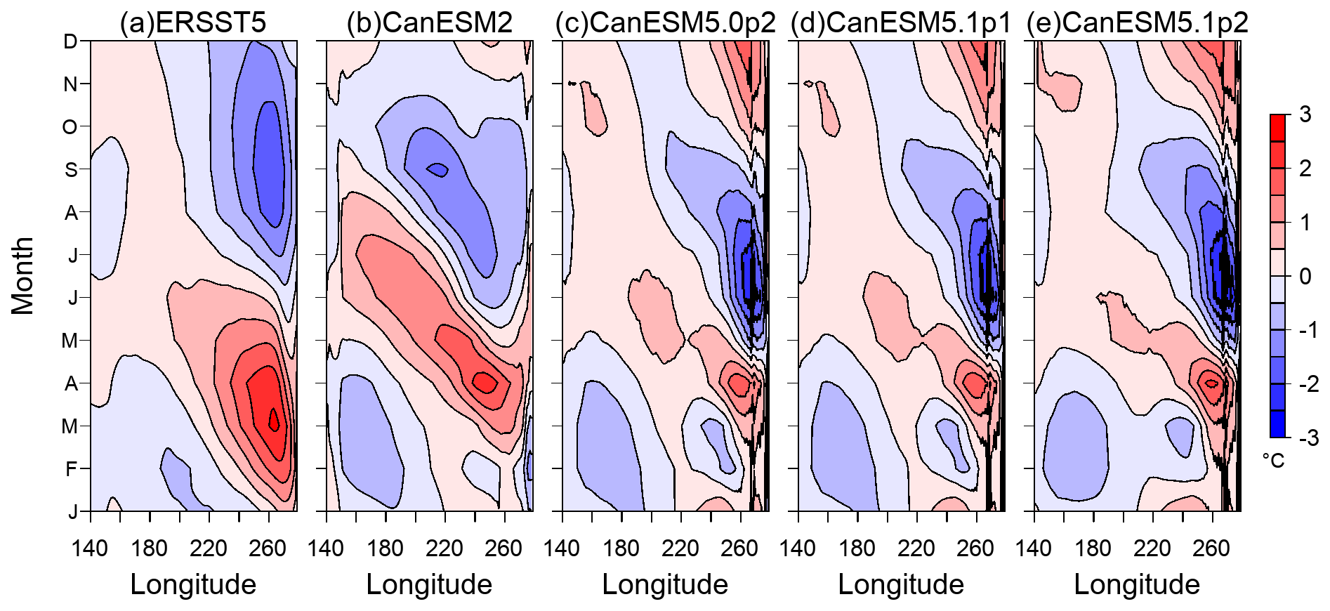
Figure 12 Mean seasonal cycle (i.e., the monthly minus annual means) of equatorial Pacific SST during 1950–2014 for (a) ERSSTv5, (b) CanESM2, (c) CanESM5.0p-2, (d) CanESM5.1-p1 and (e) CanESM5.1-p2. Each model version is represented by the mean of the first 10 ensemble members.

A pair of additional studies have examined ENSO seasonality in terms of its phase-locking to the mean seasonal cycle across numerous CMIP5 and CMIP6 models. Liu et al. (2021) showed that the month of peak ENSO variability and the distribution over different calendar months in which ENSO events peak in CanESM2 are among the most realistic of all models considered, whereas CanESM5.0 is among the most unrealistic; they argued that the fidelity of the simulated SST seasonal cycle may be a major factor responsible for such differences. Liao et al. (2021) applied different metrics but ranked the performances of CanESM2 and CanESM5.0 in simulating ENSO seasonality, similarly to Liu et al. (2021), and furthermore associated ENSO seasonality biases with biases in representing the seasonal zonal equatorial SST gradient. They found the temporal correlation of observed and modelled seasonality of a metric describing the large-scale zonal differences⁵ to be among the lowest in CanESM5.0 of all models considered. Such a calculation based on the CanESM versions considered here and the OISSTv2 dataset (Reynolds et al., 2007) for 1982–2021 yields the same value of 0.49 for CanESM5.1-p1 and for CanESM5.0. This correlation is modestly improved to 0.56 in CanESM5.1-p2, in accordance with the similarly modest improvement in ENSO seasonality in Fig. 10.

The hypothesis that ENSO seasonality biases across CanESM5.0 and CanESM5.1 versions are tied to biases in the simulated mean seasonal cycle, as strongly suggested by the above results, raises the question of how those climatological biases can be reduced. CanESM5.0 and CanESM5.1 employ different atmosphere and ocean model components than CanESM2, making it difficult to assess whether one or the other is primarily responsible for the degradation of climatological and ENSO seasonality between these model versions. However, comparisons presented in Merryfield et al. (2013) between CanCM4, whose ENSO-related metrics are nearly the same as for CanESM2 according to Planton et al. (2021), and the earlier model version CanCM3 provide some insights. In particular, the mean seasonal cycle of equatorial Pacific SST is very similar between these two coupled models, which employ the same CanOM4 ocean model but different atmospheric model versions.⁶ This strongly suggests that the change from CanOM4 in CanESM2 to CanNEMO (Madec and the NEMO team, 2012) in CanESM5.0 and CanESM5.1, which involves many differences in the grid configuration, numerics and physical parameterizations, may be the main underlying reason for the equatorial Pacific seasonal cycle changes between CanESM2 and CanESM5.0 and CanESM5.1. The relative insensitivity to atmospheric model differences in the CanESM5 versions described here aligns with this view. Which specific attributes of CanNEMO should be examined in this context is not obvious, because the mean seasonal cycle of equatorial Pacific SST is governed by a complex interplay of both oceanic and atmospheric processes (Wang and McPhaden, 1999), indicating that considerable model experimentation will likely be required.

5.2.2 Climate sensitivity

A second metric that was used to tune the p2 version of CanESM5.1 was historical warming, which was unrealistically high in CanESM5.0 (Swart et al., 2019b) and is about 20 % weaker than in CanESM5.0 and the p1 version of CanESM5.1 (Sect. 4.2). Here we quantify the associated change in climate sensitivity, and compare that with the climate sensitivity in other versions of CanESM. The metric that we use is the effective climate sensitivity (EffCS), which is based on the regression method of Gregory et al. (2004). In addition, we decompose top-of-atmosphere (TOA) radiative feedbacks using radiative kernels. Non-cloud radiative feedbacks were calculated using radiative kernels from the Community Atmosphere Model (CAM3; Shell et al., 2008). Climate responses for temperature, water vapour, surface albedo and cloud radiative effects (CREs; long wave (LW) and short wave (SW)) were calculated as the mean over years 125–150 of an abrupt-4xCO2 simulation relative to a 100-year mean from a pre-industrial control simulation. Cloud feedbacks were calculated using the adjusted cloud radiative effect (Soden et al., 2008), where the CRE is adjusted according to differences between clear- and total-sky non-cloud feedbacks (Chung and Soden, 2015). The adjusted CRE method assumes that clouds dampen the instantaneous radiative forcing (IRF, the radiative forcing associated with a particular forcing agent assuming that all other variables are held fixed) by 16 % (Soden et al., 2008). Hence, the total-sky IRF is calculated by multiplying the clear-sky IRF with a globally uniform proportionality constant of $\mathrm{1}/\mathrm{1.16}$. Then, taking the difference between the two yields the portion of the IRF from clouds.

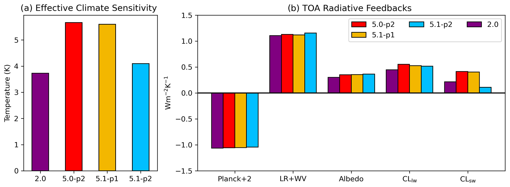
Figure 13 (a) Effective climate sensitivity (EffCS) and (b) global, annual mean TOA radiative feedbacks (in W m⁻² K⁻¹). From left to right, feedbacks are listed as Planck +2 (for display purposes), lapse rate + water vapour, surface albedo, long-wave cloud and short-wave cloud.

As described in Swart et al. (2019b) and Virgin et al. (2021) and shown in Fig. 13a, CanESM5.0 has an EffCS of 5.65 K, making it the CMIP6 model with the highest climate sensitivity (Zelinka et al., 2020). Since its EffCS is 54 % larger than that of CanESM2, the issue is considered version-specific (it cannot be termed a bias since the true value of EffCS is unknown). Virgin et al. (2021) showed that while no single feedback fully explains this increase, the increase in the short-wave cloud feedback explains over half (1.08 K), as shown in Fig. 13b. They further showed that this increase in short-wave cloud feedback comes primarily from a decreased boundary layer cloud fraction over subtropical eastern ocean basins and that this is also reflected in the warming rate asymmetry in the Pacific ocean, where the eastern versus western equatorial Pacific warming difference was larger in CanESM5.0 than in CanESM2 – also known as the pattern effect (Dong et al., 2020).

As expected based on the almost identical tuning settings of their atmospheric components, the EffCS and associated feedbacks in CanESM5.1-p1 are almost identical to those in CanESM5.0. By contrast, Fig. 13a shows that the atmospheric tuning in CanESM5.1-p2 reduced the EffCS to 4.09 K, a reduction of 28 %. TOA feedback decomposition reveals that this is due to a decrease in the SW cloud feedback, which is substantially weaker relative to CanESM5.1-p1/CanESM5.0 (Fig. 13b).

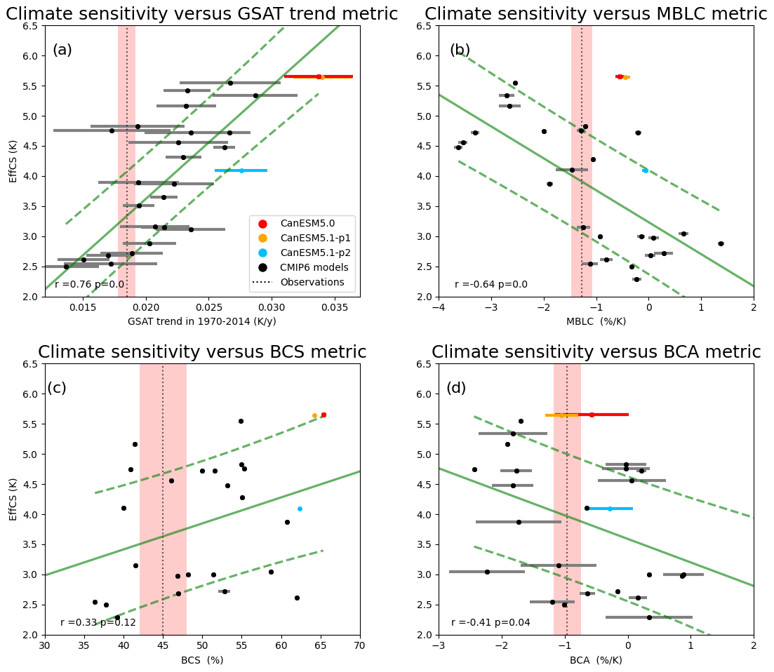
Figure 14 Scatter plots showing relationships between EffCS and observable metrics that have previously been shown to correlate with climate sensitivity across multi-model ensembles, in CanESM5.0 and CanESM5.1 and CMIP6 models: (a) the 1970–2014 global mean near-surface air temperature trend; (b) the sensitivity of marine boundary layer cloud (MBLC) fraction to SST changes in subsiding regions over oceans between 20 and 40^∘ in both hemispheres (Zhai et al., 2015); (c) Brient cloud shallowness (BCS), defined as the ratio of cloud fraction below 900 hPa to that below 800 hPa over weakly subsiding tropical ocean regions (Brient et al., 2016); and (d) Brient cloud albedo (BCA), defined as the sensitivity of the deseasonalized short-wave cloud albedo to SST changes over the tropical oceans (Brient and Schneider, 2016). Error bars show ±1 standard deviations across realizations (i.e., initial condition ensembles) for each model. The dashed vertical lines show the mean observed value, and the red shading shows its ±1 standard deviation, defined as follows: for GSAT in (a), from the 200-member HadCRUT5 ensemble; for MBLC in (b), the estimate of internal variability as described in Zhai et al. (2015); for BCS in (c), 1 seasonal standard deviation as described by Brient et al. (2016); for BCA in (d), an estimate of internal variability obtained by bootstrapping random samples of varying time series length (Brient and Schneider, 2016). The correlation coefficients (between constraints and EffCS over all CMIP6 models) and corresponding p values are reported in the lower left corner of each panel. The dashed green lines in each panel show the 66 % confidence interval of the linear regression model. In all four cases, a two-sample t-means test indicated that metrics were significantly different between CanESM5.1-p1 and CanESM5.1-p2, at the 0.01 level.

Previous studies have shown that SW cloud feedback and climate sensitivity across CMIP5 and CMIP6 models correlate well with the shallowness of low cloud in weakly subsiding tropical regions (Brient et al., 2016; Liang et al., 2022). It appears that CanESM5.0 has the strongest high bias in Brient cloud shallowness (BCS; Brient et al., 2016) among all the CMIP6 models (Fig. 14c), contributing to its high climate sensitivity. The BCS of CanESM5.1-p1 is slightly lower than that of CanESM5.0, which may be due to the fact that the retuning of the hybridization parameters from CanESM5.0 to CanESM5.1 described in Sect. 3.2 also affects moisture and hence clouds. The atmospheric retuning in CanESM5.1-p2 resulted in an even lower BCS and hence a slightly smaller high bias relative to observations. Given the multi-model relationship between BCS and EffCS evident from Fig. 14c and other studies (Brient et al., 2016; Liang et al., 2022), it is likely that this slight BCS reduction contributes modestly to CanESM5.1-p2's lower climate sensitivity. These results suggest that tuning future model versions to further reduce BCS would make such model versions agree better with observations in terms of BCS itself as well as in terms of historical warming (Fig. 14a). This result is further strengthened by the findings of Vogel et al. (2022b), who find that many models overestimate short-wave cloud feedbacks compared to observations. A similar analysis of the sensitivity of cloud fraction and cloud albedo to SST variations over the tropics, which also correlate with SW cloud feedback (Fig. 14b and d), shows only relatively small changes between CanESM5.1-p1 and CanESM5.1-p2, which explain only a small fraction of the decreased climate sensitivity. Moreover the changes in these metrics make CanESM5.1-p2 less consistent with observations than CanESM5.1-p1. These results suggest that tuning future model versions to reduce the amount by which tropical cloud fraction decreases with SST warming (i.e., to further increase MBLC and BCA metrics) should be avoided.

5.3 Other CanESM5.0 and CanESM5.1 biases and possible avenues to tackle them

5.3.1 North Atlantic biases

The North Atlantic is characterized by prominent biases in CanESM5.0, which occur throughout the year, but are largest toward the end of winter. By March, there is excessive sea ice covering the Labrador Sea and Denmark Strait (Fig. 15b), a cold bias in sea surface temperature (SST; Fig. 15d)) and a fresh bias in sea surface salinity (SSS; Fig. 15f).⁷ A corresponding bias exists in surface air temperatures, which are too cold over the North Atlantic in both winter and summer (Fig. 3). CanESM2 also exhibited some of these biases, but they were in general far less pronounced (Fig. 15, left column). Hence the large North Atlantic biases in CanESM5.0 are a version-specific issue. North Atlantic Deep Water formation, one of the primary drivers of the Atlantic Meridional Overturning Circulation (AMOC), relies on deep convection within the Labrador and Greenland–Iceland–Nordic (GIN) seas. The presence of unrealistically high sea-ice coverage over the Labrador Sea in CanESM5.0 inhibits the sea surface buoyancy loss that destabilizes the surface layer and leads to deep mixing (Kostov et al., 2019). Within CanESM5.0, the AMOC is fairly weak (∼13 Sv (sverdrup) in the climatological average), and deep convection is confined exclusively to the shelves of the GIN seas.

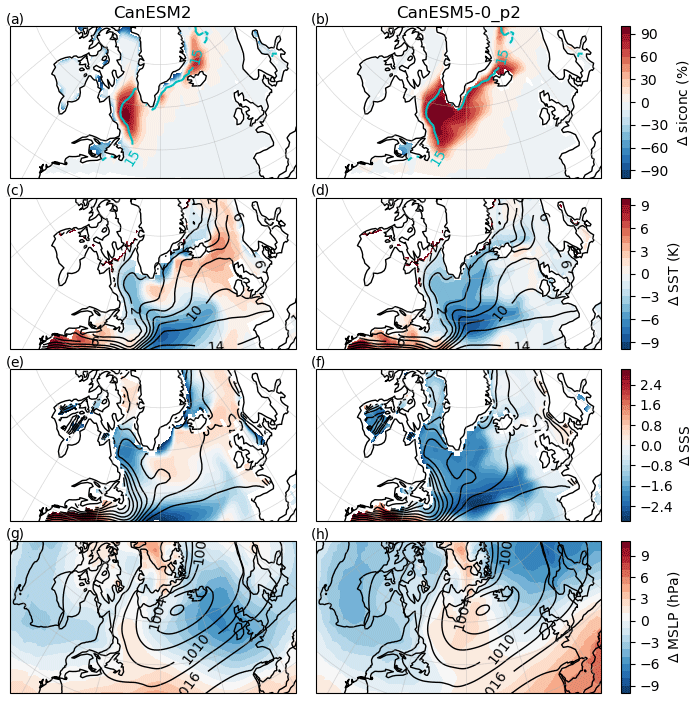
Figure 15 North Atlantic biases during March in CanESM2 and CanESM5.0-p2, relative to observations (named in round brackets). In sea-ice concentration (NSIDC) (a, b), sea surface temperature (Hadley Centre Sea Ice and Sea Surface Temperature, HadISST; Rayner et al., 2003) (c, d), sea surface salinity (WOA13) (e, f) and sea level pressure (ERA5) (g, h). In all cases, biases are shown as colours and were computed from historical experiments in CanESM, over the period 1981–2010 for the month of March. Black contours show the March climatologies from the observations.

The biases in sea ice, SST and SSS in CanESM5.0 are clearly interconnected, but determining cause and effect in the coupled CanESM system is far from trivial. During the development of CanESM5.0, two sensitivity tests with the coupled model were performed that provided some insights. The first test involved running piControl runs with alternative strengths of ocean vertical diffusivity. These showed very similar biases, suggesting that the biases are not the result of improperly tuned vertical diffusivity. The second test involved restarting the ocean model from rest after the atmosphere had spun up. In this test run, the sea ice, SST and SSS biases developed within a few decades, which pointed to atmospheric biases as a potential source of the coupled biases.

To learn more about the nature of the coupled biases, we here present additional sensitivity tests, starting with more constrained, ocean-only experiments. In the CMIP6 Ocean Model Intercomparison Project (OMIP) experiment, the same ocean model configuration as used in CanESM5.1 is driven by reanalysis-based atmospheric forcing through bulk formulae, with runoff from observations and relaxation toward observed SSS (Griffies et al., 2016). Under observed atmospheric forcing, no such biases in sea ice, SST or SSS exist (Fig. 16a). This indicates that the ocean and sea-ice components of CanESM5 are able to simulate a more realistic state given realistic surface forcing. Next, we repeat the standard OMIP experiment, but instead of reanalysis forcing, we provide forcing (including SSS restoring) from a CanESM5.0 historical simulation. Under CanESM5.0 forcing, the ocean-only model reproduces the biases seen in the coupled model (Fig. 16b). While it would be tempting to attribute the ocean and sea-ice biases to CanESM5.0 forcings, it is important to realize that the CanESM5.0 forcings themselves have an imprint of the ocean surface biases in CanESM5.0. Therefore, we cannot exclude the possibility that the ocean surface biases are due to deficiencies in the ocean model. In conclusion, while these ocean-only experiments are instructive, they lack coupled feedbacks and do not provide definitive evidence about the cause of the biases or their solutions.

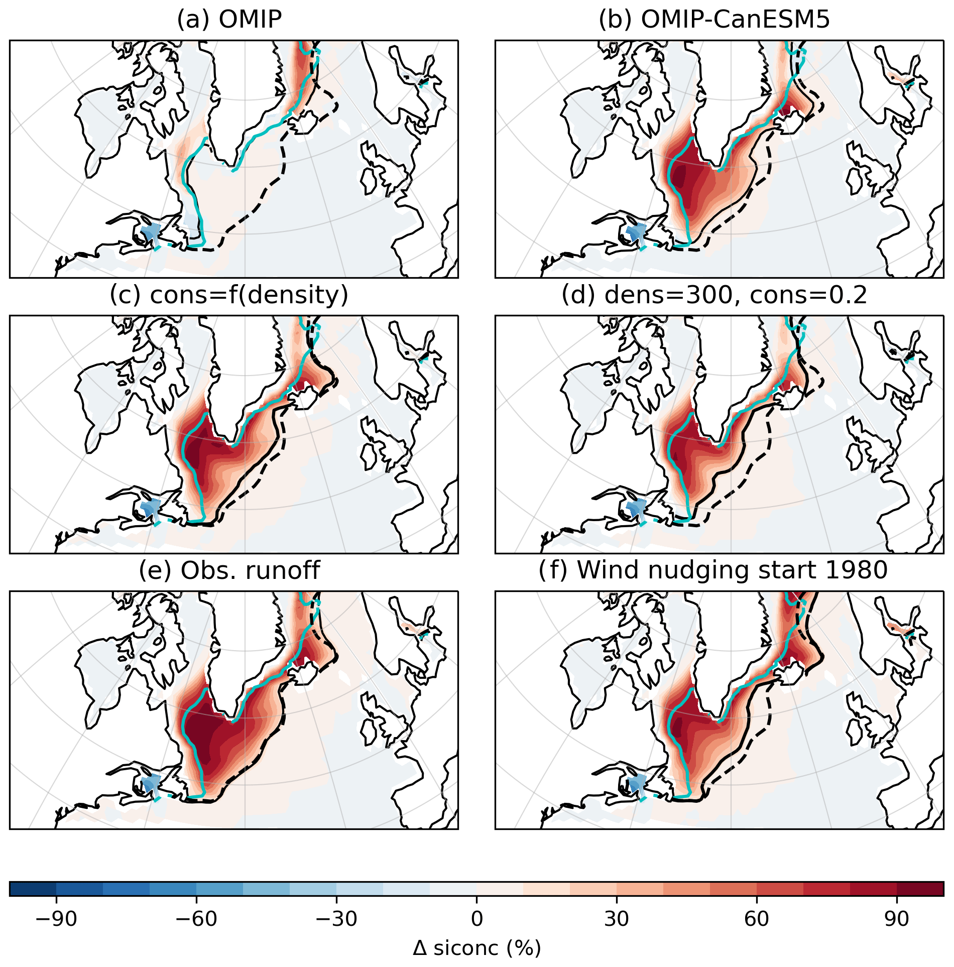
Figure 16 North Atlantic sea-ice concentration bias during March, relative to NSIDC observations in various experiments: (a) the CMIP6 OMIP experiment, forced by reanalysis; (b) an OMIP-like experiment, but forced by CanESM5 historical forcing; (c) coupled historical experiment using variable snow density and conductivity (experiment 2 settings from Table 3); (d) coupled historical experiment using lower values of fixed snow density and conductivity (10 % and 35 % lower, respectively; experiment 1 settings from Table 3); (e) coupled pre-industrial experiment using observed runoff; (f) coupled historical experiment, with nudging of atmospheric vorticity and divergence to ERA5, starting in 1980. Black solid contours give the 15 % concentration contour in the experiment, the dashed black contour is the 15 % contour from the CanESM5 default historical run, and the cyan contour is the 15 % contour from the NSIDC observations. See Appendix C for further discussion of panels (c)–(f).

In Appendix C we explore three hypotheses regarding the origin of the biases in the coupled modelling system, but this investigation has not led to the identification of a definitive cause or solution to the CanESM5 North Atlantic bias. As CanESM moves toward more automated parameter tuning, inline bias correction, a new dynamical core, and new ocean and atmospheric grids resolutions, we hope to arrive at versions with smaller circulation biases. Similarly, new approaches to sea-ice thermodynamics and coupling are being considered. Finally, while the ocean-only model in the configuration forced by observations does not show these issues, it is not certain that the ocean configuration does not contribute to the problem in the coupled model. Recent tests suggest that increasing horizontal ocean diffusivity can also help to reduce the bias by increasing the heat and salt flux into the Labrador Sea. Such ocean physics tuning will be another element considered in future investigation of this issue.

5.3.2 Winter cold bias above sea ice

CanESM5.0 exhibits large cold biases in surface air temperature (SAT) over the region covered by sea ice during the winter season, as described in Swart et al. (2019b) and shown in Fig. 17c and d. This bias also persists in CanESM5.1 (Fig. 3). In contrast, there are not large biases in SST over these regions (see Fig. 15 of Swart et al., 2019b). In CanESM5.0 and CanESM5.1, the surface temperature of sea-ice/snow is computed in CanAM, while the calculation in the sea-ice model, LIM2, is not used prognostically (Swart et al., 2019b). This suggests that the surface temperature computation in CanAM is the source of the issue. This reasoning is supported by the fact that the previous coupled model version, CanESM2, which contained the same CanAM ground temperature computation but completely different sea-ice properties (and a different sea-ice model), also exhibited a similar cold bias over the winter sea-ice-covered area (Fig. 17a, b). In fact, as shown in Fig. 7 of Merryfield et al. (2013), a similar bias existed in CanCM3, two atmospheric model major versions before CanESM5.0 and CanESM5.1 (note they also show the bias for CanCM4, which is a physical-only version of CanESM2). Atmospheric Model Intercomparison Project (AMIP) runs (with specified SST and ice cover) show the same winter-hemisphere cold SAT bias over sea ice, demonstrating that this issue arises in CanAM, as opposed to in the ocean or sea-ice models (Fig. 17e, f). Given its persistence across model versions and experiment types, this cold bias above sea ice is model-systemic. While the bias has been identified in surface air temperature, which is a diagnostic rather than a prognostic model field, a very similar bias exists if the comparison with observations is done based on ground temperature (not shown).

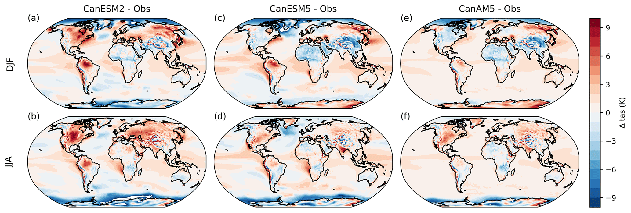
Figure 17 Surface air temperature bias over 1981–2010, relative to ERA5, in CanESM2 (a, b), CanESM5.0-p2 (c, d) and CanAM5.0 (e, f), for the DJF (a, c, e) and JJA (b, d, f) seasons. Note that CanAM5 is an AMIP simulation with no interactive ocean or ice components.

The ground temperature over sea-ice/snow in CanAM evolves according to

$$\begin{array}{}\text{(1)}& \begin{array}{rl}{\mathrm{gt}}_{\left(t\right)}& ={\mathrm{gt}}_{(t-\mathrm{1})}\\ & +(\mathrm{fsg}+\mathrm{flg}-\mathrm{hsens}-\mathrm{hlat}+\mathrm{hsea})\times \mathrm{delt}/\mathrm{cice},\end{array}\end{array}$$

where t is the time step count, gt is the ground temperature (K), fsg is the net absorbed solar flux, flg is the net long-wave flux, hsens is the sensible heat flux, hlat is the latent heat flux, and hsea is the conductive heat flux through ice/snow from the ocean (all fluxes in W m⁻²); delt is the time step duration (s), and cice is the heat capacity of the upper 10 cm of the solid surface (J m⁻² K⁻¹).

Given the winter (and high-latitude) manifestation of this problem, short-wave radiation contributions are unlikely as they occur during polar night, and we have focused on other parts of the surface energy balance. The conduction of heat through sea ice and snow that features prominently in the winter energy balance (i.e., the hsea term in Eq. 1) has been investigated. A series of pre-industrial control experiments were conducted, systematically altering the ice and snow conductivities used in CanAM (Table 3).

Table 3 Pre-industrial control experiments with altered sea-ice thermodynamics in CanAM. In experiment 2, snow density is a function of snow thickness, and snow conductivity is a function of snow density (this scheme was used in CanESM2; McFarlane et al., 1992). In other experiments, snow density and ice/snow conductivities are fixed constants. Experiments 1 and 2 were used as initial conditions (restarts) for historical experiments with the same parameter modifications.

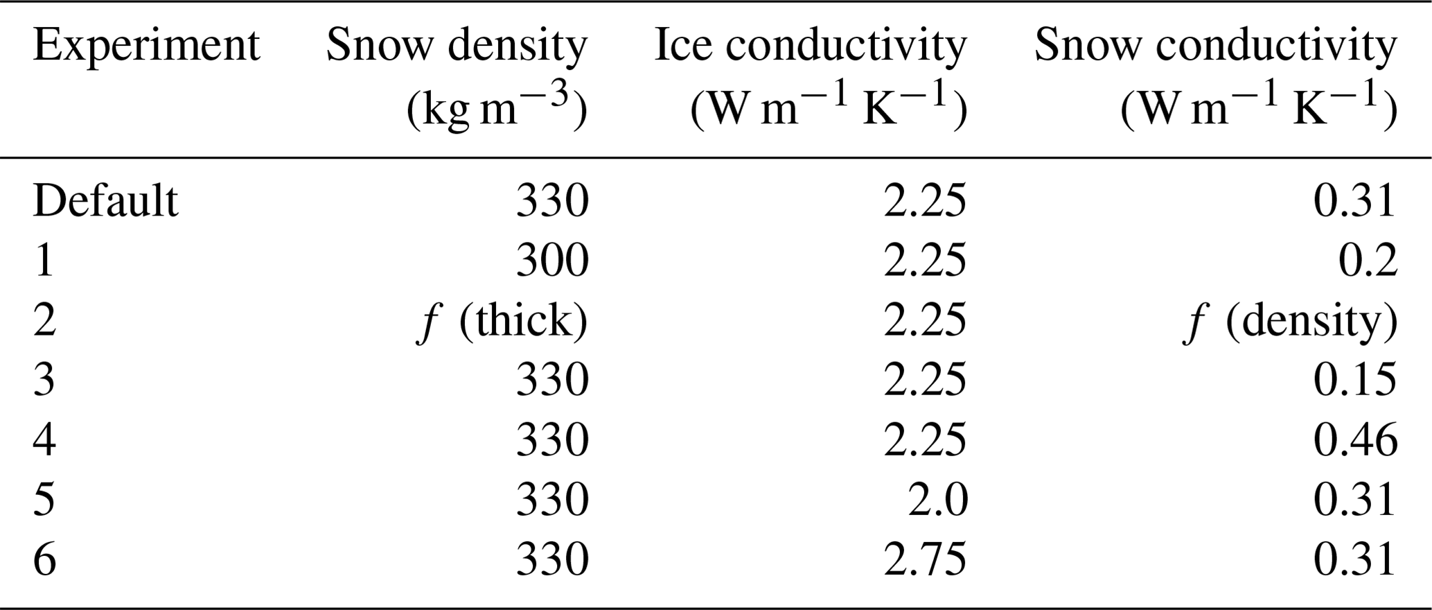
Of these experiments, the largest effect is seen when decreasing the snow conductivity, which leads to some warming of SATs around the edges of Arctic sea ice in DJF (Fig. A13). However, the tested thermodynamic changes only have a small impact relative to the large size of the existing cold bias, and none of them address the systematic and widespread nature of the cold bias (i.e., over all sea ice in the winter hemisphere). Possible alternative explanations for the cold bias above sea ice are issues in the non-solar radiative or turbulent fluxes. Future work will focus on examining these alternative hypotheses.

5.3.3 Stratospheric circulation

In this section, we investigate two atmospheric circulation biases in the stratosphere that have been shown to be important for the simulation of boreal winter surface climate variability and climate change. The first metric of interest is the number of sudden stratospheric warmings (SSWs). SSWs are rapid breakdowns of the westerly flow (or polar vortex) in the polar winter stratosphere, which tend to be followed by a persistent anomalous tropospheric circulation pattern and associated surface temperature and precipitation patterns that can last up to 2 months (e.g., Baldwin et al., 2021). It has been shown that SSWs are a main source of subseasonal to seasonal predictability for surface climate (e.g., Sigmond et al., 2013). Hence, a realistic simulation of SSWs is important for maximizing the skill of seasonal forecasts, particularly in boreal winter and early spring.

Previous multi-model studies have shown that there is a large spread in the simulated frequency of SSWs between different climate models. So called “low-top” models, often defined as those models whose model lid is lower than 0.1 hPa as in Domeisen et al. (2020), tend to underestimate stratospheric variability (Charlton-Perez et al., 2013) and, consequently, the number of SSWs, while “high-top” models tend to simulate a more realistic SSW frequency. The results of Kim et al. (2017) indicate that CanESM2 (a low-top model according to previously mentioned criterion) is a noticeable exception showing an overestimation of the SSW frequency. By contrast, Ayarzagüena et al. (2020) indicates that CanESM5.0 underestimates the SSW frequency. However, it should be noted that the results of both Kim et al. (2017) and Ayarzagüena et al. (2020) are based only on the first ensemble member, and that due to the large internal variability of the coupled stratosphere–troposphere system there can be a large spread between individual ensemble members (Polvani et al., 2017). We first investigate the robustness of the Kim et al. (2017) and Ayarzagüena et al. (2020) results by calculating the SSW frequency in large ensembles of CanESM2 and CanESM5.0 simulations. Figure 18 shows that, averaged over a 50-member initial condition ensemble, CanESM2 simulates about 10 SSWs per decade, confirming the Kim et al. (2017) conclusion (based on the first ensemble member, plotted by the black dot) that CanESM2 overestimates the SSW frequency. Figure 18 also shows that, averaged over a 25-member ensemble, CanESM5.0 simulates too few SSWs, confirming the results of Ayarzagüena et al. (2020), which was based on the first ensemble member. However it should be noted that there is a large spread between ensemble members, and that if Ayarzagüena et al. (2020) had picked a different ensemble member with a SSW frequency at the upper end of the range, they would not have identified CanESM5.0 as one of the models with too few SSWs. Figure 18 also shows that the SSW frequency in CanESM5.1-p1 is very similar to that in CanESM5.0, while that in CanESM5.1-p2 is slightly less. This is consistent with the stronger polar vortex shown in Fig. A8c. Having established the robustness of these differences in SSW frequency between CanESM2 and the latest major CanESM version, underestimated SSW frequency in CanESM5.0 and CanESM5.1 can be considered a version-specific issue.

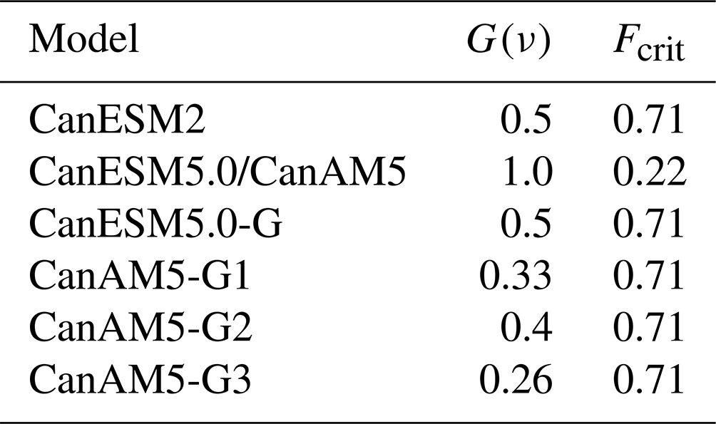
It is striking how different the simulated SSW frequency is in CanESM5.0 compared to CanESM2, given that the model lid height of both models is the same at 1 hPa. One notable difference in the atmospheric component between CanESM2 and CanESM5.0 is in the tuning of the free parameters in the orographic gravity wave drag (OGWD) scheme. The OGWD scheme used in both models is that of Scinocca and McFarlane (2000), which features two internal parameters that were changed between CanESM2 and CanESM5.0: (1) G(ν), a multiplicative factor that scales the amount of gravity wave momentum flux produced by the interaction of the circulation with the topography, and (2) Fr_crit, the inverse critical Froude number, which sets the maximum non-dimensional amplitude that a parameterized wave may attain at launch, before low-level blocking onsets, and aloft before wave breaking begins and the wave begins to transfer its momentum to the background flow. Adjustments to these parameters were made to correct for the weak bias in the polar vortex simulated by CanESM2 (see Table 4). The impact of these OGWD parameter-value changes on the frequency of SSWs is quantified by an ensemble of five historical simulations with CanESM5.0 in which the values of G(ν) and Fr_crit were reset back to those used in CanESM2, hereafter referred to as the CanESM5-G simulations. Figure 18 shows that in these simulations the SSW frequency is very similar to that in CanESM2. This implies that the difference in simulated SSW frequency between CanESM2 and CanESM5.0 can be attributed to the change in OGWD tuning settings.

Having established the strong sensitivity of the SSW frequency to OGWD parameter values, we next perform a series of sensitivity tests in which the values of G(ν) and Fr_crit are adjusted to determine if the low SSW frequency bias in CanESM5.0 could be eliminated. These tests were performed using multiple five-member ensembles of atmosphere-only runs. These runs were branched off from the standard CanAM5 historical runs in 1950. Tuning is performed in atmosphere-only rather than fully coupled mode to speed up the process. This choice is motivated by the observation that the frequency of SSWs is very similar in CanAM5 compared to CanESM5.0, as shown by Fig. 18. Our first combination of OGWD tuning settings are those that have been found to perform best for a previous high top version of our model. The model version with these modified settings is labelled “CanAM5-G1”. A second and third set of tuning runs is performed with slightly higher (CanAM5-G2) and slightly lower (CanAM5-G3) values of G(ν) (details are in Table 4). Figure 18 shows that the settings in CanAM5-G1 yield an overestimation of the number of SSWs. Increasing the OGWD in CanAM5-G2 leads to increased deposition of orographic gravity waves, decreasing the strength of the polar vortex and increasing the number of SSWs, further away from the observed frequency. The decreased OGWD in CanAM5-G3 compared to CanAM5-G1, by contrast, leads to decreased deposition of orographic gravity waves, increasing the strength of the polar vortex and decreasing the number of SSWs and eliminating the high SSW frequency bias in CanAM5-G1. In summary, by varying tuning parameters in the OGWD scheme, we have determined a combination of parameter settings that has eliminated the SSW frequency bias in CanESM5.0. While this combination of parameters has not been implemented in CanESM5.1, it is being considered for future CanESM versions as a way to eliminate SSW biases and maximize the skill that SSWs provide in seasonal forecasts.

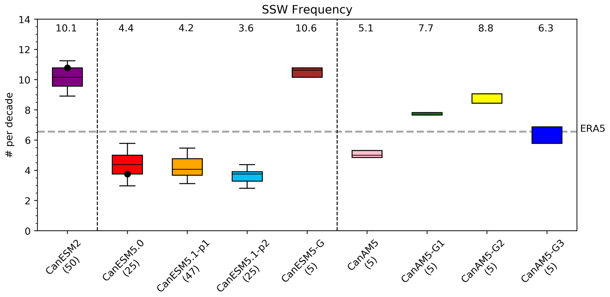
Figure 18 The 1950–2014 frequency of SSWs in various CanESM versions (details in text, with the number in parenthesis after the model name indicating the number of ensemble members) and in the ERA5 reanalysis. The boxes extend from the lower to upper quartile of the ensembles. The black lines represent the medians, the whiskers represent the 5 %–95 % confidence range determined by bootstrapping and the numbers on top of the ensemble-mean represent values. The black dots for CanESM2 and CanESM5.0 indicate the first ensemble members, which were used in Kim et al. (2017) and Ayarzagüena et al. (2020), respectively.

Table 4 Settings of the scaling factor, G(ν), and inverse Froude number, Fr_crit, in the orographic gravity wave parameterization for various CanESM versions.

A second aspect of the stratospheric circulation that is of interest to the surface climate is the strength of the zonal-mean zonal winds in the region between the subtropical jet and the polar vortex (here defined as the wind at averaged over 40–60^∘ N and 100–50 hPa, hereafter referred to as the “neck region winds”). Sigmond and Scinocca (2010) showed that the response of the Northern Annular Mode (NAM) to increasing greenhouse gases (which has large impacts on patterns of regional climate change) is sensitive to biases in the strength of the neck region winds. In particular they found that overly weak neck region winds result in a barrier to equatorward propagation of large-scale atmospheric waves. Climate models consistently show that increasing greenhouse gases result in increased vertical wave fluxes, and Sigmond and Scinocca (2010) showed that in a model version with overly weak neck region winds these increased wave fluxes tend to be deposited at high latitudes, leading to a reduction of the westerly winds and hence a negative NAM response. The opposite was true for a model version with relatively strong neck region winds, which resulted in a positive NAM response to increasing greenhouse gases. This suggests that for credible projections of future regional climate it is important for the neck region winds to be consistent with observations.

The strength of the neck regions winds in various CanESM versions is shown in Fig. 19. It shows that while CanESM2's neck region winds are close to those observed, CanESM5.0's neck region winds are too strong. In response to increasing greenhouse gases Simpson et al. (2018) reported that the polar vortex response in CanESM2 is close to zero, while Karpechko et al. (2022) showed that CanESM5.0 has one of the largest positive polar vortex response among the CMIP6 models. Hence, these findings are consistent with the positive correlation between neck region winds and the NAM response to increasing greenhouse gases as identified by Sigmond and Scinocca (2010). While the neck region winds are similar in CanESM5.1-p1 compared to CanESM5.0, they are even stronger in CanESM5.1-p2. It appears that the change in OGWD settings between CanESM2 and CanESM5.0 can explain about 50 % of the difference in neck region winds, as the neck region wind strength in CanESM5.0-G is between that of CanESM2 and CanESM5.0 (Fig. 19). The neck region winds in CanAM5 are slightly weaker than CanESM5.0, which implies that tuning efforts that target neck region winds should ideally be done in the fully coupled model. Finally, the CanAM5 tuning runs show that while the OGWD combination of CanAM5-G3 led to the most realistic SSW frequency, the bias in the neck region winds is the largest of the three considered OGWD setting combinations. This highlights intrinsic difficulties often encountered in tuning efforts: the improvement of one aspect of the circulation can often lead to the deterioration of another, and focussing on only one aspect of the climate may lead to “overtuning”. This can indicate the absence, or misrepresentation, of a relevant process in the model. For the OGWD scheme in CanAM, a new orographic lift component is being added following the work of Lott (1999) and Gastineau et al. (2020) to better represent stationary planetary waves in CanAM. It is anticipated that improvement of the planetary waves in CanAM will better allow for a simultaneous reduction of biases in both the basic state (including neck region winds) and SSW biases in future versions of CanESM.

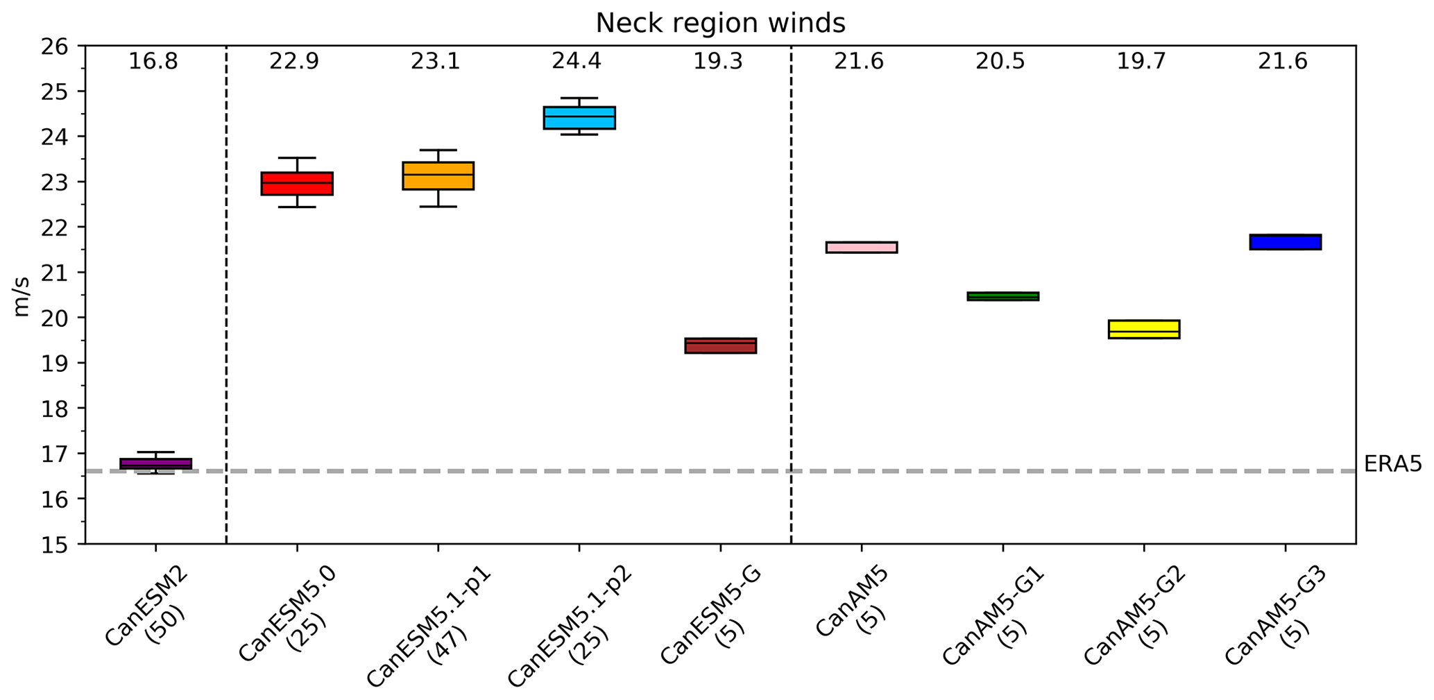
Figure 19 The 1950–2014 and December to February mean neck region winds in various versions of the Canadian Earth System Model (details in the main text, with the number in parenthesis after the model name indicating the number of ensemble members). The boxes extend from the lower to upper quartile of the ensembles. The black lines represent the medians, and the whiskers represent the 5 %–95 % confidence range determined by bootstrapping and the numbers on top of the ensemble-mean values.

5.3.4 Land surface temperatures and albedo

Both CanESM5.0 and CanESM5.1 suffer from a cold bias over the Himalayan region that extends into eastern China, most prominently in December–February (Fig. 3). As a similar bias has persisted over more than one major model version (see Fig. 17a), it is considered a model-systemic issue. This bias is likely caused by two factors. First, a positive precipitation bias in the region leads to more snow and therefore also a positive land surface albedo bias in the region. Second, the current snow fraction parameterization in the land component of CanESM5.0 and CanESM5.1 does not take into account the effect of topography. Compared to regions with flat terrain, the same amount of snow should cover less area in mountainous regions because snow is not able to accumulate on steep terrain (Swenson and Lawrence, 2012). Since this effect is not yet parameterized in CanESM, snow covers a larger fraction than it realistically should in mountainous regions with steep terrain.

Figure 20a shows the bias in simulated annual-mean surface albedo in a CanESM5.0 historical simulation compared to the observation-based product CERES (Kato et al., 2013) for the period 2000–2013 for which the CERES data are available over the southeastern Asian region. The surface albedo bias is largest over the Himalayan region. Figure 20b shows the bias in mean annual snow water equivalent from a historical CanESM5.0 simulation compared to the ECCC observation-based data (Mudryk, 2020), also for the period 2000–2013, and shows the large bias over the Tibetan Plateau. This large amount of snow builds up over time as the model is spun up for conditions corresponding to the pre-industrial state and does not disappear over the historical period. The grid cells in dark blue in Fig. 20b over the Tibetan Plateau region that exceed the 12 cm colour bar scale build up snow amounts varying from 70 to 310 cm in snow water equivalent units.

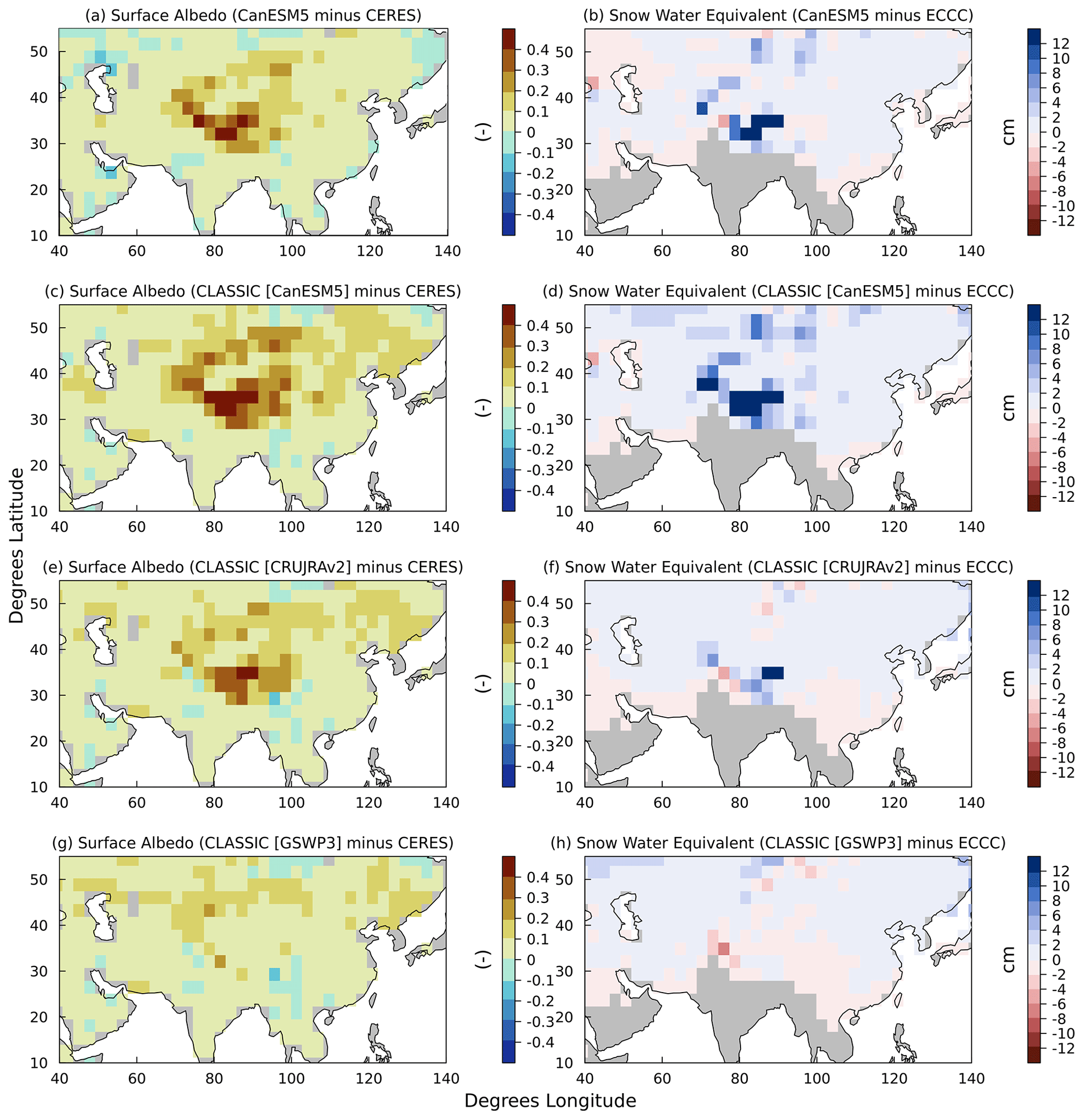
Figure 20 Annual-mean bias in simulated surface albedo for short-wave radiation (left column) and snow water equivalent (right column) compared to the CERES and ECCC observation-based products, respectively, over the southeastern Asian region for the 2000–2013 period. Panels (a) and (b) show the biases for CanESM5.0. Positive values indicate higher model values compared to the observation-based data. The remaining rows show the biases when the CLASSIC land model is driven offline by meteorological data from CanESM5.0 (panels c and d) and from the observation-based datasets CRU-JRA (panels e and f) and GSWP3 (panels g and h). Note that the largest positive biases in snow water equivalent exceed the colour scale shown (see the main text for details).

The land component in CanESM5.0 and CanESM5.1 is represented by the Canadian Land Surface Scheme (CLASS; Verseghy et al., 1993) and the Canadian Terrestrial Ecosystem Model (CTEM; Arora and Boer, 2005). CLASS and CTEM simulate physical and biogeochemical processes, respectively, in the family of CanESM models. CLASS and CTEM will be succeeded in a subsequent CanESM version by the Canadian Land Surface Scheme including Biogeochemical Cycles (CLASSIC), which couples these two models in a unified framework (Melton et al., 2020). CLASSIC includes a very similar version of physical processes, including snow-related physical processes, based on CLASS as in CanESM5.0 and CanESM5.1.

Offline simulations of CLASSIC are routinely performed with various observation-based meteorological datasets to evaluate the model's performance for primary water, energy and CO₂ fluxes in an uncoupled mode where land–atmosphere feedbacks are absent. These simulations have also contributed to the Global Carbon Project (Friedlingstein et al., 2022) since 2016. In these offline simulations, CLASSIC is driven with meteorological data from three different sources: CanESM5.0, the Climate Research Unit Japanese Reanalysis (CRU-JRA) and the Global Soil Wetness Project 3 (GSWP3). The CRU-JRA (v2.1.5) meteorological dataset, which is the Japanese reanalysis (JRA) with monthly values adjusted to the CRU data, provides 6-hourly values of seven meteorological variables that are required to drive a land model such as CLASSIC. These data are provided as part of the Trends in the land carbon cycle (TRENDY) protocol for land models that contribute to the Global Carbon Project (Friedlingstein et al., 2022). Three-hourly meteorological data from CanESM5.0 for the same seven variables are also saved to force CLASSIC offline. Finally, the GSWP3 forcing data are based on a dynamical downscaling of the 20th century reanalysis (Compo et al., 2011) using a global spectral model run at about 50 km resolution and also available at the 6-hourly temporal resolution.

Figure 20c–h show the bias in these offline simulations in simulated annual-mean land surface albedo and snow water equivalent, averaged over the period 2000–2013, compared to CERES and ECCC data, respectively. Positive biases in snow albedo and snow water equivalent over the Himalayan region are simulated when CLASSIC is driven with CanESM5.0 and CRU-JRA meteorology (Fig. 20c–f). The bias is much smaller for snow albedo and of the opposite sign (with a small magnitude) for snow water equivalent when CLASSIC is driven offline with the GSWP3 meteorology. Although other meteorological variables also play some role, the difference in CRU-JRA and GSWP3 runs is largely driven by higher precipitation in CRU-JRA dataset compared to the GSWP3 meteorological dataset over the Himalayan region (Fig. 21i, j), indicating that differences in precipitation in the two meteorological datasets are able to lead to differences in simulated bias in snow albedo.

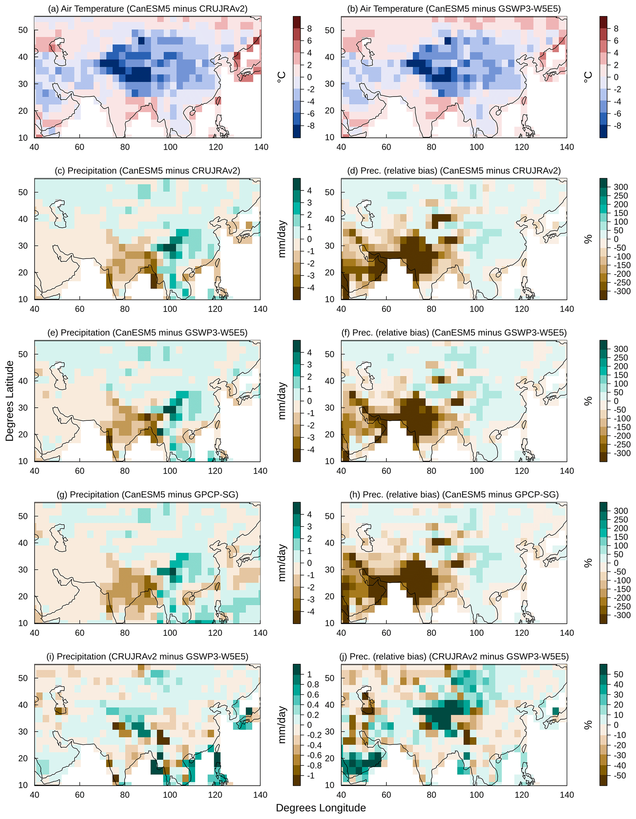
Figure 21 Bias in CanESM5.0 simulated annual-mean surface air temperature and precipitation compared to the CRU-JRA, GSWP3, and GPCP datasets over the southeastern Asian region for the 1970–2014 period. Panels (a) and (b) show the bias in CanESM5 simulated near-surface air temperature compared to the CRU-JRA and GSWP3 datasets, respectively. Panels (c) through (h) show the absolute and relative bias in CanESM5.0 simulated precipitation compared to the CRU-JRA, GSWP3, and GPCP datasets. Panel (i) and (j) show the absolute and relative precipitation differences between the CRU-JRA and GSWP3 datasets.

Figure 21 shows the biases in simulated annual mean temperature and precipitation from CanESM5.0 compared to the CRU-JRA, GSWP3 and Global Precipitation Climatology Project (GPCP) datasets averaged over the 1970–2014 period. Note that the CRU-JRA and GSWP3 are meteorological datasets that are available only over land (and are used to drive CLASSIC offline, as described above), while GPCP is an observation-based precipitation dataset and is available for the whole globe. CanESM5.0 shows a large cold bias over the Himalayan region (around −4 to −5 ^∘C) compared to both CRU-JRA and GSWP3 datasets (Fig. 21a, b) as mentioned earlier, and this cold bias extends into eastern China. Panels (c) through (h) of Fig. 21 show the absolute and relative bias in simulated CanESM5.0 precipitation compared to the CRU-JRA, GSWP3, and GPCP datasets. Overall, the bias in CanESM5.0 precipitation is similar compared to all observation-based datasets. The relative bias is largest over India. The coarse T63 spatial resolution (∼2.8^∘) of CanESM5.0 implies that topography is not well resolved, and high mountain peaks are not well represented. This is consistent with higher-than-observed moisture being advected over the Himalayas by the eastward surface winds in this region (Fig. 11 of Swart et al., 2019b), leading to too little precipitation over India and too much over eastern China. This leads to a warm temperature bias over India (Fig. 3) during the JJA monsoon season. In a similar way, CanESM5.0 precipitation is biased low over the Amazonian region and biased high over the Andes mountains (Fig. A5) because higher than observed advected moisture from the Atlantic Ocean makes its way over the Andes, given the westward surface winds in this region, and the low precipitation over the Amazonian region leads to a warm temperature bias there (Fig. 3).

The cold bias over the Himalayan region is not unique to CanESM5.0 and is seen in other ESMs. Lalande et al. (2021) analyze temperature and snow biases in CMIP6 models, including CanESM5.0, over the same region and find that the multi-model mean temperature from 26 models is biased cold by 1.9 ^∘C associated with a 12 % overestimation of snow cover compared to a satellite-based dataset. Lalande et al. (2021) find that although higher-than-observed precipitation is the cause of the higher snow amounts and consequently higher surface albedo in most models in the region, other factors including snow fraction parameterization also play a role. Hence the Himalayan cold bias can be regarded as a community-systemic issue, although it is relatively large in CanESM5.0 (∼4–5 ^∘C; Fig. 21a, b) compared to the Lalande et al. (2021) CMIP6 multi-model mean Himalayan cold bias of ∼2^∘.

In summary, it appears that positive precipitation bias over the Himalayan region, which is likely caused by the coarsely resolved topography of the model, combined with the lack of a snow fraction parameterization that takes into account the effect of topography, leads to a large accumulation of snow as the model spins up under pre-industrial forcing. The higher snow amounts and the resulting increase in surface albedo lead to a cold temperature bias over the Himalayan region. The next version of CanESM is expected to have a nominal spatial resolution of 1^∘ for its atmosphere and land components, and it is expected that biases related to unresolved topography will be reduced in magnitude and spatial extent. Work is also currently underway to evaluate an improved snow fraction parameterization in the CLASSIC land model.

6 Summary and discussion

In this paper, we have documented efforts within the CCCma, the group leading the development of the Canadian Earth System Model, to systematically monitor, document and eventually resolve model biases, through initiation of the Analysis for Development (A4D) activity. We have reported results from this activity, which includes two variants (p1 and p2) of a new CanESM version, CanESM5.1, featuring several improvements compared to CanESM5.0. A number of deep-dive analyses on specific model biases have provided insights into their sources and potential resolutions in future CanESM versions.

To aid in the analysis of these biases, three broad categories of model issues were employed to help identify their sources: version-specific, model-systemic, and community-systemic issues (Sect. 2). The majority of biases found in CanESM5.0 and CanESM5.1 appear to be version-specific issues (i.e., particular to this latest major model version). These include the occurrence of spurious spikes in stratospheric temperature and dust, as well as tropospheric dust storms (Sect. 5.1, an issue that was resolved in CanESM5.1); degraded ENSO relative to its predecessor CanESM2/CanCM4 (Sect. 5.2.1, a bias that was reduced in CanESM5.1-p2); a high EffCS (Sect. 5.2.2, reduced by about 30 % in CanESM5.1-p2); excessive North Atlantic sea ice during late winter (Sect. 5.3.1); and too few sudden stratospheric warmings (Sect. 5.3.3). Model-systemic issues include the cold winter bias above sea ice (Sect. 5.3.2) and the Himalayan cold bias (Sect. 5.3.4). Community-systemic biases – i.e., biases in CanESM that resemble those seen in multiple CMIP models – include the excessive westward extension of SST anomalies (Sect. 5.2.1) and the Himalayan cold bias (Sect. 5.3.4). Community-systematic errors are important to identify because their potential influence on multi-model analyses cannot easily be removed by averaging across a multi-model ensemble (since many models share these same errors); hence, documenting them is important for informing users of the output of these models.

In general, the nature of any model bias can be further understood in terms of it being parametric or structural. Parametric issues are dependent on parameter values primarily associated with physical parameterizations, while structural ones are dependent on model formulation (essentially, everything else). For version-specific biases, the question of whether they are dependent on model tuning is highly relevant. Model-systemic biases suggest structural origins but parametric explanations might also be relevant if a particular tuning approach has impacted multiple model versions. For community-systemic biases, it is almost certainly the case that their origins are structural. The p2 variant of CanESM5.1 (Sect. 3.2.1) was an attempt to gain some insight into the parametric nature of biases present in the p1 variant of CanESM5.1 (and in CanESM5.0, given its strong similarity to CanESM5.1-p1). Ideally, one would span all parameter values to gauge such sensitivity. At the CCCma, we have begun using a more objective tuning approach (e.g., Hourdin et al., 2017) that uses history matching methods based on Bayesian statistics to determine suitable values for CanESM’s free physical parameters in finalizing model versions (Williamson et al., 2015, 2017). The application of this approach to parameter tuning spans all possible values of selected free parameters and so should be a valuable tool to identify the nature of model biases as either parametric or structural.

As the primary goal of A4D is to better support model development and provide a more objective path toward model versions with improved properties and behaviour, an essential component of A4D is an ongoing critical review of its effectiveness in meeting this goal. It is anticipated that the A4D effort will evolve based on the effectiveness of its initial implementation and due to the implementation of new technologies applied to model development (such as model tuning by history matching methods). While development of the next major version of CanESM is still at an early stage, it is expected to include substantial changes compared to CanESM5.0 and CanESM5.1, including the following: a new dynamical core; a new version of the ocean model, which includes a new sea-ice component; and a new ecosystem and land surface model. Such major changes will almost certainly alter the nature and sources of CanESM biases, presenting new and unique challenges to our model development efforts. By increasing focus on analysis that is specifically tailored to support model development, we have implemented structures and tools that will put us on a path to better meet these challenges.

Appendix A: Supplemental Figures

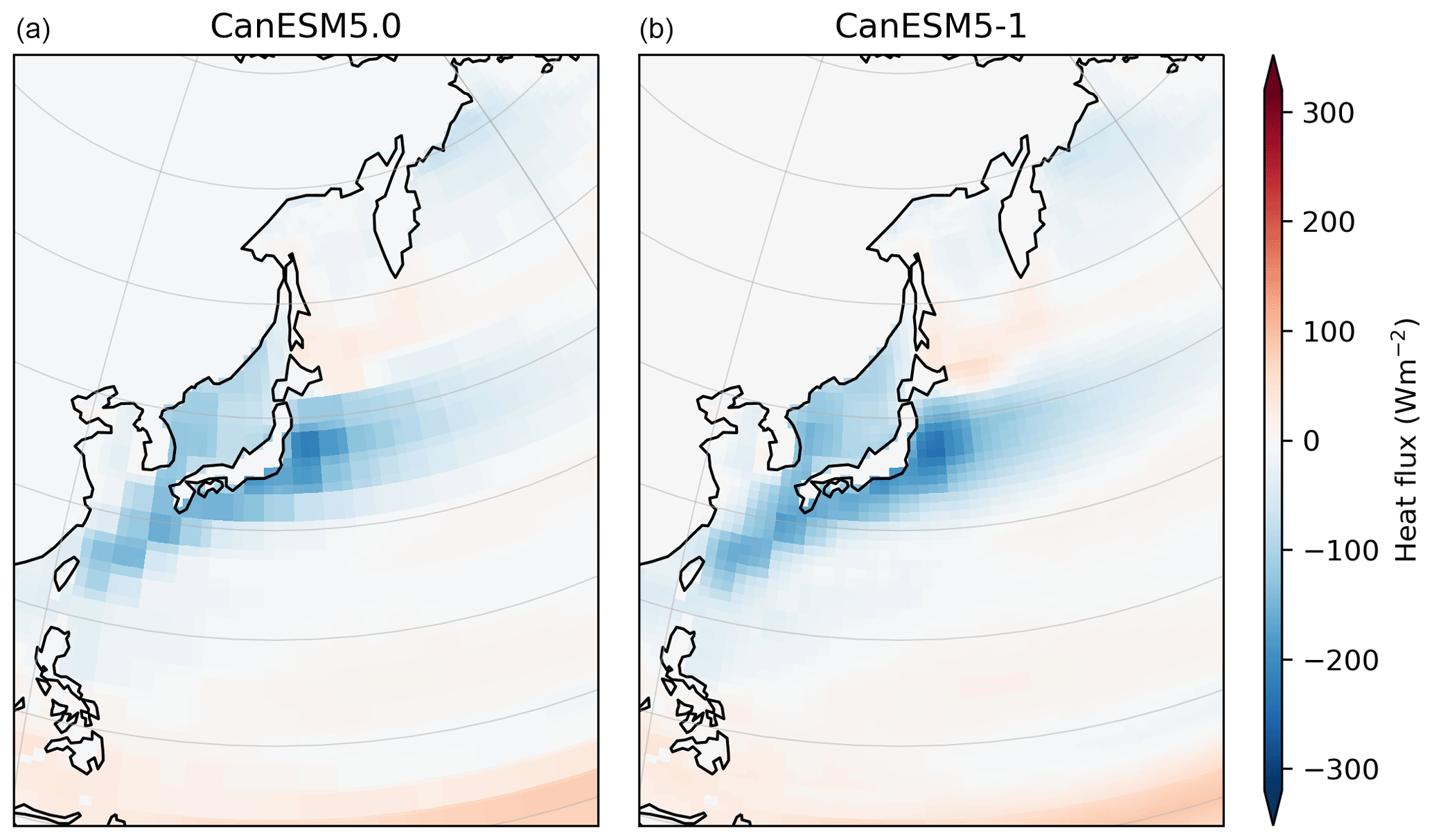
Figure A1 Net surface downward heat flux in CanESM5.0 (a) and CanESM5.1 (b) on the native ocean grid, over the vicinity of the Kuroshio Current. The ESMF conservative2 remapping method used in CanESM5.1 leads to a somewhat smoother field than seen in CanESM5.0, which uses the ESMF conservative remapping. The blockiness in the fields arises due to the much coarser resolution of the atmospheric grid ($\approx \mathrm{3}{}^{\circ }$), where the fluxes are computed, relative to the ocean grid (1^∘).

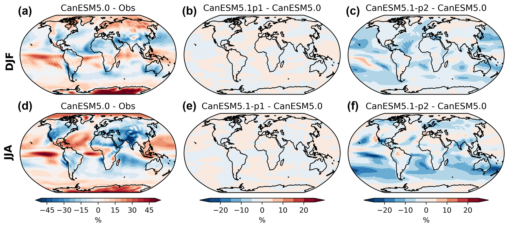
Figure A2 Same as Fig. 3 except for cloud fraction and the bias relative to International Satellite Cloud Climatology Project H series (ISCCP-H) satellite-based observations (Young et al., 2018) averaged over 1991–2010

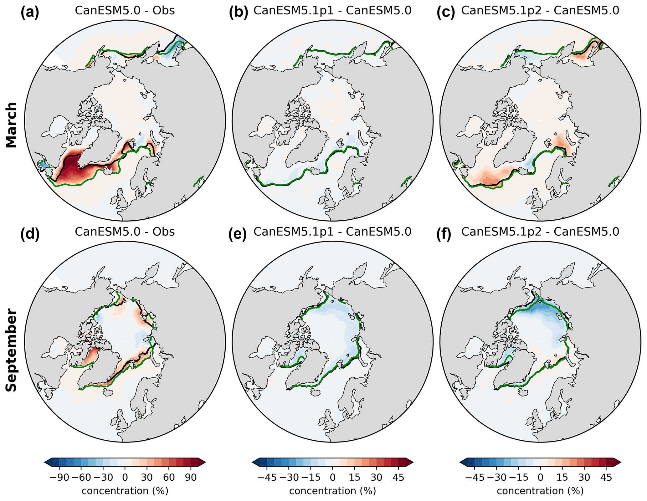
Figure A3 Same as Fig. 3 except for Arctic sea-ice concentration in March (a–c) and September (d–f), as well as sea-ice concentration from NSIDC as the observations. The ice edge (15 % sea-ice concentration contour) is indicated by green for CanESM5.0 in (a) and (d), CanESM5.1-p1 in (b) and (e), and CanESM5.1-p2 in (c) and (f). For comparison, the black contour indicates the ice edge for observations in (a) and (d) and for CanESM5.0 in (b), (c), (e), and (f).

The ice edge (15 sea ice concentration contour) is indicated by green for CanESM5.0 in (a), (d), CanESM5.1-p1 in (b), (e) and CanESM5.1-p2 in (c), (d). For comparison, the black contour indicates the ice edge in observations in (a), (d) and in CanESM5.0 in (b), (c), (e) and (f).

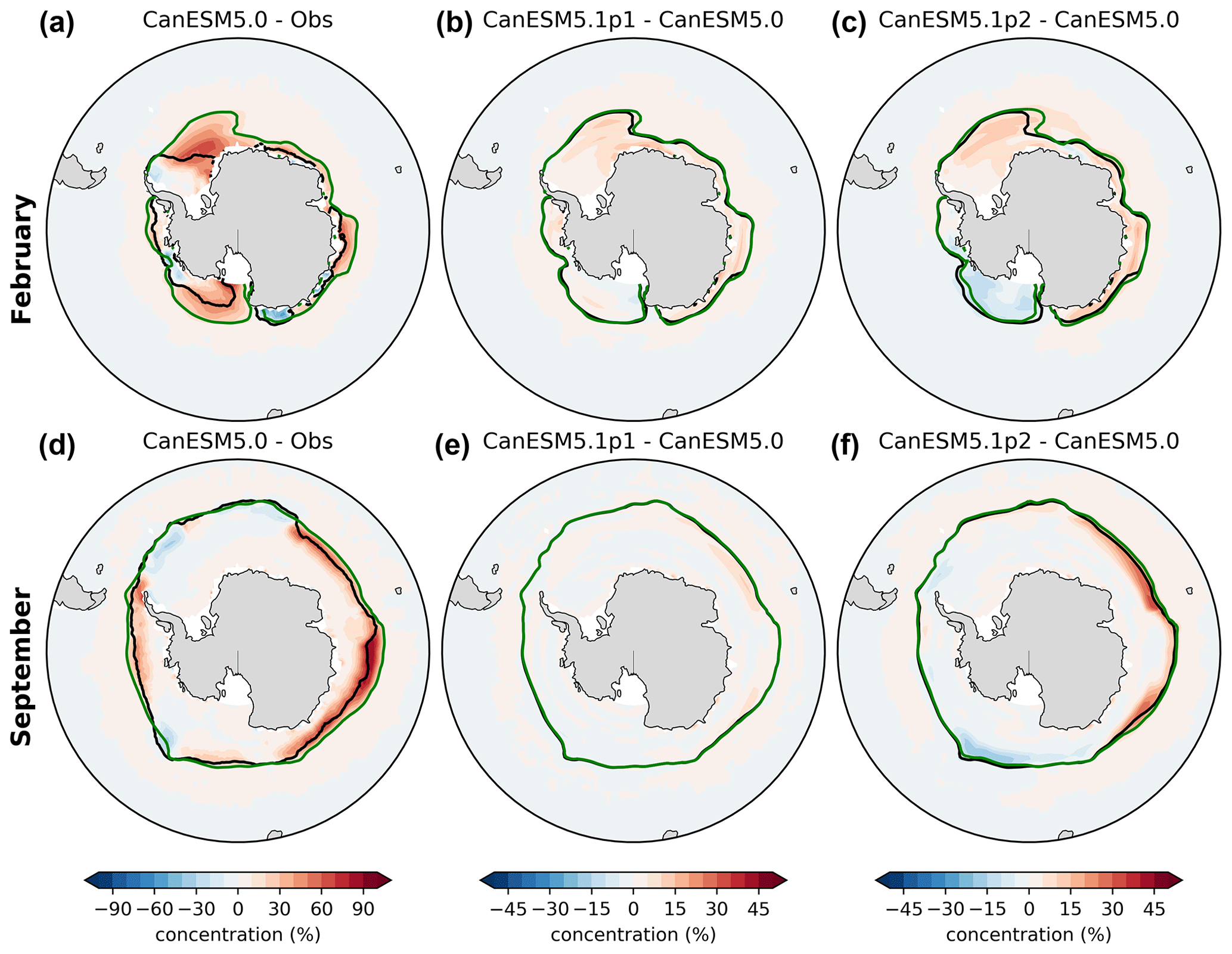
Figure A4 Same as Fig. A3 except for Antarctic sea ice in February (a–c) and September (d–f).

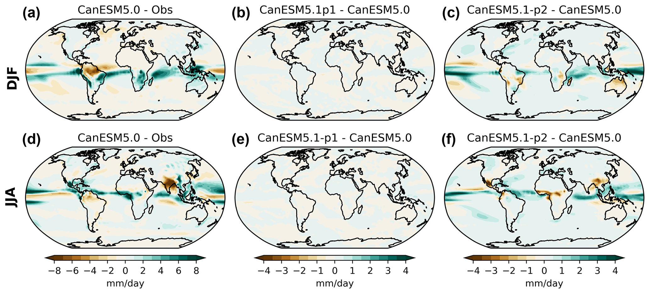
Figure A5 Same as Fig. 3 except for precipitation using GPCP as the observations.

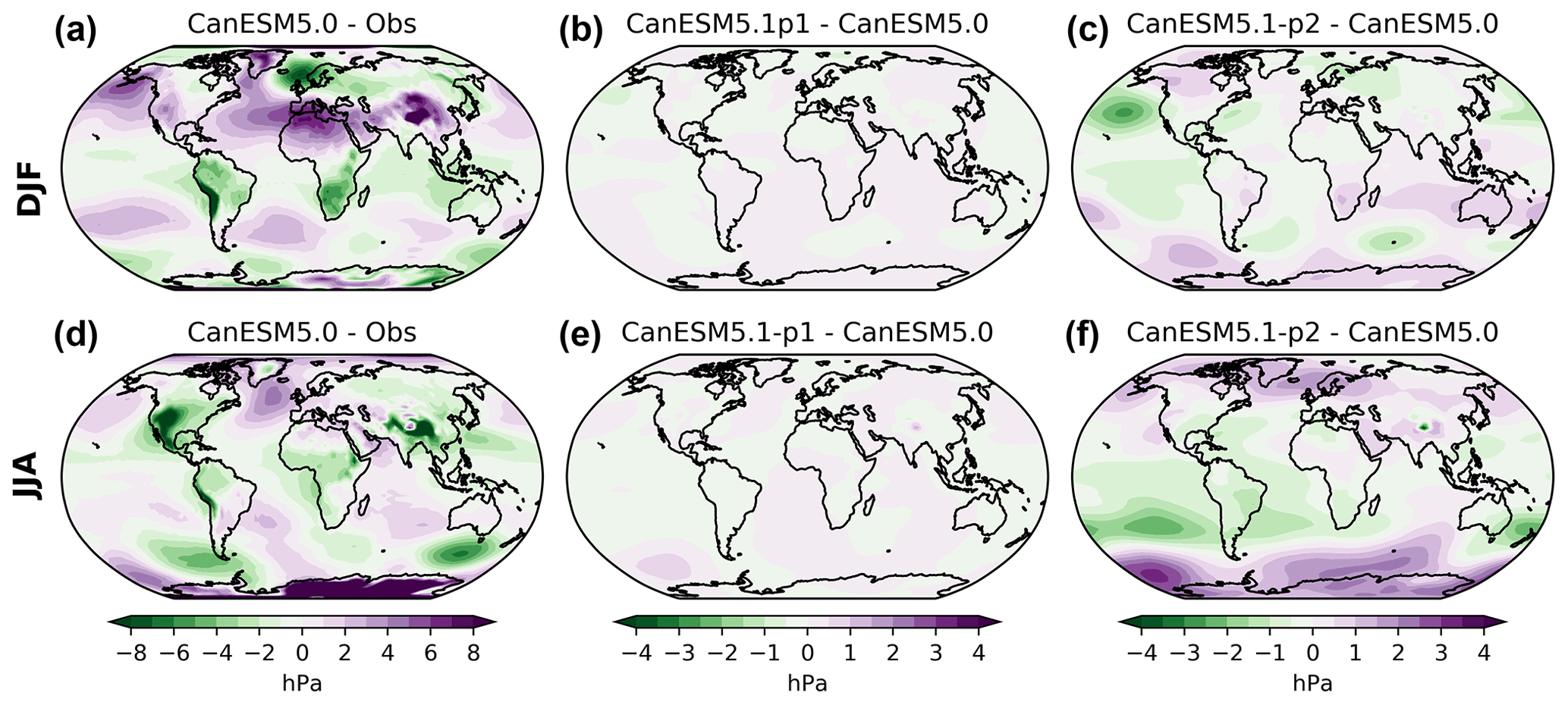
Figure A6 Same as Fig. 3 except for sea level pressure using ERA5 as the observations.

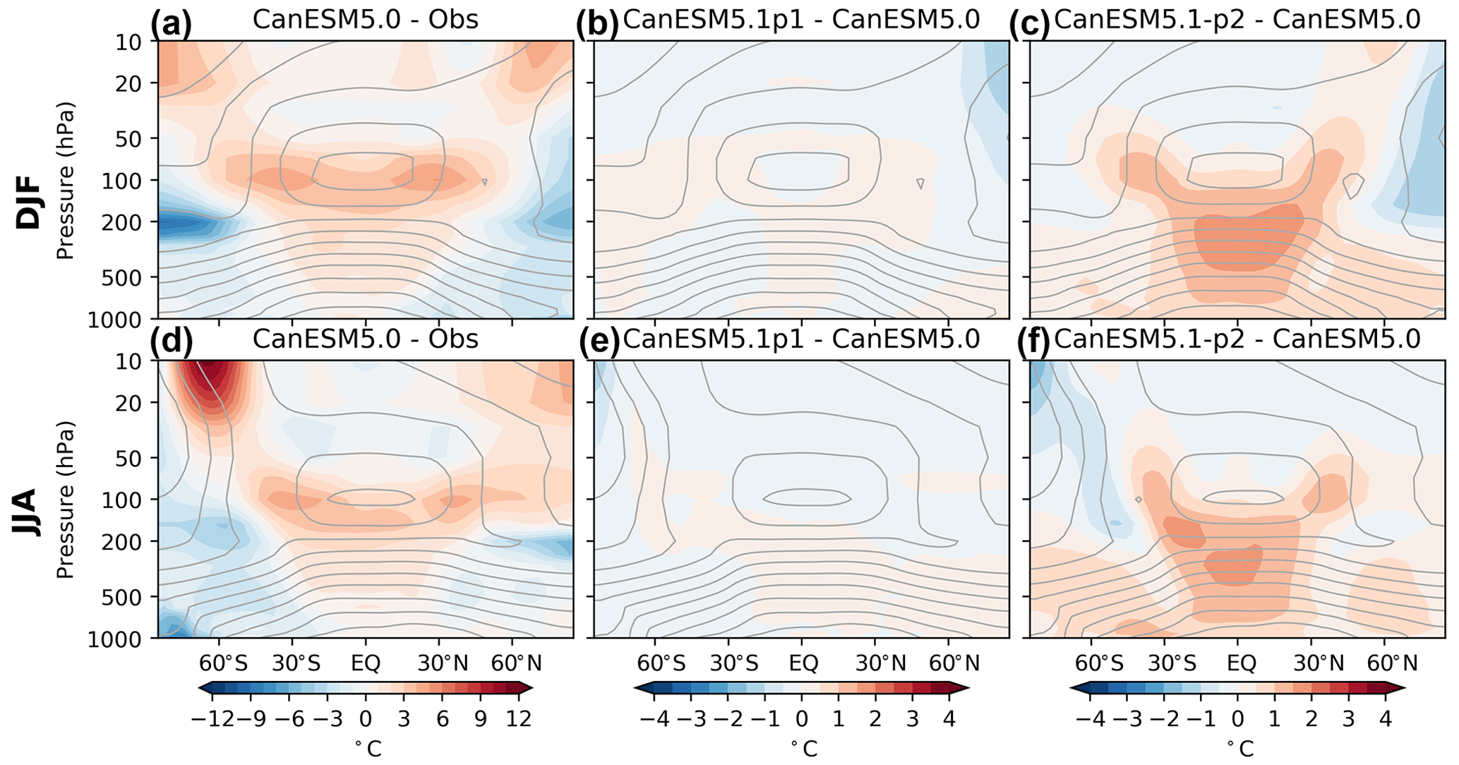
Figure A7 Same as Fig. 3 except for zonal mean temperature using ERA5 as the observations, with the contours representing the climatological zonal mean temperatures in CanESM5.0 (a, d), CanESM5.1-p1 (b, e) and CanESM5.1-p2 (c, f) (contour interval: 10 ^∘C).

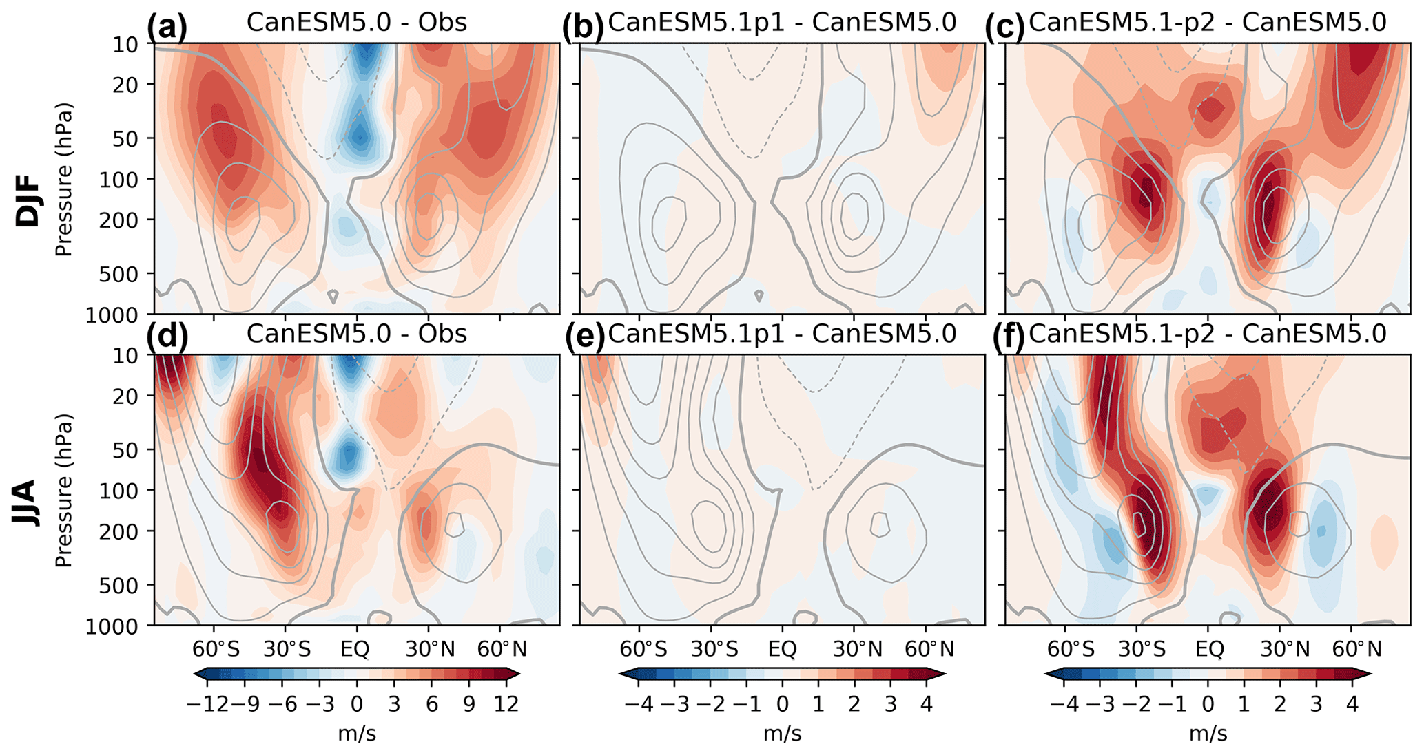
Figure A8 Same as Fig. 3 except for zonal mean zonal wind using ERA5 as the observations. The contours represent the climatological zonal mean temperatures in CanESM5.0 (a, d), CanESM5.1-p1 (b, e) and CanESM5.1-p2 (c, f). The contour interval is 10 m s⁻¹ with the thick solid line denoting the 0 m s⁻¹ contour.

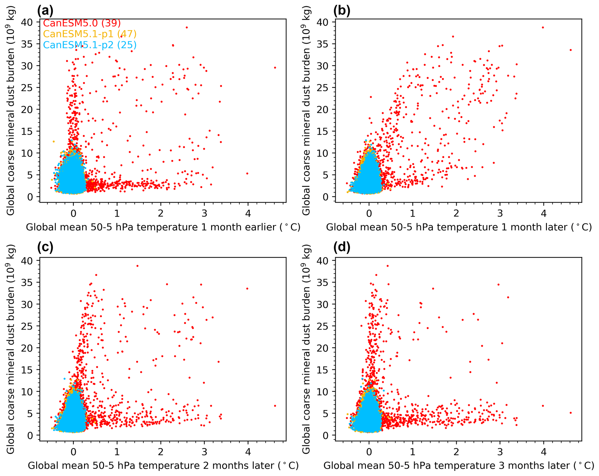
Figure A9 Total global coarse mineral dust burden versus unforced global mean lower-stratospheric temperature in (a) the previous month, (b) the next month, (c) the second month and (d) the third month (for all months and all ensemble members).

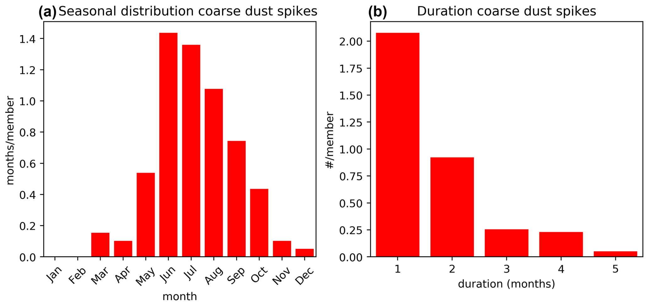
Figure A10 (a) Seasonal distribution and (b) histogram of the duration of the coarse mineral dust spikes with global burden that exceeds 12×10⁹ kg in CanESM5.0.

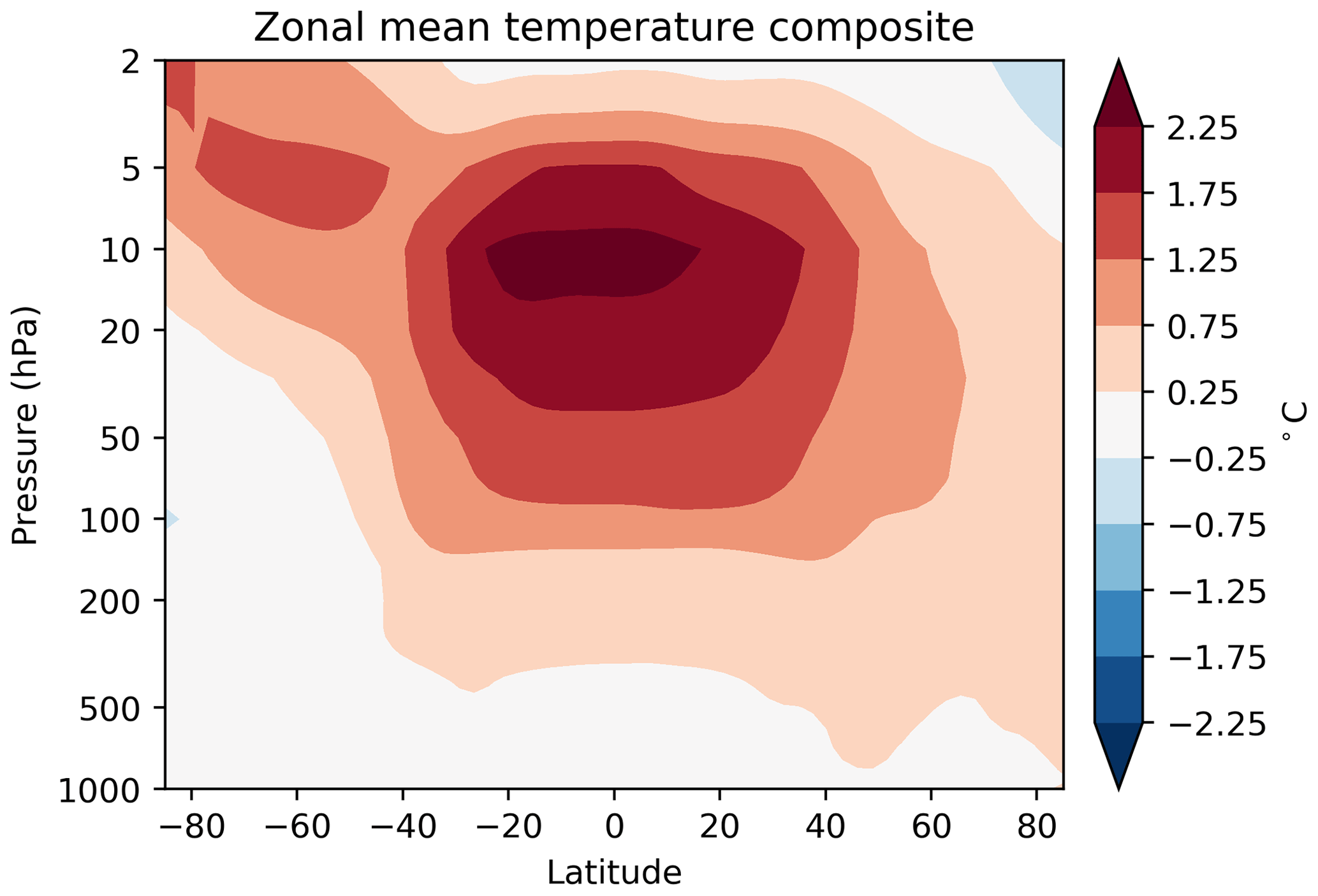
Figure A11 Zonal mean temperature anomaly composite of all months in with coarse mineral dust burden exceeding 12×10⁹ kg in CanESM5.0.

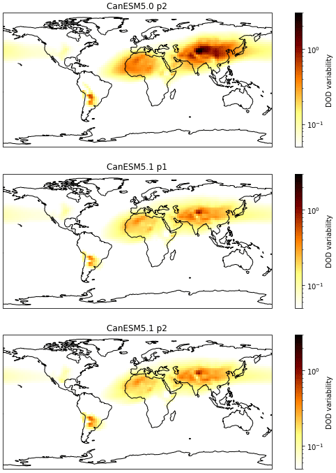
Figure A12 Typical variability in dust optical depth in CanESM versions CanESM5.0-p2, CanESM5.1-p1 and CanESM5.1-p2. For each ensemble member, variability is calculated as the standard deviation in dust optical depth over 2007–2014; maps show the ensemble mean of this variability. Note the logarithmic colour scale and the reduction in variability from CanESM5.0 to CanESM5.1.

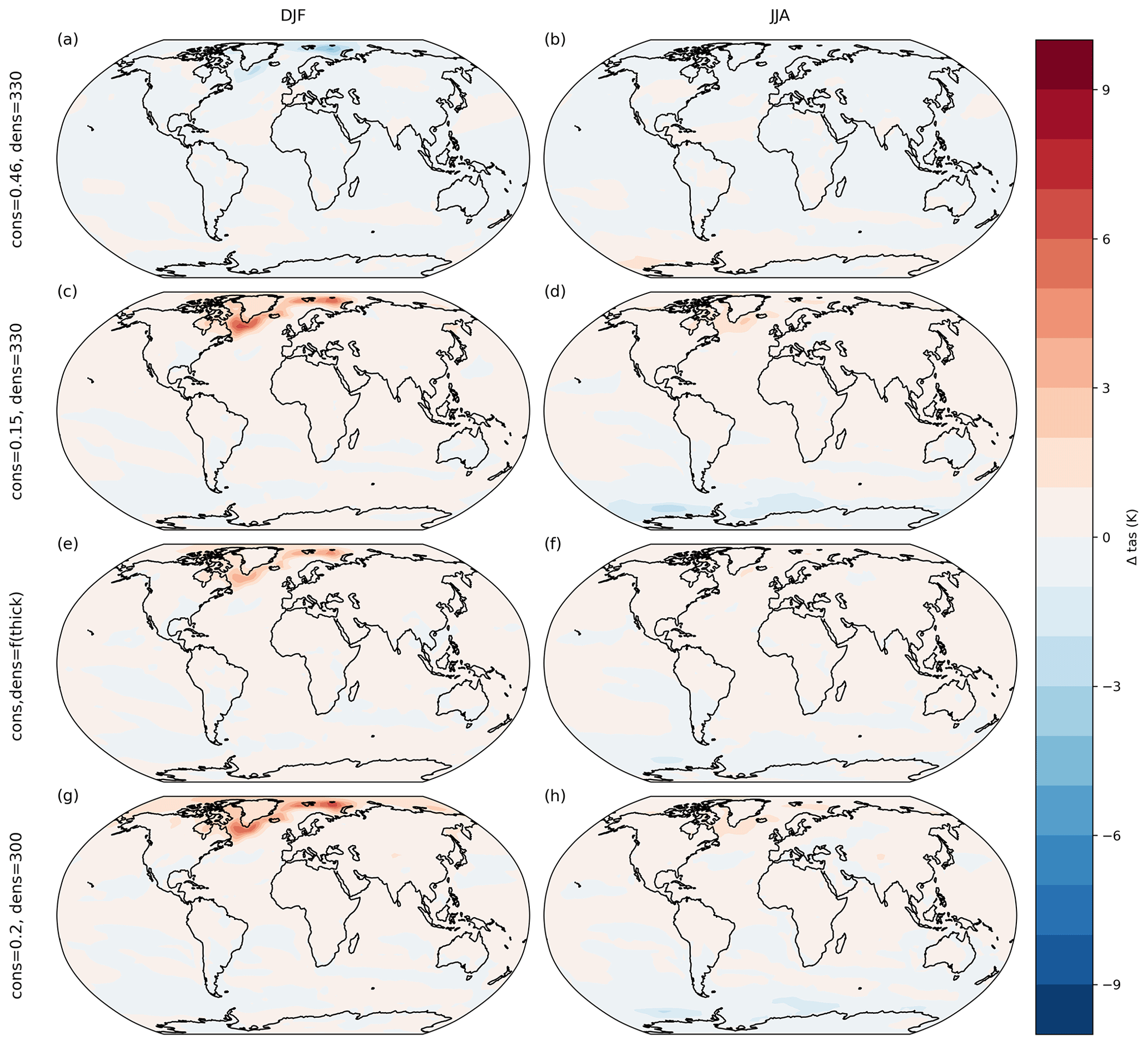
Figure A13 Surface air temperature anomalies, relative to the control experiment using default CanAM5 values (Table 3, first row), in the DJF (left column) and JJA (right column) seasons, for the experiments with altered snow conductivity and snow density listed in Table 3: experiments 4 (a, b), 3 (c, d), 2 (e, f), and 1 (g, h). Experiments 5 and 6 that alter the ice conductivity are not shown here but show even smaller anomalies than the other experiments.

Appendix B: Remotely sensed observations of aerosol optical depth

We here describe the remotely sensed observations of aerosol optical depth used for model evaluation in Sect. 5.1 and provide an overview of their strengths and limitations.

We use monthly-mean total AOD retrieved from the Moderate Resolution Imaging Spectroradiometer (MODIS; King et al., 2013), Multi-angle Spectral Radiometer (MISR; Diner et al., 1998), and Cloud-Aerosol LIdar with Orthogonal Polarization (CALIOP; Winker et al., 2009) instruments. MODIS and MISR are passive instruments, measuring only during the day, and CALIOP is a lidar sensor which measures during both day and night. There are two MODIS instruments, carried on the Aqua and Terra satellites, with equatorial overpass times of 10:30 and 13:30 LT (local time), respectively; we consider the products from these two sensors separately. MISR and CALIOP are single instruments. MISR is carried aboard Terra, with one of the MODIS instruments. CALIOP is aboard the Cloud-Aerosol Lidar and Infrared Pathfinder Satellite Observations (CALIPSO) satellite, which lagged Aqua by 1–2 min during the time period analyzed here; it has since been relocated to a lower-altitude orbit.

Generally, AOD retrieved from MODIS is higher than that from other satellites, while AOD from MISR and CALIPSO is lower than other satellites, when comparing with other datasets that are available for shorter periods of time (Vogel et al., 2022a). The spread between MODIS and MISR/CALIPSO can thus be taken as an approximate estimate of the overall uncertainty in observed AOD. For CALIPSO, we include results for both daytime, cloud-free conditions (“CALIPSO CloudFreeDay”) and day-night averaged, all-sky conditions (“CALIPSO AllSkyDayNight”).

The retrieval of optical depth of dust is more challenging than total optical depth, because it requires additional information on particle size and/or shape in order to distinguish dust optical depth from the contributions of other aerosol types. MODIS and MISR do not provide dust products. CALIOP optical depths are published for dust and polluted dust categories, but these are separate classifications (the former refers to clean dust only, and the latter refers to dust mixed with urban pollution or biomass burning smoke), and there is no estimate of the total dust optical depth (Omar et al., 2009). Here we use the dust classification but emphasize that it is an underestimate of the total contribution from mineral dust. We augment these observations with dust optical depths from Song et al. (2021) (ACROS-MODIS and ACROS-CALIPSO, derived from MODIS and CALIPSO data, respectively), Gkikas et al. (2020) (MIDAS, derived from MODIS data), and Voss and Evan (2019) (Voss+2019, derived from MODIS data).

Appendix C: Supplementary material on North Atlantic biases

In the coupled modelling system, we have explored three hypotheses regarding the origin of the biases:

1. Issues in sea-ice thermodynamics or coupling encourage excessive ice growth and resulting SSS/SST biases.

2. Runoff bias impacts SSS and enhances stratification, reducing convection and enabling ice growth.

3. Atmospheric circulation bias impacts ocean tracer transport and surface properties.

As a test of the sensitivity to sea-ice thermodynamics, experiments 1 and 2 from Table 3, which adjust snow density and thermal conductivity within their uncertainty ranges, were carried into the historical period (and are otherwise identical to CanESM5 historical runs). Using a lower specific density and conductivity for snow (10 % and 35 % lower, respectively; experiment 1 settings from Table 3) does reduce the sea-ice bias but does not remove it or even recover a state comparable to CanESM2 (Fig. 16d). Variable snow density and conductivity (experiment 2 settings from Table 3) lead to an even smaller improvement (Fig. 16c).

River runoff in CanESM5 is derived from the CLASS land surface model, wherein the precipitation minus evaporation (P − E) residual is routed downhill to the coast and input as runoff where the atmospheric land fraction falls below 50 % (Swart et al., 2019b). This runoff field is then conservatively remapped in the coupler from the roughly 3^∘ atmospheric physics grid to the nominally 1^∘ ORCA1 tripolar grid. No further adjustment is undertaken. Due to the resolution difference between the models, this procedure effectively leads to runoff being distributed over several ocean grid cells away from the coast. In addition, the runoff magnitude can be biased by the P − E field in the atmospheric model. To test whether the amount or distribution of runoff in CanESM5 lead to the sea-ice biases, we did an experiment where the CLASS-based runoff was ignored, and the observationally based runoff from the OMIP experiment was read from file instead. This ultimately had little impact on the sea-ice bias (Fig. 16e).

Finally, synoptic-scale atmospheric circulation biases over the North Atlantic could play a role by influencing the subpolar ocean gyre. Climatological sea-level pressure in CanESM5.0 shows an Icelandic Low that is displaced northeast relative to observations, and an over-expressed gradient between the Icelandic Low and the Azores High (Fig. 15h). Similar biases exist in the AMIP mode (not shown), suggesting that this is a feature of the atmospheric model and not of the coupled climate. The wind stress associated with these pressure gradients would encourage a geostrophic oceanic circulation comprising a North Atlantic Current that remains coherent over the basin and extends the subpolar gyre too far to the east. This would imply that warm, salty tropical waters that should be delivered to the Labrador Sea instead traverse a much longer distance, losing heat to the atmosphere and dissipating within the broader North Atlantic basin. In turn, this would reduce the heat and salt flux into the Labrador Sea, thus making it more susceptible to freezing over and high stratification.

Testing such a hypothesis is a challenge. What we have done is to run coupled historical experiments where vorticity and divergence in the atmospheric model are spectrally nudged at synoptic length scales (T21 and coarser) toward the ERA5 reanalysis. The results from these experiments show a strong reduction in the Labrador Sea sea-ice bias early on, but this improvement fades with time since the onset of the nudging and leads to only modest improvement when considered over a 30-year period (Fig. 16f). The challenge with interpreting these experiments is that the introduction of nudging perturbs the model climate. Hence the model is not equilibrated, and over time the wind nudging drives the overall climate colder, making conditions more favourable to the return of the sea-ice bias. In future, we plan to derive stationary bias corrections from these nudging runs and use these to establish equilibrated climate states to test this hypothesis. Similarly, OMIP-like ocean-only experiments that systematically change out only the observed wind stress for the CanESM5 wind stress are not definitive: the specification of other surface forcing from observations (e.g., surface air temperature and SSS) carries with it the imprint of observed sea-ice distributions, and the lack of coupled feedbacks suppresses the true effect that wind stress bias would have in the coupled model.