IMEX_SfloW2D v2: a depth-averaged numerical flow model for volcanic gas–particle flows over complex topographies and water

We present developments to the physical model and the open-source numerical code IMEX_SfloW2D (de' Michieli Vitturi et al., 2019). These developments consist of a generalization of the depth-averaged (shallow-water) fluid equations to describe a polydisperse fluid–solid mixture, including terms for sedimentation and entrainment, transport equations for solid particles of different sizes, transport equations for different components of the carrier phase, and an equation for temperature/energy. Of relevance for the simulation of volcanic mass flows, vaporization and entrainment of water are implemented in the new model. The model can be easily adapted to simulate a wide range of volcanic mass flows (pyroclastic avalanches, lahars, pyroclastic surges), and here we present its application to transient dilute pyroclastic density currents (PDCs). The numerical algorithm and the code have been improved to allow for simulation of sub- to supercritical regimes and to simplify the setting of initial and boundary conditions. The code is open-source. The results of synthetic numerical benchmarks demonstrate the robustness of the numerical code in simulating transcritical flows interacting with the topography. Moreover, they highlight the importance of simulating transient in comparison to steady-state flows and flows in 2D versus 1D. Finally, we demonstrate the model capabilities to simulate a complex natural case involving the propagation of PDCs over the sea surface and across topographic obstacles, through application to Krakatau volcano, showing the relevance, at a large scale, of non-linear fluid dynamic features, such as hydraulic jumps and von Kármán vortices, to flow conditions such as velocity and runout.

1 Introduction

In the past decades, the development of numerical models for geophysical mass flows and their application to hazard assessment has seen a rapid growth. Better understanding of the physics governing such flows has enabled development of more accurate models while a tremendous increase in computational resources has made increasingly high-resolution numerical simulations possible. Despite these advances, for some applications, there is still a need for simplified and fast, yet reliable, models. This is true, for example, for forecasting and hazard quantification purposes, where a probabilistic approach generally requires a large number (thousands or more) of simulations in a relatively short time frame.

For a large class of geophysical mass flows, characterized by having the horizontal length scale much greater than the vertical one, it is possible to reduce the dimensionality of the problem (and thus the computational cost of its numerical solution) by adopting the approach of so-called shallow-water equations. The shallow-water equations are a set of partial differential equations that describe fluid flow problems, originally introduced by Adhémar Jean Claude Barré de Saint-Venant, and are obtained by the averaging of flow variables over its thickness, thus reducing the model complexity (Pudasaini and Hutter, 2007; Toro, 2013). Shallow-water equations have been applied successfully to tsunamis (Fernández-Nieto et al., 2008), atmospheric flows (Zeitlin, 2018), storm surges (Von Storch and Woth, 2008), landslides and debris flows (Iverson and Denlinger, 2001; Denlinger and Iverson, 2001), snow and rock avalanches (Bartelt et al., 1999; Christen et al., 2010), and planetary flows (Iga and Matsuda, 2005). In the volcanological field, shallow-water equations have been applied to umbrella cloud spreading (Johnson et al., 2015; de' Michieli Vitturi and Pardini, 2021), lahars (Fagents and Baloga, 2006; O'Brien et al., 1993), pyroclastic density currents (Pitman et al., 2003; Patra et al., 2005; Capra et al., 2008; Calabrò et al., 2022; Kelfoun et al., 2009; de' Michieli Vitturi et al., 2019; Shimizu et al., 2017a) and lava flows (Costa and Macedonio, 2005; Biagioli et al., 2021; Hyman et al., 2022).

Another common feature of most geophysical flows is that they are multiphase flows, with a continuous carrier phase (gas or liquid) and a solid dispersed phase. For the numerical modelling of such multiphase flows, two main approaches can be adopted, with the solid phase treated as a continuum (Eulerian approach) or as discrete elements for which the equations of motion are solved (Lagrangian approach). The latter approach is better suited for low particle concentrations and when the particle relaxation time, quantified by the inertial effect of particles, is much smaller than the characteristic time of collisions between particles (Dufek, 2015; Neri et al., 2022). For the volcanological applications of interest here (dilute pyroclastic density currents, or dilute PDCs), the flow can be highly turbulent, favouring particle collisions, and thus the continuum approach is appropriate. Most of these flows can be described and modelled using the full 3D transient multiphase Navier–Stokes equations, but, since the numerical three-dimensional calculation is still very costly, it makes sense to reduce the equations for calculations with simpler flow conditions. In particular, for currents where turbulent mixing is large enough to maintain vertically uniform concentration, shallow-water models provide a good approximation (Bonnecaze et al., 1993). This approach can still be used for vertically stratified flows, but it is necessary to introduce appropriate correction factors into the equations, generally based on a simplifying assumption of well-developed and stationary vertical profiles and yet not easy to calculate explicitly (Biagioli et al., 2021; Keim and de' Michieli Vitturi, 2022).

In this work, we present a new version of IMEX-SfloW2D (de' Michieli Vitturi et al., 2019), a depth-averaged model originally developed for the simulation of pyroclastic avalanches, i.e. a type of granular flow characterized by relatively thin layers at high particle concentration (10–50 vol  %). Similarly to other codes used in volcanological research and applications such as VolcFlow (Kelfoun and Druitt, 2005), TITAN2D (Pitman et al., 2003; Patra et al., 2005) and SHALTOP (Bouchut and Westdickenberg, 2004; Mangeney et al., 2007), IMEX-SfloW2D is a shallow-water-equation model based on depth averaging, obtained by integrating the full 3D equations along the vertical dimension. With respect to the original version of the model (de' Michieli Vitturi et al., 2019), where the granular mixture was described as a single-phase mono-disperse granular fluid ignoring the presence of the interstitial gas, here the formulation and the equations have been generalized to a fluid–solid mixture, also adding sedimentation and entrainment terms, transport equations for the solid particles of different sizes, transport equations for different components of the carrier phase, and an equation for temperature/energy.

The model framework is general, and, by changing the constitutive equations defining phase properties and flow rheology, it is possible to simulate a variety of geophysical flows. However, in this paper we focus our attention on the modelling of PDCs, i.e. flows of gas and pyroclasts (fragments of volcanic rocks produced by explosive fragmentation), and in particular dilute PDCs, which are characterized by densities of less than 10 kg m⁻³ (roughly corresponding to a particle volume fraction of less than approximately 0.01). This hypothesis allows us to neglect the influence of particle–particle friction and the internal stress tensor.

Dilute PDCs can form in relation to several volcanic behaviours (Valentine, 1987; Branney and Kokelaar, 2002; Sulpizio et al., 2014; Dufek et al., 2015), including the collapse of Plinian and Vulcanian columns and the explosive fragmentation of a lava dome or cryptodome (Sigurdsson et al., 2015). Irrespective of the generating mechanism, dilute PDC propagation regimes can be characterized by the flow Richardson number (Ri), expressing the ratio between the potential energy and the kinetic energy available for mixing or, in other terms, the ratio between the relative celerity of surface waves and the velocity of the flow (Chow, 1959). Dilute PDCs may propagate as either subcritical (Ri>1) or supercritical (Ri<1) flows (Bursik and Woods, 1996), and they can also experience transitions from one regime to the other. For supercritical flows, where the speed of the flow is greater than the speed of gravity waves, entrainment is significant and the runout distance tends to be shorter. As large amounts of ambient air are entrained into the flow, ash particles elutriate to form a coignimbrite column (Bursik and Woods, 1996; Engwell et al., 2016). Conversely, subcritical flows, where the velocity of the flow is low enough for internal waves to propagate in either direction, have negligible entrainment and tend to have longer runout distances. On par with entrainment, sedimentation exerts a major role in controlling the rate of change of the flow bulk density and, hence, its existence. Indeed, dilute PDCs, as any other density current (e.g. turbidity currents), exist until there is a positive density contrast with the ambient in which they flow. If sufficient air is entrained or a sufficient quantity of particles are lost by sedimentation, then the density falls below that of the ambient air and a buoyant liftoff occurs. The capability of dilute flows to overcome topographic barriers, and consequently the sedimentation regimes, also depends on the Richardson number (Woods and Wohletz, 1991; Woods et al., 1998). For these reasons, an accurate description of these regimes is mandatory for a model of dilute PDCs, both in the definition of the equations and in their numerical discretization and solution.

In this work, Sects. 2 and 3 are devoted to the presentation of the new physical model for dilute PDCs based on the shallow-water approximation. The new model extends previous similar models by describing a polydisperse fluid–solid mixture with sedimentation and entrainment terms, transport equations for the solid particles of different sizes, transport equations for different components of the carrier phase, and an equation for temperature/energy. Moreover, it accounts for the potential vaporization of liquid water and entrainment of water vapour into the current. Section 4 summarizes the main aspects of the numerical algorithm, with emphasis on those details that are relevant for resolving the sub- and supercritical transitional regimes. We devote Sect. 5 to the application of the model to one-dimensional literature benchmark tests (Delestre et al., 2013) in order to show the capability of the code to properly simulate the different flow regimes. For supercritical conditions, we also present two 2D test cases, derived from Engwell et al. (2016). These tests show that the steady conditions reached by the simulation after the initial transient phase correspond to those obtained with the 1D steady model presented in Engwell et al. (2016) and based on Bursik and Woods (1996). Finally, in Sect. 6 the model is applied to Krakatau volcano, with input parameters informed by the 1883 eruption. This is an original study on the propagation of PDCs over water, with a complex 3D topography and display of complex super- to subcritical regime transitions, well representing the complexity of PDC dynamics in real cases. For this example, a 30 m SRTM DEM of the area is used, which allows us to simulate the effects of real topographic obstacles on the flow propagation and understand how they control the flow regime.

Most of the examples presented in this work, as well as the source code, can be freely downloaded from the model repository at https://github.com/demichie/IMEX_SfloW2D_v2 (last access: 9 October 2023). The GitHub repository also contains pre- and post-processing Python scripts, both general and specific for the included examples. The repository and the codes (Fortran main code and Python utility scripts) are compliant with the set of standards defined by the European Open Science Cloud (EOSC) Synergy (Software Quality Assurance as a Service, SQAaaS), which assigned, through Quality Assessment & Awarding (QAA), an SQAaaS gold badge. The compiled code is also available as a Docker container at the following link: https://hub.docker.com/r/demichie/imex_sflow2d_v2 (last access: 9 October 2023).

2  The physical model

We present here the equations adopted to describe a gas–particle flow with temperature-dependent mixture density, under the assumptions that the flow propagates at atmospheric pressure and that the effects of compressibility are negligible. In addition, we adopt a physical formulation based on depth averaging of the flow variables, which is appropriate for shallow flows and is computationally less expensive than considering density and velocity variation with depth.

Table 1 List of model variables with notation and units.

The model is based on the Saint-Venant equations (Pudasaini and Hutter, 2007; Toro, 2013), coupled with source terms describing the entrainment/loss of mass and frictional forces and enriched with an energy equation and with transport equations for different flow phases/components. In fact, we assume that the flow is a homogeneous mixture of a multi-component gas phase (for the applications presented in this work air and water vapour) and n_s dispersed solid phases. The density of the mixture ${\mathit{\rho }}_{\mathrm{m}}(x,y,t)$ is defined in terms of the volumetric fractions α_(⋅) and densities ρ_(⋅) of the components:

$$\begin{array}{}\text{(1)}& {\mathit{\rho }}_{\mathrm{m}}={\mathit{\alpha }}_{\mathrm{a}}{\mathit{\rho }}_{\mathrm{a}}+{\mathit{\alpha }}_{\mathrm{wv}}{\mathit{\rho }}_{\mathrm{wv}}+\sum _{i_{\mathrm{s}}=\mathrm{1}}^{n_{\mathrm{s}}}{\mathit{\alpha }}_{\mathrm{s},i_{\mathrm{s}}}{\mathit{\rho }}_{\mathrm{s},i_{\mathrm{s}}},\end{array}$$

where the subscript a denotes the air component; the subscript wv denotes the water vapour component; and the subscript s,i_s denotes the class $i_{\mathrm{s}}=\mathrm{1},\mathrm{\dots },n_{\mathrm{s}}$ of the solid phases. Each solid class is characterized by its diameter $d_{i_{\mathrm{s}}}$, density ${\mathit{\rho }}_{\mathrm{s},i_{\mathrm{s}}}$, and specific heat $C_{\mathrm{s},i_{\mathrm{s}}}$. For a full list of model variables and notation, please refer to Table 1.

Equations are written in global Cartesian coordinates, with x and y orthogonal to the z axis, parallel to gravitational acceleration $\mathit{g}=(\mathrm{0},\mathrm{0},g)$. We denote the flow thickness (parallel to the vertical z axis) with $h(x,y,t)$ and the horizontal components of the flow velocity with $u(x,y,t)$ and $v(x,y,t)$ (averaged over the vertical flow thickness). The flow moves over a topography $B(x,y,t)$, and we allow the topography to change with time (for example, by particle sedimentation).

Conservation of mass for the flow is calculated as follows:

$$\begin{array}{}\text{(2)}& \begin{array}{rl}{\displaystyle \frac{\partial {\mathit{\rho }}_{\mathrm{m}}h}{\partial t}}& +{\displaystyle \frac{\partial \left({\mathit{\rho }}_{\mathrm{m}}hu\right)}{\partial x}}+{\displaystyle \frac{\partial \left({\mathit{\rho }}_{\mathrm{m}}hv\right)}{\partial y}}\\ & =-\sum _{i_{\mathrm{s}}=\mathrm{1}}^{n_{\mathrm{s}}}\left[{\mathit{\rho }}_{\mathrm{s},i_{\mathrm{s}}}{S}_{\mathrm{s},i_{\mathrm{s}}}\right)]+{\mathit{\rho }}_{\mathrm{a}}{E}_{\mathrm{a}}+{\mathit{\rho }}_{\mathrm{wv},\mathrm{b}}{E}_{\mathrm{wv}},\end{array}\end{array}$$

where S_s is the volumetric rate of sedimentation of solid particles; E_a is the volumetric air entrainment rate from the atmosphere; and E_wv is the volumetric water vapour entrainment, which could occur for flows over waterbodies (sea or lakes). These rates are defined per unit surface area and thus have units of metres per second. The notation ρ_wv,b used here denotes the density of water vapour ingested into the flow, which is not that corresponding to flow temperature but boiling temperature.

Introducing the notation g^′ for the reduced gravity $g^{\prime }=\left[\right({\mathit{\rho }}_{\mathrm{m}}-{\mathit{\rho }}_{\mathrm{a}})/{\mathit{\rho }}_{\mathrm{m}}]g$, the equations for the momentum components are as follows:

$$\begin{array}{}\text{(3)}& {\displaystyle }\begin{array}{rl}& {\displaystyle \frac{\partial \left({\mathit{\rho }}_{\mathrm{m}}hu\right)}{\partial t}}+{\displaystyle \frac{\partial }{\partial x}}\left({\mathit{\rho }}_{\mathrm{m}}h{u}^{\mathrm{2}}+{\mathit{\rho }}_{\mathrm{m}}{g}^{\prime }{\displaystyle \frac{h^{\mathrm{2}}}{\mathrm{2}}}\right)+{\displaystyle \frac{\partial }{\partial y}}\left({\mathit{\rho }}_{\mathrm{m}}huv\right)\\ & =-{\mathit{\rho }}_{\mathrm{m}}{g}^{\prime }h{\displaystyle \frac{\partial B}{\partial x}}+F_x-u\sum _{i_{\mathrm{s}}=\mathrm{1}}^{n_{\mathrm{s}}}\left({\mathit{\rho }}_{\mathrm{s},i_{\mathrm{s}}}{S}_{\mathrm{s},i_{\mathrm{s}}}\right),\end{array}\text{(4)}& {\displaystyle }\begin{array}{rl}& {\displaystyle \frac{\partial \left({\mathit{\rho }}_{\mathrm{m}}hv\right)}{\partial t}}+{\displaystyle \frac{\partial }{\partial x}}\left({\mathit{\rho }}_{\mathrm{m}}huv\right)+{\displaystyle \frac{\partial }{\partial y}}\left({\mathit{\rho }}_{\mathrm{m}}h{v}^{\mathrm{2}}+{\mathit{\rho }}_{\mathrm{m}}{g}^{\prime }{\displaystyle \frac{h^{\mathrm{2}}}{\mathrm{2}}}\right)\\ & =-{\mathit{\rho }}_{\mathrm{m}}{g}^{\prime }h{\displaystyle \frac{\partial B}{\partial y}}+F_y-v\sum _{i_{\mathrm{s}}=\mathrm{1}}^{n_{\mathrm{s}}}\left({\mathit{\rho }}_{\mathrm{s},i_{\mathrm{s}}}{S}_{\mathrm{s},i_{\mathrm{s}}}\right),\end{array}\end{array}$$

where F_x and F_y represent the friction terms. Equations (3) and (4) are derived in the so-called hydrostatic approximation; i.e. the variation in momentum in the z direction is neglected and pressure is always hydrostatic. There are no terms associated with air and water vapour entrainment because they do not carry any horizontal momentum into the flow.

Density of the gas components is a function of the flow temperature T, which changes with entrainment of external air. In addition, part of the thermal energy of particles lost when the current travels over water produces steam which can be entrained in the flow. For this reason, with respect to the classical incompressible shallow-water equations, we also model the total energy budget of the flow, by solving the following equation for the total mixture energy (sum of internal and kinetic energies):

$$\begin{array}{}\text{(5)}& \begin{array}{rl}& {\displaystyle \frac{\partial }{\partial t}}\left[{\mathit{\rho }}_{\mathrm{m}}h\left(C_{\mathrm{v}}T+{\displaystyle \frac{\mathrm{1}}{\mathrm{2}}}\left(u^{\mathrm{2}}+v^{\mathrm{2}}\right)\right)\right]\\ & +{\displaystyle \frac{\partial }{\partial x}}\left(\left[C_{\mathrm{v}}T+{\displaystyle \frac{\mathrm{1}}{\mathrm{2}}}\left(u^{\mathrm{2}}+v^{\mathrm{2}}\right)+g^{\prime }{\displaystyle \frac{h}{\mathrm{2}}}\right]{\mathit{\rho }}_{\mathrm{m}}hu\right)\\ & +{\displaystyle \frac{\partial }{\partial y}}\left(\left[C_{\mathrm{v}}T+{\displaystyle \frac{\mathrm{1}}{\mathrm{2}}}\left(u^{\mathrm{2}}+v^{\mathrm{2}}\right)+g^{\prime }{\displaystyle \frac{h}{\mathrm{2}}}\right]{\mathit{\rho }}_{\mathrm{m}}hv\right)\\ & =-{\mathit{\rho }}_{\mathrm{m}}{g}^{\prime }h\left(u{\displaystyle \frac{\partial B}{\partial x}}+v{\displaystyle \frac{\partial B}{\partial y}}\right)\\ & -{\displaystyle \frac{\mathrm{1}}{\mathrm{2}}}\left(u^{\mathrm{2}}+v^{\mathrm{2}}\right)\sum _{i_{\mathrm{s}}=\mathrm{1}}^{n_{\mathrm{s}}}\left({\mathit{\rho }}_{\mathrm{s},i_{\mathrm{s}}}{S}_{\mathrm{s},i_{\mathrm{s}}}\right)-\sum _{i_{\mathrm{s}}=\mathrm{1}}^{n_{\mathrm{s}}}\left({\mathit{\rho }}_{\mathrm{s},i_{\mathrm{s}}}{C}_{\mathrm{s},i_{\mathrm{s}}}T{S}_{\mathrm{s},i_{\mathrm{s}}}\right)\\ & +C_{\mathrm{a}}{\mathit{\rho }}_{\mathrm{a}}{T}_{\mathrm{a}}{E}_{\mathrm{a}}+C_{\mathrm{wv}}{\mathit{\rho }}_{\mathrm{wv},\mathrm{b}}{T}_{\mathrm{b}}{E}_{\mathrm{wv}},\end{array}\end{array}$$

where C_v is the mass-averaged specific heat of the mixture; $C_{\mathrm{s},i_{\mathrm{s}}}$, C_a and C_wv are the specific heat of solid, air and water vapour, respectively; and T_a and T_b are the atmospheric air and water vapour temperatures before entrainment. In this equation, heat transfer by thermal conduction is neglected, as well as thermal radiation. The full derivation of the energy equation is presented in Appendix A2.

It is worth noting that the design of conservative and stable numerical schemes for the solution of Eqs. (2)–(5) requires some care. This is because the numerical solution of mass and momentum equations, even when these quantities are globally conserved, does not necessarily result in an accurate description of the mechanical energy balance of the shallow-water system (Fjordholm et al., 2011; Murillo and García-Navarro, 2013). In fact, many numerical schemes perform well in practice but they may have an excessive amount of numerical dissipation near shocks, preventing a correct energy dissipation property across discontinuities (which can arise even in the case of smooth topography). A quantification of the error in the conservation of mechanical energy is beyond the scope of this paper, also because the error is case dependent and the topography plays a crucial role, but the reader can refer to Arakawa and Lamb (1977), Arakawa (1997), Arakawa and Lamb (1981), and Fjordholm et al. (2011) for a comprehensive discussion of this issue. In general, to guarantee energy conservation in smooth regimes, it is desirable to design high-order schemes adding a minimal amount of numerical dissipation.

Numerical errors in the computation of the mechanical energy may also lead to errors associated with the mixture temperature obtained from the total mixture specific energy and the kinetic energy computed from mass and momentum equations. For this reason, in some cases, instead of the full energy equation as presented above, it is preferable to solve a simpler transport equation for the specific thermal energy C_vT:

$$\begin{array}{}\text{(6)}& \begin{array}{rl}& {\displaystyle \frac{\partial }{\partial t}}\left({\mathit{\rho }}_{\mathrm{m}}h{C}_{\mathrm{v}}T\right)+{\displaystyle \frac{\partial }{\partial x}}\left(C_{\mathrm{v}}T{\mathit{\rho }}_{\mathrm{m}}hu\right)+{\displaystyle \frac{\partial }{\partial y}}\left(C_{\mathrm{v}}T{\mathit{\rho }}_{\mathrm{m}}hv\right)=\\ & -\sum _{i_{\mathrm{s}}=\mathrm{1}}^{n_{\mathrm{s}}}\left({\mathit{\rho }}_{\mathrm{s},i_{\mathrm{s}}}{C}_{\mathrm{s},i_{\mathrm{s}}}T{S}_{\mathrm{s},i_{\mathrm{s}}}\right)+C_{\mathrm{a}}{\mathit{\rho }}_{\mathrm{a}}{T}_{\mathrm{a}}{E}_{\mathrm{a}}+C_{\mathrm{wv}}{\mathit{\rho }}_{\mathrm{wv},\mathrm{b}}{T}_{\mathrm{b}}{E}_{\mathrm{wv}}.\end{array}\end{array}$$

We remark that in this equation we neglect heating associated with friction forces. This term can be important for some applications where viscous forces are particularly large, for example lava flows, but is negligible for the applications presented in this work. It is also worth noting that the numerical solution of Eqs. (2)–(4) and (6) does not guarantee that the total energy is conserved. In the following part of this section, for simplicity, we use the temperature equation to demonstrate the writing of the system of equations in a more compact form and in the description of the numerical schemes, but for the applications presented in this work, the full energy equation is solved.

The quantities of solid particles and water vapour in the flow vary in space and time because of sedimentation and entrainment, respectively, and for this reason additional transport equations for the mass of n_s solid classes and the water vapour are also considered:

$$\begin{array}{}\text{(7)}& {\displaystyle }\begin{array}{rl}& {\displaystyle \frac{\partial {\mathit{\alpha }}_{\mathrm{s},i_{\mathrm{s}}}{\mathit{\rho }}_{\mathrm{s},i_{\mathrm{s}}}h}{\partial t}}+{\displaystyle \frac{\partial \left({\mathit{\alpha }}_{\mathrm{s},i_{\mathrm{s}}}{\mathit{\rho }}_{\mathrm{s},i_{\mathrm{s}}}hu\right)}{\partial x}}+{\displaystyle \frac{\partial \left({\mathit{\alpha }}_{\mathrm{s},i_{\mathrm{s}}}{\mathit{\rho }}_{\mathrm{s},i_{\mathrm{s}}}hv\right)}{\partial y}}\\ & =-{\mathit{\rho }}_{\mathrm{s},i_{\mathrm{s}}}{S}_{\mathrm{s},i_{\mathrm{s}}},i_{\mathrm{s}}=\mathrm{1},\mathrm{\dots },n_{\mathrm{s}}\end{array}\text{(8)}& {\displaystyle }\begin{array}{rl}& {\displaystyle \frac{\partial {\mathit{\alpha }}_{\mathrm{wv}}{\mathit{\rho }}_{\mathrm{wv}}h}{\partial t}}+{\displaystyle \frac{\partial \left({\mathit{\alpha }}_{\mathrm{wv}}{\mathit{\rho }}_{\mathrm{wv}}hu\right)}{\partial x}}+{\displaystyle \frac{\partial \left({\mathit{\alpha }}_{\mathrm{wv}}{\mathit{\rho }}_{\mathrm{wv}}hv\right)}{\partial y}}\\ & ={\mathit{\rho }}_{\mathrm{wv},\mathrm{b}}{E}_{\mathrm{wv}}.\end{array}\end{array}$$

Introducing the vector of conservative variables

$$\begin{array}{}\text{(9)}& \mathbf{Q}={\left(Q_{\mathrm{1}},\mathrm{\dots },Q_{\mathrm{5}+n_{\mathrm{s}}}\right)}^T=\left[\begin{array}{c}{\mathit{\rho }}_{\mathrm{m}}h\\ {\mathit{\rho }}_{\mathrm{m}}hu\\ {\mathit{\rho }}_{\mathrm{m}}hv\\ {\mathit{\rho }}_{\mathrm{m}}h{C}_{\mathrm{v}}T\\ {\mathit{\rho }}_{\mathrm{s},\mathrm{1}}{\mathit{\alpha }}_{\mathrm{s},\mathrm{1}}h\\ \mathrm{⋮}\\ {\mathit{\rho }}_{\mathrm{s},\mathrm{n}}{\mathit{\alpha }}_{\mathrm{s},\mathrm{n}}h\\ {\mathit{\rho }}_{\mathrm{wv}}{\mathit{\alpha }}_{\mathrm{wv}}h\end{array}\right],\end{array}$$

it is possible to write the transport equations in the following compact form:

$$\begin{array}{}\text{(10)}& {\mathbf{Q}}_t+\mathbf{F}(\mathbf{Q}{)}_x+\mathbf{G}(\mathbf{Q}{)}_y={\mathbf{S}}_{\mathrm{1}}\left(\mathbf{Q}\right)+{\mathbf{S}}_{\mathrm{2}}\left(\mathbf{Q}\right)+{\mathbf{S}}_{\mathrm{3}}\left(\mathbf{Q}\right),\end{array}$$

where the fluxes F and Q are

$$\begin{array}{}\text{(11)}& \begin{array}{rl}& \mathbf{F}\left(\mathbf{Q}\right)=\left[\begin{array}{c}{\mathit{\rho }}_{\mathrm{m}}hu\\ {\mathit{\rho }}_{\mathrm{m}}h{u}^{\mathrm{2}}+{\mathit{\rho }}_{\mathrm{m}}{g}^{\prime }\frac{h^{\mathrm{2}}}{\mathrm{2}}\\ {\mathit{\rho }}_{\mathrm{m}}huv\\ C_{\mathrm{v}}T{\mathit{\rho }}_{\mathrm{m}}hu\\ {\mathit{\alpha }}_{\mathrm{s},\mathrm{1}}{\mathit{\rho }}_{\mathrm{s},\mathrm{1}}hu\\ \mathrm{⋮}\\ {\mathit{\alpha }}_{\mathrm{s},\mathrm{n}}{\mathit{\rho }}_{\mathrm{s},\mathrm{n}}hu\\ {\mathit{\alpha }}_{\mathrm{wv}}{\mathit{\rho }}_{\mathrm{wv}}hu\end{array}\right],\\ & \mathbf{G}\left(\mathbf{Q}\right)=\left[\begin{array}{c}{\mathit{\rho }}_{\mathrm{m}}hv\\ {\mathit{\rho }}_{\mathrm{m}}huv\\ {\mathit{\rho }}_{\mathrm{m}}h{v}^{\mathrm{2}}+{\mathit{\rho }}_{\mathrm{m}}{g}^{\prime }\frac{h^{\mathrm{2}}}{\mathrm{2}}\\ C_{\mathrm{v}}{\mathit{\rho }}_{\mathrm{m}}hv\\ {\mathit{\alpha }}_{\mathrm{s},\mathrm{1}}{\mathit{\rho }}_{\mathrm{s},\mathrm{1}}hv\\ \mathrm{⋮}\\ {\mathit{\alpha }}_{\mathrm{s},\mathrm{n}}{\mathit{\rho }}_{\mathrm{s},\mathrm{n}}hv\\ {\mathit{\alpha }}_{\mathrm{wv}}{\mathit{\rho }}_{\mathrm{wv}}hv\end{array}\right].\end{array}\end{array}$$

The source terms S₁ and S₂ associated with the topography and the gravitational and friction forces are

$$\begin{array}{}\text{(12)}& {\mathbf{S}}_{\mathrm{1}}\left(\mathbf{Q}\right)=\left[\begin{array}{c}\mathrm{0}\\ -{\mathit{\rho }}_{\mathrm{m}}{g}^{\prime }h\frac{\partial B}{\partial x}\\ -{\mathit{\rho }}_{\mathrm{m}}{g}^{\prime }h\frac{\partial B}{\partial y}\\ \mathrm{0}\\ \mathrm{0}\\ \mathrm{⋮}\\ \mathrm{0}\end{array}\right],{\mathbf{S}}_{\mathrm{2}}\left(\mathbf{Q}\right)=\left[\begin{array}{c}\mathrm{0}\\ F_x\\ F_y\\ \mathrm{0}\\ \mathrm{0}\\ \mathrm{⋮}\\ \mathrm{0}\end{array}\right],\end{array}$$

and the source term S₃ associated with sedimentation and entrainment is

$$\begin{array}{}\text{(13)}& {\mathbf{S}}_{\mathrm{3}}\left(\mathbf{Q}\right)=\left[\begin{array}{c}-\sum _{i_{\mathrm{s}}=\mathrm{1}}^{n_{\mathrm{s}}}\left[{\mathit{\rho }}_{\mathrm{s},i_{\mathrm{s}}}{S}_{\mathrm{s},i_{\mathrm{s}}}\right]+{\mathit{\rho }}_{\mathrm{a}}{E}_{\mathrm{a}}+{\mathit{\rho }}_{\mathrm{wv}}{E}_{\mathrm{wv}}\\ -u\sum _{i_{\mathrm{s}}=\mathrm{1}}^{n_{\mathrm{s}}}\left({\mathit{\rho }}_{\mathrm{s},i_{\mathrm{s}}}{S}_{\mathrm{s},i_{\mathrm{s}}}\right)\\ -v\sum _{i_{\mathrm{s}}=\mathrm{1}}^{n_{\mathrm{s}}}\left({\mathit{\rho }}_{\mathrm{s},i_{\mathrm{s}}}{S}_{\mathrm{s},i_{\mathrm{s}}}\right)\\ -\sum _{i_{\mathrm{s}}=\mathrm{1}}^{n_{\mathrm{s}}}\left({\mathit{\rho }}_{\mathrm{s},i_{\mathrm{s}}}{C}_{\mathrm{s},i_{\mathrm{s}}}T{S}_{\mathrm{s},i_{\mathrm{s}}}\right)+C_{\mathrm{a}}{\mathit{\rho }}_{\mathrm{a}}{T}_{\mathrm{a}}{E}_{\mathrm{a}}\\ -{\mathit{\rho }}_{\mathrm{s},\mathrm{1}}{S}_{\mathrm{s},\mathrm{1}}\\ \mathrm{⋮}\\ -{\mathit{\rho }}_{\mathrm{s},\mathrm{n}}{S}_{\mathrm{s},\mathrm{n}}\\ {\mathit{\rho }}_{\mathrm{wv}}{E}_{\mathrm{wv}}\end{array}\right].\end{array}$$

Finally, it is possible to use the following equation to describe the temporal evolution of the topography:

$$\begin{array}{}\text{(14)}& {\displaystyle \frac{\partial B}{\partial t}}=\sum _{i_{\mathrm{s}}=\mathrm{1}}^{n_{\mathrm{s}}}{S}_{\mathrm{s},i_{\mathrm{s}}}.\end{array}$$

This equation assumes that sedimentation of particles immediately results in an increase in deposit thickness, which is not always the case because particles in the basal layer that forms at the bottom of the flow could be moved as a traction carpet or even re-entrained. For the applications to dilute PDCs presented in this work, Eq. (14) is not used, but it is appropriate for other flows that can be modelled by the system of conservation of Eq. (10), for example for lahars or more concentrated PDCs.

The model described by the equations above generalizes that presented by de' Michieli Vitturi et al. (2019) for granular flows, where the mixture was treated as a single-phase granular fluid. In fact, by neglecting sedimentation and entrainment terms and the transport equation for water vapour, the gas–particle mixture behaves as a homogeneous phase with constant density and temperature. In addition, if we use the Voellmy–Salm friction rheology, the system of equations becomes equivalent to that presented in de' Michieli Vitturi et al. (2019). This rheological model is available in IMEX_SfloW2D v2, together with a plastic rheology (Kelfoun, 2011), a temperature-dependent friction model (Costa and Macedonio, 2005) and a lahar rheology (O'Brien et al., 1993), largely increasing the range of applicability of this version of the code.

It is important to remark that here, in comparison to Shimizu et al. (2017b, 2019), we do not enforce a front condition for the propagating flow, in terms of front velocity or the Froude number. As described in Marino et al. (2005), this condition applies to channelized flows for a phase during which, after an initial acceleration (such as for lock-exchange experiments), the velocity of the front becomes constant (and is then followed by a front deceleration). The code we present is mostly aimed at simulating 1D/2D flows, for which we do not simulate the initial phase and, most importantly, for which in radially spreading flows the front velocity decreases because of the increasing radius. An alternative approach, which allows a correct simulation of the behaviour of shocks without additional closure relations for the front, has been proposed in Fyhn et al. (2019). This approach relies on a formulation of the momentum equation in a non-conservative form, but at present it is applicable to 1D shallow-water equations only, and further studies are needed to adapt it to the 2D formulation. The application of modified finite-volume central-upwind schemes for non-conservative terms, such as those proposed in Diaz et al. (2019), could provide a reliable framework for the implementation in IMEX-SfloW2D of the approach described in Fyhn et al. (2019) in order to better simulate the constant velocity phase of channelized flows.

3  Constitutive equations for dilute turbulent currents

The system of conservation equations described by Eq. (10) represents the set of partial differential equations governing the transient dynamics of the multiphase flow of interest, but their physical and mathematical description is not complete without some closure relations describing the properties of the flow (density, sedimentation, entrainment, friction) as functions of the conservative or primitive variables. These relations are called constitutive equations, and they characterize the different flows we can solve with the model. In particular, in this section we describe the constitutive equations used to model dilute turbulent gas–particle currents. It is important to remark that, with an appropriate choice of the friction terms and the constitutive equations, the model can be applied to a wider range of geophysical flows such as pyroclastic avalanches or lahars.

3.1 Gas density

Densities of air and water vapour are computed using the ideal gas law, expressed as a function of temperature and pressure:

$$\begin{array}{}\text{(15)}& {\mathit{\rho }}_{\mathrm{a}}={\displaystyle \frac{P}{R_{\mathrm{sp},\mathrm{a}}T}},{\mathit{\rho }}_{\mathrm{wv}}={\displaystyle \frac{P}{R_{\mathrm{sp},\mathrm{wv}}T}}.\end{array}$$

Here, P is the ambient pressure (Pa) and R_sp,a and R_sp,wv are the specific gas constants for dry air and water vapour, respectively. The specific gas constants are provided in the code as user inputs, and more gas can be added, allowing for the simulation of a mixture of any number of gas components. We remark that we assume that density does not change with changes in hydrostatic pressure within the flow but only with changes in flow temperature (Bursik and Woods, 1996; Shimizu et al., 2019).

3.2 Mixture density

Mixture density has already been introduced in Sect. 2, and it is given by Eq. (1).

3.3 Air entrainment

In large-scale natural flows, entrainment of ambient fluid into a gravity current can be significant, diluting the flow to the point where it can become buoyant. As the flow propagates, air is entrained at a rate which (i) is proportional to the magnitude of the difference in velocity between the flow and the stationary ambient and (ii) depends on the ratio of the stabilizing stratification of the current ($N^{\mathrm{2}}=\frac{g}{\mathit{\rho }}\frac{\mathrm{\Delta }\mathit{\rho }}{\mathrm{\Delta }z}$, where N is the Brunt–Väisälä frequency) to destabilizing velocity shear ($M^{\mathrm{2}}={\left(\frac{\mathrm{\Delta }u}{\mathrm{\Delta }z}\right)}^{-\mathrm{2}}$, where M is also called the Prandtl frequency). This ratio is expressed by the Richardson number (Cushman-Roisin and Beckers, 2011; Chow, 1959), and, following Bursik and Woods (1996), it is written here in the following equivalent form:

$$Ri=g^{\prime }h/(u^{\mathrm{2}}+v^{\mathrm{2}})=\left(gh\mathrm{\Delta }\mathit{\rho }\right)/\left[{\mathit{\rho }}_{\mathrm{m}}\right(u^{\mathrm{2}}+v^{\mathrm{2}}\left)\right].$$

Written in this form, this is essentially a ratio between potential and kinetic energies, with the numerator being the potential energy needed to entrain the overlying buoyant fluid and the denominator being the kinetic energy of the flow which causes this entrainment.

Thus, according to Morton et al. (1956), we take the volumetric rate of entrainment of ambient air into the flow due to turbulent mixing as

$$\begin{array}{}\text{(16)}& E_{\mathrm{a}}=\mathit{ϵ}\sqrt{\left(u^{\mathrm{2}}+v^{\mathrm{2}}\right)},\end{array}$$

where ϵ, following Bursik and Woods (1996), is the entrainment coefficient given by Parker et al. (1987):

$$\begin{array}{}\text{(17)}& \mathit{ϵ}={\displaystyle \frac{\mathrm{0.075}}{{\left(\mathrm{1}+\mathrm{718}R{i}^{\mathrm{2.4}}\right)}^{\mathrm{0.5}}}}.\end{array}$$

We remark that, even if not implemented in the model, there are other relationships available in the literature for the entrainment coefficient (Ancey, 2004; Dellino et al., 2019a).

The Richardson number is important not only for the entrainment of ambient air, but also because the value Ri=1 represents a critical threshold between subcritical (Ri>1) and supercritical (Ri<1) regimes, i.e. between a regime where flow velocity is slower than the speed with which gravity waves propagate (wave celerity) and a velocity where flow velocity is faster than wave celerity. Thus, the Richardson number is important also when boundary conditions are prescribed. We remark that at an inlet it is not possible to prescribe all the flow variables for subcritical flows because the dynamics are also controlled by downstream conditions.

3.4 Water vapour entrainment

The entrainment of water vapour resulting from the interaction of the flows with water is modelled following the ideas presented in Dufek et al. (2007). A series of experiments have shown that the amount of heat transfer is governed by the rate of particle sedimentation onto the water surface. At the water surface, steam is produced around the particles and ingested into the flow, but as particles sink deeper into the water, the steam produced condenses and is no longer available to be ingested into the flow. Thus, only a fraction of the thermal energy lost by the particles deposited by the flow over water contributes to the “effective” steam production. The coefficient ${\mathit{\gamma }}_{i_{\mathrm{s}},\mathrm{wv}}$ represents the fraction of thermal energy from the particles of class i_s lost by the flow which results in the production of water vapour entrained in the flow. Thus, it is null when the current travels over land and between 0 and 1 when the current travels over water. As shown in Dufek et al. (2007), as a first-order approximation, 10 % of the thermal energy of the particles is partitioned and is available to produce steam (${\mathit{\gamma }}_{i_{\mathrm{s}},\mathrm{wv}}=\mathrm{0.1}$), and smaller particles have greater steam production rates (${\mathit{\gamma }}_{i_{\mathrm{s}},\mathrm{wv}}>\mathrm{0.1}$).

The rate of water vapour production associated with this process is obtained with a balance of the rate of thermal energy lost by the particles and that necessary to produce the steam:

$$\begin{array}{}\text{(18)}& \begin{array}{rl}& {\mathit{\rho }}_{\mathrm{wv},\mathrm{b}}{E}_{\mathrm{wv}}\left[C_{\mathrm{l}}(T_{\mathrm{b}}-T_{\mathrm{l}})+L_{\mathrm{w}}\right]\\ & =\sum _{i_{\mathrm{s}}=\mathrm{1}}^{n_{\mathrm{s}}}{\mathit{\gamma }}_{i_{\mathrm{s}},\mathrm{wv}}\left({\mathit{\rho }}_{\mathrm{s},i_{\mathrm{s}}}{C}_{\mathrm{s},i_{\mathrm{s}}}T{S}_{\mathrm{s},i_{\mathrm{s}}}\right),\end{array}\end{array}$$

where ρ_wv,b is the density of water vapour at boiling point, C_l is the specific heat of liquid water, T_l is the temperature of water, T_b is the boiling temperature and L_w is the latent heat of vaporization.

3.5 Sedimentation

Sedimentation of particles from the flow is modelled as a mass flux at the flow bottom and is assumed to occur at a rate which is proportional to the particle settling velocity v_s, to the bulk density of particles in the flow and to a factor depending on the total solid volume fraction (Bürger and Wendland, 2001), accounting for hindered settling phenomena:

$$\begin{array}{}\text{(19)}& S_{\mathrm{s}}={\mathit{\alpha }}_{\mathrm{s}}\cdot v_{\mathrm{s}}\left(d_{\mathrm{s}}\right){\left(\mathrm{1}-{\displaystyle \frac{\sum {\mathit{\alpha }}_{\mathrm{s}}}{{\mathit{\alpha }}_{max}}}\right)}^n,n>\mathrm{1},\end{array}$$

where α_max is the maximum volume fraction of solids, which generally occurs at fractions between 0.6 and 0.7, while n is an empirical exponent (4.65 is a suitable value for rigid spheres).

The particle settling velocity v_s is a function of the particle diameter d_s and is given by the following non-linear equation:

$$\begin{array}{}\text{(20)}& v_{\mathrm{s}}^{\mathrm{2}}\left(d_{\mathrm{s}}\right)C_{\mathrm{D}}\left(Re\right)={\displaystyle \frac{\mathrm{4}}{\mathrm{3}}}{d}_{\mathrm{s}}g\left({\displaystyle \frac{{\mathit{\rho }}_{\mathrm{s}}-{\mathit{\rho }}_{\mathrm{a}}}{{\mathit{\rho }}_{\mathrm{a}}}}\right).\end{array}$$

In the actual version of the code, the gas–particle drag coefficient C_D(Re) is given by the following relations, as a function of the Reynolds number $Re=\frac{d_{\mathrm{s}}{v}_{\mathrm{s}}}{\mathit{\nu }}$ (Gidaspow, 1994):

$$\begin{array}{ll}{\displaystyle }& {\displaystyle }Re>\mathrm{1000},C_{\mathrm{D}}\left(Re\right)=\mathrm{0.44};\\ {\displaystyle }& {\displaystyle }Re\le \mathrm{1000},C_{\mathrm{D}}\left(Re\right)={\displaystyle \frac{\mathrm{24}}{Re}}\left(\mathrm{1}+\mathrm{0.15}R{e}^{\mathrm{0.687}}\right).\end{array}$$

ν is the kinematic viscosity coefficient of atmospheric air.

Equation (20) has an analytical solution in the limit of coarse particles (Re>1000),

$$\begin{array}{}\text{(21)}& v_{\mathrm{s}}\left(d_{\mathrm{s}}\right)=\sqrt{{\displaystyle \frac{\mathrm{4}}{\mathrm{3}{C}_{\mathrm{D}}}}\left({\displaystyle \frac{{\mathit{\rho }}_{\mathrm{s}}-{\mathit{\rho }}_{\mathrm{a}}}{{\mathit{\rho }}_{\mathrm{a}}}}\right)d_{\mathrm{s}}g},\end{array}$$

and in the limit of very fine particles (Re≪1),

$$\begin{array}{}\text{(22)}& v_{\mathrm{s}}\left(d_{\mathrm{s}}\right)={\displaystyle \frac{d_{\mathrm{s}}^{\mathrm{2}}}{\mathrm{18}\mathit{\nu }}}\left({\displaystyle \frac{{\mathit{\rho }}_{\mathrm{s}}-{\mathit{\rho }}_{\mathrm{a}}}{{\mathit{\rho }}_{\mathrm{a}}}}\right)g.\end{array}$$

In the intermediate regimes, Eq. (20) is solved numerically.

The sedimentation model described by Eq. (19) represents the loss of particles from the flow but does not necessarily correspond to a deposition rate, i.e. the rate of accretion of deposit thickness. This is true only when the ratio between the actual deposition and the sedimentation rate is high ($\gtrsim \mathrm{5}\times {\mathrm{10}}^{-\mathrm{3}}$ according to Shimizu et al., 2019). In fact, there may be processes at the deposition interface that mobilize or even re-entrain the particles settling into the basal layer and then onto the ground. Furthermore, in order not to add further complexity, the adopted equation assumes a sedimentation rate which does not take into account the turbulence, which can keep the particles in suspension. A more comprehensive description of sedimentation based on the Rouse number, representing a ratio of the particle settling velocity to the scale of turbulence, can be found in Dellino et al. (2019b, 2020) and Valentine (1987).

3.6 Friction model

Several friction models have been implemented in the numerical code. For the applications presented in this work, a simple model has been used, with the force being proportional to the square of flow velocity through a basal friction coefficient f depending on terrain roughness:

$$\begin{array}{}\text{(23)}& \mathbf{F}=(F_x,F_y)=-f{\mathit{\rho }}_{\mathrm{m}}\sqrt{(u^{\mathrm{2}}+v^{\mathrm{2}})}(u,v).\end{array}$$

The friction factor typically has a value in the range 0.001–0.02 (Bursik and Woods, 1996). This form is equivalent to the Voellmy–Salm model (Bartelt et al., 1999) when the contribution of the basal Coulomb friction is neglected.

4  Numerical discretization

In this section we present the details of the numerical scheme implemented to solve the system of Eq. (10). It is important to remark that different processes contributing to the dynamics of the flows of interest have different timescales, and thus they require different numerical techniques. For this reason, a splitting approach is adopted in the code to integrate the following separately: (i) the advective, gravitational and frictional terms and (ii) the sedimentation and entrainment terms.

The numerical solver for the solution of Eq. (10) (without the sedimentation and entrainment terms represented by S₃) is based, as in de' Michieli Vitturi et al. (2019), on an implicit–explicit (IMEX) Runge–Kutta scheme, where the conservative fluxes F and G and the terms represented by S₁ are treated explicitly, while the stiff terms of the equations, represented by S₂, are discretized implicitly (Pareschi and Russo, 2005). The use of an implicit scheme for friction terms allows for larger time steps and to properly model conditions such as initiation and cessation phases, without the need for empirical thresholds on the velocity or thickness of the flow. For the spatial discretization of the fluxes, as in the first version of the code, we adopt a central-upwind finite-volume method (Kurganov et al., 2001; Kurganov and Petrova, 2007; de' Michieli Vitturi et al., 2019; Biagioli et al., 2021) on co-located grids derived from DEMs in Universal Transverse Mercator (UTM) coordinates and thus on uniform grids of equally sized square pixels. The central-upwind approach guarantees an accurate description of the propagation of the dry–wet interface (front of the flow) and the positivity of the solution.

We denote the vector of discretized values of the conservative variables with Q_j,k, where the first index refers to the longitude and the second to the latitude. These values represent the average value of the conservative variables on each computational cell and are associated with the cell centres (see Fig. 1). Similarly, the discretized values of the topography elevation B_j,k are saved at the cell centres. We also use the superscripts E, W, N and S to denote the east, west, north and south values of the variables inside a cell. Discontinuities are allowed for in the numerical solution at the cell interfaces. In fact, at the interface $(j+\frac{\mathrm{1}}{\mathrm{2}},k)$ we can have two distinct values of the numerical solutions, ${\mathbf{Q}}_{j,k}^{\mathrm{E}}$ and ${\mathbf{Q}}_{j+\mathrm{1},k}^{\mathrm{W}}$ (see Fig. 1). This is true also for the discretized topography. From the set of conservative variables Q, a second set of variables, which we will call primitive variables, is derived:

$$\begin{array}{}\text{(24)}& \mathbf{P}=(h,hu,hv,T,h{\mathit{\alpha }}_{\mathrm{s},\mathrm{1}},\mathrm{\dots },h{\mathit{\alpha }}_{s,n_{\mathrm{s}}},h{\mathit{\alpha }}_{\mathrm{wv}},u,v).\end{array}$$

The full derivation of the primitive variables from the conservative variables is presented in the Appendix. We remark that, following Kurganov and Petrova (2007), when the velocities u and v are computed from the conservative variables Q₂=ρ_mhu and Q₃=ρ_mhv, a desingularization is applied to avoid large velocities that might arise because of the division by very small values of thickness, as could occur close to the flow front.

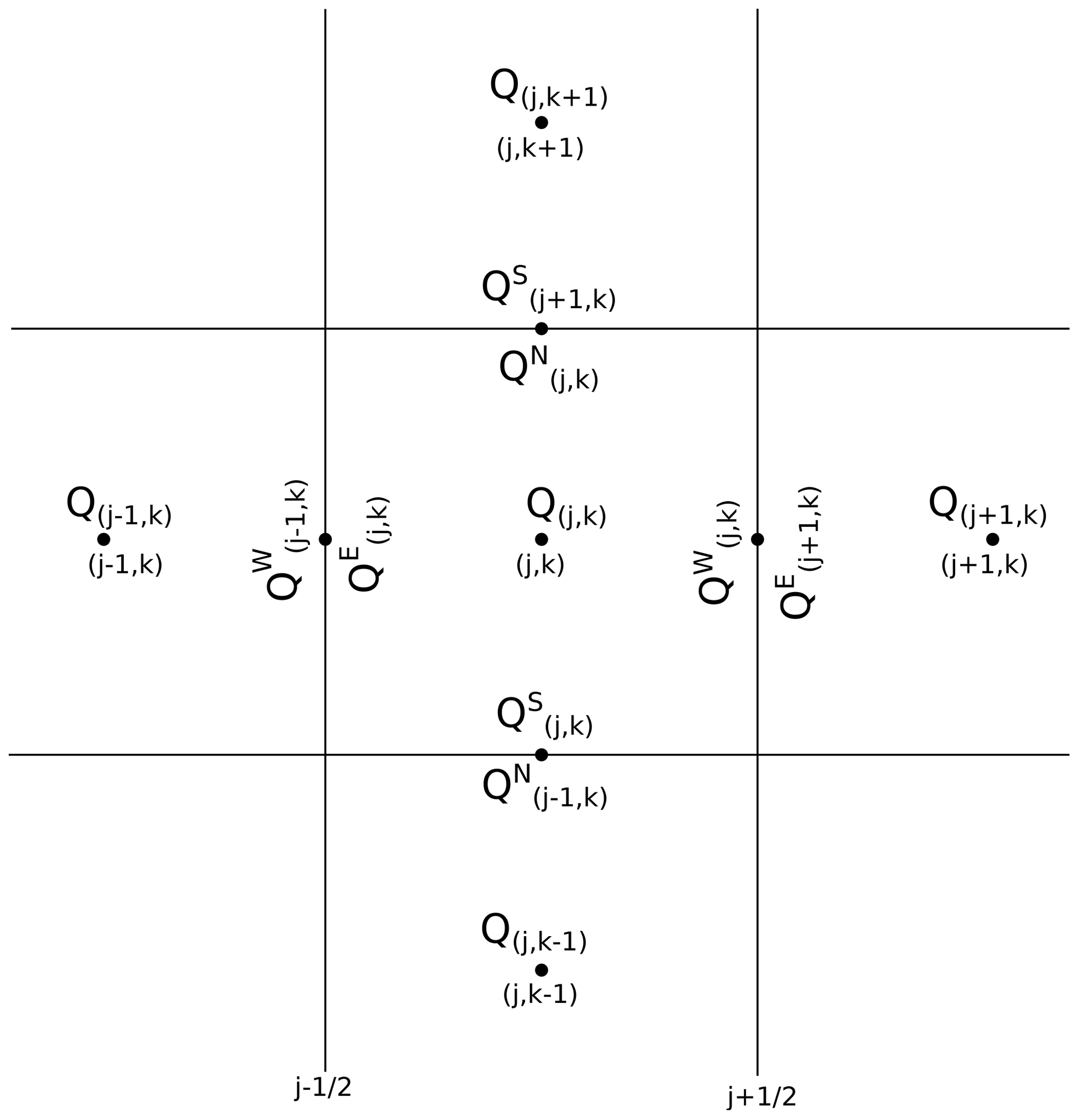
Figure 1 Sketch of the numerical grid and conservative variable indexing. The average value of the vector of conservative variables on each computational cell is denoted by Q_j,k and is associated with the cell centre. The vectors ${\mathbf{Q}}_{j,k}^{\mathrm{E}}$, ${\mathbf{Q}}_{j,k}^{\mathrm{W}}$, ${\mathbf{Q}}_{j,k}^{\mathrm{N}}$ and ${\mathbf{Q}}_{j,k}^{\mathrm{S}}$ are defined at the cell interfaces and represent the interface values of the conservative variables. At each interface two interface vectors are defined.

From the values of the primitive variables P_j,k at the cell centres, the partial derivatives (P_x)_j,k and (P_y)_j,k are computed, using opportune slope limiters (MinMod, Superbee or van Leer). Slope limiters are employed to mitigate the occurrence of excessive oscillations and unrealistic behaviour that might arise during the solution of partial differential equations through finite-volume methods, especially in proximity to shocks and discontinuities. When prioritizing accurate shock representation, the Superbee slope limiter can be the best choice as it maintains sharper discontinuities but at the cost of a tendency for smooth humps to become steeper and squared with time. If preserving monotonicity and minimizing oscillations in smooth regions are more important, then MinMod could be favoured. For a more detailed analysis of slope limiters and finite-volume methods, the reader can refer to LeVeque (2002). Once the partial derivatives are computed, the values at the internal sides of each cell interface are reconstructed with a linear interpolation from the cell centre values:

$$\begin{array}{l}{\displaystyle }{\mathbf{P}}_{j,k}^{\mathrm{E}}={\mathbf{P}}_{j,k}+{\displaystyle \frac{\mathrm{\Delta }x}{\mathrm{2}}}({\mathbf{P}}_x{)}_{j,k},{\mathbf{P}}_{j,k}^{\mathrm{W}}={\mathbf{P}}_{j,k}-{\displaystyle \frac{\mathrm{\Delta }x}{\mathrm{2}}}({\mathbf{P}}_x{)}_{j,k},\\ {\displaystyle }{\mathbf{P}}_{j,k}^{\mathrm{N}}={\mathbf{P}}_{j,k}+{\displaystyle \frac{\mathrm{\Delta }y}{\mathrm{2}}}({\mathbf{P}}_y{)}_{j,k},{\mathbf{P}}_{j,k}^{\mathrm{S}}={\mathbf{P}}_{j,k}-{\displaystyle \frac{\mathrm{\Delta }y}{\mathrm{2}}}({\mathbf{P}}_y{)}_{j,k}.\end{array}$$

This choice for primitive variables allows prescription of the boundary conditions at the cell interfaces in a natural way because usually they are given in terms of flow thickness, volumetric flow rate, phase fractions and temperature or in terms of their gradient. Having two different values at the two sides of interfaces in a numerical method might seem counterintuitive from a physical standpoint. However, these jumps are a consequence of the mathematical discretization process used in the finite-volume method to approximate continuous partial differential equations over discrete domains. In particular, having two values at the two sides of interfaces in finite-volume methods is essential for properly describing and capturing discontinuous solutions (LeVeque, 2002).

Once the primitive variables at the interfaces are known (either from the reconstruction or from the boundary conditions at the boundary cells), we compute the corresponding conservative variables ${\mathbf{Q}}_{j,k}^{\mathrm{E}}$, ${\mathbf{Q}}_{j,k}^{\mathrm{W}}$, ${\mathbf{Q}}_{j,k}^{\mathrm{N}}$ and ${\mathbf{Q}}_{j,k}^{\mathrm{S}}$. Primitive and conservative variables are then used to compute the fluxes $\mathbf{F}({\mathbf{P}}_{j,k}^{(\cdot )},{\mathbf{Q}}_{j,k}^{(\cdot )})$ and $\mathbf{G}({\mathbf{P}}_{j,k}^{(\cdot )},{\mathbf{Q}}_{j,k}^{(\cdot )})$ at the sides of the interfaces. We observe that the set of primitive variables is redundant, but this redundancy allows us to obtain a stable numerical scheme. In particular, for the advective flux terms, the advection velocity components are obtained from the primitive variables, while the variables to advect are taken directly from the conservative variables. The use of this combination of reconstructed primitive and conservative variables for the calculation of the fluxes, together with the application of limiters, makes the numerical scheme stable, avoiding the origin of large values of thickness and velocity. The fluxes at the two sides of each interface are then used to compute the numerical fluxes.

Following Kurganov and Petrova (2007), the numerical fluxes in the x direction are given by

$$\begin{array}{ll}{\displaystyle }{\mathbf{H}}_{j+\frac{\mathrm{1}}{\mathrm{2}},k}^x=& {\displaystyle \frac{a_{j+\frac{\mathrm{1}}{\mathrm{2}},k}^{+}\mathbf{F}({\mathbf{P}}_{j,k}^{\mathrm{E}},{\mathbf{Q}}_{j,k}^{\mathrm{E}})-a_{j+\frac{\mathrm{1}}{\mathrm{2}},k}^{-}\mathbf{F}({\mathbf{P}}_{j+\mathrm{1},k}^{\mathrm{W}},{\mathbf{Q}}_{j+\mathrm{1},k}^{\mathrm{W}})}{a_{j+\frac{\mathrm{1}}{\mathrm{2}},k}^{+}-a_{j+\frac{\mathrm{1}}{\mathrm{2}},k}^{-}}}\\ \text{(25)}& {\displaystyle }& {\displaystyle }+{\displaystyle \frac{a_{j+\frac{\mathrm{1}}{\mathrm{2}},k}^{+}{a}_{j+\frac{\mathrm{1}}{\mathrm{2}},k}^{-}}{a_{j+\frac{\mathrm{1}}{\mathrm{2}},k}^{+}-a_{j+\frac{\mathrm{1}}{\mathrm{2}},k}^{-}}}\left({\mathbf{Q}}_{j+\mathrm{1},k}^{\mathrm{W}}-{\mathbf{Q}}_{j,k}^{\mathrm{E}}\right),\end{array}$$

where the right- and left-going local speeds $a_{j+\frac{\mathrm{1}}{\mathrm{2}},k}^{+}$ and $a_{j+\frac{\mathrm{1}}{\mathrm{2}},k}^{-}$ are estimated by

$$\begin{array}{c}{\displaystyle }{a}_{j+\frac{\mathrm{1}}{\mathrm{2}},k}^{+}=max(u_{j,k}^{\mathrm{E}}+\sqrt{g^{\prime }{h}_{j,k}^{\mathrm{E}}},u_{j+\mathrm{1},k}^{\mathrm{W}}+\sqrt{g^{\prime }{h}_{j+\mathrm{1},k}^{\mathrm{W}}},\mathrm{0}),\\ {\displaystyle }{a}_{j+\frac{\mathrm{1}}{\mathrm{2}},k}^{-}=min(u_{j,k}^{\mathrm{E}}-\sqrt{g^{\prime }{h}_{j,k}^{\mathrm{E}}},u_{j+\mathrm{1},k}^{\mathrm{W}}-\sqrt{g^{\prime }{h}_{j+\mathrm{1},k}^{\mathrm{W}}},\mathrm{0}).\end{array}$$

It is important here to remark that we have two local speeds not because they are associated with the two different sides of each interface but because one is for the left-going characteristic speeds (on both sides) and the other for the right-going speeds (on both sides).

In a similar way, the numerical fluxes in the y direction are given by

$$\begin{array}{ll}{\displaystyle }{\mathbf{H}}_{j,k+\frac{\mathrm{1}}{\mathrm{2}}}^y=& {\displaystyle \frac{b_{j,k+\frac{\mathrm{1}}{\mathrm{2}}}^{+}\mathbf{G}({\mathbf{P}}_{j,k}^{\mathrm{N}},{\mathbf{Q}}_{j,k}^{\mathrm{N}}))-b_{j,k+\frac{\mathrm{1}}{\mathrm{2}}}^{-}\mathbf{G}({\mathbf{P}}_{j+\mathrm{1},k}^{\mathrm{S}},{\mathbf{Q}}_{j+\mathrm{1},k}^{\mathrm{S}})}{b_{j,k+\frac{\mathrm{1}}{\mathrm{2}}}^{+}-b_{j,k+\frac{\mathrm{1}}{\mathrm{2}}}^{-}}}\\ \text{(26)}& {\displaystyle }& {\displaystyle }+{\displaystyle \frac{b_{j,k+\frac{\mathrm{1}}{\mathrm{2}}}^{+}{b}_{j,k+\frac{\mathrm{1}}{\mathrm{2}}}^{-}}{b_{j,k+\frac{\mathrm{1}}{\mathrm{2}}}^{+}-b_{j,k+\frac{\mathrm{1}}{\mathrm{2}}}^{-}}}\left({\mathbf{Q}}_{j+\mathrm{1},k}^{\mathrm{S}}-{\mathbf{Q}}_{j,k}^{\mathrm{N}}\right),\end{array}$$

where the local speeds in the y direction, $b_{j+\frac{\mathrm{1}}{\mathrm{2}},k}^{+}$ and $b_{j+\frac{\mathrm{1}}{\mathrm{2}},k}^{-}$, are given by

$$\begin{array}{c}{\displaystyle }{b}_{j,k+\frac{\mathrm{1}}{\mathrm{2}}}^{+}=max(v_{j,k}^{\mathrm{N}}+\sqrt{g^{\prime }{h}_{j,k}^{\mathrm{N}}},v_{j,k+\mathrm{1}}^{\mathrm{S}}+\sqrt{g^{\prime }{h}_{j,k+\mathrm{1}}^{\mathrm{S}}},\mathrm{0}),\\ {\displaystyle }{b}_{j,k+\frac{\mathrm{1}}{\mathrm{2}}}^{-}=min(v_{j,k}^{\mathrm{N}}-\sqrt{g^{\prime }{h}_{j,k}^{\mathrm{N}}},v_{j,k+\mathrm{1}}^{\mathrm{S}}-\sqrt{g^{\prime }{h}_{j,k+\mathrm{1}}^{\mathrm{S}}},\mathrm{0}).\end{array}$$

The explicit computation of the term S₁ requires the numerical discretization of the spatial gradient of the topography. The partial derivatives (B_x)_j,k and (B_y)_j,k are computed from the cell averages using the same slope limiter that is used for h. Then, the topography is computed at the interfaces with a linear reconstruction, obtaining the values for each cell:

$$\begin{array}{l}{\displaystyle }{\mathbf{B}}_{j,k}^{\mathrm{E}}={\mathbf{B}}_{j,k}+{\displaystyle \frac{\mathrm{\Delta }x}{\mathrm{2}}}({\mathbf{B}}_x{)}_{j,k},{\mathbf{B}}_{j,k}^{\mathrm{W}}={\mathbf{B}}_{j,k}-{\displaystyle \frac{\mathrm{\Delta }x}{\mathrm{2}}}({\mathbf{B}}_x{)}_{j,k},\\ {\displaystyle }{\mathbf{B}}_{j,k}^{\mathrm{N}}={\mathbf{B}}_{j,k}+{\displaystyle \frac{\mathrm{\Delta }y}{\mathrm{2}}}({\mathbf{B}}_y{)}_{j,k},{\mathbf{B}}_{j,k}^{\mathrm{S}}={\mathbf{B}}_{j,k}-{\displaystyle \frac{\mathrm{\Delta }y}{\mathrm{2}}}({\mathbf{B}}_y{)}_{j,k}.\end{array}$$

The implicit part of the IMEX Runge–Kutta scheme, associated with the integration of the friction terms, is solved using a Newton–Raphson method with an optimum step size control, where the Jacobian of the implicit terms is computed with an automatic complex-step derivative approximation (de' Michieli Vitturi et al., 2019). The implicit treatment of the friction terms, when dealing with strongly non-linear rheologies, avoids many problems related to the proper stopping condition of the flow without the need to introduce arbitrary thresholds. In addition, the automatic derivation of the friction term allows for a simple implementation of additional rheological models, including formulations dependent on any model parameter.

After each Runge–Kutta procedure, the sedimentation and air entrainment term are computed explicitly and the flow variables and the topography at the centres of the computational cells are updated.

For large time steps, the explicit treatment of solid sedimentation could lead to negative solid volumetric fractions in the flow, and for this reason the effective sedimentation rate ${\stackrel{\mathrm{‾}}{S}}_{\mathrm{s},i_{\mathrm{s}}}$ is limited at each integration step in order to prevent this occurrence:

$${\stackrel{\mathrm{‾}}{S}}_{\mathrm{s},i_{\mathrm{s}}}=min\left[S_{\mathrm{s},i_{\mathrm{s}}},\mathrm{\Delta }t\cdot \left({\mathit{\alpha }}_{\mathrm{s},i_{\mathrm{s}}}h\right)\right].$$

The use of an explicit integration scheme for the terms of the equations containing spatial derivatives, with respect to an implicit treatment, has the advantage that the solutions of the discretized equations in each cell are decoupled without the need to solve for a large linear system. The same is true for the integration of the friction, sedimentation and entrainment terms. This allowed implementation of a parallel strategy to advance in time the numerical solution of the discretized equations, requiring almost no communication or dependency between the processes. Thus, with a small effort, the Fortran implementation of the code has been updated by parallelizing all the loops over the computational cells with the Open Multi-Processing (OpenMP) programming model for shared-memory platforms.

The schemes implemented for the numerical discretization of the governing equations do not depend on the particular choice of the constitutive equation or on the friction force; thus they apply also when the model is used to solve for different volcanic mass flows.

5  Numerical benchmarks

In this section we present applications of the model to 1D and 2D problems. They provide some of the fundamental elements for verification and validation of the numerical model (following the terminology proposed by Oberkampf and Trucano, 2002, and Esposti Ongaro et al., 2020), adding to numerical benchmarks and validation tests previously presented by de' Michieli Vitturi et al. (2019). The 1D benchmark tests are designed to demonstrate the capability of the numerical scheme to describe the interaction of the flow with obstacles in different regimes (subcritical, supercritical, transitional). Then, model results are compared with those presented in Engwell et al. (2016) for large ash flows to compare the steady state produced by our 2D transient simulations with that obtained with a 1D axisymmetric steady-state model.

5.1 One-dimensional subcritical and transcritical flows

When dealing with flows where velocity and mixture density can experience large changes, it is important to have a model which properly describes both subcritical (Ri>1) and supercritical (Ri<1) regimes and the transition between them. In the subcritical regime, flow is dominated by gravitational forces, with greater thickness and lower velocities; for supercritical flow it is the opposite, with thinner and faster flow dominated by inertial forces. In addition, it is fundamental to have a model that is able to describe accurately how the flow interacts with the topography under these different regimes. As shown in Woods et al. (1998) using both laboratory experiments and theoretical models, when a flow interacts with a topographic barrier such as a ridge, the flow thickness and velocity can change in different ways depending on the height of the ridge and the flow speed (Houghton and Kasahara, 1968). Under some circumstances, flows may be partially blocked and produce upstream-propagating bores resulting in increased sedimentation upstream of the barrier. In other cases, the flow is able to overcome the ridge but with a transition in flow regime and thus in the sedimentation pattern.

Here, we present some numerical simulations reproducing literature benchmarks and showing the capability of the numerical code to properly model the subcritical and supercritical regimes and the transition between them. Following Goutal (1997), Delestre et al. (2013) and Michel-Dansac et al. (2016), we simulate a steady one-dimensional flow in a 25 m domain with a parabolic bump on the bottom, where the topography is given by

$$\begin{array}{}\text{(27)}& B\left(x\right)=\left\{\begin{array}{ll}\mathrm{0.2}-\mathrm{0.05}(x-\mathrm{10}{)}^{\mathrm{2}}& \text{when}\mathrm{8}<x<\mathrm{12},\\ \mathrm{0}& \text{elsewhere}.\end{array}\right.\end{array}$$

For the test cases presented in this section, no friction, mass entrainment and sedimentation are considered. The flow travels in the x direction (u>0 m s⁻¹, v=0 m s⁻¹), with constant density (for simplicity ρ=1 kg m⁻³) and constant temperature (energy equation is not needed). With these assumptions, in the steady-state regime, we can derive from Eqs. (2)–(3) the following simpler governing equations:

$$\begin{array}{}\text{(28)}& \left\{\begin{array}{l}\frac{\partial \left(hu\right)}{\partial x}=\mathrm{0},\\ \\ \frac{\partial }{\partial x}\left(h{u}^{\mathrm{2}}+\frac{\mathrm{1}}{\mathrm{2}}{g}^{\prime }{h}^{\mathrm{2}}\right)=-g^{\prime }h\frac{\partial B}{\partial x}.\end{array}\right.\end{array}$$

By expanding the derivative on the left-hand side of the momentum equation, we obtain

$$\begin{array}{}\text{(29)}& u{\displaystyle \frac{\partial u}{\partial x}}+g^{\prime }{\displaystyle \frac{\partial h}{\partial x}}=-g^{\prime }{\displaystyle \frac{\partial B}{\partial x}},\end{array}$$

and, by substituting the expression of $\partial u/\partial x$ computed from the mass equation, we have

$$\begin{array}{}\text{(30)}& \left(\mathrm{1}-{\displaystyle \frac{u^{\mathrm{2}}}{g^{\prime }h}}\right){\displaystyle \frac{\partial h}{\partial x}}=-{\displaystyle \frac{\partial B}{\partial x}},\end{array}$$

which, written in terms of the Richardson number Ri, gives

$$\begin{array}{}\text{(31)}& \begin{array}{rl}& \left(\mathrm{1}-{\displaystyle \frac{\mathrm{1}}{Ri}}\right){\displaystyle \frac{\partial h}{\partial x}}=-{\displaystyle \frac{\partial B}{\partial x}}\\ & \text{or}\left(\mathrm{1}-Ri\right){\displaystyle \frac{\partial }{\partial x}}(h+B)={\displaystyle \frac{\partial B}{\partial x}}.\end{array}\end{array}$$

According to these equations, the subcritical or supercritical regime determines whether flow thickness h and free surface h+B increase or decrease as the fluid interacts with the topography. It is also important to observe that in supercritical flows (Ri<1), upstream conditions fully determine the flow immediately downstream, while in subcritical flows changes in downstream conditions affect the flow upstream. From a numerical point of view, this is important when prescribing flow boundary conditions because we can only prescribe all flow variables at the inlet for supercritical flows. We remark here that the test cases presented in this section are not meant to be representative of real dilute PDC conditions, but they have been chosen to show the capability of the numerical model to properly simulate different flow regimes and their transitions.

By integrating Eq. (30) with the additional condition of constant volumetric flux, as expressed by the first part of Eq. (28), we also have, in the case of a regular solution, the following Bernoulli equation:

$$\begin{array}{}\text{(32)}& {\displaystyle \frac{(hu{)}^{\mathrm{2}}}{\mathrm{2}{g}^{\prime }{h}^{\mathrm{2}}}}+h+z=\mathrm{Const},\end{array}$$

which gives a relation between the topography elevation and the flow height. Using Eq. (32), in the cases of supercritical or subcritical flows without regime transitions, it is possible to obtain the following implicit equation for the flow depth (Delestre et al., 2013):

$$\begin{array}{}\text{(33)}& h(x{)}^{\mathrm{3}}+\left(B\left(x\right)-{\displaystyle \frac{(h_{\mathrm{0}}{u}_{\mathrm{0}}{)}^{\mathrm{2}}}{\mathrm{2}{g}^{\prime }{h}_{\mathrm{0}}^{\mathrm{2}}}}\right)h(x{)}^{\mathrm{2}}+{\displaystyle \frac{(h_{\mathrm{0}}{u}_{\mathrm{0}}{)}^{\mathrm{2}}}{\mathrm{2}{g}^{\prime }}}=\mathrm{0},\end{array}$$

where h₀ and u₀ are the flow thickness and velocity at the inlet and outlet of the domain, respectively.

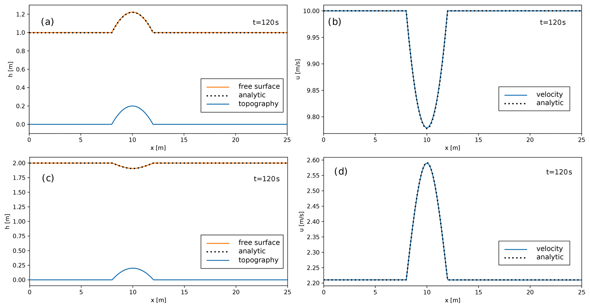
Figure 2 Thickness (a, c) and velocity (b, d) profiles in one-dimensional flows over a bump. Steady-state numerical solutions for supercritical and subcritical flows are shown with solid lines in the top and bottom panels, respectively. The dotted black lines in each panel represent the analytical solutions, computed by solving Eq. (33).

The first test case is a flow where at the left boundary of the domain an influx with h=1 m and u=10 m s⁻¹ is prescribed, resulting in a supercritical regime ($Ri<{\mathrm{10}}^{-\mathrm{2}}$). As previously stated, the supercritical conditions at the inlet are consistent with the two boundary conditions assigned. For this simulation, as for the other simulations presented in this section, the domain is partitioned with 1000 uniform cells, and a linear reconstruction of the primitive variables with a MinMod limiter has been used. For this supercritical test, the solution at t=0 is initialized with a constant thickness corresponding to the inlet value and with zero velocity. The solution at t=120 s, when a steady state is reached, is presented in terms of the flow free surface (Fig. 2a, orange line) and flow velocity (Fig. 2b). In this supercritical condition, the fluid thickens and slows as it passes over the top of the obstacle, reaching its minimum speed at the crest (x=10 m). The slope of the free surface follows the slope of the obstacle, increasing before the crest and then decreasing in elevation. The higher the Richardson number, the smaller the effect of topography on flow thickness and on velocity, with the free surface mimicking the slope of the topography.

The second test case is a simulation of a subcritical regime. In this case an influx of 4.42 m² s⁻¹ is prescribed at the left boundary, while a flow thickness of 2 m is fixed at the outlet. It is important to observe that here, in contrast to the previous case, we cannot prescribe both flow thickness and velocity at the inlet because of the subcritical condition. Also for this case, the solution in the domain is initialized at t=0 s with a constant thickness corresponding to the outlet value and with zero velocity. The numerical solution at t=120 s, corresponding to a steady state, is presented in the bottom panels of Fig. 2. In this case, the fluid thins and accelerates as it crosses the top of the obstacle, reaching its maximum speed and minimum thickness at the crest. Accordingly with the second part of Eq. (31), the free surface also decreases where the bottom slope is positive, while it increases after reaching the bottom crest. For both the first two test cases, we also computed the analytical solutions by means of the Bernoulli equation (Eq. 33), and the values are plotted with dotted black lines in Fig. 2, showing a good correspondence with the numerical solutions (solid lines).

The interaction of a flow with an obstacle can also lead to a steady solution, with a transition in the flow regime (transcritical flow). The steady-state conditions investigated here for these transonic (with and without shock) test cases are similar to those obtained in laboratory experiments presented in Fig. 4a of Woods et al. (1998), which showed that the deposit is weakly affected by the presence of the ridge and the regime transition. If the flow is subcritical upstream and it undergoes a sufficient increase in velocity and decrease in thickness as it ascends towards the crest, a smooth transition from subcritical to supercritical flow can occur. This transition is shown in the top panels of Fig. 3, representing the flow free surface at t=120 s for a flow with an influx of 1.53 m² s⁻¹ prescribed at the left boundary and a thickness of 0.66 m fixed at the outlet, when the flow is subcritical. In fact, when the flow becomes supercritical, no boundary condition can be prescribed at the outlet, and the outlet thickness is an outcome of the simulation (here h=0.4 m). For this simulation, the solution in the domain is initialized at t=0 s with a constant free surface corresponding to the outlet subcritical value and with zero velocity. Also in the case of transcritical flow without shock, it is possible to express, from the Bernoulli equation (Eq. 32), the water height as the solution of a cubic equation (Delestre et al., 2013):

$$\begin{array}{}\text{(34)}& \begin{array}{rl}& h(x{)}^{\mathrm{3}}+\left(B\left(x\right)-{\displaystyle \frac{(h_{\mathrm{0}}{u}_{\mathrm{0}}{)}^{\mathrm{2}}}{\mathrm{2}{g}^{\prime }{h}_{\mathrm{C}}^{\mathrm{2}}}}-h_{\mathrm{C}}-B_{\mathrm{M}}\right)h(x{)}^{\mathrm{2}}\\ & +{\displaystyle \frac{(h_{\mathrm{0}}{u}_{\mathrm{0}}{)}^{\mathrm{2}}}{\mathrm{2}{g}^{\prime }}}=\mathrm{0},\end{array}\end{array}$$

where h₀ and u₀ are the flow thickness and velocity at the inlet or outlet of the domain, respectively; B_M is the maximum topography elevation; and h_C is the corresponding flow thickness, which can be computed analytically as (Delestre, 2010)

$$h_{\mathrm{C}}={\left({\displaystyle \frac{h_{\mathrm{0}}{u}_{\mathrm{0}}}{\sqrt{g^{\prime }}}}\right)}^{\mathrm{2}/\mathrm{3}}.$$

The analytical solution of the Eq. (34) is reported in the top panels of Fig. 3 with a dotted black line.

Under certain conditions, the flow, after an initial thinning and acceleration over the obstacle, can suddenly thicken and decelerate with a shock in correspondence to a flow regime transition. This transition from a rapid, supercritical flow to a slow, subcritical flow, called a hydraulic jump, is shown in Fig. 3, bottom panels, representing the flow free surface at t=120 s for a flow with an influx of 0.18 m² s⁻¹ prescribed at the left boundary and a thickness of 0.33 m fixed at the outlet. Following Delestre et al. (2013), flow thickness for the transcritical flow with shock is given by the solution of

$$\begin{array}{}\text{(35)}& \left\{\begin{array}{ll}& h(x{)}^{\mathrm{3}}+\left(B\left(x\right)-\frac{(h_{\mathrm{0}}{u}_{\mathrm{0}}{)}^{\mathrm{2}}}{\mathrm{2}{g}^{\prime }{h}_{\mathrm{C}}^{\mathrm{2}}}-h_{\mathrm{C}}-B_{\mathrm{M}}\right)h(x{)}^{\mathrm{2}}+\frac{(h_{\mathrm{0}}{u}_{\mathrm{0}}{)}^{\mathrm{2}}}{\mathrm{2}{g}^{\prime }}=\mathrm{0},\\ & x<x_{\mathrm{shock}};\\ & h(x{)}^{\mathrm{3}}+\left(B\left(x\right)-\frac{(h_{\mathrm{0}}{u}_{\mathrm{0}}{)}^{\mathrm{2}}}{\mathrm{2}{g}^{\prime }{h}_{\mathrm{0}}^{\mathrm{2}}}\right)h(x{)}^{\mathrm{2}}+\frac{(h_{\mathrm{0}}{u}_{\mathrm{0}}{)}^{\mathrm{2}}}{\mathrm{2}{g}^{\prime }}=\mathrm{0},\\ & x>x_{\mathrm{shock}};\\ & \left(h\right(x\left)u\right(z){)}^{\mathrm{2}}\left(\frac{\mathrm{1}}{h_{\mathrm{1}}}-\frac{\mathrm{1}}{h_{\mathrm{2}}}\right)+\frac{g^{\prime }}{\mathrm{2}}(h_{\mathrm{1}}^{\mathrm{2}}-h_{\mathrm{2}}^{\mathrm{2}})=\mathrm{0},\end{array}\right.\end{array}$$

where B_M is the maximum topography elevation; h₀ and u₀ are the flow thickness and velocity at the outlet of the domain, respectively; h_C is the corresponding flow thickness; and h₁ and h₂ are the flow thicknesses upstream and downstream of the shock, respectively. The location of the shock x_shock is found from the last part of Eq. (35), which is the Rankine–Hugoniot’s condition (LeVeque, 2002). The analytical solution of Eq. (35) is plotted in the bottom panels of Fig. 3 with a dotted black line, showing the accuracy of the numerical solver in the prediction of the shock location and amplitude for both flow thickness and velocity.

Figure 3 Flow thickness (a, c) and velocity (b, d) profiles in one-dimensional flows over a bump. Steady numerical solutions for transcritical flows without and with shock are shown with solid lines in the top and bottom panels, respectively. The dotted black lines in each panel represent the analytical solutions, computed by solving Eqs. (34) and (35).

In addition to the literature test cases described above, aimed at reproducing steady-state flows for different regimes, we present here another test case showing the temporal evolution of a flow with a steady inlet condition, where the interaction with an obstacle results in the transition from a subcritical to supercritical regime and the backward propagation of a hydraulic jump. The boundary conditions (inlet and outlet) are based on the configurations described in Khezri (2014) and Putra et al. (2019), and, as for the previous tests, we assume a constant density (ρ=1 kg m⁻³) and neglect friction, mass entrainment and sedimentation. The computational domain is 10 m long (discretized with 1000 cells), and the inlet flow velocity and thickness are fixed to 0.74 m s⁻¹ and 0.14 m, respectively. The same values are used for the initial conditions up to 8 m from the inlet, while no flow is present beyond this distance. At a distance of 9 m from the inlet, a 0.1 m high wall is present, represented by a discontinuity in the topography:

$$\begin{array}{}\text{(36)}& B\left(x\right)=\left\{\begin{array}{ll}\mathrm{0},& x\le \mathrm{9}\mathrm{m};\\ \mathrm{0.1},& x>\mathrm{9}\mathrm{m}.\end{array}\right.\end{array}$$

For this test case, no analytical solutions are available. Some snapshots of the first 40 s of the simulation are shown in Fig. 4, with the flow thickness in the left panels and the velocity in the right panels. When the flow front reaches the wall, flow thickness increases and its velocity decreases, with a transition from a supercritical to subcritical regime. The transition zone propagates backward, similarly to a tidal bore. At the same time, due to an increase in flow thickness, part of the flow overcomes the obstacle and propagates beyond it. This behaviour is similar to that illustrated in Woods et al. (1998), their Fig. 9, for a large ash flow interacting with a ridge. While they interpreted the bore as a reflected part of the flow, which can carry fine-grained material back upstream, the right panels of Fig. 4 show that flow velocity is always positive. This means that, for the simulation presented here, the increase in flow thickness propagating upstream is due not to a negative flow velocity or a flow reflection but to the backward propagation of the hydraulic jump. At later stages (not shown here) a steady state is reached, with the flow being subcritical before and supercritical after the wall. A similar behaviour can be expected when a supercritical PDC reaches a sufficiently high topographic obstacle. This, because of the transition to a subcritical regime, would result in an increased sedimentation rate before the obstacle.

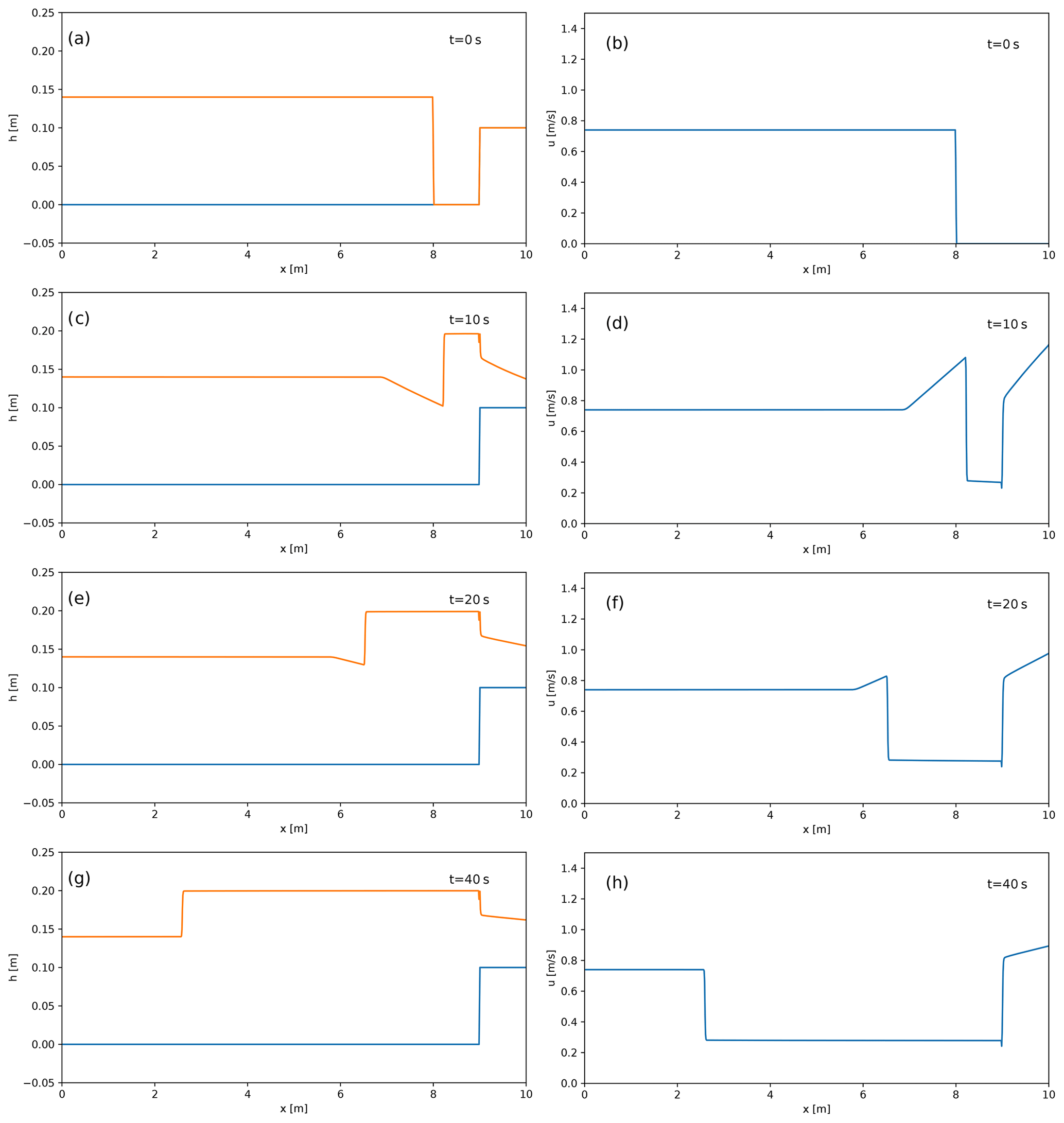
Figure 4 Thickness (left) and velocity (right) profiles for a one-dimensional subcritical flow with a backward-propagating hydraulic jump.

5.2 Radial ash flow

In this section we apply the new model to reproduce results presented in Engwell et al. (2016) for large dilute flows producing coignimbrite columns. Thus, in comparison to the test cases of the previous section, we model a mixture of gas and solid particles, here with a diameter of 100 µm. Solid sedimentation and atmospheric air entrainment are also modelled, resulting in a mixture for which temperature and density change during the transport. Engwell et al. (2016) used a steady-state 1D model with radial symmetry, and here we want to reproduce the steady condition with transient 2D simulations. To be consistent with the assumptions of Engwell et al. (2016) and to obtain a steady state, we do not consider any modification of the topography associated with the sedimentation of solid particles. In this way, with a steady source, it is possible to reach a steady condition and a steady radial profile. The use of a steady-state numerical code, as in Engwell et al. (2016), restricts the study to supercritical flows, and in this section we present numerical simulations for supercritical conditions only. As discussed for the previous example, subcritical and supercritical boundary conditions correspond to two different physical settings, and different boundary/source conditions are prescribed to model the different initial regimes. In the supercritical regime, flow downstream of the source is controlled by conditions upstream, and all the conservative variables must be fixed at the boundary inlet. This is the case for the two axisymmetric simulations presented in Figs. 5 and 6, where the initial Richardson numbers are 0.1 and 0.9, respectively. For both simulations the inlet conditions are given at R=2 km, with the initial thickness fixed at h=2 km, the initial gas mass fraction at 0.2, the initial temperature at T=900 K and the friction coefficient at 0.001. The initial velocities are computed from the other variables and the Richardson number, resulting in an initial radial velocity of 93.32 m s⁻¹ for Ri=0.9 and 279.98 m s⁻¹ for Ri=0.1. A 20 km by 20 km computational domain, discretized with 100 m size cells, is used for the two simulations. For both simulations, when the mixture becomes buoyant in a computational cell (due to entrainment and heating of atmospheric air and particle sedimentation), the mass is removed from that cell, while the solution is not computed for the cells that are fully inside the area defined by R<2 km. The two figures show the flow solution at t=200 s, when a steady condition for both radial flows is reached. In the left panels a 3D view of the flow thickness is presented. The colour of the free surface represents flow thickness, clearly showing a lower thickness for the simulation with initial Ri=0.9. When using Cartesian grids to model axisymmetric flows, it is not obvious that the output of the simulation would produce the correct results in terms of radial symmetry of the flow front. In fact, while the inlet velocity is given analytically at the lateral surface of the inlet cylinder, i.e. at a distance of 2 km from the point (0,0), the boundary conditions are prescribed numerically at the faces of the computational cells, which can be at different distances. For this reason, a correction of the velocity accounting for this discrepancy is applied to each inlet face. Model results, as shown in the left panels, highlight that this correction, coupled with the second-order discretization in space implemented in the model, correctly produces axisymmetric flows.

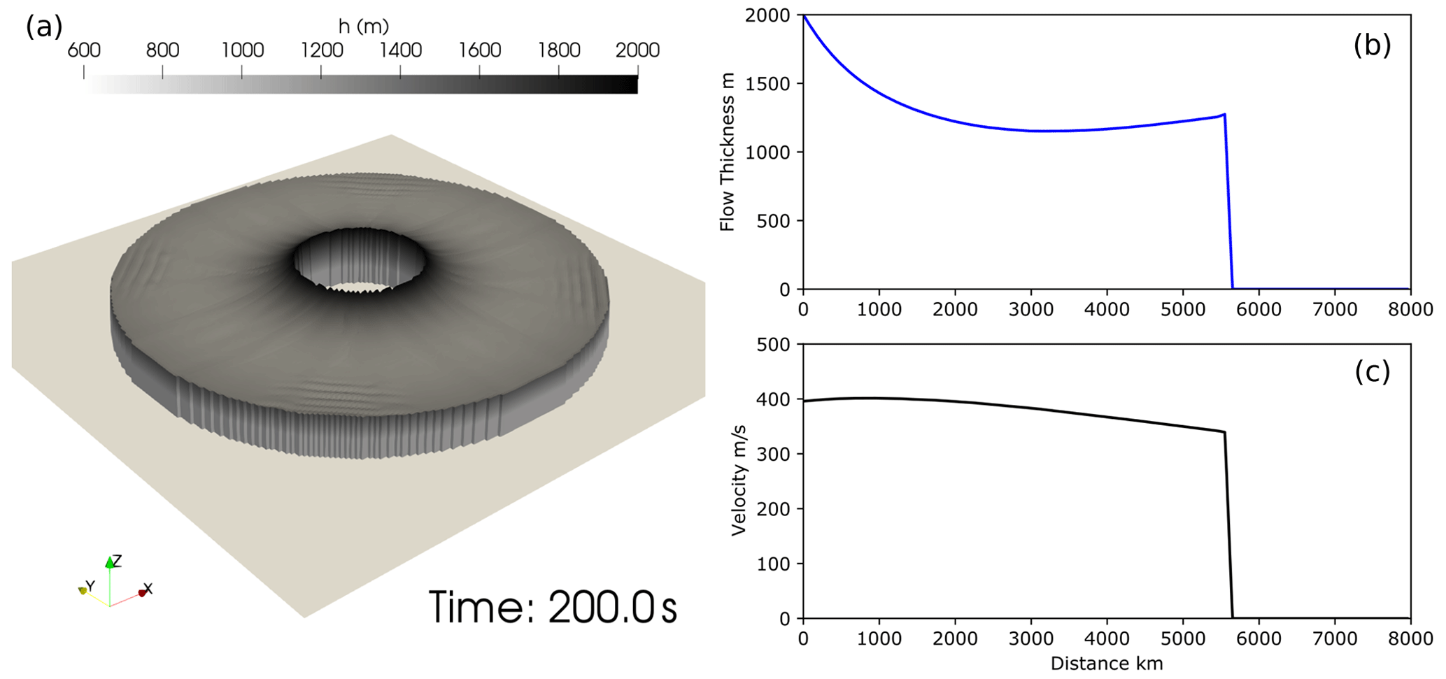
Figure 5 Supercritical flow with initial Ri=0.1. The solution is computed only for the cells of the computational domain outside (fully or partially) R=2000 m. The colour of the free surface represents flow thickness.

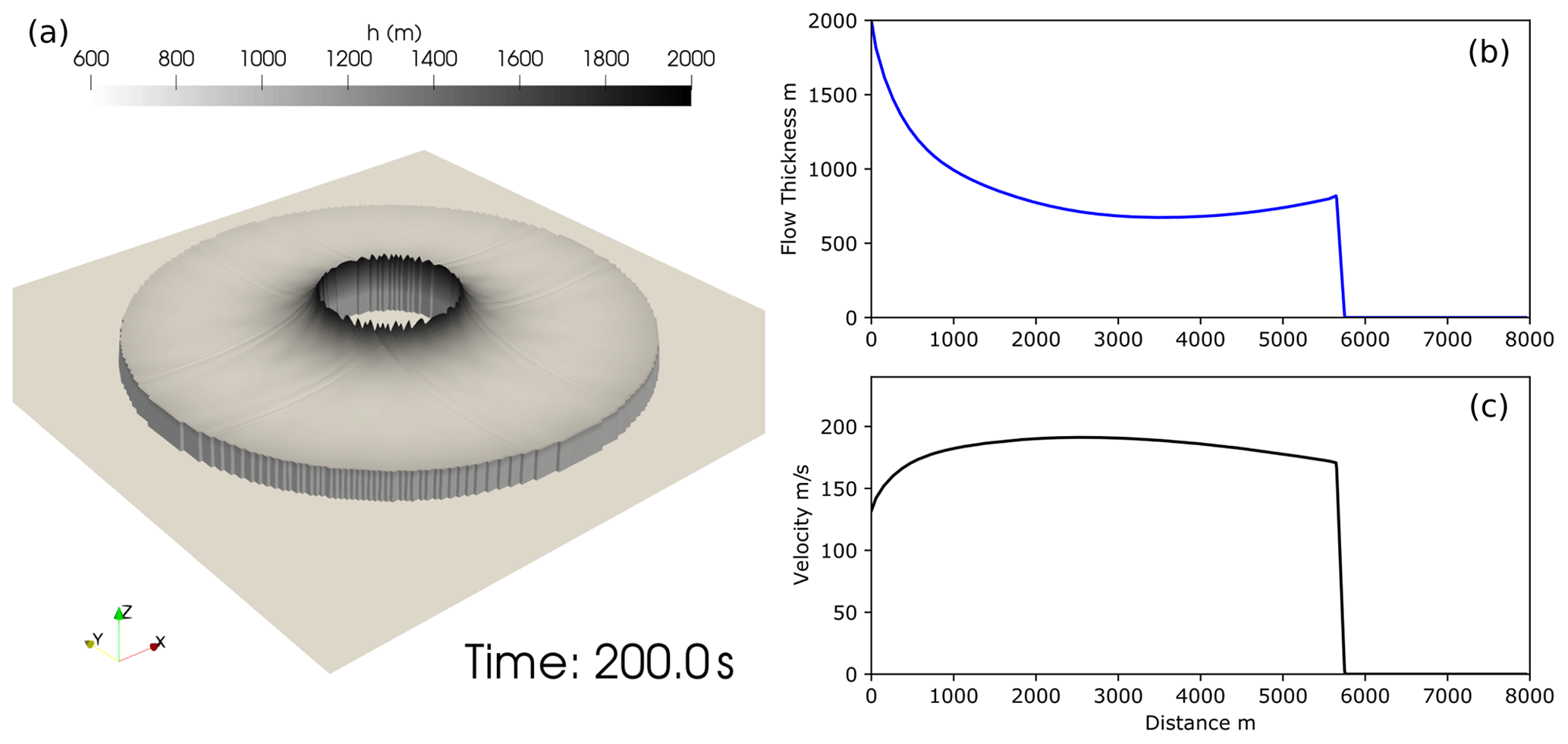
Figure 6 Supercritical flow with initial Ri=0.9. The solution is computed only for the cells of the computational domain outside (fully or partially) R=2000 m. The colour of the free surface represents flow thickness.

Plots of thickness and velocity along a radial section are shown in the right panels of Figs. 5 and 6, for the initial Richardson numbers of 0.1 and 0.9, respectively. These results can be compared with those presented in Engwell et al. (2016), their Fig. 3, where the same initial parameters have been used. For both initial conditions, model solutions show a decrease in flow thickness immediately after the source which is more pronounced for the largest value of Ri. Then, after approximately 3.5 km from the source, thickness increases again. These two different trends are due to the superposition of the thinning associated with the radial spreading and the thickening associated with atmospheric air entrainment, the first being more important close to the source and the second at greater distances (see also Calabrò et al., 2022). The velocity profiles of the two simulations present larger differences in the absolute values than the thickness, mostly because of the initial velocities associated with the different Richardson numbers. At the maximum runout distances, which are comparable for the two simulations, this results in a residual momentum for the simulation with Ri=0.1 being almost twice that for the simulation with Ri=0.9, as shown also by Engwell et al. (2016).

An advantage of a transient model, with respect to a steady one, is that the simulation can provide information on the propagation of the flow and the time needed to reach the maximum runout. Figure 7 shows the runout (solid green line) and the area invaded by the flow (dashed blue line) versus time for the two simulations presented above. In both simulations, we observe an almost linear increase in the area invaded with time, up to the time at which the maximum runout is reached. For the simulation with initial Ri=0.1, and thus with a larger flow velocity, the maximum runout is reached at t=28 s, while for the simulation with initial Ri=0.9, it is reached at t=79 s. Furthermore, we remark that only a transient model can simulate the modifications of the topography associated with the sedimentation of solid particles because of the intrinsic transient nature of this process.

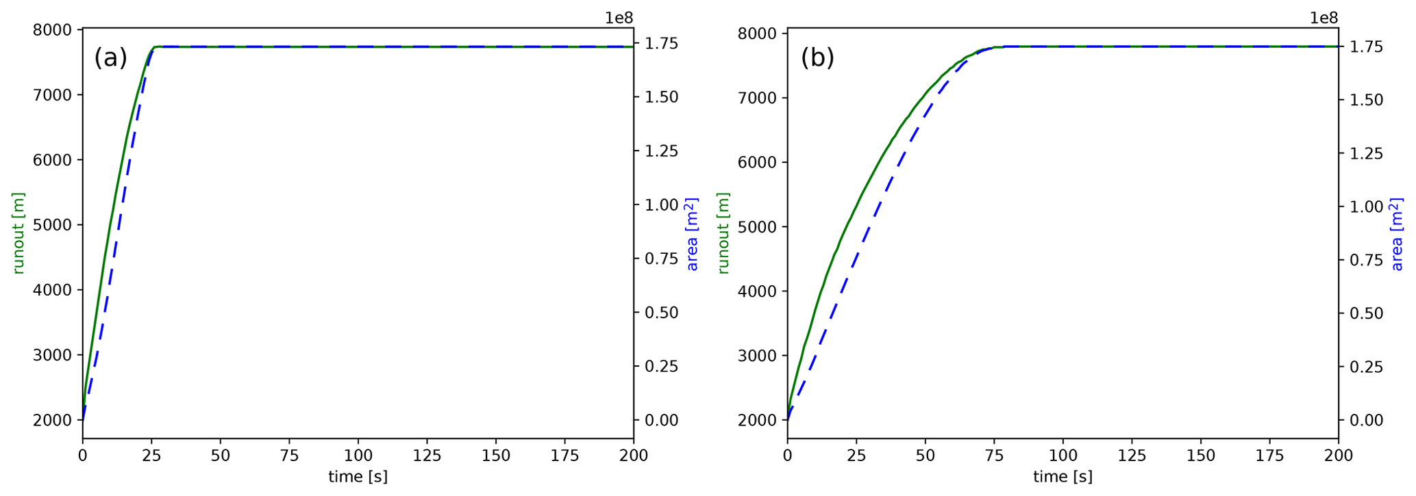
Figure 7 Runout (solid green line) and area invaded (dashed blue line) versus time for a simulation with initial Ri=0.1 (a) and Ri=0.9 (b).

6  PDCs over water: the Krakatau case study

Here we present an application of the model to Krakatau volcano, with inputs informed by the 1883 eruption. This simulation highlights the capability of the model to treat the interaction of the flow with topography, the presence of hydraulic jumps, and the vaporization and entrainment of water.

The Krakatau volcanic system is notorious for eruptive behaviour that interacts with the seas of the surrounding Sunda Strait. In 1883, an eruption produced PDCs that propagated more than 40 km across the sea (Carey et al., 1996), impacting populations on the coastlines of Sumatra and Java (Simpkin and Fiske, 1983) and potentially playing a role in the formation of devastating tsunamis that led to the deaths of > 36 000 people (Maeno and Imamura, 2011). Here, we test the flow model on real topography and investigate topographic effects on the flow regime and the transition from supercritical to subcritical flow. In addition, we show the effect of ingestion of seawater in the form of water vapour into the flows.

We test the flow over a water model formulation using the contemporary (i.e. representing recent topography rather than that in 1883) 30 m SRTM Void Filled DEM (USGS EarthExplorer, downloaded July 2021) of the area around the Krakatau volcanic complex and the Sunda Strait (Fig. 8). We assume that all cells with an elevation of zero are water. Model inputs were informed using information from the 1883 eruption from the published record and from field analysis of eruption deposits. An initial flow temperature of 773 K (500 ^∘C) was used based on results from Mandeville et al. (1994). However, the simulations are aimed not at replicating the eruption but at giving insight into the model application and the possible dynamics of these flows. We point out that we do not simulate here the collapse of the explosive column but only the dilute flow generated by the entrainment of atmospheric air and the collapse of the column. Thus, the initial conditions of the simulation refer to the source conditions of the radially spreading dilute flow. An initial flow radius of 2 km, flow Richardson number of 0.7 and mass flow rate of 10¹⁰ kg s⁻¹ were used. The initial density is 40 kg m⁻³. Initial flow thickness (≈310 m) and radial velocities (≈65 m s⁻¹) were calculated from these parameters. A particle class of 100 µm was used, and the gamma coefficient (${\mathit{\gamma }}_{i_{\mathrm{s}},\mathrm{wv}}$) was set to 0.86. This value was not constrained by observations but selected from an ensemble of simulations to better highlight some features of the flow (large entrainment of water vapour, hydraulic jumps, transient dynamics). Flow parameters were analysed along a number of transects (Fig. 8), which have different topographic profiles relating to the islands around the volcano (Fig. 9). A probe location is used to show how flow properties at a given location change with time.

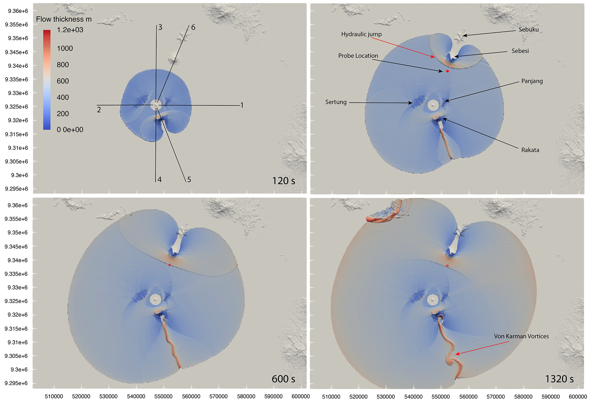
Figure 8 Snapshots of simulation SA4_0003, where a grain size of 100 µm, a mass flow rate of 10⁹ and a gamma coefficient (${\mathit{\gamma }}_{i_{\mathrm{s}},\mathrm{wv}}$) of 0.86 was used. Each image represents a different time step in the simulation. The red marker shows the probe location at 9338081 m N, 552669 m E (UTM Zone 48S). The topographic elevation for each transect is shown in Fig. 9.

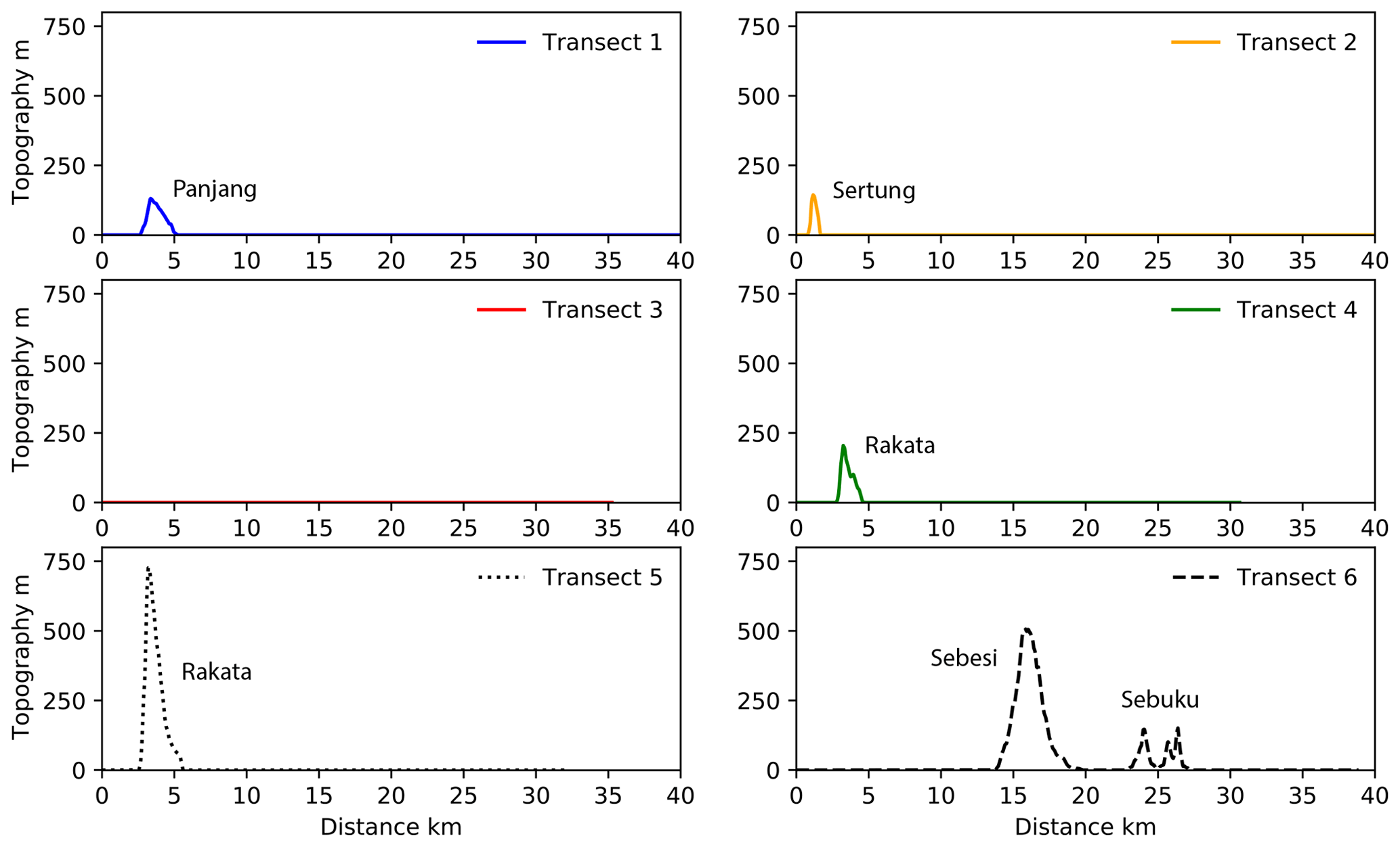
Figure 9 Topographic profiles of transects shown in Fig. 8a. Note the vertical exaggeration of the y axis. Transect 3 is the only transect that does not show variation in elevation along the flow runout; all other transects cross one of the many islands in the Sunda Strait.

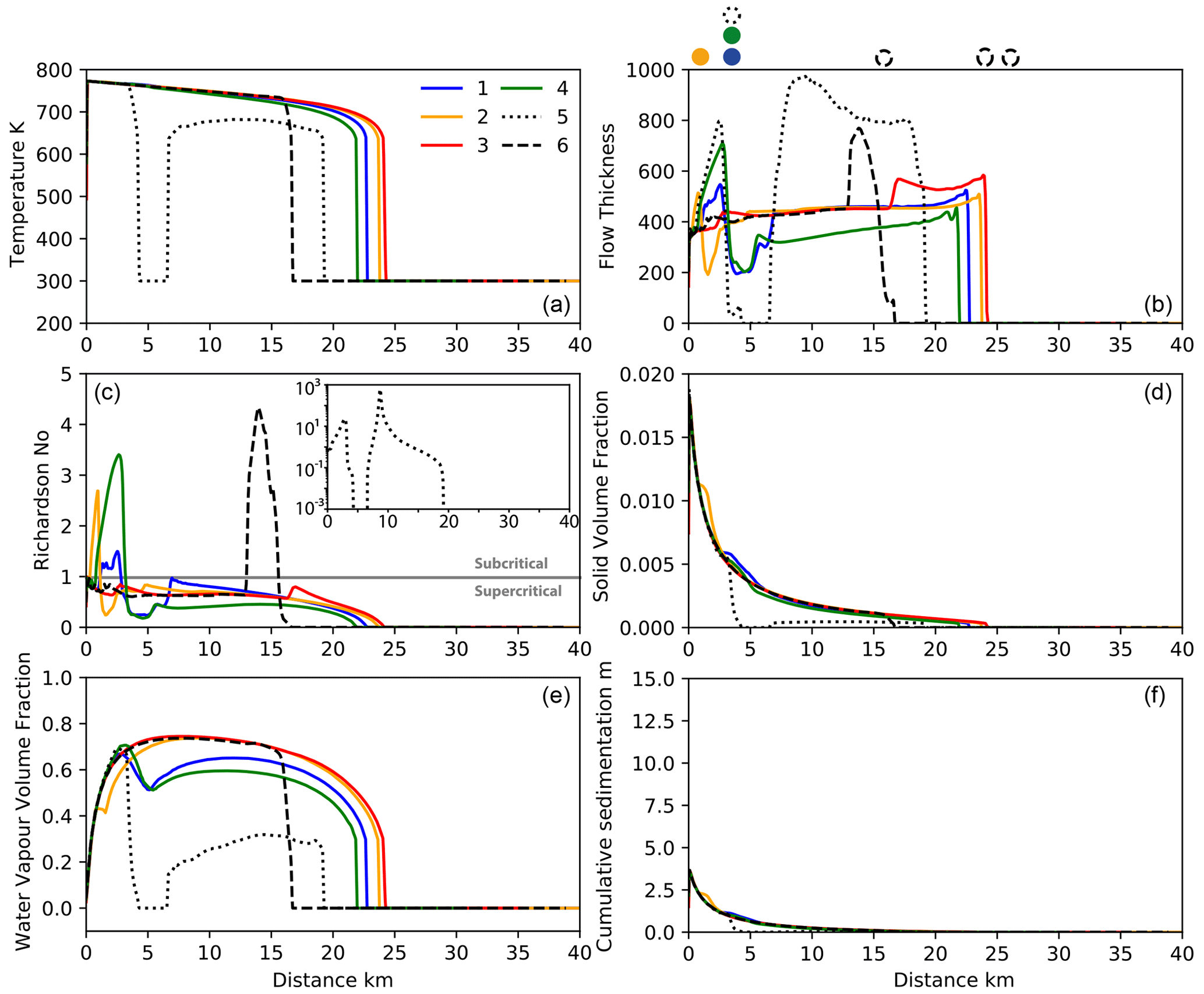
Figure 10 Variation in flow parameters with distance at 360 s after flow initiation for simulation SA4_0003, along transects shown in Fig. 8. Markers above panel (b) show the location of topographic barriers for each transect. The Richardson number with distance for transect 5 is shown in the inset.

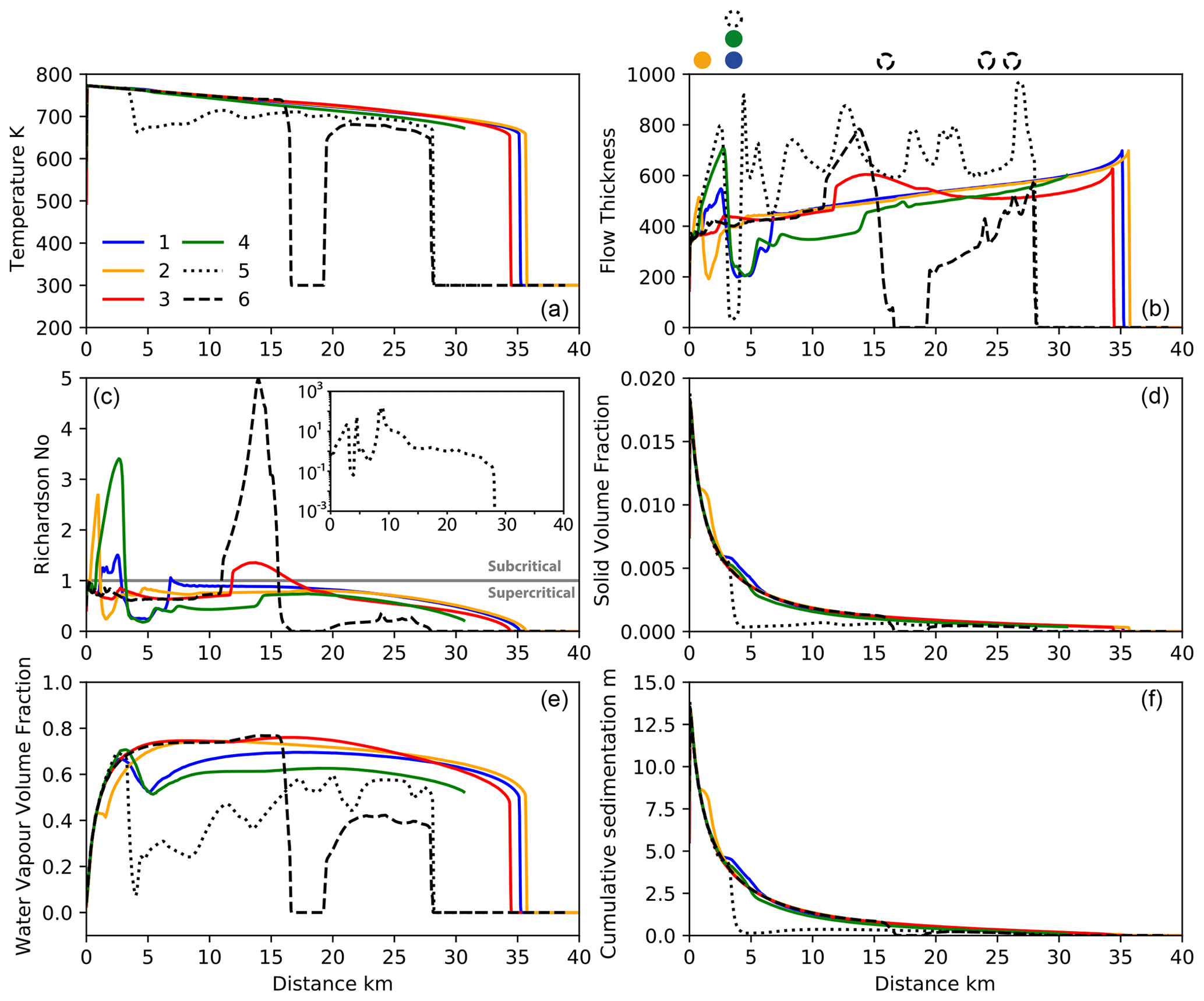
Figure 11 Variation in flow parameters with distance at 1320 s after flow initiation for simulation SA4_0003, along transects shown in Fig. 8. Markers above panel (b) show the location of topographic barriers for each transect. The Richardson number with distance for transect 5 is shown in the inset.

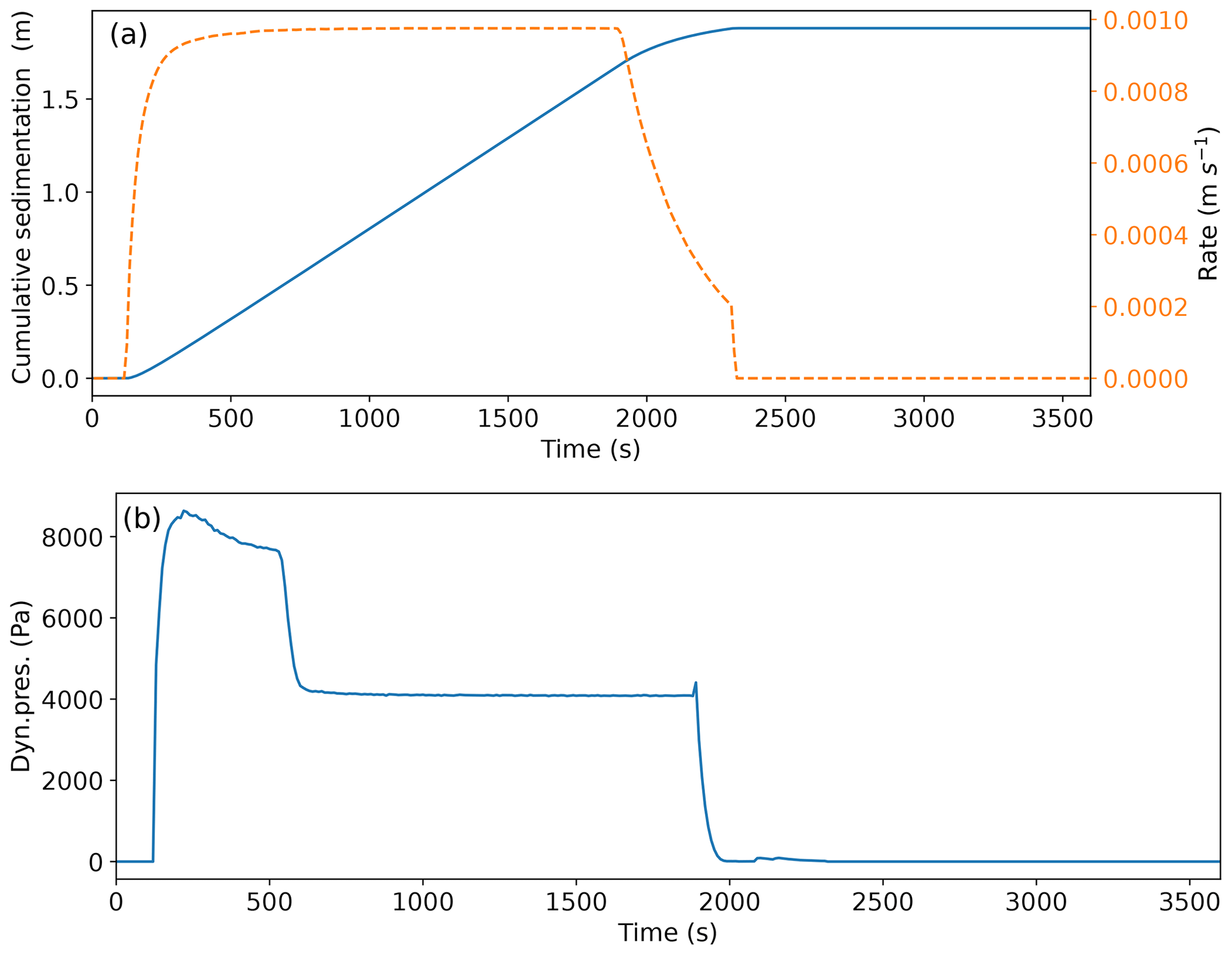
Figure 12 Variation in deposit thickness, rate and dynamic pressure at the probe location shown in Fig. 8.

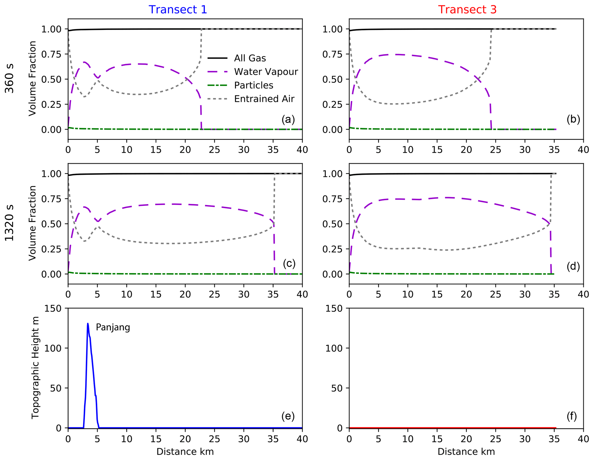
Figure 13 Variation in volume fraction of flow components along transects 1 and 3 at 360 and 1320 s after flow initiation.

The source condition of the simulated PDC mimics the initial radial spreading generated by a column collapse; the flow then quickly interacts with the nearby Krakatau islands of Sertung, Rakata and Panjang. The flow overtops the proximal islands of Sertung and Panjang, but it is directed around the much taller island of Rakata, with the flow fronts merging downstream on the far side of the island (Fig. 8). The flow runout at 360 and 1320 s varies along the different transects (Figs. 10 and 11), with runout considerably less along transects 5 and 6 than the other transects, related to the more variable topographic elevation along these transects (Fig. 9). Flow temperature shows a gradual decrease with distance from the source along most transects. The temperature drops to 300 K along transect 5 at 360 s and transect 6 at 1320 s. This reflects that at these times, there is no flow at these locations, and the temperature is that of the ambient.

In general, the simulated flow develops larger thicknesses at the head (Figs. 10, 11), followed by a thinner body. These changes are related to variations in the Ri number and air entrainment (Figs. 10, 11). In comparison to trends seen in Figs. 5 and 6 and results shown by Bursik and Woods (1996), Calabrò et al. (2022), and Shimizu et al. (2019, 2023), the trends do not show an initial decrease in thickness with distance. This is the result of the large volume of water vapour entrained into the flow, as shown in Fig. 11f. Numerical model results using smaller values for the ${\mathit{\gamma }}_{i_{\mathrm{s}},\mathrm{wv}}$ coefficient (Supplement Fig. S1) show a decrease in flow thickness with distance from the source. Flow thickness considerably increases upstream of topographic barriers, such as the islands of Sertung (transect 2) and Panjang (transect 1), which are within a couple of kilometres of the source. This increase is the result of the formation of backward-propagating hydraulic jumps, marking the transition from supercritical to subcritical flow. Downstream of topographic barriers, when the flows are capable of overcoming the obstacle, they transition back from thick, subcritical to thin supercritical flows. The most extreme variation in Richardson numbers occurs along transect 5 at 1320 s, with a high Richardson number upstream of Rakata, a topographic barrier to the flow, and a peak downstream of the island as the flow converges. This peak in Richardson number is due to a large decrease in velocity, which results in an increased loss of particles and therefore a decrease in the solid volume fraction within the flow (Fig. 10d).

Downstream of Rakata (transect 5), the flow thickness at 1320 s is highly variable, showing multiple peaks and troughs not directly associated with any variation in topography. These thickness variations are the result of the formation of von Kármán vortices that form in the wake of the topographic high on the island of Rakata, to the SE of the source (Fig. 11). Variations in the Richardson number for some transects match those shown in 1D simulations presented earlier in the paper (Fig. 4), whereby the transition from super- to subcritical flow moves upstream through time. This is shown particularly well for transect 6: at 360 s, the transition is clearly visible at a distance of approximately 13 km from the source (Fig. 11), while at 1320 s, it is less well defined and occurs approximately 2 km closer to the source (Fig. 11). This transition is also evident when studying the flow interactions with Sebesi, to the NE (Fig. 8): the shape of the hydraulic-jump front changes from tightly curved around the island at 360 s to a more elongate region at 600 s to a concave region bending back towards the Krakatau Archipelago at 1320 s. In Fig. 8 the backward propagation of the hydraulic jump is also evident when looking at the relative position of the transition region with respect to the red marker. This marker represents the probe location at which we sampled flow variables with time to show the effect of the passing hydraulic jump on current characteristics. In Fig. 12a we plot dynamic pressure and in Fig. 12b cumulative sedimentation and the sedimentation rate with time. These figures clearly show the arrival of the flow at 130 s. The dynamic pressure also shows the passing of the hydraulic jump at approximately 600 s (as also shown in Fig. 8c). The dynamic pressure shows a sharp decrease at approx. 1900 s, 100 s after source emission ends. Flow arrival at the probe location is also shown in Fig. 12b, with an increase in flow thickness and the sedimentation rate. After arrival of the flow, the sedimentation rate is almost constant, resulting in a linear increase in deposit thickness with time, with no change associated with the transition from supercritical to subcritical flow. The decay in sedimentation rate associated with the cessation of the flow is much more gentle than that of dynamic pressure. Variations in flow characteristics also occur along transect 3. At 360 s, transect 3 (Fig. 10b) shows a sharp increase in thickness at a distance of 16 km from the source that at later stages develops into a backward-propagating hydraulic jump. Figure 9 shows flat topography for this transect, but analysis of Fig. 8 shows that the increase in thickness is related to the flow interaction with the island of Sebesi.

Trends in deposit thickness closely follow those in solid volume fraction: both decrease exponentially with distance from the source (Figs. 10 and 11). The solid volume fraction and deposit thickness have slightly lower decay rates at distances of less than 2 and 5 km for transect 1 and 2, respectively, and more subtly at distances of approximately 5 km for transect 4. These increases relate to locations where the flow is in a subcritical regime; i.e. the flow is thicker and has higher Richardson numbers, equivalent to lower velocities. These slightly higher values of the solid volume fraction and consequently of sedimentation rates (see Eq. 19) are related to flow interaction with topography, whereby the flow slows and thickens and has higher sedimentation upstream of barriers. The solid volume fraction and deposit thickness trends differ significantly for transect 5, which has large changes in topographic elevation as it crosses the island of Rakata, close to the source. Both profiles show the same decay as seen in the other transects in the first couple of kilometres from the source, before decreasing sharply and, at distances of around 10 km from the source, showing a slight increase. These trends can be explained by the flow interaction with Rakata, which has a height of >700 m (Fig. 9). The flow is unable to overtop this barrier and instead flows around it, converging downstream. The decrease to a zero solid volume fraction and deposit thickness represents the sheltered part of Rakata that the flow does not reach (Figs. 10 and 11).

Figures 10f and 11f show a general increase and then decrease in the water vapour volume fraction of the flow with distance from the source. This is shown in greater detail in Fig. 13, where the water vapour volume fraction is plotted alongside the volume fractions of the other flow components. For the ${\mathit{\gamma }}_{i_{\mathrm{s}},\mathrm{wv}}$ coefficient used in this simulation, we can see that along both transects, the water vapour volume fraction can reach large values of up to almost 0.75. The relative amounts of water vapour and air also vary as the flows interact with topography, with transect 1 showing a decrease in water vapour and an increase in entrained air as the flow travels over Panjang to the east. Transect 3 shows steady variations in water vapour and entrained air, with the water vapour volume fraction quickly increasing and entrained air decreasing in the first couple of kilometres. There is then a gradual decrease in the amount of water vapour and an increase in entrained air over the next 15 km. This is related to a decrease in temperature towards the flow front, which results in lower thermal energy of the depositing particles available for seawater vaporization. The sharp decrease in water vapour and increase in air correspond to the flow front. Transect 3 does not intersect any topography, resulting in consistent trends with distance from the source at 360 s. However, at 1320 s, some subtle variation in both water vapour (a slight decrease) and the entrained air volume (a slight increase) fraction are seen between 10 and 15 km from the source. This is the result of the changing shape of the hydraulic jump that formed around the island of Sebesi. Additional simulations were performed to show the effect of the ${\mathit{\gamma }}_{i_{\mathrm{s}},\mathrm{wv}}$ coefficient on flow characteristics, and relevant figures are available in the Supplement.

A thorough discussion about the optimal choice of the rheological model and input parameters for PDCs, in particular those over water, requires an extensive comparison with phenomena and events at numerous volcanoes to accurately inform input parameters and sufficient observations with which to validate model results. More accurate measurements are needed to achieve a better calibration of the model. This, however, is beyond the scope of the present work.

7 Conclusions

We have presented developments to the physical model and the open-source numerical code IMEX_SfloW2D (de' Michieli Vitturi et al., 2019). They consist of the generalization of the shallow-water equations to describe a polydisperse fluid–solid mixture, including terms for sedimentation and entrainment of solids and water vapour, transport equations for solid particles of different sizes, transport equations for different components of the carrier phase, and an equation for temperature/energy. Constitutive equations allow us to adapt the numerical code to solve different types of geophysical mass flows (landslides, debris flows, lahars, snow and rock avalanches, pyroclastic avalanches), and here we have presented its application to the simulation of transient PDCs. The model resolves the depth-averaged flow velocity and density and does not account for the effects of internal flow stratification. In particular, it cannot be applied to PDCs in which the basal, concentrated flow interacts with the overlaying dilute ash cloud in a two-layer system (Shimizu et al., 2019). It is therefore suited to describing PDC end-members (either a concentrated pyroclastic avalanche or an inertial PDC). The numerical code has been tested to verify its capability to describe both sub- and supercritical regimes, as appropriate for large-scale, ignimbrite-forming eruptions. The results of synthetic numerical benchmarks demonstrate the robustness of the numerical code facing transcritical flows. Moreover, they highlight the importance of simulating transient in comparison to steady-state flows and flows in 2D versus 1D currents. Finally, the example application to Krakatau volcano shows the capability of the numerical model to face a complex natural case involving the propagation of PDCs over the sea surface and across topographic obstacles, showing the relevance, at a large scale, of non-linear fluid dynamic features, such as hydraulic jumps and von Kármán vortices. It is important to remark that, even if the 2D applications presented here are for radially spreading flows, the code is not restricted to these kinds of flows but can be applied, with the proper inlet conditions, to any kind of flow over a 2D topography.

In future versions of the code, we plan to adapt an approach similar to that presented for Newtonian laminar flows in Biagioli et al. (2021), where the depth-averaged equations have been modified to account for the vertical variation in velocity and temperature. The proposed modifications were implemented in the first version of IMEX-SfloW2D, and the applicability of such approaches to velocity and particle concentration profiles for dilute pyroclastic density currents has been shown in Keim and de' Michieli Vitturi (2022). Furthermore, in order to extend the range of the applications of the model and to allow for the numerical discretization of non-conservative terms, such as those appearing in multi-layer models and in approaches proposed in Fyhn et al. (2019) for the simulation of the constant velocity phase of channelized flows, we plan to implement the finite-volume schemes proposed in Diaz et al. (2019) in the code. We also point out that the present version of the code implements a rather simplified model for particle settling velocity, and in the future we plan to adopt more recent and accurate treatments for its calculations. For simple spheres, as assumed here, there are drag laws that avoid the jump in the Lun and Gidaspow drag law (Clift and Gauvin, 1971; Haider and Levenspiel, 1989), which can result in numerical problems when velocity is computed with an iterative numerical scheme. In addition, the use of a drag law for spheres in the case of natural sediments/volcanic particles is an important simplification that can lead to overestimating the terminal velocity and hence the sedimentation rate in the flow. We remark that the adoption of more complex models (Ganser, 1993; Bagheri and Bonadonna, 2016; Dioguardi et al., 2018) would also require knowledge of additional parameters characterizing the shape of the particles, which are not always easy to retrieve.

In conclusion, the depth-averaged model introduced in this study offers a promising avenue for advancing probabilistic volcanic hazard assessment. By providing a computationally efficient alternative to traditional 3D models, it significantly reduces the computational burden while still capturing, as shown by the Krakatau application, essential aspects of volcanic flows. For instance, for the simulation of the Krakatau case study for 1800 s, the code required 2 h of computational time on a seventh-generation Kaby Lake Intel Core i7 processor, which could be substantially reduced with a parallel run on multiple cores. Moreover, the utilization of a high-performance computing (HPC) system further amplifies the potential of the depth-averaged model in probabilistic volcanic hazard assessment, enabling the execution of a large number of simulations within a reasonable time frame. This makes the model well-suited for practical applications where timely hazard assessment is crucial.

Appendix A: Derivation of depth-averaged governing equations for variable density flows

In this part of the Appendix we present the derivation of the depth-averaged momentum and energy equations. For the sake of simplicity, we present the derivation by considering the ordinary gravity g, instead of the reduced gravity g^′, without friction terms. Furthermore, we present the derivation for a flow over a 1D topography parallel to the x axis. In this case, $B=B(x,t)$ and $h=h(x,t)$ are functions of x and t only, and the velocity vector is $\mathit{v}=(u,w)$, where u and w are the horizontal and vertical components, respectively (see Fig. A1).

A1 Momentum equation

The momentum equation is derived by integrating the Navier–Stokes equations in conservative form over the thickness of the flow and by applying appropriate boundary conditions at the top (free surface) and the bottom (topography) of the flow.

For a flow with no mass exchange with the surrounding environment and over an impermeable terrain constant in time ($\frac{\partial B}{\partial t}=\mathrm{0}$), the following kinematic conditions at the free surface and at the flow bottom (Johnson, 1997) are usually employed:

$$\begin{array}{ll}{\displaystyle \frac{\partial (B+h)}{\partial t}}& {\displaystyle }=w(x,B+h,t)-u(x,B+h,t){\displaystyle \frac{\partial (B+h)}{\partial x}}\\ {\displaystyle }& {\displaystyle }w(x,B,t)-u(x,B,t){\displaystyle \frac{\partial B}{\partial x}}=\mathrm{0}.\end{array}$$

The first condition states that the (moving) free surface must always be composed of fluid particles, i.e. that the free-surface elevation changes at a rate equal to the velocity of the flow in the direction perpendicular to the surface. The second condition states that the fluid velocity directed perpendicular to a solid boundary must vanish on the boundary itself.

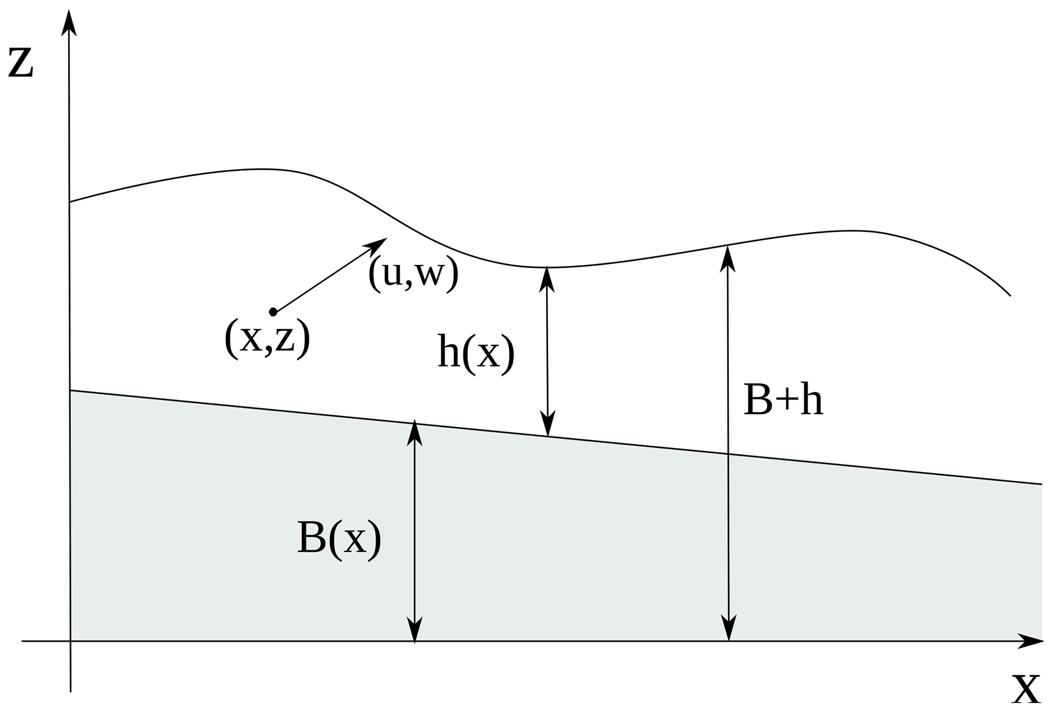
Figure A1 Model variables for a 1D flow. B is the topography elevation, h denotes flow thickness, and u and w are the horizontal and vertical components at the point (x,z).

However, here we consider atmospheric air entrainment and solid sedimentation, which affect both the topography and the free-surface elevations. For this reason, the classical equations presented above are modified in the following way:

$$\begin{array}{ll}{\displaystyle }& {\displaystyle \frac{\partial B}{\partial t}}+u(x,B,t){\displaystyle \frac{\partial B}{\partial x}}-w(x,B,t)=\sum _{i_{\mathrm{s}}=\mathrm{1}}^{n_{\mathrm{s}}}{S}_{\mathrm{s},i_{\mathrm{s}}},\\ {\displaystyle }& {\displaystyle \frac{\partial (B+h)}{\partial t}}+u(x,B+h,t){\displaystyle \frac{\partial (B+h)}{\partial x}}-w(x,B+h,t)=E_{\mathrm{a}}.\end{array}$$

In a 2D static Eulerian frame of reference (see Fig. A1), the momentum equation for the horizontal component of the velocity for a generic fluid parcel at the point (x,z) and with velocity (u,w), without shear stress and external forces, is written in the following way (Anderson, 1995, Eq. 2.42a):

$$\begin{array}{}\text{(A1)}& {\displaystyle \frac{\partial \left({\mathit{\rho }}_{\mathrm{m}}u\right)}{\partial t}}+{\displaystyle \frac{\partial \left({\mathit{\rho }}_{\mathrm{m}}{u}^{\mathrm{2}}\right)}{\partial x}}+{\displaystyle \frac{\partial \left({\mathit{\rho }}_{\mathrm{m}}uw\right)}{\partial y}}=-{\displaystyle \frac{\partial p}{\partial x}}.\end{array}$$

If we integrate between B and B+h on both sides of the equation, we can apply the Leibniz rule to the first term of the vertically integrated momentum conservation equation, obtaining

$$\begin{array}{ll}{\displaystyle }& {\displaystyle }\underset{B}{\overset{B+h}{\int }}{\displaystyle \frac{\partial \left({\mathit{\rho }}_{\mathrm{m}}u\right)}{\partial t}}\mathrm{d}t={\displaystyle \frac{\partial }{\partial t}}\underset{B}{\overset{B+h}{\int }}{\mathit{\rho }}_{\mathrm{m}}u\mathrm{d}z+{\mathit{\rho }}_{\mathrm{m}}u\left(B\right){\displaystyle \frac{\partial B}{\partial t}}\\ {\displaystyle }& {\displaystyle }-{\mathit{\rho }}_{\mathrm{m}}u(B+h){\displaystyle \frac{\partial (B+h)}{\partial t}}=\\ {\displaystyle }& {\displaystyle }{\displaystyle \frac{\partial }{\partial t}}\left({\mathit{\rho }}_{\mathrm{m}}h\overline{u}\right)+{\mathit{\rho }}_{\mathrm{m}}u\left(B\right){\displaystyle \frac{\partial B}{\partial t}}-{\mathit{\rho }}_{\mathrm{m}}u(B+h){\displaystyle \frac{\partial (B+h)}{\partial t}},\end{array}$$

where in the last equality we assumed that the density does not vary with depth and where we denoted with $\overline{u}$ the depth-averaged horizontal velocity:

$$\overline{u}={\displaystyle \frac{\mathrm{1}}{h}}\underset{B}{\overset{B+h}{\int }}u\mathrm{d}z.$$

In a similar way, we apply the Leibniz rule to the integral of the second term on the left-hand side of the momentum equation:

$$\begin{array}{ll}{\displaystyle }& {\displaystyle }\underset{B}{\overset{B+h}{\int }}{\displaystyle \frac{\partial \left({\mathit{\rho }}_{\mathrm{m}}{u}^{\mathrm{2}}\right)}{\partial x}}\mathrm{d}z={\displaystyle \frac{\partial }{\partial x}}\underset{B}{\overset{B+h}{\int }}{\mathit{\rho }}_{\mathrm{m}}{u}^{\mathrm{2}}\mathrm{d}z+{\mathit{\rho }}_{\mathrm{m}}{u}^{\mathrm{2}}\left(B\right){\displaystyle \frac{\partial B}{\partial x}}\\ {\displaystyle }& {\displaystyle }-{\mathit{\rho }}_{\mathrm{m}}{u}^{\mathrm{2}}(B+h){\displaystyle \frac{\partial (B+h)}{\partial x}}=\\ {\displaystyle }& {\displaystyle }{\displaystyle \frac{\partial \left({\mathit{\rho }}_{\mathrm{m}}h\overline{u^{\mathrm{2}}}\right)}{\partial x}}+{\mathit{\rho }}_{\mathrm{m}}{u}^{\mathrm{2}}\left(B\right){\displaystyle \frac{\partial B}{\partial x}}-{\mathit{\rho }}_{\mathrm{m}}{u}^{\mathrm{2}}(B+h){\displaystyle \frac{\partial (B+h)}{\partial x}},\end{array}$$

where we denote with $\overline{u^{\mathrm{2}}}$ the depth-averaged value of the square of the horizontal velocity as

$$\overline{u^{\mathrm{2}}}={\displaystyle \frac{\mathrm{1}}{h}}\underset{B}{\overset{B+h}{\int }}{u}^{\mathrm{2}}\mathrm{d}z.$$

For the integral of the last term on the left-hand side of the momentum equation, we can apply the fundamental theorem of calculus:

$${\displaystyle }\underset{B}{\overset{B+h}{\int }}{\displaystyle \frac{\partial {\mathit{\rho }}_{\mathrm{m}}uw}{\partial z}}\mathrm{d}z={\mathit{\rho }}_{\mathrm{m}}u(B+h)w(B+h)-{\mathit{\rho }}_{\mathrm{m}}u\left(B\right)w\left(B\right).$$

Thus, by summing the three terms, the integral of the left-hand side of the momentum Eq. (A1) is

$$\begin{array}{r}{\displaystyle \frac{\partial }{\partial t}}\left({\mathit{\rho }}_{\mathrm{m}}h\overline{u}\right)+{\displaystyle \frac{\partial }{\partial x}}\left({\mathit{\rho }}_{\mathrm{m}}h\overline{u^{\mathrm{2}}}\right)+{\mathit{\rho }}_{\mathrm{m}}\stackrel{\mathrm{̃}}{u}\left(B\right)\left[{\displaystyle \frac{\partial B}{\partial t}}+u\left(B\right){\displaystyle \frac{\partial B}{\partial x}}-w\left(B\right)\right]\\ -{\mathit{\rho }}_{\mathrm{m}}\stackrel{\mathrm{̃}}{u}(B+h)\left[{\displaystyle \frac{\partial (B+h)}{\partial t}}+w(B+h)-u(B+h){\displaystyle \frac{\partial (B+h)}{\partial x}}\right].\end{array}$$

In the previous equation, we denoted with the symbol $\stackrel{\mathrm{̃}}{u}$ the horizontal velocities at the bottom and at the free-surface interfaces. It is important to observe that at each of these interfaces we have two different velocities, one internal to the fluid and one external, and $\stackrel{\mathrm{̃}}{u}$ represents the velocity that contributes to the change in the terrain elevation or in the free-surface elevation. The first one changes because of particle sedimentation from the flow, so the velocity to consider is that of the flow. Conversely, the free-surface elevation change is associated with entrainment of atmospheric air, which we assume still. For this reason, $\stackrel{\mathrm{̃}}{u}(B+h)=\mathrm{0}$, and the last term is neglected, resulting in a simpler form of the integral of the left-hand side of the momentum equation:

$${\displaystyle \frac{\partial }{\partial t}}\left({\mathit{\rho }}_{\mathrm{m}}h\overline{u}\right)+{\displaystyle \frac{\partial }{\partial x}}\left({\mathit{\rho }}_{\mathrm{m}}h\overline{u^{\mathrm{2}}}\right)+{\mathit{\rho }}_{\mathrm{m}}u\left(B\right)\sum _{i_{\mathrm{s}}=\mathrm{1}}^{n_{\mathrm{s}}}{S}_{\mathrm{s},i_{\mathrm{s}}}.$$

For the integral of the right-hand side of the momentum equation (pressure term), we assume a hydrostatic pressure profile; i.e.

$$\begin{array}{}\text{(A2)}& p\left(x,z,t\right)=\underset{z}{\overset{B+h}{\int }}{\displaystyle \frac{\partial p\left(x,z,t\right)}{\partial z}}\mathrm{d}z=\mathit{\rho }g\left(B+h-z\right).\end{array}$$

To integrate the pressure term, we again apply the Leibniz rule to compute the term

$$\begin{array}{ll}{\displaystyle }& {\displaystyle }\underset{B}{\overset{B+h}{\int }}{\displaystyle \frac{\partial p\left(x,z,t\right)}{\partial x}}\mathrm{d}z={\displaystyle \frac{\partial }{\partial x}}\underset{B}{\overset{B+h}{\int }}p(x,z,t)\mathrm{d}z+p(x,B,t){\displaystyle \frac{\partial B}{\partial x}}\\ {\displaystyle }& {\displaystyle }-p(x,B+h,t){\displaystyle \frac{\partial }{\partial x}}(B+h)=\\ {\displaystyle }& {\displaystyle }{\displaystyle \frac{\partial }{\partial x}}{\left[-{\mathit{\rho }}_{\mathrm{m}}g{\displaystyle \frac{{\left(B+h-z\right)}^{\mathrm{2}}}{\mathrm{2}}}\right]}_B^{B+h}+{\mathit{\rho }}_{\mathrm{m}}gh{\displaystyle \frac{\partial B}{\partial x}}\\ {\displaystyle }& {\displaystyle }=-{\displaystyle \frac{\partial }{\partial x}}\left[{\mathit{\rho }}_{\mathrm{m}}g{\displaystyle \frac{h^{\mathrm{2}}}{\mathrm{2}}}\right]+{\mathit{\rho }}_{\mathrm{m}}gh{\displaystyle \frac{\partial B}{\partial x}}.\end{array}$$

If we assume that the vertical variations in the horizontal velocity are negligible, we can replace $\overline{u}$ and $\overline{u^{\mathrm{2}}}$ with u and u², respectively, where u represents the depth-averaged horizontal component of the velocity. With this assumption, combining the expression obtained for the integral of the left- and right-hand sides of the momentum equation, we obtain the following equation:

$$\begin{array}{}\text{(A3)}& \begin{array}{rl}& {\displaystyle \frac{\partial }{\partial t}}\left({\mathit{\rho }}_{\mathrm{m}}hu\right)+{\displaystyle \frac{\partial }{\partial x}}\left({\mathit{\rho }}_{\mathrm{m}}h{u}^{\mathrm{2}}\right)=-{\mathit{\rho }}_{\mathrm{m}}u\sum _{i_{\mathrm{s}}=\mathrm{1}}^{n_{\mathrm{s}}}{S}_{\mathrm{s},i_{\mathrm{s}}}\\ & +{\displaystyle \frac{\partial }{\partial x}}\left[{\mathit{\rho }}_{\mathrm{m}}g{\displaystyle \frac{h^{\mathrm{2}}}{\mathrm{2}}}\right]-{\mathit{\rho }}_{\mathrm{m}}gh{\displaystyle \frac{\partial B}{\partial x}}.\end{array}\end{array}$$

In Eq. (A2), for the sake of simplicity, we neglect the contribution of the atmospheric pressure to the hydrostatic pressure by assuming that the pressure is null at the free surface. When the contribution of the atmospheric pressure is considered, we obtain an equation with the reduced gravity instead of the ordinary gravity.

A2 Derivation of energy equation for variable density flows

In this part of the Appendix we present the derivation of the depth-averaged total energy equation, under the same assumption that led to the derivation of the depth-averaged momentum equation.

The desired equation is obtained by integrating over the flow depth the total energy equation for a 2D flow without shear stress (Anderson, 1995, Eq. 2.64):

$$\begin{array}{ll}{\displaystyle }& {\displaystyle \frac{\partial }{\partial t}}\left[{\mathit{\rho }}_{\mathrm{m}}\left(e+{\displaystyle \frac{u^{\mathrm{2}}+w^{\mathrm{2}}}{\mathrm{2}}}\right)\right]+{\displaystyle \frac{\partial }{\partial x}}\left[{\mathit{\rho }}_{\mathrm{m}}\left(e+{\displaystyle \frac{u^{\mathrm{2}}+w^{\mathrm{2}}}{\mathrm{2}}}\right)u\right]\\ {\displaystyle }& {\displaystyle }+{\displaystyle \frac{\partial }{\partial z}}\left[{\mathit{\rho }}_{\mathrm{m}}\left(e+{\displaystyle \frac{u^{\mathrm{2}}+w^{\mathrm{2}}}{\mathrm{2}}}\right)w\right]=-{\displaystyle \frac{\partial \left(up\right)}{\partial x}}-{\displaystyle \frac{\partial \left(wp\right)}{\partial z}}+w{\mathit{\rho }}_{\mathrm{m}}g,\end{array}$$

where e=C_vT is the internal energy of the flow.

By using the Leibniz rule, the integral of the first term of the left-hand side of the energy equation is

$$\begin{array}{ll}{\displaystyle }& {\displaystyle }\underset{B}{\overset{B+h}{\int }}{\displaystyle \frac{\partial }{\partial t}}\left[{\mathit{\rho }}_{\mathrm{m}}\left(e+{\displaystyle \frac{u^{\mathrm{2}}+w^{\mathrm{2}}}{\mathrm{2}}}\right)\right]\mathrm{d}z=\\ {\displaystyle }& {\displaystyle }{\displaystyle \frac{\partial }{\partial t}}\underset{B}{\overset{B+h}{\int }}\left[{\mathit{\rho }}_{\mathrm{m}}\left(e+{\displaystyle \frac{u^{\mathrm{2}}+w^{\mathrm{2}}}{\mathrm{2}}}\right)\right]\mathrm{d}z\\ {\displaystyle }& {\displaystyle }+{\left[{\mathit{\rho }}_{\mathrm{m}}\left(e+{\displaystyle \frac{u^{\mathrm{2}}+w^{\mathrm{2}}}{\mathrm{2}}}\right)\right]}_{z=B}{\displaystyle \frac{\partial B}{\partial t}}\\ {\displaystyle }& {\displaystyle }-{\left[{\mathit{\rho }}_{\mathrm{m}}\left(e+{\displaystyle \frac{u^{\mathrm{2}}+w^{\mathrm{2}}}{\mathrm{2}}}\right)\right]}_{z=B+h}{\displaystyle \frac{\partial (B+h)}{\partial t}}.\end{array}$$

Proceeding in a similar way, the second term can be written as

$$\begin{array}{ll}{\displaystyle }& {\displaystyle }\underset{B}{\overset{B+h}{\int }}{\displaystyle \frac{\partial }{\partial x}}\left[{\mathit{\rho }}_{\mathrm{m}}\left(e+{\displaystyle \frac{u^{\mathrm{2}}+w^{\mathrm{2}}}{\mathrm{2}}}\right)u\right]\mathrm{d}z=\\ {\displaystyle }& {\displaystyle }{\displaystyle \frac{\partial }{\partial x}}\underset{B}{\overset{B+h}{\int }}\left[{\mathit{\rho }}_{\mathrm{m}}\left(e+{\displaystyle \frac{u^{\mathrm{2}}+w^{\mathrm{2}}}{\mathrm{2}}}\right)u\right]\mathrm{d}z\\ {\displaystyle }& {\displaystyle }{\left[{\mathit{\rho }}_{\mathrm{m}}\left(e+{\displaystyle \frac{u^{\mathrm{2}}+w^{\mathrm{2}}}{\mathrm{2}}}\right)u\right]}_{z=B}{\displaystyle \frac{\partial B}{\partial x}}\\ {\displaystyle }& {\displaystyle }-{\left[{\mathit{\rho }}_{\mathrm{m}}\left(e+{\displaystyle \frac{u^{\mathrm{2}}+w^{\mathrm{2}}}{\mathrm{2}}}\right)u\right]}_{z=B+h}{\displaystyle \frac{\partial (B+h)}{\partial x}}.\end{array}$$

For the integration of the third term of the left-hand side, we apply the fundamental theorem of calculus:

$$\begin{array}{ll}{\displaystyle }& {\displaystyle }\underset{B}{\overset{B+h}{\int }}{\displaystyle \frac{\partial }{\partial z}}\left[{\mathit{\rho }}_{\mathrm{m}}\left(e+{\displaystyle \frac{u^{\mathrm{2}}+w^{\mathrm{2}}}{\mathrm{2}}}\right)w\right]\mathrm{d}z=\\ {\displaystyle }& {\displaystyle }{\left[{\mathit{\rho }}_{\mathrm{m}}\left(e+{\displaystyle \frac{u^{\mathrm{2}}+w^{\mathrm{2}}}{\mathrm{2}}}\right)w\right]}_{z=B+h}-{\left[{\mathit{\rho }}_{\mathrm{m}}\left(e+{\displaystyle \frac{u^{\mathrm{2}}+w^{\mathrm{2}}}{\mathrm{2}}}\right)w\right]}_{z=B}.\end{array}$$

If we assume that T, ρ_m and u do not vary with depth, then we can write the left-hand side of the energy equation in the following way:

$$\begin{array}{ll}{\displaystyle }& {\displaystyle \frac{\partial }{\partial t}}\left[{\mathit{\rho }}_{\mathrm{m}}h\left(e+{\displaystyle \frac{\stackrel{\mathrm{‾}}{u^{\mathrm{2}}}+\stackrel{\mathrm{‾}}{w^{\mathrm{2}}}}{\mathrm{2}}}\right)\right]+{\displaystyle \frac{\partial }{\partial x}}\left[{\mathit{\rho }}_{\mathrm{m}}h\left(e\overline{u}+{\displaystyle \frac{\stackrel{\mathrm{‾}}{u^{\mathrm{3}}}+\stackrel{\mathrm{‾}}{u{w}^{\mathrm{2}}}}{\mathrm{2}}}\right)\right]\\ {\displaystyle }& {\displaystyle }-{\left[{\mathit{\rho }}_{\mathrm{m}}\left(e+{\displaystyle \frac{u^{\mathrm{2}}+w^{\mathrm{2}}}{\mathrm{2}}}\right)\right]}_{z=B+h}\\ {\displaystyle }& {\displaystyle }\left[{\displaystyle \frac{\partial (B+h)}{\partial t}}+u(B+h){\displaystyle \frac{\partial (B+h)}{\partial x}}-w(B+h)\right]\\ {\displaystyle }& {\displaystyle }+{\left[{\mathit{\rho }}_{\mathrm{m}}\left(e+{\displaystyle \frac{u^{\mathrm{2}}+w^{\mathrm{2}}}{\mathrm{2}}}\right)\right]}_{z=B}\left[{\displaystyle \frac{\partial B}{\partial t}}+u\left(B\right){\displaystyle \frac{\partial B}{\partial x}}-w\left(B\right)\right].\end{array}$$

As for the momentum equation, we observe that the terms in the square brackets depending on the free-surface and topography elevation are associated with air entrainment and particle sedimentation rates. Furthermore, it is important to remark that air entrainment does not carry any kinetic energy in the flow but only thermal energy, and both energies are lost due to particle sedimentation. With this in mind, we can rewrite the equation above in the following way:

$$\begin{array}{l}{\displaystyle \frac{\partial }{\partial t}}\left[{\mathit{\rho }}_{\mathrm{m}}h\left(e+{\displaystyle \frac{\stackrel{\mathrm{‾}}{u^{\mathrm{2}}}+\stackrel{\mathrm{‾}}{w^{\mathrm{2}}}}{\mathrm{2}}}\right)\right]+{\displaystyle \frac{\partial }{\partial x}}\left[{\mathit{\rho }}_{\mathrm{m}}h\left(e\overline{u}+{\displaystyle \frac{\stackrel{\mathrm{‾}}{u^{\mathrm{3}}}+\stackrel{\mathrm{‾}}{u{w}^{\mathrm{2}}}}{\mathrm{2}}}\right)\right]\\ {\displaystyle }-{\mathit{\rho }}_{\mathrm{a}}{C}_{\mathrm{a}}{T}_{\mathrm{a}}{E}_{\mathrm{a}}+\sum _{i_{\mathrm{s}}=\mathrm{1}}^{n_{\mathrm{s}}}\left[{\mathit{\rho }}_{\mathrm{s},i_{\mathrm{s}}}\left(C_{\mathrm{s},i_{\mathrm{s}}}T+{\displaystyle \frac{u(B{)}^{\mathrm{2}}+w(B{)}^{\mathrm{2}}}{\mathrm{2}}}\right)\right]S_{\mathrm{s},i_{\mathrm{s}}}.\end{array}$$

We compute now the integral of the pressure and gravitational terms. The first term on the right-hand side of the energy equation can be integrated by applying the Leibniz rule:

$$\begin{array}{ll}{\displaystyle }& {\displaystyle }\underset{B}{\overset{B+h}{\int }}{\displaystyle \frac{\partial \left(up\right)}{\partial x}}\mathrm{d}z={\displaystyle \frac{\partial }{\partial x}}\underset{B}{\overset{B+h}{\int }}p(x,z,t)u(x,z,t)\mathrm{d}z\\ {\displaystyle }& {\displaystyle }+p(x,B,t)u(x,B,t){\displaystyle \frac{\partial B}{\partial x}}\\ {\displaystyle }& {\displaystyle }-p(x,B+h,t)u(x,B+h,t){\displaystyle \frac{\partial (B+h)}{\partial x}}=\\ {\displaystyle }& {\displaystyle \frac{\partial }{\partial x}}\underset{B}{\overset{B+h}{\int }}p(x,z,t)u(x,z,t)\mathrm{d}z+{\mathit{\rho }}_{\mathrm{m}}ghu\left(B\right){\displaystyle \frac{\partial B}{\partial x}}.\end{array}$$

In the second equality, the last term on the left-hand side is null because we assumed the hydrostatic pressure is null at the free surface. In the equation above, the integral of the product of the pressure and the horizontal velocity is computed by approximating the horizontal velocity with $\overline{u}$ and by substituting $p\left(z\right)={\mathit{\rho }}_{\mathrm{m}}g(B+h-z)$, obtaining

$$\begin{array}{ll}{\displaystyle }& {\displaystyle \frac{\partial }{\partial x}}\underset{B}{\overset{B+h}{\int }}p(x,z,t)\overline{u}(x,t)\mathrm{d}z=\\ {\displaystyle }& {\displaystyle \frac{\partial }{\partial x}}\left[u(x,t)\underset{B}{\overset{B+h}{\int }}{\mathit{\rho }}_{\mathrm{m}}g(B+h-z)\mathrm{d}z\right]={\displaystyle \frac{\partial }{\partial x}}\left[{\mathit{\rho }}_{\mathrm{m}}g\overline{u}{\displaystyle \frac{h^{\mathrm{2}}}{\mathrm{2}}}\right].\end{array}$$

The second pressure term on the right-hand side of the energy equation, when integrated over the flow depth, is

$$\begin{array}{ll}{\displaystyle }& {\displaystyle }\underset{B}{\overset{B+h}{\int }}{\displaystyle \frac{\partial \left(wp\right)}{\partial z}}\mathrm{d}z=p(x,B+h,t)w(x,B+h,t)\\ {\displaystyle }& {\displaystyle }-p(x,B,t)w(x,B,t)=-{\mathit{\rho }}_{\mathrm{m}}ghw(B+h).\end{array}$$

This term, if we assume that the variations in the vertical component of the velocity with flow depth are negligible, cancels out with the integral of the work done by the gravitational force:

$$\underset{B}{\overset{B+h}{\int }}w{\mathit{\rho }}_{\mathrm{m}}g={\mathit{\rho }}_{\mathrm{m}}gh\overline{w}.$$

Now, if we sum all the terms, we have

$$\begin{array}{ll}{\displaystyle }& {\displaystyle \frac{\partial }{\partial t}}\left[{\mathit{\rho }}_{\mathrm{m}}h\left(e+{\displaystyle \frac{\stackrel{\mathrm{‾}}{u^{\mathrm{2}}}+\stackrel{\mathrm{‾}}{w^{\mathrm{2}}}}{\mathrm{2}}}\right)\right]+{\displaystyle \frac{\partial }{\partial x}}\left[{\mathit{\rho }}_{\mathrm{m}}h\left(e\overline{u}+{\displaystyle \frac{\stackrel{\mathrm{‾}}{u^{\mathrm{3}}}+\stackrel{\mathrm{‾}}{u{w}^{\mathrm{2}}}}{\mathrm{2}}}\right)\right]\\ {\displaystyle }& {\displaystyle }+{\displaystyle \frac{\partial }{\partial x}}\left[{\mathit{\rho }}_{\mathrm{m}}g\overline{u}{\displaystyle \frac{h^{\mathrm{2}}}{\mathrm{2}}}\right]=-{\mathit{\rho }}_{\mathrm{m}}ghu\left(B\right){\displaystyle \frac{\partial B}{\partial x}}\\ {\displaystyle }& {\displaystyle }-{\mathit{\rho }}_{\mathrm{a}}{C}_{\mathrm{a}}{T}_{\mathrm{a}}{E}_{\mathrm{a}}+\sum _{i_{\mathrm{s}}=\mathrm{1}}^{n_{\mathrm{s}}}\left[{\mathit{\rho }}_{\mathrm{s},i_{\mathrm{s}}}\left(C_{\mathrm{s},i_{\mathrm{s}}}T+{\displaystyle \frac{u(B{)}^{\mathrm{2}}+w(B{)}^{\mathrm{2}}}{\mathrm{2}}}\right)\right]S_{\mathrm{s},i_{\mathrm{s}}}.\end{array}$$

If we neglect the contribution of the vertical component of the velocity to the kinetic energy and we assume that the horizontal velocity is constant ($u\left(z\right)=\overline{u}$), we have

$$\begin{array}{ll}{\displaystyle }& {\displaystyle \frac{\partial }{\partial t}}\left[{\mathit{\rho }}_{\mathrm{m}}h\left(e+{\displaystyle \frac{u^{\mathrm{2}}}{\mathrm{2}}}\right)\right]+{\displaystyle \frac{\partial }{\partial x}}\left[{\mathit{\rho }}_{\mathrm{m}}hu\left(e+{\displaystyle \frac{u^{\mathrm{2}}}{\mathrm{2}}}\right)+{\mathit{\rho }}_{\mathrm{m}}gu{\displaystyle \frac{h^{\mathrm{2}}}{\mathrm{2}}}\right]=\\ {\displaystyle }& {\displaystyle }-{\mathit{\rho }}_{\mathrm{m}}ghu{\displaystyle \frac{\partial B}{\partial x}}+{\mathit{\rho }}_{\mathrm{a}}{C}_{\mathrm{a}}{T}_{\mathrm{a}}{E}_{\mathrm{a}}\\ {\displaystyle }& {\displaystyle }-\sum _{i_{\mathrm{s}}=\mathrm{1}}^{n_{\mathrm{s}}}\left[{\mathit{\rho }}_{\mathrm{s},i_{\mathrm{s}}}\left(C_{\mathrm{s},i_{\mathrm{s}}}T+{\displaystyle \frac{u(B{)}^{\mathrm{2}}+w(B{)}^{\mathrm{2}}}{\mathrm{2}}}\right)\right]S_{\mathrm{s},i_{\mathrm{s}}}.\end{array}$$

By neglecting the vertical component of the velocity we have a small error in the kinetic energy. For this reason, when the equation for the total energy is solved and the temperature is computed from the total energy, a small error is also present in the temperature.

A3 Derivation of primitive variables from conservative variables

The model solves for the following set of conservative variables:

$$\begin{array}{}\text{(A4)}& \begin{array}{rl}\mathbf{Q}& =\left(Q_{\mathrm{1}},\mathrm{\dots },Q_{\mathrm{5}+n_{\mathrm{s}}}\right)=({\mathit{\rho }}_{\mathrm{m}}h,{\mathit{\rho }}_{\mathrm{m}}hu,{\mathit{\rho }}_{\mathrm{m}}hv,{\mathit{\rho }}_{\mathrm{m}}eh,\\ & h{\mathit{\rho }}_{{\mathrm{s}}_{\mathrm{1}}}{\mathit{\alpha }}_{{\mathrm{s}}_{\mathrm{1}}},\mathrm{\dots },h{\mathit{\rho }}_{{\mathrm{s}}_{\mathrm{n}}}{\mathit{\alpha }}_{{\mathrm{s}}_{\mathrm{n}}},h{\mathit{\rho }}_{\mathrm{wv}}{\mathit{\alpha }}_{\mathrm{wv}}).\end{array}\end{array}$$

In order to evaluate the fluxes and the other terms in the governing equations, we need to write, in terms of $\left(Q_{\mathrm{1}},\mathrm{\dots },Q_{\mathrm{4}+n_{\mathrm{s}}}\right)$, the primitive variable $\mathbf{P}=(h,hu,hv,T,{\mathit{\alpha }}_{{\mathrm{s}}_{\mathrm{1}}},\mathrm{\dots },{\mathit{\alpha }}_{n_{\mathrm{s}}},u,v)$, which completely defines the state. In this part of the Appendix we describe the procedure implemented in the code to compute these quantities from the conservative variables.

First of all, mass fractions of solid phases and water vapour are computed as

$$\begin{array}{}\text{(A5)}& x_{\mathrm{s},i_{\mathrm{s}}}={\displaystyle \frac{Q_{\mathrm{4}+i_{\mathrm{s}}}}{Q_{\mathrm{1}}}}{i}_{\mathrm{s}}=\mathrm{1},\mathrm{\dots },n_{\mathrm{s}}{x}_{\mathrm{wv}}={\displaystyle \frac{Q_{\mathrm{5}+n_{\mathrm{s}}}}{Q_{\mathrm{1}}}},\end{array}$$

and these allow us to also obtain the mass fraction of air:

$$\begin{array}{}\text{(A6)}& x_{\mathrm{a}}=\mathrm{1}-\sum _{i_{\mathrm{s}}=\mathrm{1}}^{n_S}{x}_{\mathrm{s},i_{\mathrm{s}}}-x_{\mathrm{wv}}.\end{array}$$

In this way, mass-averaged quantities of the averaged specific heat C_v can be written in the following way:

$$\begin{array}{}\text{(A7)}& C_{\mathrm{mix}}=\sum _{i_{\mathrm{s}}=\mathrm{1}}^{n_{\mathrm{s}}}{x}_{\mathrm{s},i_{\mathrm{s}}}{C}_{\mathrm{s},i_{\mathrm{s}}}+x_{\mathrm{wv}}{C}_{\mathrm{wv}}+x_{\mathrm{a}}{C}_{\mathrm{a}}.\end{array}$$

Once the average specific heat is known, temperature can be computed from the total specific energy, expressed by Q₄, in the following way:

$$\begin{array}{}\text{(A8)}& \begin{array}{rl}h{\mathit{\rho }}_{\mathrm{m}}{C}_{\mathrm{v}}T& =\left[Q_{\mathrm{4}}-{\displaystyle \frac{Q_{\mathrm{2}}^{\mathrm{2}}+Q_{\mathrm{3}}^{\mathrm{2}}}{\mathrm{2}{Q}_{\mathrm{1}}}}\right]\\ & \Rightarrow T={\displaystyle \frac{\mathrm{1}}{Q_{\mathrm{1}}{C}_{\mathrm{v}}}}\left[Q_{\mathrm{4}}-{\displaystyle \frac{Q_{\mathrm{2}}^{\mathrm{2}}+Q_{\mathrm{3}}^{\mathrm{2}}}{\mathrm{2}{Q}_{\mathrm{1}}}}\right].\end{array}\end{array}$$

From the temperature it is possible, through the equation of state, to calculate the density of air (${\mathit{\rho }}_{\mathrm{a}}=\frac{P}{R_{\mathrm{a}}T}$) and water vapour (${\mathit{\rho }}_{\mathrm{wv}}=\frac{P}{R_{\mathrm{wv}}T}$) and then the density of the mixture:

$$\begin{array}{}\text{(A9)}& {\displaystyle \frac{\mathrm{1}}{{\mathit{\rho }}_{\mathrm{mix}}}}=\sum _{i_{\mathrm{s}}=\mathrm{1}}^{n_{\mathrm{s}}}{\displaystyle \frac{x_{\mathrm{s},i_{\mathrm{s}}}}{{\mathit{\rho }}_{\mathrm{s},i_{\mathrm{s}}}}}+{\displaystyle \frac{x_{\mathrm{a}}}{{\mathit{\rho }}_{\mathrm{a}}}}+{\displaystyle \frac{x_{\mathrm{wv}}}{{\mathit{\rho }}_{\mathrm{wv}}}}.\end{array}$$

Mixture density is used to compute flow thickness and volume fractions:

$$\begin{array}{}\text{(A10)}& \begin{array}{rl}& h={\displaystyle \frac{Q_{\mathrm{1}}}{{\mathit{\rho }}_{\mathrm{mix}}}},{\mathit{\alpha }}_{\mathrm{s},i_{\mathrm{s}}}={\displaystyle \frac{x_{\mathrm{s},i_{\mathrm{s}}}{\mathit{\rho }}_{\mathrm{mix}}}{{\mathit{\rho }}_{\mathrm{s},i_{\mathrm{s}}}}},{\mathit{\alpha }}_{\mathrm{wv}}={\displaystyle \frac{x_{\mathrm{wv}}{\mathit{\rho }}_{\mathrm{mix}}}{{\mathit{\rho }}_{\mathrm{wv}}}},\\ & {\mathit{\alpha }}_{\mathrm{a}}={\displaystyle \frac{x_{\mathrm{a}}{\mathit{\rho }}_{\mathrm{mix}}}{{\mathit{\rho }}_{\mathrm{a}}}}.\end{array}\end{array}$$

Flow velocities are computed from the conservative variables. Here, as done in Kurganov and Petrova (2007), a desingularization is applied in order to avoid division by very small numbers and thus velocities that are too large:

$$\begin{array}{}\text{(A11)}& u={\displaystyle \frac{\sqrt{\mathrm{2}}{Q}_{\mathrm{1}}{Q}_{\mathrm{2}}}{\sqrt{Q_{\mathrm{1}}^{\mathrm{4}}+max(Q_{\mathrm{1}}^{\mathrm{4}},\mathit{ϵ})}}},v={\displaystyle \frac{\sqrt{\mathrm{2}}{Q}_{\mathrm{1}}{Q}_{\mathrm{3}}}{\sqrt{Q_{\mathrm{1}}^{\mathrm{4}}+max(Q_{\mathrm{1}}^{\mathrm{4}},\mathit{ϵ})}}}.\end{array}$$

Finally, volumetric fluxes hu and hv are not computed directly from the conservative variables but from the primitive variables obtained from Eqs. (A10) and (A11):

$$\begin{array}{}\text{(A12)}& hu=h\cdot u,hu=h\cdot v.\end{array}$$