the Creative Commons Attribution 4.0 License.
the Creative Commons Attribution 4.0 License.
 | 07 Nov 2023
CIOFC1.0: a common parallel input/output framework based on C-Coupler2.0
Xinzhu Yu
Li Liu
Chao Sun
Qingu Jiang
Biao Zhao
Zhiyuan Zhang
Bin Wang
As earth system modeling develops ever finer grid resolutions, the inputting and outputting (I/O) of the increasingly large data fields becomes a processing bottleneck. Many models developed in China, as well as the community coupler (C-Coupler), do not fully benefit from existing parallel I/O supports. This paper reports the design and implementation of a common parallel input/output framework (CIOFC1.0) based on C-Coupler2.0. The CIOFC1.0 framework can accelerate the I/O of large data fields by parallelizing data read/write operations among processes. The framework also allows convenient specification by users of the I/O settings, e.g., the data fields for I/O, the time series of the data files for I/O, and the data grids in the files. The framework can also adaptively input data fields from a time series dataset during model integration, automatically interpolate data when necessary, and output fields either periodically or irregularly. CIOFC1.0 demonstrates the cooperative development of an I/O framework and coupler, and thus enables convenient and simultaneous use of a coupler and an I/O framework.
- Article
(2205 KB) - Full-text XML
- BibTeX
- EndNote


Earth system models generally integrate component models of the atmosphere, ocean, land surface, and sea ice to support climate change studies and provide seamless numerical predictions (Brunet et al., 2015). A coupler is a significant component or library in an earth system model that effectively handles coupling among the component models. The various families of coupler include MCT (Model Coupling Toolkit) (Larson et al., 2005), OASIS (Ocean Atmosphere Sea Ice Soil) (Redler et al., 2010; Valcke, 2013; Craig et al., 2017), CPL (CESM coupler) (Craig et al., 2005, 2012), YAC (Yet Another Coupler) (Hanke et al., 2016), and C-Coupler (community coupler) (Liu et al., 2014, 2018). There are also model frameworks with coupler capabilities, such as ESMF (Earth System Modeling Framework) (Valcke et al., 2012) and FMS (Flexible Modeling System) (Balaji et al., 2006). This paper focuses on C-Coupler, a coupler family developed in, and widely used in, China (Li et al., 2020b; Lin et al., 2020; Shi et al., 2022; Ren et al., 2021; Wang et al., 2018; Zhao et al., 2017).
As models are using finer grid resolutions, both they and the associated couplers are required to input and output (I/O) increasingly large data files, and I/O becomes a bottleneck in model simulations. Besides the fundamental supports, such as MPI-IO (Message Passing Interface-IO) and PnetCDF (Parallel Network Common Data Format; Li et al., 2003), a set of parallel I/O libraries and frameworks have been developed for models, e.g., the PIO (parallel I/O) library (Dennis et al., 2011) used by CESM and other climate models, the SCORPIO (Software for Caching Output and Reads for Parallel I/O) library (Krishna et al., 2020) used by the E3SM climate model, a parallel I/O library used in a global cloud resolving model (Palmer et al., 2011), the ADIOS (Adaptable Input Output System) library (Godoy et al., 2020) used by the GRAPES (Global/Regional Assimilation and Prediction System; Zou et al., 2014) model, the I/O library used by the ESMF framework, and the CFIO (Climate Fast Input/Output) library (Huang et al., 2014). XIOS (XML Input/Output Server) (Yepes-Arbós et al., 2018) can be viewed as a common I/O framework that provides XML configuration files, has parallel and asynchronous I/O capability, and can automatically handle data interpolation between different grids when required. It has been used in the IFS (integrated forecasting system) CY43R3.
However, many models developed in China do not fully benefit from parallel I/O supports, and instead use sequential I/O for high-resolution model output, e.g., the GAMIL (grid-point atmospheric model of IAP LASG) atmosphere model (L. Li et al., 2013a, b, 2020a) and C-Coupler. To assist in model development in China, this paper reports the design and development of the common parallel I/O framework based on C-Coupler2.0 (CIOFC1.0). The framework can benefit not only C-Coupler but also various component models. The remainder of this paper is organized as follows: Sects. 2 and 3 introduce the overall design and the implementation of CIOFC1.0, respectively. The framework is evaluated in Sect. 4, and a discussion and the conclusions are provided in Sect. 5.
With the aim of aiding model development, we considered the following main requirements when designing the new I/O framework:
-
The framework can obviously accelerate data input and output by employing parallel I/O supports, especially under a fine resolution.
-
The framework should adaptively input time series data fields from a set of data files and automatically conduct time interpolation when required.
-
The framework should facilitate outputting of data either periodically or irregularly. Periodic output is a traditional requirement, but atmospheric models such as GRAPES (Zhang and Shen, 2008), which is now used for national operational weather forecasting in China, does not use a uniform period for data output: it generally outputs data for 3 h intervals in the first 5 model days and then for 6 h intervals in the remaining model days. The atmospheric chemistry model GEOS-Chem (Long et al., 2015) enables users to specify a set of specific model dates for outputting model data.
-
The framework should automatically conduct spatial interpolation in parallel when a data field is on different grids in the model and in the data files. Users generally expect fields in data files to be on regular grids (particularly longitude–latitude grids), while models increasingly employ irregular grids. For example, the atmospheric model of FV3 (Finite Volume Cubed Sphere) (Putman and Lin, 2007) and MCV (Multimoment Constrained Finite-Volume Model) (X. Li et al., 2013; Chen et al., 2014; Tang et al., 2021) use cubed-sphere grids, the atmospheric model MPAS-A (Heinzeller et al., 2016) generally uses unstructured grids generated by triangulation (Jacobsen et al., 2013; Yang et al., 2019), and many ocean models (e.g., POP (Parallel Ocean Program) (Smith et al., 2010), LICOM (LASG/IAP climate system ocean model) (Lin et al., 2016; Liu et al., 2012), and MOM (Modular Ocean Model) (Griffies, 2012)) use tripolar grids. Spatial interpolation therefore becomes necessary when inputting and outputting data fields for models.
-
The framework should facilitate flexible and convenient specification of the I/O settings, e.g., the data fields to be input or output, the time series of the input data files or of the output data, and the data grids in files (called “file grids” hereafter).
We designed the main architecture of CIOFC1.0 considering the above requirements. Figure 1 shows that it comprises the following set of modules: input time series manager, output time series manager, spatial data interpolation manager, parallel I/O operation, output driving procedure, input driving procedure, and I/O configuration manager. These modules enable convenient use of CIOFC1.0 via a set of application programming interfaces (APIs) and XML configuration files in the following manner:
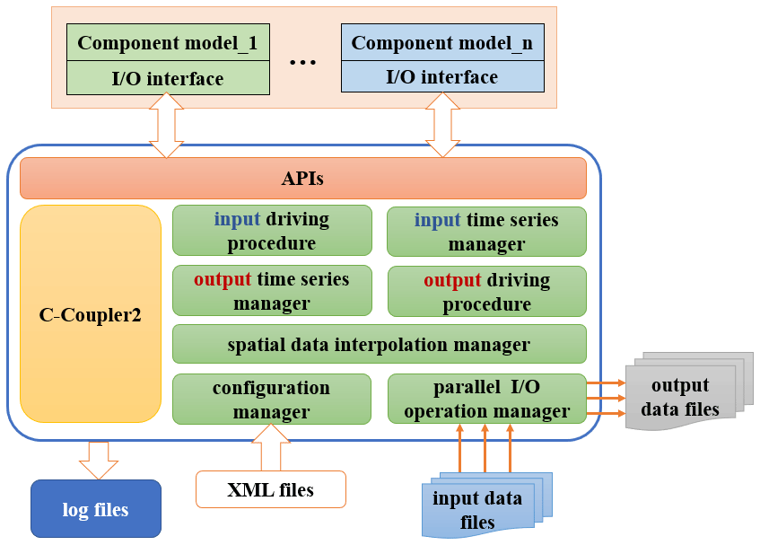
-
The input time series manager handles time series information of data fields in a set of input data files. It enables users to flexibly specify rules for time mapping between data files and models. Given a model time, it determines whether to conduct time interpolation and whether to input the field values at a corresponding time point in a corresponding data file.
-
The output time series manager enables a component model to output model data periodically or irregularly. It determines whether a component model should output model data at the current model time.
-
The spatial data interpolation manager manages the model grid and the file grid for each field. It automatically conducts parallel spatial data interpolation when the model grid and file grid of a field are different.
-
The parallel I/O operation employs parallel I/O supports to write each field into a specific data file and read in data values from a specific data file in parallel.
-
The I/O configuration manager enables users to flexibly specify I/O configurations for a component model via XML formatted configuration files, e.g., configurations for the input/output time series, file grids, and each input/output field.
-
The input driving procedure and output driving procedure organize the procedure for inputting and outputting field values, respectively, based on other modules.
This section introduces details of each module of CIOFC1.0.
3.1 Implementation of the I/O configuration manager
The I/O configuration manager formats a set of XML files for the configuration of the file grids, input/output time series, and each input/output field.
3.1.1 Configuration of file grids
Models generally input forcing fields and output model fields in time integration. Data interpolation is required when a file grid is different from the corresponding model grid. Many models have internal codes of data interpolation for better flexibility of field input and output, especially when unstructured model grids are used. Existing works such as XIOS show the benefit of combining data interpolation and field input/output together in the same framework that can be shared by various models. A challenge arising from such a question is how to specify file grids. The specification via model codes can be inconvenient because users generally must modify and then recompile the model codes when changing file grids in different simulations. XIOS has tried a better solution where a horizontal file grid can be specified via an XML configuration file. We also implemented the I/O configuration manager with XML configurations for file grids.
A challenge here is making the configurations as widely compatible as possible for various grids. C-Coupler can handle various kinds of horizontal grid, support several kinds of vertical coordinates, and represent a 3-D grid in a “2-D + 1-D” or “1-D + 2-D” manner. We therefore design configurations for horizontal grids, vertical coordinates, and 3-D grids.
Configurations for horizontal grids
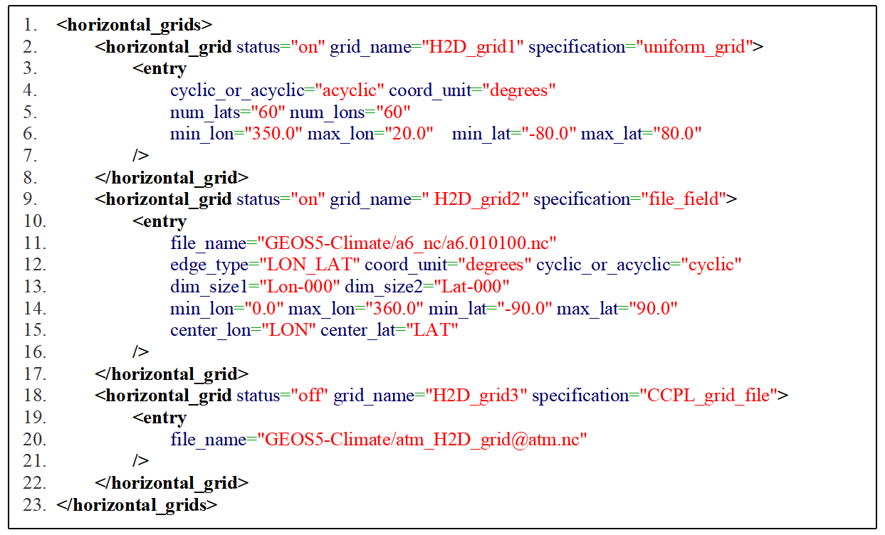
Considering that file grids are usually regular longitude–latitude grids, we simplify the specification of a regular longitude–latitude grid into several parameters in the XML configuration file (e.g., lines 2–8 in Fig. 2): the parameters “min_lon”, “max_lon”, “min_lat”, and “max_lat” specify the domain of the grid, while the parameters “num_lons” and “num_lats” specify the grid size. Thus, the 2-D coordinate values of a longitude–latitude grid can be calculated automatically by CIOFC1.0.
As it is difficult for CIOFC1.0 to automatically calculate coordinate values for an irregular grid, a specification rule is designed to instruct CIOFC1.0 to read in coordinate values from a file (e.g., lines 9–17 in Fig. 2), where the XML attribute “file_name” specifies the file and the attributes “center_lon” and “center_lat” specify the fields of the center coordinate values in the file. The file fields for vertex coordinate values, mask, and area of each grid cell can be further specified via the XML configuration file (not shown in Fig. 2).
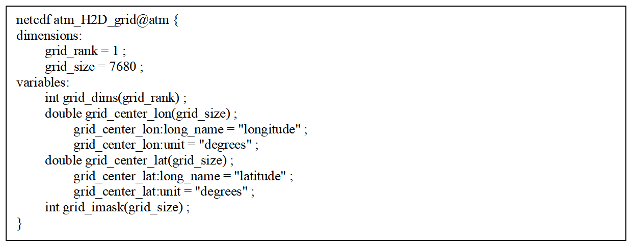
The specification of a file grid can be further simplified into a unique file name (e.g., lines 18–22 in Fig. 2) when it corresponds to a NetCDF file that matches C-Coupler's default grid data file format (e.g., Fig. 3).
In an XML configuration file, users can specify several horizontal grids that are identified by different grid names.
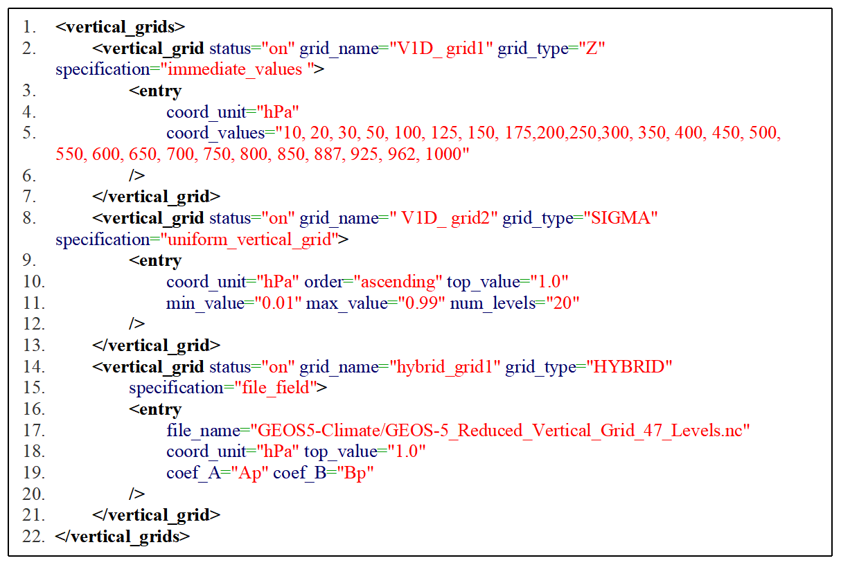
Configurations for vertical coordinates
C-Coupler currently supports three kinds of vertical coordinates: Z, SIGMA (Phillips, 1957), and HYBRID (Simmons and Burridge, 1981) coordinates. We therefore design a specification for each type. (Lines 2–7, 8–13, and 14–21 in Fig. 4 give examples of each of the three types, respectively.) Values of the vertical coordinate can be obtained from fields of a file (lines 14–21 in Fig. 4), specified by an explicit array of values (lines 2 and 7 in Fig. 4), or generated automatically according to the specified boundaries under a descending or ascending order (lines 8–13 in Fig. 4).
In the XML configuration file, users can also specify multiple vertical coordinates that are identified by different grid names.
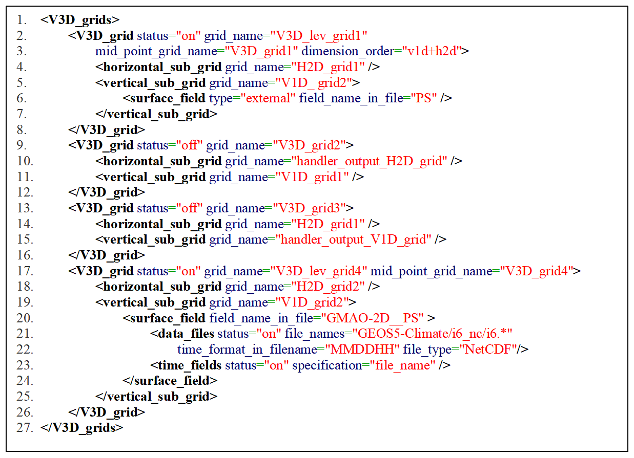
Figure 5An example of specifying 3-D grids in an XML configuration file. The horizontal subgrids “H2D_grid1” and “H2D_grid2” and the vertical subgrids “V1D_grid1” and “V1D_grid2” have already been specified in the same configuration file (Figs. 2 and 4).
Configurations for 3-D grids
In response to the “2-D + 1-D” and “1-D + 2-D” representations of a 3-D grid in C-Coupler, CIOFC1.0 enables users to specify the horizontal and vertical subgrids of a 3-D grid in the XML configuration file (e.g., lines 2–8 and 9–12 in Fig. 5). Given a 3-D grid with a vertical subgrid of SIGMA or HYBRID coordinate, information about the surface field should be specified. A surface field can be specified as a field read from a data file (lines 17–26 in Fig. 5); it can alternatively be specified as a field from the model, meaning that values of the surface field originate from the component model when outputting a field. In a possible special case, users may want a file grid to use the same horizontal or vertical subgrid as the model. A special horizontal grid name “handler_output_H2D_grid” (lines 9–12 in Fig. 5) and a special vertical subgrid name “handler_output_V1D_grid” (lines 13–16 in Fig. 5) are employed for such a case.
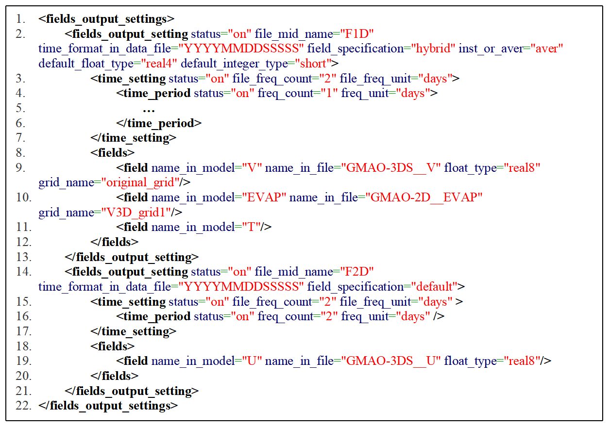
Figure 6An example of configurations for outputting fields in an XML configuration file. The “V3D_grid1” grid has already been specified in line 3 of Fig. 5.
3.1.2 Configurations for outputting fields
Considering that users may want to output different fields with different settings (e.g., different time series, different file grids, and different data types), CIOFC1.0 enables users to specify a specific configuration for a group of fields (e.g., lines 8–12 and 18–20 in Fig. 6). For a field group, users can specify common output settings (line 2 in Fig. 6), e.g., frequency of creating a new file (corresponding to the XML attributes “file_freq_count” and “file_freq_unit”), default data types, output time series (“…” in line 5, which will be further discussed in Sect. 3.4), time format in data files, outputting instantaneous values or time-averaged values, and file grids. A field in a group can also have its own specific settings (line 9 in Fig. 6). Users can make a field use the same name in both the model and data files (line 11 in Fig. 6) or make data files use a new field name (the corresponding XML attribute “name_in_file” is specified; lines 9 and 10 in Fig. 6). As a result, a model can output its fields into multiple files through dividing these fields into multiple field groups.
How to specify the output time series will be further discussed in Sect. 3.2.
3.1.3 Configurations for inputting time series data fields
Considering that the time series fields in data files can be shared by different component models and different simulation settings, the configurations for inputting time series data fields are divided into two parts: information about a time series dataset, and how to bridge a dataset and a component model.
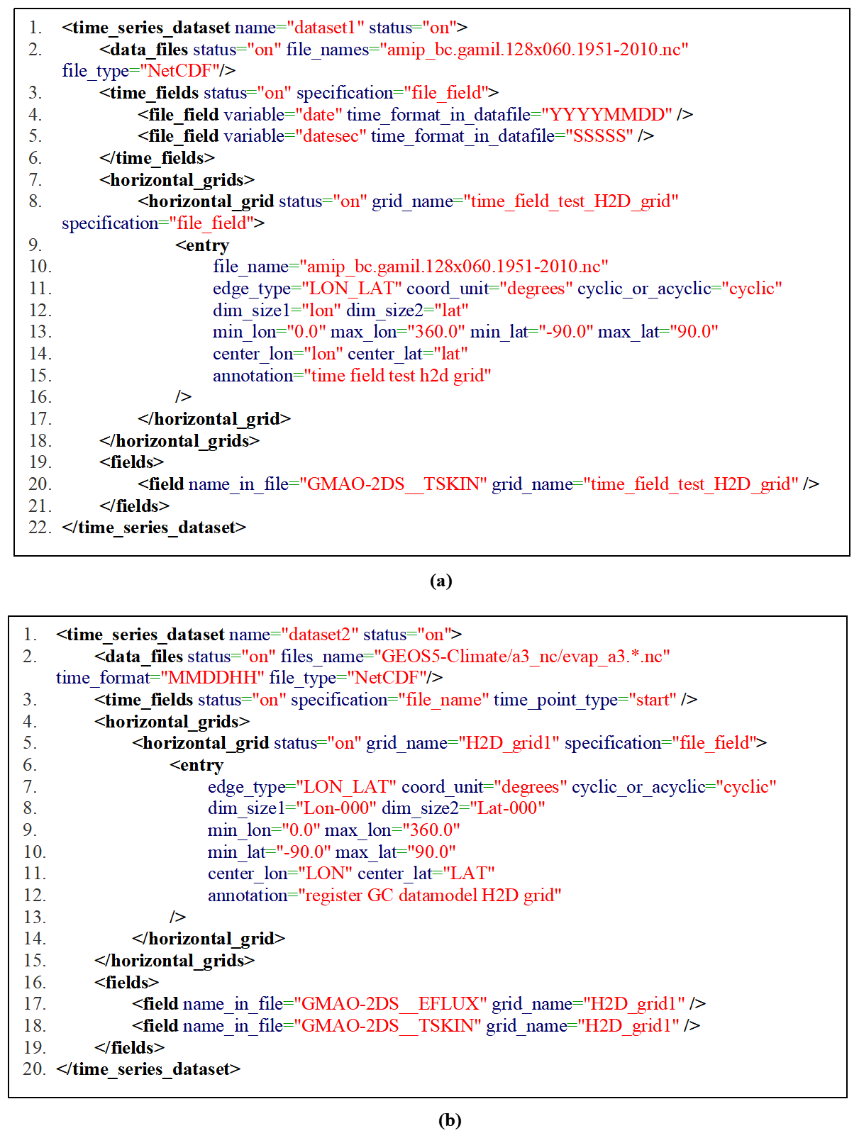
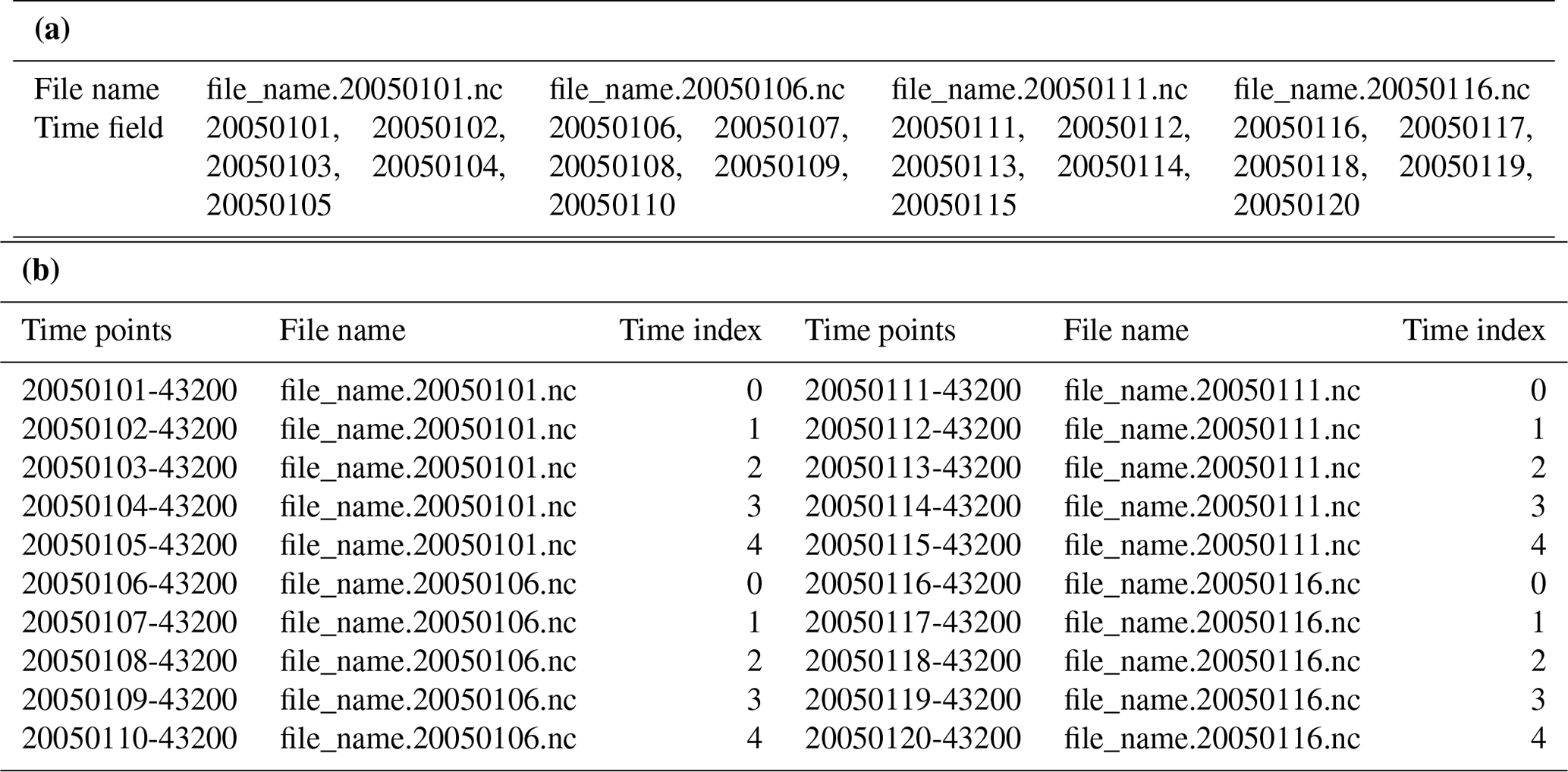
Figure 7Examples of configurations for time series information of input data files: specifying time points through (a) the names of data files and (b) the time fields in data files.
For specifying the data files included in a dataset, CIOFC1.0 enables a dataset to have a unique data file (e.g., line 2 in Fig. 7a) or consist of a group of data files whose names are different only in terms of time (line 2 in Fig. 7b, where the unique character “*” in the common file name will be automatically replaced by the time string under the specified time format when determining the name of each input data file). The time points in a time series can be obtained from the name of the data files (e.g., corresponding to the character “*” in line 2 in Fig. 7b) or from a set of time fields in the data files (lines 3–6 in Fig. 7a) with a specified type of time points (i.e., “start”, “middle”, or “end”; line 3 in Fig. 7b). For example, given a time format “MMDDHH” (representing month, day, and hour), “start”, “middle”, and “end” means the 0th, 1800th, and 3600th second in each hour. The fields provided by a group of data files, as well as the grid of each field, should be listed explicitly (lines 19–21 in Fig. 7a). Each configuration file contains only one dataset with a unique dataset name as the keyword (e.g., the dataset named “dataset1” corresponding to line 1 in Fig. 7a).
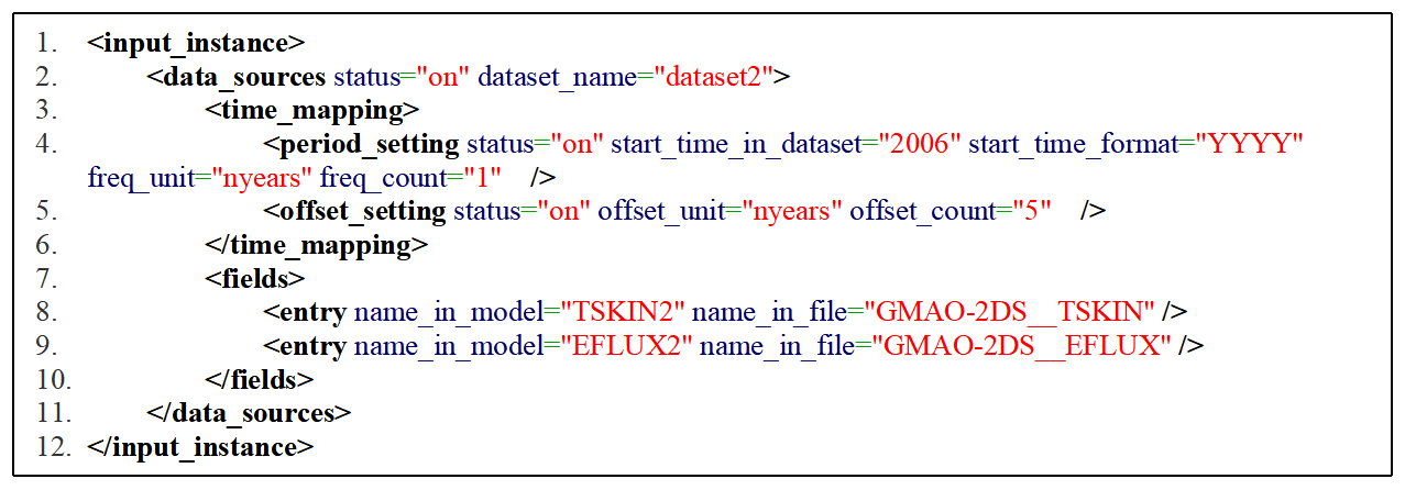
Figure 8An example of configuring an input instance. The dataset “dataset2” corresponds to that specified in Fig. 7b.
A component model can call the corresponding API (Sect. 3.7) to input fields from a time series dataset based on an input instance with a unique name. As the same field may have different names in a dataset and a component model, specification of name mapping for each field is enabled (lines 7–10 in Fig. 8). The time range of a dataset is generally fixed, while users may want flexible use of a dataset in different simulations. For example, a pre-industrial control simulation of a coupled model corresponding to the coupled model intercomparison projects always uses forcing data for the year 1850. Scientists may want to use different time ranges for atmosphere forcing data with the same time range as emissions forcing data in atmospheric chemistry simulations, to study the impact of climate variation on air pollution. We therefore enable users to specify mapping rules between the dataset time and model time (lines 3–6 in Fig. 8), i.e., uses can set a fixed offset between the model time and data time, a fixed period for periodically using time series data, or even a hybrid combination of the two.
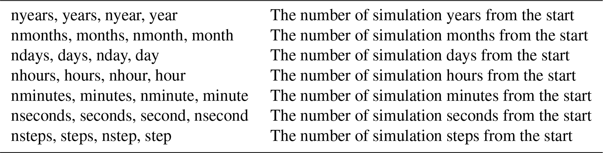
To further improve the commonality in specifying the input time series manager, as well as in the whole CIOFC1.0 system, various time formats, including calendar time formats and simulation time length units (Tables 1 and 2), are supported.
Table 1Examples of the calendar time formats supported in CIOFC1.0.
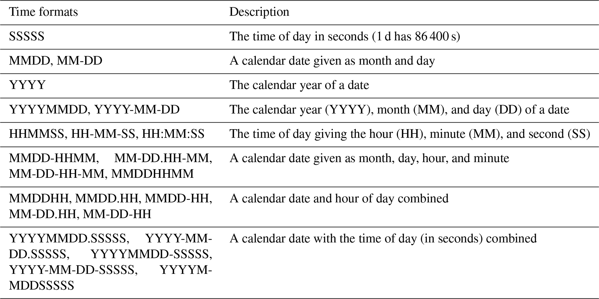
Table 2Examples of the simulation time length units supported in CIOFC1.0.
3.2 Implementation of the spatial data interpolation manager
When a field has a file grid different from its model grid, spatial data interpolation for this field is required. As C-Coupler2.0 already implements horizontal (2-D) interpolation and 3-D interpolation in a “2-D + 1-D” manner, the spatial data interpolation manager directly employs this functionality. (For further details of this functionality, see Liu et al., 2018.) Regarding 2-D interpolation, C-Coupler2.0 can generate online remapping weights based on internal remapping algorithms (i.e., bilinear, first-order conservative, and nearest-neighbor algorithms), or use an off-line remapping weight file generated by other software. Specifically, the spatial data interpolation manager will generate the file grid of each field according to the specifications in the XML configuration file and then determine the remapping weights and conduct data interpolation as required. Different fields with the same model grid and the same file grid can share the same remapping weights.
With such an implementation, CIOFC1.0 enables a model with an unstructured horizontal grid (e.g., a cubed-sphere grid, a non-quadrilateral grid, or even a grid generated by triangulation; Yang et al., 2019) to output fields to a regular longitude–latitude grid in data files. CIOFC1.0 also enables a model with SIGMA or HYBRID vertical coordinates to output fields to Z vertical coordinates in data files, as C-Coupler2.0 supports the dynamic interpolation between two 3-D grids, either of which can calculate variable vertical coordinate values following the change of the corresponding surface field in time integration.
We identified a limitation of C-Coupler2.0 when applying CIOFC1.0 to the atmosphere model MCV that outputs 3-D fields to regular longitude–latitude grids and barometric surfaces in data files. Although C-Coupler2.0 can handle data interpolation between a regular longitude–latitude grid and the cubed-sphere grid used by MCV, it cannot handle vertical interpolation to barometric surfaces, because MCV uses SIGMA vertical coordinates of height but not barometric pressure. We therefore developed a new API CCPL_set_3D_grid_3D_vertical_coord_field and the corresponding functionalities to dynamically use 3-D barometric pressure values diagnostically calculated by MCV during the vertical interpolation to barometric surfaces.
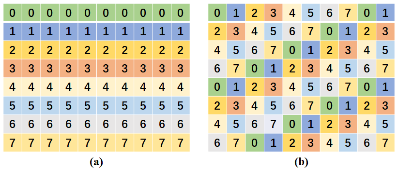
Figure 9An example of two kinds of parallel decomposition: (a) regular 2-D decomposition, with each process associated with one subdomain; and (b) round-robin-based decomposition, which associates each process with multiple subdomains.
3.3 Implementation of parallel I/O
Considering that models for earth system modeling generally access data files in NetCDF format and that C-Coupler implements NetCDF as the default data file format, we use PnetCDF to develop the parallel I/O operation. PnetCDF enables a group of processes to cooperatively output/input multi-dimensional values of a field to/from a data file, where calling the corresponding PnetCDF APIs enables a process to output/input the field values in a subdomain or a subspace specified via the API argument arrays “starts” and “counts”. The subdomains or subspaces associated with each process are generally determined by the parallel decomposition. For example, as determined by the regular 2-D decomposition in Fig. 9a, each process is associated with one subdomain, while the round-robin-based decomposition in Fig. 9b determines that each process is associated with multiple subdomains. To enable a process to output/input the values in multiple subdomains or subspaces, a straightforward implementation is to call the asynchronous PnetCDF APIs (e.g., ncmpi_iput_var* and ncmpi_iget_var*) multiple times before the calling the API ncmpi_wait_all.
Although PnetCDF can rearrange data values in subdomains or subspaces among processes to improve parallel I/O performance (Thakur et al., 1999), existing works such as the PIO library (Dennis et al., 2011) show that model data rearrangement and grouping to fewer I/O processes before using PnetCDF can further improve the I/O performance and introduce low additional maintenance cost. We also prefer such an approach that can further benefit from C-Coupler2.0, especially the functionality of data rearrangement. Specifically, C-Coupler2.0 takes two main steps for data rearrangement: generating a routing network among processes at the initialization stage, and MPI communications following the routing network at each time of data rearrangement. Optimizations of these two steps have been investigated (Yu et al., 2020; Zhang et al., 2016). In the detailed implementation, a group of I/O processes that are a subset of model processes call PnetCDF APIs, and a regular parallel decomposition on all I/O processes (called “I/O decomposition” hereafter) is generated. Such an implementation makes each I/O process associated with a unique subdomain (or subspace) with an averaged number of grid points, and enables C-Coupler2.0 to work for the data rearrangement between model processes and I/O processes.
A parallel I/O operation implements the following steps to output a field:
-
When the I/O decomposition of this field has not been generated, generate the I/O decomposition and the corresponding routing network between model processes and I/O processes.
-
Rearrange the field values from model processes to I/O processes.
-
Call PnetCDF APIs to write field values into a file in parallel.
A parallel I/O operation implements the following steps to input a field:
-
Generate the I/O decomposition and the corresponding routing network when required (the same as the first step for outputting a field).
-
Call PnetCDF APIs to read in field values from a file in parallel.
-
Rearrange the field values from I/O processes to model processes.
The number of I/O processes can affect the efficiency of parallel I/O operation. It is difficult to automatically determine an optimal number of I/O processes, because it depends greatly on the number of model processes and the hardware/system supports in a high-performance computer. Currently, we enable users to specify an upper bound number of I/O processes via a configuration file (the parameter “max_num_pio_proc” in Fig. 10). The actual number of I/O processes of a component model is the lower value between the upper bound number and the number of model processes.
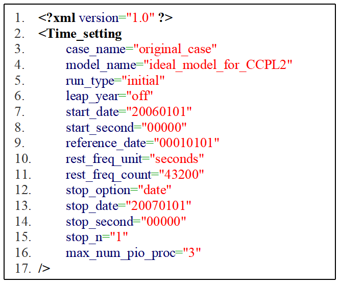
Figure 10An example of specifying the global number of I/O processes in C-Coupler's experiment setup configuration file via the parameter “max_num_pio_proc”.
3.4 Implementation of the output time series manager
C-Coupler2.0 can simply describe the timing of a periodic time series using the period unit and period count. Given a restart timer with unit month and count 5, the model simulation outputs a restart data file every 5 model months. However, time series with irregular patterns have been used in real models but have not previously been supported by C-Coupler2.0. For example, the atmospheric chemistry model GEOS-Chem provides a configuration table (e.g., Fig. 12), which enables users to specify dates in calendar years for outputting model data and to specify independent outputting periods on each date, whereas the weather forecasting model GRAPES mentioned in Sect. 2 generally uses two periods for outputting: every 3 h for the first five model days and every 6 h for the remaining model days.
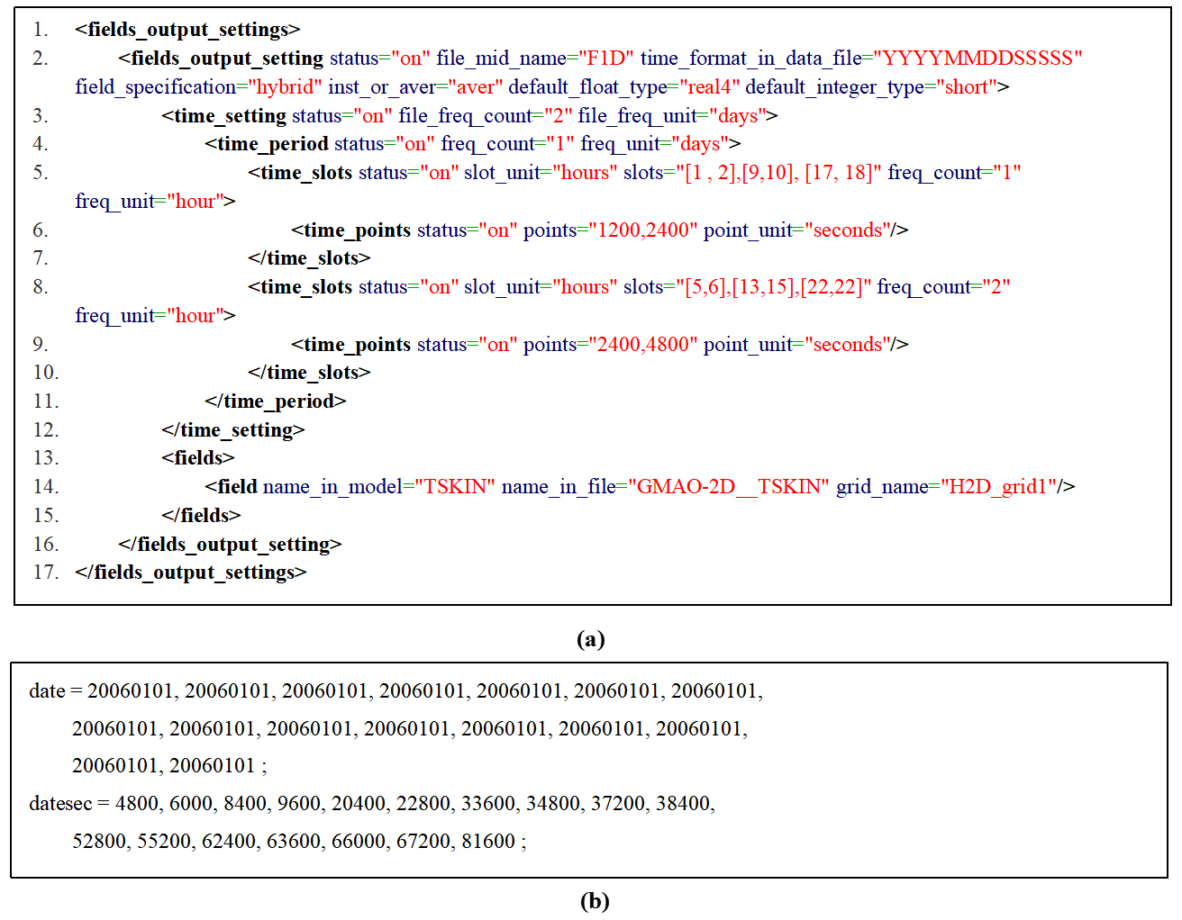
Figure 11An example of specifying an output time series (a) and the corresponding time points in a day (b).
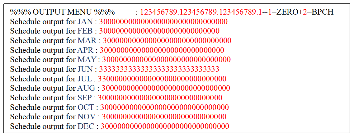
Figure 12An example of output setting of GEOS-Chem. A number “3” means that GEOS-Chem outputs fields every 3 h on the corresponding date of every year, while a number “0” means that GEOS-Chem does not output any field on the corresponding date of every year.
A straightforward solution to describe an irregular time series is to enumerate all time points in the series. We do not recommend this, because it will be inconvenient for long simulations with many time points. A better solution relies on irregular time series generally consisting of several parts with regular periods. The output time series manager should therefore enable users to specify a time series with multiple non-overlapping time slots, most of which have a uniform period. Any time slot with no uniform period should be handled by the output time series manager, enabling users to enumerate all the time points in that slot.
To support various kinds of time series in a convenient manner, the output time series manager employs the terms of period, time slot, and time point, supports flexible combination among them, and enables users to specify an output time series via the XML configuration file. Time slots can be nested in a period, so a period can contain multiple time slots. A period can also be nested in a time slot, which means that a time slot can contain a periodic time series. A period or a time slot can contain multiple time points.
In the example XML specification in Fig. 11a (lines 3–12), the outermost level is a period of every day (line 4). Two groups of time slots are nested in this period (lines 5–10). The time slots of the 1st to 2nd, 9th to 10th, and 17th to 18th hour in the first group nest the same period of every hour (line 5 in Fig. 11a). The time slots of the 5th to 6th, 13th to 14th, and 21st to 22nd hour in the second group nest the same period of every 2 h (line 8 in Fig. 11a). The period in each time slot group further includes time points (lines 6 and 9). This example specification determines a complex irregular time series. (All time points in 1 d are shown in Fig. 11b.)
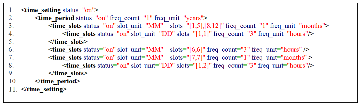
Figure 13An example of the specification of the output time series for GEOS-Chem in CIOFC1.0 corresponding to the specification in Fig. 12.
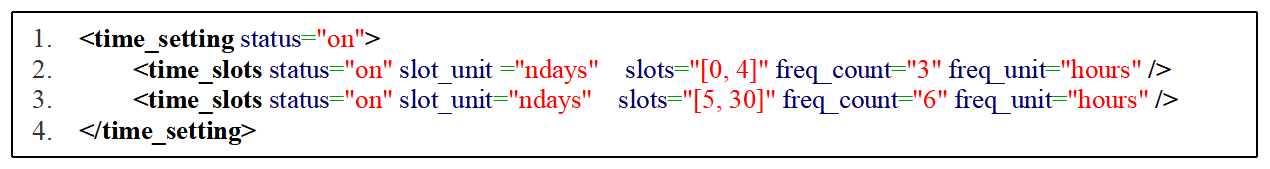
Figure 13 shows the XML specification corresponding to the specific output settings of GEOS-Chem in Fig. 12. The outermost level is the period of every year (line 2 in Fig. 13). There are three groups of time slots nested in this yearly period (lines 3–9). The first group (lines 3–5) means that the model outputs data every 3 h in the first day of each month from January to May and from August to December. The second group (line 6) means that the model outputs data every 3 h in every day of June. The third group (lines 7–9) means that the model outputs data every 3 h in the first and second days of July. Similarly, the output time series of GRAPES mentioned above can be easily specified, as shown in Fig. 14 (lines 1–4), where the XML attribute value “ndays” means the number of model days since the start of the simulation.
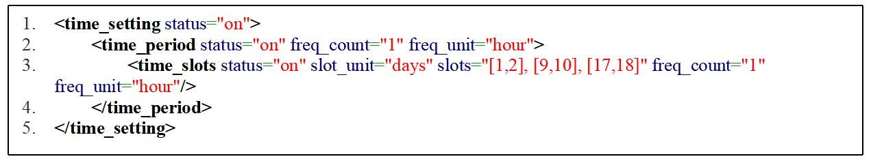
Figure 15An example of an incorrect output time series setting. The frequency unit in the outer level of the specification should be no smaller than that in the inner level.
The output time series manager extends the timer functionality of C-Coupler2.0 – which is only compatible with periodic time series – with a tree of timers to keep the nesting relationship among periods, time slots, and time points. The timer tree of an output time series is initialized when loading the corresponding specifications from the XML configuration file, where the correctness of the nesting relationship will be checked. For example, the specifications in Fig. 15 are incorrect, because the minimum time unit of the period at the outermost level (line 2) is hour, while the minimum time unit of the second level (line 3) is day, which is longer than hour. When the model attempts to output a set of fields, it checks whether the corresponding timer tree is on at the current model time.
Each node in a timer tree corresponds to the timer of a period, a set of time slots, or a set of time points; a node may have multiple children. A recursive procedure is implemented to handle the tree structure. Given a tree node, the procedure first checks whether the corresponding timer is on and then checks each child of the tree node recursively. A tree node is on at the current model time only when its corresponding timer is on, and it has no child or at least one child node is on. A timer of time slots/points is on when the current model time matches one time slot/point.
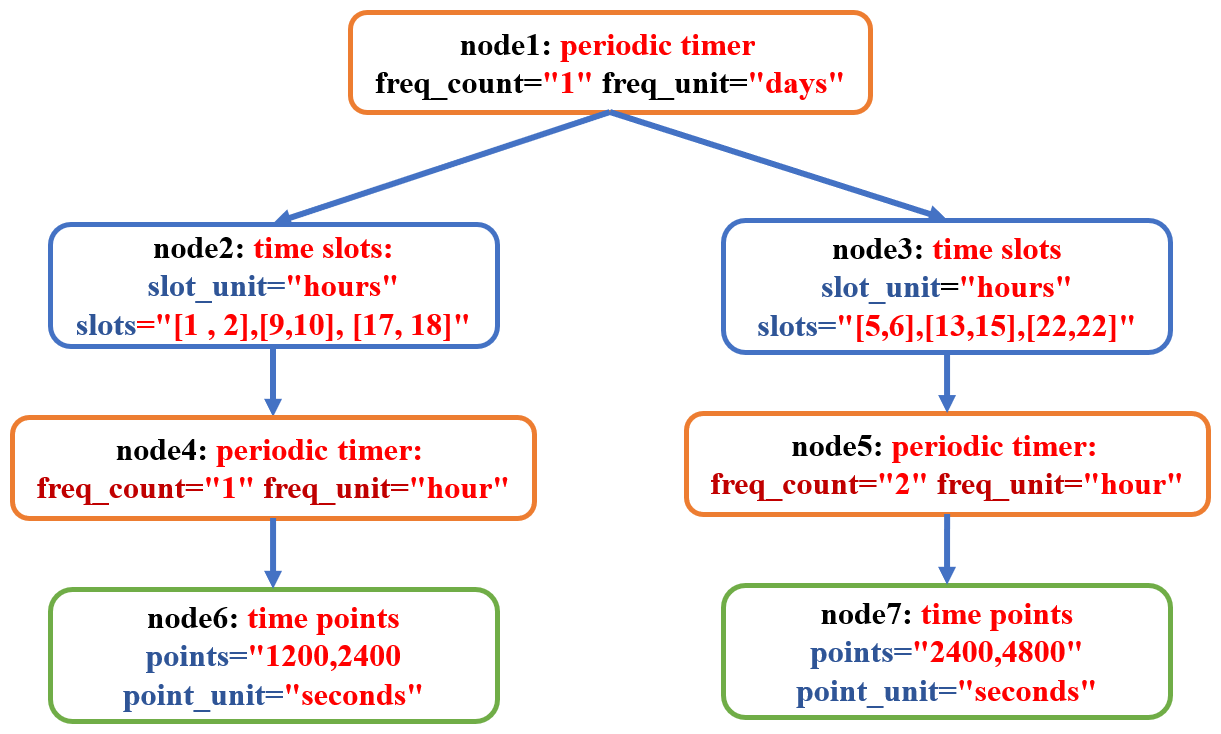
For example, Fig. 16 shows the timer tree corresponding to the output time series specified in Fig. 11a. The root tree node (“node1”) corresponds to the outermost periodic timer. Given a model time of date 20060101 and second 33 600, it matches the period of every day in “node1”, the time slot 9–10 h in “node2”, the period of every hour in “node4”, and the time point of 1200 s in “node6”. So, the timer tree is on at this model time. Given a model time of date 20060101 and second 19 800, it matches the period of every day in “node1”, the time slot 5–6 h in “node3”, and the period of every 2 h in “node7”, but it does not match the time points of 2400 and 4800 s in “node8”. (The time point corresponding to the given model time is 1800 s.) As a result, the timer tree is not on at this model time.
3.5 Implementation of the output driving procedure
The output driving procedure is designed to output model fields with various configurations. Similar to the corresponding implementations in other frameworks, such XIOS, it should combine the attributes (including the field name, data arrays, model grid, and parallel decomposition) of each model field and the corresponding configuration together, so as to conduct data rearrangement and data interpolation. In C-Coupler2.0, a pair of an export interface and an import interface can automatically handle data rearrangement and data interpolation for a set of model fields. To make use of this functionality, the output driving procedure enables a model to apply multiple output handlers each of which corresponds to a set of model fields. Specifically, the API CCPL_register_configurable_output_handler is designed for applying an output handler with complex configurations specified in the XML file, while the API CCPL_register_normal_output_handler is also designed for use with an output handler with simple configurations specified in the argument list but not in the XML file. An output handler can be executed implicitly when the model is advancing model time or executed explicitly through calling the API CCPL_handle_normal_explicit_output.
The implementation of the output driving procedure will be further examined for each API.
3.5.1 Implementation corresponding to the API CCPL_register_configurable_output_handler
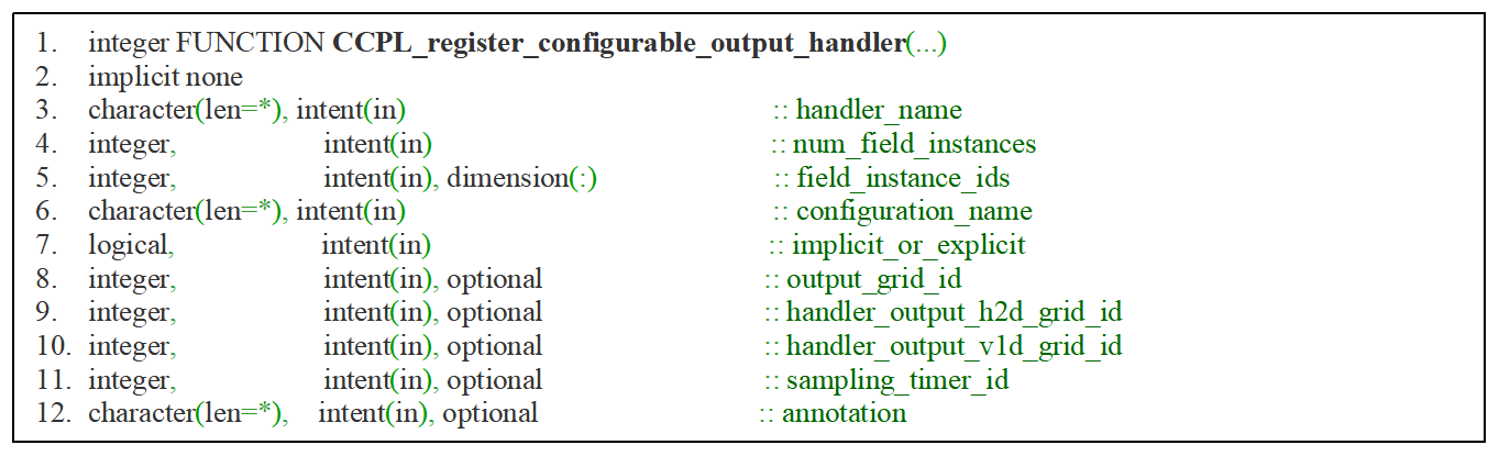
The API CCPL_register_configurable_output_handler provides an argument list for flexibility (Fig. 17). Each output handler has a unique name (corresponding to the argument “handler_name”) and works for a set of field instances (corresponding to the arguments “num_field_instances” and “field_instance_ids”) of the same component model that has already been registered to C-Coupler2.0. Based on the ID of a field instance, the name, data arrays, model grid, and parallel decomposition of the corresponding model field can be obtained. The XML configuration file corresponding to an output handler can be specified via the argument “configuration_name”. Such an implementation enables a component model to use different configurations to output the same group of fields or use the same configuration to output different groups of fields. The execution of an output handler can be either implicit or explicit (corresponding to the argument “implicit_or_explicit”). Users can specify a default file grid (corresponding to the optional argument “output_grid_id”) that has already been registered to C-Coupler2.0, and thus the default file grid will be used for a field when the file grid of this field is not specified in the configuration file. The arguments “handler_output_H2D_grid_id” and “handler_output_V1D_grid_id” correspond to the special subgrids of “handler_output_H2D_grid” and “handler_output_V1D_grid” for configuring 3-D grids in a configuration file (see Sect. 3.1.3). An output handler can be executed at every model time step or under a specified periodic timer (corresponding to the optional argument “sampling_timer_id”). For example, given that a component model with a time step of 60 s outputs time-averaged values of a group of fields every 3 model hours, and that users specify a periodic timer of every hour, the values outputted at the third model hour are averaged from the first 3 model hours, but not from every model step.
The API CCPL_register_configurable_output_handler implements the following main steps to initialize an output handler:
-
Employ the I/O configuration manager to load output configurations from the corresponding XML file. Users will be notified if any error in the XML file is detected.
-
Employ the spatial data interpolation manager to generate all file grids determined by the output configurations.
-
Employ the output time series manager to generate the timer tree of each output time series (called “output timer” hereafter) determined by the output configurations, and generate the periodic timer for creating new data files (called “file timer” hereafter).
-
Determine the output configuration corresponding to each field (e.g., file grid, output time series, file data type, and outputting time-averaged values or instantaneous values).
-
For each file grid, generate a parallel I/O operation as well as the corresponding I/O decomposition, and then allocate the corresponding I/O field instance.
-
Employ the coupling generator of C-Coupler2.0 to generate the coupling procedure from a model field to the corresponding I/O field instance. A coupling procedure can include a group of operations such as data transfer, data interpolation, data type transformation, and data averaging (for further details, see Liu et al., 2018), while the spatial data interpolation manager will generate remapping weights for the data interpolation when necessary. Multiple fields that share the same model grid and the same file grid can share the same I/O field instance and the same coupling procedure, to save memory consumption.
3.5.2 Implementation corresponding to the API CCPL_register_normal_output_handler
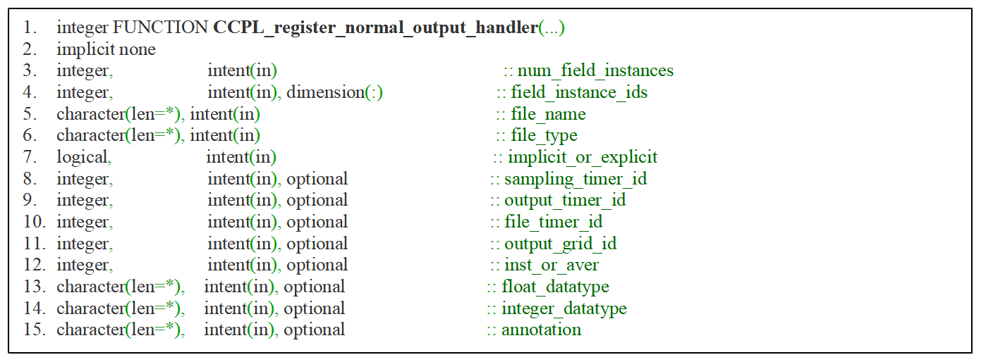
Using the argument list shown in Fig. 18, the API CCPL_register_normal_output_handler works similarly to the API CCPL_register_configurable_output_handler but does not rely on the configurations in the XML file. It can output a group of fields to the same file grid (corresponding to the optional argument “output_grid_id”) that has been previously registered to C-Coupler2.0. Users can specify a periodic timer for outputting fields (corresponding to the optional argument “output_timer_id”) and a periodic timer for generating new data files (corresponding to the optional argument “file_timer_id”). Users can also specify to output time-averaged or instantaneous values of all fields (corresponding to the optional arguments “inst_or_aver”) and specify the data types of fields in data files (corresponding to the optional arguments “float_datatype” and “integer_datatype”).
The API CCPL_register_normal_output_handler uses a flowchart similar to that of the API CCPL_register_configurable_output_handler but without the first and second main steps in Sect. 3.5.1.
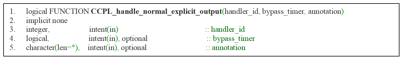
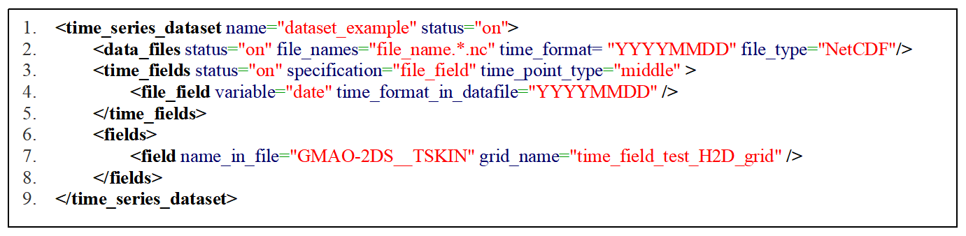
Figure 20An example configuration of a daily input dataset, where the time series is specified via the corresponding time field. The type of time points is set as “middle”, meaning that the time point represents the 43 200th second of a day.
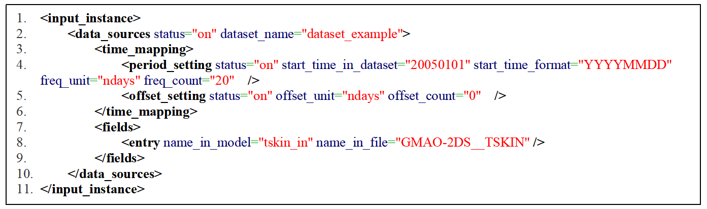
Figure 21An example configuration of the time mapping rule corresponding to the configurations in Fig. 20 and Table 3.
3.5.3 Implementation corresponding to the API CCPL_handle_normal_explicit_output
The API CCPL_handle_normal_explicit_output explicitly executes an output handler that has been applied by calling the API CCPL_register_configurable_output_handler or CCPL_register_normal_output_handler. It is generally called at each model step but actually runs when the sampling timer of the output handler (corresponding to the argument “sampling_timer_id”) is not specified or when the sampling timer is on at the current model time. The current model time is obtained from C-Coupler2.0 implicitly, while C-Coupler2.0 provides APIs for achieving the current model time consistent with the model. When it does run, it first generates a new data file when required and then iterates on each field. For a field, it conducts time averaging if required, conducts data interpolation if required, rearranges the field values on model processes to the I/O processes, and finally outputs the field values on the I/O processes to the data file when the output timer of the field is on. The API CCPL_handle_normal_explicit_output enables users to specify a special argument of “bypass_timer” to disable all timers, which means that the instantaneous values of each field will be outputted to a newly created data file.
The implicit execution of an output handler works similarly to the API CCPL_handle_normal_explicit_output.
3.6 Implementation of the input time series manager
The input time series manager manages the time series information of each input dataset. All time points of an input dataset, as well as the data file and time index corresponding to each time point, are recorded after parsing the corresponding XML configuration file.
Given the current model time, the input time series manager follows the specified mapping rules between the dataset time and the model time, and looks up the corresponding time points of an input dataset, i.e., one time point that matches the current model time or two adjacent time points where the current model time is in the interval between them.
Table 3An example of managing time points in an input dataset with four data files corresponding to the configuration in Fig. 20. Panel (a) displays time fields in each data file. Panel (b) displays the information of time points recorded by CIOFC1.0.
Corresponding to the configuration of a daily input dataset in Fig. 20 (lines 2–5), Table 3a shows the time fields in each of four data files. After parsing this configuration, all daily time points are loaded from these four data files and then extended with a second number (i.e., second 43 200) according to the specified type of the time points (“middle” in Fig. 20), as shown in Table 3b. Lines 3–6 in Fig. 21 specify a time mapping rule hybrid with a period of 20 d and an offset of 5 d. Such a rule determines that the first model day corresponds to the sixth day in the period. Given a simulation starting from a model time of date 20211101 and second 43 200, only one time point (i.e., 2005010643200) in the input dataset corresponds to the start time, while there are two time points (i.e., 2005012043200 and 2005010143200) corresponding to the model time of date 20211115 and second 46 800.
3.7 Implementation of the input driving procedure
To enable a model to iteratively input a group of fields from time series datasets in time integration, the input driving procedure provides an API CCPL_register_input_handler for applying an input handler and provides an API CCPL_execute_input_handler for iteratively executing the input handler. Considering that the initial fields of a model are not generally time series data, an API CCPL_readin_field_from_dataFile reads in values of a field from a specific data file.
Implementation of the input driving procedure is further explored in the following discussion on each API.
3.7.1 Implementation corresponding to the API CCPL_register_input_handler
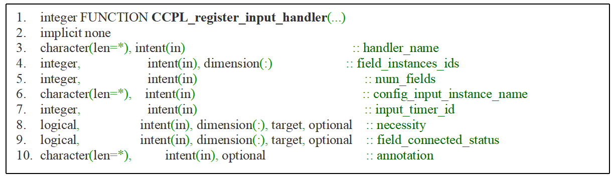
The API CCPL_register_input_handler provides an argument list like that shown in Fig. 22. Similar to the output handler (Sect. 3.5), each input handler also has a unique name (corresponding to the argument “handler_name”) and works for a group of fields (corresponding to the arguments “num_field_instances” and “field_instance_ids”) of the same component model that has already been registered to C-Coupler2.0. The configurations for inputting field values from time series datasets (called “input configurations” hereafter) should be specified (via the argument “config_input_instance_name”). The input handler can also be executed under a specified periodic timer (corresponding to the optional argument “input_timer_id”). Considering that users may require flexibility to change the source of each boundary field of a component model (i.e., the source of a boundary field can be either another component model or a time series dataset) in different simulations of a coupled model, two optional arguments “necessity” and “field_connected_status” are provided. The array “necessity” enables users to specify each field as either necessary or optional (i.e., a necessary field must be input from a dataset and users must specify the input configurations of each necessary field, whereas users can disable the source of an optional field from a dataset through not specifying the input configurations of the field), whereas an element in the array “field_connected_status” notifies whether the input configurations of the corresponding field have been specified. Thus, users can flexibly enable or disable the source of an optional field from a dataset through modifying the corresponding XML configuration file without modifying the model codes.
The API CCPL_register_input_handler implements the following steps to initialize an input handler:
-
Employ the I/O configuration manager to load input configurations from the corresponding XML file. Users will be notified if any error in the XML file is detected.
-
Employ the spatial data interpolation manager to generate all file grids determined by the output configurations.
-
Determine the input configuration corresponding to each field, file grid, data set, data type, etc.
-
For each file grid, generate a parallel I/O operation as well as the corresponding I/O decomposition, and then allocate the corresponding I/O field instance.
-
Employ the input time series manager to manage the time series information of each field and the time mapping rule.
-
Generate the coupling procedure from an I/O field instance to the corresponding model field. This step is similar to the last step of the CCPL_register_configurable_output_handler.
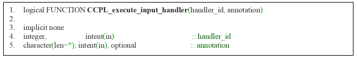
3.7.2 Implementation corresponding to the API CCPL_execute_input_handler
The API CCPL_execute_input_handler executes an input handler that has been applied via an API call of CCPL_register_input_handler. It can be called at any model time and can actually run when the input timer of the input handler is specified and is on at the current model time. When it actually runs, it iterates on each field that can be input from the datasets. For a field, it employs the input time series manager to determine the dataset time points corresponding to the current model time, employs the corresponding parallel I/O operation to read in field values from the dataset corresponding to each time point, rearranges the field values on the I/O processes to model processes, conducts spatial data interpolation operations if required, and finally conducts time interpolation if required.
Here we consider an example with the input configurations in Figs. 20 and 21. When inputting the model field “tskin_in” at the model time of date 20211101 and second 43 200, there is only one dataset time point (i.e., 2005010643200) corresponding to this model time, and thus the field values corresponding to the first time point in the file “file_name.20050106.nc” will be input, and no time interpolation will be conducted. When inputting the model field “tskin_in” at the model time of date 20211101 and second 46 800, there are two dataset time points (i.e., 2005010643200 and 2005010743200) corresponding to this model time, and thus the field values corresponding to the first and second time points in the file “file_ name.20050106.nc” will be inputted, and time interpolation will be conducted.
To reduce I/O overhead, the input driving procedure will cache the field values that have been recently input from datasets. For example, the field values corresponding to the dataset time point 2005010643200 are cached and will not be input again at the model time of date 20211101 and second 46 800.
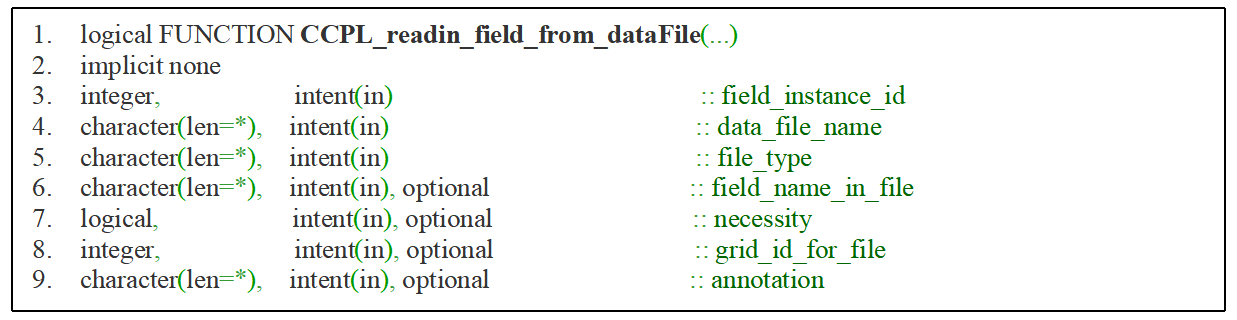
3.7.3 Implementation corresponding to the API CCPL_readin_field_from_dataFile
The API CCPL_readin_field_from_dataFile works for only one model field (corresponding to the argument “field_instance_id” in Fig. 24) and reads in the values of this field from a specific data file (corresponding to the argument “data_file_name”). It enables a field to have a different name (which can be specified via the argument “field_name_in_file”) or a different grid (which can be specified via the argument “grid_id_in_file”) in the data file. Users can further set maximum and minimum boundaries (corresponding to the arguments “value_max_bound” and “value_min_bound”) to prevent input of abnormal values.
The functionality of the API CCPL_readin_field_from_dataFile can be achieved through combining the functionalities of the APIs CCPL_register_input_handler and CCPL_execute_input_handler together for a special case; i.e., only one field to be input without time information.
This section evaluates CIOFC1.0 empirically in terms of functionality and performance. The framework was integrated into real models (GAMIL and MCV); we further developed a test model to enable evaluation of the framework through systematic adjustment of the settings.
All test cases were run on the high-performance computing system (HPCS) of the earth system numerical simulator (http://earthlab.iap.ac.cn/en/, last access: 27 October 2023). The HPCS has approximately 100 000 CPU cores (X86; running at 2.0 GHz) and 80 PB of parallel storage capacity. The HPCS uses a Parastor parallel file system, providing 3–4096 elastic and symmetrical (also supporting asymmetrical architecture) storage nodes. Each computing node includes 64 CPU cores and 256 GB memory, and all of the nodes are connected by a network system with a maximum communication bandwidth of 100 Gbps. All codes are compiled by an Intel Fortran and C++ compiler (version 17.0.5) at the O2 optimization level using an OpenMPI library.
4.1 Test model
Our development of the test model for evaluating CIOFC1.0 focused only on the capabilities for I/O fields, and numerical calculations in real models were neglected. The test model is capable of I/O of 2-D and 3-D fields based on CIOFC1.0 and offers two kinds of horizontal grid (i.e., longitude–latitude and cubed-sphere) and two types of parallel decomposition (i.e., regular 2-D, sequential, and round-robin) for selection. The test model further enables flexible setting of the number of fields, the size of the horizontal grid, the number of vertical levels (the z coordinate is used), and the number of model processes. It also allows to advance integration with a specified time step.
4.2 Functionality of CIOFC1.0
Functionality evaluation considered three categories: correctness of the I/O functionalities, correctness of spatial interpolation, and correctness of I/O time management.
4.2.1 Correctness of the input and output functionalities
We combined the data input and output functionalities when evaluating their correctness, i.e., the test model inputs a set of fields from an existing data file and then outputs these fields into a new data file. We made the test model, the existing data file, and the new data file use the same grids to avoid any spatial data interpolation and associated interpolation error. Therefore, the existing data file and the new data file should be the same when the input and output functionalities are correct. Specifically, we prepared four input data files on cubed-sphere grids under different resolutions and four more on longitude–latitude grids, and finally obtained 16 test cases based on each input data file undergoing the two types of parallel decomposition supported by the test model. The results for each case show the correctness of the I/O functionalities.
CIOFC1.0 enables flexible user-specified setting of the number of I/O processes. A change of the number of I/O processes should not introduce any change to the fields' input or the output data file. Therefore, we further checked the correctness of the I/O functionalities by changing the number of I/O processes. Specifically, we used the 16 test cases above and used three different numbers of I/O processes to run each test case. The results show that CIOFC1.0 produces the same results under different numbers of I/O processes.
4.2.2 Correctness of spatial interpolation
Spatial interpolation is an existing functionality of C-Coupler2.0. As its correctness has already been evaluated (cf. Figs. 11 and 12 in Liu et al., 2018), here we only confirm that it works correctly for CIOFC1.0 if the file grid is different from the model grid in data input or output. Specifically, we reproduced the coupling of the field temperature and zonal wind speed from GAMIL to GEOS-Chem in Liu et al. (2018) and, additionally, made GAMIL output these fields to the grid of GEOS-Chem based on CIOFC1.0. As the fields in the output file were the same as those obtained by GEOS-Chem through coupling, spatial interpolation by CIOFC1.0 was shown to work correctly.
Dynamic 3-D interpolation is a capability that has been further advanced for CIOFC1.0: the new API CCPL_set_3D_grid_3D_vertical_coord_field and the corresponding functionalities enable the 3-D interpolation to use vertical coordinate values dynamically calculated by a model. We further evaluated the correctness of this new enhancement based on MCV – which has an internal code for remapping fields to a regular 3-D grid (consisting of a regular longitude–latitude grid and barometric surfaces) – before outputting the fields. Specifically, we made MCV use CIOFC1.0 to output fields to the same regular 3-D grid. The data files output by MCV internal code and CIOFC1.0 were consistent, demonstrating that the new advancement of dynamic 3-D interpolation has been implemented correctly for CIOFC1.0.
4.2.3 Correctness of I/O time management
Using the test model, we evaluated the correctness of I/O time management for data input and output, respectively. Specifically, we designed a set of different aperiodic output time series. We specified each output time series via the configuration file, ran the test model to get a set of output data files, and then checked whether the time series in these output data files was correct. Next, we made the test model input the aperiodic dataset from each set of output data files and then checked whether time interpolation was conducted correctly (i.e., given each model time, whether CIOFC1.0 used the correct time points in the input time series for time interpolation). The I/O time management functionality was demonstrated to work correctly in all test cases.
4.3 Performance of CIOFC1.0
This subsection evaluates the performance of CIOFC1.0 when inputting and outputting fields based on the test model. A fine-resolution (5 000 000 horizontal grid points and 80 vertical levels) and a coarse-resolution (50 000 grid points and 30 vertical levels) field was used for testing the performance. The data values of each model field are distributed among processes of the test model under a round-robin parallel decomposition. Around 10 000 processor cores ran the test model at fine resolution, and around 500 cores were used for the coarse resolution. Each value in the data files is a single-precision floating point (4 bytes for each value). Each test case was run three times; average performance data are shown here. As the test model is simple and does not do calculation of model fields, we can make the test model output at every time step.
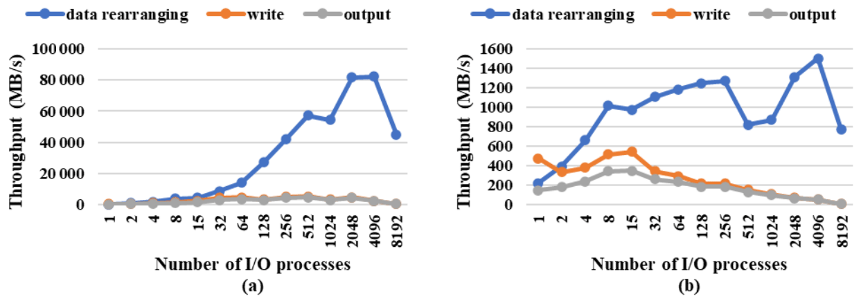
Figure 25Throughput of data rearranging, filesystem writing, and the whole output in (a) a 3-D field and (b) a 2-D field at fine resolution. A total of 10 048 processes were used to run the test model. There is no cost for data interpolation, as fields are on the same longitude–latitude horizontal grid in both the model and data files.
We first evaluated the framework output performance. Figure 25a shows the I/O throughput when outputting a 3-D field (1.6 GB) at the fine resolution as the number of I/O processes increased from 1 to 8192. The whole output throughput took account of the cost of file opening, data rearranging, filesystem writing, and file closing. It did not include the cost of file creation and definition of an I/O decomposition. This is because multiple fields can be written out to the same file, sharing the file creation time and the I/O decomposition time. Both the filesystem writing throughput and the whole output throughput increased quickly as the number of I/O processes increased to 512, with the maximum of 5389 and 4926 MB s−1, respectively. The whole output throughput was over 2500 MB s−1 for 32–4096 I/O processes. The data rearranging was much faster than the filesystem writing in most cases, especially for a large number of I/O processes. This is because the data rearranging is achieved by the data transfer functionality of C-Coupler2.0 that is performed by MPI communications among processes.
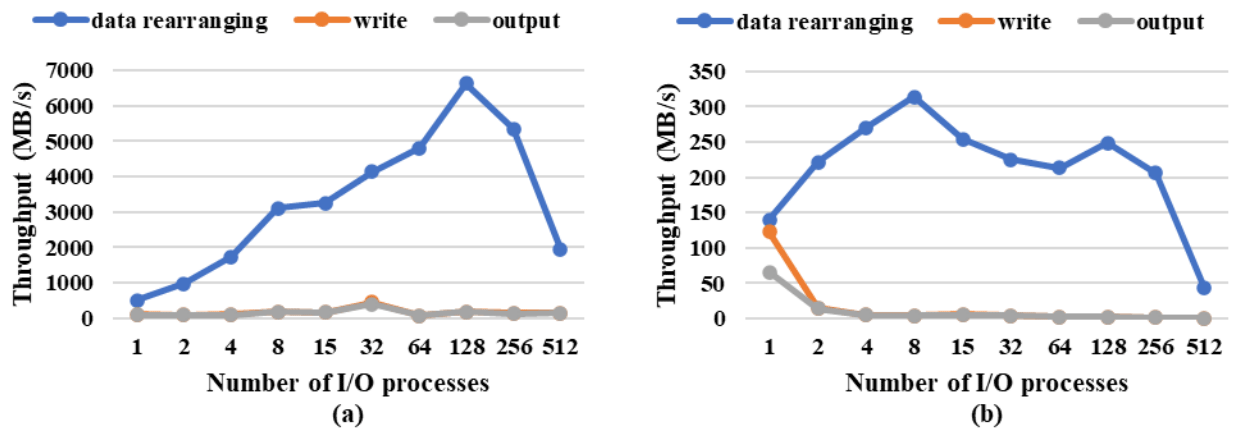
Figure 26As in Fig. 25, but for coarse resolution. A total of 512 processes were used to run the test model.
Figure 25b shows the throughput for outputting a 2-D field (20 MB) at the fine resolution. The maximum output throughput was achieved when using 4–64 I/O processes but was smaller than 400 MB s−1. Figure 26a shows the throughput for outputting a 3-D field (6 MB) at the coarse resolution for increasing the number of I/O processes from 1 to 512; the maximum output throughput was achieved when using 8–32 I/O processes but was smaller than 200 MB s−1. The data rearranging also got much slower but was still faster than the filesystem writing in most cases. Figure 26b shows the maximum output throughput for outputting a 2-D field (200 KB) when using no more than two I/O processes.
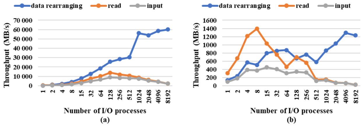
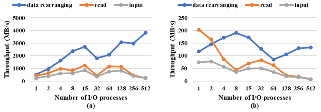
We next evaluated the performance for data input. Figure 27a shows the throughput for inputting a 3-D field at the fine resolution; the maximum throughput was achieved when using 32–1024 I/O processes, with the maximum throughput of 13 946 and 9029 MB s−1 for filesystem read and the whole input at 128 I/O processes. According to Fig. 27b, the maximum input throughput was achieved with 4–32 processes when inputting a 2-D field but was lower than 500 MB s−1. The throughput for inputting a 2-D or 3-D field at the coarse resolution was relatively low especially when using more than 128 I/O processes (Fig. 28). This is because the data size at each CPU core was small and too many I/O system calls take up too much of the total input time.
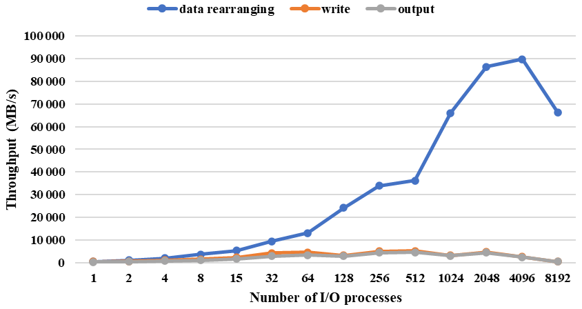
Figure 29The average throughput for outputting 100 3-D fields at fine resolution. A total of 10 048 processes were used to run the test model.
The above results show that although a small field does not benefit from parallel I/O, CIOFC1.0 can accelerate I/O data when the field size in data files is large. For example, compared with serial I/O (corresponding to using one I/O process in Figs. 25–28), throughput can be increased by between 29 and 64 times, respectively, when outputting and inputting a 3-D field at the fine resolution. A model may output a number of fields into the same file. Figure 29 shows the average throughput (cost of file creation was considered) for outputting 100 3-D fields at fine resolution at a time step. It indicates that the performance of outputting one field is applicable to the case of outputting multiple fields continuously.
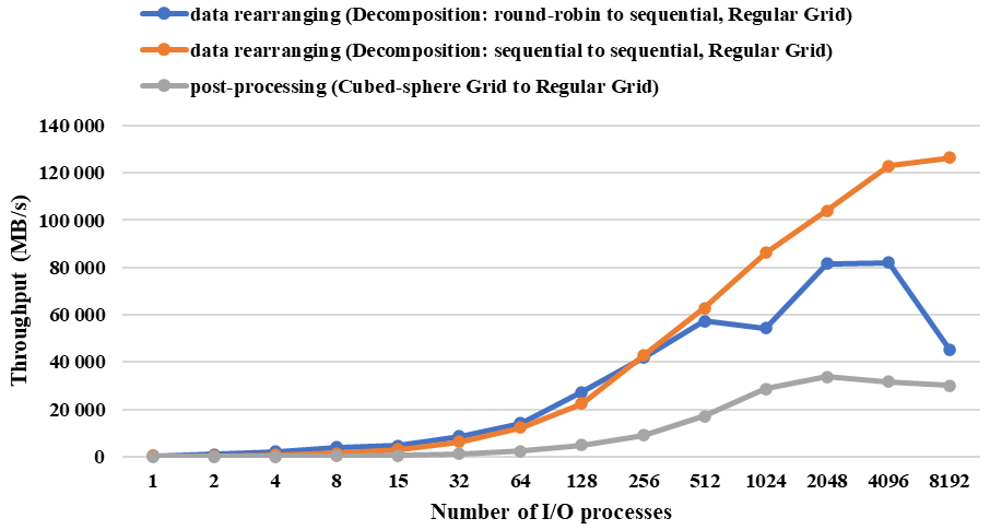
Figure 30The data rearranging throughput when CIOFC1.0 outputs a 3-D field at fine resolution with round-robin decomposition on a regular grid (blue line), with sequential decomposition on a regular grid (orange line), and the post-processing throughput to output a 3-D field at fine resolution on a cubed-sphere model grid to a regular file grid (gray line).
The output/input throughout from Figs. 25 to 29 does not include cost of data interpolation because fields are on the same longitude–latitude horizontal grid in both the model and data files. With regard to outputting a 3-D field under fine resolution, Fig. 30 shows throughput of post-processing with data interpolation and throughput of data rearranging under different parallel decompositions of the field in the model. It is revealed that cost of data rearranging depends on the parallel decomposition, and post-processing with data interpolation introduces higher cost than data rearranging. However, data rearranging and post-processing are much faster than the filesystem writing in most cases.
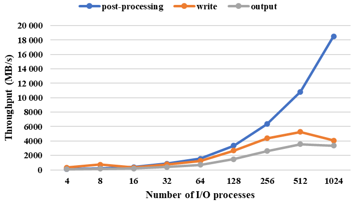
Figure 31The average throughput of post-processing, filesystem writing, and the whole output when outputting 3-D fields for the MCV model under a fine resolution. (The size of a 3-D field in the files is about 1 GB.)
CIOFC1.0 has already been used in a real atmosphere model (i.e., MCV) for accelerating field output. Data interpolation will be performed in field output as the model grid (i.e., a 3-D grid consisting of a cubed-sphere grid and SIGMA-Z vertical coordinate) and the file grid (i.e., a 3-D grid consisting of a longitude–latitude grid and barometric surfaces) are different. Figure 31 shows the average throughput of outputting more than 20 3-D fields into a file under a fine resolution (e.g., 0.125∘ for both the model grid and file grid, 129 vertical levels in the model, and 60 barometric surfaces). Specifically, the maximum throughput is achieved at 512 I/O processes (5281 MB s−1 for filesystem writing and 3550 MB s−1 for whole output). The results indicate that CIOFC1.0 can significantly improve the output for a real model.
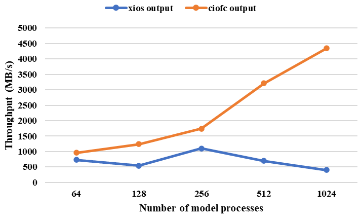
Figure 32The whole throughput of XIOS2.0 and CIOFC1.0 when outputting a 3-D field at fine resolution. Between 64 and 1024 processes were used to run the test model. When running CIOFC1.0, 64, 128, 128, 256, and 256 I/O processes were used, respectively, for the cases with 64, 128, 256, 512, and 1024 model processes.
Figure 32 shows the comparison of throughput between XIOS2.0 and CIOFC1.0. The client mode (synchronous parallel I/O) of XIOS2.0 was used for this comparison. The results show that CIOFC1.0 can achieve higher throughput than XIOS2.0. A possible reason is that CIOFC1.0 enables use of fewer I/O processes than model processes, while all model processes are also I/O processes in XIOS2.0.
In this paper we propose a new common, flexible, and efficient parallel I/O framework for earth system modeling based on C-Coupler2.0. CIOFC1.0 can handle data I/O in parallel and provides a configuration file format that enables users to conveniently change the I/O configurations (e.g., the fields to be output or input, the file grid, and the time series of the data in files). It can automatically interpolate data when required, i.e., it can perform spatial data interpolation when the file grid is different from the model grid, and also time interpolation in data input. It enables a model to output data with an aperiodic time series that can be conveniently specified via the configuration file. Empirical evaluation showed that CIOFC1.0 can accelerate data I/O when the field size is large.
Integration of CIOFC1.0 into a component model generally includes development of the code and configuration files for registering and using the model grids, parallel decompositions, fields, and input/output handlers. A significant advancement achieved by CIOFC1.0 is the cooperative development of an I/O framework and a coupler. CIOFC1.0 benefits greatly from the spatial data interpolation functionality of C-Coupler2.0 and thus can input/output fields with structured or unstructured grids. It needs few new APIs, because it can utilize the existing APIs of C-Coupler2.0 for registering model fields, grids, and parallel decompositions to C-Coupler2.0. As a result, a C-Coupler2.0 user can easily learn how to use CIOFC1.0 or conveniently use a coupler and an I/O framework simultaneously. Conversely, C-Coupler2.0 benefits from CIOFC1.0 to write and read restart data files in parallel. Driven by CIOFC1.0, the dynamic 3-D interpolation of C-Coupler2.0 was further improved. The output time series manager of CIOFC1.0 can help the future development of aperiodic model coupling functionality if required. When CIOFC1.0 output model fields, coordinate fields (e.g., longitude, latitude, vertical levels, and surface field of a 3-D grid) of the corresponding grids will be output. Attributes (e.g., field name, units, and long name) of each field will also be written into an output file. Field attributes can be conveniently specified in the corresponding XML configuration files of CIOFC1.0 and C-Coupler2.0 for different purposes. CIOFC1.0 only supports the classic NetCDF file format (e.g., serial I/O with NetCDF and parallel I/O with PnetCDF) currently. More data file formats such as NetCDF4 and GRIB will be supported in the near future.
CIOFC1.0 is ready for usage by models. Specifically, the atmosphere model MCV, which is under development led by the China Meteorological Administration for the next-generation operational weather forecasting in China, benefits from CIOFC1.0 in several terms, e.g., data interpolation of 3-D fields from the irregular 2-D/3-D model grid to a regular 2-D/3-D file grid, data read/write in parallel, and adaptive input and time interpolation for the time series forcing fields (such as sea surface temperature) during integration. Although the timer tree has not been used at the current development stage of MCV (i.e., MCV currently outputs fields periodically), it will enable MCV to conveniently achieve multiple time segments with different output periods in the future operational applications. We believe that more newly developed models can benefit from CIOFC1.0.
The empirical results in Sect. 4.3 revealed that the number of I/O processes for fastest data I/O highly depends on the field size. A component model generally inputs and outputs 2-D and 3-D fields in simulation, whereas there may be no number of I/O processes that achieves the fastest data input and output for 3-D and 2-D fields simultaneously. For example, at the fine resolution, 512 and 15 I/O processes achieved the fastest data output for 3-D and 2-D fields but did not achieve the fastest input of a 3-D field. As a coupled model can include different component models at different resolutions, and thus different field sizes, different component models may require different settings for the numbers of I/O processes. CIOFC1.0 will become a part of the next generation of C-Coupler, C-Coupler3.0, which will allow users to specify the I/O process numbers (e.g., for data input and output of 2-D and 3-D fields, respectively) separately for each component model. The optimal number of I/O processes may be case dependent in terms of data size of a field, hardware and file system of a parallel storage, structure and performance of the network, usage of a high-performance computer by multiple applications, and so forth. To find a near optimal number of I/O processes, a straightforward solution is to conduct profiling with a number of short simulations under different numbers of I/O processes. Currently, a simple strategy is used in CIOFC1.0 for evenly picking out I/O processes from model processes according to the model process IDs (for example, when picking out 100 I/O processes from 1000 model processes, the model process whose ID is an integral multiple of 10 will become an I/O process). Such a strategy tries to make I/O processes evenly distributed among computing nodes. More strategies may be required in the future when taking into consideration different machine architectures.
Related works have already shown the effectiveness of asynchronous I/O in further reducing the I/O overhead for model simulations (Godoy et al., 2020; Yepes-Arbós et al., 2022; Huang et al., 2014). Currently, CIOFC1.0 does not implement asynchronous I/O. Our future work will seek to incorporate asynchronous I/O in C-Coupler3.0. We will also consider how the various component models in a coupled model cooperatively use the asynchronous I/O functionality.
The source code of CIOFC1.0 can be viewed and run with C-Coupler2.0 and the test model via https://doi.org/10.5281/zenodo.7648563 (Yu et al., 2023). (Please contact us for authorization before using CIOFC1.0 for developing a system.)
XY contributed to the software design, was responsible for code development, software testing, and experimental evaluation of CIOFC1.0, and co-led the writing of the paper. LL initiated this research, was responsible for the motivation and design of CIOFC1.0, supervised XY, and co-led the writing of the paper. CS, ZZ, QJ, BZ, and HY contributed to code development, software testing, and evaluation. BW contributed to the motivation and evaluation. All authors contributed to the improvement of the concepts and content of this work.
The contact author has declared that none of the authors has any competing interests.
Publisher's note: Copernicus Publications remains neutral with regard to jurisdictional claims made in the text, published maps, institutional affiliations, or any other geographical representation in this paper. While Copernicus Publications makes every effort to include appropriate place names, the final responsibility lies with the authors.
This work was jointly supported in part by both, the National Key Research Project of China (grant nos. 2019YFA0606604 and 2017YFC1501903) and the Natural Science Foundation of China (grant no. 42075157).
This research has been jointly supported by both, the National Key Research Project of China (grant nos. 2019YFA0606604 and 2017YFC1501903) and the Natural Science Foundation of China (grant no. 42075157).
This paper was edited by Richard Mills and reviewed by two anonymous referees.
Balaji, V., Anderson, J., Held, I., Winton, M., Durachta, J., Malyshev, S., and Stouffer, R. J.: The Exchange Grid: a mechanism for data exchange between Earth System components on independent grids, in: Lect. Notes. Comput. Sc, Elsevier, 179–186, https://doi.org/10.1016/B978-044452206-1/50021-5, 2006.
Brunet, G., Jones, S., and Ruti, P. M.: Seamless prediction of the Earth System: from minutes to months, Tech. Rep. WWOSC-2014, World Meteorological Organization, 2015.
Chen, C., Li, X., Shen, X., and Xiao, F.: Global shallow water models based on multi-moment constrained finite volume method and three quasi-uniform spherical grids, J. Comput. Phys., 271, 191–223, https://doi.org/10.1016/j.jcp.2013.10.026, 2014.
Craig, A., Valcke, S., and Coquart, L.: Development and performance of a new version of the OASIS coupler, OASIS3-MCT_3.0, Geosci. Model Dev., 10, 3297–3308, https://doi.org/10.5194/gmd-10-3297-2017, 2017.
Craig, A. P., Jacob, R., Kauffman, B., Bettge, T., Larson, J., Ong, E., Ding, C., and He, Y.: CPL6: The new extensible, high performance parallel coupler for the Community Climate System Model, Int. J. High. Perform. C., 19, 309–327, https://doi.org/10.1177/1094342005056117, 2005.
Craig, A. P., Vertenstein, M., and Jacob, R.: A new flexible coupler for earth system modeling developed for CCSM4 and CESM1, Int. J. High. Perform. C., 26, 31–42, https://doi.org/10.1177/1094342011428141, 2012.
Dennis, J., Edwards, J., Loy, R., Jacob, R., Mirin, A., Craig, A., and Vertenstein, M.: An application-level parallel I/O library for Earth system models, Int. J. High Perform. Comput. Appl., 26, 43–53, 2011.
Godoy, W. F., Podhorszki, N., Wang, R., Atkins, C., Eisenhauer, G., Gu, J., Davis, P., Choi, J., Germaschewski, K., and Huck, K.: Adios 2: The adaptable input output system. a framework for high-performance data management, SoftwareX, 12, 100561, https://doi.org/10.1016/j.softx.2020.100561, 2020.
Griffies, S. M.: Elements of the modular ocean model (MOM), GFDL Ocean Group Tech. Rep, 7, 47, 2012.
Hanke, M., Redler, R., Holfeld, T., and Yastremsky, M.: YAC 1.2.0: new aspects for coupling software in Earth system modelling, Geosci. Model Dev., 9, 2755–2769, https://doi.org/10.5194/gmd-9-2755-2016, 2016.
Heinzeller, D., Duda, M. G., and Kunstmann, H.: Towards convection-resolving, global atmospheric simulations with the Model for Prediction Across Scales (MPAS) v3.1: an extreme scaling experiment, Geosci. Model Dev., 9, 77–110, https://doi.org/10.5194/gmd-9-77-2016, 2016.
Huang, X. M., Wang, W. C., Fu, H. H., Yang, G. W., Wang, B., and Zhang, C.: A fast input/output library for high-resolution climate models, Geosci. Model Dev., 7, 93–103, https://doi.org/10.5194/gmd-7-93-2014, 2014.
Jacobsen, D. W., Gunzburger, M., Ringler, T., Burkardt, J., and Peterson, J.: Parallel algorithms for planar and spherical Delaunay construction with an application to centroidal Voronoi tessellations, Geosci. Model Dev., 6, 1353–1365, https://doi.org/10.5194/gmd-6-1353-2013, 2013.
Krishna, J., Wu, D., Kurc, T., Edwards, J., and Hartnett, E.: SCORPIO, GitHub [software], https://github.com/E3SM-Project/scorpio (last access: 30 November 2022), 2020.
Larson, J., Jacob, R., and Ong, E.: The model coupling toolkit: A new Fortran90 toolkit for building multiphysics parallel coupled models, Int. J. High. Perform. C., 19, 277–292, https://doi.org/10.1177/1094342005056115, 2005.
Li, J., Liao, W.-k., Choudhary, A., Ross, R., Thakur, R., Gropp, W., Latham, R., Siegel, A., Gallagher, B., and Zingale, M.: Parallel netCDF: A high-performance scientific I/O interface, SC'03: Proceedings of the 2003 ACM/IEEE Conference on Supercomputing, 39–39, https://doi.org/10.1109/SC.2003.10053, 2003.
Li, L., Lin, P., Yu, Y., Wang, B., Zhou, T., Liu, L., Liu, J., Bao, Q., Xu, S., and Huang, W.: The flexible global ocean-atmosphere-land system model, Grid-point Version 2: FGOALS-g2, Adv. Atmos. Sci., 30, 543–560, https://doi.org/10.1007/s00376-012-2140-6, 2013a.
Li, L., Wang, B., Dong, L., Liu, L., Shen, S., Hu, N., Sun, W., Wang, Y., Huang, W., and Shi, X.: Evaluation of grid-point atmospheric model of IAP LASG version 2 (GAMIL2), Adv. Atmos. Sci., 30, 855–867, https://doi.org/10.1007/s00376-013-2157-5, 2013b.
Li, L., Dong, L., Xie, J., Tang, Y., Xie, F., Guo, Z., Liu, H., Feng, T., Wang, L., and Pu, Y.: The GAMIL3: Model description and evaluation, J. Geophys. Res.-Atmos., 125, e2020JD032574, https://doi.org/10.1029/2020JD032574, 2020a.
Li, L., Yu, Y., Tang, Y., Lin, P., Xie, J., Song, M., Dong, L., Zhou, T., Liu, L., and Wang, L.: The flexible global ocean-atmosphere-land system model grid-point version 3 (fgoals-g3): description and evaluation, J. Adv. Model. Earth. Sy., 12, e2019MS002012, https://doi.org/10.1029/2019MS002012, 2020b.
Li, X., Chen, C., Shen, X., and Xiao, F. A Multimoment Constrained Finite-Volume Model for Nonhydrostatic Atmospheric Dynamics, Mon. Weather Rev., 141, 1216–1240, 2013.
Lin, P., Liu, H., Xue, W., Li, H., Jiang, J., Song, M., Song, Y., Wang, F., and Zhang, M.: A coupled experiment with LICOM2 as the ocean component of CESM1, J. Meteorol. Res-prc., 30, 76–92, https://doi.org/10.1007/s13351-015-5045-3, 2016.
Lin, Y., Huang, X., Liang, Y., Qin, Y., Xu, S., Huang, W., Xu, F., Liu, L., Wang, Y., and Peng, Y.: Community Integrated Earth System Model (CIESM): Description and Evaluation, J. Adv. Model. Earth. Sy, 12, e2019MS002036, https://doi.org/10.1029/2019MS002036, 2020.
Liu, H., Lin, P., Yu, Y., and Zhang, X.: The baseline evaluation of LASG/IAP climate system ocean model (LICOM) version 2, Acta. Meteorol. Sin., 26, 318–329, https://doi.org/10.1007/s13351-012-0305-y, 2012.
Liu, L., Yang, G., Wang, B., Zhang, C., Li, R., Zhang, Z., Ji, Y., and Wang, L.: C-Coupler1: a Chinese community coupler for Earth system modeling, Geosci. Model Dev., 7, 2281–2302, https://doi.org/10.5194/gmd-7-2281-2014, 2014.
Liu, L., Zhang, C., Li, R., Wang, B., and Yang, G.: C-Coupler2: a flexible and user-friendly community coupler for model coupling and nesting, Geosci. Model Dev., 11, 3557–3586, https://doi.org/10.5194/gmd-11-3557-2018, 2018.
Long, M. S., Yantosca, R., Nielsen, J. E., Keller, C. A., da Silva, A., Sulprizio, M. P., Pawson, S., and Jacob, D. J.: Development of a grid-independent GEOS-Chem chemical transport model (v9-02) as an atmospheric chemistry module for Earth system models, Geosci. Model Dev., 8, 595–602, https://doi.org/10.5194/gmd-8-595-2015, 2015.
Palmer, B., Koontz, A., Schuchardt, K., Heikes, R., and Randall, D.: Efficient data IO for a parallel global cloud resolving model, Environ. Modell. Softw., 26, 1725–1735, https://doi.org/10.1016/j.envsoft.2011.08.007, 2011.
Phillips, N. A.: A coordinate system having some special advantages for numerical forecasting, J. Meteor., 14, 184–185, 1957.
Putman, W. M. and Lin, S.-J.: Finite-volume transport on various cubed-sphere grids, J. Comput. Phys., 227, 55–78, https://doi.org/10.1016/j.jcp.2007.07.022, 2007.
Redler, R., Valcke, S., and Ritzdorf, H.: OASIS4 – a coupling software for next generation earth system modelling, Geosci. Model Dev., 3, 87–104, https://doi.org/10.5194/gmd-3-87-2010, 2010.
Ren, S., Liang, X., Sun, Q., Yu, H., Tremblay, L. B., Lin, B., Mai, X., Zhao, F., Li, M., Liu, N., Chen, Z., and Zhang, Y.: A fully coupled Arctic sea-ice–ocean–atmosphere model (ArcIOAM v1.0) based on C-Coupler2: model description and preliminary results, Geosci. Model Dev., 14, 1101–1124, https://doi.org/10.5194/gmd-14-1101-2021, 2021.
Shi, R., Xu, F., Liu, L., Fan, Z., Yu, H., Li, H., Li, X., and Zhang, Y.: The effects of ocean surface waves on global intraseasonal prediction: case studies with a coupled CFSv2.0–WW3 system, Geosci. Model Dev., 15, 2345–2363, https://doi.org/10.5194/gmd-15-2345-2022, 2022.
Simmons, A. J. and Burridge, D. M..: An Energy and Angular Momentum Conserving Finite-difference Scheme and Hybrid Vertical Coordinates, Mon. Weather Rev., 1–9, 758–766, 1981.
Smith, R., Jones, P., Briegleb, B., Bryan, F., Danabasoglu, G., Dennis, J., Dukowicz, J., Eden, C., Fox-Kemper, B., and Gent, P.: The parallel ocean program (POP) reference manual ocean component of the community climate system model (CCSM) and community earth system model (CESM), LAUR-01853, 141, 1–140, 2010.
Tang, J., Chen, C., Shen, X., Xiao, F., and Li, X.: A positivity-preserving conservative Semi-Lagrangian Multi-moment Global Transport Model on the Cubed Sphere, Adv. Atmos. Sci., 38, 1460–1473, https://doi.org/10.1007/s00376-021-0393-7, 2021.
Thakur, R., Gropp, W., and Lusk, E.: Data sieving and collective I/O in ROMIO, Proceedings. Frontiers' 99. Seventh Symposium on the Frontiers of Massively Parallel Computation, 182–189, https://doi.org/10.1109/FMPC.1999.750599, 1999.
Valcke, S.: The OASIS3 coupler: a European climate modelling community software, Geosci. Model Dev., 6, 373–388, https://doi.org/10.5194/gmd-6-373-2013, 2013.
Valcke, S., Balaji, V., Craig, A., DeLuca, C., Dunlap, R., Ford, R. W., Jacob, R., Larson, J., O'Kuinghttons, R., Riley, G. D., and Vertenstein, M.: Coupling technologies for Earth System Modelling, Geosci. Model Dev., 5, 1589–1596, https://doi.org/10.5194/gmd-5-1589-2012, 2012.
Wang, G., Zhao, B., Qiao, F., and Zhao, C.: Rapid intensification of Super Typhoon Haiyan: the important role of a warm-core ocean eddy, Ocean. Dynam., 68, 1649–1661, https://doi.org/10.1007/s10236-018-1217-x, 2018.
Yang, H., Liu, L., Zhang, C., Li, R., Sun, C., Yu, X., Yu, H., Zhang, Z., and Wang, B.: PatCC1: an efficient parallel triangulation algorithm for spherical and planar grids with commonality and parallel consistency, Geosci. Model Dev., 12, 3311–3328, https://doi.org/10.5194/gmd-12-3311-2019, 2019.
Yepes-Arbós, X., Acosta, M. C., van den Oord, G., and Carver, G.: Computational aspects and performance evaluation of the IFS-XIOS integration, European Centre for Medium Range Weather Forecasts, https://doi.org/10.21957/ggapxuny0, 2018.
Yepes-Arbós, X., van den Oord, G., Acosta, M. C., and Carver, G. D.: Evaluation and optimisation of the I/O scalability for the next generation of Earth system models: IFS CY43R3 and XIOS 2.0 integration as a case study, Geosci. Model Dev., 15, 379–394, https://doi.org/10.5194/gmd-15-379-2022, 2022.
Yu, H., Liu, L., Sun, C., Li, R., Yu, X., Zhang, C., Zhang, Z., and Wang, B.: DiRong1.0: a distributed implementation for improving routing network generation in model coupling, Geosci. Model Dev., 13, 6253–6263, https://doi.org/10.5194/gmd-13-6253-2020, 2020.
Yu, X., Liu, L., Sun, C., Jiang, Q., Zhao, B., Zhang, Z., Yu, H., and Wang, B.: CIOFC1.0: a Common Parallel Input/Output Framework Based on C-Coupler2.0, Zenodo [code], https://doi.org/10.5281/zenodo.7648563, 2023.
Zhang, C., Liu, L., Yang, G., Li, R., and Wang, B.: A new adaptive data transfer library for model coupling, Geosci. Model Dev., 9, 2099–2113, https://doi.org/10.5194/gmd-9-2099-2016, 2016.
Zhang, R. and Shen, X.: On the development of the GRAPES – A new generation of the national operational NWP system in China, Chinese Sci. B., 53, 3429–3432, 2008.
Zhao, B., Qiao, F., Cavaleri, L., Wang, G., Bertotti, L., and Liu, L.: Sensitivity of typhoon modeling to surface waves and rainfall, J. Geophys. Res.-Oceans, 122, 1702–1723, https://doi.org/10.1002/2016JC012262, 2017.
Zou, Y., Xue, W., and Liu, S.: A case study of large-scale parallel I/O analysis and optimization for numerical weather prediction system, Future Gener. Comp. Sy., 37, 378–389, https://doi.org/10.1016/j.future.2013.12.039, 2014.