Rapid Adaptive Optimization Model for Atmospheric Chemistry (ROMAC) v1.0

The Rapid Adaptive Optimization Model for Atmospheric Chemistry (ROMAC) is a flexible and computationally efficient photochemical box model. Its unique adaptive dynamic optimization module allows for the dynamic and rapid estimation of the impact of chemical and physical processes on pollutant concentration. ROMAC outperforms traditional box models in evaluating the influence of physical processes on pollutant concentrations. Its ability to quantify the effects of chemical and physical processes on pollutant concentrations has been confirmed through chamber and field observation cases. Since the development of a variable-step and variable-order numerical solver that eliminates the need for Jacobian matrix processing, the computational efficiency of ROMAC has seen a marked improvement with only a marginal increase in error. Specifically, the computational efficiency has improved by 96 % when compared to several established box models, such as F0AM and AtChem. Moreover, the solver maintains a discrepancy of less than 0.1 % when its results are compared with those obtained from a high-precision solver in AtChem.

1 Introduction

Numerical models are effective tools of atmospheric chemistry studies. The 0-dimensional (0-D) box model has been widely used in previous studies to investigate the relationship between secondary pollutants and precursors (Decker et al., 2021, 2019; Ling et al., 2017; Wang et al., 2017; He et al., 2019). The box model can be used as a ground Lagrangian trajectories model to study the influence of the regional transport of precursors on the formation of secondary pollutants (Cheng et al., 2010; Wang et al., 2019). In addition, the box model is also a powerful tool in environmental chamber studies (Chen et al., 2015; Novelli et al., 2018). Several box models have been developed and applied in previous studies, such as AtChem (Sommariva et al., 2020), Chemistry As A Box Model Application (CAABA/MECCA) (Sander et al., 2011, 2019), Framework for 0-D Atmospheric Modeling (F0AM) (Wolfe et al., 2016), PyCHAM (O'Meara et al., 2021), JlBox (Huang and Topping, 2021) and Photochemical Box Model incorporating the Master Chemical Mechanism (PBM-MCM) (Wang et al., 2018).

Since the processes of vertical and horizontal transmission are ignored, the simulation speed of the 0-D box model is higher than that of the 3-D air quality model. This allows box models to use more comprehensive chemical mechanisms and to focus on the analysis of chemical processes. For instance, the utilization of 0-D models in coupling with near-explicit chemical mechanisms can offer a comprehensive understanding of photochemical processes (Y. Wang et al., 2023). However, it is important to consider the impact of physical transport on long-lived species, such as its effect on O₃ concentration (Li et al., 2021; Liu et al., 2022). The 0-D model, which lacks a 3-D structure, is unable to directly estimate the impact of physical processes (e.g., vertical and horizontal transport) on pollutant concentrations. Therefore, it is necessary to find a proper scheme to estimate the physical process for these models. Furthermore, as the atmospheric chemistry mechanism continues to develop, the number of chemical reactions involved gradually increases. Consequently, when using a chemical mechanism with massive reactions, the process of obtaining a chemical solution in a 0-D box model also becomes time-consuming. For example, the Master Chemical Mechanism (MCM v3.3.1) contains about 5900 species (Jenkin et al., 2015), and the size of the Jacobian matrix is close to 5900×5900, which requires a large number of matrix calculations in the process of solving with the implicit solver. Therefore, it is necessary to develop a computationally efficient model for chemical mechanisms. Most of box models rely on third-party tools for differential equation solving. Several multistep or multistage approaches are commonly used by these chemical solvers, such as ROSENBROCK, BDF, LSODE, GEAR, SMVGEAR, etc. (Verwer et al., 1996; Aro, 1996a; Sandu et al., 1997a, b). Although these third-party solving tools have good accuracy and stability, the solving process requires a lot of computing resources, which significantly reduces the computational efficiency.

The simplified chemical mechanism can effectively improve the solution efficiency of chemical processes, such as SAPRC07 (Carter, 2010), CB6 (Yarwood, 2010), MOZART (Emmons et al., 2010) and the Mainz Organic Mechanism (MOM) (Sander et al., 2019). The MCM mechanism also has a simplified version (https://mcm.york.ac.uk/CRI, last access: 21 October 2023), which can improve the computational efficiency. General methods for reduction (Young and Boris (1977); Djouad and Sportisse, 2002) and their on-line implementations (Sander et al., 2019; Shen et al., 2022; Lin et al., 2023) have been developed. These simplified mechanisms generally have a focus on getting particular parts of chemistry. As a result, the simulation results for certain species may diverge from those obtained using near-explicit chemical mechanisms, particularly concerning radicals (e.g., OH, HO₂, RO₂) and the concentrations of secondary pollutants (Ying and Li, 2011; Jimenez, 2003). The adoption of near-explicit chemical mechanisms enables a more detailed representation of the intricate process of photochemical reactions. Consequently, the simplified mechanism cannot adequately replace the role of the near-explicit mechanism. To improve efficiency, another approach is to improve the computational efficiency of differential equation solver programs, such as using GPU acceleration (Alvanos and Christoudias, 2017) or using the quasi-Newton method (Esentürk et al., 2018). These methods can effectively shorten the running time of the program, but still need to consume a lot of memory and CPU (or GPU) resources when processing the Jacobian matrix. There are alternative solution methods that do not need to store and update the Jacobian matrix, such as quasi-steady-state approximation (QSSA), multistep explicit and semi-implicit methods (Mott et al., 2000; Young and Boris, 1977). But these methods usually do not conserve mass (Cariolle et al., 2017). In addition, there are also fully implicit methods that do not need to deal with the Jacobian matrix, such as the Euler backward iterative (EBI) method (Hertel et al., 1993). However, the EBI solver has a large truncation error because it is only first-order accurate. Another stiff ordinary differential equations (ODEs) preconditioner method based on Newton linearization also simplifies the matrix operations during the solution (Aro, 1996a). But these algorithms may fail to converge when the Jacobian matrix is significantly off-diagonally dominant (Aro, 1996b). Hence, with the increasing complexity and scale of chemical mechanism systems, it is still a challenge to make these solving algorithms converge stably.

The Rapid Adaptive Optimization Model for Atmospheric Chemistry (ROMAC) is a computationally efficient photochemical box model. To enhance its computational efficiency, a variable-step and variable-order (VSVOR) solver without Jacobian matrix processing was developed for ROMAC. This distinctive solver offers superior computational efficiency in handling atmospheric chemical mechanisms by eliminating the need for third-party libraries for numerical solving. By utilizing the VSVOR solver, ROMAC provides users with the flexibility to dynamically optimize the influence of physical processes on pollutant concentration, which is difficult to achieve in the traditional box model with oversimplified physical modules. Therefore, ROMAC will be computationally efficient and outperform the traditional box models in evaluating the impact of physical processes on pollutant concentrations.

2 Description of ROMAC

ROMAC is a 0-D model focused on the simulation of atmospheric chemical kinetics problems. It was developed to provide users with a flexible and efficient computational tool. The core modules of ROMAC were developed in Fortran, and the data pre-processing and post-processing modules were developed in Python, which can keep the model running efficiently and provide users with flexible processing tools. In ROMAC, the changes in concentration of a species can mathematically be represented as Eq. (1):

$$\begin{array}{}\text{(1)}& \begin{array}{rl}{\displaystyle \frac{\mathrm{d}c}{\mathrm{d}t}}& ={\left[{\displaystyle \frac{\mathrm{d}c}{\mathrm{d}t}}\right]}_{\mathrm{chem}}+{\left[{\displaystyle \frac{\mathrm{d}c}{\mathrm{d}t}}\right]}_{\mathrm{emis}}+{\left[{\displaystyle \frac{\mathrm{d}c}{\mathrm{d}t}}\right]}_{\mathrm{dry}}\\ & +{\left[{\displaystyle \frac{\mathrm{d}c}{\mathrm{d}t}}\right]}_{\mathrm{dilu}}+{\left[{\displaystyle \frac{\mathrm{d}c}{\mathrm{d}t}}\right]}_{\mathrm{others},}\end{array}\end{array}$$

where ${\left[\frac{\mathrm{d}c}{\mathrm{d}t}\right]}_{\mathrm{chem}}$ represents the changes due to chemical reactions; ${\left[\frac{\mathrm{d}c}{\mathrm{d}t}\right]}_{\mathrm{emis}}$ represents the emission rate for the species; ${\left[\frac{\mathrm{d}c}{\mathrm{d}t}\right]}_{\mathrm{dry}}$ and ${\left[\frac{\mathrm{d}c}{\mathrm{d}t}\right]}_{\mathrm{dilu}}$ represent the dry deposition and dilution, respectively. For dry deposition, ROMAC uses the maximum dry deposition velocity (cm s⁻¹) calculated by Zhang et al. (2003) to estimate the dry deposition process of the species, and users can also customize this value. The dry deposition process is added to the model in the form of first-order kinetics, and the kinetic constant is calculated by the dry deposition velocity and the preset boundary layer height (cm). Similar to other models (Wolfe et al., 2016; Sommariva et al., 2020), ROMAC uses first-order kinetics to calculate the dilution process, and users can customize the constants of the dilution process. Note that the current version of ROMAC does not feature a dedicated input function for wet deposition. Instead, ROMAC allows users to set a custom rate term, ${\left[\frac{\mathrm{d}c}{\mathrm{d}t}\right]}_{\mathrm{others}}$, which can be employed to account for wet deposition. If wet deposition is important for the simulation case, especially concerning the chemical mechanism of hydrophilic components like sulfate, it is suggested that the user incorporates it into ${\left[\frac{\mathrm{d}c}{\mathrm{d}t}\right]}_{\mathrm{others}}$. Moreover, users have the flexibility to add additional change rates as needed, such as the gas-wall partitioning in the chamber studies or the external transport (e.g., vertical and horizontal transport) in field observations. It is not a difficult task to incorporate new rates of change into ${\left[\frac{\mathrm{d}c}{\mathrm{d}t}\right]}_{\mathrm{others}}$ within the ROMAC framework.

The subsequent sections offer a comprehensive overview of the ROMAC features. Furthermore, to facilitate reference, all the parameters employed in this paper are catalogued in Appendix B.

2.1 High-efficiency solver for atmospheric chemical kinetic equations

Unlike many existing models, ROMAC distinguishes itself by not relying on third-party libraries for numerical solving. Instead, ROMAC employs its own computationally efficient variable-step and variable-order numerical solver named “VSVOR.” This solver is engineered to enhance computational efficiency while accommodating the universal attributes of atmospheric chemical mechanisms. It approaches all differential equations uniformly, eliminating the need for customized solution schemes tailored to specific chemical mechanisms. Therefore, the VSVOR solver offers a universal and versatile method for chemical solving. The VSVOR solver has a control on the truncation error of integration according to the relative tolerance (rtol) and the absolute tolerance (atol) specified by the user. The proposed solver offers an algorithm that strikes a balance between efficiency and accuracy. Most of the time, the accuracy of the VSVOR solver can be second order.

The chemical mechanism is the core of atmospheric chemical box models. Generally, chemical reaction equations can be described in Eq. (2):

$$\begin{array}{}\text{(2)}& {\mathit{\alpha }}_{\mathrm{1}}{r}_{\mathrm{1}}+{\mathit{\alpha }}_{\mathrm{2}}{r}_{\mathrm{2}}+\mathrm{\dots }+{\mathit{\alpha }}_n{r}_n\to {\mathit{\beta }}_{\mathrm{1}}{p}_{\mathrm{1}}+{\mathit{\beta }}_{\mathrm{2}}{p}_{\mathrm{2}}+\mathrm{\dots }+{\mathit{\beta }}_m{p}_{m,}\end{array}$$

where α and β represent the stoichiometric number, and r and p represent the reactant and product, respectively. Hence, the derivative of species concentration with respect to time can be described as an ODEs system shown in Eq. (3). For species i, f_i can be calculated by Eq. (4). In Eq. (4), P_i,t and L_i,t denote the chemical generation rate and the loss rate of species i at time t, respectively. It is worth noting that the loss rate is related to the concentration of species i. Therefore, to facilitate the subsequent formula derivation, L_i,t can be described as a multivariate higher-degree equation for the concentration of species i shown in Eq. (5), where R_tot represents the total number of the reactions related to the loss rate of species i; α is the stoichiometric number, and $l_{i,t,R}$ is the part of the chemical reaction rate that is not directly related to the concentration of species i. The computation of the f(C_t,t) follows the approach in the Fortran code provided on the MCM official website (https://mcm.york.ac.uk/MCM/about/archive, last access: 21 October 2023).

$$\begin{array}{}\text{(3)}& {\displaystyle }{\left[{\displaystyle \frac{\mathrm{d}{C}_t}{\mathrm{d}t}}\right]}_{\mathrm{chem}}=f\left(C_{t}t\right)\text{(4)}& {\displaystyle }{f}_i\left(C_{i,t},t\right)=P_{i,t}-L_{i,t}\text{(5)}& {\displaystyle }{L}_{i,t}=\sum _{R=\mathrm{1}}^{R_{\mathrm{tot}}}{l}_{i,t,R}{C}_{i,t}^{{\mathit{\alpha }}_{i,R}}\end{array}$$

The lifetime of different species in atmospheric chemical mechanisms varies greatly. For example, OH has an atmospheric lifetime of only seconds but O₃ has a lifetime of several days. Therefore, the ODEs system of atmospheric chemical kinetics simulation is extremely stiff, and explicit methods (e.g., explicit Euler method, explicit Runge–Kutta method) cannot achieve a stable solution without using a time step shorter than all lifetimes in the system, which is computationally unfeasible.

In ROMAC, the implicit Euler method and the trapezoidal method were used to solve the ODEs; the iteration formula is given in Eqs. (6) and (7). The implicit Euler method, renowned for its exceptional numerical stability, has found extensive application in other atmospheric chemistry models (Esentürk et al., 2018). However, because the implicit Euler method only has first-order accuracy, it may introduce large truncation errors in the process of integration. Hence, the trapezoidal method iteration formula shown in Eq. (7) is used for integration in a specific situation. Both the implicit Euler method and the trapezoidal method have the term of $f\left(C_{t+\mathrm{1}},t+\mathrm{1}\right)$ which is unknown at time t and needs to be solved. The Newton–Raphson (NR) scheme is a widely used method for solving implicit equations in both the implicit Euler method and the trapezoidal method. Equations (6) and (7) can be expressed in the form of Eqs. (8) and (9), respectively.

$$\begin{array}{}\text{(6)}& {\displaystyle }{C}_{t+\mathrm{1}}=C_t+f\left(C_{t+\mathrm{1}},t+\mathrm{1}\right)\mathrm{\Delta }t\text{(7)}& {\displaystyle }{C}_{t+\mathrm{1}}=C_t+{\displaystyle \frac{f\left(C_t,t\right)+f\left(C_{t+\mathrm{1}},t+\mathrm{1}\right)}{\mathrm{2}}}\mathrm{\Delta }t\text{(8)}& {\displaystyle }{g}_{\mathrm{1}}\left(C_{t+\mathrm{1}}\right)=C_{t+\mathrm{1}}-C_t-f\left(C_{t+\mathrm{1}},t+\mathrm{1}\right)\mathrm{\Delta }t=\mathrm{0}\text{(9)}& {\displaystyle }\begin{array}{rl}{g}_{\mathrm{2}}\left(C_{t+\mathrm{1}}\right)& =C_{t+\mathrm{1}}-C_t\\ & -{\displaystyle \frac{f\left(C_t,t\right)+f\left(C_{t+\mathrm{1}},t+\mathrm{1}\right)}{\mathrm{2}}}\mathrm{\Delta }t=\mathrm{0}\end{array}\end{array}$$

Thus, the iteration formula of the NR scheme can be expressed in the form of Eq. (10). Where $\mathrm{\nabla }{g}^{-\mathrm{1}}\left(C_{t+\mathrm{1}}\right)$ is the inverse matrix of the Jacobian matrix of g(C_t+1). The Jacobian matrix for the implicit Euler method is given in Eq. (11), and the Jacobian matrix for the trapezoidal method is given in Eq. (12). It should be noted that the size of the Jacobian matrix and its inverse matrix will increase with the number of species in the chemical mechanisms increasing. In particular, dealing with near-explicit chemical mechanisms (e.g., MCM) would consume a lot of computer resources to store the Jacobian matrix and its inverse matrix. In addition, the inverse of a large-scale Jacobian matrix is quite time-consuming.

$$\begin{array}{}\text{(10)}& {\displaystyle }{C}_{t+\mathrm{1}}^{k+\mathrm{1}}=C_{t+\mathrm{1}}^k-\mathrm{\nabla }{g}^{-\mathrm{1}}\left(C_{t+\mathrm{1}}\right)g\left(C_{t+\mathrm{1}}\right)\text{(11)}& {\displaystyle }\mathrm{\nabla }{g}_{\mathrm{1}}\left(C_{t+\mathrm{1}}\right)=\left[\begin{array}{ccc}\mathrm{1}-\frac{\partial f_{\mathrm{1}}\left(C_{\mathrm{1},t+\mathrm{1}}\right)}{\partial C_{\mathrm{1},t+\mathrm{1}}}\mathrm{\Delta }t& \mathrm{\cdots }& -\frac{\partial f_{\mathrm{1}}\left(C_{\mathrm{1},t+\mathrm{1}}\right)}{\partial C_{n,t+\mathrm{1}}}\mathrm{\Delta }t\\ \mathrm{⋮}& \mathrm{\ddots }& \mathrm{⋮}\\ -\frac{\partial f_n\left(C_{n,t+\mathrm{1}}\right)}{\partial C_{\mathrm{1},t+\mathrm{1}}}\mathrm{\Delta }t& \mathrm{\cdots }& \mathrm{1}-\frac{\partial f_n\left(C_{n,t+\mathrm{1}}\right)}{\partial C_{n,t+\mathrm{1}}}\mathrm{\Delta }t\end{array}\right]\text{(12)}& {\displaystyle }\begin{array}{rl}& \mathrm{\nabla }{g}_{\mathrm{2}}\left(C_{t+\mathrm{1}}\right)\\ & =\left[\begin{array}{ccc}\mathrm{1}-\frac{\partial f_{\mathrm{1}}\left(C_{\mathrm{1},t+\mathrm{1}}\right)}{\partial C_{\mathrm{1},t+\mathrm{1}}}\mathrm{\Delta }t& & -\frac{\partial f_{\mathrm{1}}\left(C_{\mathrm{1},t+\mathrm{1}}\right)}{\partial C_{n,t+\mathrm{1}}}\mathrm{\Delta }t\\ -\frac{\partial L_{\mathrm{1},t+\mathrm{1}}}{\partial C_{\mathrm{1},t+\mathrm{1}}}\frac{\mathrm{\Delta }t}{\mathrm{2}}& \mathrm{\cdots }& +\frac{\partial P_{\mathrm{1},t+\mathrm{1}}}{\partial C_{n,t+\mathrm{1}}}\frac{\mathrm{\Delta }t}{\mathrm{2}}-\frac{\partial L_{\mathrm{1},t+\mathrm{1}}}{\partial C_{n,t+\mathrm{1}}}\frac{\mathrm{\Delta }t}{\mathrm{2}}\\ \mathrm{⋮}& \mathrm{\ddots }& \mathrm{⋮}\\ -\frac{\partial f_n\left(C_{n,t+\mathrm{1}}\right)}{\partial C_{\mathrm{1},t+\mathrm{1}}}\mathrm{\Delta }t& \mathrm{\cdots }& \mathrm{1}-\frac{\partial f_n\left(C_{n,t+\mathrm{1}}\right)}{\partial C_{n,t+\mathrm{1}}}\mathrm{\Delta }t\\ +\frac{\partial P_{n,t+\mathrm{1}}}{\partial C_{\mathrm{1},t+\mathrm{1}}}\frac{\mathrm{\Delta }t}{\mathrm{2}}-\frac{\partial L_{n,t+\mathrm{1}}}{\partial C_{\mathrm{1},t+\mathrm{1}}}\frac{\mathrm{\Delta }t}{\mathrm{2}}& & -\frac{\partial L_{n,t+\mathrm{1}}}{\partial C_{n,t+\mathrm{1}}}\frac{\mathrm{\Delta }t}{\mathrm{2}}\end{array}\right]\end{array}\end{array}$$

A simplified Newton (SN) method can effectively reduce the computational complexity of the iterative process of the NR method. The traditional SN method substitutes the inverse Jacobian matrix obtained in the first iteration for the inverse matrix in the subsequent iterations. Although the traditional SN method can reduce the amount of computation, it still needs to calculate and store the inverse of the Jacobian matrix at each time step. To further improve the computational efficiency, ROMAC uses a diagonal simplified Newton (DSN) method to solve the implicit equations.

When the Δt in Eqs. (11) and (12) is small enough, the Jacobian matrix of g(C_t+1) will be a diagonally dominant matrix or a quasi-diagonally dominant matrix. The aforementioned characteristics are inherently present within the Jacobian matrix of chemical mechanisms and are impervious to variations in specific chemical mechanisms. As a result, this scheme proves to be universally applicable across different chemical mechanisms. Under these conditions, the inverse matrix of Jacobian in Eq. (11) can be approximated by Eq. (13). According to the equations associated with the implicit Euler method in Eqs. (1)–(13), the iteration formula for species i is shown in Eq. (14), where k represents the number of iterative solutions. A previous study has also shown that such approximations are reliable (Aro, 1996b). Similarly, the approximate inverse of the Jacobian matrix for the trapezoidal method and the iterative formulas for the solution can be derived as shown in Eqs. (15) and (16), respectively. The solution process was iterated until the difference between the results of two iterations was less than one-tenth of the preset truncation error tolerance (etc., 0.1 × atol or 0.1 × rtol) for ODEs solution.

$$\begin{array}{}\text{(13)}& {\displaystyle }\mathrm{\nabla }{g}_{\mathrm{1}}^{-\mathrm{1}}\left(C_{t+\mathrm{1}}\right)\approx \left[\begin{array}{ccc}\frac{\mathrm{1}}{\mathrm{1}-\frac{\partial f_{\mathrm{1}}\left(C_{\mathrm{1},t+\mathrm{1}}\right)}{\partial C_{\mathrm{1},t+\mathrm{1}}}\mathrm{\Delta }t}& \mathrm{\cdots }& \mathrm{0}\\ \mathrm{⋮}& \mathrm{\ddots }& \mathrm{⋮}\\ \mathrm{0}& \mathrm{\cdots }& \frac{\mathrm{1}}{\mathrm{1}-\frac{\partial f_n\left(C_{n,t+\mathrm{1}}\right)}{\partial C_{n,t+\mathrm{1}}}\mathrm{\Delta }t}\end{array}\right]\text{(14)}& {\displaystyle }{C}_{i,t+\mathrm{1}}^{k+\mathrm{1}}={\displaystyle \frac{\sum _{R=\mathrm{1}}^{R_{\mathrm{tot}}}({\mathit{\alpha }}_{i,R}-\mathrm{1})l_{t+\mathrm{1},R}{C}_{i,t+\mathrm{1}}^{k{\mathit{\alpha }}_{i,R}}\mathrm{\Delta }t+C_{i,t}+P_{t+\mathrm{1}}\mathrm{\Delta }t}{\mathrm{1}+\sum _{R=\mathrm{1}}^{R_{\mathrm{tot}}}{\mathit{\alpha }}_{i,R}{l}_{t+\mathrm{1},R}{C}_{i,t+\mathrm{1}}^{k{\mathit{\alpha }}_{i,R}-\mathrm{1}}\mathrm{\Delta }t}}\text{(15)}& {\displaystyle }\begin{array}{rl}& \mathrm{\nabla }{g_{\mathrm{2}}}^{-\mathrm{1}}\left(C_{t+\mathrm{1}}\right)\\ & \approx \left[\begin{array}{ccc}\frac{\mathrm{1}}{\mathrm{1}-\frac{\partial f_{\mathrm{1}}\left(C_{\mathrm{1},t+\mathrm{1}}\right)}{\partial C_{\mathrm{1},t+\mathrm{1}}}\mathrm{\Delta }t-\frac{\partial L_{t+\mathrm{1}}}{\partial C_{\mathrm{1},t+\mathrm{1}}}\frac{\mathrm{\Delta }t}{\mathrm{2}}}& \mathrm{\cdots }& \mathrm{0}\\ \mathrm{⋮}& \mathrm{\ddots }& \mathrm{⋮}\\ \mathrm{0}& \mathrm{\cdots }& \frac{\mathrm{1}}{\mathrm{1}-\frac{\partial f_n\left(C_{n,t+\mathrm{1}}\right)}{\partial C_{n,t+\mathrm{1}}}\mathrm{\Delta }t-\frac{\partial L_{t+\mathrm{1}}}{\partial C_{n,t+\mathrm{1}}}\frac{\mathrm{\Delta }t}{\mathrm{2}}}\end{array}\right]\end{array}\text{(16)}& {\displaystyle }\begin{array}{rl}& C_{i,t+\mathrm{1}}^{k+\mathrm{1}}\\ & ={\displaystyle \frac{\sum _{R=\mathrm{1}}^{R_{\mathrm{tot}}}({\mathit{\alpha }}_{i,R}-\mathrm{1})l_{t+\mathrm{1},R}{C}_{i,t+\mathrm{1}}^{k{\mathit{\alpha }}_{i,R}}\mathrm{\Delta }t+\mathrm{2}{C}_{i,t}+P_{i,t}\mathrm{\Delta }t-L_{i,t}\mathrm{\Delta }t+P_{i,t+\mathrm{1}}\mathrm{\Delta }t}{\mathrm{2}+\sum _{R=\mathrm{1}}^{R_{\mathrm{tot}}}\mathit{\alpha }{l}_{t+\mathrm{1},R}{C}_{i,t+\mathrm{1}}^{k{\mathit{\alpha }}_{i,R}-\mathrm{1}}\mathrm{\Delta }t}}\end{array}\end{array}$$

It is worth noting that if all of the stoichiometric number (α_R) is equal to 1, Eq. (14) is the same as the iteration formula of the EBI solver (Hertel et al., 1993) used in the CMAQ model. In this study, Eq. (14) provides a generalized form of the EBI iteration formula. Hertel et al.'s (1993) study shows that the EBI solver has the advantages of high computational efficiency and high accuracy. However, the convergence condition of this method has not been discussed, such as how to choose the optimal integration time step size to make the solution process stable and convergent. If the time step size is too short, the computational efficiency will decrease. However, if the time step size is too large, the Jacobian matrix will not be diagonally dominant, it will lead to an algorithm hard to converge or even not to converge. This problem also exists in the EBI algorithm. Especially for such a complex chemical mechanism as the MCM, directly using the EBI scheme involves a large risk of causing the algorithm not to converge. In ROMAC, the variable time step and variable order scheme help to balance the computational efficiency and accuracy, maintain the Jacobian matrix as a quasi-diagonally dominant matrix and reduce the risk of convergence failure. Hence, this scheme will enhance the applicability and stability of the ROMAC numerical solver compared to the EBI numerical solver.

Actually, it is difficult to use a fixed time step to ensure that the Jacobian matrix is always quasi-diagonally dominant. In order to find the optimal time step, a variable time step size scheme is used in our model. First, Δt₀ is defined as an extremely small positive value to ensure that this value is not less than the rounding error of the computer. According to IEEE Std 754–2008 (IEEE, 2008), Δt₀ is defined as $\mathrm{2.22}\times {\mathrm{10}}^{-\mathrm{16}}$ s in ROMAC. Secondly, Δt₁ is defined as atmospheric lifetime of the species with the shortest lifetime in the chemical mechanism, as shown in Eq. (17). Third, a strict diagonal dominance matrix requires that the diagonal elements are greater than the sum of the rest of the elements in the same row, as shown in Eq. (18). Hence, Δt_2,i is calculated by Eq. (19) to ensure that Eq. (18) holds, and Δt₂ is the minimum in the set of Δt_2,i shown in Eq. (20), where i represents the rows of the Jacobian matrix. Finally, the initial integration time step size is determined by Eq. (21).

$$\begin{array}{}\text{(17)}& {\displaystyle }\mathrm{\Delta }{t}_{\mathrm{1}}=[{\displaystyle \frac{\mathrm{1}}{L_t}}{]}_{\min }\text{(18)}& {\displaystyle }\left|\mathrm{\nabla }g{\left(C_{t+\mathrm{1}}\right)}_{i,i}\right|>\sum _{j=\mathrm{1}}^n\mathrm{|}\mathrm{\nabla }g{\left(C_{t+\mathrm{1}}\right)}_{i,j}\mathrm{|}\text{(19)}& {\displaystyle }\mathrm{\Delta }{t}_{\mathrm{2},i}={\displaystyle \frac{\mathrm{0.9}}{\left(\sum _{j=\mathrm{1}}^n\mathrm{|}\frac{\partial f_i\left(C_{\mathrm{1},t+\mathrm{1}}\right)}{\partial C_{j,t+\mathrm{1}}}\mathrm{|}\right)}}\text{(20)}& {\displaystyle }\mathrm{\Delta }{t}_{\mathrm{2}}=[\mathrm{\Delta }{t}_{\mathrm{2},i}{]}_{\min }\text{(21)}& {\displaystyle }\mathrm{\Delta }{t}_{\mathrm{init}}=\left\{\begin{array}{ll}\mathrm{\Delta }{t}_{\mathrm{0}}& (\mathrm{\Delta }{t}_{\mathrm{0}}\ge \mathrm{\Delta }{t}_{\mathrm{1}}\text{ and }\mathrm{\Delta }{t}_{\mathrm{0}}\ge \mathrm{\Delta }{t}_{\mathrm{2}})\\ \mathrm{\Delta }{t}_{\mathrm{1}}& (\mathrm{\Delta }{t}_{\mathrm{0}}<\mathrm{\Delta }{t}_{\mathrm{1}}\text{ and }\mathrm{\Delta }{t}_{\mathrm{0}}<\mathrm{\Delta }{t}_{\mathrm{2}}\text{ and }\mathrm{\Delta }{t}_{\mathrm{2}}\ge \mathrm{\Delta }{t}_{\mathrm{1}})\\ \mathrm{\Delta }{t}_{\mathrm{2}}& (\mathrm{\Delta }{t}_{\mathrm{0}}<\mathrm{\Delta }{t}_{\mathrm{1}}\text{ and }\mathrm{\Delta }{t}_{\mathrm{0}}<\mathrm{\Delta }{t}_{\mathrm{2}}\text{ and }\mathrm{\Delta }{t}_{\mathrm{2}}<\mathrm{\Delta }{t}_{\mathrm{1}})\end{array}\right.\end{array}$$

In order to improve the computational efficiency, the integration time step size should grow while ensuring the accuracy of the solution. When the time step size grows, the local truncation error (LTE) should be controlled. In each step (Δt), ROMAC uses both single-step and double-step methods for integration, and the calculated results are recorded as C_Δt and $C_{\frac{\mathrm{\Delta }t}{\mathrm{2}}}$, respectively. LTE is estimated by the difference between C_Δt and $C_{\frac{\mathrm{\Delta }t}{\mathrm{2}}}$ (LTE $=\left|C_{\frac{\mathrm{\Delta }t}{\mathrm{2}}}-C_{\mathrm{\Delta }t}\right|$), and the relative error is estimated by Eq. (22). This method has been successfully used in a previous study (Aro, 1996a).

$$\begin{array}{}\text{(22)}& \text{RERR}=[{\displaystyle \frac{\left|C_{\frac{\mathrm{\Delta }t}{\mathrm{2}}}-C_{\mathrm{\Delta }t}\right|}{\mathrm{1}+C_{\mathrm{\Delta }t}}}{]}_{\min }\end{array}$$

The model needs to adjust the integration time step according to the tolerance preset by the user. This requires inferencing a maximum integration time step based on the preset tolerance. According to the Lagrange remainder of the Taylor formula, the RERR of the integration result can also be expressed as Eq. (23), where s is the order of integration accuracy, equal to 1 for the implicit Euler method and equal to 2 for the trapezoidal method. Similarly, the user-specified maximum integral relative error can be expressed as Eq. (24), where Δt_max is an estimate of the maximum step size allowed when the preset rtol condition is satisfied. In ROMAC, the values of ξ₁ and ξ₂ in Eqs. (23) and (24) are assumed to be approximate (ξ₁≈ξ₂). According to Eqs. (23) and (24), the maximum integration time step can be estimated by Eq. (25). Finally, the integration time step is updated according to Eqs. (26) and (27) to make sure that the time step is not larger than the maximum time step. In order to avoid a too accurate result making the integration time step size grow too large, when Δt_opt is greater than Δt by a factor of 10, the time step is only increased by a factor of 10. In general, as the integration step size increases, the number of iterations (N) required by the solver in this study will also increase. Too many iterations will make the computation time-consuming, and thus the integration time step is not increased when the solver iteration time exceeds 50 (N≥50).

$$\begin{array}{}\text{(23)}& {\displaystyle }\text{RERR}={\displaystyle \frac{R_n\left(\mathrm{\Delta }t\right)}{\mathrm{1}+C_{\mathrm{\Delta }t}}}={\displaystyle \frac{f^{(s+\mathrm{1})}\left({\mathit{\xi }}_{\mathrm{1}}\right)\mathrm{\Delta }{t}^{s+\mathrm{1}}}{(\mathrm{1}+C_{\mathrm{\Delta }t})\times \left(s+\mathrm{1}\right)\mathrm{!}}}\text{(24)}& {\displaystyle }\text{rtol}={\displaystyle \frac{R_n\left(\mathrm{\Delta }{t}_{\max }\right)}{\mathrm{1}+C_{\mathrm{\Delta }t}}}={\displaystyle \frac{f^{(s+\mathrm{1})}\left({\mathit{\xi }}_{\mathrm{2}}\right)\mathrm{\Delta }{t}_{\max }^{s+\mathrm{1}}}{(\mathrm{1}+C_{\mathrm{\Delta }t})\times \left(s+\mathrm{1}\right)\mathrm{!}}}\text{(25)}& {\displaystyle }\mathrm{\Delta }{t}_{\max }={\left({\displaystyle \frac{\text{rtol}}{\text{RERR}}}\right)}^{\frac{\mathrm{1}}{s+\mathrm{1}}}\mathrm{\Delta }{t}_t\text{(26)}& {\displaystyle }\mathrm{\Delta }{t}_{\mathrm{opt}}=\mathrm{0.9}\mathrm{\Delta }{t}_{\max }\text{(27)}& {\displaystyle }\mathrm{\Delta }{t}_{t+\mathrm{1}}=\left\{\begin{array}{ll}\mathrm{\Delta }{t}_{\mathrm{opt}}& (\mathrm{\Delta }{t}_{\mathrm{opt}}<\mathrm{10}\mathrm{\Delta }{t}_t\text{ and }N<\mathrm{50})\\ \mathrm{10}\mathrm{\Delta }{t}_t& (\mathrm{\Delta }{t}_{\mathrm{opt}}\ge \mathrm{10}\mathrm{\Delta }{t}_t\text{ and }N<\mathrm{50})\\ \mathrm{\Delta }{t}_t& (N\ge \mathrm{50})\end{array}\right.\end{array}$$

If RERR < rtol or LTE < atol, proceed to the next integration time, otherwise the integration time step is halved and re-integrated until the tolerance requirement is satisfied.

Another important question is whether to choose the implicit Euler method or the trapezoidal method for the integration process. Both the implicit Euler method and the trapezoidal method are stable for stiff ODEs. However, the solution method used in this study requires the Jacobian matrix to be diagonally dominant or quasi-diagonally dominant. Since the initial time step in Eqs. (18) and (19) are derived from the implicit Euler method, the implicit Euler method is used for integral starting. If the algorithm converges quickly (N<50), then the trapezoidal method is used in the next integration time step. When N is greater than 50, the algorithm is switched to the implicit Euler method in the next integration time step to improve the computational efficiency.

2.2 Adaptive dynamic optimization module and variables constraints

ROMAC can be run under user-specified variable constraints, including but not limited to concentrations of chemical species, photolysis rate, temperature, humidity, pressure and other meteorological conditions. For concentrations of chemical species, ROMAC provides the user with three different constraint schemes.

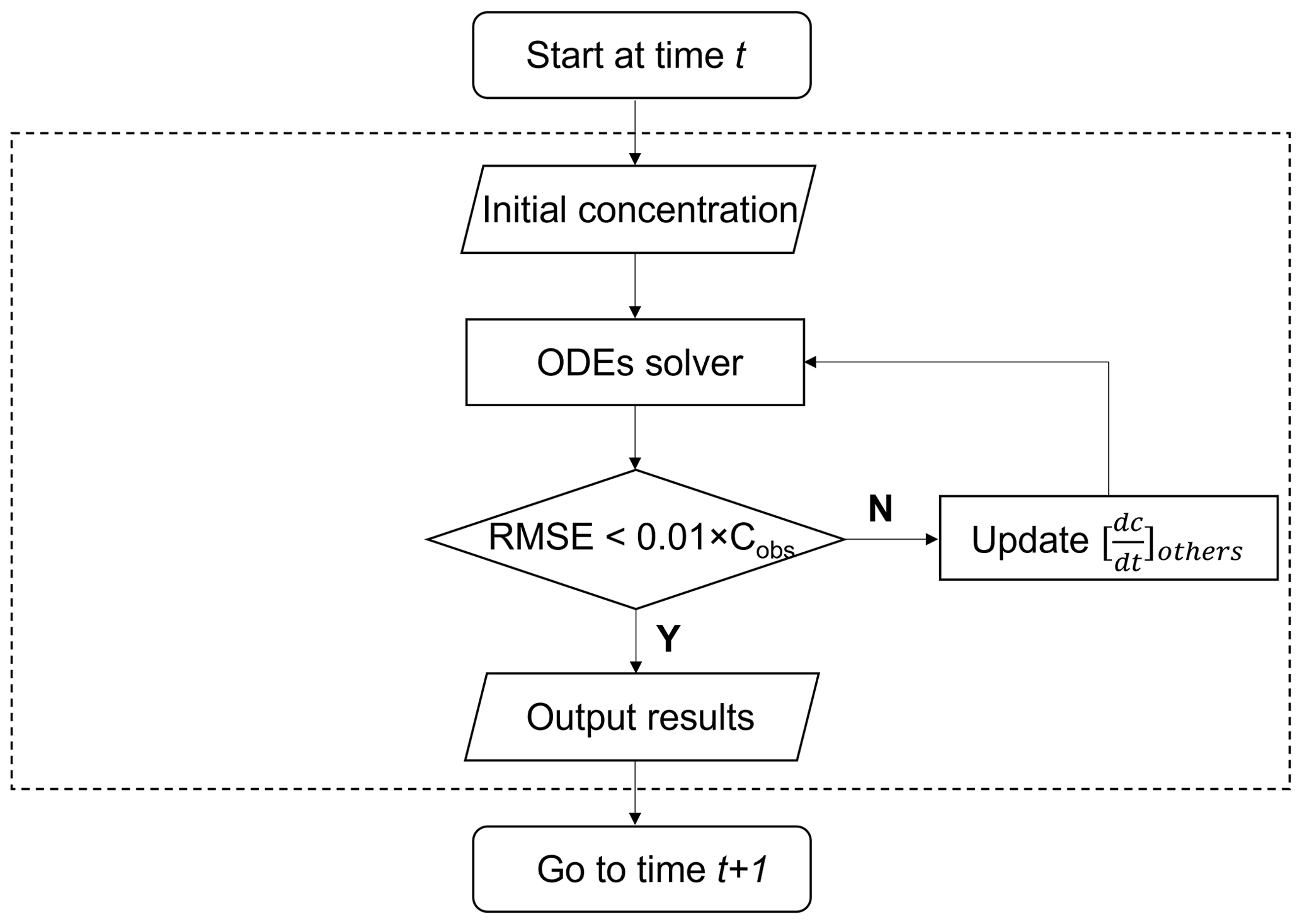
Scheme 1. Different from previous models, ROMAC provides a novel constraint scheme to use the observed data to constrain the model run. Scheme 1 does not directly input the species concentration, but controls the $[\frac{\mathrm{d}c}{\mathrm{d}t}{]}_{\mathrm{others}}$ term with adaptive dynamic optimization algorithm. The default value for $[\frac{\mathrm{d}c}{\mathrm{d}t}{]}_{\mathrm{others}}$ is 0, after integration, $\mathrm{\Delta }[\frac{\mathrm{d}c}{\mathrm{d}t}{]}_{\mathrm{others}}$ can be estimated by the gap between the observed and simulated values, as detailed in Eq. (28):

$$\begin{array}{}\text{(28)}& \mathrm{\Delta }{\left[{\displaystyle \frac{\mathrm{d}c}{\mathrm{d}t}}\right]}_{\mathrm{others}}=\left\{\begin{array}{l}\frac{C_{\mathrm{obs},n+\mathrm{1}}-C_{\mathrm{model},n+\mathrm{1}}}{t_{n+\mathrm{1}}-t_n}\\ \left(\mathrm{|}{C}_{\mathrm{obs},n+\mathrm{1}}-C_{\mathrm{model},n+\mathrm{1}}\mathrm{|}\le \mathrm{0.1}\right.\\ \left.\times \mathrm{|}{C}_{\mathrm{model},n+\mathrm{1}}\mathrm{|}\right)\\ \frac{\mathrm{0.1}\times C_{\mathrm{model},n+\mathrm{1}}}{t_{n+\mathrm{1}}-t_n}\times {\left(-\mathrm{1}\right)}^u\\ \left(\mathrm{|}{C}_{\mathrm{obs},n+\mathrm{1}}-C_{\mathrm{model},n+\mathrm{1}}\left|>\mathrm{0.1}\right.\right.\\ \left.\left.\times \mathrm{|}{C}_{\mathrm{model},n+\mathrm{1}}\right|\right)\end{array}\right.,\end{array}$$

where C_obs represents the observations and C_model represents the simulations. In Eq. (28), u=1 when $C_{\mathrm{obs},n+\mathrm{1}}$ is less than $C_{\mathrm{model},n+\mathrm{1}}$ and u=2 when $C_{\mathrm{obs},n+\mathrm{1}}$ is greater than $C_{\mathrm{model},n+\mathrm{1}}$. In complex systems, changing $[\frac{\mathrm{d}c}{\mathrm{d}t}{]}_{\mathrm{others}}$ may also affect other chemical process, and thus the relationship between $[\frac{\mathrm{d}c}{\mathrm{d}t}{]}_{\mathrm{others}}$ and the simulation results may be nonlinear. Therefore, it is difficult to calculate $[\frac{\mathrm{d}c}{\mathrm{d}t}{]}_{\mathrm{others}}$ in a single iteration. It is necessary to estimate this by loop iteration until the difference between observation and simulation reaches a preset tolerance. In this study, the difference between observation and simulation is characterized by the root mean square error (RMSE) shown in Eq. (29).

$$\begin{array}{}\text{(29)}& \text{RMSE}=\sqrt{(C_{\mathrm{obs},n+\mathrm{1}}-C_{\mathrm{model},n+\mathrm{1}}{)}^{\mathrm{2}}}\end{array}$$

The cyclic dynamic optimization process of ${\left[\frac{\mathrm{d}c}{\mathrm{d}t}\right]}_{\mathrm{others}}$ is shown in Fig. 1. The iterative updating formula of ${\left[\frac{\mathrm{d}c}{\mathrm{d}t}\right]}_{\mathrm{others}}$ based on the Newton–Raphson method is given in Eq. (30).

$$\begin{array}{}\text{(30)}& {\displaystyle }\begin{array}{rl}& {\left[{\displaystyle \frac{\mathrm{d}c}{\mathrm{d}t}}\right]}_{{\mathrm{others}}_{m+\mathrm{1}}}\\ & =\left\{\begin{array}{ll}{\left[\frac{\mathrm{d}c}{\mathrm{d}t}\right]}_{{\mathrm{others}}_m}+\mathrm{\Delta }{\left[\frac{\mathrm{d}c}{\mathrm{d}t}\right]}_{\mathrm{others}}& (m=\mathrm{1})\\ {\left[\frac{\mathrm{d}c}{\mathrm{d}t}\right]}_{{\mathrm{others}}_m}-{\text{RMSE}}_m\cdot {\left[\frac{\text{dRMSE}}{\mathrm{d}{\left[\frac{\mathrm{d}c}{\mathrm{d}t}\right]}_{\mathrm{others}}}\right]}_m^{-\mathrm{1}}& (m>\mathrm{1})\end{array}\right.\end{array}\text{(31)}& {\displaystyle }\begin{array}{rl}{\left[{\displaystyle \frac{\text{dRMSE}}{\mathrm{d}{\left[\frac{\mathrm{d}c}{\mathrm{d}t}\right]}_{\mathrm{others}}}}\right]}_m& ={\left[{\displaystyle \frac{\mathrm{\Delta }\text{RMSE}}{\mathrm{\Delta }{\left[\frac{\mathrm{d}c}{\mathrm{d}t}\right]}_{\mathrm{others}}}}\right]}_m\\ & ={\displaystyle \frac{{\text{RMSE}}_m-{\text{RMSE}}_{m-\mathrm{1}}}{{\left[\frac{\mathrm{d}c}{\mathrm{d}t}\right]}_{{\mathrm{others}}_m}-{\left[\frac{\mathrm{d}c}{\mathrm{d}t}\right]}_{{\mathrm{others}}_{m-\mathrm{1}}}}},\end{array}\end{array}$$

where m is the number of iterations and $\mathrm{\Delta }[\frac{\mathrm{d}c}{\mathrm{d}t}{]}_{\mathrm{others}}$ at the first iteration (m=1) is estimated by Eq. (28). When the number of iterations is greater than 1 (m>1), the update equation of $\mathrm{\Delta }[\frac{\mathrm{d}c}{\mathrm{d}t}{]}_{\mathrm{others}}$ is developed based on the Newton–Raphson method. The RMSE is used as the objective function for optimization, and the derivative of RMSE with $[\frac{\mathrm{d}c}{\mathrm{d}t}{]}_{\mathrm{others}}$ is estimated by the difference method shown in Eq. (31).

The $[\frac{\mathrm{d}c}{\mathrm{d}t}{]}_{\mathrm{others}}$ can also be optimized in the mode of kinetic equations (e.g., $[\frac{\mathrm{d}c}{\mathrm{d}t}{]}_{\mathrm{others}}=k_{\mathrm{others}}\times C$), and then the kinetic constants (k_others) can be optimized using a similar process shown in Fig. 1. ROMAC provides an option for the user to switch between these two modes. Furthermore, the user can also use other algorithms for dynamic optimization, such as ensemble Kalman filter (EnKF).

Figure 1 The cyclic dynamic optimization process of $[\frac{\mathrm{d}c}{\mathrm{d}t}{]}_{\mathrm{others}}$.

Scheme 2. In Scheme 2, the concentration of species can be initialized at the beginning of each simulation time step, which is mainly applied to the solution of initial value problems and more suitable for chamber simulation. This scheme has been widely used in previous models (e.g., PBM-MCM, AtChem, F0AM). However, if the regional transport process of pollutants is not considered, the simulation results of long-lived species in this scheme may have large deviations from the observed results.

Scheme 3. Scheme 3 constrains the change rate of species concentration ($\frac{\mathrm{d}c}{\mathrm{d}t}=\mathrm{0}$) while constraining the initial concentration, in a similar way as in F0AM. The advantage of this scheme is that the constrained variables can be kept at a user-specified level throughout the simulation. In this scheme, the long-lived species can maintain the observed concentration level. This constraining is appropriate if the temporal resolution of the observed data is high. The time interval of the model should be significantly smaller than the lifetime of constrained species. However, this approach also has its limitations. Since species concentrations are constrained as a constant, chemical imbalances may result.

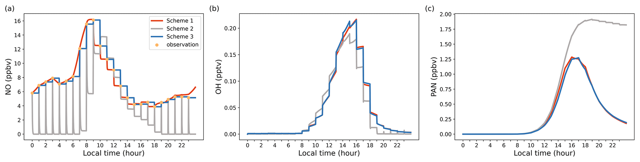
Figure 2 Model output results illustrating diurnal variations for selected species, highlighting the impact of different concentration constraint schemes. (a) NO concentrations; (b) OH concentrations; (c) PAN concentrations.

To better understand the distinctive attributes of various constraint schemes, we conducted a straightforward test case in which nitric oxide (NO) was constrained by three different schemes. Other input species (i.e., VOCs, NO₂, O₃, SO₂, CO) were constrained by Scheme 3. Figure 2 illustrates the results of this test, showcasing how different schemes affect the concentration of target species. The simulation utilized a time step of 120 s, while the input data interval from observations was set at 3600 s. Under Scheme 2, where emissions and regional transport were not considered, NO concentrations experienced a rapid decline before reaching a steady state (Fig. 2a). By contrast, both Scheme 1 and Scheme 3 displayed NO concentrations in close agreement with the observed hourly averages, ensuring that the model faithfully replicated the real atmospheric conditions. It is worth noting that due to variations in constraint schemes, simulated concentrations of other unconstrained species, such as OH and PAN, can also diverge (Fig. 2b and c). This case study was primarily designed to elucidate the unique features of different constraint schemes, with no intent to definitively validate or invalidate any particular scheme. Users are encouraged to make their scheme selections judiciously, aligning them with their specific research needs and observational findings.

2.3 Photolysis

ROMAC provides two ways for the user to set the photolysis rate. First, the user can specify the photolysis rate at each integration time step in the form of an ASCII file. The input photolysis rate can be estimated by other models or the observations. In ROMAC, a Python script (TUV2ROMAC.py) is provided for coupling the output of the Tropospheric Ultraviolet and Visible Radiation model (TUVv5.2, available at https://www2.acom.ucar.edu/modeling/tropospheric-ultraviolet-and-visible-tuv-radiation-model, last access: 6 May 2023). Users can easily use this tool to convert the TUV model output results into ROMAC input files.

ROMAC provides users with an inline calculation module to calculate photolysis. In the current version, the inline calculation module of photolysis uses the algorithm provided by MCM, an algorithm based on the solar zenith angle (SZA). The trigonometric parameterization function is shown in Eq. (32). The parameters of l, m, n are provided by MCM (http://mcm.york.ac.uk/, last access: 6 May 2023).

$$\begin{array}{}\text{(32)}& J=l\times \cos (\text{SZA}{)}^m\times e^{-n\times \text{sec(SZA)}}\end{array}$$

If both the input photolysis rate and the inline calculated photolysis rate are present, ROMAC will use the input photolysis rate preferentially. In addition, ROMAC provides the user with a photolysis rate modification factor (Jrate), which can easily be used to adjust the photolysis rate in the model. The default value of Jrate is 1.0, and the actual photolysis rate used in the model is the input rate or the inline calculated rate multiplied by Jrate.

2.4 Model accuracy and computational efficiency

The comparison of ROMAC with AtChem, F0AM and FACSIMILE, which is widely used for MCM, was performed on a PC with a CPU of 16-core AMD Ryzen 9 3950X at 3.5 GHz and 32 GB RAM. The operating system was 64 bit Ubuntu (version 20.04.1) and the software was compiled using Intel Fortran (ifort version 2021.2.0). The computational efficiency of the model is evaluated by CPU time. AtChem, ROMAC, and FACSIMILE are all run using a single core and the CPU time is recorded by the built-in function of the software. The CPU time used by F0AM is recorded by the function cputime in MATLAB. The total integration time is 345 600 s, and the integration time step is 900 s. The settings of atol (10⁻⁴) and rtol (10⁻³) in the models are consistent. The temperature, pressure and humidity in the scenario simulation are 25 ^∘C, 101.325 kPa and 35 %, respectively. The chemical mechanism used in this test is MCM v3.3.1, and the initial species concentrations are shown in Table A1. Since running the entire version of MCM v3.3.1 using AtChem is computationally excessive for our computing platform, we only selected the VOCs included in the EPA Photochemical Assessment Monitoring Stations (PAMS) Target List (https://www.epa.gov/amtic/, last access: 21 October 2023) and exported the mechanism file from the MCM website. In this test case, 3899 species and 11 814 chemical reactions were included.

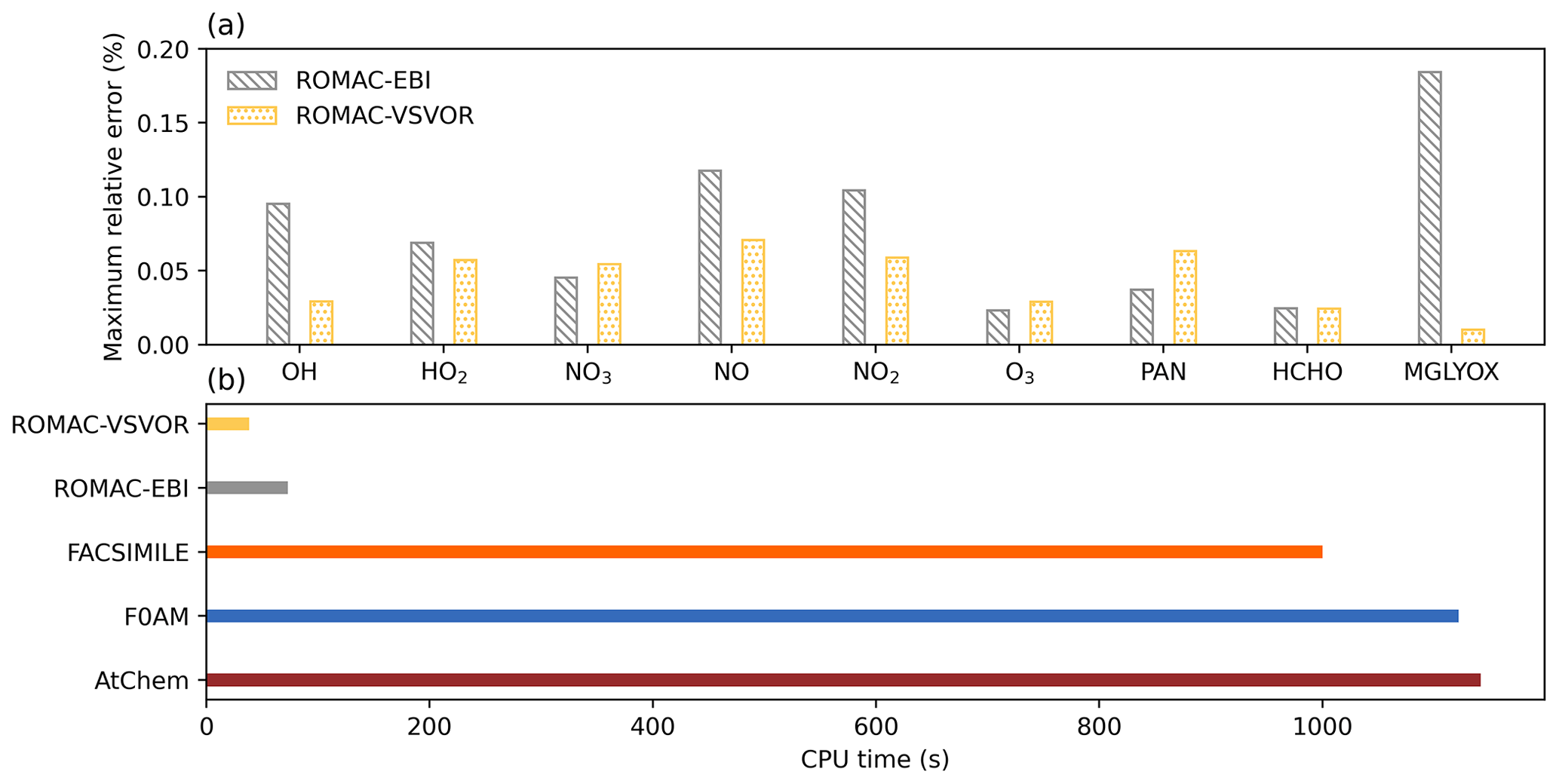
Figure 3 Accuracy evaluation and comparison of model computational efficiency. (a) Maximum relative error between the integration results of ROMAC and AtChem. (b) CPU time used to run compared with other models.

In this study, we assumed that the solution results of AtChem based on the CVODE library are accurate. Therefore, the accuracy of the model is evaluated by calculating the relative difference between the solution results of ROMAC and AtChem (Eq. 33).

$$\begin{array}{}\text{(33)}& {\text{RE}}_t={\displaystyle \frac{\mathrm{|}{C}_{\mathrm{ROMAC},t}-C_{\mathrm{AtChem},t}\mathrm{|}}{\mathrm{|}{C}_{\mathrm{AtChem},t}\mathrm{|}}}\times \mathrm{100}\mathit{\%}\end{array}$$

Figure A1 shows a comparison of simulation results for nine species, including radicals and gaseous pollutants, which were commonly used in previous studies to evaluate solution results (Hertel et al., 1993; Esentürk et al., 2018; Aro, 1996b). The simulation results for ROMAC in Fig. A1 are processed by the VSVOR solver. As shown in Fig. A1, the solution results of ROMAC and AtChem are comparable, indicating that the solution results of ROMAC are comparable to the high-precision solution algorithm. The time series of relative error and its growth rates are depicted in Fig. A2. The relative difference between the solution results of ROMAC and that of AtChem is gradually stabilized, and the rate of change of the relative error after 270 000 s is extremely low, between $-\mathrm{1.0}\times {\mathrm{10}}^{-\mathrm{6}}$ % s⁻¹ and $\mathrm{1.0}\times {\mathrm{10}}^{-\mathrm{6}}$ % s⁻¹. Although the relative error of O₃ has a trend of continuous increase, the growth rate of the error remains stable and extremely low ($\mathrm{3.3}\times {\mathrm{10}}^{-\mathrm{8}}$ % s⁻¹). Hence, the relative error remains within the preset rtol even if the simulation duration is extended by an additional 2.0×10⁶ s at this growth rate. This suggests that the error of the ROMAC result can be stably controlled during long-term simulations. Figure 3 illustrates the maximum relative error in the scenario simulation and the CPU time used by each model. The maximum relative errors between the results of the VSVOR solver and the results of AtChem are all smaller than the preset rtol. The solution results obtained from the EBI solver were also evaluated in this study. The discrepancy of certain species in the results obtained by EBI exceeds the preset tolerance (0.1 %), such as NO, NO₂ and MGLYOX. Compared with the single-step EBI solver, the VSVOR solver with variable time step and variable order can better control the truncation error. In terms of CPU time required for execution, the VSVOR solver with higher solution accuracy is even more efficient than EBI. The CPU time consumed by EBI with different integration time steps is shown in Table A2. For the MCM chemical mechanism, the algorithm fails to converge when the integration time step is longer than 50 s. After a series of tests, we found that even with an integration time step of 10 s, the EBI solver was at risk of failing to converge. However, reducing the integration time step too much diminishes the efficiency of the EBI solver when handling the MCM mechanism in comparison to the VSVOR solver. Hence, the VSVOR solver exhibits comparable computational efficiency to the EBI solver, while maintaining superior solution accuracy and stability.

Compared with other models, ROMAC has greatly improved the computational efficiency of solving large-scale chemical mechanisms. The computational efficiency of ROMAC is 97 % higher than that of F0AM and AtChem, and 96 % higher than that of FACSIMILE.

3 Model validation and application

3.1 Chamber simulation case

A chamber experiment for toluene degradation was used to evaluate the capabilities of ROMAC to dynamically optimize chemical and physical processes. In this case, the indoor smog chamber in JNU-VMDSC was used to simulate the degradation of toluene. The JNU-VMDSC provides a reliable experimental platform, and its structure and characterization ($e.g.,$ wall loss, light intensity, airtightness test) have been described in a previous study (W. Wang et al., 2023). Toluene and isoprene were injected into the chamber before the UV light was turned on. The initial mixing ratios of toluene and isoprene were 2157 and 160 ppbv, respectively.

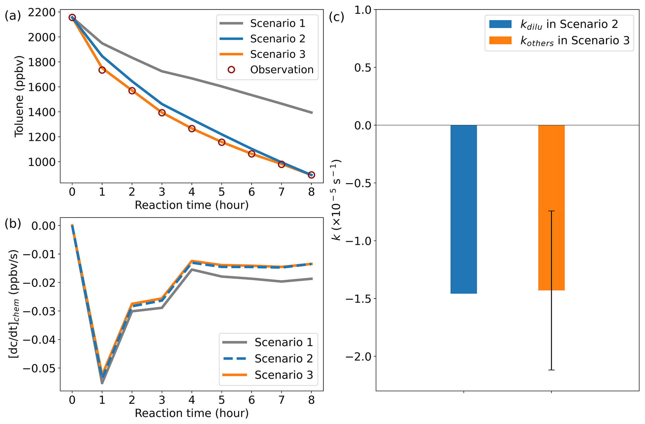
Figure 4 Model simulation results. (a) Comparison results between the simulated and observed toluene mixing ratios. (b) Chemical loss rate of toluene. (c) Comparison of kinetic constants in dilution process. Error bars indicate the standard deviation of k_others at different times in scenario 3.

In order to simulate the effect of the dilution process on the toluene concentration, nitrogen was injected into the chamber at a flow of 7 L min⁻¹, while sampling was carried out at a flow of 7 L min⁻¹ at the sampling port. Similar to previous studies (Dada et al., 2020; Jiang et al., 2020), the rate of dilution was calculated using Eqs. (34) and (35):

$$\begin{array}{}\text{(34)}& {\displaystyle }{\left[{\displaystyle \frac{\mathrm{d}c}{\mathrm{d}t}}\right]}_{\mathrm{dilu}}={\displaystyle \frac{C\times \mathrm{d}v}{V_{\mathrm{chamber}}\times \mathrm{d}t}}=k_{\mathrm{dilu}}\times C\text{(35)}& {\displaystyle }{k}_{\mathrm{dilu}}={\displaystyle \frac{\mathrm{1}}{V_{\mathrm{chamber}}}}\times {\displaystyle \frac{\mathrm{d}v}{\mathrm{d}t}}={\displaystyle \frac{\text{Flow}}{V_{\mathrm{chamber},}}}\end{array}$$

where k_dilu is the rate constant of dilution, V_chamber is the volume of the chamber (8000 L), and “Flow” is the flow of nitrogen injection. Therefore, the theoretical estimation result of k_dilu in this case is $\mathrm{1.458}\times {\mathrm{10}}^{-\mathrm{5}}$ s⁻¹. Wall loss was not considered in this simple experiment with gaseous pollutants.

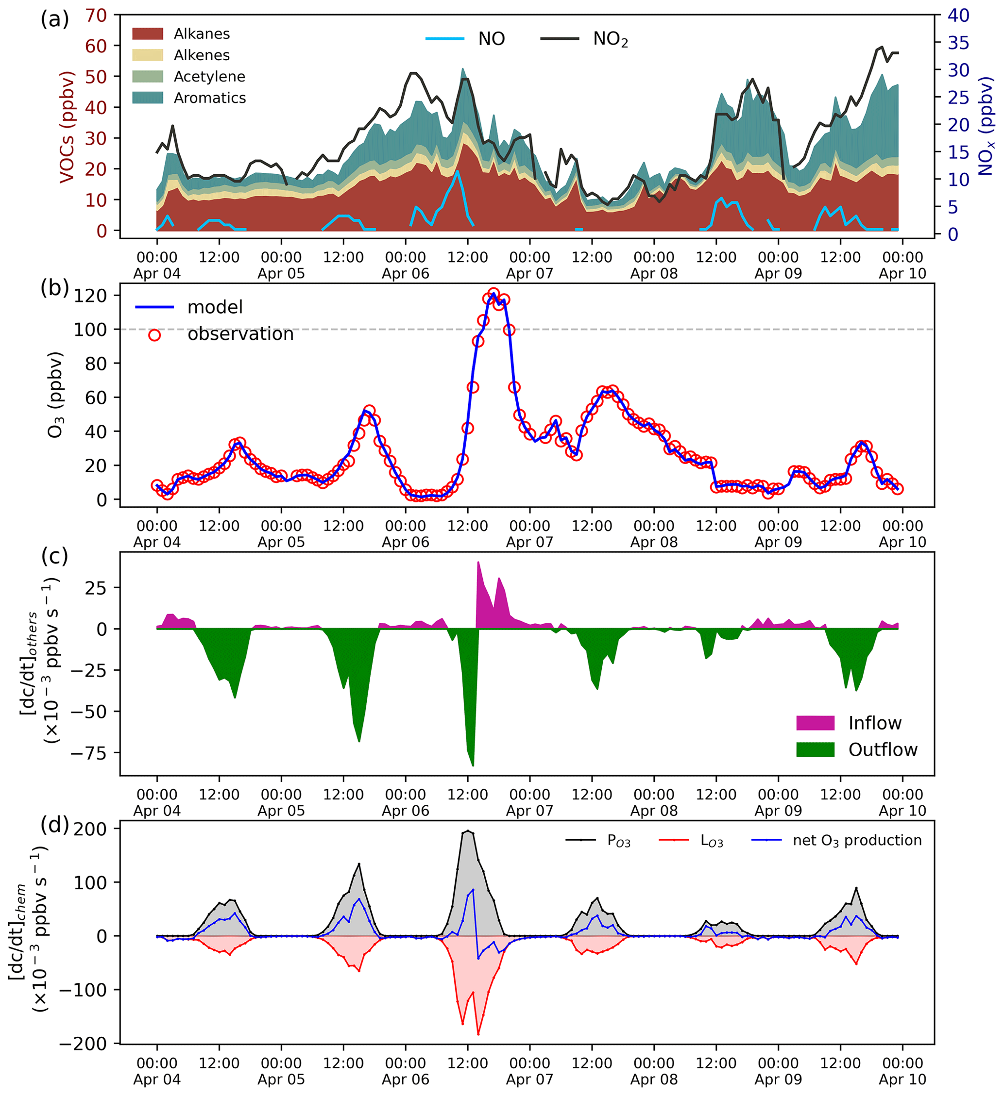
Figure 5 Species mixing ratio and the rate of O₃ change. (a) VOCs and NO_x mixing ratios. (b) Model and observation O₃ mixing ratios. (c) The effect of the physical process on the O₃ mixing ratios calculated by the adaptive dynamic optimization module. (d) The rate of O₃ chemical production.

The version of the chemical mechanism used in the model simulations is MCM v3.3.1, all species and mechanisms in MCM are included. Three case scenarios were set up to evaluate the simulation capabilities of ROMAC. In scenario 1, only chemical processes were considered (Eq. 36). In scenario 2, chemical processes and dilution processes were considered (Eq. 37). In scenario 3, we assume that the results of the experiment are influenced by an unknown process, and this process is assumed to be a first-order kinetic process (Eq. 38). The k_others in scenario 3 was dynamically optimized with Scheme 1 as described in Sect. 2.2. Theoretically, the value of k_others obtained by the dynamic optimization in scenario 3 should be close to k_dilu in scenario 2.

$$\begin{array}{}\text{(36)}& {\displaystyle \frac{\mathrm{d}{c}_{\mathrm{Tolu}}}{\mathrm{d}t}}={\left[{\displaystyle \frac{\mathrm{d}{c}_{\mathrm{Tolu}}}{\mathrm{d}t}}\right]}_{\mathrm{chem}}\text{(37)}& {\displaystyle }\begin{array}{rl}{\displaystyle \frac{\mathrm{d}{c}_{\mathrm{Tolu}}}{\mathrm{d}t}}& ={\left[{\displaystyle \frac{\mathrm{d}{c}_{\mathrm{Tolu}}}{\mathrm{d}t}}\right]}_{\mathrm{chem}}+{\left[{\displaystyle \frac{\mathrm{d}{c}_{\mathrm{Tolu}}}{\mathrm{d}t}}\right]}_{\mathrm{dilu}}\\ & ={\left[{\displaystyle \frac{\mathrm{d}{c}_{\mathrm{Tolu}}}{\mathrm{d}t}}\right]}_{\mathrm{chem}}+k_{\mathrm{dilu}}\times C_{\mathrm{Tolu}}\end{array}\text{(38)}& {\displaystyle }\begin{array}{rl}{\displaystyle \frac{\mathrm{d}{c}_{\mathrm{Tolu}}}{\mathrm{d}t}}& ={\left[{\displaystyle \frac{\mathrm{d}{c}_{\mathrm{Tolu}}}{\mathrm{d}t}}\right]}_{\mathrm{chem}}+{\left[{\displaystyle \frac{\mathrm{d}{c}_{\mathrm{Tolu}}}{\mathrm{d}t}}\right]}_{\mathrm{others}}\\ & ={\left[{\displaystyle \frac{\mathrm{d}{c}_{\mathrm{Tolu}}}{\mathrm{d}t}}\right]}_{\mathrm{chem}}+k_{\mathrm{others}}\times C_{\mathrm{Tolu}}\end{array}\end{array}$$

The total duration of the chamber experiment was 8 h, and the CPU time consumed by a single simulation of ROMAC was about 13 s. Figure 4 illustrates the comparison results between the simulated and observed toluene mixing ratios for different scenario cases. Due to the lack of dilution process in scenario 1, there is a large gap between simulation results and observations. After considering the dilution process, the simulation of scenario 2 was improved, which indicates that the setting of scenario 2 is reasonable. The absence of a physical process in the model is identified as the primary cause for failure to reproduce observations in scenario 1. The simulation results of scenario 3 agree well with the observations, which indicates that the dynamic optimization algorithm successfully captures the process that cannot be explained by the MCM chemical mechanism. Figure 4b illustrates the chemical loss rate of toluene under different simulation scenarios. The results of scenario 3 and scenario 2 are consistent and significantly different from the results of scenario 1. This indicates that the dynamic optimization algorithm can improve the chemical process while optimizing the physical process. Ignoring physical processes in the traditional box model may introduce large uncertainty to the simulation results. The rate of the physical process is subject to uncertainty in practical applications, but its average value is expected to closely approximate the theoretical value. The optimized value of k_others in scenario 3, as shown in Fig. 4c, exhibits a certain range of fluctuations rather than a fixed value. However, its average values ($\mathrm{1.430}\times {\mathrm{10}}^{-\mathrm{5}}$) are comparable to k_dilu in scenario 2 (Fig. 4c), which indicates that the dynamically optimized algorithm is reliable.

3.2 Field observation case

This case demonstrates the application of ROMAC to the analysis of the photochemical process of O₃ formation and the dynamic optimization of physical processes. The observation data were obtained at the Heshan Atmospheric Supersite (22.728^∘ N, 112.929^∘ E) in Guangdong Province, China. A detailed description of the Heshan site can be found in previous publications (He et al., 2019; Yang et al., 2017). The observation period was from 4 to 10 April 2021. Meteorological parameters and the mixing ratios of NO_x, VOCs, SO₂, CO were constrained by Scheme 3. The concentrations of NO_x and VOCs were shown in Fig. 5a, with the meteorological observations in Fig. A3.

Figure 6 RIR values of O₃ precursors, i.e., VOCs, NO_x and CO.

The simulation of O₃ was constrained by Scheme 1. In this case, all physical processes of O₃ (e.g., dry deposition, dilution, transport) were merged into $[\frac{\mathrm{d}{c}_{{\mathrm{O}}_{\mathrm{3}}}}{\mathrm{d}t}{]}_{\mathrm{others}}$. The rate of change of O₃ is shown in Eq. (39). The optimal estimate of $[\frac{\mathrm{d}{c}_{{\mathrm{O}}_{\mathrm{3}}}}{\mathrm{d}t}{]}_{\mathrm{others}}$ uses Scheme 1 shown in Fig. 1.

$$\begin{array}{}\text{(39)}& {\displaystyle \frac{\mathrm{d}{c}_{{\mathrm{O}}_{\mathrm{3}}}}{\mathrm{d}t}}={\left[{\displaystyle \frac{\mathrm{d}{c}_{{\mathrm{O}}_{\mathrm{3}}}}{\mathrm{d}t}}\right]}_{\mathrm{chem}}+{\left[{\displaystyle \frac{\mathrm{d}{c}_{{\mathrm{O}}_{\mathrm{3}}}}{\mathrm{d}t}}\right]}_{\mathrm{others}}\end{array}$$

The comparison between the optimized simulation results and the observations of O₃ mixing ratios is shown in Fig. 5b. As expected, the model outputs are consistent with the observations due to the dynamic optimization. The estimated value of ${\left[\frac{\mathrm{d}{c}_{{\mathrm{O}}_{\mathrm{3}}}}{\mathrm{d}t}\right]}_{\mathrm{others}}$ for the physical process is shown in Fig. 5c. Positive values of ${\left[\frac{\mathrm{d}{c}_{{\mathrm{O}}_{\mathrm{3}}}}{\mathrm{d}t}\right]}_{\mathrm{others}}$ indicate that physical processes increase local O₃ concentration (e.g., external transport), while negative values indicate a decrease in O₃ concentration (e.g., dilution, deposition). As displayed in Fig. 5c, ${\left[\frac{\mathrm{d}{c}_{{\mathrm{O}}_{\mathrm{3}}}}{\mathrm{d}t}\right]}_{\mathrm{others}}$ is usually negative during the daytime, indicating that O₃ was transported out of the region after formation by photochemical processes. However, positive values of ${\left[\frac{\mathrm{d}{c}_{{\mathrm{O}}_{\mathrm{3}}}}{\mathrm{d}t}\right]}_{\mathrm{others}}$ can also occur during the daytime. On 6 April, the surface ozone mixing ratio increased rapidly, and the maximum hourly mixing ratio exceeded China II Emission Standard (>100 ppbv). The value of ${\left[\frac{\mathrm{d}{c}_{{\mathrm{O}}_{\mathrm{3}}}}{\mathrm{d}t}\right]}_{\mathrm{others}}$ on the afternoon of 6 April is positive, indicating that physical processes were one of the reasons for the occurrence of O₃ pollution.

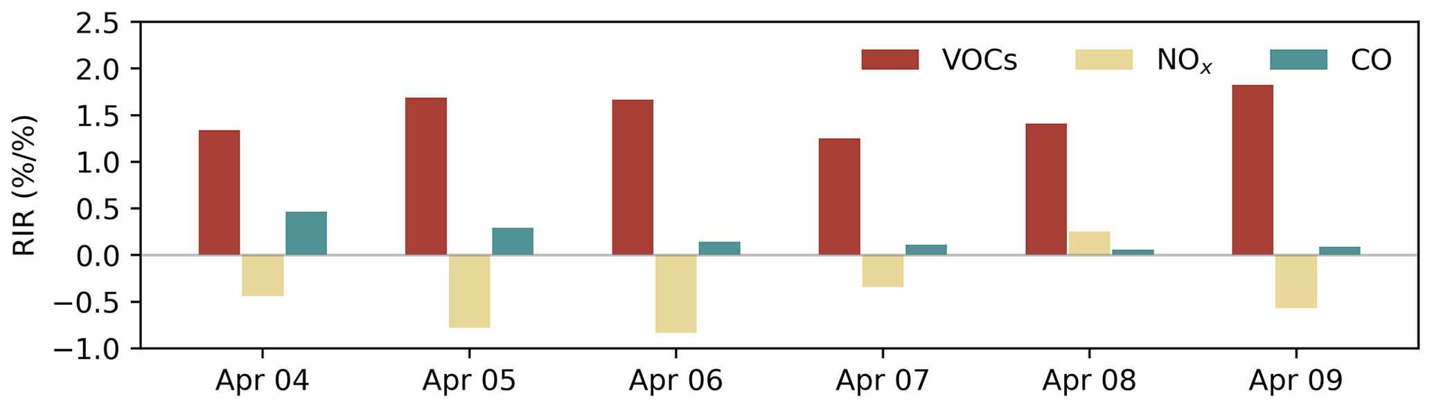
The rate of O₃ chemical production and precursor sensitivities were calculated using a method described in previous studies (Liu et al., 2022; Wang et al., 2018). As displayed in Fig. 5d, the net O₃ production rate on 6 April 2021 was significantly higher than that on other days, indicating that chemical processes were also an important cause of O₃ pollution. The sensitivity of the O₃ formation to its precursors can be represented by relative incremental reactivity (RIR). Figure 6 shows the daily average RIR values of VOCs, NO_x and CO. The RIR values of VOCs and CO were positive, which indicates that reducing the concentration of VOCs and CO can effectively reduce the chemical formation of O₃. Except for 8 April, the RIR values of NO_x were negative, indicating that decreasing the NO_x concentration leads to an increase in O₃ concentration. The negative values of RIR for NO_x and higher positive values of RIR for VOC indicate that the ozone formation at the Heshan Atmospheric Supersite was mostly likely under a VOC limited regime. The result was consistent with a previous study (He et al., 2019), indicating that the application of ROMAC in chemical process diagnosis is reliable.

The application of this case demonstrates the ability of ROMAC to quantify the contribution of physical and chemical processes to air pollutant concentrations. Compared with the traditional observation-based box model (OBM), ROMAC is superior in evaluating the impact of physical processes on pollutant concentrations. Compared with emission-based 3-D air quality models (e.g., CMAQ, WRF-Chem, NAQPMS), the observation-based dynamic optimization algorithm in ROMAC reduces the uncertainty introduced by emission inventory and meteorological simulation.

4 Future developments

ROMAC will be continuously updated and developed. Functionality for future improvements and upgrades includes the following:

• A multiphase chemical reaction module and a module for gas–particle partitioning and sectional simulation are being developed.

• Adjoint sensitivity analysis will be added in a future version, and users can use ROMAC to analyze the relationship between precursors and secondary pollutants.

• The ensemble Kalman filter (EnKF) will be added to dynamically optimize the physical process in future versions.

• In a future development roadmap, we have plans to introduce a modeling framework version of ROMAC known as “ROMAC plug-in.” This ROMAC plug-in will support calls from Python or Fortran, ensuring compatibility and flexibility for users. Importantly, the efficient design of ROMAC will be maintained, allowing for an optimized performance. The kernel of the ROMAC plug-in will be specifically engineered to provide users with flexibility to effortlessly construct their own models or integrate ROMAC with existing frameworks, such as CTMs.

Appendix A

Table A1 Initial species concentration used for model comparisons (unit: molecules cm⁻³).

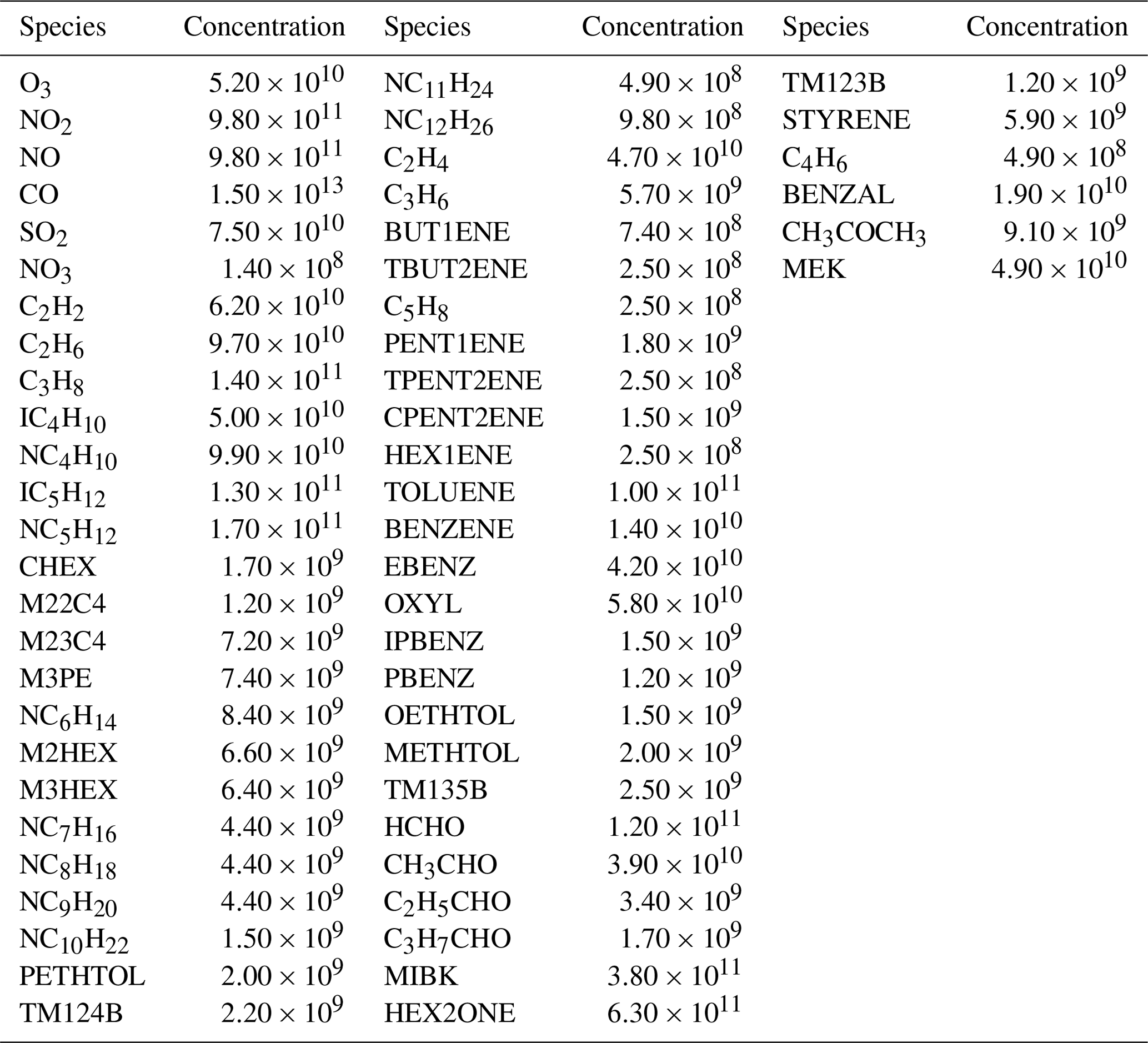
Table A2 CPU time used by the EBI solver at different integration time step sizes (unit: seconds). “Nonconvergence” represents that the EBI solver fails to converge.

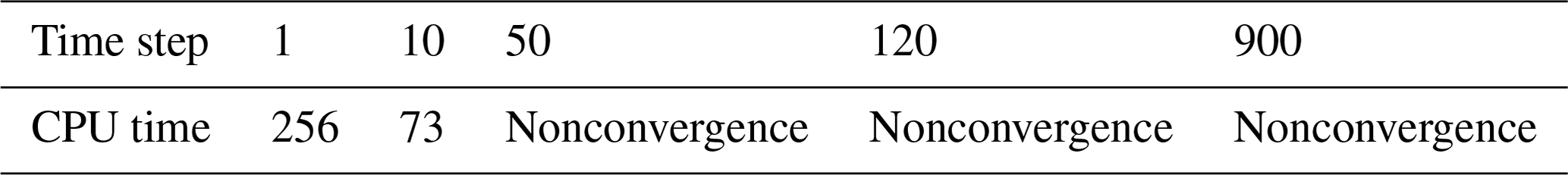
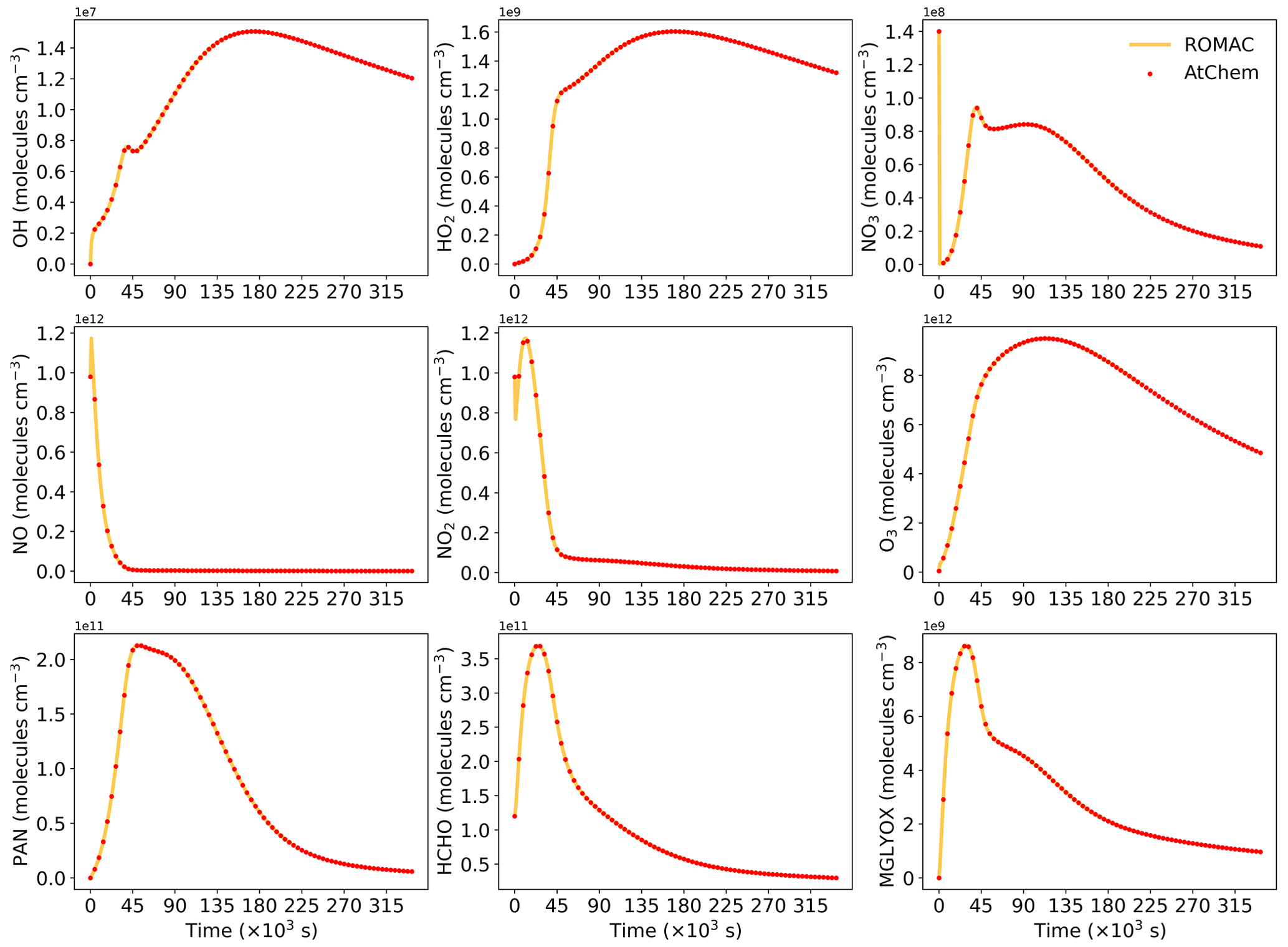
Figure A1 Comparison of the simulation results between ROMAC and AtChem for nine substances. ROMAC used the VSVOR solver in this test.

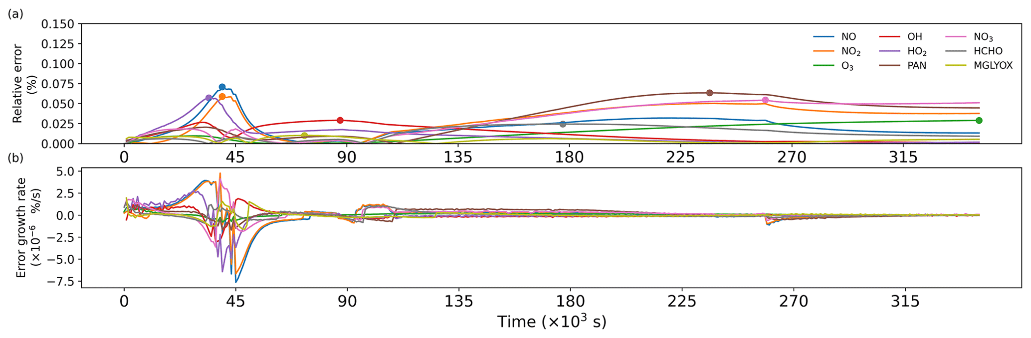
Figure A2 (a) Time series of relative errors, with dots marking the maximum values. (b) Growth rate of relative errors.

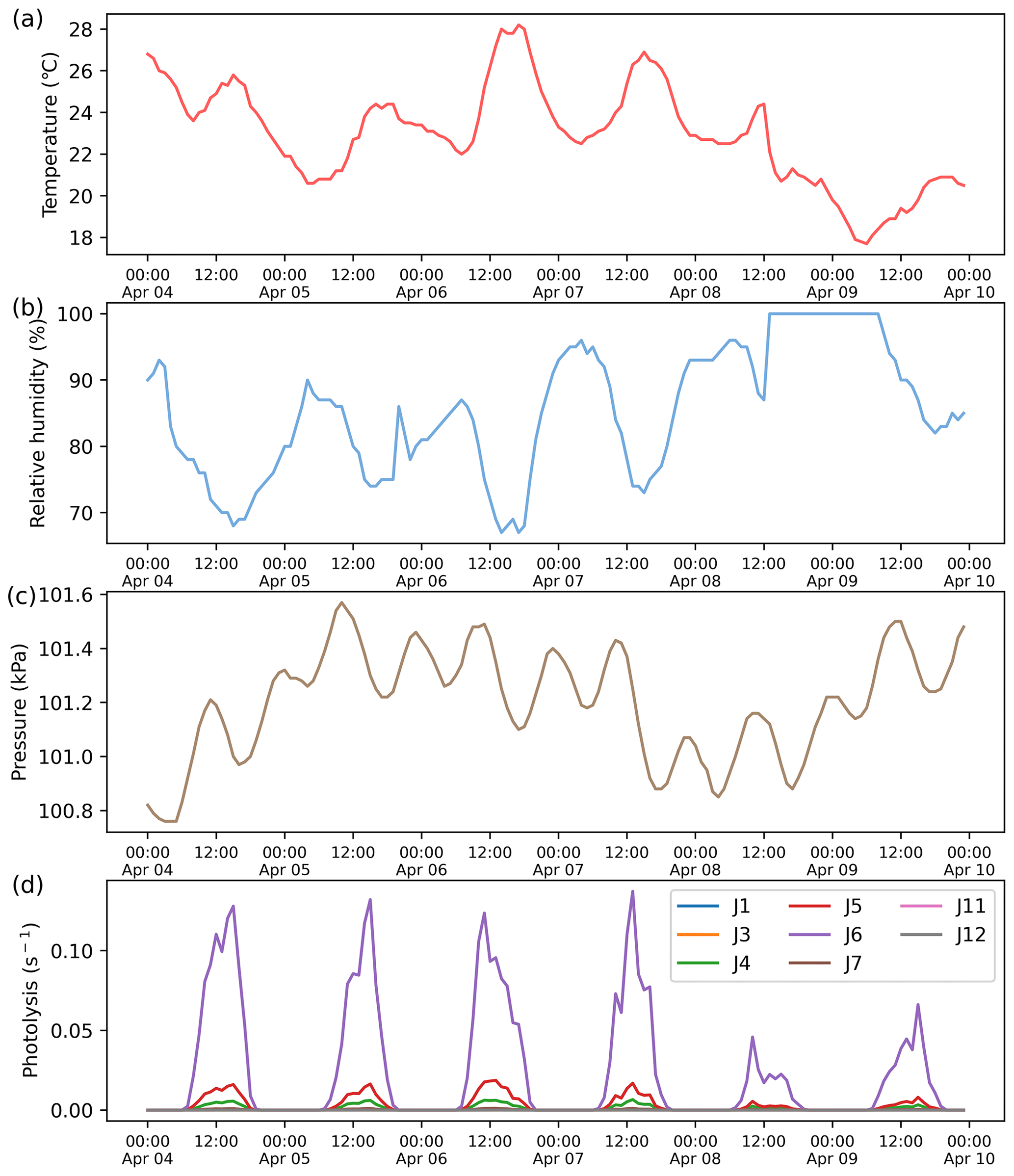
Figure A3 Meteorological data input to the model. (a) Temperature. (b) Relative humidity. (c) Atmospheric pressure. (d) Photolysis rate.

Appendix B: Nomenclature

ODEs	Ordinary differential equations
VSVOR	Variable-step and variable-order solver
atol	absolute tolerance
rtol	relative tolerance
r	The reactant in a chemical reaction
p	The product in a chemical reaction
α, β	Stoichiometric number
Ct	Concentration of species at time t
$f_i\left(C_{i,t},t\right)$	Rate of change of species i at time t
Pi,t	Product rate of species i at time t
Li,t	Loss rate of species i at time t
$l_{i,t,R}$	The part of the chemical reaction rate that is not directly related to the concentration of species i in reaction R at time t
Δt	Integration time step size
g1(Ct+1)	The objective function when Newton's method solves the implicit Euler method
g2(Ct+1)	The objective function when Newton's method solves the implicit trapezoidal method
$C_{t+\mathrm{1}}^k$	Species concentration at iteration k of Newton's method
∇g1(Ct+1)	The Jacobian matrix of g1(Ct+1)
∇g2(Ct+1)	The Jacobian matrix of g2(Ct+1)
$\mathrm{\nabla }{g}^{-\mathrm{1}}\left(C_{t+\mathrm{1}}\right)$	The inverse of the Jacobian matrix
Δt0	Integration time step size equal to $\mathrm{2.22}\times {\mathrm{10}}^{-\mathrm{16}}$ s
Δt1	Minimum species atmospheric lifetime in chemical mechanisms
Δt2	The maximum time step size necessary to achieve diagonal dominance of the Jacobian matrix.
Δtinit	Initial integration time step size
Δtmax	The maximum integration time step to ensure the result does not exceed the preset tolerance
Δtopt	Optimal integration step size
RERR	Relative error calculated by doubled-step method
LTE	Local truncation error
atol	Absolute tolerance
rtol	Relative tolerance
Rn	Lagrangian remainder in the Taylor expansion
ξ	Real number in the Lagrangian remainder in the Taylor expansion
RMSE	Root mean square error