the Creative Commons Attribution 4.0 License.
the Creative Commons Attribution 4.0 License.
 | 26 Jan 2023
Evaluation of a cloudy cold-air pool in the Columbia River basin in different versions of the High-Resolution Rapid Refresh (HRRR) model
James M. Wilczak
Jaymes Kenyon
Laura Bianco
Irina V. Djalalova
Joseph B. Olson
David D. Turner
The accurate forecast of persistent orographic cold-air pools in numerical weather prediction models is essential for the optimal integration of wind energy into the electrical grid during these events. Model development efforts during the second Wind Forecast Improvement Project (WFIP2) aimed to address the challenges related to this. We evaluated three versions of the National Oceanic and Atmospheric Administration (NOAA) High-Resolution Rapid Refresh model with two different horizontal grid spacings against in situ and remote sensing observations to investigate how developments in physical parameterizations and numerical methods targeted during WFIP2 impacted the simulation of a persistent cold-air pool in the Columbia River basin. Differences amongst model versions were most apparent in simulated temperature and low-level cloud fields during the persistent phase of the cold-air pool. The model developments led to an enhanced low-level cloud cover, resulting in better agreement with the observations. This removed a diurnal cycle in the near-surface temperature bias at stations throughout the basin by reducing a cold bias during the night and a warm bias during the day. However, low-level clouds did not clear sufficiently during daytime in the newest model version, which leaves room for further model developments. The model developments also led to a better representation of the decay of the cold-air pool by slowing down its erosion.
- Article
(8232 KB) - Full-text XML
- BibTeX
- EndNote


Persistent cold-air pools (hereafter cold pools) frequently form during wintertime in orographic basins and valleys; during this period, the air near the surface cools and/or the air aloft warms, leading to an increase in temperature with height (e.g., Whiteman et al., 2001). Wind speed within the cold pools is generally weak and rapidly accelerates during its decay. As many wind turbines have a cut-in speed of around 3 m s−1, the wind energy produced during cold-pool events is typically small (e.g., Bianco et al., 2016; Wilczak et al., 2019). At the end of the events, wind energy production often jumps to very large values, so-called wind energy ramps, because wind power increases approximately as the cube of the wind speed. Forecast errors in wind speed and cold-pool decay time were found to be reduced by an improved representation of the cold pool's vertical structure and depth (e.g., Olson et al., 2019b). To more efficiently integrate the wind energy produced during cold-pool events into the electrical grid, accurate forecasts of the evolution and structure of these events are necessary (e.g., Wilczak et al., 2019; Olson et al., 2019b). Cold pools are complex, and their evolution and structure depends on a variety of atmospheric processes including large-scale advection and subsidence; mesoscale flows; and radiative, turbulent, and cloud processes (e.g., Lareau et al., 2013). This makes it challenging for numerical weather prediction models to correctly represent the cold-pool structure and evolution (e.g., Reeves et al., 2011; Holtslag et al., 2013; Olson et al., 2019b). Numerical simulations indicate that the relative importance of the different processes varies from one cold pool to another and may depend on the geographic location, terrain characteristics, season of the year, large-scale conditions, and snow cover (e.g., Zhong et al., 2001; Wei et al., 2013; Lu and Zhong, 2014; Neemann et al., 2015; Lareau and Horel, 2015; Crosman and Horel, 2017).
Low-level clouds can have a strong impact on the temporal evolution and vertical structure of temperature in cold pools. While cloud-free cold pools usually have a surface-based temperature inversion in which stability decreases smoothly with height, cloudy cold pools often have a near-moist adiabatic lapse rate in the sub-cloud and cloud layer which is topped by a strong elevated temperature inversion (Whiteman et al., 2001). Strong longwave radiative cooling at cloud top causes the elevated temperature inversion and can induce top-down turbulent mixing (e.g., Adler et al., 2021). Increased mixing near the surface in cloudy cold pools was found to be associated with lower pollutant concentrations compared with cloud-free conditions (e.g., VanReken et al., 2017). The composition of the low-level clouds, whether ice-dominant or liquid-dominant clouds, was found to be relevant for the vertical structure of simulated wintertime cold pools (Neemann et al., 2015). When ice-phase particles dominated, the cloudy layer was shallower and temperature near the surface was lower compared with liquid-dominant clouds. These authors found that ice-dominant clouds gave the best agreement between observed and simulated temperature profiles and cloud occurrences. In the presence of clouds, the diurnal temperature cycle near the surface is weakened due to reduced shortwave downward radiation flux during daytime and reduced longwave net radiation flux during nighttime (e.g., Sun and Holmes, 2019). Too few simulated nocturnal low-level clouds can lead to large cold biases in the simulated near-surface temperature during nights when low-level clouds are observed, as they reduce longwave outgoing radiation flux (e.g., Hughes et al., 2015) and increase downward longwave radiation flux below the clouds. On the other hand, daytime low-level clouds can help to maintain the cold pool, as they reduce convective heating (e.g., Zhong et al., 2001). This is especially relevant during spring and fall when insolation is strong. The failure of models to produce realistic low-level clouds can thus lead to an erroneous erosion of the cold pool during daytime under certain conditions.
To improve the forecast for wind energy applications in complex terrain, the second Wind Forecast Improvement Project (WFIP2) was initiated by the Department of Energy in 2015 (Shaw et al., 2019). The target area was the Columbia River basin in Washington and Oregon in the Pacific Northwest of the United States, which is home to a large amount of wind energy production (more than 6 GW at the time of the project) and is often affected by cold pools (McCaffrey et al., 2019), gap flows (Neiman et al., 2019), and mountain waves (Draxl et al., 2021) – atmospheric phenomena which are all relevant for wind energy forecasts (Wilczak et al., 2019). Besides completing a comprehensive 18-month-long field campaign (Wilczak et al., 2019) and developing support tools to assist the industry in wind power forecasting, model development efforts were a key component of WFIP2 (Olson et al., 2019b). The basis for the model developments were the National Oceanic and Atmospheric Administration (NOAA) Rapid Refresh (RAP; Benjamin et al., 2016) and High-Resolution Rapid Refresh (HRRR; Dowell et al., 2022) models. In this study, we used three versions of the HRRR model to evaluate how the model developments impacted the characteristics of a strong and persistent cold-pool event in the Columbia River basin, which occurred within a 10 d period from 10 to 19 January 2017. Note that we did not investigate the sensitivity to the individual changes in physical parameterization and numerical methods but rather evaluated the model developments as a whole.
The observed evolution and structure of this cold-pool event, as well as the involved processes, were investigated in detail by Adler et al. (2021) using the comprehensive observational data set gathered during the WFIP2 field campaign and surface measurements from several hundred surface stations available from the MesoWest repository (Horel et al., 2002). Adler et al. (2021) found that the cold-pool structure was strongly modulated by the presence of low-level clouds and that its temporal evolution was largely driven by synoptic-scale processes, i.e., horizontal advection and subsidence. The cold pool decayed when a low-pressure system approached the area and warm air gradually descended into the basin decreasing the cold-pool depth, accompanied by strong downslope winds on the southern slopes of the basin. The same cold-pool event was chosen for two numerical studies to address the impact of modified physical parameterizations. Arthur et al. (2022) investigated the effects of different planetary boundary layer (PBL) schemes and horizontal diffusion treatment on the representation of the cold pool. These authors found that computing horizontal diffusion in physical space and using a 3D PBL scheme better represented the vertical wind and temperature structure in the cold pool and its decay compared with a standard 1D PBL scheme. Berg et al. (2021) examined the sensitivity of wind speed at turbine hub height to parameters in the Mellor–Yamada–Nakanishi–Niino eddy-diffusivity mass-flux scheme (MYNN-EDMF) parameterization using the same cold-pool event as an example for a winter period. They found a high bias in hub height wind speed which was fairly insensitive to changes in the parameter values and concluded that the representation of cold-pool dynamics cannot be improved with changes in the MYNN-EDMF parameterization. In addition, as the mass-flux component of the EDMF parameterization was rarely triggered during the cold-pool event, there was little sensitivity to these parameters.
In this study, we first evaluate how the model developments targeted during WFIP2 impact the cold-pool characteristics during its maintenance and decay phase by comparing 24 h reforecasts for the three model versions to observations (Sect. 3). This includes the comparison of simulated and observed temperature and wind speed profiles (Sect. 3.2) as well as the cold-pool strength (Sect. 3.3) computed from ground-based remote sensing instruments. Using a large number of surface stations distributed in the basin, we further investigated the dependence of the near-surface temperature bias on station height and related differences between the model versions to differences in low-level cloud cover using downward shortwave and longwave radiation fluxes as proxies (Sect. 3.4). In a second step, we investigate how well the newest model version performed when extending the reforecast horizon to 48 h by comparing the first 24 h of the reforecasts to the last 24 h (Sect. 4). We started by assessing differences in temperature and cloud profiles (Sect. 4.1), followed by an investigation on how differences in the cold-pool thermodynamic structure during its maintenance phase may impact its decay (Sect. 4.2). In a final step, we evaluated differences in the near-surface temperature bias and its relationship to clouds (Sect. 4.3).
The Columbia River basin is a large basin in Washington and Oregon that is several hundred kilometers in diameter and is bordered by the north–south oriented Cascade Range to the west (Fig. 1). It has a broad northern part and an elongated and narrow southern part, which is well visible from the 500 m terrain contour line (orange contour in Fig. 1). Adler et al. (2021) estimated a mean ridge height of 1244 m a.m.s.l. (meters above mean sea level) in the investigation area, which we adopted here.
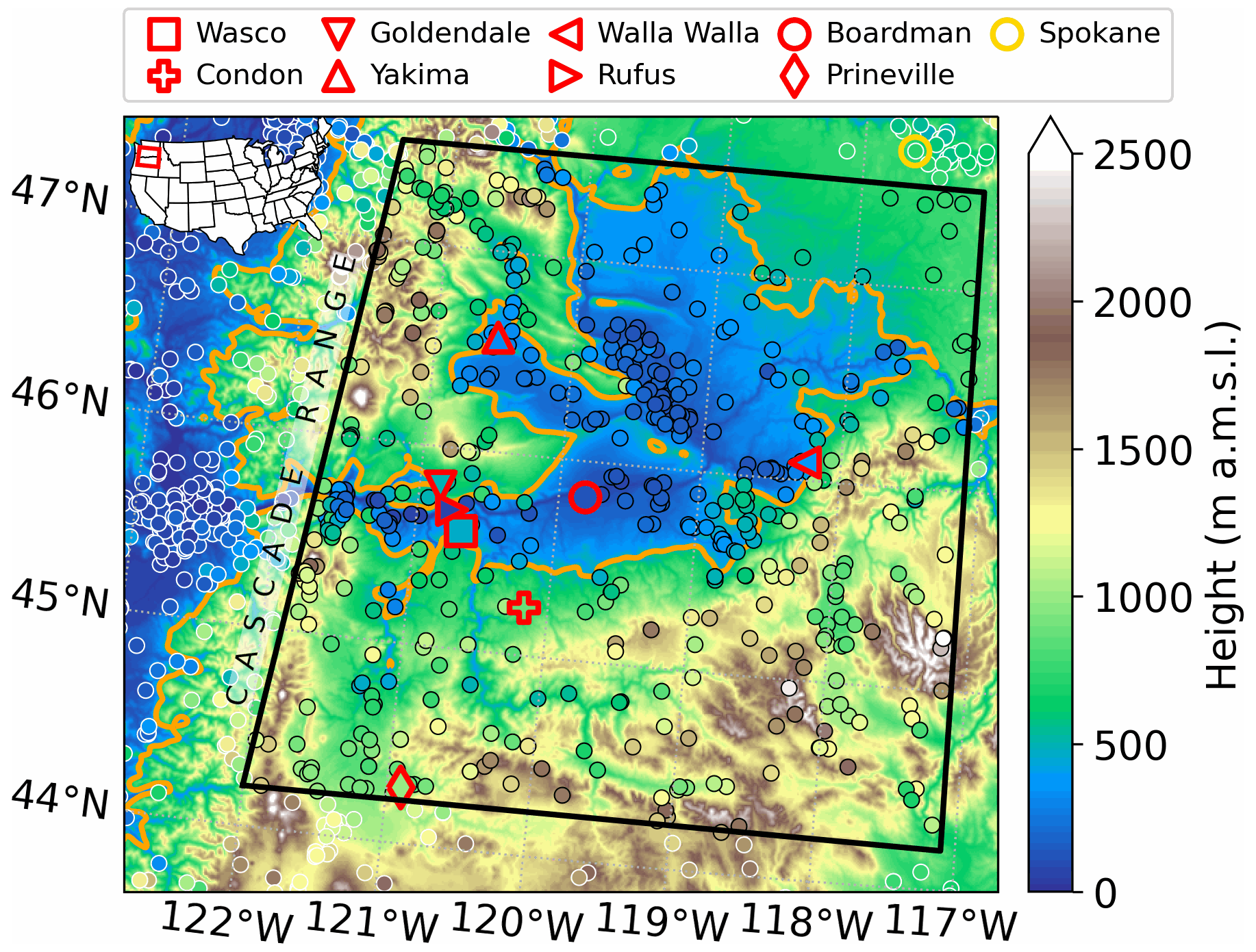
Figure 1Terrain height in the investigation area and location of stations with profile and radiation flux measurements from the WFIP2 campaign (red markers) and from the MesoWest repository (black and white circles). The fill color of each marker indicates the station height. Stations within the black-outlined polygon (red markers and black circles) are used for the model evaluation. The yellow circle indicates the location of the radiosonde station at Spokane. The 500 m terrain contour is given by the orange isoline. Terrain data are from the d02 runs with a 750 m horizontal grid spacing. The inset plot in the upper-left corner shows the location of the investigation area in the United States.
2.1 Observational data
To evaluate the different model runs (Sect. 2.2), we compared the model output to temperature and wind speed profiles retrieved from ground-based remote sensing instruments and in situ near-surface observations. The different observational sources were the same as those used by Adler et al. (2021), and we refer the reader to that publication for a detailed description of the instruments and methods.
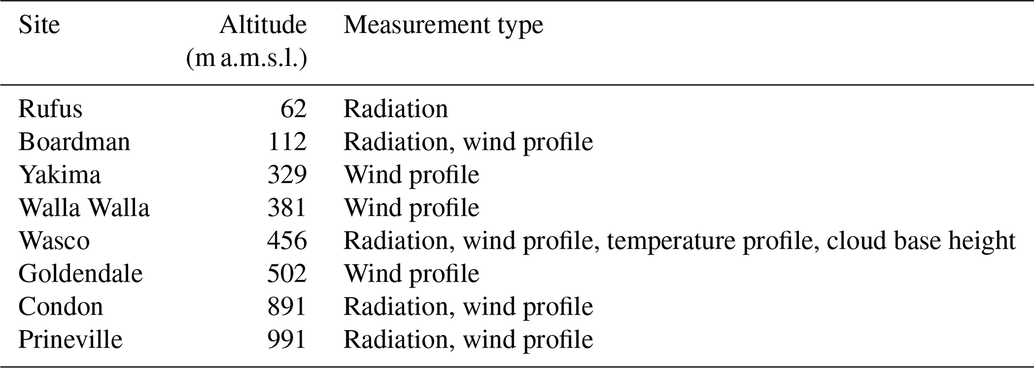
The WFIP2 instrumentation was concentrated in the southern part of the basin with the site at Wasco being the best equipped (Wilczak et al., 2019). Locations of WFIP2 sites are indicated by red markers in Fig. 1, and information on station altitude and measurement types at the different sites are given in Table 1. Seven radar wind profilers were deployed in the basin for WFIP2. They operated at 915 MHz and provided hourly averaged horizontal wind profiles roughly between 100 and 2000 m a.g.l. (above ground level). At Wasco, a microwave radiometer was co-located with a radio acoustic sounding system (RASS) associated with the radar wind profiler. The brightness temperatures measured by the microwave radiometer were combined with the virtual temperature profiles of the RASS and near-surface measurements of temperature and humidity using an optimal estimation physical retrieval (Tropospheric Remotely Observed Profiling via Optimal Estimation – TROPoe; Turner and Löhnert, 2014; Turner and Blumberg, 2019; Turner and Löhnert, 2021) to obtain the best possible information on thermodynamic profiles in the troposphere (Djalalova et al., 2022) as well as the liquid water path (LWP) from these instruments. The output frequency of the TROPoe retrievals was 15 min. Detailed information on the application of the retrieval for the investigated period is given in Adler et al. (2021). As TROPoe uses the optimal estimation framework, it outputs a posterior covariance matrix as a measure of the uncertainty in the retrieval, which includes contributions from uncertainties in the observations, the prior, and the forward model (e.g., Turner and Löhnert, 2021). The 1σ uncertainties of the temperature profiles (i.e., the diagonal elements of the covariance matrix) in our study were less than 1.5 ∘C in the lowest 2.5 km, which are typical values for this instrument combination (Djalalova et al., 2022). The 1σ uncertainty of the retrieved LWP was around 5 kg m−2.
Ceilometer measurements at Wasco provided cloud base height estimates every 16 s, and 15 min averages of shortwave and longwave downward radiation fluxes were available at Rufus, Boardman, Wasco, Condon, and Prineville. Spatial information on shortwave downward radiation flux at the surface was obtained from the Geostationary Operational Environmental Satellites (GOES) Solar Insolation Product (GSIP) with a horizontal grid spacing of 4 km (e.g., Sengupta et al., 2014).
One-hour averages of near-surface temperature measurements were used from a large number of stations distributed in the investigation area (white and black circles in Fig. 1). The data are available through MesoWest, which provides observations from many different organizations (Horel et al., 2002), and can be downloaded with the Mesonet API (Synoptic Data, 2021). The applied quality checks are detailed in Adler et al. (2021). For the model evaluation, more than 500 stations located in the Columbia River basin and the surrounding higher terrain are used (black circles within the black polygon in Fig. 1). Approximately 200 of these stations are located below 500 m a.m.s.l., around 200 are located between 500 and 1250 m a.m.s.l., and nearly 100 stations are located above 1250 m a.m.s.l.
2.2 Model configurations
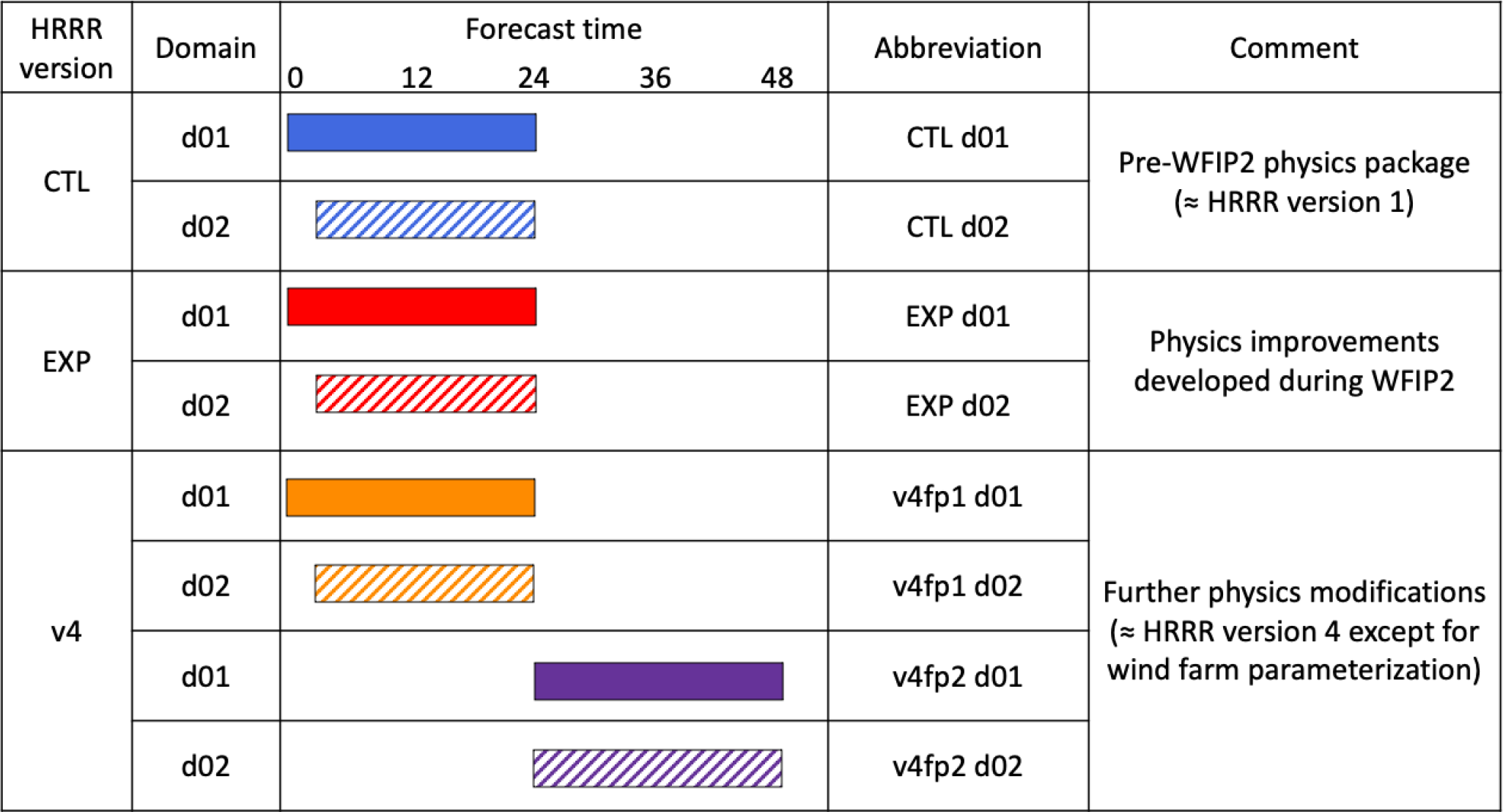
Three versions of the HRRR model and two horizontal grid spacings were evaluated in this study. An overview of the versions, forecast periods, and abbreviations is given in Table 2. The first model version is the WFIP2 control version (hereafter CTL) and corresponds to the configuration of HRRR version 1, which was run operationally at the beginning of WFIP2. The second model version (EXP) uses model developments in physical parameterizations and numerical methods which were targeted in WFIP2. The third model version (v4) is very close to the currently operational HRRR version 4, which encompasses many of the changes present in EXP or refinements of those. Details on WFIP2-specific model changes can be found in Olson et al. (2019a) and Olson et al. (2019b), and details on general HRRR developments can be found in Dowell et al. (2022) and James et al. (2022).
Table 2Overview of the eight model runs used in this study. Three versions of HRRR (CTL, EXP, and v4) are run for two domains with different horizontal grid spacing (d01: Δx=3 km; d02: Δx=750 m). The CTL and EXP runs are 24 h forecasts, and the v4 runs are 48 h forecasts. d01 runs are initialized every 24 h at 00:00 UTC, and nested d02 runs are initialized 3 h later from the 3 h d01 forecast.
The main model developments in EXP and v4 are as follows:
-
The mixing length in the MYNN PBL scheme was revised to improve the forecast performance in stable PBLs and to better maintain inversions. This was accomplished by allowing the mixing length to be independent of height above ground when strong static stability is present and reducing the magnitude of the buoyancy length scale, which is the primary limiting length scale under stable conditions.
-
A mass-flux scheme was included in the MYNN PBL scheme making it an EDMF scheme. This new component represents the nonlocal turbulent transport by thermal plumes in convective PBLs and overall improves the coverage of shallow cumulus and profiles of temperature and humidity. However, during this cold-pool event, the mass-flux scheme was largely inactive, as the surface sensible heat flux was too small to trigger it.
-
A sub-grid-scale cloud representation was implemented that improves the representation of sub-grid-scale stratus and shallow cumulus and also enables the interaction between these clouds and the simulated downward shortwave radiation flux. This has a strong impact on the surface energy balance. There was no sub-grid-scale cloud parameterization in CTL. Changes were made between EXP and v4 to allow more liquid water and smaller effective radii in the sub-grid-scale clouds in the latter. James et al. (2022) attributed an overall reduction in shortwave downward radiation flux bias in v4 when averaging over the continental United States to improvements in the sub-grid-scale cloud scheme.
-
A small-scale gravity wave drag and a form drag due to sub-grid-scale orography was added. The former is active only in stable PBLs and reduces the near-surface wind speed and the shear-generated turbulence, which improves the maintenance of cold pools. Both are only active when the horizontal grid spacing is smaller than 1 km.
-
Horizontal diffusion along terrain-following σ levels was replaced with diffusion in Cartesian space which improves the maintenance of cold pools by no longer mixing vertically when σ levels follow steep terrain.
-
A sixth-order filter was implemented that reduced filtering of scalars and momentum over steep terrain and helped to maintain clouds and cold pools. While this filter was already present in EXP, a lower diffusion parameter was used in v4 that shuts off mixing more aggressively.
Each model version was run for two domains with different horizontal grid spacing. The outer domain encompasses the western United States (Δx=3 km, hereafter referred to as d01). A nested domain was centered on the Columbia River basin with Δx=750 m (hereafter referred to as d02). The domains are shown in Fig. 2 of Olson et al. (2019b). For this study, we used d01 runs which were initialized every 24 h at 00:00 UTC. The model output was written every 15 min. The model was run in a “cold-start” configuration, where initial conditions were supplied from the RAP model without additional data assimilation or antecedent cycling (Olson et al., 2019b). After 3 h of spin-up during which the model atmosphere adjusted to the higher-resolution terrain, the nested d02 runs were initialized from the 3 h d01 forecast. This relatively short spin-up time is possible because the RAP is designed for short-range forecasting and its data assimilation system has a tighter fit to observations than a data assimilation system used for medium-range forecasting (Benjamin et al., 2016). Furthermore, soil state consistency is achieved by using the same land surface model in the RAP and in the HRRR (Dowell et al., 2022). To avoid spin-up effects and to be consistent for the different domains, we only evaluated the model output for times larger than forecast hour 3.
The CTL and EXP runs were not specifically carried out for this study; they were conducted as part of WFIP2 model development efforts (Olson et al., 2019b) and were run for 24 h. The investigated cold-pool event fell within the winter reforecast period (Table 2 of Bianco et al., 2021). Unfortunately, no model output was stored for 18 January for both EXP runs nor for the d02 CTL run. The v4 version was run specifically for this study with the same setup as CTL and EXP for consistency, only the reforecast horizon was extended to 48 h in order to allow an investigation of how the representation of the cold pool may have changed for longer forecast hours. For this purpose, we split the v4 runs into two forecast periods with forecast period 1 (v4fp1) encompassing hours 3–24 and forecast period 2 (v4fp2) encompassing hours 24–48 (Table 2). Note that we only used forecast hours 27–48 for v4fp2 when computing statistics in order to compare the same hours of the day for v4fp1 and v4fp2. To study clouds, additional output variables were added in v4 which included the LWP as well as profiles of cloud water, snow, and ice mixing ratios. The LWP and mixing ratios include contributions from the resolved (grid-scale) and sub-grid-scale clouds.
To compute the differences between the model and the observations, model variables were bilinearly interpolated to the latitude/longitude of the measurement sites, and the temperature and wind simulated profiles were further linearly interpolated to the measurement heights. The temperature profile and radiation flux biases were defined as model data minus observation data and were computed every 15 min. As wind speed profiles and near-surface temperature measurements were available as hourly averages, hourly averaged model data were used for the computation of these biases.
In this section, different characteristics of the cold pool are evaluated for each of the CTL, EXP, and v4fp1 runs (details in Table 2). This includes the analysis of biases between the simulated and observed temperature and wind speed profiles (Sect. 3.2), the temporal evolution of the cold-pool strength (Sect. 3.3), and the dependence of the near-surface temperature biases on station height (Sect. 3.4).
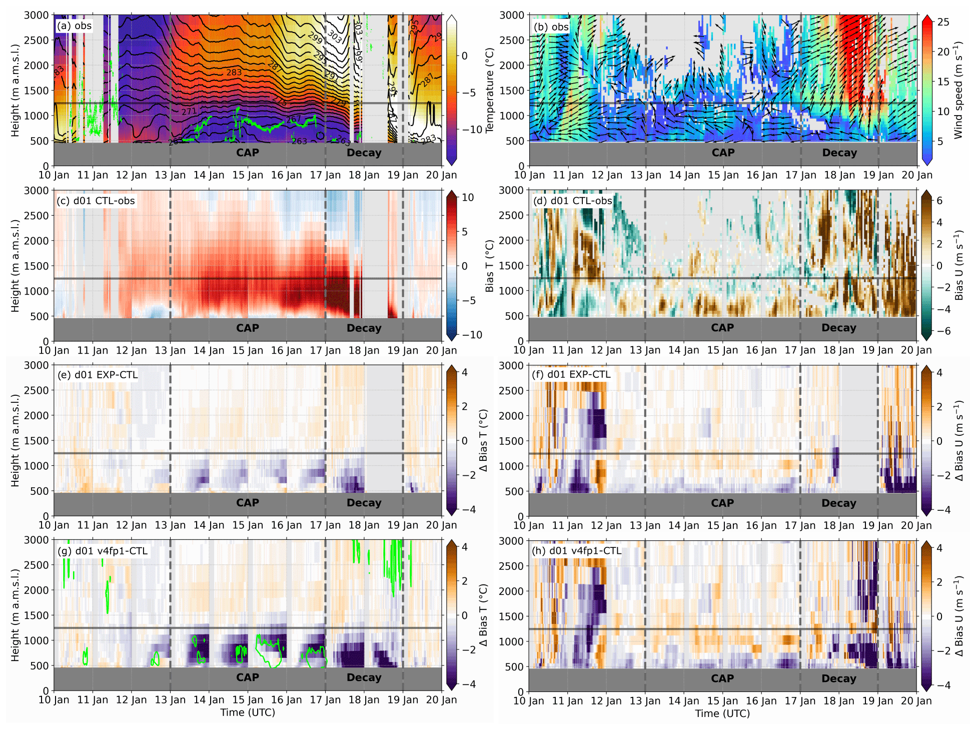
Figure 2Time–height section of observed (a) temperature (color-coded) and potential temperature (isolines) and (b) horizontal wind speed (color-coded) and horizontal wind vector (arrows) at Wasco. Time–height section of (c) temperature (T) bias and (d) horizontal wind speed (U) bias for d01 CTL as well as the changes in (e, g) temperature bias and (f, h) horizontal wind speed bias between EXP and CTL and between v4fp1 and CTL, respectively, at Wasco. The green dots show the observed cloud base height in panel (a), and the green contours show the simulated 0.1 g kg−1 isoline of total condensate (cloud water, snow, and ice mixing ratio) in panel (g). The horizontal gray line indicates the mean ridge height, dark gray shading indicates the station height, and light gray shading indicates missing data. The CAP and Decay periods are indicated by the vertical dashed lines.
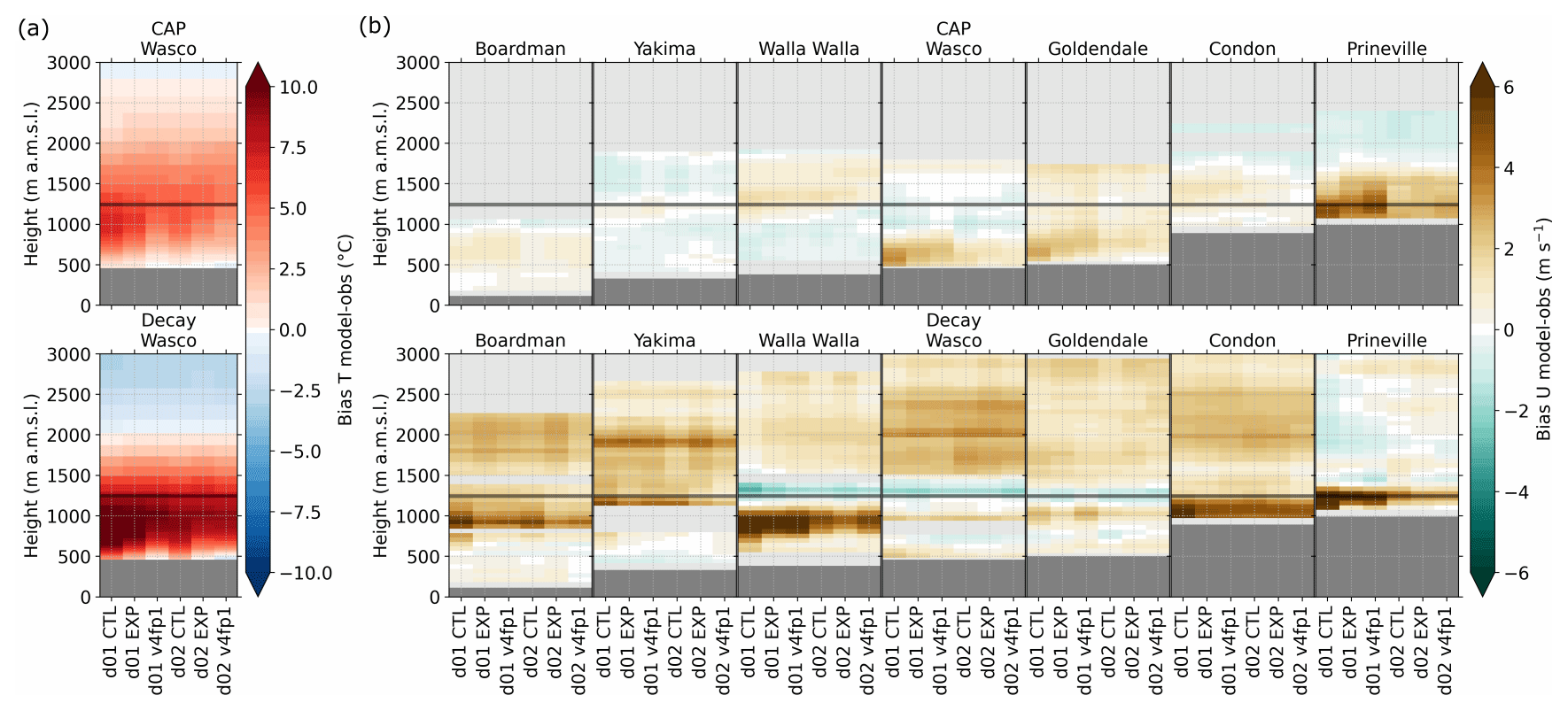
Figure 3Profiles of mean temperature (T) bias (a) and horizontal wind speed (U) bias (b) averaged over the CAP and Decay periods for EXP, CTL, and v4fp1 at different locations in the Columbia River basin. The horizontal gray line indicates the mean ridge height, dark gray shading indicates the station height, and light gray shading indicates missing data.
3.1 Observed temperature and wind profiles
Figure 2a and b illustrate the observed temperature and wind evolution at Wasco during the 10 d period. A detailed description of the temporal evolution of the cold pool and the relevant processes is given in Adler et al. (2021). During the first 3 d, a strong snowstorm passed the area associated with a decrease in temperature and strong northeasterly flow, which was channeled along the west–east valley axis (Fig. 2a, b) and left the ground in the investigation area snow covered during the cold-pool period. Towards the end of 12 January, warming above around 1200 m a.m.s.l., i.e., above the mean ridge height, initiated the formation of the cold pool, which was quickly enhanced by decreasing temperatures in lower layers (Fig. 2a).
From 13 through to 16 January (hereafter referred to as the CAP period), the cold pool was maintained and exhibited a layered structure: the lowest few hundred meters showed a diurnal cycle due to daytime warming and nighttime radiative cooling. Above this layer up to approximately the mean ridge height, the temperature stratification was weakly stable and showed no diurnal cycle. This layer was topped by a strong elevated inversion up to around 2000 m a.m.s.l. Low-level clouds and fog were present during the CAP period, with cloud base heights usually less than 300 m a.g.l., and these impacted the low-level stratification (Fig. 2a). On 15 and 16 January, when cloud base heights were fairly constant and persistent with time, the sub-cloud layer was weakly stably stratified, while a more stable stratification existed on 13 and 14 January when cloud base heights were more variable. Wind within the cold pool was generally weak and easterly (Fig. 2b). We are confident in the accuracy of the retrieved temperature profiles because (i) Adler et al. (2021) found a good agreement with respect to the depth and strength of the temperature inversion between the retrieved free-air profiles and pseudo-vertical profiles derived from the many surface stations in the area and (ii) the differences in low-level stratification during cloudy and cloud-free periods are physically consistent.
With the approach of a low-pressure system from the northwest, strong southwesterly wind and first warm and then cold air reached the area (Fig. 2a, b). A warm front with precipitation passed it on 18 January, which inhibited the retrieval of temperature profiles for much of the day (Fig. 2a). The warm southwesterly flow gradually descended on 17 and 18 January, decreasing the cold-pool depth (Decay period). The gradual warming in the lower layers and cooling in the upper layers eventually eroded the cold pool by 19 January. Adler et al. (2021) found that strong winds and warm air first occurred on the slopes in the southern part of the basin and concluded that mountain waves and downslope winds were involved in the decay.
3.2 Bias of temperature and wind speed profiles
For the model evaluation, we concentrated on two periods, namely the 4 d CAP period and the 2 d Decay period. Figure 2c and d depict the respective temperature and wind speed bias for the CTL run using domain d01 as an example. Figure 2e–f and g–h show the changes in biases between EXP and CTL and between v4fp1 and CTL, respectively. To compute the biases, 21 h of model data (hours 3–24) from each reforecast were used. This resulted in discontinuities in time when the model data shifted from one reforecast run to the next, because each reforecast is initialized independently in a cold-start configuration. During the CAP period, the CTL run had a persistent warm temperature bias of several degrees Celsius up to around 2500 m a.m.s.l. except for the lowest few hundred meters (Fig. 2c). The magnitude of the model bias is much larger than the 1σ uncertainty of the retrieved temperature profiles (Sect. 2.1). Looking at the simulated horizontal temperature distribution above ridge height (not shown), we found a general increase in temperature from east to west in the area. As the warm bias above ridge height already existed at initialization, we assume that it was not related to the simulated physical processes in the cold pool. Interestingly, the model runs did not exhibit any warm biases relative to the operational radio soundings at Salem in the west close to the Pacific coast or at Spokane in the far northeastern part of the basin (yellow marker in Fig. 1), probably because the radiosonde data at these stations were assimilated by the RAP (which provided the initial conditions for these reforecasts). The warm bias in the persistent cold pool was reduced below ridge height by up to 2 ∘C in EXP and by up to 4 ∘C in v4fp1 (Fig. 2e, g). The strongest reduction in v4fp1 occurred when clouds were present. At the beginning of the Decay period the warm bias reached as high as 8 ∘C just below mean ridge height in CTL (Fig. 2c), which again was reduced in EXP and v4fp1. Before the CAP period, especially on 10 January, and after the Decay period on 19 January, the model temperature bias was much smaller (< 2 ∘C).
Table 3Mean temperature and wind speed biases during the CAP and Decay periods averaged up to the mean ridge height. The wind speed biases are an average over all seven stations with wind profile measurements.
The CTL run generally showed a positive wind speed bias of several meters per second (m s−1) up to around 800 m a.m.s.l. and a negative bias above up to the mean ridge height during the CAP period at Wasco (Fig. 2d). The magnitude of both biases was reduced in EXP and v4fp1 (Fig. 2f, h). The bias on 17 January, i.e., the first day of the Decay period, was variable below the mean ridge height and generally positive above (Fig. 2d). On the second day, a mainly positive bias was visible below the mean ridge height in CTL which was reduced in v4fp1 (Fig. 2h).
For a complete comparison of temperature bias at Wasco and wind speed bias at all seven radar wind profiler sites within the Columbia River basin for all six runs, we computed mean biases averaged over the CAP and Decay periods (Fig. 3) and, for a more quantitative assessment, averaged the biases up to mean ridge height (Table 3). Due to missing temperature profiles and missing model output on 18 January, the mean bias for the Decay period was computed for 17 January only. The temperature bias showed a continuous but slight improvement (i) when changing the model version from CTL via EXP to v4 while keeping the horizontal grid spacing the same and (ii) when decreasing the horizontal grid spacing, i.e., from d01 to d02, for each model version (Fig. 3a, Table 3). This is consistent with the results of Arthur et al. (2022), who found a better representation of the CAP with decreased horizontal grid spacing. The warm bias below the mean ridge height during the CAP period resulted from an erroneous representation of the vertical temperature structure in all runs (Fig. 4b). The observed weakly stratified layer up to around the mean ridge height was missing, and the temperature inversion started too close to the surface in the model resembling the typical structure of a cloud-free cold pool with a surface-based inversion and a smooth decrease in stability with height (e.g., Whiteman et al., 2001).
The sign of the bias and the bias improvement for newer model versions (as well as for the runs with finer horizontal grid spacing) was less clear and consistent for wind speed than for temperature on average (Table 3) and varied for the different stations (Fig. 3b). This was partly due to gaps in the observational wind speed data (Fig. 2b) which lead to different sample sizes at different sites. As the sign of the bias at Wasco was mostly positive on 18 January and more variable on 17 January (Fig. 2d), especially below ridge height, we would expect a clearer signal in the mean wind bias on 18 January. However, due to the missing model output on that day for some runs, the mean profiles for the Decay period in Fig. 3b are only computed for 17 January, which might explain the absence of clearer improvements. During the CAP period, the lowest-altitude site (Boardman) had a weak positive bias below approximately 1000 m a.m.s.l. for all runs, whereas Yakima and Walla Walla had a slightly negative bias in the same layer. Wasco and Goldendale, two sites that were fairly close together and located on the slopes in the southern part of the basin (Fig. 1), both showed mainly positive biases which were strongest below around 800 m a.m.s.l. Little improvement in bias with finer grid spacing or newer model version was found for the three lowest stations, whereas the positive bias at Wasco and Goldendale was reduced. Prineville, the highest-altitude site in the south of the CRB, had a strong positive bias in all d01 runs (> 5 m s−1). During the Decay period, all sites had a positive wind speed bias, especially below the mean ridge height. The wind speed bias below the mean ridge height was generally improved with the EXP and v4fp1 versions at all stations, which is most clearly seen at Walla Walla and Prineville. This agrees with the findings by Olson et al. (2019b), who identified a reduction in wind speed bias in the upper part of the cold pool during the decay phase of a different cold-pool case due to the model developments in EXP. Even though the model changes led to a reduction in wind speed bias, all versions still showed a positive bias during the Decay period (Table 3). The positive wind speed and temperature biases indicate that the warm and strong flow still descended too fast into the Columbia River basin, at least on the first day of the decay.
3.3 Cold-pool strength and decay
As a proxy for cold-pool strength, the heat deficit (Q) from the surface (hsfc) up to the mean ridge height (hridge) can be used (Whiteman et al., 1999):
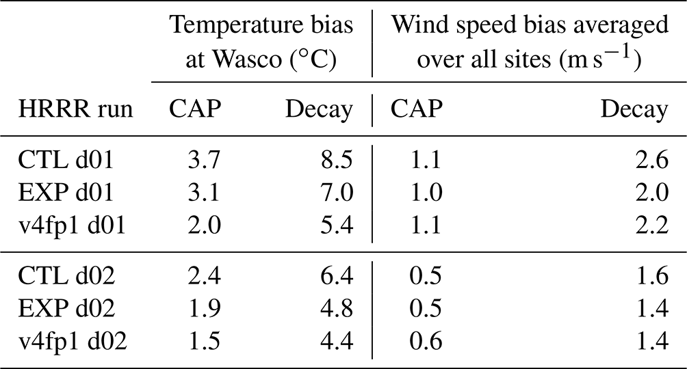
where cp is the specific heat capacity of air at constant pressure, ρ(z) is the air density profile, is the potential temperature at mean ridge height, and θ(z) denotes the potential temperature profile. Figure 4a shows the heat deficit at Wasco for the whole 10 d period computed from observations and model output. With the warming at and above mean ridge height starting on 12 January (Fig. 2a), the heat deficit increased in the observations. This increase was captured by all model versions, likely due to the large-scale character of this warming which was equal in all versions and not impacted by the changes in model physics. All model runs overestimated the heat deficit during the CAP period (Fig. 4a), which is related to the erroneous high value of the ridge height temperature (Fig. 4b). The heat deficit in CTL d01 was lowest and, thus, closest to the observations, but this was not because thermal stratification was most accurate in this run. The overly warm temperature below ridge height rather partly compensated for the warm bias at ridge height (Fig. 4b).
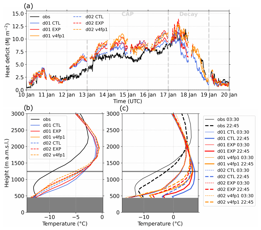
Figure 4(a) Time series of the heat deficit (Eq. 1) and profiles of (b) temperature averaged for the CAP period (13–16 January), and (c) temperature during the Decay period at 03:30 UTC (thin lines) and 22:45 UTC (thick lines) on 17 January at Wasco from observations and the different model runs. The horizontal gray line indicates the mean ridge height, and dark gray shading indicates the station height.
When the warm air descended into the basin on 17 January (Fig. 2a), the cold-pool depth and the associated heat deficit decreased (Fig. 4a). The simulated magnitude of the decrease through the end of 17 January, i.e., until the end of the 24 h forecast period, was stronger than observed, with the strongest decrease found in d01 CTL. This decrease in the heat deficit can easily be understood when comparing temperature profiles at the beginning and end of 17 January (Fig. 4c). The descending warm air resulted in observed warming of up to 4 ∘C above around 750 m a.m.s.l., and daytime convective heating caused warming near the surface of up to 5 ∘C. The simulated temperature profiles were nearly identical in all runs shortly after initialization at 03:30 UTC and were too warm compared with the observations. The impact of the model developments on the cold-pool erosion becomes evident in the following 20 h until 22:45 UTC. Connected to the descending warm air, temperature increased in all runs. The warming was stronger and extended much further downwards in CTL (d01 and d02) and EXP (d01), resulting in a near-surface temperature increase of nearly 15 ∘C in d01 CTL and a substantial weakening of the cold pool, which was well reflected in the low heat deficit values at the end of 17 January (Fig. 4a). Similar to 17 January, the heat deficit decreased on 18 January in the available runs, i.e., d01 CTL, d01 v4fp1, and d02 v4fp1. Albeit still a little too strong compared with the observations, the heat deficit decrease in v4fp1 agreed with the observations much better than in CTL. Even though we found an improvement in the simulated heat deficit during the Decay period, there was still a high bias in wind speed and a warm bias in temperature present (Fig. 3a, b; Table 3), indicating that the cold-pool depth decreased too quickly.
3.4 Dependence of near-surface temperature bias on station height
In the previous sections, we analyzed the vertical temperature structure of the cold pool using profiles at one site in the basin. In the following, we evaluate the dependence of the near-surface temperature bias on station height using the large number of stations in the basin available from the MesoWest repository (station locations in Fig. 1). The stations cover a height range up to 2000 m, and we computed pseudo-vertical profiles by averaging the absolute values and biases at surface stations falling within 100 m height bins. By doing this, any information on horizontal variability was lost, but we found a clear dependence of the bias on station height and less dependence on the location of the station in the basin during the CAP period, which supports the validity of this approach. Pseudo-vertical temperature profiles can be good proxies for free-air temperature within a few degrees during wintertime (Whiteman and Hoch, 2014; Adler et al., 2021). In general, the pseudo-vertical profiles are colder during the night and warmer during the day because of surface cooling and heating.
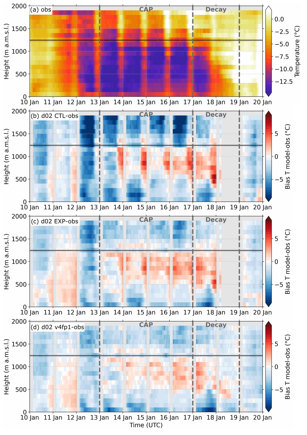
Figure 5Time–height section of (a) observed near-surface temperature and of the temperature (T) bias between d02 (b) CTL, (c) EXP, and (d) v4fp1 and the observed values using data from more than 500 stations distributed in the Columbia River basin (locations in Fig. 1). Values are averaged over 100 m height bins. The horizontal gray line indicates the mean ridge height, and the light gray shading indicates missing data. The CAP and Decay periods are indicated by the vertical dashed lines.
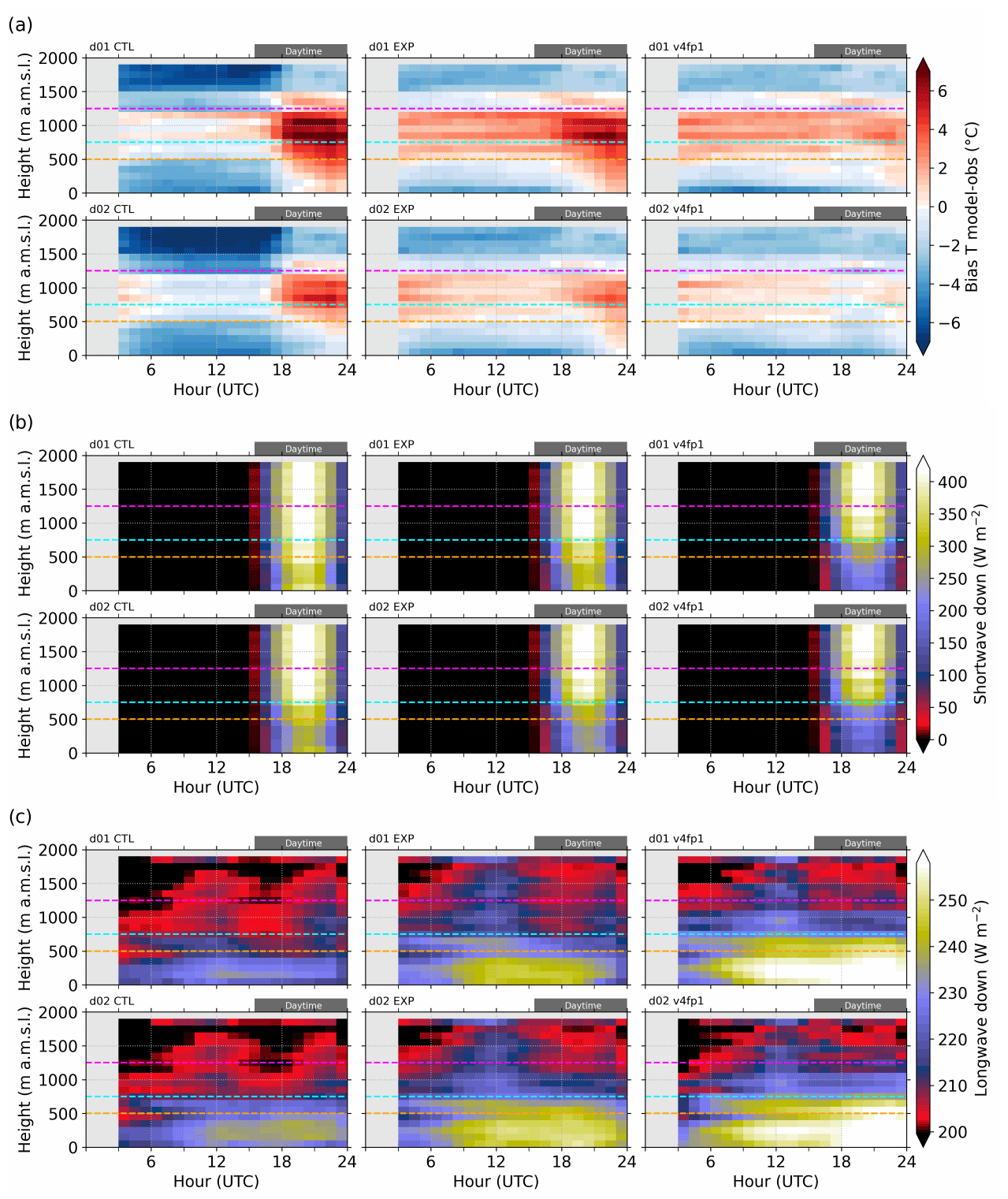
Figure 6Twenty-four-hour composites of (a) near-surface temperature (T) bias, (b) shortwave downward radiation flux, and (c) longwave downward radiation flux averaged over the CAP period (13–16 January). Before calculating the composites, the temperature bias and radiation fluxes are computed at the location of the individual surface stations and then averaged over 100 m height bins. The horizontal dashed lines indicate different height levels with colors corresponding to the terrain contours in Fig. 7.
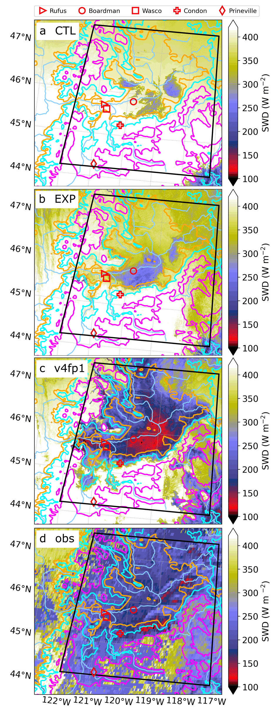
Figure 7Spatial distribution of surface shortwave downward radiation flux (SWD) in d02 (a) CTL, (b) EXP, and (c) v4fp1, and (d) detected by satellite at 21:00 UTC on 14 January. Terrain height contours are indicated by orange (500 m), cyan (750 m), and magenta (1250 m) isolines, and rivers are shown in blue. The red markers indicate the locations of stations with radiation flux measurements.
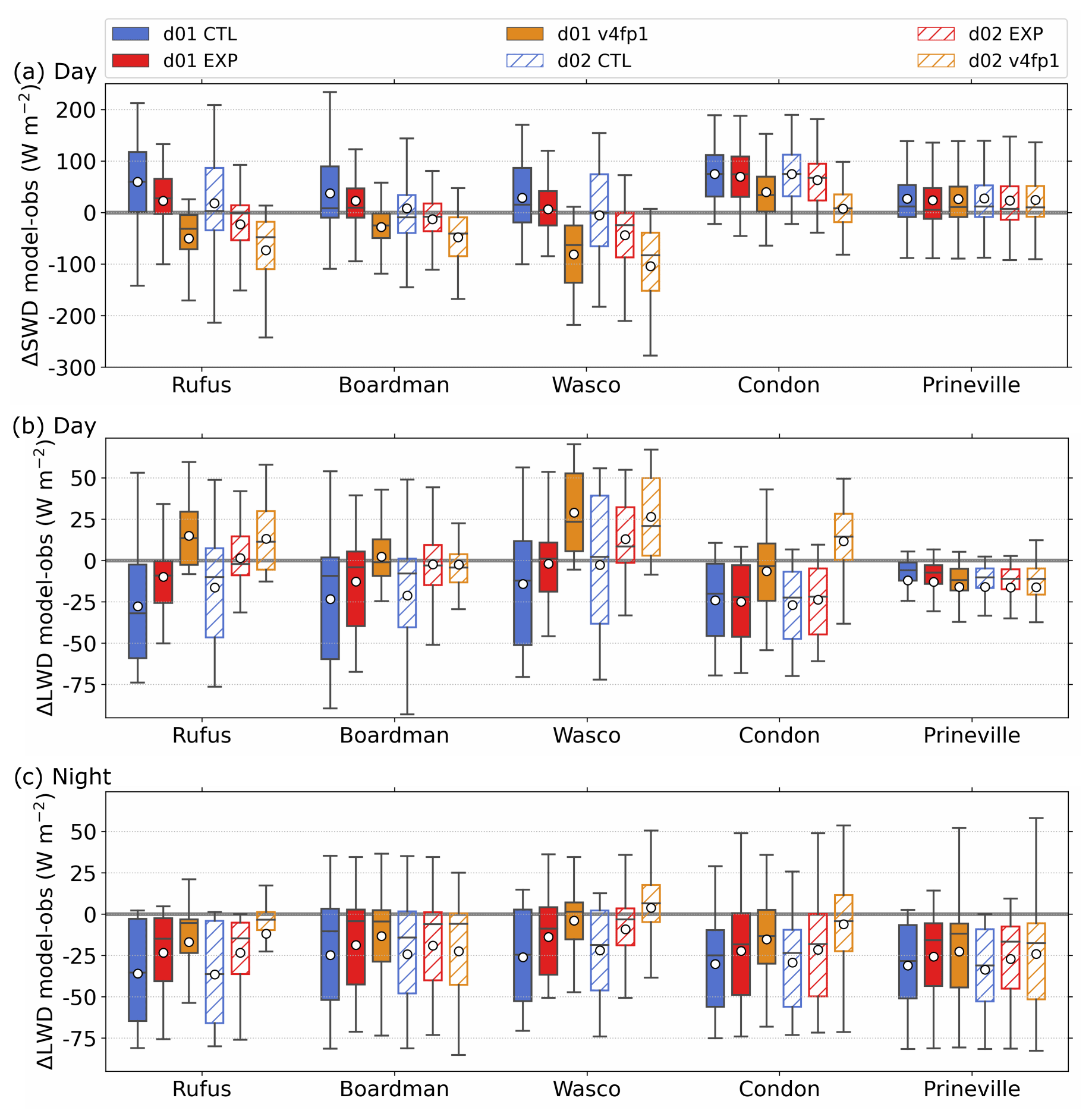
Figure 8Box plot of (a) daytime surface shortwave downward radiation flux bias ΔSWD as well as (b) daytime and (c) nighttime surface longwave downward radiation flux bias ΔLWD between the different model runs (versions: CTL, EXP, v4fp1; domains: d01, d02) and the observations at Rufus, Boardman, Wasco, Condon, and Prineville during the CAP period. The white circles indicate the mean biases, boxes show the interquartile range with the median indicated by the horizontal line, and the whiskers extend to the points that lie within 1.5 times the interquartile range of the lower and upper quartiles.
Figure 5a shows the temporal evolution of the observed pseudo-vertical temperature profiles during the 10 d period. The cold pool was well visible, with cold temperatures at the stations below the mean ridge height and warmer air at stations higher up. A clear diurnal cycle with higher temperatures during the day was evident during the CAP period. The warming during the Decay period first occurred at higher-altitude stations and progressively affected stations at lower altitudes. During the CAP period, the biases were very similar from one day to the other (Fig. 5b, c, d), which makes it suitable to compute 24 h composites by averaging the biases for the 4 d during the CAP period (Fig. 6a). The bias changed its sign with height, and roughly three height layers can be distinguished, 0–500 m a.m.s.l. (Layer 1), 500–1250 m a.m.s.l. (Layer 2), and above 1250 m a.m.s.l. (Layer 3), with generally negative biases in Layers 1 and 3 and a positive bias in Layer 2. In CTL, the negative bias reached values as low as −8 ∘C in Layer 3 and −5 ∘C in Layer 1 during nighttime. A diurnal cycle of the bias was visible in all layers in CTL and somewhat reduced in EXP, but it was much smaller in v4fp1 (Figs. 5b, c, d; 6a). This diurnal cycle was most pronounced in Layer 1 and Layer 2, with a daytime bias regularly exceeding 4 ∘C and even going up to 8 ∘C for d01 CTL (Figs. 5b, 6a).
We suspect that the differences in the temperature bias between the different runs were related to differences in low-level cloud cover. Because the LWP, which contains both the resolved grid-scale and sub-grid-scale cloud water mixing ratio, is only output in v4, we used downward radiation fluxes at the surface as a proxy for clouds. During daytime, clouds lead to a reduction in the shortwave downward radiation flux. The longwave downward radiation flux can be used during day and night. As thermal emission at cloud base primarily contributes to this downward longwave flux, it is generally larger in the presence of low clouds compared with cloud-free conditions when the troposphere is more transparent in the infrared. Shortwave downward radiation flux increased with station height (Fig. 6b), which indicates that stations at lower altitudes experienced more clouds than stations higher up. While this height dependence was generally visible in all runs, it was most pronounced in both v4fp1 runs. This means that more clouds were present in the basin, especially at stations below around 750 m a.m.s.l., in v4fp1 compared with CTL and EXP. This is well visible in the spatial distribution of surface shortwave downward radiation flux shown at 21:00 UTC on 14 January as an example in Fig. 7a–c. Mid- and high-level clouds were mostly absent at this time. The area with reduced shortwave downward radiation flux indicating low-level clouds was confined to a much smaller region in the lower part of the basin in CTL (Fig. 7a) and EXP (Fig. 7b) compared with v4fp1 (Fig. 7c). From all runs, the extent of reduced shortwave downward radiation fluxes in v4fp1 agreed best with the observed values (Fig. 7d), especially over terrain lower than 750 m. Over the higher terrain, all runs, even v4fp1, overestimated shortwave downward radiation fluxes at the surface (i.e., they underestimated cloud coverage).
The station height dependence of longwave downward radiation flux paints a similar picture (Fig. 6c). Higher values in EXP and v4fp1, mainly at stations below around 750 m a.m.s.l., indicate that more clouds were present on average compared with CTL during both day and nighttime. Thus, the very cold nocturnal biases in CTL (Fig. 6a) can be explained by fewer clouds which fostered strong radiative cooling, while more clouds reduced the negative bias in EXP and v4fp1. A lack of clouds during daytime allowed overly strong radiative heating of the surface in CTL compared with the observations, leading to the high positive temperature bias. The warm bias that we see in EXP and v4fp1 in Layer 2 might be related to the warm bias that we see in the profiles at Wasco (Figs. 2c, 3a, 4b). Overly strong radiative cooling due to the lack of clouds may explain why the positive nighttime bias in Layer 2 in EXP and v4fp1 was not present in CTL but was counteracted by cooling.
Adler et al. (2021) found a good agreement between observed early-morning pseudo-vertical and free-air temperature profiles during the CAP period. This seems not always to be the case in the model. While the warm bias in Layer 2 (Fig. 5a) was consistent with the warm bias in the free-air temperature profiles, at least in some versions (Fig. 2c, e, g), the negative bias in near-surface temperature in Layer 3 was the opposite. This means that the near-surface temperature was much lower than the free-air temperature in the model (not shown), whereas they were similar in the observations (Fig. 6 of Adler et al., 2021). One possible explanation for this is that the model had too few clouds above stations in Layer 3, even in v4fp1. Satellite observations analyzed by Adler et al. (2021) (their Fig. 7) and shown in the example in Fig. 7d indicate that clouds also existed over the higher terrain during the CAP period, although they were less extensive than over lower terrain, whereas the high shortwave downward and low longwave downward radiation fluxes in the model in Layer 3 point towards very few clouds in that layer (Fig. 6b, c). Another reason might be that the model has problems with correctly representing the near-surface temperature at higher altitudes where the vegetation category changes from mainly savannas, grasslands, and wetlands to forest, potentially indicating the need for a canopy model which is currently not implemented in HRRR. Note that the ground was snow covered in the simulations and in reality.
We have seen that the differences in radiation fluxes between the model runs are consistent with the differences in temperature bias during the CAP period. The lowest temperature biases in v4fp1 suggest that the downward radiation fluxes in this version agreed best with the observations. To investigate this, we computed shortwave and longwave downward radiation flux biases at five sites – Rufus, Boardman, and Wasco, which are all located in Layer 1, and Condon and Prineville, located in the upper part of Layer 2 (Fig. 8). As the temperature bias depends on the time of the day (Fig. 5a), we distinguished between day and night and computed the shortwave downward radiation flux bias for daytime hours (Fig. 8a) and the longwave downward radiation flux bias for both (Fig. 8b, c). During the day, CTL and EXP had slightly positive biases in shortwave downward radiation flux (Fig. 8a) and, consistent with that, a negative bias in longwave downward radiation flux (Fig. 8b), indicating a lack of clouds. The sign of these biases changed in v4fp1 at stations in Layer 1, most obviously at Rufus and Wasco, indicating too many or overly thick clouds. During nighttime, CTL and EXP had negative longwave downward radiation flux biases at all sites on average, again indicating a lack of clouds (Fig. 8c). An improvement is visible in v4fp1, where the mean and median biases got smaller, especially at Rufus and Wasco. Little differences are visible at Prineville, indicating that clouds did not change much at that site between the different model runs. Combining the findings from shortwave and longwave downward radiation flux biases, we conclude that v4fp1 represented clouds in Layer 1 better during the nighttime (reduced longwave downward radiation flux bias) but had too many or overly thick clouds in Layer 1 during daytime (negative shortwave downward radiation flux bias and positive downward radiation flux bias).
In Sect. 3, we have seen that model developments between the CTL, EXP, and v4 versions lead to a better representation of the cold-pool structure and low-level clouds with a reduced bias in temperature profiles and near-surface temperature during the first 24 h of the forecast. Now, we extend the analysis to 48 h to investigate if and why the cold-pool characteristics change for longer forecast hours, and we take a closer look at the dominant factors taking advantage of the comprehensive output in v4. For the definition of the runs, see Table 2.
4.1 Impact of clouds on temperature profiles during the CAP period
The comparison between the mean temperature bias at Wasco during the CAP period shows a substantial reduction in the positive temperature bias below around 1500 m a.m.s.l. from v4fp1 to v4fp2 (Fig. 9b). The mean temperature profiles for v4fp2 reveal a weakly stratified layer in the lower few hundred meters, which agrees very well with the observations (Fig. 9a). On average, low-level clouds were present mainly up 1250 m a.m.s.l. in the simulations, somewhat higher in d02 v4fp2 (Fig. 9c). This is the same layer in which the strongest changes in temperature bias occurred between both forecast periods (Fig. 9a, b). To illustrate the change in temperature bias with time of the day, we computed 24 h composites of the bias over the 4 d of the CAP period and averaged them up to the mean ridge height, i.e., the layer in which differences were most pronounced (Fig. 9d). Before around 10:00 UTC, the height-averaged temperature bias at Wasco was several degrees Celsius larger in v4fp1 than in v4fp2 (Fig. 9d). This means that the bias was largest during the first 10 forecast hours and decreased with longer forecast times (forecast hours 24–34). Between 10:00 and 24:00 UTC, the bias was more similar for both forecast periods.
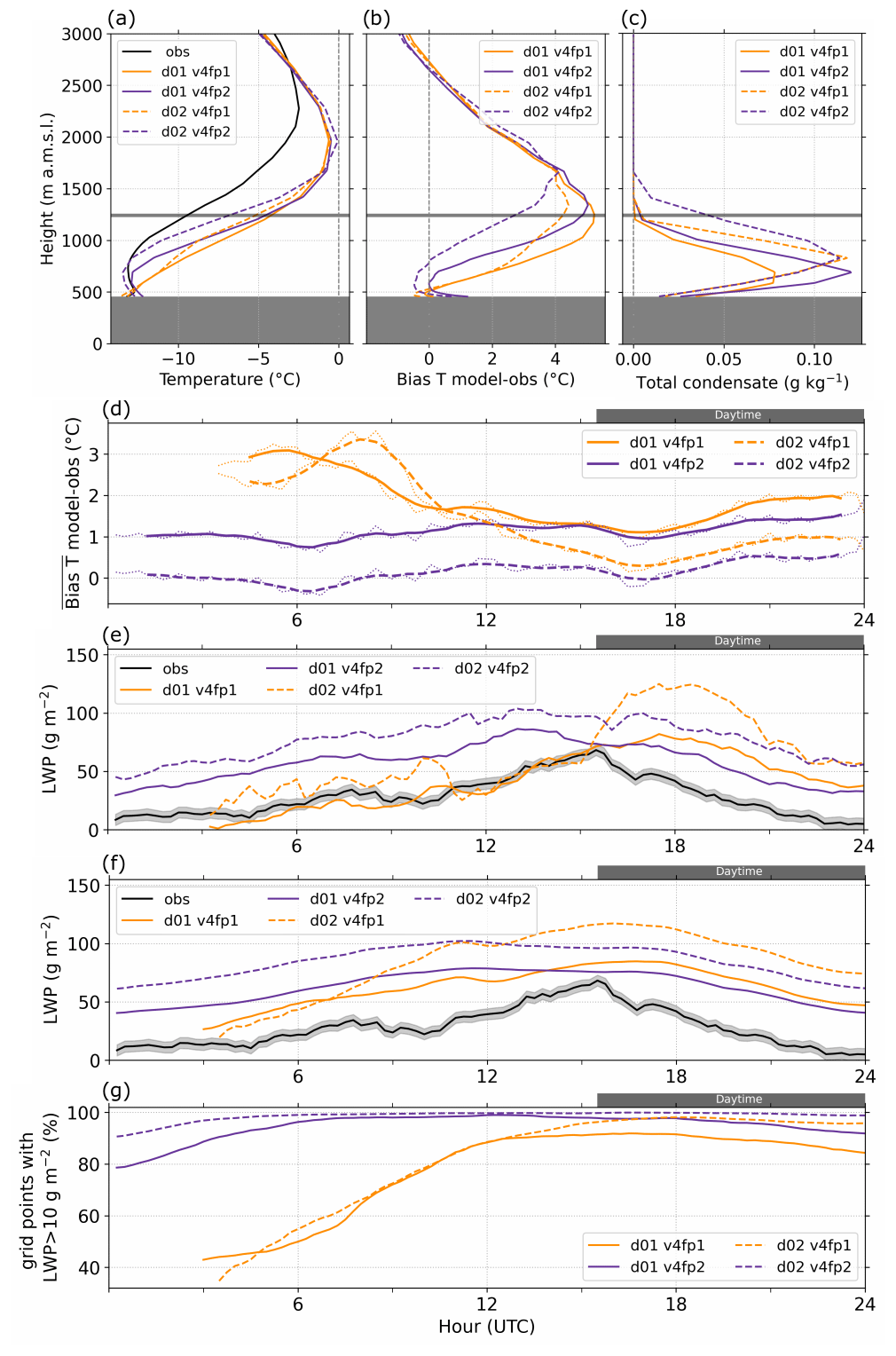
Figure 9Mean profiles of (a) observed and simulated temperature, (b) temperature bias, and (c) simulated total condensate (cloud liquid water, ice, and snow mixing ratio) at Wasco during the CAP period for v4fp1 and v4fp2. The horizontal gray line indicates the mean ridge height, and dark gray shading indicates the station height. Composite time series of (d) temperature bias averaged up to the mean ridge height and (e) the observed and simulated LWP at Wasco; (f) the observed LWP at Wasco and the simulated mean LWP averaged over all grid points in the Columbia River basin; and (g) the percentage of grid points in the basin with LWP > 10 g m−2 during the CAP period. In panel (d), dotted lines show the 15 min output, and solid and dashed lines are smoothed with a 2 h window. Shadings in panels (d) and (e) indicate the 1σ uncertainty of the LWP from the TROPoe retrievals. In panels (e) and (f), only grid points with a terrain height of less than 500 m a.m.s.l. are used.
Because mid- and high-level clouds were largely absent during the CAP period and most of the total condensate was liquid, the LWP very well represented the evolution of the low-level clouds, and we computed 24 h composites of the LWP for the four model runs as well as from observations at Wasco (Fig. 9e). The observed mean LWP at Wasco had a clear diurnal cycle with lower values during the night and maximum values at 15:30 UTC, i.e., at around sunrise (Fig. 9e). During the course of the daytime period, the observed mean LWP decreased and nearly diminished at sunset. Clear differences are visible in the simulated temporal evolution of the LWP for the two forecast periods (Fig. 9e), even though the total condensate profiles had similar maximum values when averaged over time, especially for d02 runs (Fig. 9c). More than 60 % of the simulated LWP originated from the resolved grid-scale clouds on average. The LWP in v4fp1 had a pronounced diurnal cycle with maximum values at around 18:00 UTC. After 18:00 UTC, i.e., during the afternoon, the LWP decreased, as in the observations. The simulated decrease was, however, weaker than observed, which resulted in higher LWP values at sunset at around 24:00 UTC compared with the observations and means that the LWP at the beginning of v4fp2 was too high. The overestimation of the LWP persisted for the whole 24 h period of v4fp2.
The temporal evolution in the LWP can explain the differences in temperature bias between both forecast periods (Fig. 9b). Because clouds were usually missing at model initialization during the CAP period and only slowly formed with time (Fig. 9e, f), the mean temperature structure in v4fp1 (Fig. 9a) resembled a typical cloud-free cold pool with the inversion starting at the surface (e.g., Whiteman et al., 2001). When the clouds thickened and the LWP increased (Fig. 9e), they modified the temperature profiles making them more similar to the observed profiles and reduced the temperature bias in v4fp2 on average (Fig. 9a, b).
The overly weak LWP decrease indicates a failure of the model to clear clouds during daytime due to insufficient mixing either by bottom-up convection or top-down mixing at cloud top. In the MYNN-EDMF scheme used in the v4 simulations, no turbulent mixing at cloud top was present, which could have entrained dry air and helped to erode the more than 500 m deep cloud layer. Wilson and Fovell (2018) tested model changes to the Weather Research and Forecasting (WRF) model to better forecast radiative cold pools and fog in California's Central Valley and found that adding a new cloud top entrainment term to the Yonsei University (YSU) PBL scheme helped to lift and dissolve fog layers. This term is controlled by the fluxes at the PBL top and allowed entrainment to be generated at cloud top by radiative and evaporative cooling. This process is currently not included in the HRRR model.
To investigate the representativeness of the results at Wasco, we averaged the LWP over all grid points in the basin with a terrain height of less than 500 m a.m.s.l. (Fig. 9f). Inspection of the spatial distribution of the LWP (not shown) revealed that the maximum spatial extent of low-level clouds roughly follows the 500 m terrain contour. Thus, the average over these grid points gives a good estimate of the low-level clouds in the basin. The general temporal behavior of the grid-point-averaged LWP was similar to that at Wasco: (i) the LWP was low at the beginning of v4fp1 and increased during the first 15 h after initialization, (ii) the model underestimated the decrease in the LWP during daytime, and (iii) the underestimated decrease in the LWP in v4fp1 during the daytime (i.e., from 15:00 to 24:00 UTC) led to a high LWP in v4fp2. To analyze how extensive the low-level cloud cover in the basin was, we computed the percentage of grid points in the basin with an LWP >10 g m−1 (Fig. 9g). At the beginning of v4fp1, less than 50 % of all grid points in the basin were cloudy. During the subsequent hours, clouds became more widespread, reaching nearly 100 % in d02 at around 18:00 UTC. During v4fp2, nearly all grid points in the basin were cloudy during the whole 24 h, especially in d02.
The small impact of forecast length on temperature and clouds during daytime could be related to the initialization time of the runs at 00:00 UTC. We have seen that cloud cover and the LWP increased in the hours after initialization, i.e., during the night, which resulted in similar values of the LWP during daytime (Fig. 9e, f). If the runs were initialized at 12:00 UTC instead, it is likely that differences in clouds between the two forecast periods would be largest during daytime and less pronounced during nighttime, as the model had more time to generate clouds. However, the investigation of this is beyond the scope of this study. A lack of clouds at initialization, e.g., if they are not inherited at initialization, can lead to unrealistic drops in temperature and the formation of fog layers over snow-covered surfaces at high latitudes as well as the failure of the model to correctly forecast low-level clouds (Hagman et al., 2021). Nevertheless, as low-level clouds formed in the cold pool in the Columbia River basin, albeit slowly, this seems not to be an issue here.
4.2 Dependence of cold-pool decay on forecast length
In Sect. 3.3, we have seen that all model runs captured the timing of the decay of the cold pool on 17 and 18 January fairly well 24 h in advance, although the erosion was too strong, even in the newest model version. Here, we investigate how well the newest model version v4 forecasts the cold-pool decay up to 48 h in advance. Figure 10a shows the heat deficit at Wasco computed with Eq. (1) from the observations and from v4fp1 and v4fp2. At the beginning of the decay period on 17 January, the heat deficit was higher in v4fp2 than in v4fp1 (Fig. 10a). These differences arose from the different temperature profiles (thin lines in Fig. 10b). As a result of the low-level clouds present in the cold pool in v4fp2 (Sect. 4.1), a weakly stratified layer topped by an elevated inversion was present in v4fp2, which was absent in v4fp1. Until the end of the day, descending warm air results in the formation of a strong temperature inversion up to around 1000 m a.m.s.l. which was very similar in both forecast periods (thick lines in Fig. 10b). Differences in the vertical structure were then even larger between runs with different horizontal grid spacing than they were between different forecast periods. This means that, despite the differences in stratification at the beginning of the Decay period, the degree of erosion at the end of the first day was very similar in both forecast periods. This suggests that large-scale forcing was the decisive factor for the cold-pool decay and that the pre-decay stratification did not matter in this case.
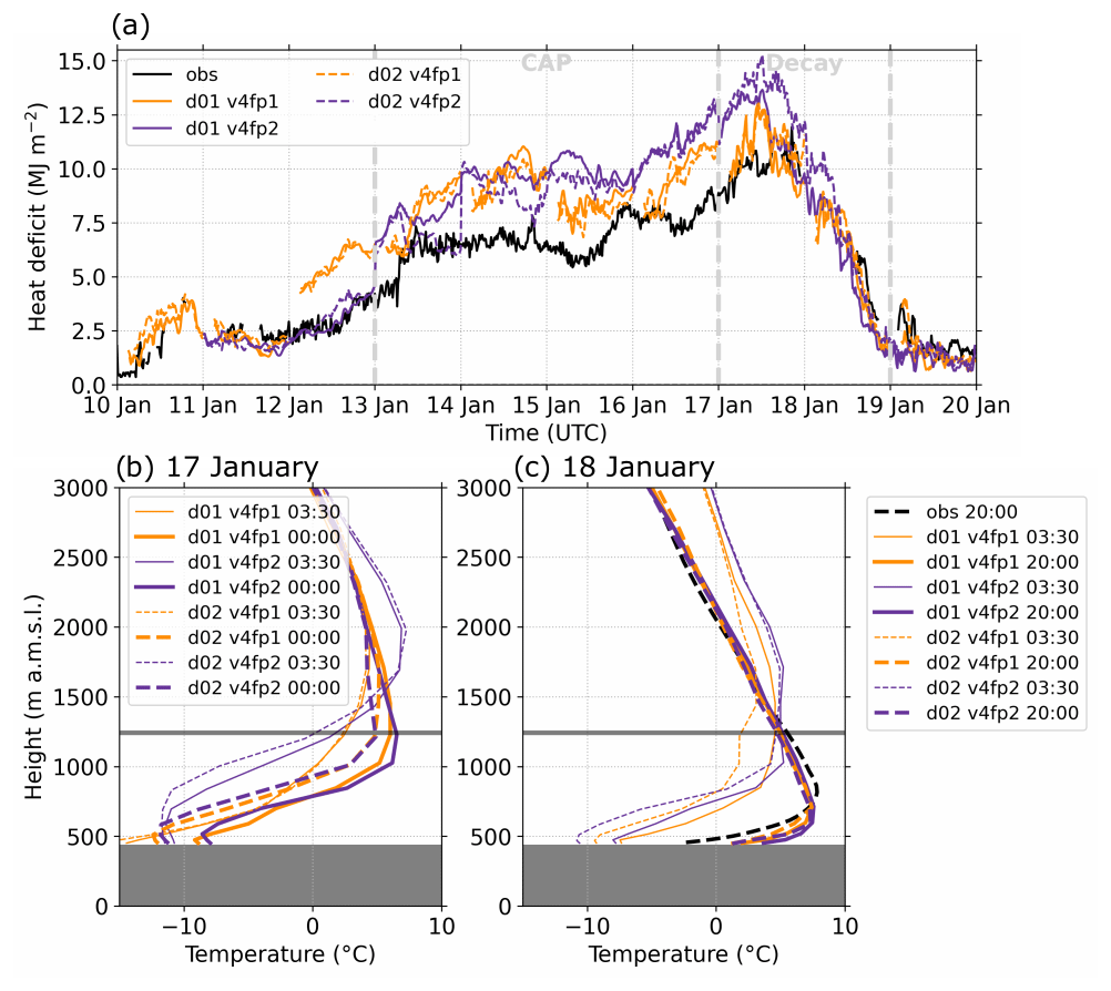
Figure 10(a) Time series of the heat deficit (Eq. 1) from observations and model runs v4fp1 and v4fp2 at Wasco. Profiles of simulated temperature at Wasco during the Decay period on (b) 17 January and (c) on 18 January at the beginning (thin lines) and end (thick lines) of the respective day. In panel (c), the observed temperature profile at 20:00 UTC is added. The horizontal gray line indicates the mean ridge height, and dark gray shading indicates the station height.
On 18 January, the observed and simulated heat deficits for both forecast periods were very similar (Fig. 10a), in agreement with similar temperature profiles (Fig. 10c). However, the heat deficit in all runs was slightly lower than observed at the end of this day, which was reflected in warmer temperatures near the surface and indicates overly fast erosion. Arthur et al. (2022) found that using a 3D PBL scheme instead of the 1D PBL scheme better maintained the temperature structure in the lower few hundred meters on 18 January.
4.3 Impact of clouds on the near-surface temperature bias during the CAP period
At surface stations below around 500 m a.m.s.l. (Layer 1), a cold temperature bias was visible during the CAP period in v4fp1 (Fig. 6a). This cold bias turned into a warm bias in v4fp2, especially during nighttime (Fig. 11a). To understand if this change in the sign of the bias was related to the more extensive clouds during v4fp2 (Fig. 9f, g), we compared the change in temperature to the change in the LWP between the two forecast periods. Figure 11b and c show the relationship between the LWP and temperature differences for individual stations below 500 m for all nighttime hours during the 4 d CAP period. At the majority of stations that detected an increase in temperature from v4fp1 to v4fp2, the LWP also increased (first quadrant in Fig. 11b and c). The relationship between the LWP changes and temperature changes is particularly evident for stations and times when the LWP in v4fp1 was small (red contours in Fig. 11b and c). If the LWP was already large (>50 g m−2) in v4fp1, temperature did not change much between the two forecast periods, probably because the clouds were already opaque in the longwave and, thus, were contributing maximum downward radiation flux in v4fp1. This demonstrates the warming effect that low-level clouds have at the surface during nighttime.
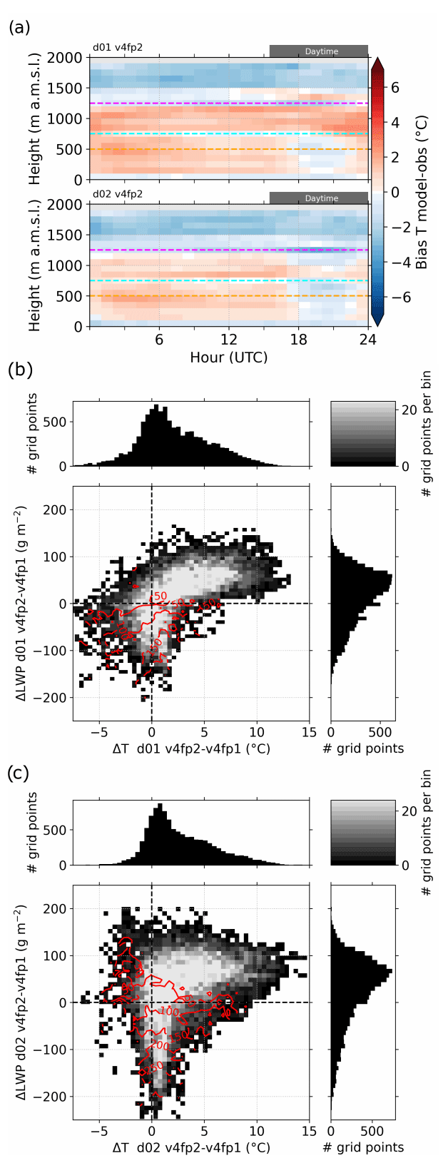
Figure 11(a) Twenty-four-hour composites of near-surface temperature bias averaged over the CAP period (13–16 January) for v4fp2. Before calculating the composites, the temperature bias and radiation fluxes are computed at the location of the individual surface stations and then averaged over 100 m height bins. The horizontal dashed lines indicate different height levels with colors corresponding to terrain contours in Fig. 7. Relationship of the change in liquid water path (ΔLWP) and near-surface temperature (ΔT) between both forecast periods (v4fp2 minus v4fp1) for (b) domain d01 and (c) domain d02. The distributions are computed for surface stations below 500 m a.m.s.l. for all nighttime hours during the CAP period. Red contours indicate the distribution of the LWP in v4fp1.
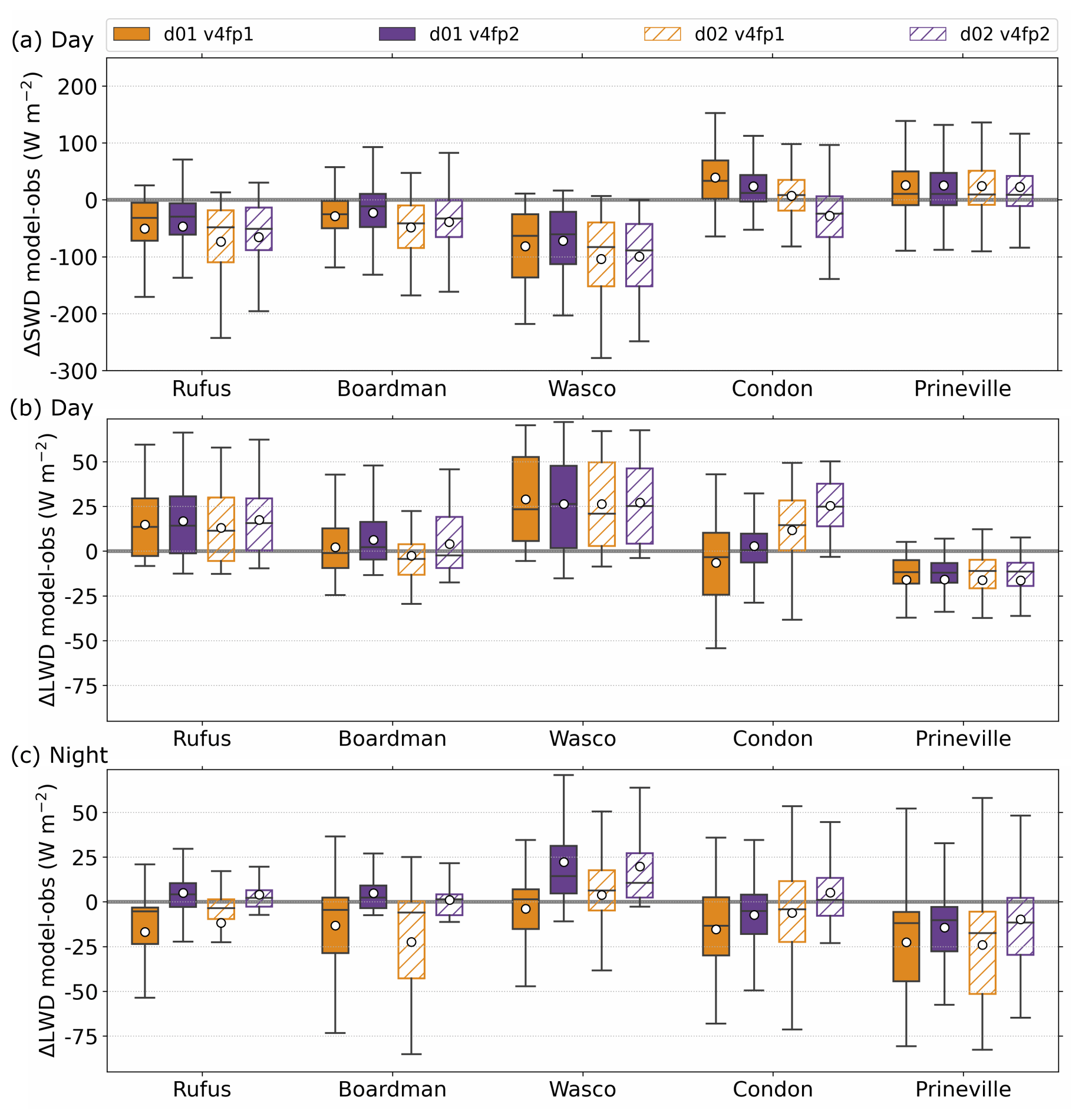
Figure 12Box plot of (a) daytime surface shortwave downward radiation flux bias (ΔSWD) as well as (b) daytime and (c) nighttime surface longwave downward radiation flux bias (ΔLWD) between different model runs (versions: v4fp1, v4fp2; domains: d01, d02) and the observations at Rufus, Boardman, Wasco, Condon, and Prineville during the CAP period. The white circles indicate the mean biases, boxes show the interquartile range with the median indicated by the horizontal line, and the whiskers extend to the points that lie within 1.5 times the interquartile range of the lower and upper quartiles.
The differences in clouds in the lower part of the basin between both forecast periods are consistent with biases in shortwave and longwave downward radiation fluxes during the CAP period (Fig. 12). During daytime, the shortwave downward radiation flux bias was negative and the longwave downward radiation flux bias was positive on average at stations within Layer 1 with differences between both forecast periods being small (Fig. 12a, b), implying that the model had too many clouds regardless of the forecast period. During nighttime, the negative longwave downward radiation flux bias at Rufus and Boardman in v4fp1 was nearly eliminated in v4fp2, while at Wasco a positive bias appeared which was not present in v4fp1 (Fig. 12c). This can be explained by spatial variability in the observed fluxes (and thus clouds) which was not correctly represented in the simulations. The mean observed nighttime longwave downward radiation flux was higher at Rufus and Boardman than at Wasco, indicating more clouds at the lower-altitude stations (Table 1). While the simulated flux at Wasco in v4fp1 agreed fairly well with the observations on average, it was much too low at Boardman, meaning that the model did not capture the higher cloud fraction at Boardman. In v4fp2, the simulated longwave downward radiation flux was high at both sites on average, indicating similar cloud cover in contradiction to the observations. The higher fluxes in v4fp2 better agreed with the observations at Rufus and Boardman, reducing the bias, whereas they overestimated the fluxes at Wasco, causing the positive bias. The warm temperature bias near the surface at stations below 500 m (Fig. 11a) and the widespread clouds (Fig. 9g), high LWP (Fig. 9f), and positive longwave downward radiation flux bias (Fig. 12c) indicate that the extent and thickness of low-level clouds in the basin during nighttime in v4fp2 was overestimated.
In this study, we evaluated three versions of NOAA's HRRR model for two horizontal grid spacings (Δx=750 m and Δx=3 km) for a persistent cold-pool event in the Columbia River basin. For the evaluation, we used remote sensing and in situ observations of temperature, wind, and radiation fluxes gathered during the WFIP2 field campaign as well as near-surface temperature measurements from a large number of stations downloaded from the MesoWest repository. A key component of the WFIP2 project was the model developments in HRRR to improve the forecast for wind energy applications. The three HRRR versions under evaluation were the version that was run operationally at the beginning of WFIP2 (CTL), a version that uses model developments targeted in WFIP2 (EXP), and a version very close to the currently operational HRRR version (v4fp1 and v4fp2). Our aims were to investigate (i) how changes in the model physical parameterizations and numerical methods impacted the cold-pool structure and evolution, in particular temperature and low-level clouds, and (ii) if and how the model performance changed for a longer reforecast horizon.
In a first step, we compared the three versions and two horizontal grid spacings during the 4 d persistent CAP period and the 2 d Decay period. For this we used 24 h reforecasts initialized at 00:00 UTC. The findings of the first step are as follows:
-
Low-level clouds were observed during the CAP period which were associated with a weakly stratified sub-cloud layer at a profiling site at Wasco in the basin. In all model runs, the mean vertical temperature profiles at this site resembled the typical structure of a cloud-free cold pool with a surface-based inversion indicating that clouds were underestimated either in frequency or thickness. This led to a mostly warm bias in the persistent cold pool. During the cold-pool decay, high temperature and high wind speed biases were present, indicating an overly fast top-down erosion of the cold pool. Although present in all versions, the biases were reduced in EXP and v4fp1 compared with CTL. Similarly, the biases were also reduced when the model used smaller horizontal grid spacing (finer resolution).
-
The near-surface temperature bias at more than 500 stations in the Columbia River basin area showed a clear dependence on station height. In contrast to the positive temperature bias through most of the lowest 2.5 km in the free atmosphere, stations below 500 m a.m.s.l. and above the mean ridge height at 1250 m a.m.s.l. showed a negative bias, and stations in between often showed a positive bias. A strong diurnal cycle in the temperature bias occurred in CTL, which was somewhat reduced in EXP and was nearly eliminated in v4fp1. The differences in surface temperature bias between the different model versions were consistent with differences in longwave and shortwave downward radiation fluxes, which we used as a proxy for low-level clouds. Nocturnal longwave downward radiation flux biases were smallest in v4fp1, pointing to more realistic clouds during the night. On the other hand, the radiation flux biases indicated an overestimation of clouds during daytime in the newest model version.
In a second step, we investigated the performance of the newest model version (v4) for longer forecast hours by dividing the 48 h long reforecasts in half and comparing both forecast periods (v4fp1 and v4fp2). The findings of the second step are as follows:
-
Cloud characteristics were fairly similar during the daytime for both forecast periods, while more clouds were present during the night in v4fp2. The difference during the night arose because few clouds were present at model initialization at 00:00 UTC (around sunset) and clouds gradually formed during the first 15 h of the forecast, i.e., during much of the nighttime period of v4fp1, while clouds were already present at sunset and persisted through the night in v4fp2. During daytime, the simulated LWP was high during both forecast periods and decreased less than observed, indicating insufficient clearing of the clouds. The warm bias in the temperature profiles below mean ridge height was much reduced in the lower 500 m during the CAP period in v4fp2, due to the increased presence of low-level clouds and a weakly stratified sub-cloud layer.
-
Despite the differences in clouds and temperature during the CAP period between both forecast periods, the timing of the cold-pool decay was equally well captured in both forecast periods. This indicates that large-scale forcing was decisive for the decay of this cold-pool event and that the pre-decay stratification did not matter.
-
The cold bias at surface stations below 500 m present in v4fp1 during nighttime turned into a warm bias in v4fp2, while differences during daytime were small. This change in the near-surface temperature bias during nighttime was related to an increase in the LWP in v4fp2 at stations that had few clouds (a low LWP) during v4fp1. Consistent with the differences in temperature bias between both forecast periods, differences in the daytime shortwave downward radiation flux bias were small, while a positive longwave downward radiation flux bias occurred during nighttime for v4fp2 at some stations related to overly extensive cloud cover in the simulations.
In short, we found that the model development efforts during WFIP2 and subsequent refinements included in v4 improved the simulation of the cold-pool characteristics, in particular of temperature and clouds. While all model versions were lacking low-level clouds at initialization, clouds gradually formed with time and cloud cover was most realistic in the newest model version. The improved representation of clouds resulted in a reduced near-surface temperature and radiation flux bias as well as a more realistic vertical temperature structure. However, clouds did not clear sufficiently during daytime, leading to an overestimation of clouds during the day and for longer forecast hours which introduced a warm bias near the surface during the second night of the reforecasts.
In this study, we evaluated the model developments as a whole, i.e., we did not investigate the sensitivity to the individual changes in physical parameterizations and numerical methods. Based on our findings and the findings of Olson et al. (2019b) and Berg et al. (2021), we assume that changes in the mixing length, the computation of horizontal diffusion in Cartesian space, the sixth-order filter, the sub-grid-scale clouds, and the small-scale gravity wave drag had an impact, whereas the changes in the mass-flux scheme of the MYNN-EDMF parameterization were less relevant. We found evidence that the overestimation of clouds for longer forecast hours (v4fp2) is related to the failure of the model to sufficiently clear clouds during daytime. HRRR v4 does not include a parameterization of entrainment generated at cloud top by radiative and evaporative cooling. This feature is currently under development. Thus, it is likely that the reduced diffusion in the PBL scheme, the horizontal diffusion, and the sixth-order filter in v4 combine to now undermix under stable conditions, especially without the cloud top cooling mechanism.
All WFIP2 observational data and CTL and EXP model data are available on the U.S. Department of Energy (2020) Data Archive and Portal (https://a2e.energy.gov/data#wfip2). The v4 model data and plotting scripts to produce the figures in this paper are available at Zenodo: https://doi.org/10.5281/zenodo.6713495 (Adler, 2022). The model code used for the CTL and EXP runs is available via https://doi.org/10.5281/zenodo.3369984 (Olson and Kenyon, 2019), and the code used for the v4 runs is available via https://doi.org/10.5281/zenodo.6672455 (Olson, 2022).
BA completed the data analysis and prepared the manuscript with contributions from JMW, LB, IVD, JBO, and DDT. JK conducted the model simulations with HRRR version 4 and IVD assisted with the CTL and EXP model outputs.
The contact author has declared that none of the authors has any competing interests.
Publisher’s note: Copernicus Publications remains neutral with regard to jurisdictional claims in published maps and institutional affiliations.
We thank all of the individuals who helped with WFIP2 site selection, leases, instrument deployment and maintenance, data collection, and data quality control. This research was made possible in part because of the data made available by the governmental agencies, commercial firms, and educational institutions participating in MesoWest. The development of GSIP algorithms and associated products has been supported by the NOAA/NESDIS GOES Product Systems Development and Implementation (G-PSDI) program (Donald Gray, G-PSDI program manager, and Tom Schott, satellite product manager). We further thank the two anonymous reviewers for their helpful comments on the manuscript.
Funding for this work was provided by the U.S. Department of Energy (DOE) Office of Energy Efficiency and Renewable Energy, Wind Energy Technologies Office, and by the NOAA Atmospheric Science for Renewable Energy program. This work was supported by the NOAA cooperative agreements with CIRES (NA17OAR4320101 and NA22OAR4320151) and the NOAA Physical Sciences Laboratory.
This paper was edited by Chiel van Heerwaarden and reviewed by two anonymous referees.
Adler, B.: Selected HRRRv4 model output and plotting scripts for “Evaluation of a cloudy cold-air pool in the Columbia River Basin in different versions of the HRRR model”, Zenodo [data set], https://doi.org/10.5281/zenodo.6713495, 2022. a
Adler, B., Wilczak, J. M., Bianco, L., Djalalova, I., Duncan Jr., J. B., and Turner, D. D.: Observational case study of a persistent cold pool and gap flow in the Columbia River Basin, J. Appl. Meteorol. Clim., 60, 1071–1090, https://doi.org/10.1175/JAMC-D-21-0013.1, 2021. a, b, c, d, e, f, g, h, i, j, k, l, m, n
Arthur, R. S., Juliano, T. W., Adler, B., Krishnamurthy, R., Lundquist, J. K., Kosovic, B., and Jimenez, P. A.: Improved representation of horizontal variability and turbulence in mesoscale simulations of an extended cold-air pool event, J. Appl. Meteorol. Clim., 61, 685–707, https://doi.org/10.1175/JAMC-D-21-0138.1, 2022. a, b, c
Benjamin, S. G., Weygandt, S. S., Brown, J. M., Hu, M., Alexander, C. R., Smirnova, T. G., Olson, J. B., James, E. P., Dowell, D. C., Grell, G. A., Lin, H., Peckham, S. E., Smith, T. L., Moninger, W. R., Kenyon, J. S., and Manikin, G. S.: A North American hourly assimilation and model forecast cycle: The Rapid Refresh, Mon. Weather Rev., 144, 1669–1694, https://doi.org/10.1175/MWR-D-15-0242.1, 2016. a, b
Berg, L. K., Liu, Y., Yang, B., Qian, Y., Krishnamurthy, R., Sheridan, L., and Olson, J.: Time evolution and diurnal variability of the parametric sensitivity of turbine-height winds in the MYNN-EDMF parameterization, J. Geophys. Res., 126, e2020JD034000, https://doi.org/10.1029/2020JD034000, 2021. a, b
Bianco, L., Djalalova, I. V., Wilczak, J. M., Cline, J., Calvert, S., Konopleva-Akish, E., Finley, C., and Freedman, J.: A wind energy ramp tool and metric for measuring the skill of numerical weather prediction models, Weather Forecast., 31, 1137–1156, https://doi.org/10.1175/WAF-D-15-0144.1, 2016. a
Bianco, L., Muradyan, P., Djalalova, I., Wilczak, J., Olson, J., Kenyon, J., Kotamarthi, R., Lantz, K., Long, C., and Turner, D.: Comparison of observations and predictions of daytime planetary-boundary-layer heights and surface meteorological variables in the Columbia River Gorge and Basin during the Second Wind Forecast Improvement Project, Bound.-Lay. Meteorol., 182, 147–172, https://doi.org/10.1007/s10546-021-00645-x, 2021. a
Crosman, E. T. and Horel, J. D.: Large-eddy simulations of a Salt Lake Valley cold-air pool, Atmos. Res., 193, 10–25, https://doi.org/10.1016/j.atmosres.2017.04.010, 2017. a
Djalalova, I. V., Turner, D. D., Bianco, L., Wilczak, J. M., Duncan, J., Adler, B., and Gottas, D.: Improving thermodynamic profile retrievals from microwave radiometers by including radio acoustic sounding system (RASS) observations, Atmos. Meas. Tech., 15, 521–537, https://doi.org/10.5194/amt-15-521-2022, 2022. a, b
Dowell, D. C., Alexander, C. R., James, E. P., Weygandt, S. S., Benjamin, S. G., Manikin, G. S., Blake, B. T., Brown, J. M., Olson, J. B., Hu, M., Smirnova, T. G., Ladwig, T., Kenyon, J. S., Ahmadov, R., Turner, D. D., and Alcott, T. I.: The High-Resolution Rapid Refresh (HRRR): An hourly updating convection-permitting forecast model. Part 1: Motivation and system description, Weather Forecast., 37, 1371–1395, https://doi.org/10.1175/WAF-D-21-0151.1, 2022. a, b, c
Draxl, C., Worsnop, R. P., Xia, G., Pichugina, Y., Chand, D., Lundquist, J. K., Sharp, J., Wedam, G., Wilczak, J. M., and Berg, L. K.: Mountain waves can impact wind power generation, Wind Energ. Sci., 6, 45–60, https://doi.org/10.5194/wes-6-45-2021, 2021. a
Hagman, M., Svensson, G., and Angevine, W.: Forecast of low clouds over a snow surface in the Arctic using the WRF model, Mon. Weather Rev., 149, 2559–2579, https://doi.org/10.1175/MWR-D-20-0396.1, 2021. a
Holtslag, A. A. M., Svensson, G., Baas, P., Basu, S., Beare, B., Beljaars, A. C. M., Bosveld, F. C., Cuxart, J., Lindvall, J., Steeneveld, G. J., Tjernström, M., and Van De Wiel, B. J. H.: Stable atmospheric boundary layers and diurnal cycles: Challenges for weather and climate models, B. Am. Meteorol. Soc., 94, 1691–1706, https://doi.org/10.1175/BAMS-D-11-00187.1, 2013. a
Horel, J., Splitt, M., Dunn, L., Pechmann, J., White, B., Ciliberti, C., Lazarus, S., Slemmer, J., Zaff, D., and Burks, J.: Mesowest: Cooperative mesonets in the western United States, B. Am. Meteorol. Soc., 83, 211–226, https://doi.org/10.1175/1520-0477(2002)083<0211:MCMITW>2.3.CO;2, 2002. a, b
Hughes, J. K., Ross, A. N., Vosper, S. B., Lock, A. P., and Jemmett-Smith, B. C.: Assessment of valley cold pools and clouds in a very high-resolution numerical weather prediction model, Geosci. Model Dev., 8, 3105–3117, https://doi.org/10.5194/gmd-8-3105-2015, 2015. a
James, E. P., Alexander, C. R., Dowell, D. C., Weygandt, S. S., Benjamin, S. G., Manikin, G. S., Brown, J. M., Olson, J. B., Hu, M., Smirnova, T. G., Ladwig, T., Kenyon, J. S., and Turner, D. D.: The High-Resolution Rapid Refresh (HRRR): An hourly updating convection-allowing forecast model. Part 2: Forecast performance, Weather Forecast., 37, 1397–1417, https://doi.org/10.1175/WAF-D-21-0130.1, 2022. a, b
Lareau, N. P. and Horel, J. D.: Turbulent erosion of persistent cold-air pools: Numerical simulations, J. Atmos. Sci., 72, 1409–1427, https://doi.org/10.1175/JAS-D-14-0173.s1, 2015. a
Lareau, N. P., Crosman, E., Whiteman, C. D., Horel, J. D., Hoch, S. W., Brown, W. O., and Horst, T. W.: The persistent cold-air pool study, B. Am. Meteorol. Soc., 94, 51–63, https://doi.org/10.1175/BAMS-D-11-00255.1, 2013. a
Lu, W. and Zhong, S.: A numerical study of a persistent cold air pool episode in the Salt Lake Valley, Utah, J. Geophys. Res., 119, 1733–1752, https://doi.org/10.1002/2013JD020410, 2014. a
McCaffrey, K., Wilczak, J. M., Bianco, L., Grimit, E., Sharp, J., Banta, R., Friedrich, K., Fernando, H., Krishnamurthy, R., Leo, L. S., and Paytsar, M.: Identification and characterization of persistent cold pool events from temperature and wind profilers in the Columbia River Basin, J. Appl. Meteorol. Clim., 58, 2533–2551, https://doi.org/10.1175/JAMC-D-19-0046.1, 2019. a
Neemann, E. M., Crosman, E. T., Horel, J. D., and Avey, L.: Simulations of a cold-air pool associated with elevated wintertime ozone in the Uintah Basin, Utah, Atmos. Chem. Phys., 15, 135–151, https://doi.org/10.5194/acp-15-135-2015, 2015. a, b
Neiman, P. J., Gottas, D. J., and White, A. B.: A two-cool-season wind profiler–based analysis of westward-directed gap flow through the Columbia River Gorge, Mon. Weather Rev., 147, 4653–4680, https://doi.org/10.1175/MWR-D-19-0026.1, 2019. a
Olson, J.: joeolson42/WRFv3.9_HRRRv4: WRFv3.9_HRRRv4 (final_HRRR_code), Zenodo [code], https://doi.org/10.5281/zenodo.6672455, 2022. a
Olson, J. and Kenyon, J.: joeolson42/WFIP2: WFIP2 Experimental HRRR version 1.0 (EXPv1.0), Zenodo [code], https://doi.org/10.5281/zenodo.3369984, 2019. a
Olson, J. B., Kenyon, J. S., Angevine, W. A., Brown, J. M., Pagowski, M., and Sušelj, K.: A description of the MYNN-EDMF Scheme and the coupling to other components in WRF–ARW, NOAA Technical Memorandum OAR GSD, 61, https://doi.org/10.25923/n9wm-be49, 2019a. a
Olson, J. B., Kenyon, J. S., Djalalova, I., Bianco, L., Turner, D. D., Pichugina, Y., Choukulkar, A., Toy, M. D., Brown, J. M., Angevine, W. M., Akish, E., Bao, J., Jimenez, P., Kosovic, B., Lundquist, K. A., Draxl, C., Lundquist, J. K., McCaa, J., McCaffrey, K., Lantz, K., Long, C., Wilczak, J., Banta, R., Marquis, M., Redfern, S., Berg, L. K., Shaw, W., and Cline, J.: Improving wind energy forecasting through numerical weather prediction model development, B. Am. Meteorol. Soc., 100, 2201–2220, https://doi.org/10.1175/BAMS-D-18-0040.1, 2019b. a, b, c, d, e, f, g, h, i, j
Reeves, H. D., Elmore, K. L., Manikin, G. S., and Stensrud, D. J.: Assessment of forecasts during persistent valley cold pools in the Bonneville Basin by the North American Mesoscale Model, Weather Forecast., 26, 447–467, https://doi.org/10.1175/WAF-D-10-05014.1, 2011. a
Sengupta, M., Habte, A., Gotseff, P., Weekley, A., Lopez, A., Anderberg, M., Molling, C., and Heidinger, A.: Physics-based GOES product for use in NREL's national solar radiation database: Preprint, Solar 2014, 6–10 July 2014, San Francisco, California, https://www.osti.gov/biblio/1351563 (last access: 11 August 2020), 2014. a
Shaw, W. J., Berg, L. K., Cline, J., Draxl, C., Djalalova, I., Grimit, E. P., Lundquist, J. K., Marquis, M., McCaa, J., Olson, J. B., Sivaraman, C., Sharp, J., and Wilczak, J. M.: The Second Wind Forecast Improvement Project (WFIP2): general overview, B. Am. Meteorol. Soc., 100, 1687–1699, https://doi.org/10.1175/BAMS-D-18-0036.1, 2019. a
Sun, X. and Holmes, H. A.: Surface turbulent fluxes during persistent cold-air pool events in the Salt Lake Valley, Utah. Part I: observations, J. Appl. Meteorol. Clim., 58, 2553–2568, https://doi.org/10.1175/JAMC-D-19-0053.1, 2019. a
Synoptic Data: Mesonet API, https://developers.synopticdata.com/mesonet/, last access: 6 April 2021. a
Turner, D. D. and Blumberg, W. G.: Improvements to the AERIoe thermodynamic profile retrieval algorithm, IEEE J. Sel. Top. Appl., 12, 1339–1354, https://doi.org/10.1109/JSTARS.2018.2874968, 2019. a
Turner, D. D. and Löhnert, U.: Information content and uncertainties in thermodynamic profiles and liquid cloud properties retrieved from the ground-based atmospheric emitted radiance interferometer (AERI), J. Appl. Meteorol. Clim., 53, 752–771, https://doi.org/10.1175/JAMC-D-13-0126.1, 2014. a
Turner, D. D. and Löhnert, U.: Ground-based temperature and humidity profiling: combining active and passive remote sensors, Atmos. Meas. Tech., 14, 3033–3048, https://doi.org/10.5194/amt-14-3033-2021, 2021. a, b
U.S. Department of Energy: Atmosphere to Electrons: Second Wind Forecast Improvement Project (WFIP2), U.S. Department of Energy [data set], https://a2e.energy.gov/data#wfip2, last access: 8 July 2020. a
VanReken, T. M., Dhammapala, R. S., Jobson, B. T., Bottenus, C. L., VanderSchelden, G. S., Kaspari, S. D., Gao, Z., Zhu, Q., Lamb, B. K., Liu, H., and Johnston, J.: Role of persistent low-level clouds in mitigating air quality impacts of wintertime cold pool conditions, Atmos. Environ., 154, 236–246, https://doi.org/10.1016/j.atmosenv.2017.01.043, 2017. a
Wei, L., Pu, Z., and Wang, S.: Numerical simulation of the life cycle of a persistent wintertime inversion over Salt Lake City, Bound.-Lay. Meteorol., 148, 399–418, https://doi.org/10.1007/s10546-013-9821-2, 2013. a
Whiteman, C. D. and Hoch, S. W.: Pseudovertical temperature profiles in a broad valley from lines of temperature sensors on sidewalls, J. Appl. Meteorol. Clim., 53, 2430–2437, https://doi.org/10.1175/JAMC-D-14-0177.1, 2014. a
Whiteman, C. D., Bian, X., and Zhong, S.: Wintertime evolution of the temperature inversion in the Colorado Plateau Basin, J. Appl. Meteorol., 38, 1103–1117, https://doi.org/10.1175/1520-0450(1999)038<1103:WEOTTI>2.0.CO;2, 1999. a
Whiteman, C. D., Zhong, S., Shaw, W. J., Hubbe, J. M., Bian, X., and Mittelstadt, J.: Cold pools in the Columbia Basin, Weather Forecast., 16, 432–447, https://doi.org/10.1175/1520-0434(2001)016<0432:CPITCB>2.0.CO;2, 2001. a, b, c, d
Wilczak, J. M., Stoelinga, M., Berg, L. K., Sharp, J., Draxl, C., McCaffrey, K., Banta, R. M., Bianco, L., Djalalova, I., Lundquist, J. K., Muradyan, P., Choukulkar, A., Leo, L., Bonin, T., Pichugina, Y., Eckman, R., Long, C. N., Lantz, K., Worsnop, R. P., Bickford, J., Bodini, N., Chand, D., Clifton, A., Cline, J., Cook, D. R., Fernando, H. J. S., Friedrich, K., Krishnamurthy, R., Marquis, M., McCaa, J., Olson, J. B., Otarola-Bustos, S., Scott, G., Shaw, W. J., Wharton, S., and White, A. B.: The Second Wind Forecast Improvement Project (WFIP2): Observational field campaign, B. Am. Meteorol. Soc., 100, 1701–1723, https://doi.org/10.1175/BAMS-D-18-0035.1, 2019. a, b, c, d, e
Wilson, T. H. and Fovell, R. G.: Modeling the evolution and life cycle of radiative cold pools and fog, Weather Forecast., 33, 203–220, https://doi.org/10.1175/WAF-D-17-0109.1, 2018. a
Zhong, S., Whiteman, C. D., Bian, X., Shaw, W. J., and Hubbe, J. M.: Meteorological processes affecting the evolution of a wintertime cold air pool in the Columbia basin, Mon. Weather Rev., 129, 2600–2613, https://doi.org/10.1175/1520-0493(2001)129<2600:MPATEO>2.0.CO;2, 2001. a, b
- Abstract
- Introduction
- Investigation area, observational data, and model configurations
- Evaluation of three HRRR versions
- Cold-pool characteristics for a 48 h forecast horizon in v4
- Summary and conclusions
- Code and data availability
- Author contributions
- Competing interests
- Disclaimer
- Acknowledgements
- Financial support
- Review statement
- References