Representing the impact of Rhizophora mangroves on flow in a hydrodynamic model (COAWST_rh v1.0): the importance of three-dimensional root system structures

Coastal wetland vegetation modulates water flow by exerting drag, which has important implications for sediment transport and geomorphic dynamics. This vegetation effect on flow is commonly represented in hydrodynamic models by approximating the vegetation as an array of vertical cylinders or increased bed roughness. However, this simple approximation may not be valid in the case of Rhizophora mangroves that have complicated three-dimensional root structures. Here, we present a new model to represent the impact of Rhizophora mangroves on flow in hydrodynamic models. The model explicitly accounts for the effects of the three-dimensional root structures on mean flow and turbulence as well as for the effects of two different length scales of vegetation-generated turbulence characterized by stem diameter and root diameter. The model employs an empirical model for the Rhizophora root structures that can be applied using basic vegetation parameters (mean stem diameter and tree density) without rigorous measurements of the root structures. We tested the model against the flows measured by previous studies in a model mangrove forest in the laboratory and an actual mangrove forest in the field, respectively. We show that, compared with the conventional approximation using an array of cylinders or increased bed roughness, the new model significantly improves the predictability of velocity, turbulent kinetic energy, and bed shear stress in Rhizophora mangrove forests. Overall, the presented new model offers a more realistic but feasible framework for simulating flows in Rhizophora mangrove forests with complex root structures using hydrodynamic models.

1 Introduction

Mangroves are one of the coastal wetland habitats that grow in intertidal areas in tropical and subtropical regions (Hamilton and Casey, 2016). They have characteristic aboveground root systems with varying morphological structures among genera, such as the pneumatophores or “pencil roots” of Avicennia and Sonneratia and the prop roots of Rhizophora (Krauss et al., 2014). Due to the presence of these aboveground root systems, mangroves exert drag against water flow that lowers the flow velocity. This creates conditions preferable for the deposition and retention of tidally and fluvially transported sediments (Furukawa et al., 1997; Krauss et al., 2003; Horstman et al., 2015; Chen et al., 2016, 2018; Willemsen et al., 2016; Best et al., 2022), similar to other wetland habitats such as salt marshes (Temmerman et al., 2005; Bouma et al., 2007; Mudd et al., 2010; Weisscher et al., 2022). Flow–vegetation interactions coupled with sediment transport play a major role in driving the long-term geomorphic evolution of wetland habitats (Mariotti and Fagherazzi, 2010; Mariotti and Canestrelli, 2017; Brückner et al., 2019; Kalra et al., 2022; Willemsen et al., 2022). This further determines the persistence of mangroves amidst threats due to sea-level rise (Fagherazzi et al., 2012, 2020; Lovelock et al., 2015; Kirwan et al., 2016).

Representing the effect of vegetation on flow (vegetation drag) in hydrodynamic models is important to advance our understanding of hydrodynamics in coastal wetlands with implications for sediment transport and geomorphic dynamics (Temmerman et al., 2005; Nardin et al., 2016; Lokhorst et al., 2018). Several modeling studies have shown that geomorphic evolution, and, correspondingly, the ecosystems' fate in response to sea-level rise, can vary dramatically depending on the magnitude of vegetation drag (Boechat Albernaz et al., 2020; Xie et al., 2020). The vegetation drag in salt marshes and seagrass beds is commonly represented in hydrodynamic models by an array of vertical cylinders (cylinder drag model; Ashall et al., 2016; Zhu et al., 2021), the drag effect of which has been well studied for both emergent and submerged cases (e.g., Nepf, 1999, 2012). Although fewer compared with studies on salt marshes, some studies have incorporated the drag effects of mangroves in hydrodynamic models to evaluate their role in controlling flow and sediment transport (van Maanen et al., 2015; Bryan et al., 2017; Mullarney et al., 2017; Rodríguez et al., 2017; Xie et al., 2020); however, most work has been limited to Avicennia- or Sonneratia-dominated mangrove forests whose aboveground roots (pencil roots) are geometrically simple and resemble a vertical cylinder array.

In contrast, the root system of the Rhizophora genus (prop root system) has three-dimensionally complicated structures that cannot simply be approximated by an array of vertical cylinders. Consequently, the representation of drag from Rhizophora mangroves in hydrodynamic models remains to be established, despite the global distribution of this mangrove genus (Friess et al., 2019). This knowledge gap can be seen in studies that have approximated drag from Rhizophora mangroves using arbitrarily increased bed roughness (Zhang et al., 2012) or cylinder arrays with an arbitrary cylinder density (Xie et al., 2020) without much theoretical or experimental support (reviewed in Le Minor et al., 2021). One exception is a modeling study by Horstman et al. (2015) that approximated the root structures of Rhizophora mangroves using a cylinder array with vertically variable cylinder densities. However, their method requires an exhausting field survey of the root structures as a requirement for proper model application, which may not be feasible for a forest-scale simulation.

In addition to flow velocity, vegetation affects turbulence (Nepf, 2012; Xu and Nepf, 2020), which is also relevant for the transport of substances (e.g., sediment and solutes) via turbulent diffusion (Tanino and Nepf, 2008; Xu and Nepf, 2021). While several hydrodynamic models can account for vegetation-generated turbulence (e.g., Temmerman et al., 2005; Marsooli et al., 2016), no model has thus far been established to predict the turbulence structures in Rhizophora mangrove forests. Therefore, a rigorous but feasible representation of the impact of Rhizophora mangroves on flow velocity and turbulence in a hydrodynamic model is needed.

One of the challenges of modeling the flow in Rhizophora mangroves is the quantification of the complex root structures, which can be a labor-intensive process when applied at the forest scale. Recently, an empirical model to predict the structures of Rhizophora root systems from the stem diameter was proposed by Yoshikai et al. (2021). The model's general applicability to the root structures of various tree sizes has been extensively confirmed (Yoshikai et al., 2021). This empirical Rhizophora root model (hereafter denoted as the Rh-root model) offers the possibility to feasibly simulate flow at the forest scale once it is implemented in the hydrodynamic model.

In this work, in order to contribute to realistic but feasible simulations of hydrodynamics in Rhizophora mangrove forests, we implement a new drag and turbulence model coupled with the Rh-root model to represent the impacts of Rhizophora mangroves in a three-dimensional hydrodynamic model: the Regional Ocean Modeling System (ROMS; Shchepetkin and McWilliams, 2005) of the Coupled Ocean–Atmosphere–Wave–Sediment Transport (COAWST; Warner et al., 2010) model framework. The impact of the vertically varying projected area of roots on flow velocity and turbulence is specifically taken into consideration by the new model. Furthermore, the new model accounts for two different length scales of turbulence generated by Rhizophora mangroves – stem diameter and root diameter – as characterized using a flume experiment by Maza et al. (2017). Here, we aim to examine the following:

• a.

  How does the consideration of the three-dimensional root structures of Rhizophora mangroves in the hydrodynamic model improve the predictability of flow velocity and turbulence compared with the conventional drag approximation using cylinder arrays or increased bed roughness?

• b.

  How can the new model be effectively applied to Rhizophora mangrove forests in the field with limited known root parameters?

2 Materials and methods

2.1 Model description

A proposed framework for modeling the flow in Rhizophora mangrove forests is presented in Fig. 1. We used a three-dimensional hydrodynamic model (ROMS) in the COAWST model framework. A vegetation module has been added by Beudin et al. (2017) to account for the drag from vegetation (such as seagrasses and salt marshes) in the momentum equations in ROMS. The equations added by Beudin et al. (2017) are basically in the same form as the cylinder drag model (see Sect. S1 in the Supplement). We modified these equations to make them suitable to represent the impact of Rhizophora mangroves on flow; these equations are described below (Sect. 2.1.1 and 2.1.2). We added a new module in COAWST – the Rhizophora root module – that provides the vertical profile of the projected area density of root systems from the stem diameter and tree density in each model grid (Fig. 1; Sect. 2.1.3).

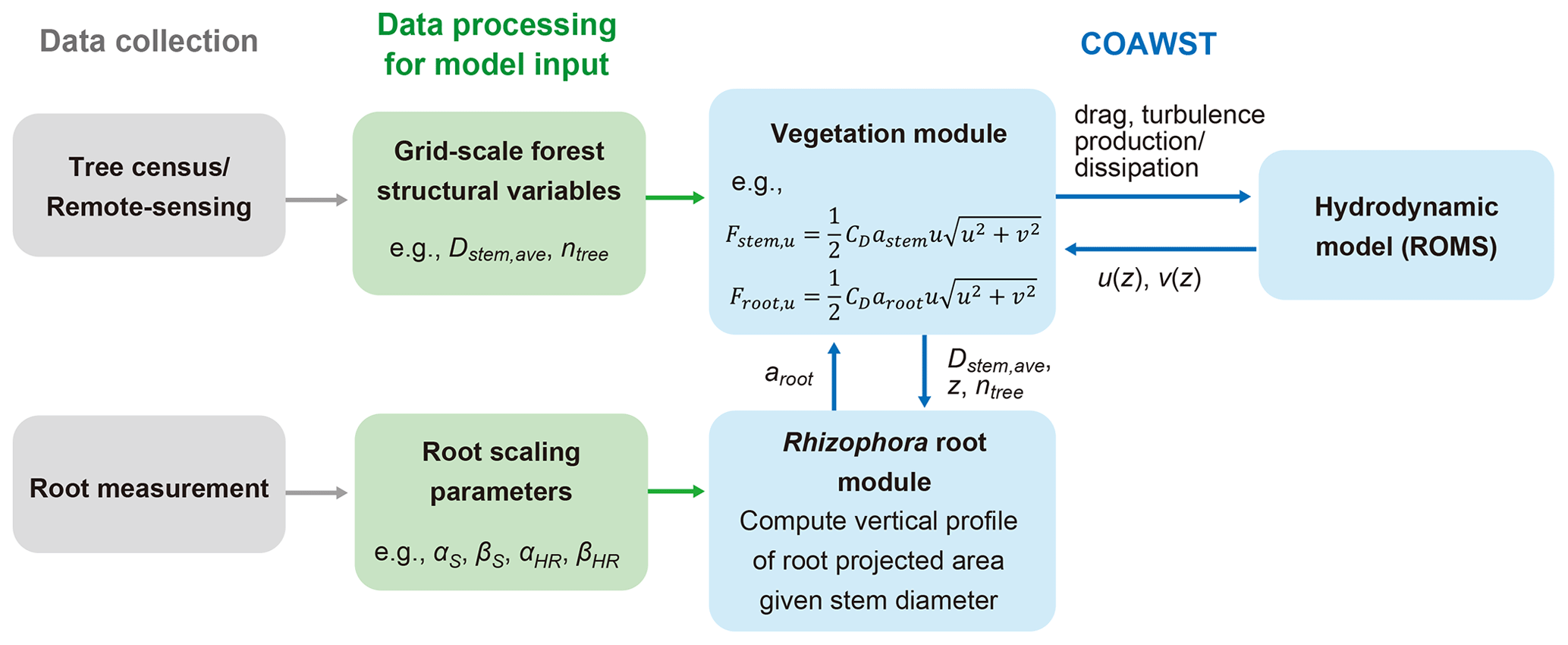
Figure 1 The proposed framework of modeling flow in Rhizophora mangrove forests using COAWST. D_stem,ave and n_tree are the respective mean stem diameter and tree density to be given in each grid; a_stem and a_root are the respective projected area density values for stem and root, where a_stem is a product of D_stem,ave and n_tree; and F_stem,u and F_root,u are the drag forces exerted on the u component of flow by the stem and root, respectively. See Sect. S3 and Table S1 for explanations of the root scaling parameters.

This paper considers velocities as temporally averaged unless otherwise specified. We did not consider the subgrid-scale spatial heterogeneity of velocity generated by vegetation, as in other modeling studies (e.g., King et al., 2012; Marsooli et al., 2016). The Reynolds number (Re) defined using the root diameter as the length scale could be higher than the value ensuring fully turbulent structures of root-generated wakes (Re>120; Shan et al., 2019), even for weak currents (∼ 1 cm s⁻¹), which could diminish the dependence of the drag coefficient (C_D) on Re. Thus, we treat C_D as a constant, as in Beudin et al. (2017). For simplicity, we present equations in a two-dimensional form on the x–z plane (zero velocity in the y direction), whereas the equations implemented in ROMS are three-dimensional (x–y–z), where x–y represents the horizontal plane and z represents the vertical direction.

2.1.1 Drag force

In Rhizophora mangrove forests, the stem and roots are the main components that exert drag in tidal flows. We partition the drag from Rhizophora mangroves (vegetation drag) into the contributions from stems and roots and calculated it using the quadratic drag law as follows:

$$\begin{array}{}\text{(1)}& \begin{array}{rl}{F}_{\mathrm{veg}}\left(z\right)& =F_{\mathrm{stem}}\left(z\right)+F_{\mathrm{root}}\left(z\right)={\displaystyle \frac{\mathrm{1}}{\mathrm{2}}}{C}_{\mathrm{D}}{n}_{\mathrm{tree}}{D}_{\mathrm{stem},\mathrm{ave}}u{\left(z\right)}^{\mathrm{2}}\\ & +{\displaystyle \frac{\mathrm{1}}{\mathrm{2}}}{C}_{\mathrm{D}}{a}_{\mathrm{root}}\left(z\right)u{\left(z\right)}^{\mathrm{2}},\end{array}\end{array}$$

where F_veg is the spatially averaged vegetation drag (m s⁻²); z is the height from the bed (m); F_stem and F_root are the contributions from stems and roots to F_veg, respectively; C_D is the drag coefficient; n_tree is the tree density (m⁻²); D_stem,ave is the mean stem diameter (m); a_root is the spatially averaged projected area density of roots (m⁻¹); and u is the flow velocity (m s⁻¹). We represented stems as cylindrical shapes with a vertically uniform diameter (Maza et al., 2017) and then calculated the F_stem using the cylinder drag model – the same equations introduced by Beudin et al. (2017) (Sect. S1 and Table 1). Here, we assumed a vertically constant and uniform drag coefficient (C_D) for stems and roots.

Table 1 Vegetation and hydrodynamic parameter settings for model testing against flume experiments (Exp 1 and Exp 2) in Maza et al. (2017) and field measurement in Yoshikai et al. (2022a). Figure S3 shows the location where the values of vegetation and hydrodynamic variables in the table were derived in Yoshikai et al. (2022a). Note that the values of vegetation and hydrodynamic variables in the flume in Maza et al. (2017) were converted to the real scale. The row for γ shows the values that best fit the measurements within the range of 0.8–1.6.

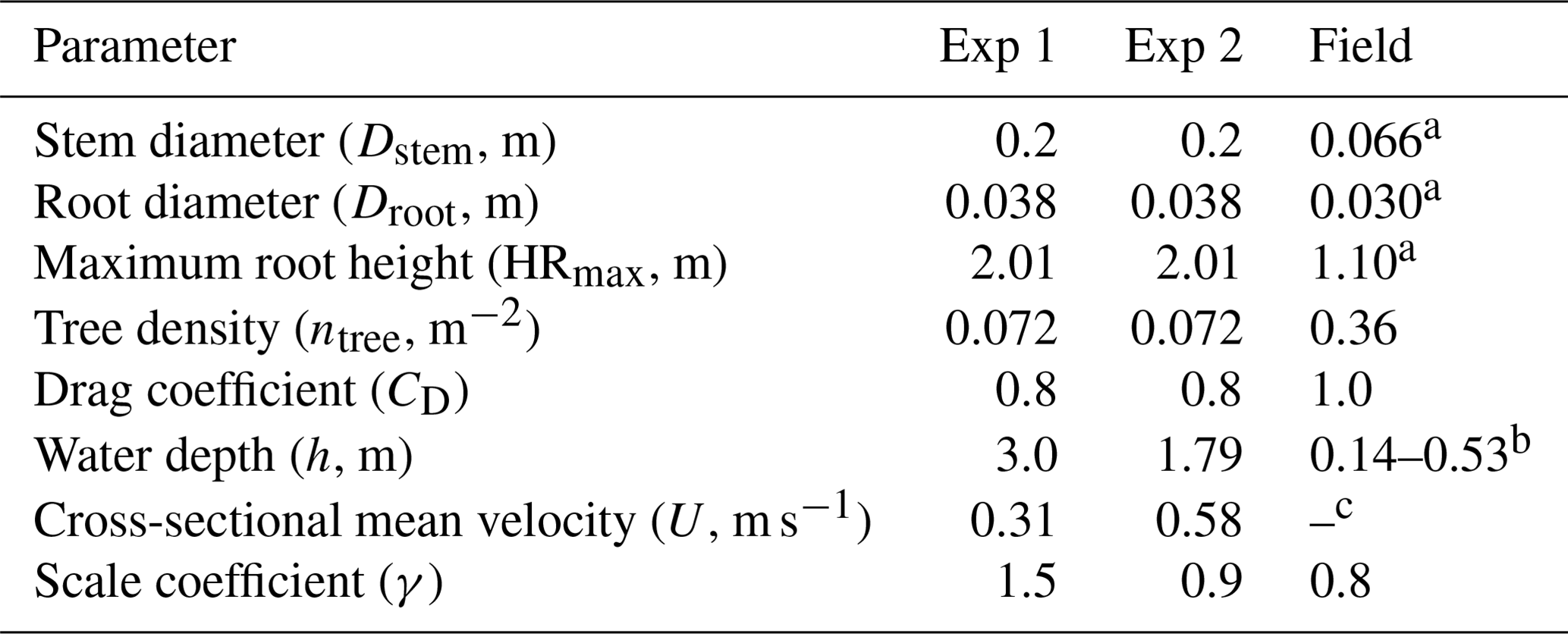
^a Mean value at the measurement site. ^b Water depth varies depending on the tidal phase (see Fig. 6a and e). ^c One of the target parameters for model prediction.

2.1.2 Turbulence

In ROMS, the generic length scale (GLS) model is implemented as the turbulence closure, where the equations can represent several two-equation closure models, such as the k–ε and k–ω models, by adjusting the model parameters (Umlauf and Burchard, 2003; Warner et al., 2005). In this paper, we present equations in the form of the k–ε model for reference purposes, as this is the most studied two-equation closure model for flows in vegetated areas (López and García, 2001; Katul et al., 2004; Defina and Bixio, 2005; King et al., 2012). Beudin et al. (2017) included an additional term for wake production due to vegetation (P_w) in the equation for turbulence kinetic energy (TKE) as follows:

$$\begin{array}{}\text{(2)}& {\displaystyle \frac{\partial k}{\partial t}}+u{\displaystyle \frac{\partial k}{\partial x}}={\displaystyle \frac{\partial }{\partial z}}\left({\displaystyle \frac{{\mathit{\upsilon }}_t}{{\mathit{\sigma }}_k}}{\displaystyle \frac{\partial k}{\partial z}}\right)+P_{\mathrm{s}}+B+P_{\mathrm{w}}-\mathit{\epsilon },\end{array}$$

where k is TKE (m² s⁻²); ν_t is the eddy viscosity (m² s⁻¹); σ_k is the turbulent Schmidt number for k (1.0); P_s, B, and P_w represent the production of k by shear, buoyancy, and wakes generated by vegetation (m² s⁻³), respectively; and ε is the turbulent dissipation (m² s⁻³). Similarly, they included an additional term (D_w) in the equation for ε as follows:

$$\begin{array}{}\text{(3)}& {\displaystyle \frac{\partial \mathit{\epsilon }}{\partial t}}+u{\displaystyle \frac{\partial \mathit{\epsilon }}{\partial x}}={\displaystyle \frac{\partial }{\partial z}}\left({\displaystyle \frac{{\mathit{\upsilon }}_t}{{\mathit{\sigma }}_{\mathit{\epsilon }}}}{\displaystyle \frac{\partial k}{\partial z}}\right)+{\displaystyle \frac{\mathit{\epsilon }}{k}}\left(c_{\mathrm{1}}{P}_{\mathrm{s}}+c_{\mathrm{3}}B-c_{\mathrm{2}}\mathit{\epsilon }\right)+D_{\mathrm{w}},\end{array}$$

where σ_ε is the turbulent Schmidt number for ε (1.3); c₁ (1.44), c₂ (1.92), and c₃ are the model constants, where the value of c₃ varies depending on the stratification state (Warner et al., 2005); and D_w is the dissipation rate of wakes (m² s⁻⁴). The wake production rate (P_w) is typically considered equal to the rate of work done by the flow against vegetation drag, i.e., P_w=F_vegu (Nepf, 2012). In contrast, the turbulence dissipation rate largely depends on the turbulence length scale in addition to the TKE, which requires a priori knowledge of the turbulence length scale of wakes to correctly predict D_w (King et al., 2012; Liu et al., 2017; Li and Busari, 2019).

Previous flume studies for flow through vegetated areas have shown that the stem diameter (or leaf width) is the plausible turbulence length scale of wakes (Tanino and Nepf, 2008; King et al., 2012). In the case of flow in Rhizophora mangrove forests, however, there are two potential length scales – the stem diameter and root diameter – that could significantly differ from each other (Maza et al., 2017). This variation makes it challenging to parameterize them into one representative length scale of wakes (L in Eq. S6 in Sect. S2). To resolve this, we partitioned the P_w and D_w into the terms for wakes generated by stems and roots, respectively, as follows:

$$\begin{array}{}\text{(4)}& {\displaystyle }{P}_{\mathrm{w}}=P_{\mathrm{w},\mathrm{stem}}+P_{\mathrm{w},\mathrm{root}}=F_{\mathrm{stem}}u+F_{\mathrm{root}}u,\text{(5)}& {\displaystyle }{D}_{\mathrm{w}}=D_{\mathrm{w},\mathrm{stem}}+D_{\mathrm{w},\mathrm{root}}=c_{\mathrm{2}}{\displaystyle \frac{P_{\mathrm{w},\mathrm{stem}}}{{\mathit{\tau }}_{\mathrm{stem}}}}+c_{\mathrm{2}}{\displaystyle \frac{P_{\mathrm{w},\mathrm{root}}}{{\mathit{\tau }}_{\mathrm{root}}}}.\end{array}$$

Here, P_w,stem and P_w,root (m² s⁻³) are the production of k by stem- and root-generated wakes, respectively; D_w,stem and D_w,root (m² s⁻⁴) are the dissipation rate of stem- and root-generated wakes, respectively; and τ_stem and τ_root (s) are the timescales of stem- and root-generated wakes, respectively. The latter variables are given by the following:

$$\begin{array}{}\text{(6a)}& {\displaystyle }{\mathit{\tau }}_{\mathrm{stem}}={\left({\displaystyle \frac{L_{\mathrm{stem}}^{\mathrm{2}}}{c_{\mathrm{w}}^{\mathrm{2}}{P}_{\mathrm{w},\mathrm{stem}}}}\right)}^{\mathrm{1}/\mathrm{3}},\text{(6b)}& {\displaystyle }{\mathit{\tau }}_{\mathrm{root}}={\left({\displaystyle \frac{L_{\mathrm{root}}^{\mathrm{2}}}{c_{\mathrm{w}}^{\mathrm{2}}{P}_{\mathrm{w},\mathrm{root}}}}\right)}^{\mathrm{1}/\mathrm{3}}.\end{array}$$

Here, L_stem and L_root (m) are the length scale of stem- and root-generated wakes, respectively, and c_w is the model constant. We set the mean stem diameter (D_stem,ave) and root diameter (D_root,ave) as L_stem and L_root, respectively.

We considered c_w in Eq. (6) as a calibration parameter, whereas Beudin et al. (2017) gave a value of 0.09. Tanino and Nepf (2008) predicted the TKE for a flow through an array of emergent cylinders with cylinder projected area density, a, and cylinder diameter, d, using $k=\mathit{\gamma }{\left(\frac{\mathrm{1}}{\mathrm{2}}{C}_{\mathrm{D}}ad\right)}^{\mathrm{2}/\mathrm{3}}{u}^{\mathrm{2}}$, where γ is the scale coefficient that needs to be empirically determined. We can relate c_w to γ as $c_{\mathrm{w}}={\mathit{\gamma }}^{-\mathrm{3}/\mathrm{2}}$ by applying the k–ε model to a limiting case of a steady, uniform, and neutrally stratified flow through homogeneous emergent vegetation such that all the terms in Eqs. (2) and (3) except for k, ε, P_w, and D_w can be neglected (King et al., 2012; Liu et al., 2017). We adjusted the value of c_w so that the corresponding γ value falls within a reported range (0.8–1.6; King et al., 2012; Xu and Nepf, 2020).

2.1.3 Root projected area density

We used the empirical Rhizophora root model (Rh-root model) developed by Yoshikai et al. (2021) as a predictor of the root projected area density (a_root) in Eq. (1). Based on allometric relationships characterized by some site- and species-specific root scaling parameters (α_S, β_S, α_HR, and β_HR in Eq. S7 in Sect. S3), the Rh-root model predicts the vertical profile of root projected area per vertical interval (dz; 0.05 m in this study) for a tree “i” (A_root,i(z) (m²)) from the stem diameter of the tree (D_stem,i), where the subscript “i” represents the tree index. In short, A_root,i(z) is expressed as $A_{\mathrm{root},i}\left(z\right)=f\left(D_{\mathrm{stem},i}\right)$, where f represents a function of the Rh-root model (see Sect. S3 for details).

The vertical profile of the spatially averaged projected area density of roots in each grid can be calculated as $a_{\mathrm{root}}\left(z\right)=n_{\mathrm{tree}}{\sum }_{i=\mathrm{1}}^{N_{\mathrm{tree}}}f\left(D_{\mathrm{stem},i}\right)/\left(N_{\mathrm{tree}}\mathrm{d}z\right)$, where n_tree is the tree density (m⁻²) and N_tree is the number of trees in each grid. While some variation in tree size (i.e., D_stem,i), and thereby f(D_stem,i), within a grid is expected, it would be convenient if the subgrid-scale variations could be parameterized using a grid-scale parameter for modeling purposes. In this study, we propose that the mean stem diameter (D_stem,ave) can be used for the parameterization as ${\sum }_{i=\mathrm{1}}^{N_{\mathrm{tree}}}f\left(D_{\mathrm{stem},i}\right)/N_{\mathrm{tree}}\approx f\left(D_{\mathrm{stem},\mathrm{ave}}\right)$, so that a_root≈ n_treef(D_stem,ave)/dz.

We investigated the above assumption using tree census data collected from three sites (Bak1, Bak2, and Fuk; see Fig. S1 and Sect. S4 in the Supplement for the map and description of the sites). Using the Rh-root model, we computed the vertical distribution of the mean projected area of individuals in the tree census plots, ${\sum }_{i=\mathrm{1}}^{N_{\mathrm{tree}}}f\left(D_{\mathrm{stem},i}\right)/N_{\mathrm{tree}}$, and its representation using the mean stem diameter, f(D_stem,ave), and compared them (Fig. 2). The results demonstrate that the use of D_stem,ave can represent the mean projected area density of individuals for all the three sites well, regardless of the differences in the forest structure (e.g., stem diameter distribution and tree density) and root scaling parameters (Table S1).

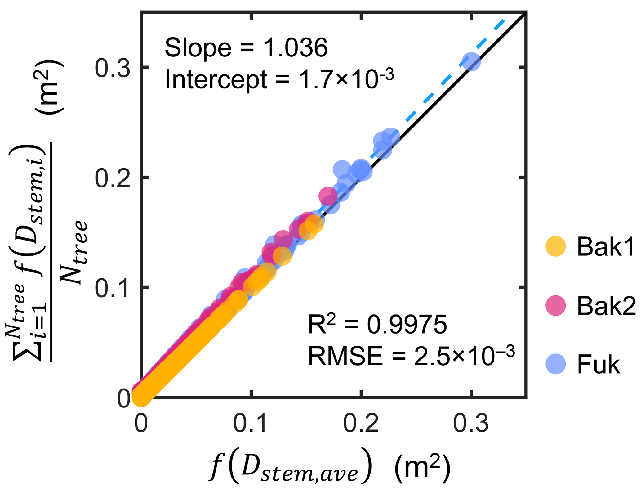
Figure 2 Comparison of the vertical profiles of the mean projected area per vertical height interval (dz; 0.05 m) of individuals in tree census plots from three sites (Bak1, Bak2, and Fuk), ${\sum }_{i=\mathrm{1}}^{N_{\mathrm{tree}}}f\left(D_{\mathrm{stem},i}\right)/N_{\mathrm{tree}}$, and its representation using the mean stem diameter, f(D_stem,ave), where N_tree is the number of Rhizophora trees in a plot, D_stem,ave is the mean stem diameter of Rhizophora trees in the plot, the subscript “i” represents the tree index, and f represents the function of the Rhizophora root model that gives the vertical profile of the projected root area of individuals. The black line indicates the 1:1 line and the dashed blue line indicates the best-fitting line.

2.2 Model testing

We tested the new model implemented in the COAWST framework against measurements of flow in a laboratory model of a Rhizophora mangrove forest by Maza et al. (2017) and in a planted Rhizophora mangrove forest in the field by Yoshikai et al. (2022a). Section S5 provides some descriptions of the implementation of the new model in COAWST. Both of the aforementioned studies provided detailed information on vegetation and hydrodynamic parameters that allow us to evaluate the model's performance. Specifically, the mangrove forests in both studies have a spatially uniform vegetation distribution due to the uniformly sized and evenly distributed trees (approximately in the case of the real mangrove forest in Yoshikai et al., 2022a). Moreover, both studies measured flow structures at a location where the flow is well developed, which eliminates the dependence of flow structures on the proximity to the forest's leading edge. Given these conditions, we tested the model using a model grid assuming a schematized mangrove forest with a uniform bed elevation and vegetation variables described below, not with a grid representing the actual geometric/topographic conditions of the flume/field. Table S3 summarizes the measured hydrodynamic variables in Maza et al. (2017) and Yoshikai et al. (2022a), the variables controlled in the model, and the target variables to be reproduced for each test case.

We created an orthogonal computational grid of 200 m × 200 m area with a 5 m horizontal resolution for the model runs (Fig. S2). We set 15 vertical layers with an approximately uniform layer thickness to be applied to the laboratory-based study of Maza et al. (2017). For the field-based study (Yoshikai et al., 2022a), the number of vertical layers was reduced to five because of the shallow water depths. To create a unidirectional flow in the model, we set the eastern and western boundaries of the model domain to closed (no water fluxes) and the northern and southern boundaries to open (Fig. S2). We then imposed water level differences between the northern and southern boundaries to drive the flow based on a pressure gradient, where the water fluxes through the boundaries are given to equate the local pressure gradient and the drag force (bed + vegetation). The model was run without wind in the simulation. When the flow steady state was attained in the simulation, we compared the flow condition at the center of the model domain with the measured values (Fig. S2). This means that the actual time series of the flow during the tidal cycle was not reproduced when the model was applied to the field mangrove forest; rather, steady states of flow were created for each flow measurement. Table 1 summarizes the key vegetation and hydrodynamic parameters for each test case.

We set different objectives for the model applications to laboratory- and field-based studies. The main objective of applying the model to a laboratory-based study is to examine the effectiveness of the formulations for the drag and turbulence terms (Eqs. 1–6), which were newly implemented in COAWST to predict the flow structures in the Rhizophora mangrove forest, compared with those predicted by the cylinder drag model. Here, we consider the vegetation frontal area density (a) as a known parameter. In contrast, the parameter a is usually unknown and needs to be predicted in the case of mangrove forests in the field. Hence, the main objective of the application to the field-based study is to examine the effectiveness of the proposed framework (Fig. 1) that includes the Rh-root model – the predictor of a – in COAWST, compared with the drag parameterizations proposed in previous studies. Table 2 summarizes the different model configurations tested to represent the impact of Rhizophora mangroves for applications to the laboratory- and field-based studies. Below, we describe an overview of the measurements by Maza et al. (2017) and Yoshikai et al. (2022a) and the model settings.

Table 2 Tested model configurations to represent the impact of Rhizophora mangroves against flume experiments (Exp 1 and Exp 2) in Maza et al. (2017) and field measurements in Yoshikai et al. (2022a). The parameters used in the table are as follows: n_tree – tree density; n_v – cylinder density; D_stem,ave – mean stem diameter; b_v – cylinder density; a_root – root projected area density; D_root,ave – mean root diameter; z₀ – bed roughness length; and N_layer – number of vertical layers of model grid.

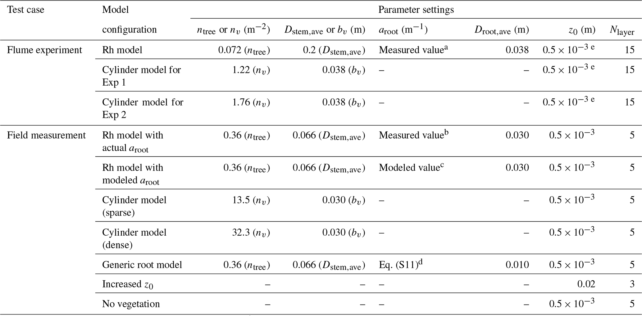
^a Corresponds to the value of black markers minus n_treeD_stem,ave in Fig. 3a. ^b Corresponds to the value of black markers minus n_treeD_stem,ave in Fig. 3b. ^c Corresponds to the value of blue markers minus n_treeD_stem,ave in Fig. 3b. ^d Corresponds to the value of light green markers minus n_treeD_stem,ave in Fig. 3b. ^e Assumed value.

2.2.1 Application to a laboratory-based study

The model Rhizophora mangrove forest created in the flume by Maza et al. (2017) was $\mathrm{1}/\mathrm{12}$ of the real scale, whereas we ran our model at the real scale, i.e., we converted the velocities in the flume to the real scale by keeping the Froude number (Table 1). The real-scale vertical profile of vegetation projected area density (a) is shown in Fig. 3a. Maza et al. (2017) fabricated the root systems based on the data in Ohira et al. (2013) and distributed the model trees in-line in the flume. Maza et al. (2017) created two flow conditions by varying the water depth (h) and cross-sectional mean velocity (U) (Exp 1 and Exp 2; Table 1) and measured the vertical profiles of velocities and TKE at five lateral positions in the model forest at which flows were fully developed (Table S3). We averaged the data taken at the five positions to estimate the spatial average of the velocity and TKE to be compared with the model output.

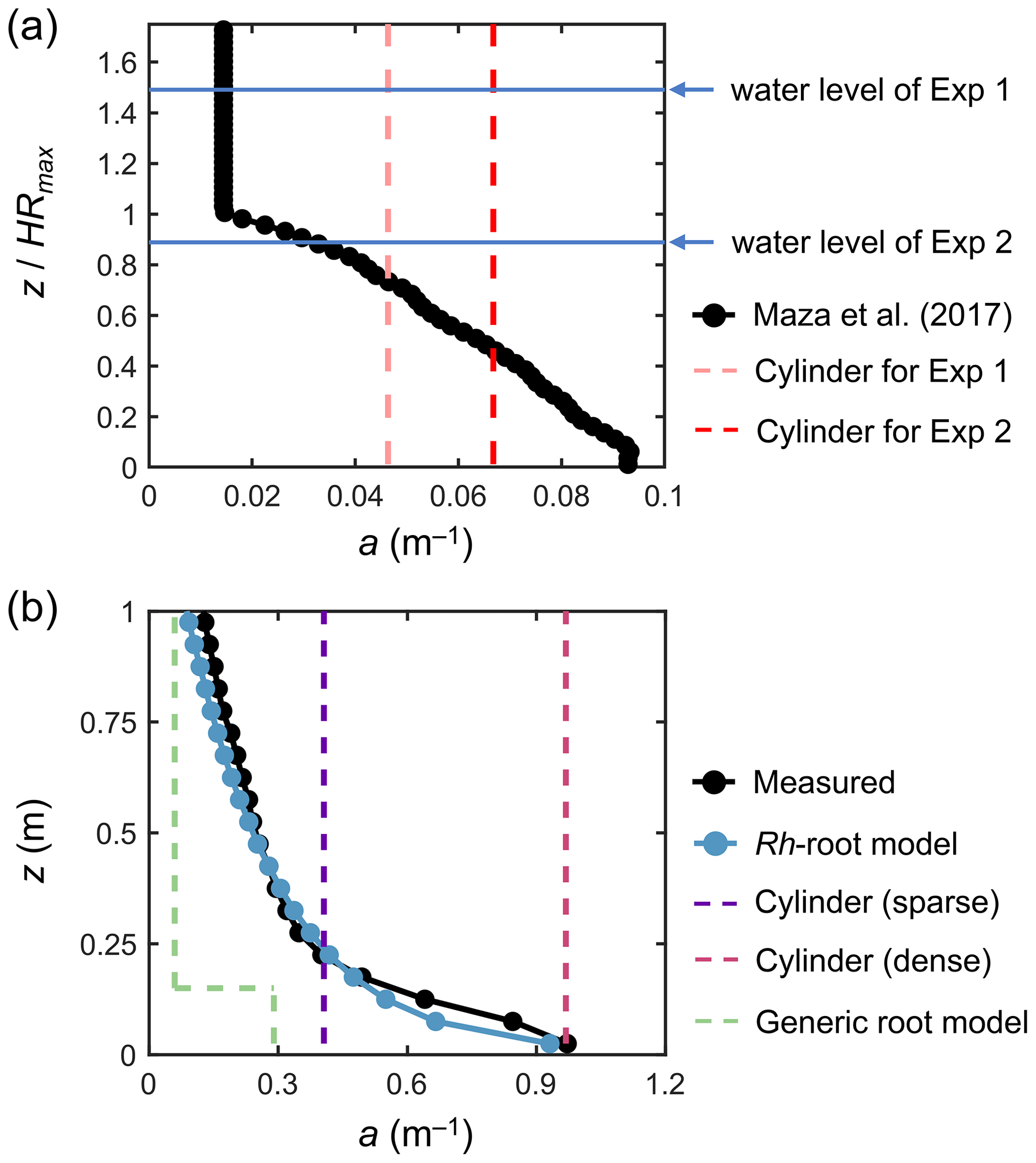
Figure 3 Vertical profiles of vegetation projected area density, a, in (a) a model Rhizophora mangrove forest examined by Maza et al. (2017) and (b) a real Rhizophora mangrove forest examined by Yoshikai et al. (2022a), where the values were calculated with dz = 0.05 m vertical interval (markers). HR_max is the maximum root height (2.01 m in Maza et al., 2017; Table 1). The modeled a using the Rh-root model in panel (b) is given by the Rhizophora root module using the parameters shown in Tables 1 and S1 (for Bak2). The projected area density of cylinder arrays (in panels a and b) and the a predicted using the generic mangrove root model (in panel b), which were used for comparison with the new model to represent the impacts of Rhizophora mangroves, are also shown (dashed lines).

We imposed the real-scale vertical profile of a examined in Maza et al. (2017) (black markers in Fig. 3a) over the model domain. This means that the Rh-root module that predicts a_root was not applied for the simulations performed here. We optimized the water levels at the boundaries to create the same flow conditions (h and U) at the center of the model domain as those in Exp 1 and Exp 2, respectively.

We used a value of 0.8 for the drag coefficient (C_D) in the model (Table 1), the value of which was derived in fully developed flows with high Reynolds numbers (>230) by Maza et al. (2017). The value of the bottom roughness (z₀) in the flume is unknown; hence, we set z₀ to 0.5 mm, which is the value derived in the field-based study (see Sect. 2.2.2). Due to the uncertainty in the bottom roughness, we did not include the modeled near-bed velocity and TKE for comparison with the measurements – velocity and TKE were insensitive to the bottom roughness. Another unknown parameter is the scale coefficient in the turbulence closure, γ ($=c_{\mathrm{w}}^{\mathrm{2}/\mathrm{3}}$; see Sect. 2.1.2). We ran the model by varying γ in a reported range (0.8–1.6) with an interval of 0.1 to seek a value that produced the best fit with the measurements, mostly for the TKE profile. Figure S4 provides the model sensitivity to varying γ for the prediction of TKE profiles.

In addition to the simulation using the actual a (black markers in Fig. 3a), referred to as the “Rh model”, we tested the use of the cylinder drag model, referred to as the “cylinder model” (Table 2). We defined the cylinder array for Exp 1 and Exp 2, respectively, where the cylinder projected area density was set equal to the depth average of the actual a for each case (dashed lines in Fig. 3a); we set the cylinder diameter equal to the root diameter of the model Rhizophora trees (0.038 m; Table 1). The cylinder height was set much higher than the water level to create a condition under which cylinders spanned the entire water column – this also applies to the cylinder drag model examined in the next section.

2.2.2 Application to a field-based study

Yoshikai et al. (2022a) measured vegetation and hydrodynamic parameters at 17-year-old planted stands of Rhizophora apiculata in a mangrove forest locally known as Bakhawan Ecopark in Aklan, Philippines (Fig. S3). The site corresponds to Bak2 in Fig. 2. Like in the flume condition of Maza et al. (2017), approximately uniformly sized trees are evenly distributed. The measured spatially averaged vegetation projected area density (a) at the site is shown in Fig. 3b. Due to the higher complexity of the root systems and higher tree density (Table 1), the a near the bed showed almost a 10-fold higher value than that in Maza et al. (2017) (Fig. 3). Yoshikai et al. (2022a) conducted hydrodynamic measurements during ebb tides on 10 and 11 September 2018 that corresponded to spring tide conditions. The measured parameters were the water depth, the spatially averaged velocity profile (based on measurements at four locations), the water surface slope along a major flow direction, and the bed shear stress (Table S3). The flow at the site is considered to be fully developed.

We imposed the measured water surface slope at the boundaries to drive the flow: the water depths at the boundaries were adjusted to realize the same water depth at the center of the model domain as the measurement. We used a value of 1.0 for the drag coefficient (C_D) and 0.5 mm for the bottom roughness (z₀) based on the results in Yoshikai et al. (2022a) (Table 1). As in the previous section, we changed the value of γ in a reported range (0.8–1.6) with an interval of 0.1 to seek a value that produced the best fit with the measured velocity profile. Note that the TKE profile has not been measured in the field; thus, it could not be validated.

We tested seven different model configurations (Table 2): the Rh model using the measured values for a_root (actual a; black markers in Fig. 3b), the Rh model using the modeled a_root (blue markers in Fig. 3b), the cylinder model using two different cylinder densities (sparse and dense; dashed purple and red lines in Fig. 3b), use of the other predictive model for Rhizophora root structures used in Xie et al. (2020) as the predictor of a_root in Eq. (1) (termed “generic root model”; dashed green line in Fig. 3b), increased bed roughness (z₀), and a case without imposing the vegetation drag (“no vegetation”). Among these, the proposed framework (Fig. 1) was employed for the Rh model case using the modeled a_root (the Rhizophora root module provided the a_root in the simulation) with input parameters of measured mean stem diameter (D_stem,ave) and tree density (n_tree). We set the sparse cylinder case based on Horstman et al. (2013), who suggested the use of vegetation geometry measured at a height of around 0.25 m for cylinder array approximation. We set the dense cylinder array to produce an equivalent resistance to Manning's coefficient of 0.14 at a water depth of 0.5 m, a value often used to represent the drag from mangroves (e.g., Zhang et al., 2012; Menéndez et al., 2020). The generic root model used in Xie et al. (2020) predicts the mangrove root structure (a_root) as an array of vertical cylinders with a fixed diameter (D_root) and height (H_root) from a given stem diameter and tree density (see Text S6 for the model details). We use the term “generic” because Xie et al. (2020) used this model to represent root structures of several different mangrove genera, including Rhizophora. Here, we used the same parameter values for D_root and H_root as those used in Xie et al. (2020) for Rhizophora root structures: D_root=0.01 m and H_root=0.15 m. The vegetation frontal area (stem + root) predicted by the generic root model using measured mean stem diameter ($D_{\mathrm{stem},\mathrm{ave}}=\mathrm{0.066}$ m) and tree density (n_tree=0.36 m⁻²) is shown in Fig. 3b. Here, the predicted a_root is used for calculating the drag from roots in Eq. (1). In addition, $D_{\mathrm{stem},\mathrm{ave}}=\mathrm{0.066}$ m and D_root=0.01 m were applied for L_stem and L_root in the turbulence dissipation term of Eq. (6) (Table 2). For the case of increased z₀, we reduced the number of vertical layers from five to three and set z₀=0.02 m (Table 2; see Sect. S7 for details on the bed shear stress calculation and the choice of the value). We note that the z₀ value equivalent to Manning's coefficient of 0.14 at 0.5 m water depth is z₀=0.22 m, but we were able to increase the value up to 0.02 m due to the numerical limitation of the logarithmic velocity profile assumption implemented in COAWST (Eq. S13). For the case without vegetation, z₀ is kept as 0.5 × 10⁻³ m, the same as the other vegetated cases. In the increased z₀ and the no vegetation cases, the bed shear stress is the main force to equate with the imposed pressure gradient.

3 Results

3.1 Comparison with a laboratory-based study

Figure 4 shows a comparison of the modeled and measured vertical profiles of velocity (u) and TKE (k) normalized by cross-sectional mean velocity (U) for Exp 1 and Exp 2, the conditions examined by Maza et al. (2017). The profile of normalized velocity was reasonably predicted by the Rh model (Fig. 4a, c), especially in the lower part of the root system (i.e., $z/{\mathrm{HR}}_{\max }\mathit{<}\mathrm{0.6}$) in Exp 1 where the velocity was greatly attenuated compared with the upper part or above the root system (Fig. 4a). The higher values of γ led to more homogeneous velocity profiles because of the enhanced vertical momentum exchange by the elevated TKE, while the sensitivity to varying γ was not significant. The Rh model also predicted the overall trend in the normalized TKE profile measured by Maza et al. (2017) well for both Exp 1 and Exp 2 by adjusting the value of γ (Fig. 4b, d). Notably, the Rh model captured the distinct vertical variations in TKE observed in Exp 1 when γ=1.5 (Fig. 4b) well, while the best fit was obtained when γ=0.9 (Fig. 4d) for Exp 2. Overall, γ = 1.2 produced the smallest total error in Exp 1 and Exp 2 between the model and measured values (Fig. S4). It under- and overestimated the TKE averaged over the measurement section by about 20 % and 40 % for Exp 1 and Exp 2, respectively (Fig. 4b, d), which is generally fairly good agreement for predicting TKE.

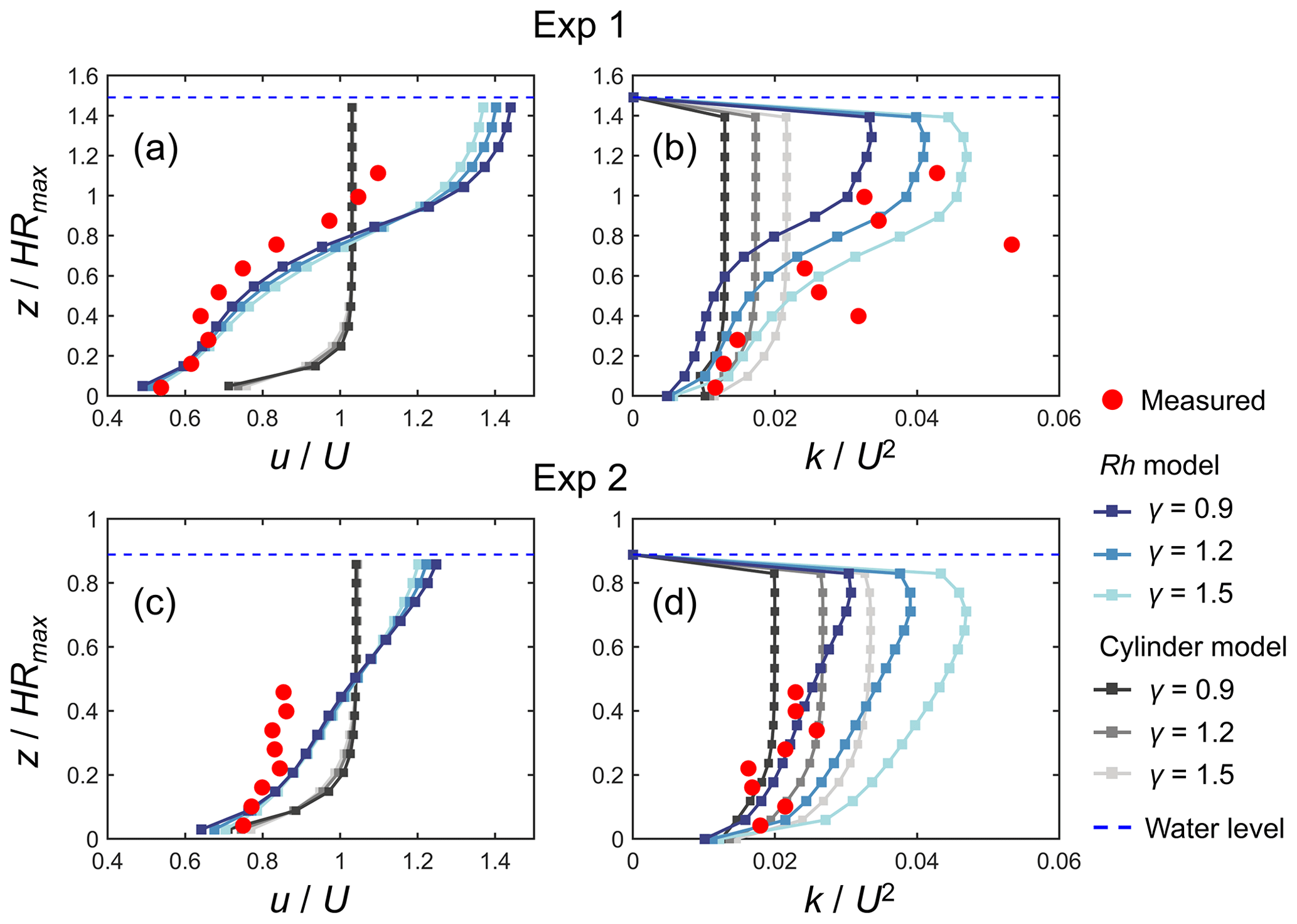
Figure 4 Comparison of the vertical profiles of (temporally and spatially averaged) velocity (u) and turbulent kinetic energy (k) normalized by the cross-sectional mean velocity (U) predicted by COAWST with different model configurations (Rh model and cylinder model) using different γ values and measurements by Maza et al. (2017) for (a, b) Exp 1 and (c, d) Exp 2. HR_max is the maximum root height. Data on the measured values are provided in Table S4.

In contrast to the Rh model, the cylinder model predicted the nearly uniform vertical profile of velocity except for the region close to the bed for both Exp 1 and Exp 2 and largely deviated from the measurements (Fig. 4a, c). The TKE predicted by the cylinder model also showed a nearly uniform vertical profile (Fig. 4b, d). While the cylinder model showed comparable TKE to the Rh model in the lower part of the root system (i.e., $z/{\mathrm{HR}}_{\max }\mathit{<}\mathrm{0.4}$) for both cases, it showed a significantly smaller TKE in the upper region compared with the Rh model and the measurements.

3.2 Comparison with a field-based study

Figure 5 shows the comparison of modeled velocity profiles with measurements by Yoshikai et al. (2022a) for some selected tidal phases in a Rhizophora mangrove forest (Bakhawan Ecopark). The Rh model using the measured profile of root projected area density (actual a_root) predicted the overall trend in measured velocity profiles in various tidal phases well (Fig. 5a). However, the model seemed to have underestimated the velocity attenuation from the surface to the bottom, which resulted in slightly higher near-bottom velocity and/or lower near-surface velocity compared with the measurements. Here, the value of γ was chosen as 0.8 from the range of 0.8–1.6 (Table 2), which produced the best fit with the measured velocity profile. The Rh model using the modeled a_root provided by the Rhizophora root module showed comparable performance with the use of actual a_root with respect to predicting the velocity profile (Fig. 5a). However, although not significant, the use of modeled a_root tended to further underestimate the velocity attenuation from the surface to the bottom due to the underestimation of a_root near the bed by the Rh-root model (Fig. 3b).

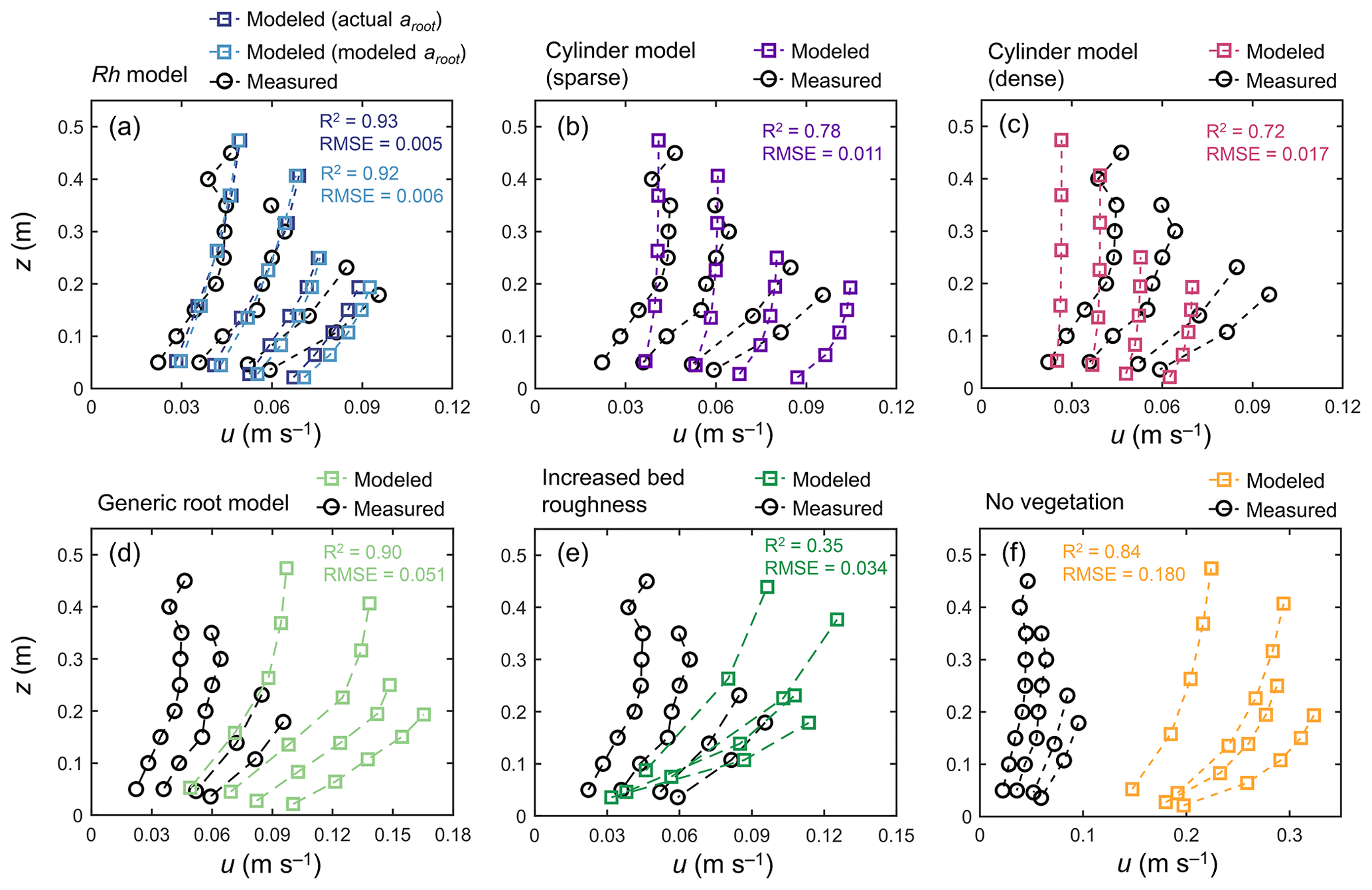
Figure 5 Comparison of the vertical profiles of velocity (u) predicted by COAWST employing (a) the Rh model using an actual and modeled root projected area density profile (a_root), (b) the cylinder model with a sparse and (c) dense array, (d) the generic root model, (e) increased bed roughness as an approximation of vegetation drag, and (f) without imposing vegetation drag (no vegetation), and measurements by Yoshikai et al. (2022a) for some selected tidal phases during the measurement period. The root-mean-square error (RMSE) and R² values of the modeled u against the measured data are also shown, for which computation of the predicted value at the height of the measurement point was obtained by the interpolation of u computed at adjacent vertical layers. Data on the measured values are provided in Table S5.

The cylinder model with sparse arrays showed comparable velocities to measurements near the water surface but significantly overestimated the velocities near the bed (Fig. 5b). Alternatively, the dense arrays showed comparable velocities near the bed but significantly underestimated the velocities near the water surface (Fig. 5c). The use of the generic root model as a predictor of a_root in Eq. (1) led to significant overestimation of velocities over the depths (Fig. 5d) due to the significantly underestimated vegetation projected area density (Fig. 3b). The approximation of mangrove drag in z₀ (increased bed roughness case) predicted the significant attenuation of flow velocity from the surface to the bottom due to the large bottom friction, which did not represent the actual conditions of the velocity profile in the Rhizophora mangrove forest well (Fig. 5e). The condition involving not imposing vegetation drag effects led to a large overestimation of the velocities, approximately 3–4 times larger than the measurements (Fig. 5f).

A fairly good reproduction of tidal flows by the Rh model can also be seen in the agreement with the measurements for the time series of channel-mean velocity (U), (spatially averaged) velocity at z=0.05 m (u_bottom), and bed shear stress (τ_bed) during the 2 d measurement period (Fig. 6). Note that we estimated the model prediction of velocity at z=0.05 m from linear interpolation of velocities computed at adjacent vertical layers. The u_bottom was generally overestimated by about 15 % (Fig. 6c, g), as also seen in Fig. 5a. As a result, the τ_bed was overestimated by about 30 % by the model, which is still a reasonable agreement (Fig. 6d, h). As demonstrated in Fig. 5a, the Rh model employing the modeled a_root also showed a comparable performance for the time series data (Fig. 6).

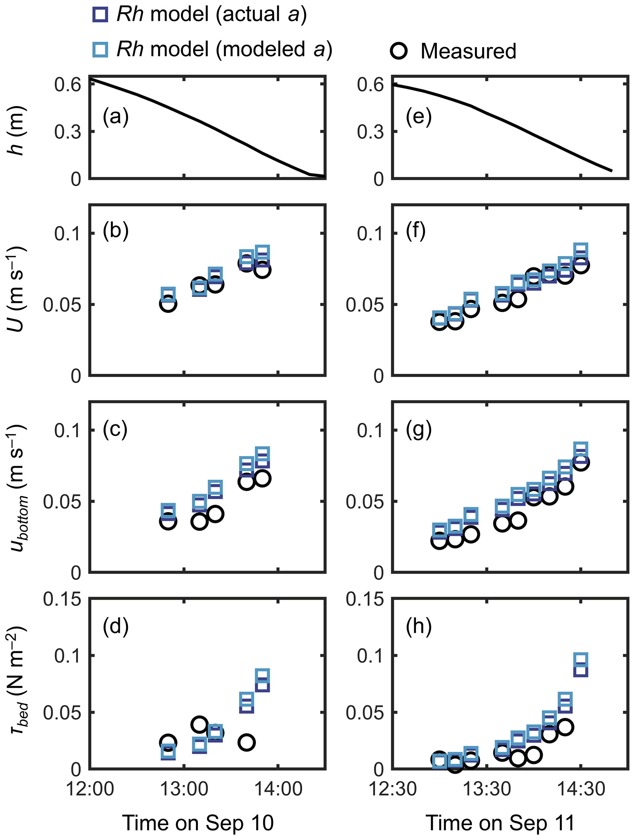
Figure 6 Time series of (a, e) measured water depth (h), measured and predicted (b, f) cross-sectional mean velocity (U), (c, g) (spatially averaged) velocity at z=0.05 m, and (d, h) bed shear stress (τ_bed) during the 2 d measurement period in Bakhawan Ecopark. The measured values are from Yoshikai et al. (2022a). The predicted values are obtained via COAWST by employing the Rh model using an actual and modeled root projected area density profile (a_root). Data on the measured values are provided in Table S6.

The cylinder model with a sparse array led to a significant overestimation trend for U, u_bottom, and τ_bed over the tidal phases, especially when the water depth decreased (Fig. 7). The cylinder model with a dense array led to the underestimation of U in most of the tidal phases but showed an agreement with the measurements for u_bottom and τ_bed (Fig. 7). The use of a generic root model resulted in consistently higher U, u_bottom, and τ_bed compared with the measured values (Fig. 8), similar to the trend seen in Fig. 5d. Although the case using increased z₀ showed a large overestimation of flow velocities, as much as the case using the generic root model when the water depth is relatively high (e.g., h>0.3 m), it approached the measured values with decreasing water depth (Fig. 8); we will discuss these contrasting results in the following section. Because the bed drag is the main force to counteract the imposed pressure gradient in the increased z₀ case, the τ_bed showed a large overestimation over the tidal phases, as expected (Fig. 8c, f). The model without imposing vegetation drag led to a large overestimation of these parameters over the tidal phases (Fig. S5), similar to the result shown in Fig. 5f.

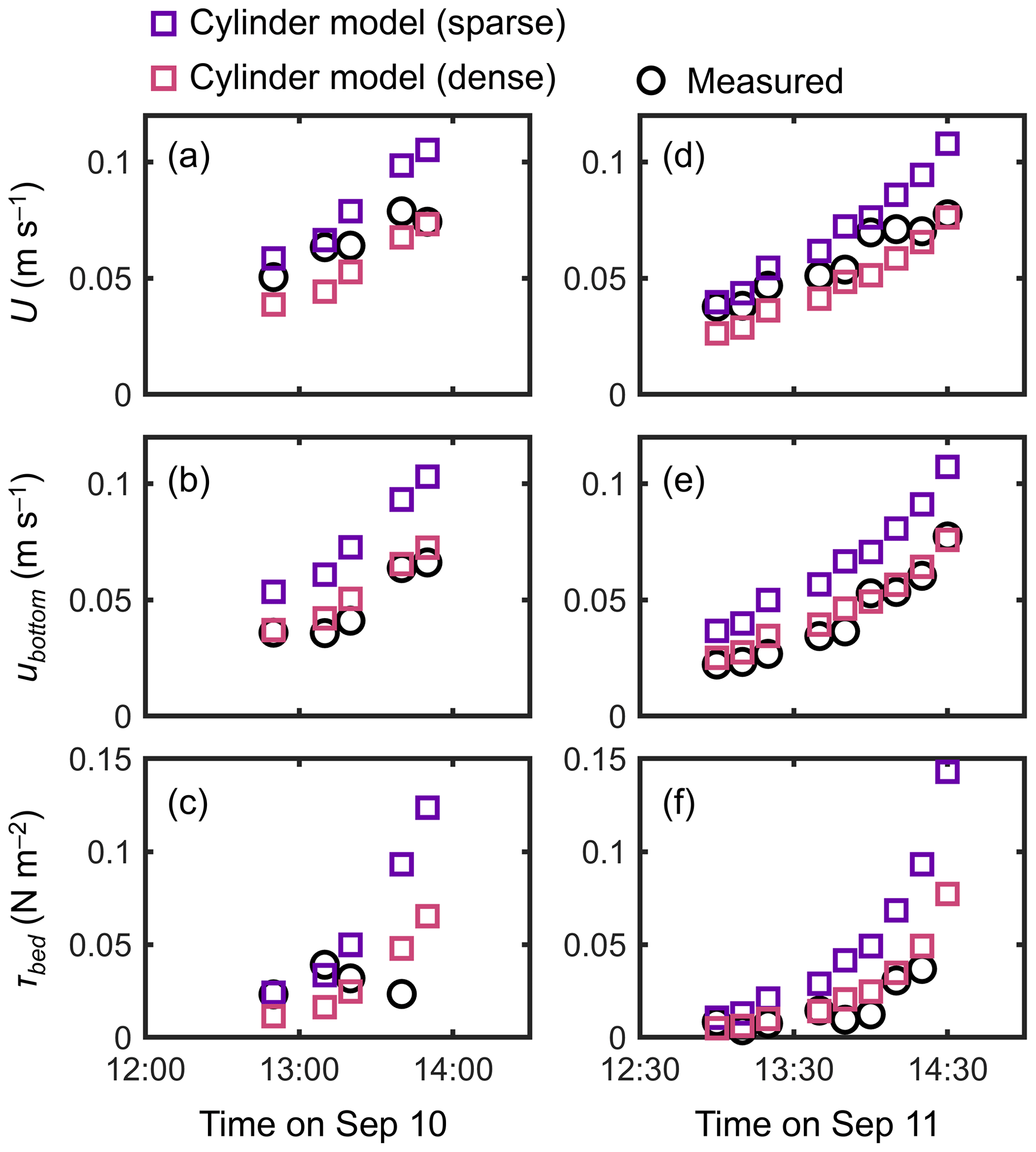
Figure 7 Time series of measured and predicted (a, d) cross-sectional mean velocity (U), (b, e) (spatially averaged) velocity at z=0.05 m, and (c, f) bed shear stress (τ_bed) during the 2 d measurement period in Bakhawan Ecopark. The measured values are from Yoshikai et al. (2022a). The predicted values are obtained via COAWST by employing the cylinder model with sparse and dense arrays.

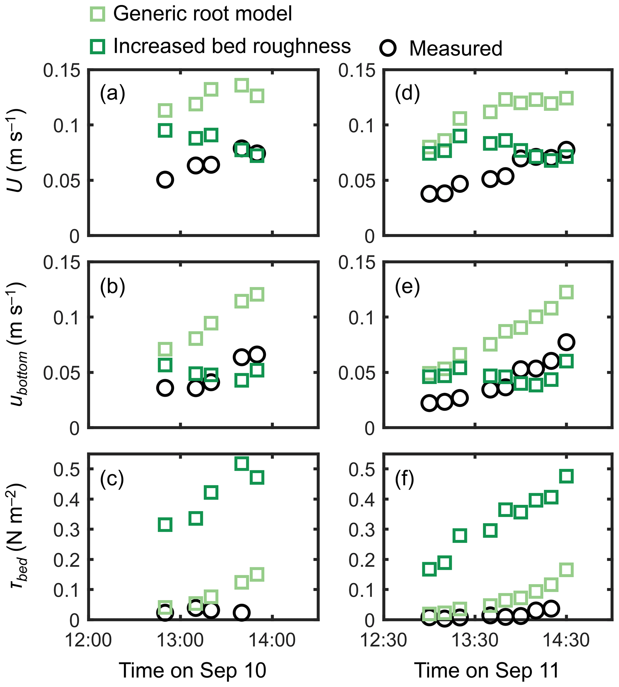
Figure 8 Time series of measured and predicted (a, d) cross-sectional mean velocity (U), (b, e) (spatially averaged) velocity at z=0.05 m, and (c, f) bed shear stress (τ_bed) during the 2 d measurement period in Bakhawan Ecopark. The measured values are from Yoshikai et al. (2022a). The predicted values are obtained via COAWST by employing the generic root model and the increased bed roughness as an approximation of drag due to mangroves, respectively.

4 Discussion

4.1 Performance of the previously proposed drag parameterization

Due to the general lack of information on the vertically varying projected area of complicated root systems, the drag due to Rhizophora mangroves has been represented by increased Manning's roughness coefficient values (e.g., Zhang et al., 2012) or an array of cylinders with an arbitrary cylinder density (Horstman et al., 2013; Xie et al., 2020) in hydrodynamic models with a two-dimensional configuration. We evaluated these drag parameterizations using the cylinder array or increased bed roughness approximation in a three-dimensional configuration (dashed lines in Fig. 3 for the cylinder arrays). Consistent with previous studies (Liu et al., 2008; King et al., 2012), the cylinder array approximations showed the vertically uniform velocity and TKE profile except near the bed, which largely deviated from the measurements (Figs. 4, 5). Moreover, for the tidal flows with changing water depth, the two different cylinder array configurations (sparse and dense) failed to capture the velocity changes over the tidal phases (Fig. 7) due to their inability to capture the changes in the submerged vegetation projected area of Rhizophora mangroves.

The generic mangrove root model used in Xie et al. (2020) predicts the Rhizophora root system as an array of vertical cylinders with a fixed height and diameter. However, the root system structures of Rhizophora mangroves cannot be simply approximated as an array of vertical cylinders, as shown in Fig. 3b. Although the shape of the vertical profile of velocity predicted using the generic root model resembles that of observed profiles, as indicated by the high R² value in Fig. 5d, the model failed to predict the absolute values, as indicated by the high RMSE, due to the significant underestimation of a (Fig. 3b). Because the shape of a predicted by the generic root model is similar to that of submerged vegetation, it is expected that the velocity inflection at the top of the root zone (z=H_root) will form as the projected area density of roots (a_root) further increases (e.g., King et al., 2012; Nepf, 2012), which will cause the results to deviate further from the actual velocity profiles.

Unlike the cylinder array approximations including the generic root model where the total projected area of submerged cylinders changes with the water depth, the approximation with increased bed roughness inherently assumes an invariant area of obstructions to flows. This means that the impact of bed roughness on flow velocity becomes more significant as the water depth decreases. This effect can be seen in the prediction of cross-mean flow velocity (U) at different tidal phases where the predicted U, which was largely overestimated under a relatively high water depth (h>0.3 m), approached the measured values as the water depth decreased, unlike the case using the generic root model (Fig. 8b, e). The approximation with increased bed roughness led to the large overestimation of τ_bed (Fig. 8c, f), thereby making it unsuitable for applications to sediment transport modeling in mangrove forests. Overall, none of the previously proposed drag parameterization sufficiently captured the flow structures in the Rhizophora mangrove forests examined in this study.

4.2 Performance of the new model

We proposed a new drag and turbulence model for flows in Rhizophora mangrove forests that works in the three-dimensional hydrodynamic model (ROMS) implemented in the COAWST framework. The model explicitly accounts for the vertically varying projected area of the root systems for drag force and TKE production in a three-dimensional configuration. In addition, the model accounts for the two different length scales of wakes (root- and stem-generated wakes) in the turbulence closure model (the k–ε model in this study), which is an aspect that none of the modeling studies have examined yet (e.g., López and García, 2001; King et al., 2012). With the relatively simple modifications made to the equations introduced by Beudin et al. (2017) (Eqs. 1, 4, 5, 6), our results showed significantly improved reproducibility of ROMS for the vertical profiles of velocity and TKE as well as velocity changes over the tidal phases in Rhizophora mangrove forests (Figs. 4, 5, 6). The new model also reasonably predicted the bed shear stress along with these parameters (Fig. 6d, h). Although some studies have accounted for the vertically varying vegetation projected area in hydrodynamic models for salt marshes (Temmerman et al., 2005) or mangrove forests with Rhizophora stands (Horstman et al., 2013, 2015), the efficacy of accounting for the vegetation three-dimensional structures in the model has not been demonstrated. Overall, this is the first modeling study to introduce a realistic representation of the influences of Rhizophora mangrove morphological structures on the flow that has been validated with existing data. The good performance of the model in both the modeled and real Rhizophora mangrove forests suggests the model's applicability to forests with a vegetation density a in the range of 0.09–0.9 m⁻¹ near the bed (Fig. 3) and an in-line tree distribution like planted mangrove forests. However, the model's applicability to forests with a>0.9 m⁻¹ and/or heterogeneous tree sizes and distributions, a condition often observed in natural mangrove forests, needs further investigation in future studies.

The laboratory-based study of Maza et al. (2017) provided valuable data for evaluating the new model for TKE in a Rhizophora mangrove forest, which are currently unavailable from field-based studies. They observed elevated TKE in the upper root zone and above the root zone ($z/{\mathrm{HR}}_{\max }\mathit{>}\mathrm{0.5}$; Fig. 4b). Maza et al. (2017) discussed TKE production by shear (P_s in Eq. 2) as one of the main reasons for the elevated TKE. However, we found that the different dominance of the root- and stem-generated wakes over the depth can explain these observations. For instance, the lower root zone that is dominated by root-generated wakes with a length scale set as the root diameter (0.038 m; Table 2) resulted in a higher dissipation rate (Eq. 6a), and thus lower TKE (Fig. 4b). On the other hand, the higher root zone dominated by stem-generated wakes with the length scale set as the stem diameter (0.2 m; Table 2) resulted in a lower dissipation rate (Eq. 6b), and thus higher TKE (Fig. 4b). This result is similar to the observation by Xu and Nepf (2020), who found a vertically varying turbulence integral length scale in a canopy of salt marsh plants of the genus Typha. Without accounting for the two different length scales, the model failed to reproduce the TKE profile while the velocity profile remained similar, suggesting the minor importance of shear production in reproducing the TKE (Fig. S6). The model also predicted the gradually increasing TKE upwards in the lower root zone ($z/{\mathrm{HR}}_{\max }\mathit{<}\mathrm{0.5}$), which is consistent with the measurements (Fig. 4b, d). While the model showed good reproducibility of the TKE profile, it should be noted that different γ values produced the best fit with the measurements for Exp 1 and Exp 2 (Fig. 4b, d). At this moment, the exact explanation for this observation is yet to be determined: whether it can be attributed to measurement uncertainty or processes that were not represented in the model. Further research on the turbulence structures in Rhizophora mangrove forests is needed. Unlike the TKE profiles predicted for the model mangrove forest, the TKE predicted for the field mangrove forest (Bakhawan Ecopark) that has a much higher vegetation complexity (higher a; Fig. 3) showed nearly uniform vertical profiles (Fig. S7); these results cannot be validated at this moment due to the lack of necessary data. Field studies on turbulence structures are likewise needed in this sense.

From the results shown, we highlight the importance of accounting for the vertically varying projected area of the root systems with a three-dimensional configuration for capturing the flow structures (Figs. 4–8). The model predictability is therefore dependent on the root projected area, which is typically unknown and labor-intensive to measure (Yoshikai et al., 2021). For practical use of the model, we implemented an empirical model for the Rhizophora root system (Rh-root model; Fig. 1) in COAWST with parameterization of subgrid-scale tree variations (Fig. 2) that enables model application without rigorous measurements of root structures. The simulation for flows in Bakhawan Ecopark using the modeled a_root provided by the Rhizophora root module showed almost identical results to that using the measured a_root in the field (Figs. 5, 6). This indicates the applicability of the model framework for predicting the flows in real Rhizophora mangrove forests. The grid-scale parameters required are mean stem diameter (D_stem,ave) and tree density (n_tree), which are included in basic information collected during tree census surveys (Simard et al., 2019; Suwa et al., 2021). Although the process of collecting these spatial data exceeds the scope of the study, we expect that even remotely sensed data such as airborne lidar (Jucker et al., 2017; Dai et al., 2018) or UAV optical imagery (Otero et al., 2018), which can detect basic tree features (e.g., tree height and crown width) that have a strong relationship with stem diameter (Jucker et al., 2017; Azman et al., 2021), can provide such information effectively. Obtaining the root scaling parameters requires field surveys (Fig. 1); however, these parameters can be relatively easily obtained by sampling 10–20 trees at the site (see Yoshikai et al., 2021, 2022a, for the procedure). The collection of these data is far less exhaustive than extensively measuring the vertical profile of a_root in the area of interest, as done by Horstman et al. (2015). Therefore, the model presented in this study may achieve a realistic forest-scale numerical modeling of flows in Rhizophora mangrove forests in the field.

4.3 Further model improvement

In order to extend the application of the presented model to sediment transport modeling, an accurate representation of vegetation impacts on both mean flow and turbulence structures that control sediment horizontal flux, retention/erosion, and turbulent mixing, is of primary importance (Nardin and Edmonds, 2014; Xu et al., 2022). Specifically, the greatly reduced near-bed velocity compared with the upper region that may significantly contribute to the sediment retention function of Rhizophora mangroves may be a key factor for sediment transport modeling in this kind of forest, which was captured by the new model only (Rh-model in Figs. 4 and 5). While we expect the improved prediction of the sediment transport process in Rhizophora mangrove forests given the improved prediction of overall flow structures using the presented new model, future studies on model application and validation with the field data on sedimentary processes are needed.

Several recent laboratory-based studies have shown that the turbulence generated by vegetation could contribute to sediment erosion; in that case, TKE may be a better predictor of erosion rate than bed shear stress (Tinoco and Coco, 2016; Yang and Nepf, 2018; Liu et al., 2021). Currently, most numerical models evaluate sediment erosion based on bed shear stress, even for the regions with vegetation (e.g., Zhu et al., 2021; Breda et al., 2021; Zhang et al., 2022). Accounting for the impact of vegetation-generated turbulence on sediment erosion in the model may be the next step to better represent the sediment transport process in Rhizophora mangrove forests, where the presented model has the potential to contribute to the consideration of the aforementioned impact. However, insights into the effects of turbulence on sediment erosion in Rhizophora mangrove forests are very limited at present, necessitating further laboratory- and field-based studies.

In order to predict the long-term geomorphic evolution of mangrove forests, the interactive feedback of vegetation–flow–sediment needs to be precisely simulated (van Maanen et al., 2015; Rodríguez et al., 2017; Xie et al., 2020). This process involves dynamic vegetation models that can capture long-term changes in root structure complexity in accordance with forest growth/development (e.g., Xie et al., 2020) – a process poorly represented in previous studies for Rhizophora mangrove forests. An advantage of the proposed model is that the root structures of Rhizophora mangroves are allometrically predicted in the hydrodynamic model from the basic forest structural variables – mean stem diameter and tree density, of which long-term dynamics can now be predicted using dynamic vegetation models for mangroves (e.g., Yoshikai et al., 2022b). The coupling of the hydrodynamic–sediment transport model and the dynamic vegetation model is one of the next challenges that will advance our understanding of the long-term geomorphic evolution in mangrove forests.

5 Concluding remarks

Modeling flow in Rhizophora mangroves is challenging due to their complex root structures. This paper presents a new model to represent the impacts of Rhizophora mangroves on flow that is implemented in the COAWST model framework with the aim of establishing a better understanding of hydrodynamics in mangrove forests. The new model explicitly accounts for the effect of three-dimensional root structures on drag and turbulence as well as the two potential length scales of vegetation-generated turbulence. We showed that the new model significantly improves the prediction of velocity and TKE in Rhizophora mangrove forests compared with conventional approximations of the impact of Rhizophora mangroves using a cylinder array or increased bed roughness. Specifically, the greatly attenuated near-bed velocity and the consequently lowered bed shear stress due to the high root density in the lower portion of the root systems are captured by the new model only. This has an important implication when expanding the model to simulate sediment transport. Thus, accounting for the realistic morphological structures of Rhizophora mangroves in the hydrodynamic model with a three-dimensional configuration is important. While obtaining information on root structures in the field could be challenging, the new model is now feasible in its application due to the incorporation of the empirical model for Rhizophora root structures in COAWST. Thus, the model developed here may serve as a fundamental tool to advance our understanding of the hydrodynamics and related transport processes in Rhizophora mangrove forests with complex root structures.