Ensemble of optimised machine learning algorithms for predicting surface soil moisture content at a global scale

Accurate information on surface soil moisture (SSM) content at a global scale under different climatic conditions is important for hydrological and climatological applications. Machine-learning-based systematic integration of in situ hydrological measurements, complex environmental and climate data, and satellite observation facilitate the generation of reliable data products to monitor and analyse the exchange of water, energy, and carbon in the Earth system at a proper space–time resolution. This study investigates the estimation of daily SSM using 8 optimised machine learning (ML) algorithms and 10 ensemble models (constructed via model bootstrap aggregating techniques and five-fold cross-validation). The algorithmic implementations were trained and tested using International Soil Moisture Network (ISMN) data collected from 1722 stations distributed across the world. The result showed that the K-neighbours Regressor (KNR) had the lowest root-mean-square error (0.0379 cm³ cm⁻³) on the “test_random” set (for testing the performance of randomly split data during training), the Random Forest Regressor (RFR) had the lowest RMSE (0.0599 cm³ cm⁻³) on the “test_temporal” set (for testing the performance on the period that was not used in training), and AdaBoost (AB) had the lowest RMSE (0.0786 cm³ cm⁻³) on the “test_independent-stations” set (for testing the performance on the stations that were not used in training). Independent evaluation on novel stations across different climate zones was conducted. For the optimised ML algorithms, the median RMSE values were below 0.1 cm³ cm⁻³. GradientBoosting (GB), Multi-layer Perceptron Regressor (MLPR), Stochastic Gradient Descent Regressor (SGDR), and RFR achieved a median r score of 0.6 in 12, 11, 9, and 9 climate zones, respectively, out of 15 climate zones. The performance of ensemble models improved significantly, with the median RMSE value below 0.075 cm³ cm⁻³ for all climate zones. All voting regressors achieved r scores of above 0.6 in 13 climate zones; BSh (hot semi-arid climate) and BWh (hot desert climate) were the exceptions because of the sparse distribution of training stations. The metric evaluation showed that ensemble models can improve the performance of single ML algorithms and achieve more stable results. Based on the results computed for three different test sets, the ensemble model with KNR, RFR and Extreme Gradient Boosting (XB) performed the best. Overall, our investigation shows that ensemble machine learning algorithms have a greater capability with respect to predicting SSM compared with the optimised or base ML algorithms; this indicates their huge potential applicability in estimating water cycle budgets, managing irrigation, and predicting crop yields.

1 Introduction

Surface soil moisture (SSM) plays an essential role in the exchange of water, energy and carbon between land and the atmosphere (Green et al., 2019) and affects vegetation and soil health as well as the prediction and management of drought and flood events (Manfreda et al., 2017; Rodríguez-Iturbe and Porporato, 2007; Su et al., 2003; Watson et al., 2022). SSM is considered a key element in the feedback mechanisms that influence weather patterns and precipitation (Lou et al., 2021). The amount of soil moisture is largely determined by local climate, vegetation, soil type, and human activities, including irrigation and land use (Entekhabi et al., 2010a). While traditional ground-based observations provide valuable information, they often have limited spatial and temporal coverage (Zhang et al., 2022). Remote-sensing (RS) techniques can provide near-real-time, spatially explicit soil moisture information over large areas at a lower cost, and they are particularly useful in areas with challenging terrain or in large, densely populated regions where it is not feasible to obtain ground-based measurements (Srivastava et al., 2016).

Both microwave RS techniques and optical and thermal infrared RS techniques have been used to estimate soil moisture (Eroglu et al., 2019). Passive microwave remote sensing is the most promising technique for global monitoring of soil moisture due to the direct relationship between soil emissivity and soil water content (Njoku and Entekhabi, 1996). It offers an advantage in that it provides observations under all-weather conditions and penetrates the vegetation canopy (Al Bitar et al., 2017). There are many microwave radiometers used for soil moisture observation, such as the Special Sensor Microwave/Imager (SSM/I), the Advanced Microwave Scanning Radiometer for Earth Observation system (AMSR-E), the Soil Moisture and Ocean Salinity (SMOS), and the Soil Moisture Active Passive (SMAP), and many soil moisture products have been generated using these instruments. However, the derived soil moisture products from passive microwave sensors are limited by their coarse spatial resolution (generally from 9 to 40 km), thereby impeding their application for regional-scale studies (Piles et al., 2011). To enable applications at a local scale, many studies have focused on downscaling soil moisture using high-resolution optical and thermal data and radar data (Fang et al., 2022; Song et al., 2022). The applicability of these downscaling algorithms is influenced by the need for a large number of high-resolution data, which are not widely available at a global scale. To obtain high-resolution soil moisture measurements, one promising strategy is to combine remotely sensed land surface radiometric temperature data with vegetation indexes. Additionally, it is possible to derive soil moisture from SMOS and AMSR-E data by applying hydrologic data assimilation approaches (Baldwin et al., 2017; Portal et al., 2020).

Recently, machine learning (ML) techniques have gained popularity in several fields, including soil moisture estimation (Ali et al., 2015; Han et al., 2023b; Zhang et al., 2021; Zhuang et al., 2023), due to their ability to identify patterns and relationships between soil moisture observations and related predictors that may not be immediately obvious to a human analyst (Hajdu et al., 2018; Mao et al., 2019). This allows an ML model to make more accurate predictions of soil moisture based on remote-sensing data. Many efforts have been directed toward improving soil moisture prediction in the community using ML techniques (Abowarda et al., 2021; Karthikeyan and Mishra, 2021; Lee et al., 2022; Lei et al., 2022; Sungmin and Orth, 2021; Zhang et al., 2021). At the point scale, work has compared three ML algorithms in the laboratory using a radar sensor (Uthayakumar et al., 2022). At the regional scale, studies have compared different ML approaches over catchment areas or at larger regional scales (Acharya et al., 2021; Adab et al., 2020; Senyurek et al., 2020), and six ML algorithms have been compared with respect to generating high-resolution SSM over four regions (Liu et al., 2020). However, a comparison of different ML algorithms focusing on soil moisture estimation with training data distributed across the globe is still missing, and the selection of predictors remains an open question.

Here, we aim to optimise the prediction of SSM with training data distributed across the globe using ensemble models constructed from different base ML algorithms and to extensively study their performance in order to identify optimised combinations for predicting SSM at 5 cm depth. It should be noted that the current predicted SSM product is at the point scale with a daily temporal resolution and that, based on the data availability of the International Soil Moisture Network (ISMN) stations, we are predicting SSM from 2000 to 2018. The developed model can be easily and directly upscaled to predict SSM at the global scale with a 1 km resolution if the input data are provided (Han et al., 2023b; Zhang et al., 2021); SSM at the global scale with a 1 km resolution, if the input data are provided, will be produced in the future and is beyond the scope of the current study. The current study aims to (i) optimise and compare the performance of the different ML approaches (e.g. training speed, accuracy, and robustness) with respect to soil moisture estimation based on identical training and testing datasets across the globe, (ii) justify the selection of appropriate predictors and their importance in the ML model, and (iii) build ensemble models to predict soil moisture and compare the results achieved by the optimised machine learning algorithms obtained in objective (i).

2 Physical features and data

2.1 Physical feature selection

In order to predict SSM accurately, a multidimensional understanding of its complex dynamics requires a comprehensive integration of diverse environmental factors. While remote-sensing techniques and advanced machine learning algorithms have revolutionised SSM estimation, the optimal selection of predictor variables remains a pivotal challenge. The dynamic interplay of precipitation, evaporation, land surface temperature (LST), vegetation index, soil properties, and topographic indices influences SSM patterns.

As the primary meteorological forcing, precipitation and evaporation control the spatial variability in SSM in most flat areas (Pan et al., 2003; Wu et al., 2012; Zhang et al., 2019). Many studies have attempted to connect SSM with precipitation and evaporation, for example, with a linear stochastic partial differential model (Pan et al., 2003) and the antecedent precipitation index (API) (Shaw et al., 1997). LST reflects the pattern of evapotranspiration and plays an essential role in SSM retrieval (Parinussa et al., 2011). It was indicated that the LST derived from GOES-8 satellite imagery increased with a decrease in observed SSM (Sun and Pinker, 2004). Furthermore, the daily LST difference is negatively related to the thermal inertia of soil, whereas thermal inertia increases as soil moisture increases (Matsushima, 2018; Paruta et al., 2020; Zhuang et al., 2023). Thus, the daily difference between daytime and night-time LST was also selected as a predictor variable.

The vegetation index is a transformation of two or more spectral bands of satellite images. For example, the normalised difference vegetation index (NDVI) is one of the most used vegetation indexes, representing the greenness of the vegetation condition, and is considered to be a conservative water stress index (Goward et al., 1991). Plenty of research has reported retrieving SSM with the help of vegetation indices. For example, the temperature/vegetation dryness index (TVDI) was shown to have a strong negative relationship with SSM (Patel et al., 2009). SSM was estimated with a random forest model using LST, albedo, and the NDVI (Zhao et al., 2017). In addition, the enhanced vegetation index (EVI) is also commonly used to improve the sensitivity of SSM estimation in areas with high vegetation coverage (Jiang et al., 2008; Matsushita et al., 2007).

In the case of soil moisture estimation, physics-based models are useful for predicting the movement of water in the soil based on physical factors such as temperature, precipitation, and soil physical properties (Sungmin and Orth, 2021). Nevertheless, the soil physical properties, such as sand, silt, and clay content and organic matter content have rarely been included in empirical soil moisture models, although they can significantly influence the soil hydraulic processes (Vereecken et al., 2015). By considering these soil physical properties, empirical models can provide a better understanding of the mechanisms behind soil moisture dynamics, as they provide insight into the underlying processes that drive changes in soil moisture. Soil properties influence the spatial variability in SSM, and, among the most available properties, soil texture, porosity, and organic matter content (OMC) have proven to play an important role (Van Looy et al., 2017). Soil texture refers to the fractions of clay, silt, and sand content. Porosity is the fraction of the total soil volume that is made up of the pore space, which varies depending on other soil properties (e.g. soil texture, and aggregation) (Lal and Shukla, 2004). Soil organic matter is any material originally produced by living organisms that is returned to the soil and goes through the decomposition process, and this property represents an important soil component on a volume basis (Hudson, 1994; Nath, 2014). Soil texture, organic matter content, and porosity determine the amount of water that can enter into the soil and be stored.

Topographic indices are often used to understand the soil moisture patterns in landscapes and make effective landscape management decisions (Qiu et al., 2017). Digital elevation model (DEM) data are used because the distribution of precipitation, vegetation, and other features is directly related to elevation (Han et al., 2018). The topographic index (TI) integrates the water supply from the upslope catchment area and the downslope water drainage for each cell in a DEM. In the TI, the slope gradient approximates the downslope water drainage, and the specific catchment area, calculated as the total catchment area divided by the flow width, approximates the water supply from the upslope area (Beven and Kirkby, 1979).

In addition, the geographic coordinate of the soil moisture site was also added as a predictor variable. As discussed by Zhang et al. (2021), the information on longitude denotes the closeness to the ocean, whereas the latitude is related to the climatology of the temperature.

2.2 Data source

Based on consideration of these physical features that influence that dynamics of SSM, we next describe the data used for training and testing the different algorithms. The International Soil Moisture Network (ISMN) maintains a global in situ soil moisture database through international cooperation (ISMN, 2023). As of July 2021, ISMN contains more than 2842 stations from 71 networks over different climatological conditions (Dorigo et al., 2021). However, ISMN does not restrict data providers in terms of delivery intervals, automation, or formatting, resulting in heterogeneous data before harmonisation by ISMN. This includes variations in units, depth, integration length, sampling intervals, and sensor positioning (both vertically and horizontally), among others. To overcome these variations, ISMN harmonises soil moisture data by applying an automated quality control system, which includes considering the geophysical dynamic range (i.e. threshold) and the shape of soil moisture time series (e.g. outliers and breaks) (Dorigo et al., 2013).

In this study, we extracted in situ SSM (at 5 cm depth) from ISMN from 1 January 2000 to 31 December 2018, and the predictor variables were then incorporated to prepare training and test sets. We filtered the NaN (Not-a-Number) values of SSM and different predictor variables; following this process, 1722 stations were kept for further analysis (Fig. 1). In Sect. 2.1, we provide a detailed description of each individual source of data. Section 2.2 explains the preprocessing operation applied to the available data, while Sect. 2.3 presents the data-splitting procedure. It is worth noting that registration is required for further inquiry or to download the original ISMN data (ISMN, 2023).

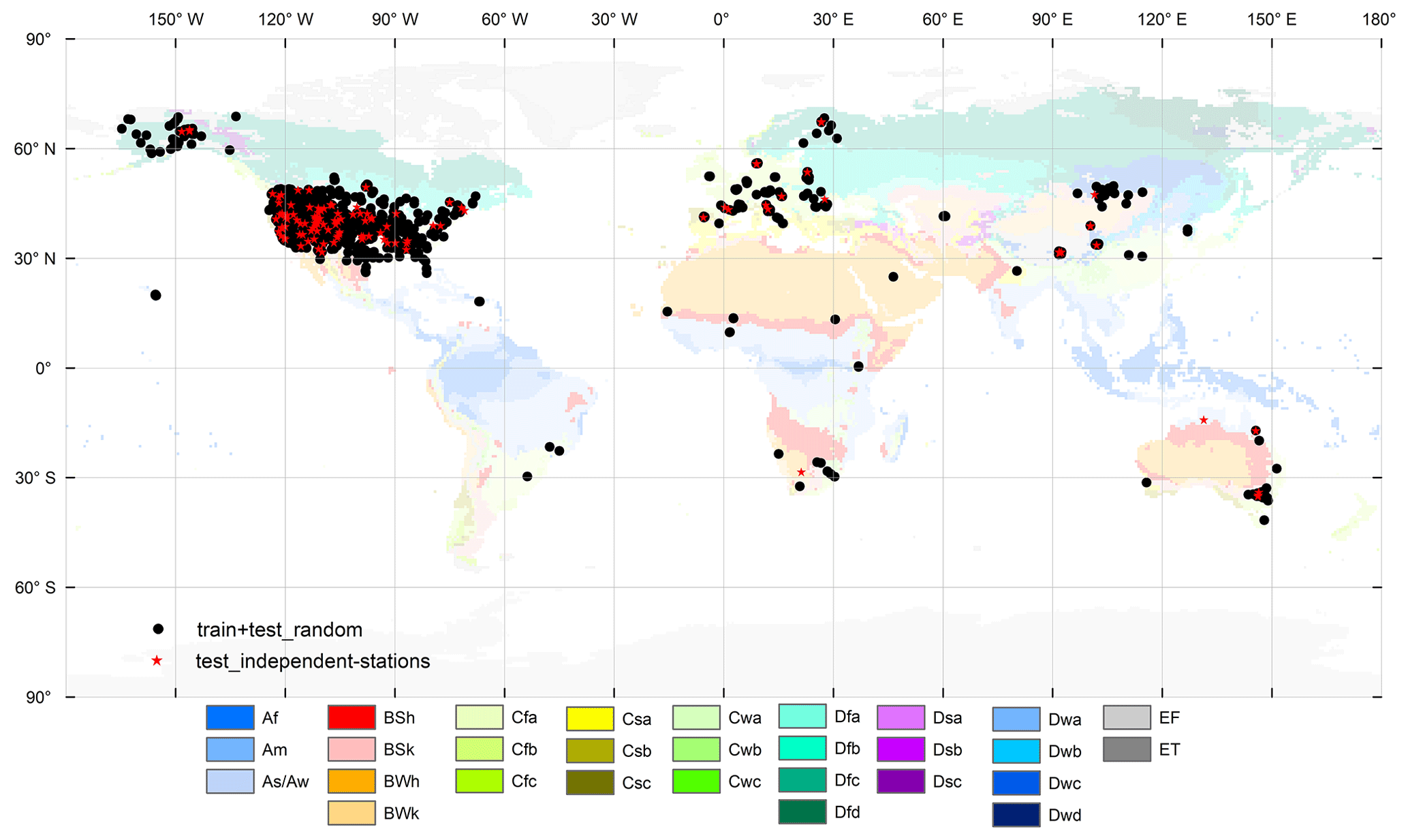
Figure 1 Spatial distribution of the ISMN stations considered in this study and their corresponding climate zones. Note that the data from the 1574 stations coloured in black were used for training and testing the performance of the algorithmic implementations, whereas the 148 stations coloured in red contain independent, unseen data from different locations; the data from the latter stations were used for post-training analysis.

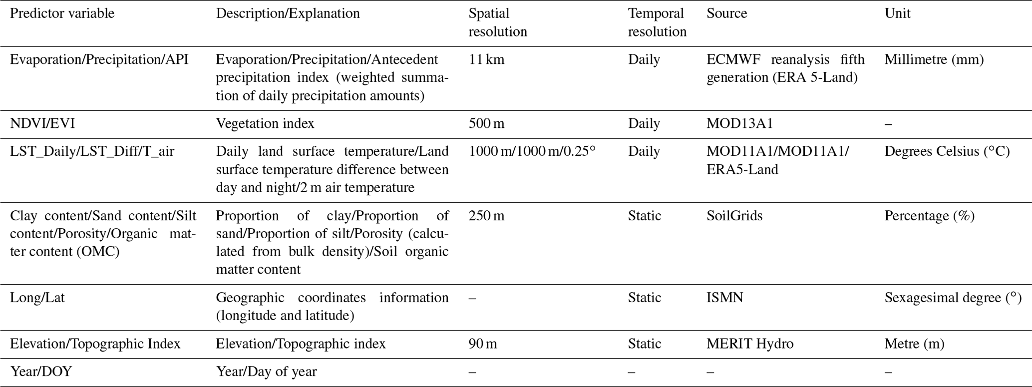
The predictor variables used in the models are listed in Table 1 and detailed hereinafter. The most commonly used predictor variables (e.g. remote-sensing data or reanalysis data) are available on the Google Earth Engine (GEE) platform.

Table 1 Predictor variables used for training the machine learning algorithms.

2.2.1 Precipitation and evaporation

In this study, we used the hourly precipitation and evaporation data from ERA5-Land with a time coverage from 1981 to the present. ERA5-Land is one of the most advanced reanalysis products released by the European Centre for Medium-Range Weather Forecasts (ECMWF), with a higher spatial resolution and better global water balance than ERA-Interim (Albergel et al., 2018; Muñoz-Sabater et al., 2021). To synchronise the temporal coverage of the land surface temperature and vegetation indices, we adopted all precipitation and evaporation data from 2000 to 2018 and aggregated them from hourly into daily values.

2.2.2 Land surface temperature and air temperature

Currently, several LST datasets are available that have been rigorously validated. The MOD11A1 (Collection 6) LST product from the Moderate Resolution Imaging Spectroradiometer (MODIS) is based on the split-window method (Wan, 2014). The spatial resolution of MOD11A1 is 1 km, with two measurements of LST per day – descending at 10:30 LT (local time) and ascending at 22:30 LT, respectively. The MOD11A1 LST was reported with an average error of around 1 ^∘C (Sobrino et al., 2020; Wan, 2014).

2.2.3 Vegetation indices

This study deployed the MOD13A1 dataset of NDVI and EVI from MODIS as the predictor variables (MODIS, 2015). MOD13A1 has a spatial resolution of 500 m and a temporal resolution of 16 d. The selected temporal coverage is the same as for LST (from 1 January 2000 to 31 December 2018).

2.2.4 Soil properties

In this study, the soil texture (proportion of clay, sand, and silt content), bulk density (used for calculating porosity), and organic carbon content (used for calculating organic matter content) values were obtained from SoilGrids (Hengl et al., 2017). The SoilGrids system currently provides the most detailed quantitative information on soil properties at a global scale (Hengl et al., 2017). All soil properties are available for seven respective soil depths: 0, 5, 15, 30, 60, 100, and 200 cm (Hengl et al., 2017; Ross et al., 2018). In this study, clay, sand, and silt content values of the top 5 cm; organic matter content values of the top 5 cm; and bulk density values of the top 5 cm were used.

2.2.5 DEM and the topographic index (TI)

MERIT Hydro was used in this study (Yamazaki et al., 2019).

2.2.6 Köppen–Geiger climate classification

To further investigate the performance of the ML algorithms over different climate conditions, we used the Köppen–Geiger (KG) climate classification system. The KG system classifies the climate based on air temperature and precipitation. The climate is grouped into 5 main classes with 30 sub-types, consisting of tropical, arid, temperate, continental, and polar climates (Beck et al., 2018).

ISMN covers 19 climate zones: Aw – tropical wet and dry or savanna climate, BSh – hot semi-arid climate, BSk – cold semi-arid climate, BWh – hot desert climate, BWk – cold desert climate, Cfa – humid subtropical climate, Cfb – temperate oceanic climate, Csa – hot-summer Mediterranean climate, Csb – warm-summer Mediterranean climate, Cwb – subtropical highland climate, Dfa – hot-summer humid continental climate, Dfb – warm-summer humid continental climate, Dfc – subarctic climate, Dsb – Mediterranean-influenced warm-summer humid continental climate, Dsc – Mediterranean-influenced subarctic climate, Dwa – monsoon-influenced hot-summer humid continental climate, Dwb – monsoon-influenced warm-summer humid continental climate, Dwc – monsoon-influenced subarctic climate, and ET – tundra climate.

2.3 Data preprocessing

2.3.1 Antecedent precipitation index

The ERA5-Land daily precipitation data were used to calculate the antecedent precipitation index (API) (Muñoz-Sabater et al., 2021). The API indicates the reverse-time-weighted summation of precipitation over a specified time (Wilke and McFarland, 1986). The historical precipitation influences the soil water content with a weakening effect along the reverse time axis: more recent rainfall events have a higher impact on the current SSM (Benkhaled et al., 2004).

Many researchers have applied the API to retrieve SSM information (Wilke and McFarland, 1986; Zhao et al., 2011). In this study, we used the API as a feature for the SSM prediction. The definition of API can be represented as follows:

$$\begin{array}{}\text{(1)}& {\mathrm{API}}_a=\sum _{i=\mathrm{0}}^t{k}^i\cdot p_{a-i}.\end{array}$$

In Eq. (1), API_a represents the API value at day a; k is an empirical factor (decay parameter) to indicate the decay effect from the rainfall, which should always be less than 1, with a suggested range of k being between 0.85 and 0.98 (Ali et al., 2010); p_a−i is the precipitation value at the ith day before day a; and t is the number of antecedent days that we used to calculate API_a.

Despite the spatial heterogeneity in the decay parameter (k), as the soil water retention varies in space, most researchers use only one pair of values (k and t) for their study area (Hillel and Hatfield, 2005); this approach was adopted in this work as well. Thus, we calculated the API with different combinations of the parameters (k and t) and compared the corresponding Pearson correlation coefficient (r) of the API and in situ SSM; the final obtained optimised parameters are k=0.91 and t=33.

2.3.2 Reconstruction of the vegetation index

Both the NDVI and EVI from MOD13A1 are MODIS 16 d composite data. Despite an atmospheric correction procedure for the MODIS reflectance data, noise could still be observed in the long-term time series, which is not physical based on plant phenology. Thus, we filtered the NDVI and EVI products with the Savitzky–Golay (S-G) method to reduce the small peak noise (Chen et al., 2004). NDVI and EVI were also interpolated to a daily time step using a simple linear approach to synchronise the temporal steps with other features as follows:

$$\begin{array}{}\text{(2)}& p\left(t\right)=f\left(t\mathrm{0}\right)+\left(f\left(t\mathrm{1}\right)-f\left(t\mathrm{0}\right)\right)\left({\displaystyle \frac{t-t\mathrm{0}}{t\mathrm{1}-t\mathrm{0}}}\right).\end{array}$$

In Eq. (2), p(t) is the interpolated vegetation index; f(t0) and f(t1) are the vegetation index at time t0 and t1, respectively.

2.3.3 Daily LST and daily LST difference

The MOD11A1 LST product consists of two LST values per day (at 10:30 and 22:30 LT) (Wan, 2014). We considered the arithmetic average of them as daily LST and calculated the difference between the daytime and night-time value as the daily LST difference for that day.

The quality of the LST was ensured based on the quality control (QC) data associated with the daytime and night-time LST; only pixels with a QC value of 0 (i.e. good-quality data) were kept (Wan, 2014). The MOD11A1 data used in this study span from 24 February 2000 to 31 December 2018.

2.3.4 Porosity and organic matter content

Soil porosity was derived from Eq. (3), using the bulk density from SoilGrids (Hengl et al., 2017) and particle density:

$$\begin{array}{}\text{(3)}& \mathrm{\varnothing }=\mathrm{1}-{\displaystyle \frac{{\mathit{\rho }}_{\mathrm{b}}}{{\mathit{\rho }}_{\mathrm{s}}}}.\end{array}$$

In Eq. (3), ρ_b is the dry bulk density (g cm⁻³) and ρ_s is the mineral particle density of 2.65 g cm⁻³. For soil mixture, the bulk density scheme assumed that the coarse and fine components share the same particle density.

Soil organic matter content (also retrieved from SoilGrids) can be converted from soil organic carbon content by multiplying by a factor of 1.72 (Khatoon et al., 2017).

2.3.5 DEM and the topographic index (TI)

We used the topographic index of TOPMODEL (Kirkby, 1975), which is defined as follows (Pradhan et al., 2006):

$$\begin{array}{}\text{(4)}& {\displaystyle }\mathrm{TI}=\ln \left({\displaystyle \frac{\mathit{\alpha }}{\mathit{\beta }}}\right);\text{(5)}& {\displaystyle }\mathit{\alpha }={\displaystyle \frac{\mathrm{uca}}{\mathrm{fw}}};\text{(6)}& {\displaystyle }\begin{array}{rl}& \mathrm{fw}=\\ & \left\{\begin{array}{l}\text{90\hspace{0.17em}m when flow direction is 1 or 4 or 16 or 64},\\ \sqrt{\mathrm{90}}\text{ m when flow direction is 2 or 8 or 32 or 128}.\end{array}\right.\end{array}\end{array}$$

Here, TI is the topographic index, α is the ratio of local upslope catchment area (uca) to flow width (fw), and β is the slope angle of the ground surface that can be obtained from elevation data. Upslope catchment area, flow direction, and elevation can be found and used directly from MERIT Hydro: global hydrography datasets (Gruber and Peckham 2009; Yamazaki et al., 2019).

2.3.6 Spatial resampling

Land surface features have different spatial resolutions. For calculating the long-term gridded global SSM, the predictor variables were resampled to a 1 km resolution. Afterwards, the predictor variables were extracted for pixels that collocate with the considered in situ sites, at a 1 km resolution. The World Geodetic System of 1984 (WGS84, EPSG:4326) was chosen as the geographic coordinate system in our study.

2.4 Data split

The precipitation, API, evaporation, air temperature, daily LST, daily LST difference, and NDVI and EVI data (described in Sect. 2.2) were synchronised based on the temporal coverage of in situ data time series of each ISMN station (described in Sect. 2.1). The full data contained a total of 735 475 registries (each sample contained 19 predictor variables) and were differentiated into the training set and three different test sets, based on the following strategy (also described in Table 2):

• First, we extracted 10 % of stations from every network for an independent evaluation of the derived ML models. This is called the “test_independent-stations” set and contains a total of 148 stations. The data from these 10 % of the stations do not belong to the training set nor any test set.

• Afterwards, based on the temporal component of the data, we divided the remaining data (90 % of the full available data) into the “train and test_random” set (containing 70 % of the available data; at this stage, train and test_random form a single temporary set) and the “test_temporal” set (containing 30 % of the available data). This way, assuming the data were recorded from 1 January 2000 to 31 December 2019, the train and test_random set contains the first 70 % of data (14 years, from 2000 to 2013) and the test_temporal set consists of the last 30 % of data (6 years, from 2014 to 2019). The test_temporal set was used to analyse the performance of time series prediction for stations where SSM data from an earlier period were used to build the ML model.

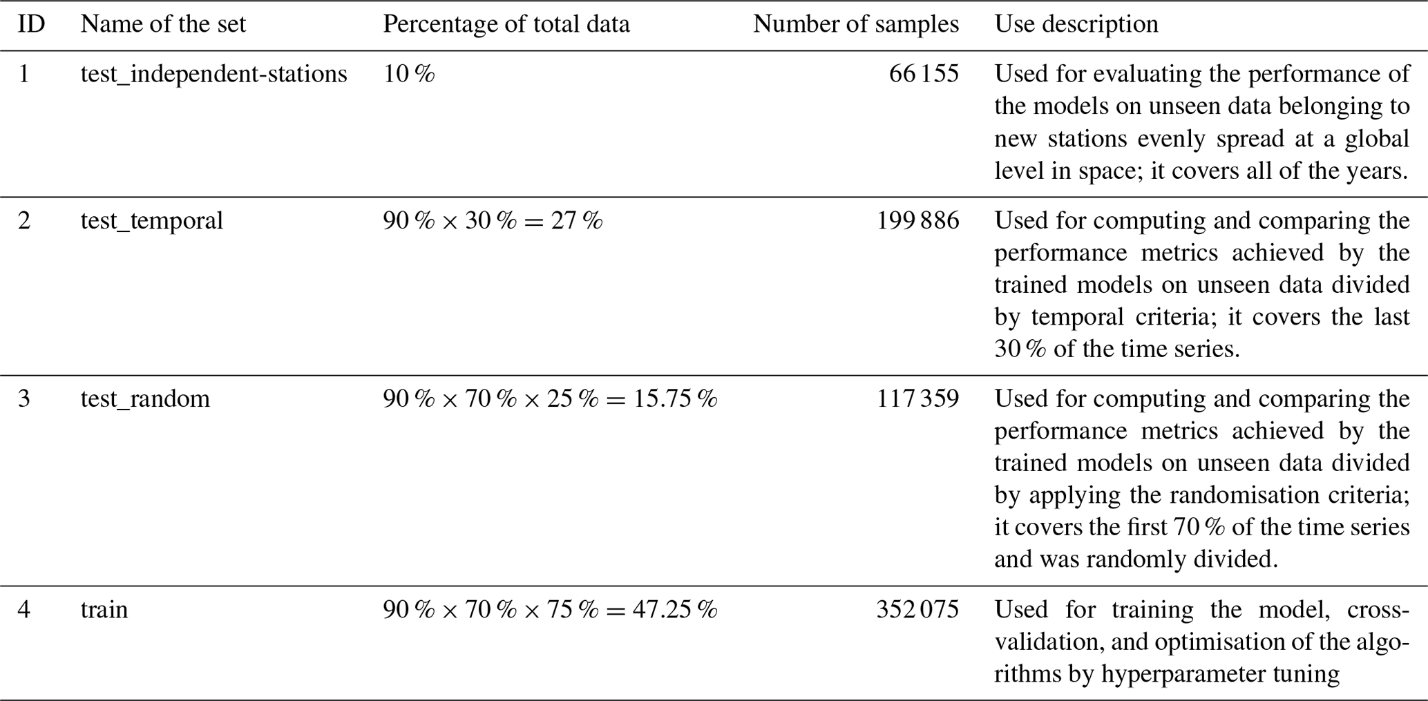
• Finally, the temporary train and test_random data, obtained in the second step, were randomly split into the “train” and “test_random” sets by applying a 75 % to 25 % division criteria. The two resulting sets were used for training and testing the considered algorithmic implementations.

Table 2 Description of the sets of data used for training and testing the machine learning implementations and their size.

3 ML algorithms and ensembles

The optimisation task of the considered ML algorithms involved an extensive search for the training hyperparameters that achieved the highest performance metrics in different training scenarios (as illustrated in Fig. 2).

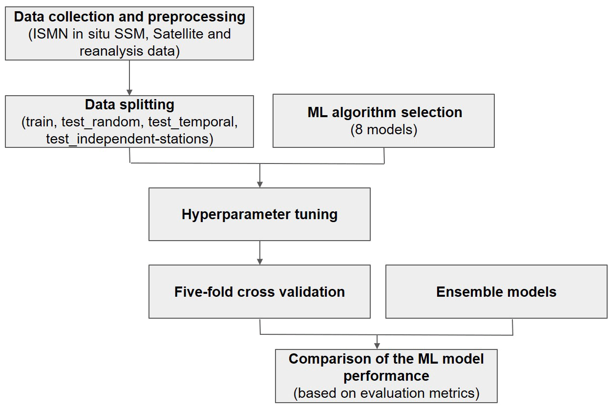
Figure 2 Conceptual framework of the optimisation operation of ML algorithms and the construction of ensemble models.

The data collection and preprocessing step have been explained in Sect. 2.1 and 2.2, while the data-splitting operation has been described in Sect. 2.3. The ML algorithm selection and hyperparameter tuning steps, related to the optimisation procedure, are described in Sect. 3.1 and 3.2. The procedure to build the ensemble models is described in Sect. 3.3. The metrics considered for the comparison are presented in Sect. 3.4. Finally, the comparison of the ML models' performance (either optimised ML models or ensemble models) is approached from different perspectives in Sects. 4 and 5.

3.1 Selection of machine learning algorithms

We used the scikit-learn Python library (Pedregosa et al., 2011) to build and test the machine learning algorithms. Eight algorithms were selected based on their popularity and their proven performance with respect to regression tasks (Sarker, 2021). The algorithms considered for optimisation were (1) Random Forest Regressor (RFR) (Belgiu and Drăguţ, 2016; Breiman, 2001), (2) K-neighbours Regressor (KNR) (Papadopoulos et al., 2011), (3) AdaBoost (AB) (Yıldırım et al., 2019), (4) Stochastic Gradient Descent Regressor (SGDR), (5) Multiple Linear Regressor (MLR), (6) Multi-layer Perceptron Regressor (MLPR) (Gaudart et al., 2004), (7) Extreme Gradient Boosting (XB) (Karthikeyan and Mishra, 2021), and (8) GradientBoosting (GB) (Wei et al., 2019).

3.2 Optimisation procedure (hyperparameter tuning)

Each of the considered eight ML algorithms has different, specific parameters that can be tuned to improve the performance of the prediction. To optimise the training procedure and achieve the maximum performance of the algorithms for our task, we applied the hyperparameter tuning technique (Feurer and Hutter, 2019), as it is one of the most popular methods to search for the best parameter values. In this study, the grid search cross-validation (GridSearchCV) function (LaValle et al., 2004) was implemented in scikit-learn for hyperparameter tuning. In the case of the ML algorithms that require a long computation time, the “itertools” Python function was applied (based on a for loop).

The goal was to identify the best set of specific parameters of the eight considered ML algorithms, with the coefficient of determination r-square (r²) score used as the evaluation metric. In the hyperparameter tuning operation, we set a range for every parameter considered in various iterations. For example, for the “n_neighbors” hyperparameter (specific to the KNR algorithm), we first set the possible values to 5, 10, and 15; after we identified that the best set value is 5, we updated the range of possible values to 3, 4, 5, 6, and 7 to narrow down the possible interval and achieve the parameter values delivering more accurate performance metrics.

3.3 Construction of the ensemble models

In order to enhance capabilities of individual models, we exploited ensemble techniques which helped to identify the proper combination of models. This way, we assembled a set of base models (the optimised versions of machine learning models mentioned in Sect. 3.1, obtained by applying the optimisation procedure described in Sect. 3.2) using model stacking techniques to combine the predictions of the models and built a new model.

The reasoning behind using an ensemble was as follows: by stacking multiple base models representing different hypotheses, we can find a better hypothesis that might not be contained within the hypothesis space of the individual models from which the ensemble is built (Cira et al., 2020). Three main aspects causing this situation were identified (Dietterich, 2000): (1) insufficient input data (statistical), (2) difficulties for the learning algorithm to converge to the global minimum (computational), and (3) the function cannot be represented by any of the hypotheses proposed nor modelled by the algorithms during training (representational).

A popular form of stacking involves computing the outputs of base models, performing a prediction for each model, and averaging their predictions inside the ensemble. In this technique, each m sub-model contributes equally to a combined prediction, y, as defined in Eq. (7). The specific steps are as follows: (1) generate weak learners, each with its own initial values (by training them separately), and (2) combine these models in an ensemble environment, where their predictions are averaged for every instance of the set to compute.

$$\begin{array}{}\text{(7)}& \stackrel{\mathrm{‾}}{y}\left(x\right)={\displaystyle \frac{\mathrm{1}}{M}}{\sum }_{m=\mathrm{1}}^M{y}_m\left(x\right)\end{array}$$

We built ensemble models by combining base models as diversely as possible (an example is illustrated in Fig. 3). This way, the optimised versions of single ML algorithms become the weak learners, or base models, within ensemble models that will be constructed using model bagging methodology. We applied ensemble learning procedures to test different combinations of the algorithms with the highest performance metrics and study their impact on the predictive performance.

The base models are the five ML models that achieved the highest performance metrics after the optimisation procedure described in Sect. 3.2. The constructed ensemble model variants will contain all of the possible combinations of the five base models, taken three at a time ($C_n^k=\frac{n\mathrm{!}}{k\mathrm{!}\left(n-k\right)\mathrm{!}}$, where n=5, k=3). In this way, 10 ensemble models will be obtained, and the performance of every ensemble model built will be studied in Sect. 4.3.2.

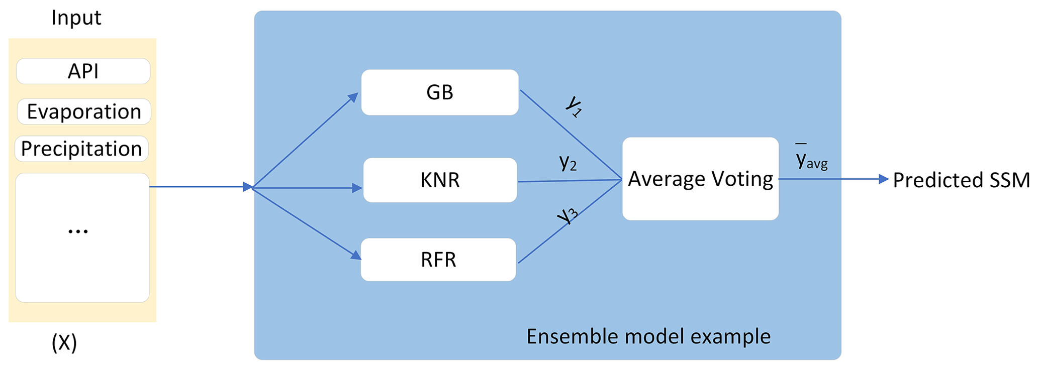
Figure 3 Example of an ensemble model structure (based on the average voting of three weak learners).

3.4 Evaluation of the performance

We use five-fold cross validation to evaluate the training performance of different algorithms, both before and after the hyperparameter tuning.

To assess the performance of different ML algorithms, we compared predicted SSM with in situ observations. In this research, we considered three commonly used statistical evaluation metrics (Entekhabi et al., 2010b): the root-mean-square error (RMSE), defined in Eq. (8); the Pearson correlation coefficient (r) score, represented in Eq. (9); and the coefficient of determination r-square (r²) score, presented in Eq. (10).

$$\begin{array}{}\text{(8)}& {\displaystyle }\mathrm{RMSE}=\sqrt{{\displaystyle \frac{{\sum }_{i=\mathrm{1}}^N(y_{\mathrm{pred},i}-y_{\mathrm{ref},i}{)}^{\mathrm{2}}}{N}}}\text{(9)}& {\displaystyle }r={\displaystyle \frac{{\sum }_{i=\mathrm{1}}^N(y_{\mathrm{pred},i}-\stackrel{\mathrm{‾}}{y_{\mathrm{pred},i}})(y_{\mathrm{ref},i}-\stackrel{\mathrm{‾}}{y_{\mathrm{ref},i}})}{\sqrt{{\sum }_{i=\mathrm{1}}^N(y_{\mathrm{pred},i}-\stackrel{\mathrm{‾}}{y_{\mathrm{pred},i}}{)}^{\mathrm{2}}}\sqrt{{\sum }_{i=\mathrm{1}}^N(y_{\mathrm{ref},i}-\stackrel{\mathrm{‾}}{y_{\mathrm{ref},i}}{)}^{\mathrm{2}}}}}\text{(10)}& {\displaystyle }{r}^{\mathrm{2}}=\mathrm{1}-{\displaystyle \frac{{\sum }_{i=\mathrm{1}}^N(y_{\mathrm{ref},i}-y_{\mathrm{pred},i}{)}^{\mathrm{2}}}{{\sum }_{i=\mathrm{1}}^N(y_{\mathrm{ref},i}-\stackrel{\mathrm{‾}}{y_{\mathrm{ref},i}}{)}^{\mathrm{2}}}}\end{array}$$

In Eqs. (8) to (10), y_pred,i is the predicted SSM, y_ref,i is the in situ SSM, N is the number of valid pairs of SSM, $\stackrel{\mathrm{‾}}{y_{\mathrm{pred},i}}$ is the mean value of the predicted SSM, and $\stackrel{\mathrm{‾}}{y_{\mathrm{ref},i}}$ is the mean value of the in situ SSM.

In this study, there are three main steps: (1) the evaluation of the r² score on the training set; (2) the evaluation of the five-fold cross validation; and (3) the evaluation of the test_random, test_temporal, and test_independent-stations sets. In the first step of the evaluation, the r² score on the training dataset was analysed to identify significant differences among different ML algorithms. In the second step, the r² score and RMSE were computed to carry out the performance comparison on the train set using cross validation. In the third step, the r score, r² score, and RMSE were calculated on the test_random, test_temporal, and test_independent-stations sets to compare the performance of the trained algorithms.

The performance of the 8 ML algorithms and 10 ensemble models were compared with respect to the squared error of the predictions using a non-parametric Kruskal–Wallis test at the 5 % significance level, computed on the test_random, test_temporal, and test_independent-stations sets.

4 Results

4.1 Best parameters from hyperparameter tuning (optimised machine learning models)

The optimal performance after the hyperparameter tuning is presented in the fourth column of Table S1 in the Supplement. The RFR, KNR, and XB algorithms show a superior result with r² scores of 0.859, 0.8848, and 0.9139, respectively, while the GB, MLPR, and AB algorithms also show a considerable result with r² scores of 0.7977, 0.7638, and 0.6547, respectively. It should be noticed that, in other relevant studies, such as Kucuk et al. (2022), AB also performed slightly worse than RFR, GB, and XB with respect to SSM estimation. However, the performance of the other two methods (SGDR and MLR) is not satisfactory. Both SGDR and MLR were unable to model the highly non-linear relationship between the soil moisture and the predictor variables because these two algorithms are linear regressors.

The computational efficiency of hyperparameter tuning of different algorithms varies greatly, sometimes with a different order of magnitude. For example, it only took 17 min for GB to finish the turning, whereas XB needed more than 25 h. However, this seems to be more dependent on the choice of parameters and their range, as XB has nine parameters, and we selected at least five values to tune for each parameter.

4.2 Five-fold cross validation

After hyperparameter tuning, five-fold cross validation was used for performance comparison on the train dataset. The performance of the five-fold cross-validation for the eight algorithms is listed in Table 3. Similar to the result in Table S1, five algorithms (RFR, KNR, MLPR, XB, and GB) display a high performance. XB achieved the best performance, with an RMSE of 0.0337 cm³ cm⁻³ and an r² score of 0.9081. It is followed by the KNR algorithm, with an RMSE of 0.0392 cm³ cm⁻³ and an r² score of 0.8760. RFR, GB, and MLPR also achieved acceptable performance, even though an RMSE of 0.04 cm³ cm⁻³ is often required in the community as a non-strict standard.

Table 3 Mean values and standard deviation of the evaluation metrics obtained in the five-fold cross validation.

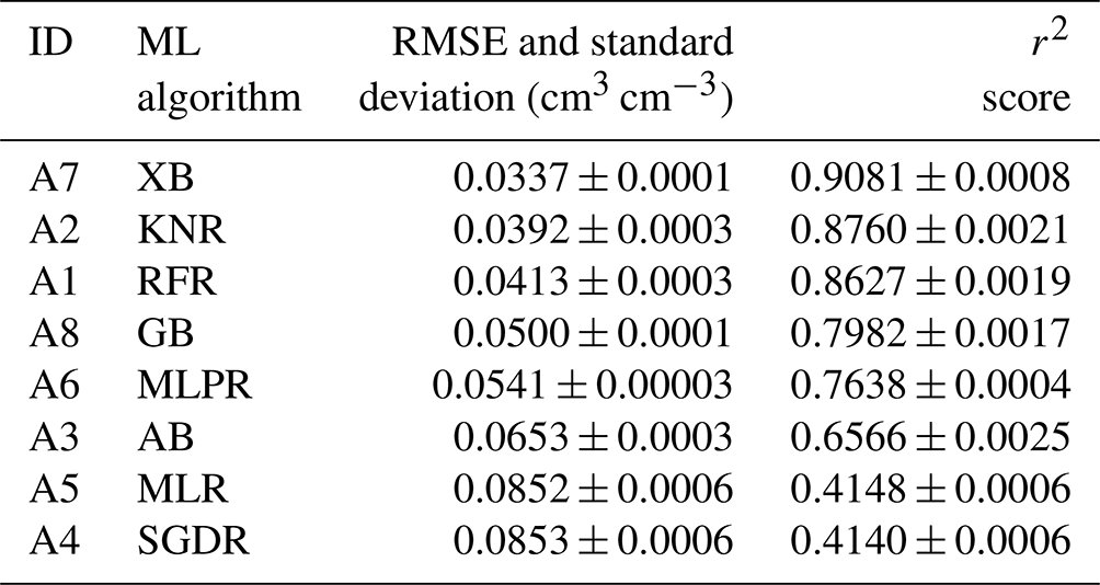
The abbreviations used in the table are as follows: XB – Extreme Gradient Boosting, KNR – K-neighbours Regressor, RFR – Random Forest Regressor, GB – GradientBoosting, MLPR – Multi-layer Perceptron Regressor, AB – AdaBoost, MLR – Multiple Linear Regressor, and SGDR – Stochastic Gradient Descent Regressor.

4.3 Analysis of the model performance on the test_random, test_temporal, and test_independent-stations sets

4.3.1 Performance of single, optimised ML models

Having identified the best hyperparameters for the considered algorithms and, therefore, the optimised versions of the ML models for our task, we next calculated and compared their performance on the test_random, test_temporal, and test_independent-stations sets. As described in Table 2, the number of samples used to evaluate the performance (each containing 19 predictor variables) for the train, test_random, and test_temporal sets were 352 075, 117 359, and 199 886 registries, respectively, together with 148 stations in the test_independent-stations set (containing 66 155 registries). The number of stations was 1574 for the train and test_random sets and 1550 for the test_temporal set.

From Table 4, we can find that RFR, KNR, and XB performed better on the test_random set, compared with the other five algorithms. KNR achieved the best performance, with a maximum r² score of 0.8848. RFR, KNR, AB, XB, GB, and MLPR performed relatively well on the test_temporal set, achieving a maximum r² score of 0.7126. In independent station evaluation, except MLPR, all ML algorithms perform similarly, but AB performs the best (with an r² score of 0.4905). Overall, RFR, KNR, and XB performed well at every step.

Table 4 Performance metrics obtained by eight optimised ML algorithms on the test sets.

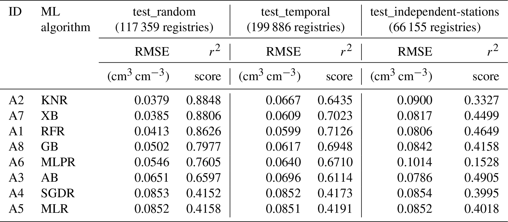
The abbreviations used in the table are as follows: KNR – K-neighbours Regressor, XB – Extreme Gradient Boosting, RFR – Random Forest Regressor, GB – GradientBoosting, MLPR – Multi-layer Perceptron Regressor, AB – AdaBoost, SGDR – Stochastic Gradient Descent Regressor, and MLR – Multiple Linear Regressor.

4.3.2 Performance of ensemble models

Based on the results displayed in Table 4, the ensemble regressors were built using RFR, KNR, XB, GB, and AB as base models (as they displayed the best performance). We integrated three ML algorithms in each combination to form the 10 ensemble models. The performance of these 10 models was found to be stable (as observed in Table 5). Specifically, KNR_RFR_ XB and GB_RFR_XB displayed the best performance in test_random (the RMSE values were 0.0355 and 0.0391 cm³ cm⁻³ and the r² scores were 0.8985 and 0.8772) and test_temporal (the RMSE values were 0.0576 and 0.0568 cm³ cm⁻³ and the r² scores were 0.7335 and 0.7410) sets. However, there were no considerable differences among the different combinations for test_independent-stations.

The voting regressors built with ensemble techniques generally showed improved performance when compared with the considered base models. For example, AB achieved an RMSE of 0.0651, 0.0696, and 0.0786 cm³ cm⁻³ for the test_random, test_temporal, and test_independent-stations sets, respectively, while in the voting regressor result, the six combinations that had AB were able to achieve RMSE values of 0.0417 to 0.0468 cm³ cm⁻³ for the test_random set, 0.0584 to 0.0593 cm³ cm⁻³ for the test_temporal set, and 0.0767 to 0.0775 cm³ cm⁻³ for test_independent-stations set. The ensemble models improved AB's performance by 0.0183–0.0234 cm³ cm⁻³ (28 %–36 %), 0.0103–0.0112 cm³ cm⁻³ (15 %–16 %), and 0.0011–0.0019 cm³ cm⁻³ (1.4 %–2.4 %) for the test_random, test_temporal, and test_independent-stations sets in terms of the RMSE.

The best-performing voting regressor (KNR_RFR_XB, composed of XB, RFR, and KNR) achieved an RMSE value of 0.0355 cm³ cm⁻³ and an r² score value of 0.8985 on the test_random set. The RMSE values of KNR, RFR, and XB were 0.0379, 0.0413, and 0.0385 cm³ cm⁻³ for the test_random set, respectively, and the r² scores of KNR, RFR, and XB were 0.8848, 0.8626, and 0.8806, respectively. Compared with KNR, RFR, and XB, the performance of the ensemble model KNR_RFR_XB was improved; for example, for RFR, the performance was improved by 0.0058 cm³ cm⁻³ (14 %) for the RMSE and by 0.0359 (4 %) for the r² score. On the test_temporal and test-independent-stations sets, the performance of KNR_RFR_XB was also better than the single three ML algorithms. In summary, models built with ensemble techniques averaged the performance of base ML algorithms and performed more stably than single ML algorithms. Overall, ensemble techniques improved the performance of base algorithms for the test_random dataset, but they had little effect on the test_independent-stations dataset.

Table 5 Performance metrics obtained by the 10 ensemble models built with different combinations of selected machine learning algorithms.

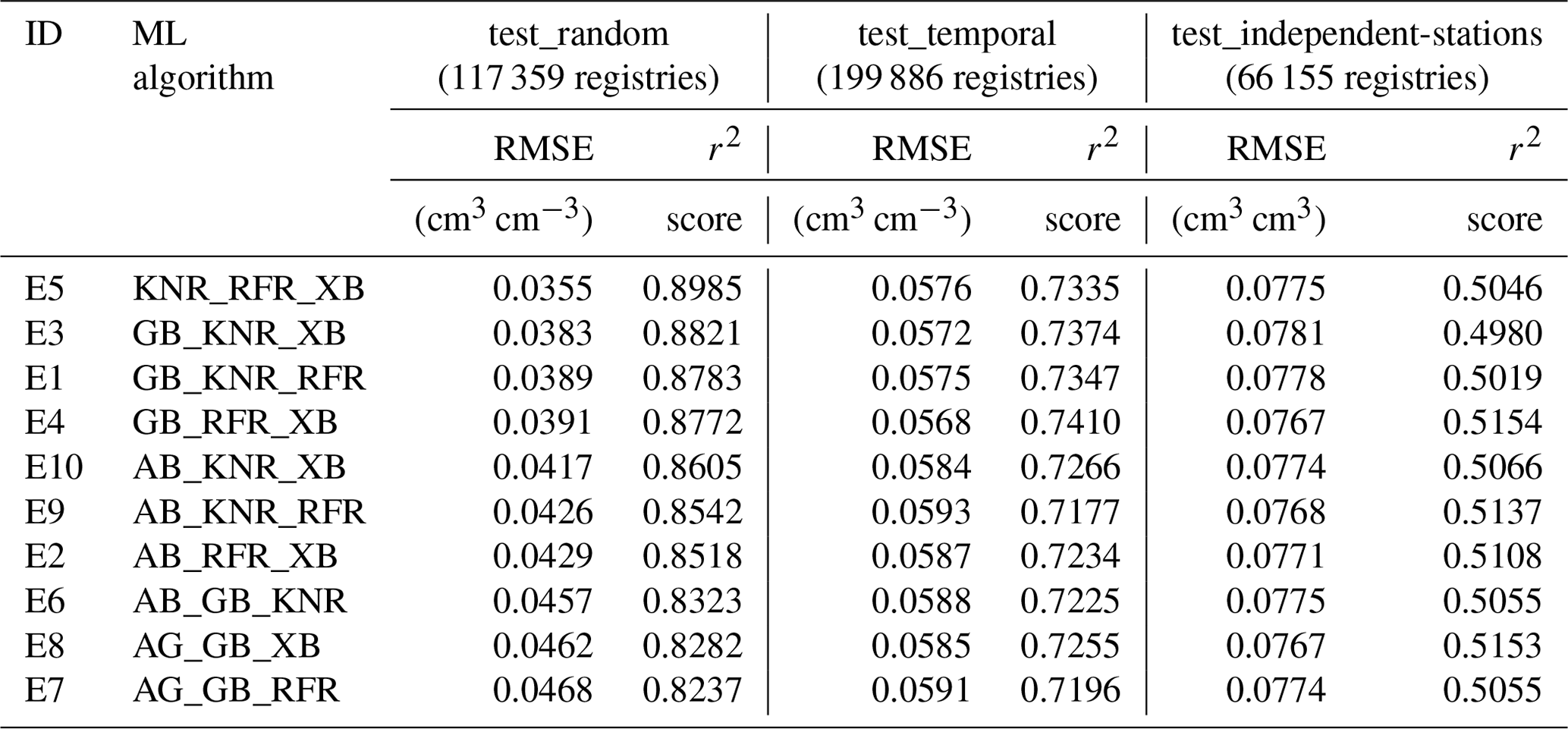
The abbreviations used in the table are as follows: RFR – Random Forest Regressor, KNR – K-neighbours Regressor, AB – AdaBoost, XB – Extreme Gradient Boosting, and GB – GradientBoosting. Note that GB_KNR_ RFR refers to the ensemble model constructed by GB, KNR, and RFR, whereas AB_RFR_XB refers to the ensemble model constructed by AB, RFR, and XB. The same naming procedure applies for GB_KNR_XB, GB_RFR_XB, KNR_RFR_XB, AB_GB_KNR, AB_GB_RFR, AB_GB_XB, AB_KNR_RFR, and AB_KNR_XB.

4.3.3 Comparison of single, optimised ML and ensemble models

Table 6 shows which methods performed significantly better or worse and the cumulative rank of the methods based on the Kruskal–Wallis order computed for the three test sets. Based on the analysis on the test_random set, KNR is significantly more accurate than the other methods. The ensembles comprising KNR with RFR and XB, with RFR and GB, or with GB and XB are the second, third, and fourth most accurate methods, respectively. When the performance of single algorithms is considered, RFR, XB, and GB follow the performance of KNR. MLR and SGDR display the weakest performance. If AB, which has weaker performance than a single ML, is assembled with KNR, XB, or RFR – which are all significantly more accurate than AB – the prediction performance of the ensemble significantly decreases compared with the performance of those single algorithms. GB, MLPR, AB, SGDR, and MLR describe the relationship between the target and predictors significantly less accurately than the ensemble methods.

For the test_temporal set, KNR_RFR_XB performs significantly better than any of the other methods. The ensembles of GB with KNR and XB, with KNR and RFR, or with RFR and XB are the second, third, and fourth most accurate methods, respectively. Among the single ML methods, RFR is significantly the most accurate, followed by KNR, XB, GB, and MLPR. Similarly to the results for the test_random set, MLR and SGDR performed significantly worse compared with any other method. If an ensemble of AB with KNR or RFR is used, the predictive performance does not improve significantly or significantly decreases compared with the performance of those single ML algorithms.

For the test_independent-stations set, the best-performing predictions could be reached using the ensemble of any three ML algorithms from KNR, RFR, XB, and GB. Among the single, optimised ML methods, RFR is significantly more accurate, followed by XB, AB, GB, KNR, MLR, SGDR, and MLPR. All ensembles perform significantly better than the single ML algorithms.

The results underpin that the inclusion of an algorithm that is not performing well in an ensemble will lead to worse performance than a single model that is performing well.

Table 6 Result of the Kruskal–Wallis test.

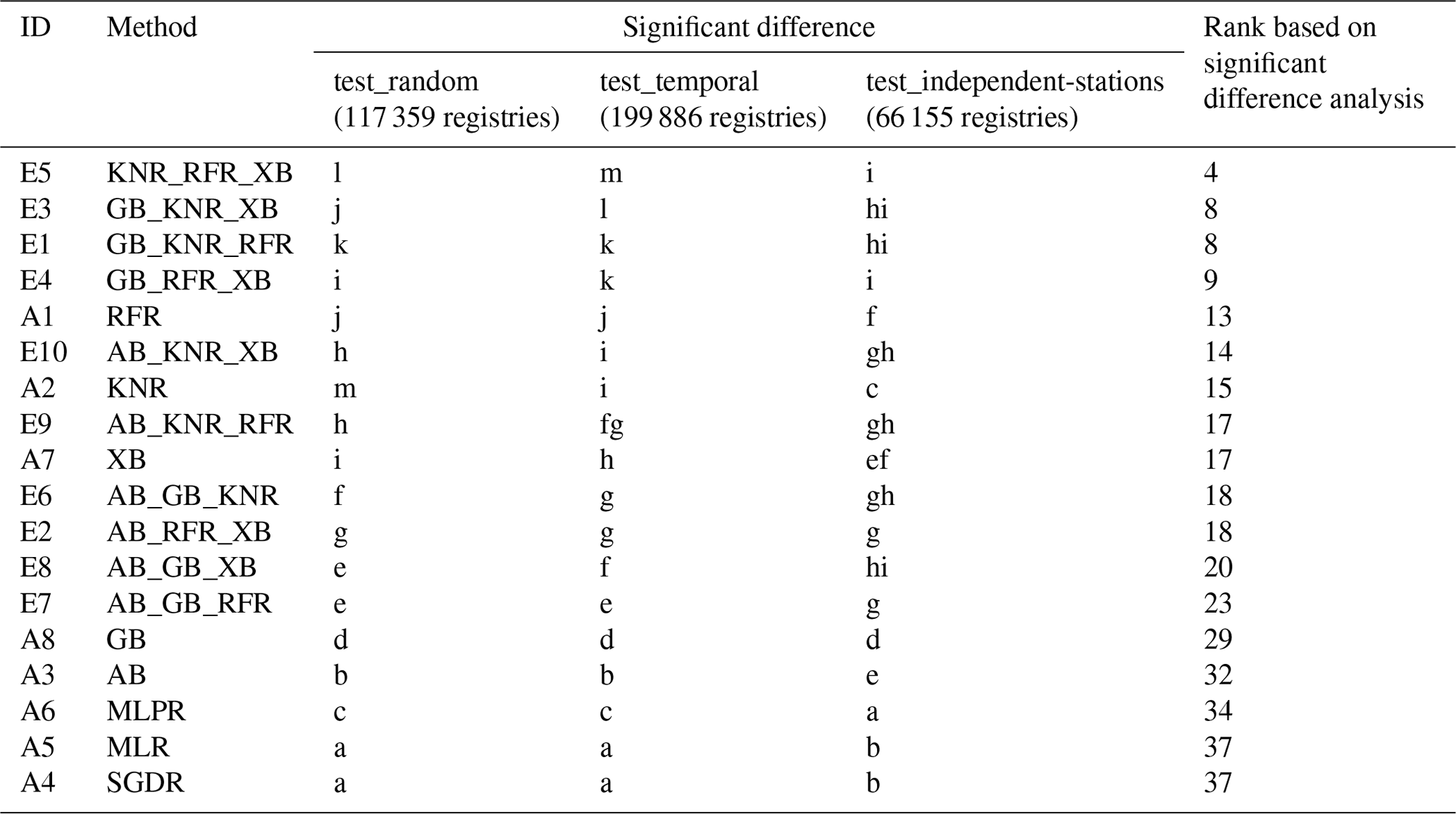
Note that the different letters show that there is a significant difference between the methods. The letter “a” indicates the worst-performing algorithm.

Based on the result of the Kruskal–Wallis test, the best single ML and the best ensemble algorithms were identified. Their probability density functions (PDFs) are shown in Fig. S4 in the Supplement. For the test_random set, the overlap between the in situ SSM and predicted SSM from KNR and KNR_RFR_XB is 96.2  and 93.1 %, respectively. For the test_temporal set, the overlap between the in situ SSM and predicted SSM from RFR and KNR_RFR_XB is 87.9  and 90.7 %, respectively. For the test_independent-stations set, the overlap between the in situ SSM and predicted SSM from RFR and KNR_RFR_XB is 80.5 and 81.0 %, respectively. This shows that the ensemble model performs better on unseen data.

4.4 Performance on the test_independent-stations set grouped by climate zones

In Sect. 4.3, we analysed the performance of our model on three sets, test_random, test_temporal, and test_independent-stations, which consist of stations located in different climate zones; as expected, we observed important variations in the model's performance across different stations (due to their unique climatic conditions).

To further examine the performance of each station in the test_independent-stations set, we considered the number of stations in both the train and test_independent-stations sets. Specifically, the stations from the train set are distributed across 19 Köppen climate zones, whereas the test_independent-stations set stations are across 16 climate zones (Cwb, Dsc, and Dwb, are not represented in the test_independent-stations set).

To ensure a robust climate zone analysis, we excluded stations with less than 100 d of observations in the test_independent-stations set. Figure S2 shows the number of stations in the test_independent-stations dataset over each climate zone; the number of stations decreased from 148 to 117 after applying the (100 d) filter, and the climate zones covered by test_independent-stations set decreased from 16 to 15 (Dwc was removed).

The performance of the 8 optimised ML algorithms and 10 constructed ensemble models in the 15 climate zones is described in the box plots of Fig. 4 (which includes the stations from the test-independent-stations set with more than 100 d of in situ measurements). In Fig. 4a, the median RMSE values in most of the climate zones were below 0.1 cm³ cm⁻³. In Fig. 4b, in 13 climate zones (excluding BSh and BWh), we find at least one single ML algorithm with a median r score higher than 0.6. GB, MLPR, SGDR, and RFR can achieve a median r score of 0.6 in 12, 11, 9, and 9 climate zones, respectively. The median r scores from GB in BSh, BWh, and BWk were below 0.6 because these three climate zones all have sparse train stations and are all arid. In Fig. 4c, the median RMSE values in all climate zones were below 0.075 cm³ cm⁻³ for ensemble models. From Fig. 4d, we can see that the r scores in the other 13 climate zones were above 0.6 (excluding BSh and BWh). This indicates that the number of train stations also plays an important role in ensemble models. Ensemble models can improve performance but can not completely solve the problem of lacking training data.

Using ensemble models is a way to improve the performance of the single, optimised ML algorithms. However, the outliers in the lower part of the r score box plot were still present in BSk and Dfb, even for the ensemble models.

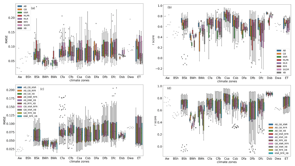
Figure 4 Box plot of the RMSE and r score for the test_independent-stations set based on climate zones: the performance of 8 optimised ML algorithms can be found in panels (a) and (b), while the performance of 10 ensemble models are shown in panels (c) and (d). The abbreviations used in the figure for the climate zones are as follows: Aw – tropical wet and dry or savanna climate, BSh – hot semi-arid climate, BSk – cold semi-arid climate, BWh – hot desert climate, BWk – cold desert climate, Cfa – humid subtropical climate, Cfb – temperate oceanic climate, Csa – hot-summer Mediterranean climate, Csb – warm-summer Mediterranean climate, Dfa – hot-summer humid continental climate, Dfb – warm-summer humid continental climate, Dfc – subarctic climate, Dsb – Mediterranean-influenced warm-summer humid continental climate, Dwa – monsoon-influenced hot-summer humid continental climate, and ET – tundra climate. The abbreviations used in the figure for the ML algorithms are as follows: RFR – Random Forest Regressor, KNR – K-neighbours Regressor, AB – AdaBoost, SGDR – Stochastic Gradient Descent Regressor, MLR – Multiple Linear Regressor, MLPR – Multi-layer Perceptron Regressor, XB – Extreme Gradient Boosting, and GB – GradientBoosting. Note that GB_KNR_RFR refers to the ensemble model constructed by GB, KNR, and RFR, whereas AB_RFR_XB refers to the ensemble model constructed by AB, RFR, and XB. The same naming procedure applies for GB_KNR_XB, GB_RFR_XB, KNR_RFR_XB, AB_GB_KNR, AB_GB_RFR, AB_GB_XB, AB_KNR_RFR, and AB_KNR_XB.

4.5 Performance on single, selected stations from the test_independent-stations set

We selected the BSk climate zone as an example to deepen the analysis of outliers. The weakest r scores were present at Sevilleta station (34.36^∘ N, 106.68^∘ W), with the r scores all being lower than 0.4 for each of the 8 single, optimised ML algorithms and the 10 ensemble models.

For our single-station analysis, we also chose two stations where the performance values were improved by the ensemble models. In Fig. 7, we can observe that all r scores computed for the ensemble models at Carrizoran station (35.28^∘ N, 120.03^∘ W; climate zone BSk) were above 0.8, while all r scores were above 0.6 at Whiskeyck station (37.21^∘ N, 105.12^∘ W; climate zone BSk).

In Fig. 6, it can be found that the predicted SSM was consistent with the in situ SSM at both of these stations. For the outlier station, Sevilleta, we found that the r score between API and predicted SSM is 0.8, whereas the r score between evaporation and predicted SSM is −0.67. This implied that our predictor variables were consistent with our predicted SSM, but the predictor variables were not the main decisive factor for the in situ SSM at station Sevilleta. There was no significant difference between the main static predictor variables of Sevilleta station and other stations in the BSk climate zone. The potential cause could be an environmental factor that is not considered to be an independent variable during the prediction (e.g. different vegetation types).

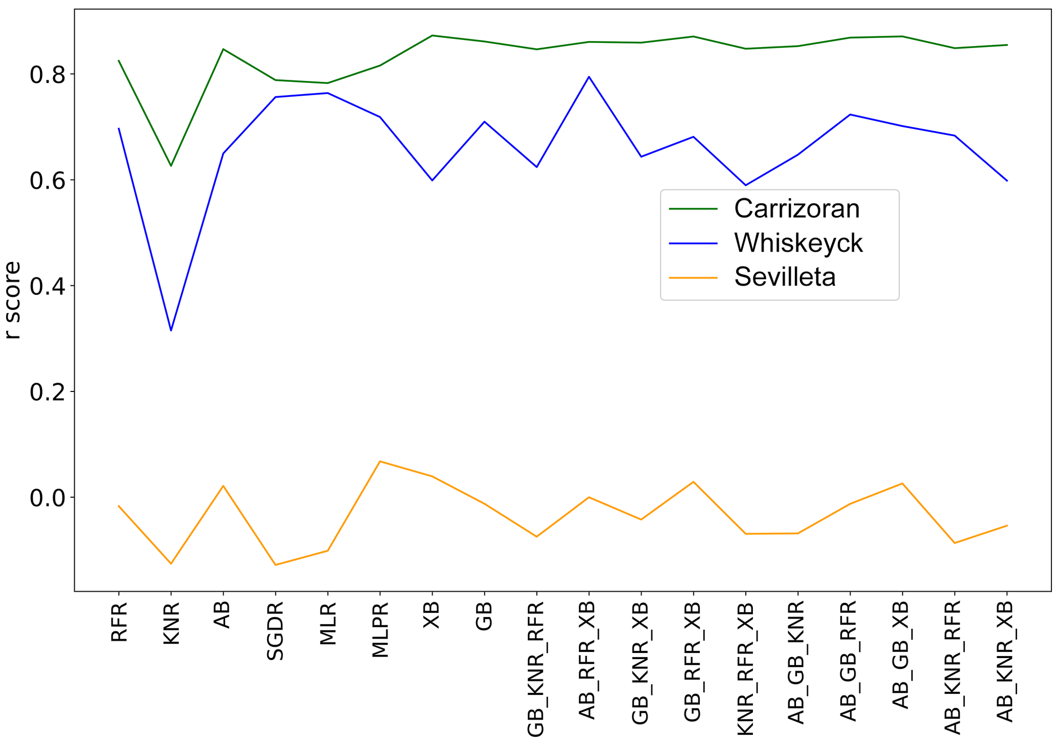
Figure 5 The r scores of three stations obtained by 8 optimised ML algorithms and 10 ensemble models.

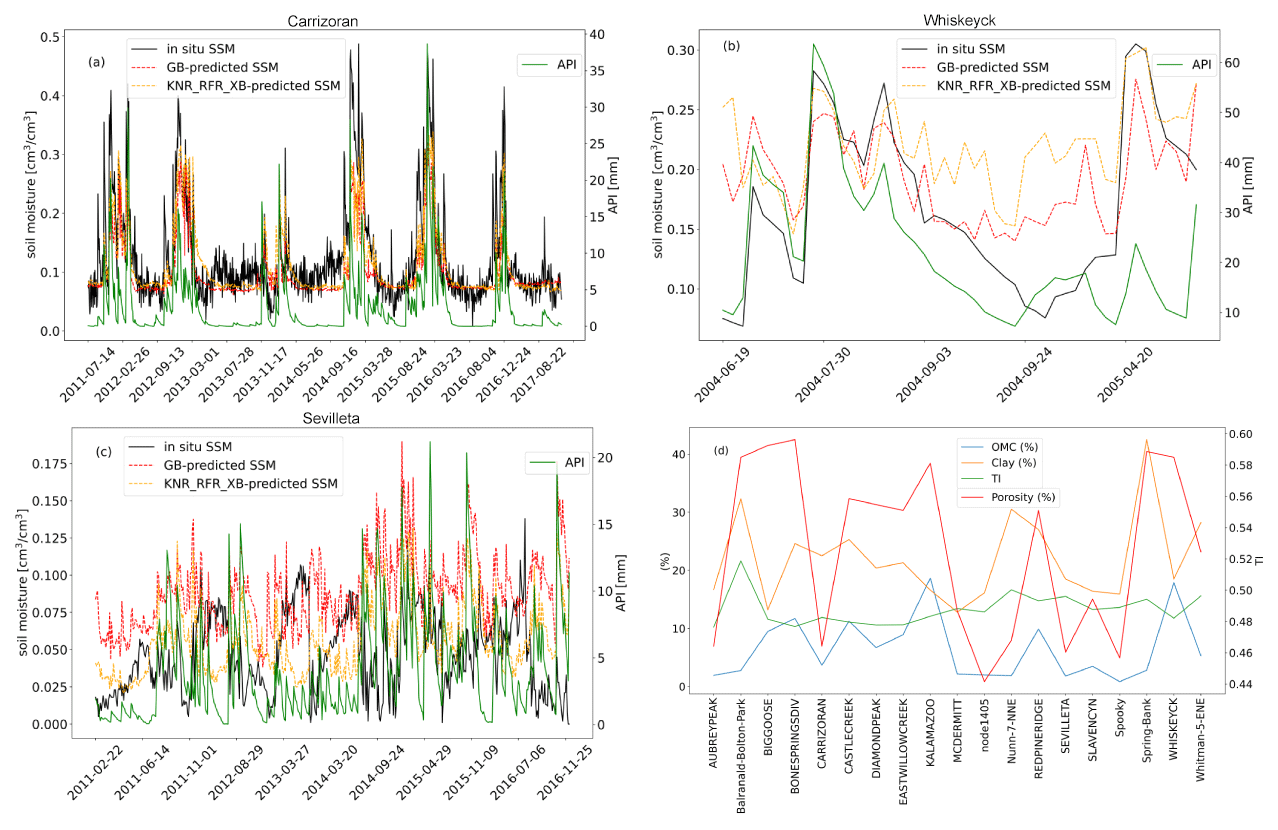
Figure 6 In situ and predicted SSM from GB and KNR_RFR_XB and the API at the (a) Carrizoran, (b) Whiskeyck, and (c) Sevilleta stations; panel (d) presents static predictors of stations in climate zone BSk.

5 Discussion

Soil moisture is an important parameter for understanding the water cycle, predicting crop yields, and managing irrigation. Remotely sensed soil moisture has become an important dataset with respect to supporting many human activities, such as water resource conservation and management, environmental monitoring, and disaster response (Su et al., 2003). In this section, we will discuss the performance and the uncertainty of single, optimised ML algorithms and the proposed ensemble models.

5.1 Performance of trained regression models

This study presents one of the first studies constructing and comprehensively evaluating different ML algorithms for estimating SSM with not only optimised, individual models but also with ensemble models using the optimised algorithms as base models. The predictor variables were selected based on their relevance to physical processes in land–atmosphere interaction.

First, based on various predictor variables extracted from multi-source datasets, we trained and tested 18 ML models in order to find their optimised version for estimating SSM. The cross-validation result showed that RFR, KNR, and XB outperform other ML algorithms. When evaluated on the test_random set, KNR achieved the lowest RMSE (0.0379 cm³ cm⁻³) among individual ML algorithms and a high r² score (0.8848). In contrast, for the test_temporal set, RFR showed the lowest RMSE (0.0599 cm³ cm⁻³) and highest r² score (0.7126). For the test_independent-stations set, AB showed the lowest RMSE (0.0786 cm³ cm⁻³) and highest r² score (0.4905).

Second, the ensemble models improved the performance of the individual ML algorithms if the ensemble did not include a significantly worse-performing algorithm. From Sect. 4.3.2, we can observe that ensemble models mostly improved the performance of base algorithms in the test_random set and had a minimal impact on the test_independent-stations set. From Sect. 4.3.3, it can be noted that the ensemble models based on the combination of KNR_RFR_XB showed the best performance on the test_random and test_temporal sets. KNR_ RFR_XB and GB_RFR_XB had significantly better performance on the test_independent-stations set. Considering the performance of all 8 ML algorithms and 10 ensembles on all three test sets, the ensemble of KNR and RFR and XB performs the best; thus, this is the suggested method to predict SSM based on the presented predictors.

Third, we found significant variations in the model's performance across different stations because of their unique climatic conditions. Therefore, we further analysed the test_independent-stations performance on the climate zone level. For single, optimised ML algorithms, the median RMSE values from five models (excluding MLPR, MLR, and SGDR) were below 0.1 cm³ cm⁻³. GB, XB, and RFR achieved a median r score of 0.6 in 12, 11, and 9 climate zones, respectively, out of 15 climate zones. The ensemble models significantly improved the performance. The median RMSE values in all climate zones were below 0.10 cm³ cm⁻³, and all voting regressors achieved r scores above 0.6 in 13 climate zones (excluding BSh and BWh because of the sparse distribution of train stations).

Fourth, we selected the BSk climate zone as an example to deepen the analysis of outlier stations. The result showed that ensemble models can improve the performance of single ML algorithms and obtain more stable results. The r scores from ensemble models at the Carrizoran station were all above 0.8 and those at the Whiskeyck station were all above 0.6; in general, the optimised individual ML algorithms did not perform as well as the ensemble models. However, we found the worst performance at the outlier station, Sevilleta, and the ensemble models could not improve this performance. The potential cause could be an environmental factor that is not considered as an independent variable during the prediction (e.g. different vegetation types). Another potential cause could be the non-representativeness of the in situ measurements for the studied pixel scale.

When considering ensemble models, there are several advantages. Firstly, the ensemble models significantly improve the accuracy of the individual ML algorithms. By combining multiple regression models, the ensemble models can capture more of the complexity and variability in the data, leading to more accurate predictions (Cira et al., 2020). Secondly, because the ensemble models uses multiple models, they are less sensitive to outliers or individual model errors, making them more robust and stable models. Thirdly, the ensemble models allow us to use different types of regression models and hyperparameters, so researchers can choose the best models for their particular data and problem. Lastly, the ensemble models can reduce overfitting by combining models that have different strengths and weaknesses, leading to a more generalisable model. Furthermore, a comparison of ensemble models with other existing soil moisture products and methods highlights their superior performance. For instance, evaluating the root-mean-square error (RMSE) on randomly selected test samples, our KNR_RFR_XB ensemble model achieves an RMSE of 0.0355 cm³ cm⁻³. In contrast, the RFR model used to generate a global daily 1 km soil moisture product presents an ubRMSE (unbiased root-mean-square error) of 0.045 cm³ cm⁻³ (Zheng et al., 2023), and the RFR model used to generate a global daily 0.25^∘ soil moisture product presents an RMSE of 0.05 cm³ cm⁻³ (Zhang et al., 2021). The RFR model used for the reconstruction of a daily SMAP surface soil moisture dataset shows an ubRMSE of 0.04 cm³ cm⁻³ (Yang and Wang, 2023). The XB model used to generate a global daily 1 km soil moisture product presents an RMSE of 0.038 cm³ cm⁻³ (Zhang et al., 2023). These comparisons demonstrate that our ensemble model has the potential to improve predictive accuracy compared with individual methods. This makes our model a candidate for further exploration as an effective tool for accurate prediction of soil moisture.

5.2 Uncertainty of the proposed models

There is often uncertainty in these remotely sensed soil moisture datasets due to several factors. One of them comes from the variability in the soil itself. For instance, soil properties, such as texture and organic matter content, can affect the ability of the soil to hold water and how quickly it absorbs or releases moisture. Such spatial variability in soil properties can lead to differences in the observed soil moisture, even within a small area. Lots of existing soil moisture products for large areas are obtained from point measurements over heterogeneous landscape, thereby leading to uncertainty in the estimation at the pixel scale (Guerschman et al., 2015). To reduce this uncertainty, we used a relatively high spatial resolution that provides more detailed and accurate information about the distribution of soil moisture across different climate regions at a global scale. We comprehensively explored different ML models working on multi-source datasets, including ERA5-Land, MODIS, SoilGrids, and MERIT Hydro.

Specifically, we used high-resolution remotely sensed products and reanalysis data at the global scale, so that it is possible to generate detailed maps of soil moisture at a fine spatial resolution, which can help to reduce uncertainty due to spatial heterogeneity and improve the accuracy of soil moisture estimates.

Although the proposed ensemble model has been demonstrated to be an effective solution to predict soil moisture, there are still limitations. Firstly, our ensemble model can be limited in the areas outside of the training conditions, such as the BSh, BWh, and BWk climate zones (Sungmin and Orth, 2021). Secondly, hyperparameter tuning is a computationally expensive operation that has been proven to have an important effect on the performance of each machine learning model; however, it involves a human factor in that one requires expertise with respect to choosing the right ranges for each hyperparameter in order to achieve the best possible training. We recommend carrying out the training in at least two iterations: first selecting wider parameter intervals and then narrowing them down to ranges in the proximity of the best value detected in the initial experiments. Thirdly, the training of algorithmic implementations within ensemble environments requires more computational power. However, increased and more stable prediction behaviour is more desirable when tackling tasks where high performance metrics are expected. Lastly, depending on the base models, the performance of ensemble models can sometimes worsen compared with optimised algorithms that perform well. For this reason, it is advisable to optimise the base algorithms as much as possible for the chosen task. It is also observed that regression algorithms with a higher complexity generally displayed a higher generalisation capacity. The above four points highlight the limitations and challenges of our ensemble model in practical applications. Future research directions may include enhancing the generalisation ability of the model to obtain more accurate predictions in areas outside of the training conditions, such as increasing the training data or using transfer learning techniques. In addition, more efficient and automated hyperparameter tuning methods can be explored to improve the performance of the model. Addressing the computational demands required to train the ensemble models is also a key direction, possibly involving the use of parallel computing, distributed frameworks, or hardware acceleration approaches, all of which aim to further enhance the performance and applicability of our models.

6 Conclusions

Soil moisture plays an essential role in the exchange of water, energy, and carbon between land and the atmosphere. In this study, we investigated the performance of different ML algorithms with respect to estimating SSM based on data of the International Soil Moisture Network (ISMN) collected from 1722 stations with 8 machine learning algorithms and 10 ensemble models. The major findings of this study are outlined in the following.

The algorithms considered for optimisation were (1) Random Forest Regressor (RFR), (2) K-neighbours Regressor (KNR) (Papadopoulos et al., 2011), (3) AdaBoost (AB) (Yıldırım et al., 2019), (4) Stochastic Gradient Descent Regressor (SGDR), (5) Multiple Linear Regressor (MLR), (6) Multi-layer Perceptron Regressor (MLPR) (Gaudart et al., 2004), (7) Extreme Gradient Boosting (XB) (Karthikeyan and Mishra, 2021), and (8) GradientBoosting (GB) (Wei et al., 2019).

The cross-validation result showed that RFR, KNR, and XB outperform other ML algorithms. Based on the Kruskal–Wallis test result, KNR performs best on the test_random set, whereas RFR performs best on the test_temporal and test_independent-stations sets. The ensemble models improved the performance of the individual ML algorithms, and the best-performing ensemble model for the test_random, test_temporal and test_independent-stations sets was the KNR_RFR_XB.

The optimised ML algorithms achieved median RMSE values of below 0.1 cm³ cm⁻³ for the test_independent-stations at the climate zone level. GB, MLPR, SGDR, and RFR achieved a median r score of 0.6 in 12, 11, 9, and 9 climate zones, respectively, out of 15 climate zones. The ensemble models improved the performance significantly, with a median RMSE value in all climate zones of below 0.075 cm³ cm⁻³. All voting regressors achieved r scores of above 0.6 in 13 climate zones (excluding BSh and BWh because of the sparse distribution of training stations). We suggest that researchers who work on SSM predictions with ML use the single ML algorithms RFR and KNR and the ensemble models KNR_RFR_ XB.

In summary, our results showed that ensemble models have huge potential with respect to generating accurate SSM products globally, which is important for local-scale environment and agricultural applications.