the Creative Commons Attribution 4.0 License.
the Creative Commons Attribution 4.0 License.
 | 17 Oct 2023
Introducing a new floodplain scheme in ORCHIDEE (version 7885): validation and evaluation over the Pantanal wetlands
Anthony Schrapffer
Jan Polcher
Anna Sörensson
Lluís Fita
Adapting and improving the hydrological processes in land surface models are crucial given the increase in the resolution of the climate models to correctly represent the hydrological cycle. The present paper introduces a floodplain scheme adapted to the higher-resolution river routing of the Organising Carbon and Hydrology In Dynamic Ecosystems (ORCHIDEE) land surface model. The scheme is based on a sub-tile parameterisation of the hydrological units – a hydrological transfer unit (HTU) concept – based on high-resolution hydrologically coherent digital elevation models, which can be used for all types of resolutions and projections. The floodplain scheme was developed and evaluated for different atmospheric forcings and resolutions (0.5∘ and 25 km) over one of the world's largest floodplains: the Pantanal, located in central South America.
The floodplain scheme is validated based on the river discharge at the outflow of the Pantanal which represents the hydrological cycle over the basin, the temporal evolution of the water mass over the region assessed by the anomaly of total water storage in the Gravity Recovery And Climate Experiment (GRACE), and the temporal evaluation of the flooded areas compared to the Global Inundation Extent from Multi-Satellites version 2 (GIEMS-2) dataset. The hydrological cycle is satisfactorily simulated; however, the base flow may be underestimated. The temporal evolution of the flooded area is coherent with the observations, although the size of the area is underestimated in comparison to GIEMS-2.
The presence of floodplains increases the soil moisture up to 50 % and decreases average temperature by 3 ∘C and by 6 ∘C during the dry season. The higher soil moisture increases the vegetation density, and, along with the presence of open-water surfaces due to the floodplains, it affects the surface energy budget by increasing the latent flux at the expense of the sensible flux. This is linked to the increase in the evapotranspiration related to the increased water availability. The effect of the floodplain scheme on the land surface conditions highlights that coupled simulations using the floodplain scheme may influence local and regional precipitation and regional circulation.
- Article
(4802 KB) - Full-text XML
- Companion paper
-
Supplement
(6435 KB) - BibTeX
- EndNote


Floodplains are areas adjacent to rivers that are seasonally flooded due to the overflow of rivers. They are particular places of interaction between the river network, the land surface conditions and the atmosphere because they can evaporate the water from the precipitation over the upstream area, i.e. non-local water. For this reason, the floodplain scheme of the Organising Carbon and Hydrology In Dynamic Ecosystems (ORCHIDEE; https://orchidee.ipsl.fr/, last access: 9 October 2023 Krinner et al., 2005) model has been adapted to the new high-resolution river routing with particular objectives to (1) better understand the land–atmosphere interactions over the floodplains and (2) further integrate it in high-resolution coupled simulations using the Regional Earth System Model (RESM) of the Institut Pierre-Simon Laplace regional climate model. The high-resolution river routing is described in more detail in Polcher et al. (2023).
Climate modelling is heading toward higher-resolution models, whether it concerns global climate models (GCMs) or regional climate models (RCMs), because it allows for representing the dynamics of the atmosphere with more details, such as, for example, the phase changes (concerning clouds and surface), which are critical for the water cycle, and the explicit representation of convection (Prein et al., 2015; Lucas-Picher et al., 2021). The land hydrological processes are important because they can have a strong impact on the land–atmosphere feedbacks (Seneviratne and Stöckli, 2008; Dirmeyer, 2011; Seneviratne et al., 2010). The resolution of land surface models has therefore also been increasing over the past decades, and, in some cases, their respective river routing schemes have been adapted to better fit these configurations (Guinaldo et al., 2021; Munier and Decharme, 2022; Chaney et al., 2021). Higher-resolution models improve the land–atmosphere interactions by allowing the representation of smaller-scale processes in land surface models (LSMs) (Barlage et al., 2021; Stephens et al., 2023). Small-scale features will also have an increased importance at higher resolution (Stephens et al., 2023). Therefore, LSMs will be required to integrate more hydrological processes and to reconsider the processes already available to adapt them at these smaller scales. Most of these processes are related to lateral water movements in relation to the river networks such as floodplains, dams, lakes or irrigation. As resolution increases, they cannot be treated as sub-grid anymore. This effort is also valuable to better represent other climate-related issues, such as food and energy production, as well as freshwater supply, which are strategic issues for human adaptation to climate change (Karabulut et al., 2016; Bazilian et al., 2011; Howells et al., 2013). Beyond that, some of the hydrological features, such as the floodplains, are rich ecosystems whose natural equilibrium is fragile (Junk et al., 2006; Bergier, 2013) and that can suffer from climate change (Bergier, 2013). Their representation in climate models is also crucial to evaluate how these regions will respond to climate change and if there is a risk of a tipping point at which these ecosystems would be permanently transformed (Thielen et al., 2020; Bergier, 2013).
Schrapffer et al. (2020) show the importance of the evaporation of the non-local water surface in the Pantanal, a South American tropical floodplain. This process becomes more important at higher resolution as the horizontal gradients of the surface conditions may play an important role at these resolutions and need to have adapted modelling to have an adequate spatial representation of the flooded areas. Moreover, in floodplains located in a transition climate zone between a wet tropical climate and a semi-arid region such as the Pantanal, the extra evaporation over the wetlands can generate strong horizontal gradients of land–atmosphere fluxes and affect both the local circulation and the regional precipitation patterns (Taylor, 2010; Taylor et al., 2018; Adler et al., 2011). Therefore, the representation of these features has importance for climate models as they (1) improve the realism of the local surface conditions and (2) influence the representation of the precipitation.
The representation of the river network and its relative processes in LSMs can be performed through (1) a hydrological model forced by the output of an LSM or (2) the integration of a river routing scheme within the LSM. In the first case, the hydrological models forced by the output of an LSM (CaMa-Flood – Yamazaki et al., 2011; MGB-IPH – Collischonn et al., 2010; Paiva et al., 2011; Pontes et al., 2017; HyMAP – Getirana et al., 2020; or LISFLOOD-FP – Makungu and Hughes, 2021) generally use hydrologically coherent units (cf. vector-based representation in Yamazaki et al., 2013) and are, therefore, not constrained by an atmospheric grid. In the second case, most of the river routing schemes in LSMs are using a grid-based representation of the river network on a regular grid at a fixed resolution such as the ISBA-CTRIP ∘ resolution routing used in SURFEX (Guinaldo et al., 2021) and, therefore, are not flexible to the different projections/resolutions used in the coupled models, making interactions with the atmosphere more complex because they interpolate the output of the LSM to the grid of the routing.
The forcing of a hydrological model from the output of a land surface model based on a different grid can be performed through the interpolation of the runoff and drainage fluxes from the LSM to feed the hydrological model. In this case, the LSM does not necessarily receive the feedback from the hydrological model processes (cf. one-way coupling concept in, for example, Getirana et al., 2021), although, sometimes, it may receive some information such as the flooded area. In order to perform a two-way coupling, there are two different solutions: either (1) the LSM and the hydrological model use the same grid or (2) water volume and open-water surfaces are interpolated to simulate the feedbacks between the hydrological model and the LSM.
Originally, the river routing schemes integrated in most of the LSMs used a grid-based description of the river network. However, recent development trends are toward a higher-resolution description of the river network, such as with the hydrological transfer unit (HTU) concept in the ORCHIDEE model (Polcher et al., 2023; Nguyen-Quang et al., 2018) or the hydrologic response units (HRUs) in the HydroBlocks model (Chaney et al., 2021). This description can be adapted to different atmospheric grids to facilitate the feedback between the LSM and the river routing scheme. In this case, the hydrological units are sub-tile units constructed from high-resolution hydrological data (HDEM) such as MERIT-Hydro (Yamazaki et al., 2019) or HydroSHEDS (Lehner et al., 2008). The description of the river network is able to have hydrologically coherent units and to respect the atmospheric grid structure. This type of routing is referred to as a hybrid-based description of the river network (Yamazaki et al., 2013). In ORCHIDEE, the HTU concept described in Nguyen-Quang et al. (2018) has been further improved, and the HTUs can now be constructed with a flexible river routing pre-processor (Polcher et al., 2023).
The representation of the large-scale floodplains in LSMs has been previously developed at 0.5∘ in the ORCHIDEE (Schrapffer et al., 2020; Lauerwald et al., 2017; Guimberteau et al., 2012; D'Orgeval, 2006), JULES (Dadson et al., 2010) and ISBA-CTRIP (Decharme et al., 2019) models. The relatively coarse resolution allowed these models to represent the floodplains with a relatively simple parameterisation as the floods can be handled locally within each hydrological unit which was at a 0.5∘ resolution. At higher resolution, the correct representation of the floodplains requires interactions and transfer of water between the different hydrological units and atmospheric grids to correctly simulate the lateral expansion of the floodplains (Getirana et al., 2021; Decharme et al., 2019).
More complex hydrological models such as CaMa-Flood, MGB-IPH, HyMAP and LISFLOOD-FP have a more precise representation of the floodplains; in particular, this is due to their vector-based hydrological units, higher resolution and different hydrological dynamics. They represent more precisely the flooded area within the hydrological units because they calculate it from HDEM information by calculating the height of the river and the flooded area using the floodplain vertical profile along the river based on descriptive variables such as the height above the nearest drainage variable (HAND; Nobre et al., 2011). Apart from the previous difficulty in coupling this type of model with an LSM, there are other difficulties such as (1) the uncertainty about the orography in the HDEM over lowland areas such as the floodplains due to imprecision and vegetation (Yamazaki et al., 2017) and (2) the presence of divergent flows that are not integrated in the HDEM (Yamazaki et al., 2019).
Although the coupling between LSMs and this type of hydrological model can improve the representation of the discharge and of the flooded area, an efficient two-way coupling requires the use of the hydrological model on the same grid as the LSM, such as is done in Marthews et al. (2022), which, therefore, limits the performance of the hydrological model. Moreover, the interaction between both models is limited to some variables, which complicates the possibility to integrate complex interactions between the hydrological features and the soil hydrology and, therefore, can limit the process understanding.
The use of the high-resolution routing scheme in ORCHIDEE based on the HTU concept has motivated the development of an adapted floodplain scheme. The 0.5∘ resolution floodplain scheme developed by D'Orgeval (2006) has been reconsidered and adapted to higher resolutions and to different types of grids through the use of the ORCHIDEE pre-processor RoutingPP (Polcher et al., 2023) which generates the HTU graphs on the atmospheric grid. In this particular case, the higher resolution of the hydrological units will exacerbate the difficulty in simulating the correct extent of floods due to the necessity of including more complex water fluxes between the hydrological units. This is related to the fact that, in modelling, floods are usually well estimated over the main river but underestimated over the adjacent areas (Decharme et al., 2019). The HTU representation is useful in overcoming this difficulty as (1) it gives the opportunity to define floodplains with more details and (2) the increased information on river network connectivity allows for modelling the flooding of the area of floodplains which are adjacent to the main rivers. Nevertheless, the floodplain scheme needs to be adjusted to the HTUs' description by changing its dynamic and the volume–flooded area relationship. The scheme developed in the present paper is complementary to other sources of information for studying large floodplain hydrology and surface conditions such as ground-based observations; satellite observations (Alsdorf et al., 2010; Lee et al., 2011); and, in particular, satellite algorithms which have difficulty estimating evapotranspiration due to the presence of open-water surfaces (Penatti et al., 2015). This is why, apart from improving the surface conditions in LSMs, the development of a floodplain scheme at high resolution may also help to better understand the hydrological processes related to the floodplains.
This article contains the description of a high-resolution floodplain scheme for the ORCHIDEE land surface model developed by the Institut Pierre-Simon Laplace (IPSL), its validation and the analysis of its impact on the land surface variables over the Pantanal floodplains (described in Fig. S1 in the Supplement). Section 2 describes the floodplain scheme as implemented in the river routing scheme of ORCHIDEE and the different equations ruling the exchange of water. The validation methodology and the observational datasets used are discussed in Sect. 3. Sections 4 and 5 then present the validation of the scheme. First it is performed on the variables directly linked with the river routing scheme (discharge, flooded area, volume of water in the routing reservoirs). Secondly, the impact of the floodplain scheme on the land surface states and the land–atmosphere fluxes are evaluated. The assessment and analysis of the impact of the floodplain scheme is performed based on simulations at different resolutions using a 0.5∘ atmospheric forcing and a 20 km atmospheric forcing. The final section presents the discussion and conclusion.
The HTUs can be represented as a forest of directional rooted tree graphs (Diestel, 2012). Each tree has a root which is located either at the coast (the river mouth) or in a lake when it is an endorheic basin. There cannot exist any loop in the river graph. The graphs in the routing scheme are said to be convergent because each HTU only flows into a single HTU and is acyclic, as water cannot return to the original HTU.
Each HTU is fully contained in one atmospheric cell of the grid. The cells of ORCHIDEE can contain more than one HTU and can be crossed by more than one river graph. The atmospheric grid of an HTU i of the river graph is denoted . The surface of an HTU i is denoted Si, and the surface of is .
The relations between the HTUs within the river graph are represented by an integer index. The natural flow direction of the river is used to order the indexes of the water stores on the graph where the index increases as the HTUs are closer to the river outflow. We denote as {i−1} the ensemble of all the upstream HTUs of the HTU i; i+1 is the unique downstream HTU of the HTU i. The fluxes of water between the HTUs are placed on the edges of the graph and are indexed with half indexes. Each HTU is linked to an ensemble of upstream HTUs but only to one downstream. For example, the outflow of HTU i is part of the ensemble of inflow of the HTU i+1: . The water flowing into the HTU i is given by the ensembles of fluxes on edges .
ORCHIDEE simulates the volume of water in the floodplains in each HTU i (denoted Vfp,i). This volume is then converted into a flooded fraction fi based on the known potential flooded fraction for this HTU, fmax,i. fmax,i is obtained from the Global Lakes and Wetlands Database (GLWD; WWF, 2004); see Sect. 2.5 for more details. The potential flooded surface for an HTU i is . We consider that an HTU i is a floodplain if . The actual flooded fraction and the flooded surface are denoted respectively and . A more detailed description will be found in Sect. 2.4.
The floodplain scheme does not include divergent flows or groundwater lateral flow. Also, it does not include vegetation reduction due to water logging along floodplains.
2.1 Floodplain fluxes
This subsection focuses on the definition of the different water fluxes between the floodplains and the atmosphere–soil. These fluxes calculated for each HTU are (1) the precipitation over the flooded area (Pf,i), (2) the evaporation of the flooded area (Ef,i) and (3) the infiltration of the water in the floodplains into the soil moisture (If,i). These different fluxes are described below.
The precipitation over the flooded area goes directly to the floodplain reservoir. Considering an HTU , the precipitation going directly to the floodplain reservoir of this HTU (Pf,i) is described in Eq. (1).
with the precipitation over the grid cell of the atmospheric mesh.
Over the floodplains, the water in the flooded area is able to evaporate at its potential rate. The potential rate of evaporation is defined from the characteristics of the land surface variables of the grid cell to which the HTU belongs. In ORCHIDEE, the transpiration and the interception losses are equal to the β fraction of the potential evaporation (Epot,bulk), with β the moisture availability function of the element considered, while the potential evaporation (Epot) is used for bare-soil and open-water evaporation (Barella-Ortiz et al., 2013). Over the floodplains, floodplain evaporation includes the fact that transpiration and interception losses of the vegetation are already calculated by removing their corresponding β moisture availability (see Eq. 2).
with
-
the potential evaporation rate over the grid cell
-
βvegetation the β coefficient of vegetation
-
βinterception the β coefficient of interception.
The water in the floodplain reservoir is able to infiltrate. It is a one-way flux from the floodplains to the soil moisture of the grid cell. The infiltration term is calculated based on the averaged conductivity for saturated infiltration in the litter layer (klitt in ). This klitt parameter has been established for the soil infiltration processes but not specifically for floodplains. Therefore, we assume that the infiltration can be different over the floodplains due to the presence of sediments, which may reduce the infiltration capacity. This is why a reduction factor (C) has been introduced to reduce the floodplain infiltration if necessary. This parameter may depend on the local properties of the region considered, such as the type of vegetation or the soil and the sediments, which cannot be represented explicitly.
2.2 Representing the water flow on a graph
Each HTU contains four water reservoirs used by the river routing scheme to represent processes with different time constants: the stream reservoir for the river flow processes, the fast reservoir receiving the surface runoff, the slow reservoir which receives the deep drainage and the floodplain reservoir. The fast and slow reservoirs can be viewed respectively as a conceptual representation of the rapid shallow aquifer and the slower deeper one. The local properties of the HTUs are defined by the elevation change and river length, i.e. the tortuosity of the river segment, aggregated within the HTU. These properties and the characteristics of the water reservoirs govern the residence times of the water in the HTU and thus govern the residence time of the water within the vertex.
For instance, the discharge from the reservoir j of the HTU i (Qj,i) is expressed in Eq. (4) and depends on the time constant of the reservoir (τj in s km−1) and the topographic index (“topoindex”). The latter is a geographic parameter depending on the slope and the length of the river to define the speed of the water flow and is defined for each reservoir of each HTU (αi,j in km). There are two different topoindex types: (1) one based on the properties of the pixels composing the HTU, which is used for the slow and fast reservoirs, and (2) another one based on the properties of the main river of the HTU, which is used for the stream and floodplain reservoirs. The time constant of the floodplains (τf) is slower than the stream reservoir time constant (τstream) and faster than the fast reservoir time constant because the dynamic floodplain reservoir represents the slowdown of the river flow over the floodplains due to frictional effects of flooded riparian vegetation and non-riparian vegetation in flooded zones due to the locally divergent flow of water dispersing. The fast reservoir model has a slower dynamic which is related to runoff and therefore is an upper limit for the floodplain reservoir time constant.
2.3 Water continuity equation
2.3.1 Stream reservoir
The slow, fast and stream reservoirs are active in all HTUs of the ORCHIDEE routing regardless of whether the floodplains are activated or not. However, the floodplain scheme will only impact the functioning of the stream reservoir where a non-zero floodplain fraction exists. For this reason, the slow and fast reservoirs will not be mentioned further in this paper, and as the stream and floodplain reservoir of an HUT i share the same topoindex (), we will refer to this common topoindex by αi, with .
The water continuity equation provides the basis for the time evolution of the water volumes in the floodplain reservoir. In Fig. 1, the different components of the water continuity equation in the case of an HTU with floodplains (Fig. 1a) and without floodplains (Fig. 1b) are displayed.
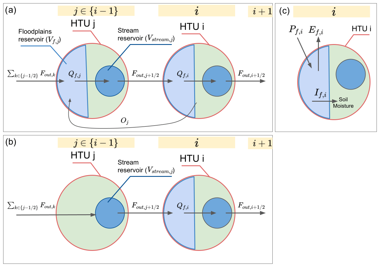
Figure 1Scheme resuming the movement between the different reservoirs for an HTU which has floodplains and its upstream HTUs if (a) the upstream HTU has floodplains or if (b) the upstream HTU does not have floodplains, as well as (c) the fluxes between the HTU, the atmosphere and the soil moisture.
The volume of water in the stream reservoir of an HTU i (Vstream,i) follows the water continuity equations in Eq. (5), differentiating whether it is an HTU with or without floodplains.
with
-
Fout,j with the water flowing from the stream reservoir of the upstream HTUs to the HTU i
-
the outflow from the stream reservoir of HTU i into the stream reservoir of the downstream HTU i+1
-
Qf,i the water flowing from the floodplain reservoir of the HTU i to the stream reservoir of the HTU i (this variable will be explained in the following subsection).
The outflow from the stream reservoir is also affected by the presence of floodplains through a reduction factor based on the fraction of the HTU. The more the HTU is flooded, the more the flow out of the stream reservoir is reduced. This factor aims to represent the impact of the floodplains on the reduction in the river discharge. The floodplain reservoir has its own time constant; therefore, this factor is exclusively used for the stream reservoir. Due to the HTUs structure, some small HTUs over the main river can have a flooded fraction close to 1 that impedes the river from flowing, and a parameter Rlimit, equal for all HTUs, has been implemented to limit this flow reduction. This parameter is the same for all the HTUs. The reduction factor can be deactivated with a value of Rlimit=0. Therefore, the formulation of the outflow from the stream reservoir of an HTU i which has floodplains () differs from Eq. (4) and is represented in Eq. (6).
The flooded fraction fi used in Eq. (6) is calculated from the area of the HTU which is flooded (Sf,i). This value is diagnosed using Eq. (7).
The appropriate function Γ will be discussed further in Sect. 2.4.
2.3.2 Floodplain reservoir
This subsection focuses on the definition of the different water fluxes related to the floodplain reservoir. The water continuity equation governing the temporal changes in the volume of water in the floodplain reservoir (Vf,i) is presented in Eq. (8). The different components of this equation will be described further in this subsection.
with
-
Fout,j with the water inflow into the floodplains from the upstream HTUs
-
Oj with the overflow of HTU i into the floodplain reservoir of the upstream HTUs
-
the overflow of HTU i into the floodplain reservoir of the upstream HTUs
-
Pf,i the rainfall onto the floodplain
-
Ef,i the evaporation from the flooded surface
-
If,i the infiltration from the floodplain into the soil moisture reservoir.
Within an HTU i with floodplains, the flow of water from the floodplain reservoir to the stream reservoir (Qf,i) has the same type of formulation as Eq. (4). This formulation is presented in Eq. (9).
The floodplain scheme allows a specific HTU to “overflow” the content of its floodplain reservoir into connected upstream HTUs with floodplains. This process is driven by the difference in height between the elevation of the water and that of the neighbouring HTUs:
with
-
z the elevation at the outflow of the HTU
-
h the water level in the floodplains.
As long as , there is no overflow (). When the water rises over the elevations of the upstream HTU, the overflow is enabled. The flux is proposed to be
with “OF” the time constant of the overflow (in days).
At the edge of the atmospheric grid cell, some small HTUs are created due to the overlap between the catchments and the grid cells. These HTUs may generate numerical issues such as unrealistically high Δh values due to their small area. The volume of water which overflows from an HTU to its upstream HTU is calculated from the excessive floodplain height Δh and a surface. In order to solve the undesirable numerical effects, both the surface of the HTU which overflows and that of its upstream HTU are considered using the following surface: the term .
Excessively low values of the OF time constant are another source of numerical instabilities (the lower the OF, the more important the overflow). For example, if the HTU i overflows in various upstream HTUs, an excessive transfer of water at once will leave a negative volume in the floodplain reservoir which generates an oscillation between HTU outflow and downstream overflow. It is a time step issue which depends on the choice of OF relative to the time step of the scheme. It is possible to increase the overflow without generating instabilities by using a time-splitting scheme to solve this, i.e. by repeating the overflow operation several times during the same time step using a slower time constant OF. The number of repetitions of the overflow water transfer within a single time step is defined by the parameter OFrepeat.
2.4 Floodplain geometry
Another crucial aspect of the floodplain scheme is the relationship between the volume of water in the floodplain reservoir (Vf,i), the surface of open water and the water surface elevation of the floodplain. In order to establish a simple but meaningful relationship, some assumptions about the geometry of the floodplains are necessary.
As the HTUs are constructed from higher-resolution hydrological data, it is possible to derive a direct relationship using the topography data from the hydrological pixels (Dadson et al., 2010; Zhou et al., 2021; Fleischmann et al., 2021; Chaney et al., 2021). But this method would bring two different issues: (1) the uncertainty about the topography over lowlands such as floodplains and (2) the high computational memory cost. The memory cost involved may not necessarily be worth the improvement it would bring to the simulation.
For this reason, the definition of the floodplain shape has been simplified by using two variables controlling the shape of the floodplains, such as that proposed by D'Orgeval (2006) and shown in Fig. S2a in the Supplement. These variables are the following:
-
h0,i is the height at which the floodplains of the HTU reach their full extension, i.e. .
-
βi is the shape of the floodplain which will control how quickly it fills. βi>1 corresponds to a floodplain with a concave cross-section (as Fig. S2b), whereas βi<1 corresponds to a floodplain with a convex cross-section. βi=1 represents a triangular cross-section.
In D'Orgeval (2006), both variables have been set to constant values: β=2 and h0=2 m. With the high-resolution floodplain scheme, it is possible to define β and h0 more precisely using the characteristics of the HDEM pixels combined within an HTU. This is described in Sect. 2.4.3.
The spatial representation of the floodplains in an HTU i is defined by the relationship between the volume of water in the floodplains Vf,i, the surface of the floodplains Sf,i and the water surface elevation of the floodplain hi. It is considered that at a certain height h0, the whole floodplain is flooded, i.e. Sf=Sfmax and that, even if the floodplain height is higher than h0, the flooded area cannot exceed this limit (see Eq. 12). The shape of the floodplains will have an influence only for hi<h0 because above h0, the height is considered to increase linearly with the volume.
2.4.1 Cases of floodplains not fully flooding
If we consider an HTU i which has a potential flooded area of 100 %, i.e. with or , the relationship between the flooded area Sf,i and the height of the floodplain hi for hi<h0 is represented in Eq. (13).
This assumes that the transect of the floodplain has an exponential shape, and with the choice of β it can be decided how quickly it fills. The relation between the floodplain height and the volume in the floodplain reservoir is obtained by integrating this function between 0 and hi, yielding
This provides the Γ function introduced above to calculate the surface from the volume. The above equations are only valid for .
2.4.2 Cases of fully flooded floodplains
If , we have . Equation (15) shows the relationship between the flooded surface and the volume in the floodplain reservoir by combining Eqs. (13) and (14).
In order to generalise, the floodplain height above h0 increases linearly with the volume. Defining Vfmax,i as the volume at which , when , the flooded surface and the floodplain height in the HTU follow respectively Eqs. (16) and (17).
2.4.3 Orography and shape of the floodplains
The elevation is a variable available for each pixel in the HDEM. Considering an HTU i, the reference elevation is defined by the elevation of the outflow pixel (zi), while h0,i is the lowest difference in elevation between zi and its upstream HTUs reference elevation (see Eq. 18).
The β variable has been estimated using the standard deviation of the distribution of the elevation, including the values for all the HDEM pixels within the HTU. The different values of standard deviation are bounded by lowlim_std=0.05 m and uplim_std=20 m and are then converted to obtain the β variable which ranges between values of lowlim_beta=0.5 and uplim_beta=2.
With the hypothesis that h0,i is the height at which the floodplain of the HTU i is totally flooded, this height is assumed to be the minimum of the difference between elevation of the HTU i and the ensemble of its inflows that have floodplains ({i−1}). When hi is larger than this difference, it means that the floodplain of i will be able to overflow to the upstream vertices.
The conversion of water volume in the floodplain reservoir into an open-water area has been assessed by testing different values of the default parameters defining the floodplain shape (β and h0). Its result is that, although these parameters can lead to important changes over a single HTU, they have a limited influence on the total flooded area over a larger region (not shown).
2.5 Ancillary data
2.5.1 ORCHIDEE's high-resolution routing
The routing in ORCHIDEE has been constructed by the routing pre-processor (RoutingPP) presented in Polcher et al. (2023). It allows for combining different high-resolution hydrological information to construct the HTUs and calculate their characteristics. In this case, the routing graphs have been constructed using the MERIT-Hydro dataset at a 2 km resolution.
2.5.2 Spatial description of the floodplains
The Global Lakes and Wetlands Database (GLWD; WWF, 2004) available at a 1 km resolution has been interpolated to the HDEM used to define a mask of potentially flooded areas based on the following categories: (1) freshwater marsh, floodplains; (2) reservoir; and (3) pan, brackish saline wetland. Therefore, the floodplain mask is available for each pixel of the hydrological data. These data allow for calculating a potentially flooded area for each HTU during the routing construction.
The floodplains in GLWD cover all of the Pantanal region. Before using the floodplain scheme over other large floodplains, it is necessary to assess the relevance of the spatial extent of the categories considered floodplains in GLWD. In the case of the inadequacy of the GLWD representation over the region, other datasets can be used to define the potentially flooded area.
There is a large uncertainty in the description of wetlands due to the difficulty of perfectly evaluating the flooded areas from satellite products, and there are also large uncertainties concerning the categorisation. Despite this uncertainty, GLWD is combining different types of products to obtain this categorisation. The review of other wetland descriptions in Hu et al. (2017) does not seem to show a product that would be preferable to GLWD. In this study, the GLWD dataset has not been modified, but the categories in the GLWD dataset related to floodplains may be further changed in other studies to adjust the floodplain mask.
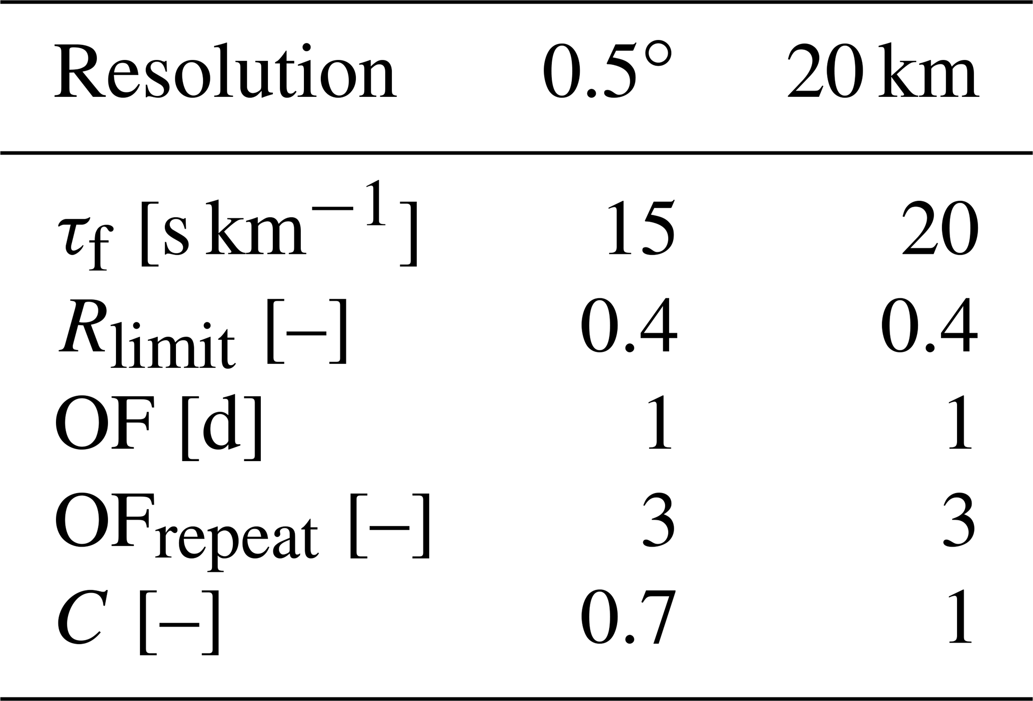
2.5.3 Calibration of the parameters
The different parameters of the floodplain scheme have been calibrated based on the simulated discharge at the Porto Murtinho station, which is the reference station at the outflow of the Pantanal (Brazil; lat 21.7∘ S, long 57.9∘ W), between 1991 and 1996 in comparison to the observations considering (1) the variation in the discharge through its correlation with the observations and (2) the mean value and variability in the discharge. The choice of the 6-year calibration period was due to a limited number of available years from the simulations (24 years). Therefore, the model has been calibrated over this reduced period common to both forcings so that the analysed results are not influenced by an overfitting effect. Considering that our model has a reduced number of physical variables, we consider it is not necessary to assess it on large periods as we assumed that these parameters are relatively independent of the hydrological cycle variability. However, we agree that performing the calibration over a larger period could have been preferable, but we faced two limitations concerning this point: (1) the period of the simulations (AmSud was only available from 1990 to 2019) and (2) a technical limit due to the resources (time and computational resources) needed to run the simulations.
The parameter with the largest influence on the variability in the discharge is τf, the time constant of the floodplain reservoir. This parameter has an important impact on the annual cycle of the discharge at Porto Murtinho station. The [αstream,αfast] interval is considered a valid interval for τf. This interval has been discretised to select different possible values for τf. It has been assessed along with Rlimit, which is the second parameter with the largest influence on the discharge. For Rlimit, we discretised the [0,1] interval to obtain possible values. In a first step, these two parameters were calibrated together, and we performed a grid-search evaluation, which means that we evaluated all the existing combinations of possible discretised values over the intervals for τf and τf to select the combination with the best performance to represent the observed discharge.
In a second step, we assessed the parameters related to the overflow, which have a limited impact on the discharge OF and OFrepeat. These parameters slightly influence the temporality of the discharge. In this case, we also assessed these two parameters using a grid-search evaluation considering a discretisation of the following intervals: [0.5, 2 d] for OF and [one repetition, five repetitions] for OFrepeat.
Finally, the last parameter to calibrate is the infiltration constant (C) which determines the loss to soil moisture and, thus, potentially to evaporation. This parameter with a very reduced impact on the discharge only reduces or increases the level of the discharge at the outflow of the region. We discretised the [0,1] interval to assess it.
The values of the parameters found depended on the resolution of the atmospheric forcing and are shown in Table 1. The parameterisation for the 0.5∘ resolution has been established with WFDEI_GPCC atmospheric data forcing and for the 20 km resolution with AmSud_GPCC atmospheric data forcing, which are both described in more detail in the following section. It is recommended to make a sensitivity test before using the scheme over another region to evaluate if this parameterisation is the more appropriate.
Table 1parameterisation of the floodplain scheme depending on the resolution of the atmospheric grid.
3.1 Methodology of validation and analysis
Two pairs of ORCHIDEE simulations using the high-resolution routing (HR) are used to perform the validation of the floodplain scheme and the analysis of the impact of the floodplains on ORCHIDEE. Each pair is forced by a different atmospheric forcings – WFDEI_GPCC at 0.5∘ resolution and AmSud_GPCC at 20 km resolution – and is composed of a simulation with the floodplain scheme activated (FP) and another one without the floodplain scheme (NOFP). The use of two forcings with different resolutions allows us to assess the influence of the resolution and the forcing uncertainty of the floodplain scheme. The forcings are further described in Sect. 3.3.
The analysis is performed between 1990 and 2013, which is the period over which both forcing datasets are available. The following validation and analysis of the simulation will focus on the mean values and annual cycle of the variables between 1990 and 2013 but will also consider their mean values over different seasons during this period: the flood season from March to May (MAM) and the dry season from September to November (SON).
3.2 Model description: ORCHIDEE
The simulations presented in this publication are the output of offline ORCHIDEE simulations, i.e. simulations of the ORCHIDEE LSM forced by an external atmospheric dataset containing the atmospheric data required to run the model (downward longwave and shortwave radiations, precipitation, 2 m air temperature, wind speed, 2 m specific humidity, snowfall, and rainfall).
Ancillary datasets provide information about vegetation cover and the soil composition.
The soil properties are described by the combination of the three main soil textures: coarse, medium and fine from the USDA soil description (Reynolds et al., 2000).
The vegetation in ORCHIDEE is described in the model's input by the potential vegetation cover (maxvegetfrac) for 12 different plant function types (PFTs) and the fraction of bare-soil cover. This bare soil can be covered by different types of non-vegetated land surfaces such as glaciers, cities, lakes or flooded areas. For each grid cell, the sum of the maxvegetfrac of the different PFTs and the bare-soil surfaces is equal to 1. In these simulations, the PFTs are constructed from the ESA-CCI database (European Space Agency Climate Change Initiative; ESA, 2017). Readers should be aware that the original ESA-CCI remote PFT classification has been post-processed to the 13 ones used in ORCHIDEE.
The vegetation cover is defined by the fraction of the grid cell occupied by each PFT (vegetfrac) whose upper limit is maxvegetfrac. It is driven by the leaf area index (LAI, in m2 m−2) of the PFT; if LAI ≥ 1, then vegetfrac equals maxvegetfrac, and elsewhere the fraction not covered by this vegetation type is considered by the model as bare soil.
The potential vegetation cover used in these simulations is shown in Fig. S3. It shows maxvegetfrac over the region for the different PFT categories existing over the Pantanal. There is a high presence of tropical broadleaf evergreen on the western and northeastern part of the Pantanal covering more than 50 % of the grid cells in this region. The tropical broadleaf raingreen is present over all the Pantanal with a cover of around 20 % of each grid cell. The rest of the Pantanal is mainly covered by natural grassland of C3 (in the northwest, the south and the east) and C4 type (in the north and the south–southeast).
The hydrology in ORCHIDEE is represented through an 11-layer soil scheme (de Rosnay et al., 2000, 2002; Campoy et al., 2013) representing the vertical movement of the water in the soil and the transfer of heat.
The surface energy budget is the partitioning of the total net radiation composed of the net longwave and shortwave radiations () into latent heat fluxes (LE), sensible heat fluxes (H) and ground heat fluxes (G); see Eq. (21). The net shortwave radiation is determined by the albedo (α) at the surface because , with SWin the incoming shortwave radiation. In the model, the impact of the flooded area on the albedo is not considered, but the changes in soil moisture and vegetation directly affect this parameter and, therefore, impact the net radiation.
The latent heat flux is represented by the latent heat of vaporisation (L) and evapotranspiration (E). The sensible heat fluxes (H) in the ORCHIDEE LSM are driven by the difference between the surface temperature (Ts) and the temperature of the air at the surface (Ta). It is calculated from Eq. (22) with cp the specific heat.
Over a large period, the ground heat fluxes can be neglected, and then Rn is only partitioned into LE and H (G=0). Thus, the relative distribution of LE and H is important to quantify the changes in the surface energy budget and the temperature changes. This can be expressed with the evaporative fraction (EF), which is the ratio of latent heat (LE) over the total land–atmosphere fluxes, i.e. the sum of the latent heat and the sensible heat (LE +H):
The EF index indicates the distribution of the heat fluxes over land. The value of this index tends to 0 when there are no latent heat fluxes, such as in arid areas. It can take the value of 1 if there are only latent fluxes and take values over 1 when the land surface is cooled because in this case H<0.
3.3 Forcings
WFDEI_GPCC is a 0.5∘ resolution atmospheric forcing dataset for land surface models (Weedon et al., 2014). It is derived from the ERA-Interim re-analysis processed by the WATCH Forcing Data methodology (Dee et al., 2011) and has a temporal resolution of 3 h and a spatial discretisation of 0.5∘. WFDEI_GPCC corresponds to the version of WFDEI whose precipitation has been bias-corrected by the GPCC dataset (Schneider et al., 2017).
AmSud_GPCC is a 20 km resolution forcing based on the bias-corrected AmSud simulation, a 30-year simulation performed with the RegIPSL regional model (Guion et al., 2022) from 1990 to 2019 and using ERA5 re-analysis data for the boundary conditions. The precipitation of the AmSud simulation has been bias-corrected by the GPCC monthly precipitation, adjusting the monthly precipitation total by a multiplicative factor for each grid cell to obtain the AmSud_GPCC forcing. This has been done to correct the negative biases of precipitation over the southern Amazon and northern La Plata Basin (i.e. the Upper Paraguay River Basin).
It must be emphasised that neither of these two forcings includes the impact of the floodplains and, thus, includes large biases in lower atmospheric temperature and humidity over this region.
As ORCHIDEE is used in offline mode, the atmospheric conditions are fixed and the floodplain parameterisation does not interact with the atmosphere and does not affect the atmospheric conditions. Therefore, these forcings will be a source of errors for the near-surface temperature and humidity because they will not respond to the changes related to the presence of flooded areas in the model.
It should also be noticed that, compared to WFDEI_GPCC, AmSud_GPCC has a higher evaporative demand due to overestimated near-surface temperature and incoming shortwave radiation and an underestimation of near-surface humidity (see Fig. S4). This is partly related to the fact that the AmSud_GPCC forcing is only bias-corrected for the precipitation; the other variables remain unchanged. Therefore, as the precipitation is underestimated over the region in AmSud, the other variables represent a drier atmosphere over the Pantanal.
3.4 Discharge
The National Hydrometeorological Network managed by the Brazilian National Water Agency (Agência Nacional de Águas – ANA) has provided the monthly river discharge observations for the Porto Murtinho station.
This station is considered the reference outflow for the Pantanal (Schrapffer et al., 2020; Penatti et al., 2015). Moreover, its large continuous data record allows for choosing the period of simulation freely to evaluate the floodplain scheme.
3.5 Flooded area
Depending on the period simulated, the simulated flooded area was assessed by different estimates of the flooded area over the Pantanal.
The evolution of the flooded area over the 20th century has been estimated by Hamilton et al. (1996) and Hamilton (2002), extrapolating the correlation between river height and the flooded area established over the period 1979 and 1987.
Padovani (2010) performed a satellite estimate of the flooded area by applying a linear spectral mixture model to MODIS data between 2002 and 2009.
Apart from Hamilton (2002) and Padovani (2010), the satellite estimate of the flooded area based on the modified normalised difference water index (mNDWI) using the normalised difference between green and shortwave infrared bands presented in Schrapffer et al. (2023a) is also used to assess the flooded area in the FP simulations.
The Global Inundation Extent from Multi-Satellites version 2 (GIEMS-2; Prigent et al., 2020) database is a satellite estimate of flooded areas (agricultural irrigation and wetlands) which is principally constructed using passive microwave observations but also using visible and near-infrared reflectance data from optical satellites. GIEMS-2 is a global monthly dataset available at a 0.25∘ resolution between 1992 and 2015. As for GIEMS version 1, GIEMS-2 is largely used to validate the floodplain representation in different models (Zhou et al., 2021; Marthews et al., 2022).
We use different types of satellite products to have a complete view on the flooded area. Two products have been specially constructed over the Pantanal – Hamilton (2002) and Padovani (2010) – so they may be more appropriate due to the specificity of the Pantanal floodplains. However, they have some limitations: Hamilton (2002) is based on a relationship between flooded area and river height established during a short and wet period, and, therefore, this relationship may differ under different climatic conditions. It is also only available up to 2000. Concerning Padovani (2010) and Schrapffer et al. (2023a), the limitation is the infrequent revisit of satellite (data every 6 d) and missing images due to the use of optical satellite imagery. Padovani (2010) is interpolated, which helps us to have an overview of the complete time series of flooded areas, while Schrapffer et al. (2023a) gives us precise estimates for precise dates without any interpolations and is available up to 2013, while Padovani (2010) is only available up to 2010. Therefore, both datasets are complementary. GIEMS-2 is a global dataset and a reference in the scientific literature in terms of satellite estimates of the flooded area, but it has not been specifically validated over the Pantanal; however, we thought it was crucial to include it here.
3.6 Water mass
In ORCHIDEE total water storage (TWS) is defined by summing the different reservoirs of the routing scheme (slow, fast, stream and floodplains) and the soil moisture to obtain an estimate comparable to the water storage from the Gravity Recovery And Climate Experiment (GRACE) satellite (Ngo-Duc et al., 2007).
The GRACE (Schmidt et al., 2008) satellite mission is a USA–German collaboration, launched in March 2002. The GRACE twin satellite aims to estimate the changes in the mass redistribution near the surface which are related to different processes by evaluating the changes in the gravity fields. GRACE data represent the anomaly of water mass normalised by the values obtained during the 2004–2010 period. The data from GRACE are available from 2002 onwards.
In order to reduce the signal-to-noise ratio, it is recommended to use the GRACE data at a spatial scale of 90 000 km2 (Vishwakarma et al., 2021). The extension of the Pantanal of approximately 150 000 km2 (Barbosa da Silva et al., 2020) is large enough to be able to use GRACE. Although the area is large enough to justify the use of GRACE, there can be an error related to the overlap of pixels. Still, GRACE is the best tool available at this moment to perform this type of analysis. Also, the comparison with GRACE is more of a qualitative than a quantitative one.
4.1 Discharge
The annual cycle of the discharge between 1990 and 2013 is shown in Fig. 2. The activation of the floodplain scheme improves the seasonality of the annual cycle with a peak in July in the FP simulations as in the observations instead of February as in the NOFP simulations. The mean annual discharge and the amplitude of the discharge are also reduced in the FP simulations compared to NOFP and are therefore in better agreement with observations. This can directly be explained by the loss of water from the river system to the soil moisture (floodplain infiltration) and the direct evaporation from the floodplain. However, the amplitude of discharge simulated in FP is still overestimated, with higher discharge during the peak and lower discharge between November and February. This discharge is more important in WFDEI_GPCC_FP than AmSud_GPCC_FP.
The main mechanism behind the river discharge delay is that the water is delayed in the floodplain reservoir. Another part of the delay is also related to the infiltration of the water in the floodplains into the soil, which faces a larger delay. Then, evapotranspiration also plays an important role as it will reduce the mean annual river discharge.
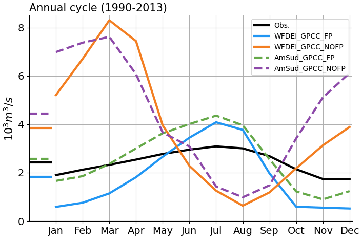
Figure 2Annual cycle of the discharge at the Porto Murtinho station between 1990 and 2013 for the simulations with (blue) and without (orange) the floodplain scheme activated for the forcings WFDEI_GPCC (solid line) and AmSud_GPCC (dashed line) compared to the observations (black line). The mean annual discharge is represented by a horizontal line on the left.
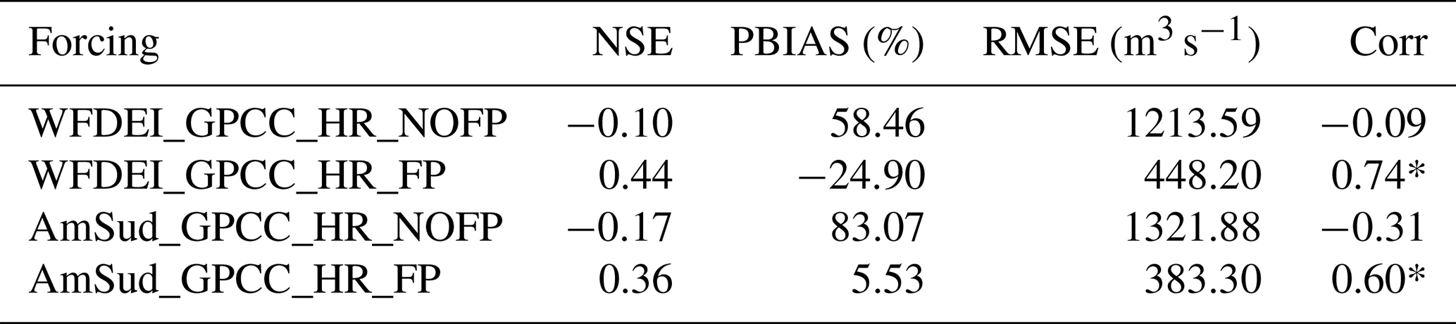
The statistical indexes calculated to summarise the analysis based on the monthly discharge are presented in Table 2 and are described in Sect. S1 in the Supplement. The activation of the floodplain scheme leads to a substantial improvement in the simulations with higher values of the correlation and the Nash–Sutcliffe model efficiency coefficient (NSE), while the root mean square error (RMSE) is closer to 0 and the percent bias (PBIAS) is lower. The correlations with observations of the simulated discharge in the NOFP simulations are not significant. WFDEI_GPCC_FP has a better correlation and NSE than AmSud_GPCC_FP, while the opposite is true for the PBIAS and the RMSE. Based on the previous analysis, WFDEI_GPCC_FP seems to better represent the annual cycle of discharge compared to AmSud_GPCC_FP, which results in higher correlation and NSE, but, as the amplitude of the annual cycle is higher than in the observations, its RMSE and PBIAS are worse than the values for AmSud_GPCC_FP.
Considering the dry atmospheric bias and thus higher potential evaporation in AmSud_GPCC compared to WFDEI_GPCC and the fact that both forcings have similar precipitation, we may expect the discharge in AmSud_GPCC_FP to be lower than the discharge in WFDEI_GPCC_FP; however, the opposite is true. This suggests that the resolution of the interactions with the atmosphere may be playing a role in the representation of the floodplain processes and, therefore, in the water cycle of the basin. For the same floodplain scheme, the coarser resolution has difficulties representing the low flows, and it results in a strong overestimation of the difference between the high and low values of discharge compared to the observations. The simulations without floodplains (WFDEI_GPCC_NOFP and AmSud_GPCC_NOFP) have similar low flows and variability. From Polcher et al. (2023), we know that an increased number of HTUs does not change the simulation of the discharge. Therefore, we can conclude that the effect of the floodplains on the hydrology seems to be better captured by the high-resolution simulation.
Table 2Evaluation of the discharge at the outflow of the Pantanal for the simulations with the high-resolution routing scheme both with and without the floodplain scheme activated forced by two atmospheric forcings with a different resolution (WFDEI_GPCC and AmSud_GPCC) using statistical indexes (NSE, PBIAS, RMSE, Corr). The asterisk signals that the correlation has a level of significance higher than 99 %.
The inter-annual variability has also been assessed and is shown in Fig. S5. The FP simulations with floodplains have higher correlations with observations compared to the NOFP simulations concerning the inter-annual variability in the mean annual discharge. However, these correlations are only significant for WFDEI_GPCC simulations. Also, this correlation is much higher in WFDEI_GPCC_FP (correlation of 0.71) compared to AmSud_GPCC_FP (correlation of 0.17). Figure S6b shows the de-seasonalised time series of the monthly discharge at Porto Murtinho. We can observe that the FP simulations are less noisy and much closer to the observations compared to the NOFP simulations. The inter-annual variability in the monthly discharge at Porto Murtinho is shown in Fig. S8. We can observe that the floodplain scheme reduces the variability in the discharge. Between October and April, the variability in the FP simulations is close to the observed discharge variability. From May to September, the variability in the monthly discharge is overestimated compared to the observation. This overestimation is higher in WFDEI_GPCC_FP compared to AmSud_GPCC_FP.
4.2 Water mass
The water mass in the WFDEI_GPCC and AmSud_GPCC pairs of simulations is analysed in this subsection to help understand the dynamics of the model in its representation of the water cycle at different resolutions.
The evolution of the monthly total water mass anomaly in the simulations normalised by the 2004–2010 mean values can be compared to GRACE over the Pantanal region. Due to its resolution, GRACE is a coarse estimate, but it can provide a general overview and qualitative evaluation of the representation of the water cycle in the model. Therefore, the area considered for calculating the anomaly of the normalised total water storage for GRACE and the simulation is a rectangle that goes from 61 to 53∘ W and from 15 to 21∘ S. It includes the Pantanal, which represents a third of the total area over this rectangle.
Table 3 shows the correlation between the total water mass anomaly from GRACE and the simulations. The high level of correlation shows that all the simulations show an annual evolution similar to that observed by GRACE. However, the small differences between the FP and the NOFP simulations for both forcings have to be noted. This means that the model is properly representing the evolution of the water volume in the reservoirs over the Pantanal but that the floodplain reservoirs have little impact on the total water storage.
Table 3Correlation between the anomaly of total water storage from GRACE and the volume of water in the different reservoirs over the Pantanal region between 2003 and 2013 normalised by the mean and standard values between 2004 and 2010. The asterisk signals that the correlation has a level of significance higher than 99 %.
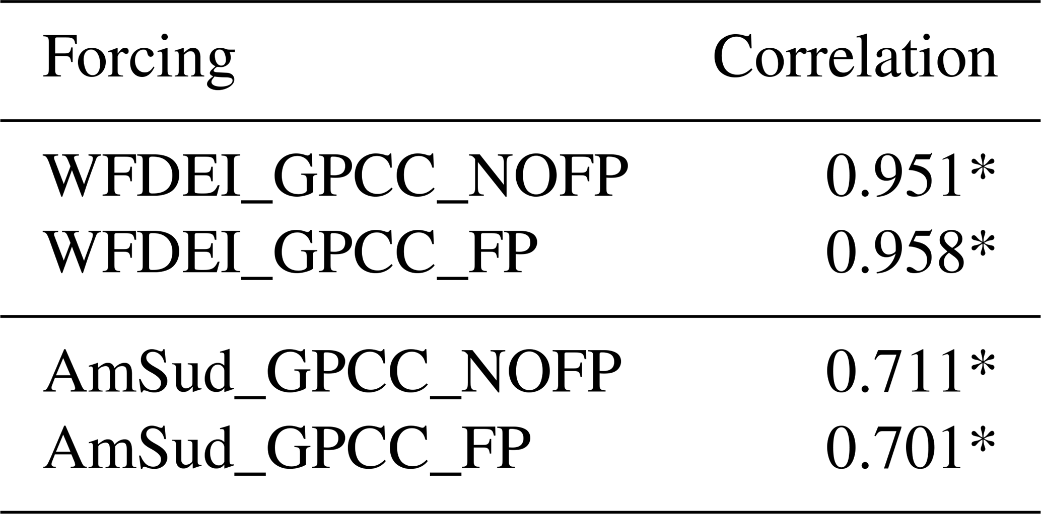
Figure 3a compares the contribution of different reservoirs in the model over the Pantanal through the annual mean of the water volume within each one of them. The floodplain scheme has a similar impact on the reservoirs at both resolutions. The volume of water in the soil moisture and the stream reservoir increases significantly when activating the floodplain scheme. The relative increase is more important in the fast and slow reservoirs, even if in absolute value it represents a smaller increase compared to the stream and soil moisture reservoirs. The activation of the floodplains allows for storing more water in the river network when the floodplain scheme is activated.
The annual cycle of the water volume within the different reservoirs of the model over the Pantanal is shown in Fig. 3b–f. The soil moisture over the Pantanal is the largest contribution to the total water storage, followed by the stream reservoir and the floodplain reservoir in the FP simulations. The activation of the floodplains increases soil moisture due to the infiltration of the water from the floodplain reservoir but does not significantly impact its temporal evolution (see Fig. 3b). This explains why the floodplain scheme does not have an impact on the correlation of the total water storage over the Pantanal. Concerning the stream reservoir (see Fig. 3c), we observe a change that is similar to the change in the discharge at the Porto Murtinho station because this is the reservoir that drives the discharge. The floodplain reservoir (see Fig. 3d) logically has a value of 0 in the NOFP simulation and follows the evolution of the stream reservoir in the FP simulations because these reservoirs are connected. The content of water in the slow reservoir (see Fig. 3e) plays, in the model, the role of the aquifers. Its volume strongly increases due to the floodplains, and this is related to increased deep drainage induced by the higher soil moisture infiltration when the floodplains are activated (see Fig. 3b). The water content in the fast reservoir (see Fig. 3f) displays much lower volumes compared to the other reservoirs. However, it is higher in the FP simulation compared to the NOFP simulation. This can be explained by the increase in runoff in the FP simulations compared to the NOFP simulations (not shown). This increase is much higher in WFDEI_GPCC than in AmSud_GPCC.
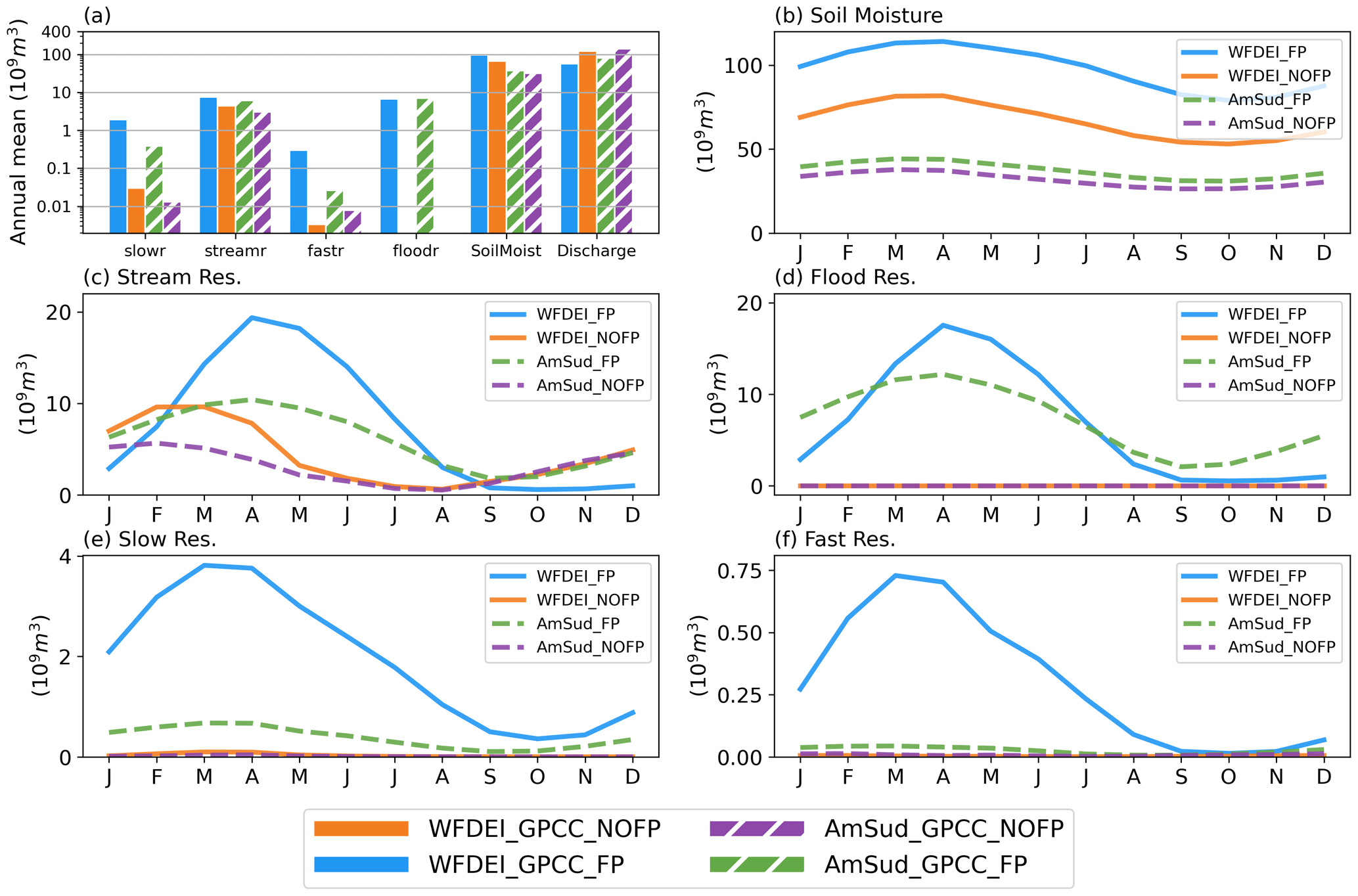
Figure 3Annual mean of the column of water in the different reservoirs over the Pantanal region (a) and annual cycle of the content of water in the different reservoirs over the Pantanal region: soil moisture (b), stream (c), flood (d), slow (e) and fast (f) for the pair of simulations FP and NOFP forced by WFDEI_GPCC and AmSud_GPCC. A logarithmic scale is used to facilitate the comparison.
The water volumes are higher in WFDEI_GPCC for the fast, slow and stream reservoirs compared to AmSud_GPCC. This can be related to the higher evapotranspiration in AmSud_GPCC compared to WFDEI_GPCC due to the dry bias in the atmospheric conditions in this forcing. The higher evapotranspiration decreases soil moisture, drainage and runoff. In consequence, the volume in the fast and slow reservoirs also decreases. The stream and flood reservoirs are less affected by the higher evapotranspiration over the Pantanal as their dynamic is more influenced by the water from the upstream areas that flow into the Pantanal. The origin of the overestimated annual variability in discharge at Porto Murtinho in WFDEI_GPCC_FP can be attributed to the slow, fast, stream and floodplain reservoirs which have a more pronounced amplitude of their annual cycle than AmSud_GPCC, with a much higher volume of water in the slow and fast reservoirs.
In conclusion, the floodplains involve relatively small masses of water compared to the total water storage over the region, but these volumes are of great importance as they directly affect the river discharge and form open-water surfaces which will impact the land–atmosphere interaction.
4.3 Flooded area
The evolution of the simulated flooded area for the FP simulations is presented in Fig. 4. In this case, the flooded area is compared to the observational-based estimates over the period 1992–2013 as it allows for a direct comparison with different satellite-derived products: GIEMS-2 (Prigent et al., 2020), Hamilton (2002) and Padovani (2010). The flooded area in WFDEI_GPCC_FP is higher than in AmSud_GPCC in terms of mean value and inter-annual variability. Despite the differences, the mean value of the flooded area is within a similar range of value in both simulations with the floodplains activated.
There are discrepancies between different satellite estimates considered in this study. Hamilton (2002) tends to estimate higher areas compared to GIEMS-2, while the opposite is true for Padovani (2010) and the mNDWI-based satellite estimate from Schrapffer et al. (2023a). The mean value of the simulated extent seems to be underestimated by the model compared to satellite estimates and corresponds to the lowest value of the satellite estimate. The annual variations are correlated, but the variability in the simulated flooded area is strongly underestimated.
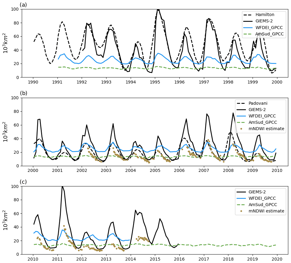
Figure 4Time series of the flooded area in the simulations with the high-resolution floodplain scheme (HR) forced by WFDEI_GPCC and AmSud_GPCC for the 1990s (a), 2000s (b) and 2010s (c) in comparison to the different satellite estimates available over the region: Hamilton (2002) until 2000, Padovani (2010) between 2000 and 2010, GIEMS-2 (Prigent et al., 2020) for the period 1992–2015, and the flood estimate based on MODIS MOD09A1 using the mNDWI spectral index (Schrapffer et al., 2023a).
GIEMS-2 also allows us to directly compare the observed spatial extent with the simulated area in ORCHIDEE. Figure 5 represents the geographic distribution of the flooded fraction averaged over the 1992–2013 period, as well as the temporal correlation and root mean square error between each simulation and GIEMS-2. The structure of the mean flooded fraction in AmSud_GPCC_FP and WFDEI_GPCC_FP is similar to GIEMS-2 (cf. northern region and floods over the main Paraguay river). The flooded area at the centre of the Pantanal is not captured by the model; this is related to the presence of the Taquari megafan, which is an area of divergent flows that is very sensitive to the orography and cannot be represented in this model (Louzada et al., 2020; Assine, 2005) because the model's river network is convergent and only assumes a downstream flow. Both forcings result in a similar structure of the flooded areas, and the simulation using the higher-resolution forcing captures the spatial pattern better. The higher resolution in AmSud_GPCC_FP allows for observing the higher concentration of flooded area over the main Paraguay river and the impact of the overflow to the adjacent grid cell. At higher resolution, the overflow is more important as the HTUs are smaller and, therefore, reach higher floodplain heights over the largest river.
The correlation between time series of flooded areas over the Pantanal in the simulations and GIEMS-2 (Fig. 5c and g) is relatively high in the northern and central regions, reaching values higher than 0.6. However, the flooded fraction south of the Pantanal has no correlation in the AmSud_GPCC_FP. This may be related to the presence of ponds which are isolated from the flood pulse of the large rivers flowing through the Pantanal (Nhecolândia ponds; Guerreiro et al., 2019).
The differences between the simulations and GIEMS-2 are also assessed grid point by grid point using the root mean square error over the region in Fig. 5d and h. Lower values show a good correspondence of the flooded fraction between the model and GIEMS-2, while the higher values (darker grid points) show larger discrepancies. The major error are related to (1) the Taquari megafan flooded area not represented in the model; (2) the flooded areas in the northeast (Cuiabá and São Lourenço rivers) which are not present in GIEMS-2; and (3) the fact that the flooded areas in AmSud_GPCC are concentrated along the main rivers, while the flooded areas are more extended in GIEMS-2.
Although the variability in the floodplains seems to be underestimated in the model, the spatial representation of the flooded area is realistic. The high-resolution atmospheric grid allows a more precise description of the flooded area. The underestimation of the variability can be related to (1) the fact that the model handles separately the saturated soils and the flooded area, while the satellite estimates consider them together; (2) the conversion of the volume of water in the floodplain reservoir into a flooded area whether it is related to low sensitivity of the conversion formulation or the volume of water considered for the conversion; and (3) the lack of lateral expansion of the floodplains into the grid cells adjacent to the main river which, although it is partly covered by the overflow from the floodplains, may be underestimated due to some missing processes such as the groundwater lateral flow.
Concerning the first point, the satellite estimate of the flooded area may erroneously consider saturated soils as a water surface (Zhou et al., 2021; Aires et al., 2018). Therefore, the satellite-based estimates of floodplain extent could cover open-water surfaces, surfaces with a high soil moisture content and flooded vegetation. The model, on the other hand, considers separately soil moisture and open-water surface in the floodplains and renders the floodplain extent difficult to compare. In GIEMS-2, the floods in the eastern region of the Pantanal appear to be more important during the wet season (DJF) compared to the flood season (MAM), while other studies show that this region is not regularly flooded (Padovani, 2010). There is a high correlation between GIEMS-2 flooded fraction and the soil moisture down to 0.5 m depth from the surface in the NOFP simulation (see Fig. S7), which confirms the hypothesis of a saturated soil moisture signal in the GIEMS-2 dataset related to the precipitation during the rainy season. This saturated soil moisture is directly handled in the model by the soil hydrology and does not appear as a flooded area.
Finally, the major cause of the underestimation of the flooded area is related to the limited lateral expansion of the floodplains. The floodplain scheme only considers the overbank flow, and this limitation shows that some processes need to be integrated into the model. For instance, the exchange between surface water and groundwater can raise the water table, therefore driving large-scale groundwater transports which are not foreseen by ORCHIDEE's routing scheme at a scale larger than the HTU (slow and fast reservoirs) and its corresponding grid cell. These processes are particularly important in the complex hydrology of the Pantanal region (Junk and Wantzen, 2004; Freitas et al., 2019).
An implicit lateral transfer of moisture is carried out within the vadose zone through the soil moisture scheme (de Rosnay et al., 2000, 2002; Campoy et al., 2013). As water in the floodplain infiltrates, it will affect the soil moisture of the entire atmospheric grid cell and, thus, modify its exchanges with the atmosphere. This effect will be enhanced at lower resolution because the grid cells have larger areas, and, therefore, the increase in soil moisture related to the floodplain infiltration will affect more important areas. Therefore, there is a numerical diffusion at the resolution of the atmospheric grid which helps but has no physical cause. The soil hydrology is managed with a 1-D vertical model and, therefore, does not integrate the possibility of transferring laterally the increased soil moisture of the floodplains to the neighbour grid cells.
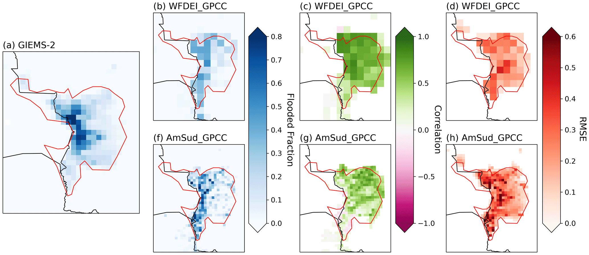
Figure 5Mean flooded fraction in GIEMS-2 (a), WFDEI_GPCC (b) and AmSud_GPCC (f). Evaluation of the spatial representation of the floodplains in ORCHIDEE using the correlation (c, g) and the root mean square error (d, h) for WFDEI_GPCC (c, d) and AmSud_GPCC (g, h) compared to GIEMS-2.
4.4 Other floodplains
It is difficult to evaluate the floodplain scheme on other South American floodplains because the flooding process in other large wetlands in South America is not always mainly driven by overflow from large rivers, as is the case for the Pantanal. Some other types of wetlands can exist and have a major influence over the flooded area, such as the swamps and flooded forests over in the Llanos de Moxos, in the Bananal and in the surroundings of the Amazon River (see Fig. S9). Another difficulty is that there are not always observations available to assess the impact of the activation of the floodplain scheme on the basin hydrological cycle (absence of hydrological stations or stations without data).
Nevertheless, analysis has also been performed over the Llanos del Orinoco despite the absence of observations at the station at the outflow of the floodplains using both simulations between 1990 and 2013 (see Figs. S10 and S11). This flood mechanism is driven by overflow from large rivers (floodplains), but there is also an important area in which the flood mechanism is related to swamps and flooded forest processes in the south, north and east (see Fig. S9).
The discharge at the outflow of the Llanos del Orinoco is delayed by 1 month, and the flooded area is underestimated due to the absence of the integration of swamps and flooded forests. We can also observe the absence of coastal floodplains which are related to other floods mechanisms. As shown in Fig. S9, the Inner Niger Delta is a region that has been adapted to evaluate the floodplain scheme that is also mainly composed of the “freshwater marsh, floodplain” category in GLWD.
5.1 Soil moisture
The presence of the floodplains induces an additional infiltration into the soil. Figure 6 shows the mean soil moisture for the FP simulations and the relative difference with the NOFP simulations averaged between 1990 and 2013 considering the period of maximum flooding (March, April, May), the dry period (September, October, November) and the entire year. The soil moisture is considered down to 0.5 m below the surface because our main interest is the upper layers of the soil which are the most affected by the floodplain infiltration.
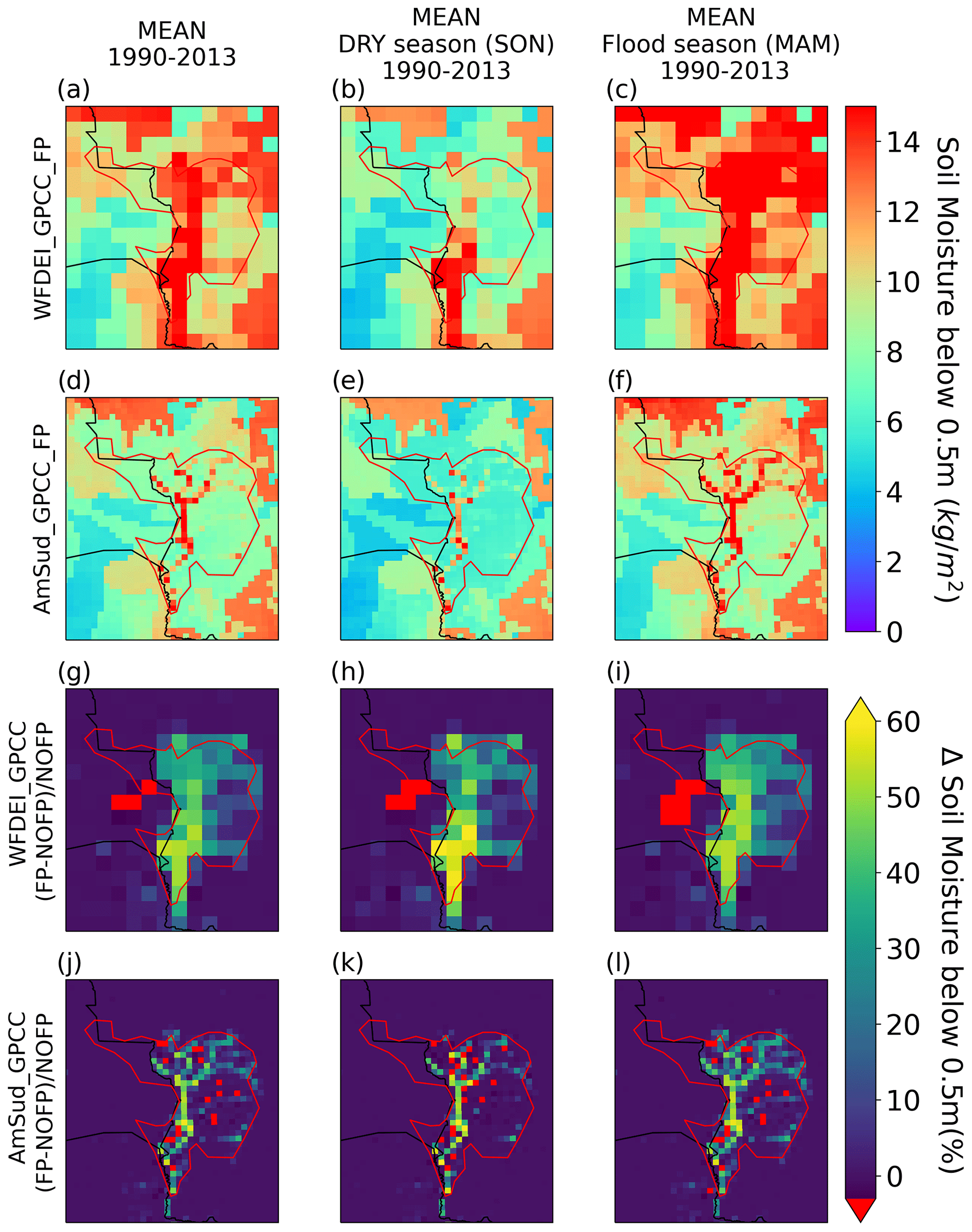
Figure 6Mean soil moisture over the upper level (down to 0.5 m below the surface) during the 1990–2013 period considering the full year (a, d, g, j), the dry season (SON; b, e, h, k) and the flood season (MAM; c, f, i, l) for the WFDEI_GPCC_FP simulation (a, b, c) and the AmSud_GPCC_FP (d, e, f). Difference between the FP and NOFP simulations for WFDEI_GPCC (g, h, i) and AmSud_GPCC (j, k, l).
The soil moisture increases over the most flooded area, and it reflects the structure of the hydrological network in the Pantanal. The comparison with the NOFP simulation shows that these changes occur over a larger area during the flooded season compared to the rest of the year. The relative differences between the FP and the NOFP simulations reach the highest values during the dry season because of the larger contrast with the dry conditions when no floodplains are considered.
The impact of floodplains on soil moisture is more important at lower-resolution forcing because of the implicit numerical diffusion occurring at the level of the atmospheric grid. This compensates for the missing processes related to the shallow aquifers in the model. The groundwater flows and other missing riparian processes are quite complex, but they can have an important impact on the soil moisture conditions (Krause et al., 2007; Frappart et al., 2011; Girard et al., 2003).
The introduction of the floodplains has also led to the reduction in soil moisture in some grid cells close to the largest rivers in the region. The soil moisture decreases over some grid cells that are near the large rivers in the AmSud_GPCC_FP simulations compared to AmSud_GPCC_NOFP. In this case, soil moisture receives water from the floodplains through infiltration, while the floodplains collect part of the precipitation that would have gone directly into soil moisture elsewhere. If the infiltration from the floodplains supplying soil moisture does not compensate for the decrease in direct precipitation received, the soil moisture may decrease. This occurs in the north and central eastern Pantanal over grid points with a low volume of water in the floodplain reservoir because no important rivers are flowing through the grid cell. In this case, the infiltration from the floodplains can be smaller than the amount of precipitation going into the floodplain reservoir instead of directly increasing soil moisture. This phenomenon is enhanced in regions with low infiltration rates (lower infiltration coefficient; see klitt).
5.2 Vegetation
The state of the vegetation is presented through the leaf area (LAI) variable, which determines within ORCHIDEE also the fraction of vegetation in the grid cell. Soil moisture, through plant transpiration and carbon assimilation, is one of the main drivers of vegetation and its LAI. This is why vegetation is also affected by the floodplain scheme.
Figure 7 shows, for each vegetation type existing in the Pantanal in ORCHIDEE, the ratio of the vegetation cover to the maximum surface it can occupy during the flood season (no hatch) and the dry season (hatched) for the FP and NOFP simulations in blue and orange respectively for the WFDEI_GPCC (Fig. 7a) and the AmSud_GPCC simulations (Fig. 7b). It should be noted that both simulations have the same vegetation description input. Although the LAI drives this process, we consider here the ratio as it allows for evaluating the development of the vegetation relative to the maximal vegetation cover it reaches for LAI>1 m2 m−2.
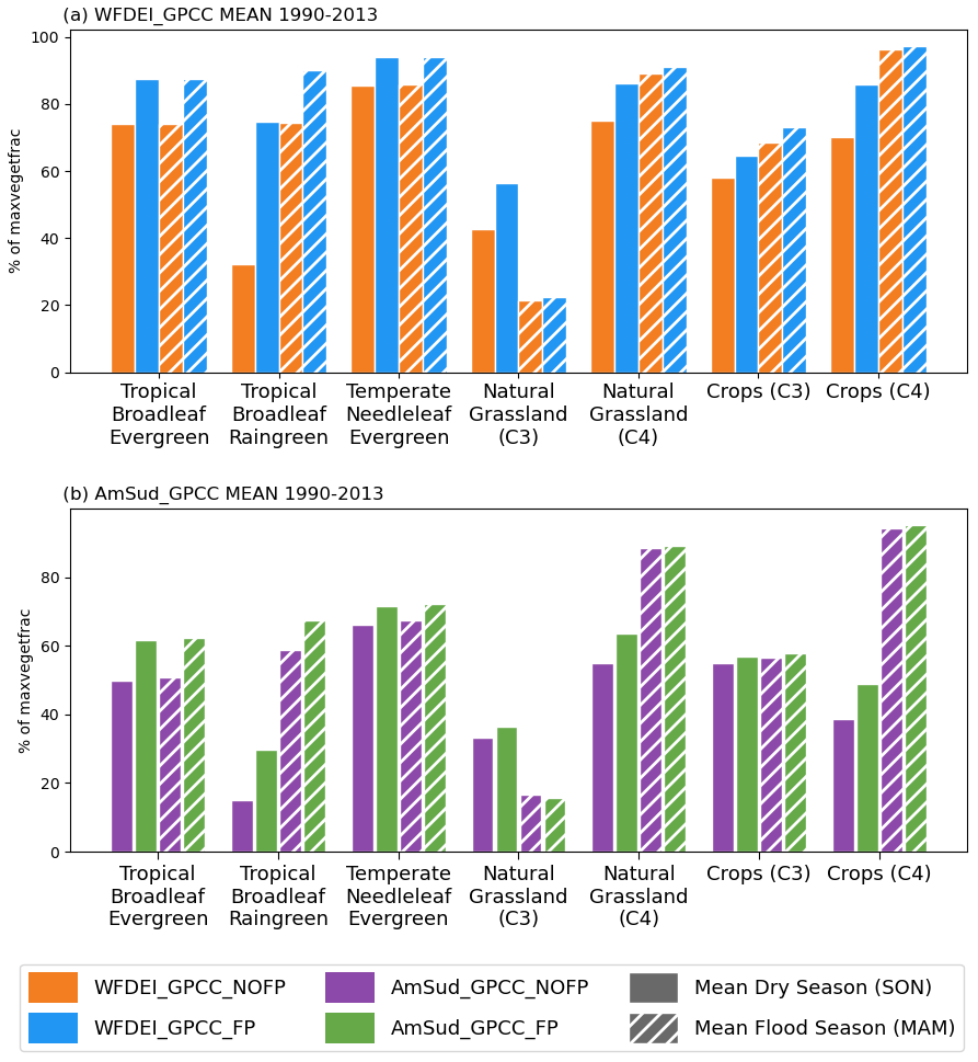
Figure 7Bar plot of the percentage of the maximum vegetation cover in the model for the FP (blue) and NOFP (orange) simulations during the dry season (SON; no hatch) and during the flood season (MAM; hatched) for the simulations forced by WFDEI_GPCC (a) and AmSud_GPCC (b).
All vegetation types are affected by the floodplains except for C3 crops in AmSud_GPCC. For most of these PFTs, the difference only occurs during the dry season such as for natural C3 and C4 grasses and C4 crops. For tropical broadleaf (evergreen and raingreen) and temperate needleleaf evergreen, this change occurs during both the flooded and dry seasons. For short vegetation, the floodplains mainly enhance vegetation fraction during the dry seasons as they have shallow roots and thus only have access to upper-soil moisture. For tall vegetation, on the other hand, the increased vegetation fraction is more persistent as roots can exploit the increased deep soil moisture.
Some regions of the Pantanal see their vegetation fraction decrease with the activation of the floodplain scheme. This can be explained by the reduction in the soil moisture related to the floodplains explained previously and observed in Fig. 6.
The ratios of surface occupied by the PFT to its maximum are generally higher in the simulations forced by WFDEI_GPCC, which is related to the larger increase in soil moisture (see Fig. 6). The changes between the FP and NOFP simulations are also higher for WFDEI_GPCC compared to AmSud_GPCC, which is related to the larger impact of the floodplains on soil moisture in WFDEI_GPCC. These results show that ORCHIDEE without floodplains is unable to develop the vegetation detected by ESA-CCI and thus has a systematic bias in this region. Only activating the floodplain allows the development of the vegetation that is observed. Therefore, the floodplain scheme is important for a more realistic simulation of the vegetation over these regions. This occurs, for example, to the tropical broadleaf raingreen, which is particularly affected by the floodplain scheme. This vegetation type has an important presence in the north of the Pantanal (see Fig. S3). Without floodplains, this vegetation type does not have enough soil moisture to grow correctly and cover the observed maximum area in the model.
As a qualitative assessment, the average simulated LAI over the Pantanal is compared to the Global Inventory Modeling and Mapping Studies-3rd Generation V1.2 (GIMMS-3G+) data for the normalised difference vegetation index (NDVI) (Pinzon et al., 2023) in Fig. S15. The LAI time series have significant correlations with the NDVI time series, but the NOFP simulations have a higher correlation compared to FP simulations. This seems to be caused by the delayed peak of LAI in the FP simulation.
The higher development of the vegetation in FP (driven by higher LAI values) also increases the roughness height for momentum and heat in the ORCHIDEE model (not shown). These variables have an impact on the turbulent exchange coefficients in the calculation of latent and sensible heat within ORCHIDEE. Once coupled, this impact will propagate to the planetary boundary layer and also affect the momentum transport in the lower atmosphere.
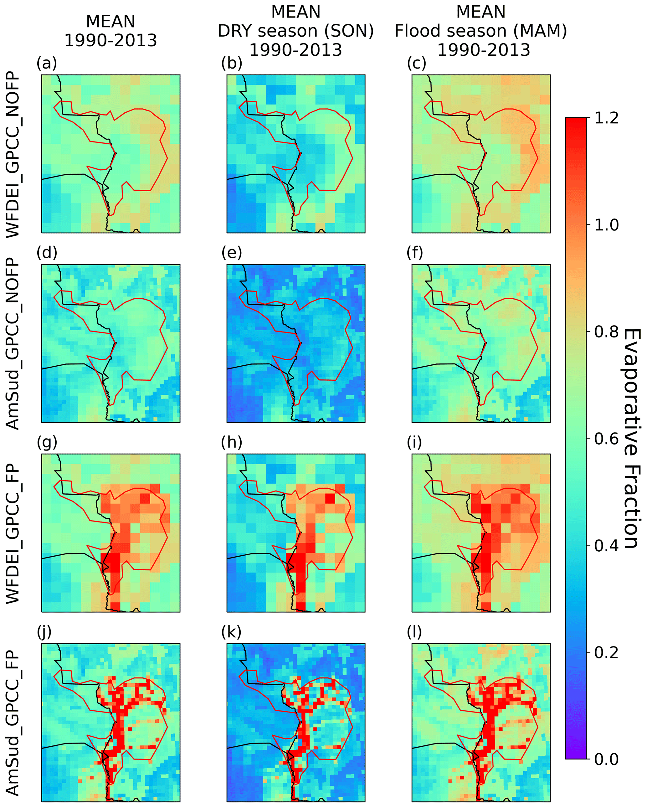
Figure 8Mean evaporative fraction for each grid cell in WFDEI_GPCC_NOFP (a–c), AmSud_GPCC_NOFP (d–f), the WFDEI_GPCC_FP (g–i) and the AmSud_GPCC_FP (j–l) for the period 1990–2013 considering the full year (a, d, g, j), the dry season (SON: b, e, h, k) and the flood season (MAM; c, f, i, l).
5.3 Surface energy budget
As seen in Sect. 3.2, over a large period (such as decades) net radiation can be partitioned between the latent and sensible heat flux. To compare the relative distribution of energy in latent and sensible heat flux, the evaporative fraction is shown in Fig. 8 for the NOFP simulations and the FP simulations.
The evaporative fraction increases throughout the Pantanal region, which means that the surface energy budget shifts towards energy lost to water-phase changes. The latent heat fluxes increase while the sensible heat fluxes decrease. The largest differences follow the spatial structure of the flooded area.
In both simulations, the highest values of mean evaporative fraction exceed 1, which is accentuated in the AmSud_GPCC_FP simulation. This means that over the main floodplains, the sensible heat fluxes become negative for some grid cells, which indicates a surface cooler than the atmosphere over the large period – i.e. on a 24-year average in this case (see Eq. 22). This behaviour is probably unrealistic in a tropical region and is related to the absence of feedback from the atmosphere. In this offline set-up of ORCHIDEE evaporative demand is high because air temperature and humidity have been established (in the re-analysis for WFDEI and the atmospheric model for AmSud_GPCC) without considering the floodplains. The lower-atmospheric conditions thus become incoherent from the simulated surface conditions when the floodplains are activated. This also explains the higher values in AmSud_GPCC_FP compared to WFDEI_GPCC_FP due to the higher evaporative demand in this forcing. It shows that the changes brought about by floodplains are so fundamental in the surface energy balance that they cannot be considered without the coupling to the atmosphere.
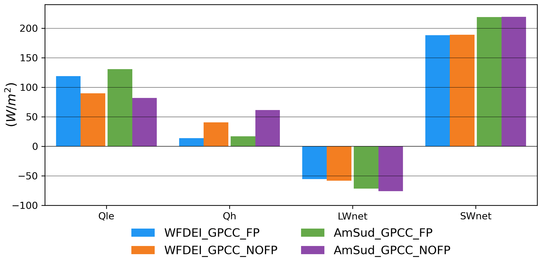
Figure 9Average value over the Pantanal of the different terms of Eq. (21) () between 1990 and 2013.
Figure 9 evaluates the averaged terms of the surface heat budget. The ground heat fluxes are not shown as they are negligible compared to the other fluxes. In Eq. (21), the sensible and latent heat fluxes are not the only variables that can be changed by the floodplains. Net surface radiation is also impacted by albedo changes induced by stronger vegetation development when floodplains are activated.
In general, albedo decreases when the soil moisture increases and when the vegetation density increases. However, albedo may also vary depending on vegetation types and soil types (clay, sand, silt). The vegetation cover increase will impact the albedo differently for different vegetation types. The vegetation type can have a higher albedo than the local bare soil; therefore, the albedo may increase when this vegetation type develops over regions with scarce vegetation, replacing a low-albedo bare-soil cover. The net shortwave radiation (SWnet) in the NOFP simulations has values close to the FP simulations. It is, as expected by the analysis of the forcings, higher in AmSud_GPCC. This means that although the albedo slightly changes with the floodplain scheme, it does not have an important impact on the surface energy budget. The net longwave radiation (LWnet) slightly increases in the FP simulation compared to the NOFP, induced by the decreased surface temperature.
The latent (Qle) and sensible (Qh) fluxes have more important changes between the NOFP and the FP simulations. The latent heat flux increases in the FP simulation compared to the NOFP by 30 % (WFDEI_GPCC) and 60 % (AmSud_GPCC), while the sensible heat flux decreases by 70 % in both forcings.
Therefore, the changes in surface temperature and energy balance find their principal origin in the impact of the floodplains on the latent and sensible fluxes instead of the changes in net radiation.
5.4 Evapotranspiration
The changes in the surface energy budget are dominated by modifications of the water available for evapotranspiration and enhanced by the development of vegetation. These impacts are reflected in the annual cycle of the different components of evaporation (bare soil, transpiration, floodplain evaporation and interception loss), which are shown for both atmospheric forcings in Fig. 10.
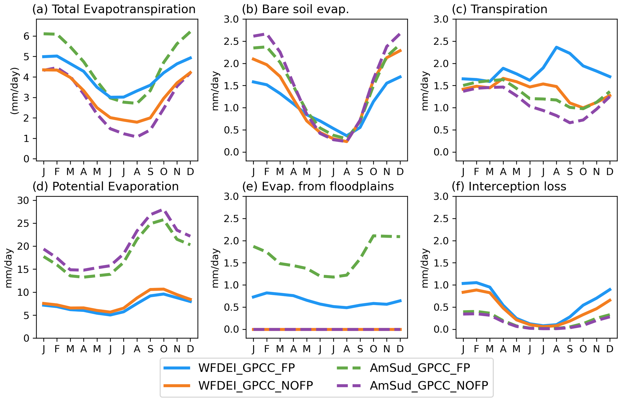
Figure 10Annual cycle of the evapotranspiration variables for WFDEI_GPCC (solid lines) and AmSud_GPCC (dashed lines) for the simulation with (blue) and without floodplains (red): (a) total evapotranspiration, (b) bare-soil evaporation, (c) transpiration, (d) potential evaporation, (e) evaporation from floodplains and (f) interception loss.
Potential evaporation is lower throughout the year in the FP simulations when compared to NOFP. This is a direct consequence of the decrease in surface temperature over the floodplains which will decrease the saturated surface humidity, and the lack of adjustment of the lower atmosphere which should be more humid than assumed in the forcing datasets. This is confirmed by the fact that the potential evaporation changes between NOFP and FP follow the same spatial structure as the surface temperature (not shown). Despite this decrease in the potential evaporation, the actual flux is higher in the FP simulations with the largest increases occurring between June and October, which corresponds to the drier part of the year. This is a consequence of the fact that evaporation over the area of the floodplains is water-limited when the lateral flows are not taken into account. It is only when water is allowed to converge in the floodplains that a sufficient amount of water becomes available to support evapotranspiration despite lower potential evaporation in FP. The floodplain evaporation brings the total flux to levels closer to those estimated in Schrapffer et al. (2020) through a water balance estimation using observations and numerical simulations. This leads us to believe that evaporation is more realistic when the floodplain scheme is activated.
Bare-soil evaporation is similar in both simulations, although it is slightly higher in the NOFP simulation during the wet season. Bare-soil evaporation is limited by the precipitation over bare soil and not affected by the lateral transport of water. The amount of precipitation over bare soil is reduced in the simulation with floodplains because of the reduced bare-soil area due to the increased vegetation fraction for most of the PFTs, inducing a decrease in the rainfall over bare soil as the precipitation falling over the flooded fraction of the grid cells directly goes to the floodplain reservoir of the HTUs of the grid cell.
Transpiration is higher in the FP simulation between June and November. It is the largest change apart from direct open-water evaporation. This change is explained by (1) the increase in the LAI and the vegetation fraction (vegetfrac) in the FP simulation and (2) the increased soil moisture available to support plant photosynthesis during the drier part of the year. Comparing the transpiration between WFDEI_GPCC_FP and AmSud_GPCC_FP, there are higher values in WFDEI_GPCC_FP during the dry season. This difference is consistent with the impact on soil moisture described above and is another consequence of the observed numerical diffusion issue.
The interception loss is higher in the FP simulation compared to the NOFP simulation during the rainy season since the canopy in the FP simulation can intercept more water due to the higher LAI and the higher vegetation cover.
The other main difference is that the evaporation from the floodplains is much higher in AmSud_GPCC (around 1.5–2 mm d−1) compared to WFDEI_GPCC (around 0.4–0.5 mm d−1) which is related to the higher flooded area in AmSud_GPCC and the higher incoming radiation in AmSud_GPCC when compared to WFDEI_GPCC.
The differences in evapotranspiration between FP and NOFP simulations have also been assessed spatially (not shown). They follow the spatial patterns of changes in evaporative fraction (see Fig. 8). These changes in evaporative fraction are driven by both the increase in soil moisture and the presence of open water in the simulations with the floodplain scheme activated. In WFDEI_GPCC, these changes are mainly driven by the soil moisture changes, while in AmSud_GPCC, they are dominated by the higher fraction of flooded areas due to the numerical diffusion effect discussed above. Both resolutions respond differently to the floodplain scheme, which explains the need for different parameter values at each resolution.
Ideally, the floodplain scheme should behave the same way at all resolutions. However, the crude assumptions imposed by the definition of soil moisture at the atmospheric grid level and not the HTU scale explain most of the differences. It thus seems important in these regions of important horizontal surface moisture convergence to link soil moisture to the hydrological rather than the atmospheric grid of a land surface model. The use of a specific sub-surface component such as suggested in the framework for LSM described in Hallouin et al. (2022) can be used to solve these issues by providing a tridirectional movement of the water in the ground with a lateral movement driven by topographic and hydraulic head gradients.
The resolution of the forcing has an impact on the relative importance of the different floodplain processes, such as the balance between soil moisture and flooded area. However, the impact of the floodplains on the evapotranspiration and the land–atmosphere fluxes is similar at all resolutions. Moreover, it should be added that there is a lack of observations over the region, which complicates the development of the parameterisation of this type of model.
5.5 Temperature
Surface temperature (Ts) is determined by the surface energy balance at the surface and will thus be directly affected by the impact of floodplains on evaporation.
The Pantanal is in a tropical region that receives large radiation fluxes throughout the year. Therefore, when floodplains are not considered, the underestimation of water brought by the convergence of rivers in the floodplains leads to an underestimation of evaporative cooling and, therefore, an overestimated surface temperature.
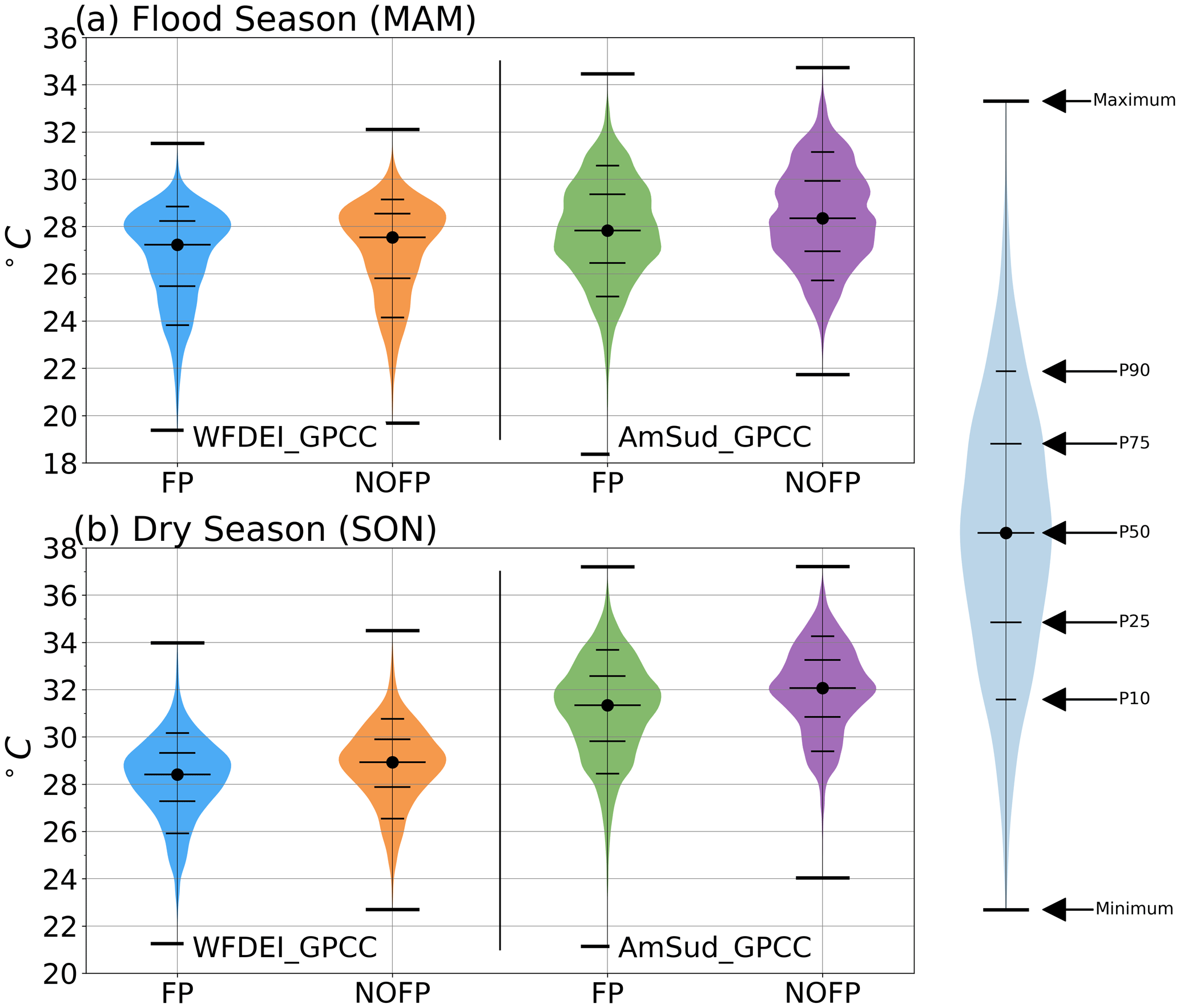
Figure 11Representation of the distribution of the average daily temperature over the most flooded part of the Pantanal for the pair of simulations with (left) and without floodplains (right) forced by WFDEI_GPCC and AmSud_GPCC during the period 1990–2013. The extrema; the media; and the percentiles 10, 25, 75 and 90 are represented.
Due to its dry bias, AmSud_GPCC atmospheric forcing has a higher near-surface temperature and specific humidity than WFDEI_GPCC. This explains the higher surface temperature in AmSud_GPCC_NOFP compared to WFDEI_GPCC_NOFP.
The activation of the floodplain scheme reduces surface temperature over the Pantanal (see Fig. S12), driven by the increase in evaporation described previously. The difference in temperature is lower for the WFDEI_GPCC forcing (around −1 ∘C) compared to AmSud_GPCC (with differences up to −3 ∘C during the flood season and up to −6 ∘C during the dry season).
Observational temperature datasets such as CRU TS4 (Harris et al., 2020) do not reflect any hydrological pattern of temperature difference over the Pantanal (cf. Figs. S13 and S14). This is due to the scarcity of in situ observations over the region and the coarse resolution of observational datasets which interpolate these in situ observations.
The distribution of the average daily temperature over the most flooded parts of the Pantanal (with a mean flood_frac>0.1) in both forcings is shown in Fig. 11. During the flood season (MAM, Fig. 11a), the activation of floodplains reduces both maximum and minimum values for AmSud_GPCC and WFDEI_GPCC. In both cases, the body of the distribution (the distribution between percentile 10 and 90) is shifted toward lower temperature and is more concentrated, as can be seen by the change in the shape of the distribution of values.
During the dry season (Fig. 11b), the body of distribution of the temperature, as well as the extremes, is shifted toward lower values. The reduction in minimum temperature is more important in AmSud_GPCC, whose minimum is 3∘ lower than the minimum of AmSud_GPCC_NOFP in both seasons.
In conclusion, the increased evapotranspiration dampens temperature extremes caused by meteorological and radiation fluctuations.
With the progress made in the description of surface flows in land surface models and especially with increasing resolutions, the parameterisation of the interactions of these flows with the landscape needs to be revised. In this article, we proposed a methodology to implement the representation at higher resolution of the floodplains in a land surface model and, as a first benchmark, evaluate its performance over the Pantanal region in South America, performing offline simulations (forced by atmospheric forcings) at different resolutions. Figure 12 summarises the impacts of the presence of floodplains on the land surface variables in ORCHIDEE.
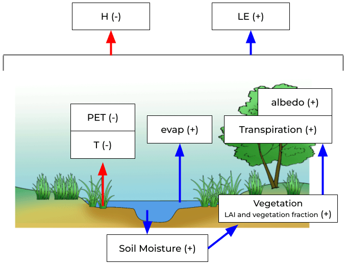
Figure 12Summary of the different impacts of the floodplains over the land surface variables in a land surface model.
Offline simulations were performed to validate and analyse the functioning of the floodplain scheme. A pair of experiments for each atmospheric forcing has been performed, one with (FP) and another one without floodplains (NOFP), and allows for exploring the role of atmospheric forcing uncertainty and resolution on our ability to reproduce the impact of floodplains on surface–atmosphere exchanges. The pair of simulations has been forced by atmospheric conditions with different resolutions and different atmospheric water demands but the same precipitation. These forcings underestimate the near-surface humidity and temperature because they did not consider the impact of the floodplains on the atmosphere and because these regions have scarce in situ observations; however, the 20 km forcing has a higher atmospheric evaporative demand due to its lower near-surface humidity and higher near-surface air temperature and incoming radiation.
The floodplain scheme presented in this article exploits the high-resolution information of the hydrologically coherent digital elevation model used to construct the HTUs. This allows us to describe the shape of the floodplains with more precision. The resolution of the hydrological units increases compared to the previous version of the floodplain scheme (D'Orgeval, 2006). The exploitation of the high-resolution river graph allows for improving the description of the floodplains within the hydrological units and to parameterise the overbank flow of the HTUs. The infiltration of the floodplains into the soil is a crucial aspect as it permits the floodplains to affect a larger area. However, the soil moisture in ORCHIDEE is still managed on the atmospheric grid level and, therefore, creates an uncontrolled numerical diffusion which will have to be addressed in the future. This new version of the floodplain scheme integrates the possibility for the water in the floodplains to overflow in the floodplains of the upstream HTUs, which was not possible in the previous version and is crucial at higher resolution. The calibration of the parameters could be avoided if we can define them based on physical relationships. However, this is not always possible because the calibration of these parameters can hide some missing processes, such as is the case with the floodplain infiltration adjusted as the complex vegetation and soil of the floodplains (flooded vegetation and soil covered by sediments).
The representation of the water cycle over the Pantanal has been assessed by comparing the discharge simulated at the station of Porto Murtinho, which is at the outflow of the Pantanal. In both cases, the activation of the floodplain scheme improves the simulation of the discharge at the outflow of the Pantanal by shifting the peak flows and reducing the amplitude. Still, the intra-annual variability in discharge is overestimated for both forcings but less so in the higher-resolution version. The water mass in the floodplains has only a limited impact on the total water storage and, thus, could not be validated with GRACE data. Although the floodplains represent a relatively small volume of water, they have an important impact on river discharge and surface–atmosphere interactions.
The mean flooded area is coherent between both AmSud_GPCC_FP and WFDEI_GPCC_FP simulations, and the annual cycle is underestimated for both forcings compared to different satellite estimates. However, there are epistemological difficulties in defining “flooded area” and large discrepancies between the various satellite estimates considered here. It is difficult to correctly assess the flooded area (Schrapffer et al., 2023a) principally covered by vegetation and over-saturated soils and, therefore, to correctly identify the deficiencies of the model. The representation of the flooded area is a major issue for any flooding scheme. Under the assumption that the precipitation from the GPCC dataset is correct over the Pantanal and knowing that the river discharge is close to the observation when the floodplain scheme is activated, it can be concluded that the water cycle of the catchment is correctly represented in the model. Therefore, the issues can come from (1) the fact that there exist different ways to define what a flooded area is (Schrapffer et al., 2023a), (2) the conversion of the volume of water in the floodplains to flooded area and (3) missing processes such as groundwater transfers. The estimate of flooded areas can take different forms such as the presence of shallow water or flooded vegetation and can be related to some groundwater resurgence. The satellite products consider the open-water surfaces and the regions with high soil moisture content, while they are considered separately in the model. In the model, the flooded area is modelled through the relationships between the volume and water surface elevation of the floodplain and the flooded area. More complex methods could be considered if elevation were known to have a higher accuracy in these flat areas. Yet, it should be remembered that there are still large uncertainties in the DEM over flat regions and even more if there is an important vegetation cover (Yamazaki et al., 2019). Several tests have been performed to evaluate the sensitivity of the predicted flooded area from the water volume in the floodplain reservoir. These tests have shown that this volume–area function does not seem to play an important role at a large scale in the estimated total flooded area over the region. ORCHIDEE uses a convergent flow model; however, in some cases, the floodplains can be caused by a divergent flow such as the Taquari megafan over the Taquari river in the central region of the Pantanal. The representation of this type of process would require a high-precision hydrological DEM as the floodplains in this region are very sensitive to small differences in orography. The divergent processes are not represented in the hydrological DEM and, therefore, are not implemented in ORCHIDEE. However, some models such as MGB-IPH and CaMa-Flood represent this divergent process by analysing high-resolution topography data (Pontes et al., 2017; Yamazaki et al., 2014). The groundwater fluxes between grid cells are not considered either in the actual versions of ORCHIDEE. The water that infiltrates from the floodplain reservoir of an HTU affects only local soil moisture and is not transported in the saturated layers of the ground. However, this increase in the soil moisture should be able to affect the neighbouring grid cells (Krause et al., 2007; Frappart et al., 2011; Girard et al., 2003). These small-scale processes are implicitly integrated for coarse atmospheric resolutions, such as the 0.5∘ grid used here. However, at higher resolution, these processes need to be represented explicitly.
The soil moisture would be better represented if it was calculated at the resolution of the river graph, i.e. at the HTU level. However, this will aggravate the lack of the uncontrolled numerical diffusion currently occurring and thus call for a physical representation of the horizontal diffusion in the saturated soil layers. To do so, the hydro-geological structures within the Pantanal would need to be clarified and used in the representation of the horizontal diffusion.
The vegetation dynamic is strongly affected by flooding and the soil moisture increase. The infiltration of water from the floodplains into the soil increases vegetation density even during the dry season. These have impacts on ORCHIDEE's other surface properties, such as the roughness height for momentum and the roughness height for heat. The albedo decreases over almost all the Pantanal but increases over the most flooded part due to the covering of the dark soil by a vegetation type with a higher albedo. The maximal potential vegetation cover in ORCHIDEE for a vegetation type is constructed from satellite-derived products, but these vegetation types require a realistic water availability to grow to their full potential in the model. Without floodplains, some PFTs derived from satellites do not thrive. The improved coherence between the potential vegetation cover and the development of the vegetation in the model is a good indicator of the fact that the floodplain scheme improves the land surface simulations over the Pantanal.
Land–atmosphere fluxes over the Pantanal are also affected by the activation of the floodplain scheme with the sensible heat fluxes diminishing, while the latent heat fluxes are increasing. This is coherent with the surface temperature decrease over the floodplains. The changes between the FP and NOFP simulations showed that the net radiation change is low compared to the sensible and latent heat fluxes; thus, the balance between the two fluxes is the main change in the surface energy budget.
The model allows us to observe the different origins of the changes in the latent heat fluxes. The principal contribution to the increase in evapotranspiration is transpiration followed by open-water evaporation. Transpiration also plays an important role, a consequence of the increase in soil moisture and vegetation density. However, its impact is more limited over the Pantanal at higher resolution due to the ill-controlled numerical diffusion of soil moisture and the lack of horizontal moisture diffusion in the saturated layers of the soil. The potential evaporation is lower in the FP simulation due to the decrease in surface temperature but does not affect the actual flux as the increased water availability dominates.
The absence of coupling leads to high and unrealistic values of evaporative fraction showing that it is possible that the latent heat fluxes may be overestimated and the evapotranspiration too. This has been observed more clearly in the forcing AmSud_GPCC which represents an atmosphere with a higher evaporative demand compared to WFDEI_GPCC. The AmSud_GPCC and WFDEI_GPCC are issued from AmSud and ERA-Interim, both of which do not include floodplains. The near-surface observations available in the regions and used to bias correct the re-analysis are insufficient to compensate for this lack of information in the model. The forcings do not integrate the impact of the floodplains on near-atmosphere conditions and are not reacting to the surface conditions. Thus, despite the higher evapotranspiration the near-surface humidity remains low and enhances, more than it should be, the evapotranspiration. The coupling between ORCHIDEE and an atmospheric model will help in analysing the impact of the floodplains under more realistic conditions (with feedback from the atmosphere) and give the opportunity to better analyse the land–atmosphere interactions.
Over the Pantanal, the floodplain scheme seems to capture the dominant hydrological processes involved, but, looking at the subject with a wider angle, other types of processes could be critical in regions we refer to as floodplains. For example, the open-water surfaces can also be related to some ponds or lakes and to different types of flooded forests or swamps. The configuration proposed here is not optimal for these other types of wetlands. Some other schemes can be constructed from the spatial description of these processes and their interaction with the atmosphere, such as for ponds, which are small lakes flooded due to the local precipitation, or swamps and flooded forest, which can be managed by redirecting small fractions of river flow into soil moisture in areas of long residence times. Spatial descriptions of wetlands are needed to discriminate between all the different types of flooded areas, which have different dynamics and must be parameterised differently from the floodplain scheme described in this paper.
To conclude, the different impacts of the floodplain scheme are coherent with what can be expected by the presence of open water and enhanced infiltration over floodplains. Although the evapotranspiration is overestimated compared to values derived from the model-based water balance in Schrapffer et al. (2020), the simulation with floodplains brings a more realistic representation of the land surface over the Pantanal region.
The developments illustrated in this paper show the difference in resolution and complexity between the representation of surface water and soil moisture or groundwater processes. This calls for an effort to refine the representation of water in the soils so that the complexity gap and refinement of processes is closed and the scheme is less reliant on ill-controlled numerical artefacts.
The impacts of the increased resolution of the floodplain scheme in the ORCHIDEE model over the different surface variables have been better understood. These variables are expected to affect the atmospheric boundary layer, which has in turn an impact on the regional circulation and precipitation. To evaluate these feedbacks, a coupled simulation with and without floodplains has been carried out and will be the subject of a future publication. It is also crucial to assess the generalisation of the modelling and calibration of the floodplain scheme over other large tropical floodplains such as the Inner Niger Delta, the Congo, the Amazon or the Sudd. This is crucial to advance our understanding of land–atmosphere interactions over these important ecosystems.
The code version and data used for this study are available at https://doi.org/10.5281/zenodo.7761859 (Schrapffer et al., 2023b). It contains the ORCHIDEE code used for the simulations, the parameterisation used in each simulation and the routing file used for the simulations. The code of the pre-processing tool to generate the routing files is available in Polcher et al. (2023) and Polcher et al. (2022) (https://doi.org/10.5281/zenodo.7058895). The GRACE data have been extracted using Google Earth Engine. The Global Lakes and Wetlands Database is available from https://www.worldwildlife.org/pages/global-lakes-and-wetlands-database (WWF, 2004). The discharge used for Porto Murtinho (ANA ID: '67100000) is available from the Brazilian National Water Agency (https://www.snirh.gov.br/hidroweb/, last access: 21 June 2021, ANA, 2021).
The supplement related to this article is available online at: https://doi.org/10.5194/gmd-16-5755-2023-supplement.
ASc designed the model, developed the code, and designed and executed the numerical evaluations. JP contributed to the model design, code development and evaluation. ASö and LF contributed to the model design and evaluation.
The contact author has declared that none of the authors has any competing interests.
Publisher's note: Copernicus Publications remains neutral with regard to jurisdictional claims made in the text, published maps, institutional affiliations, or any other geographical representation in this paper. While Copernicus Publications makes every effort to include appropriate place names, the final responsibility lies with the authors.
This work was granted access to the HPC resources of IDRIS under the allocations 2019-A0070111113, 2019-A0080111527, 2020-A0090111113 and 2021-A0110111113 made by GENCI.
We would also like to acknowledge the producers of GIEMS-2 (Prigent et al., 2020) for providing their satellite-derived surface water extent product which has been helpful in assessing the flooded area in the model.
This research has been supported by the Agencia Nacional de Promoción Científica y Tecnológica (grant nos. PICTs 2017-1406 and 2018-02511); the Consejo Nacional de Investigaciones Científicas y Técnicas (grant no. PIP 11220200102141CO); the Centre National de la Recherche Scientifique, Institut national des sciences de l'Univers (grant no. LEFE 12962); and the project ECOS Sud 2018 co-financed by the Ministerio de Ciencia, Tecnología e Innovación (MINCyT), Argentina, and the Université Sorbonne Paris Nord, France (grant no. ECOS-A18D04).
This paper was edited by Jeffrey Neal and reviewed by Dai Yamazaki and two anonymous referees.
Adler, B., Kalthoff, N., and Gantner, L.: The impact of soil moisture inhomogeneities on the modification of a mesoscale convective system: An idealised model study, Atmos. Res., 101, 354–372, https://doi.org/10.1016/j.atmosres.2011.03.013, 2011. a
Aires, F., Prigent, C., Fluet-Chouinard, E., Yamazaki, D., Papa, F., and Lehner, B.: Comparison of visible and multi-satellite global inundation datasets at high-spatial resolution, Remote Sens. Environ., 216, 427–441, https://doi.org/10.1016/j.rse.2018.06.015, 2018. a
Alsdorf, D., Han, S. C., Bates, P., and Melack, J.: Seasonal water storage on the Amazon floodplain measured from satellites, Remote Sens. Environ., 114, 2448–2456, https://doi.org/10.1016/j.rse.2010.05.020, 2010. a
ANA: Discharge used for Porto Murtinho, Brazilian National Water Agency (ANA) [data set], https://www.snirh.gov.br/hidroweb/, last access: 21 June 2021. a
Assine, M. L.: River avulsions on the Taquari megafan, Pantanal wetland, Brazil, Geomorphology, 70, 357–371, https://doi.org/10.1016/j.geomorph.2005.02.013, 2005. a
Barbosa da Silva, F. H., Nunes da Cunha, C., and Overbeck, G. E.: Seasonal dynamics of flooded tropical grassland communities in the Pantanal wetland, Wetlands, 40, 1257–1268, 2020. a
Barella-Ortiz, A., Polcher, J., Tuzet, A., and Laval, K.: Potential evaporation estimation through an unstressed surface-energy balance and its sensitivity to climate change, Hydrol. Earth Syst. Sci., 17, 4625–4639, https://doi.org/10.5194/hess-17-4625-2013, 2013. a
Barlage, M., Chen, F., Rasmussen, R., Zhang, Z., and Miguez-Macho, G.: The Importance of Scale-Dependent Groundwater Processes in Land-Atmosphere Interactions Over the Central United States, Geophys. Res. Lett., 48, e2020GL092171, https://doi.org/10.1029/2020GL092171, 2021. a
Bazilian, M., Rogner, H., Howells, M., Hermann, S., Arent, D., Gielen, D., Steduto, P., Mueller, A., Komor, P., Tol, R. S., and Yumkella, K. K.: Considering the energy, water and food nexus: Towards an integrated modelling approach, Energy Policy, https://doi.org/10.1016/j.enpol.2011.09.039, 2011. a
Bergier, I.: Effects of highland land-use over lowlands of the Brazilian Pantanal, Sci. Total Environ., 463-464, 1060–1066, https://doi.org/10.1016/j.scitotenv.2013.06.036, 2013. a, b, c
Campoy, A., Ducharne, A., Cheruy, F., Hourdin, F., Polcher, J., and Dupont, J. C.: Response of land surface fluxes and precipitation to different soil bottom hydrological conditions in a general circulation model, J. Geophys. Res.-Atmos., 118, 10725–10739, https://doi.org/10.1002/jgrd.50627, 2013. a, b
Chaney, N. W., Torres-Rojas, L., Vergopolan, N., and Fisher, C. K.: HydroBlocks v0.2: enabling a field-scale two-way coupling between the land surface and river networks in Earth system models, Geosci. Model Dev., 14, 6813–6832, https://doi.org/10.5194/gmd-14-6813-2021, 2021. a, b, c
Collischonn, W., Allasia, D., da Silva, B. C., and Tucci, C. E.: The MGB-IPH model for large-scale rainfall–runoff modelling, Hydrol. Sci. J., 52, 878–895, https://doi.org/10.1623/HYSJ.52.5.878, 2010. a
Dadson, S. J., Ashpole, I., Harris, P., Davies, H. N., Clark, D. B., Blyth, E., and Taylor, C. M.: Wetland inundation dynamics in a model of land surface climate: Evaluation in the Niger inland delta region, J. Geophys. Res.-Atmos., 115, D23114, https://doi.org/10.1029/2010JD014474, 2010. a, b
Decharme, B., Delire, C., Minvielle, M., Colin, J., Vergnes, J. P., Alias, A., Saint-Martin, D., Séférian, R., Sénési, S., and Voldoire, A.: Recent Changes in the ISBA-CTRIP Land Surface System for Use in the CNRM-CM6 Climate Model and in Global Off-Line Hydrological Applications, J. Adv. Model. Earth Sy., 11, 1207–1252, https://doi.org/10.1029/2018MS001545, 2019. a, b, c
Dee, D. P., Uppala, S. M., Simmons, A. J., Berrisford, P., Poli, P., Kobayashi, S., Andrae, U., Balmaseda, M. A., Balsamo, G., Bauer, P., Bechtold, P., Beljaars, A. C., van de Berg, L., Bidlot, J., Bormann, N., Delsol, C., Dragani, R., Fuentes, M., Geer, A. J., Haimberger, L., Healy, S. B., Hersbach, H., Hólm, E. V., Isaksen, L., Kållberg, P., Köhler, M., Matricardi, M., Mcnally, A. P., Monge-Sanz, B. M., Morcrette, J. J., Park, B. K., Peubey, C., de Rosnay, P., Tavolato, C., Thépaut, J. N., and Vitart, F.: The ERA-Interim reanalysis: Configuration and performance of the data assimilation system, Q. J. Roy. Meteor. Soc., 137, 553–597, https://doi.org/10.1002/qj.828, 2011. a
de Rosnay, P., Bruen, M., and Polcher, J.: Sensitivity of surface fluxes to the number of layers in the soil model used in GCMs, Geophys. Res. Lett., 27, 3329–3332, https://doi.org/10.1029/2000GL011574, 2000. a, b
de Rosnay, P., Polcher, J., Bruen, M., and Laval, K.: Impact of a physically based soil water flow and soil-plant interaction representation for modeling large-scale land surface processes, J. Geophys. Res.-Atmos., 107, ACL 3-1–ACL 3-19, https://doi.org/10.1029/2001jd000634, 2002. a, b
Diestel, R.: Graph theory, no. 173 in Graduate Texts in Mathematics, 4th edn., 2. corr. print edn., Springer, Heidelberg, oCLC: 820789409, 2012. a
Dirmeyer, P. A.: The terrestrial segment of soil moisture-climate coupling, Geophys. Res. Lett., 38, L16702, https://doi.org/10.1029/2011GL048268, 2011. a
D'Orgeval, T.: Impact du changement climatique sur le cycle de l'eau en Afrique de l'Ouest: modélisation et incertitudes, PhD thesis, Universite Paris VI, 2006. a, b, c, d, e
ESA: ESA CCI land cover time-series v2.0.7 (1992-2015)., Tech. rep., European Space Agency-Climate Change Initiative, 2017. a
Fleischmann, A. S., Brêda, J. P., Passaia, O. A., Wongchuig, S. C., Fan, F. M., Paiva, R. C., Marques, G. F., and Collischonn, W.: Regional scale hydrodynamic modeling of the river-floodplain-reservoir continuum, J. Hydrol., 596, 126114, https://doi.org/10.1016/j.jhydrol.2021.126114, 2021. a
Frappart, F., Papa, F., Güntner, A., Werth, S., Santos da Silva, J., Tomasella, J., Seyler, F., Prigent, C., Rossow, W. B., Calmant, S., and Bonnet, M. P.: Satellite-based estimates of groundwater storage variations in large drainage basins with extensive floodplains, Remote Sens. Environ., 115, 1588–1594, https://doi.org/10.1016/J.RSE.2011.02.003, 2011. a, b
Freitas, J. G., Furquim, S. A., Aravena, R., and Cardoso, E. L.: Interaction between lakes' surface water and groundwater in the Pantanal wetland, Brazil, Environ. Earth Sci., 78, 78, 1–15, https://doi.org/10.1007/S12665-019-8140-4, 2019. a
Getirana, A., Jung, H. C., Van Den Hoek, J., and Ndehedehe, C. E.: Hydropower dam operation strongly controls Lake Victoria's freshwater storage variability, Sci. Total Environ., 726, 138343, https://doi.org/10.1016/j.scitotenv.2020.138343, 2020. a
Getirana, A., Kumar, S. V., Konapala, G., and Ndehedehe, C. E.: Impacts of Fully Coupling Land Surface and Flood Models on the Simulation of Large Wetlands' Water Dynamics: The Case of the Inner Niger Delta, J. Adv. Model. Earth Sy., 13, e2021MS002463, https://doi.org/10.1029/2021ms002463, 2021. a, b
Girard, P., Da Silva, C. J., and Abdo, M.: River–groundwater interactions in the Brazilian Pantanal. The case of the Cuiabá River, J. Hydrol., 283, 57–66, https://doi.org/10.1016/S0022-1694(03)00235-X, 2003. a, b
Guerreiro, R. L., Bergier, I., McGlue, M. M., Warren, L. V., de Abreu, U. G. P., Abrahão, J., and Assine, M. L.: The soda lakes of Nhecolândia: A conservation opportunity for the Pantanal wetlands, Persp. Ecol. Conserv., 17, 9–18, https://doi.org/10.1016/J.PECON.2018.11.002, 2019. a
Guimberteau, M., Drapeau, G., Ronchail, J., Sultan, B., Polcher, J., Martinez, J.-M., Prigent, C., Guyot, J.-L., Cochonneau, G., Espinoza, J. C., Filizola, N., Fraizy, P., Lavado, W., De Oliveira, E., Pombosa, R., Noriega, L., and Vauchel, P.: Discharge simulation in the sub-basins of the Amazon using ORCHIDEE forced by new datasets, Hydrol. Earth Syst. Sci., 16, 911–935, https://doi.org/10.5194/hess-16-911-2012, 2012. a
Guinaldo, T., Munier, S., Le Moigne, P., Boone, A., Decharme, B., Choulga, M., and Leroux, D. J.: Parametrization of a lake water dynamics model MLake in the ISBA-CTRIP land surface system (SURFEX v8.1), Geosci. Model Dev., 14, 1309–1344, https://doi.org/10.5194/gmd-14-1309-2021, 2021. a, b
Guion, A., Turquety, S., Polcher, J., Pennel, R., Bastin, S., and Arsouze, T.: Droughts and heatwaves in the Western Mediterranean: impact on vegetation and wildfires using the coupled WRF-ORCHIDEE regional model (RegIPSL), Clim. Dynam., 58, 2881–2903, 2022. a
Hallouin, T., Ellis, R. J., Clark, D. B., Dadson, S. J., Hughes, A. G., Lawrence, B. N., Lister, G. M. S., and Polcher, J.: UniFHy v0.1.1: a community modelling framework for the terrestrial water cycle in Python, Geosci. Model Dev., 15, 9177–9196, https://doi.org/10.5194/gmd-15-9177-2022, 2022. a
Hamilton, S. K.: Hydrological controls of ecological structure and function in the Pantanal wetland (Brazil), in: The ecohydrology of South American rivers and wetlands, edited by: McClain, M., IAHS (International Association of Hydrological Sciences, Manaus) Press, Wallingford, UK, IAHS Special Publication, 133–158, ISBN 1901502023, 2002. a, b, c, d, e, f, g
Hamilton, S. K., Sippel, S. J., and Melack, J.: Inundation patterns in the Pantanal Wetland of South America determined from passive microwave remote sensing, Archiv für Hydrobiologie, 137, 1–23, https://doi.org/10.1127/archiv-hydrobiol/137/1996/1, 1996. a
Harris, I., Osborn, T. J., Jones, P., and Lister, D.: Version 4 of the CRU TS monthly high-resolution gridded multivariate climate dataset, Sci. Data, 7, 1–18, 2020. a
Howells, M., Hermann, S., Welsch, M., Bazilian, M., Segerström, R., Alfstad, T., Gielen, D., Rogner, H., Fischer, G., Van Velthuizen, H., Wiberg, D., Young, C., Alexander Roehrl, R., Mueller, A., Steduto, P., and Ramma, I.: Integrated analysis of climate change, land-use, energy and water strategies, 3, 621–626, https://doi.org/10.1038/nclimate1789, 2013. a
Hu, S., Niu, Z., and Chen, Y.: Global wetland datasets: a review, Wetlands, 37, 807–817, 2017. a
Junk, W. J. and Wantzen, K. M.: The flood pulse concept: new aspects, approaches and applications-an update, in: Second international symposium on the management of large rivers for fisheries, 117–149, Food and Agriculture Organization and Mekong River Commission, FAO Regional, 2004. a
Junk, W. J., Da Cunha, C. N., Wantzen, K. M., Petermann, P., Strüssmann, C., Marques, M. I., and Adis, J.: Biodiversity and its conservation in the Pantanal of Mato Grosso, Brazil, in: Aquatic Sciences, https://doi.org/10.1007/s00027-006-0851-4, 2006. a
Karabulut, A., Egoh, B. N., Lanzanova, D., Grizzetti, B., Bidoglio, G., Pagliero, L., Bouraoui, F., Aloe, A., Reynaud, A., Maes, J., Vandecasteele, I., and Mubareka, S.: Mapping water provisioning services to support the ecosystem-water-food-energy nexus in the Danube river basin, Ecosyst. Services, 17, 278–292, https://doi.org/10.1016/j.ecoser.2015.08.002, 2016. a
Krause, S., Bronstert, A., and Zehe, E.: Groundwater–surface water interactions in a North German lowland floodplain – Implications for the river discharge dynamics and riparian water balance, J. Hydrol., 347, 404–417, https://doi.org/10.1016/J.JHYDROL.2007.09.028, 2007. a, b
Krinner, G., Viovy, N., de Noblet-Ducoudré, N., Ogée, J., Polcher, J., Friedlingstein, P., Ciais, P., Sitch, S., and Prentice, I. C.: A dynamic global vegetation model for studies of the coupled atmosphere-biosphere system, Global Biochem. Cycles, 19, 1–33, https://doi.org/10.1029/2003GB002199, 2005. a
Lauerwald, R., Regnier, P., Camino-Serrano, M., Guenet, B., Guimberteau, M., Ducharne, A., Polcher, J., and Ciais, P.: ORCHILEAK (revision 3875): a new model branch to simulate carbon transfers along the terrestrial–aquatic continuum of the Amazon basin, Geosci. Model Dev., 10, 3821–3859, https://doi.org/10.5194/gmd-10-3821-2017, 2017. a
Lee, H., Beighley, R. E., Alsdorf, D., Jung, H. C., Shum, C. K., Duan, J., Guo, J., Yamazaki, D., and Andreadis, K.: Characterization of terrestrial water dynamics in the Congo Basin using GRACE and satellite radar altimetry, Remote Sens. Environ., 115, 3530–3538, https://doi.org/10.1016/j.rse.2011.08.015, 2011. a
Lehner, B., Verdin, K., and Jarvis, A.: New global hydrography derived from spaceborne elevation data, Eos, 89, 93–104, https://doi.org/10.1029/2008EO100001, 2008. a
Louzada, R. O., Bergier, I., and Assine, M. L.: Landscape changes in avulsive river systems: Case study of Taquari River on Brazilian Pantanal wetlands, Sci. Total Environ., 723, 138067, https://doi.org/10.1016/j.scitotenv.2020.138067, 2020. a
Lucas-Picher, P., Argüeso, D., Brisson, E., Tramblay, Y., Berg, P., Lemonsu, A., Kotlarski, S., and Caillaud, C.: Convection-permitting modeling with regional climate models: Latest developments and next steps, WIREs Clim. Change, 12, e731, https://doi.org/10.1002/wcc.731, 2021. a
Makungu, E. and Hughes, D. A.: Understanding and modelling the effects of wetland on the hydrology and water resources of large African river basins, J. Hydrol., 603, 127039, https://doi.org/10.1016/J.JHYDROL.2021.127039, 2021. a
Marthews, T. R., Dadson, S. J., Clark, D. B., Blyth, E. M., Hayman, G. D., Yamazaki, D., Becher, O. R. E., Martínez-de la Torre, A., Prigent, C., and Jiménez, C.: Inundation prediction in tropical wetlands from JULES-CaMa-Flood global land surface simulations, Hydrol. Earth Syst. Sci., 26, 3151–3175, https://doi.org/10.5194/hess-26-3151-2022, 2022. a, b
Munier, S. and Decharme, B.: River network and hydro-geomorphological parameters at ∘ resolution for global hydrological and climate studies, Earth Syst. Sci. Data, 14, 2239–2258, https://doi.org/10.5194/essd-14-2239-2022, 2022. a
Ngo-Duc, T., Laval, K., Ramillien, G., Polcher, J., and Cazenave, A.: Validation of the land water storage simulated by Organising Carbon and Hydrology in Dynamic Ecosystems (ORCHIDEE) with Gravity Recovery and Climate Experiment (GRACE) data, Water Resour. Res., 43, W04427, https://doi.org/10.1029/2006WR004941, 2007. a
Nguyen-Quang, T., Polcher, J., Ducharne, A., Arsouze, T., Zhou, X., Schneider, A., and Fita, L.: ORCHIDEE-ROUTING: revising the river routing scheme using a high-resolution hydrological database, Geosci. Model Dev., 11, 4965–4985, https://doi.org/10.5194/gmd-11-4965-2018, 2018. a, b
Nobre, A. D., Cuartas, L. A., Hodnett, M., Rennó, C. D., Rodrigues, G., Silveira, A., Waterloo, M., and Saleska, S.: Height Above the Nearest Drainage – a hydrologically relevant new terrain model, J. Hydrol., 404, 13–29, https://doi.org/10.1016/j.jhydrol.2011.03.051, 2011. a
Padovani: Dinâmica Espaço-Temporal das Inundações do Pantanal, PhD thesis, Piracicaba: Escola Superior de Agricultura Luiz de Queiroz, Centro de Energia Nuclear na Agricultura, Universidade de São Paulo, http://www.teses.usp.br/teses/disponiveis/91/91131/tde-14022011-170515/pt-br.php (last access: 12 October 2023), 2010. a, b, c, d, e, f, g, h, i, j
Paiva, R. C., Collischonn, W., and Tucci, C. E.: Large scale hydrologic and hydrodynamic modeling using limited data and a GIS based approach, J. Hydrol., 406, 170–181, https://doi.org/10.1016/j.jhydrol.2011.06.007, 2011. a
Penatti, N. C., de Almeida, T. I. R., Ferreira, L. G., Arantes, A. E., and Coe, M. T.: Satellite-based hydrological dynamics of the world's largest continuous wetland, Remote Sens. Environ., 170, 1–13, https://doi.org/10.1016/j.rse.2015.08.031, 2015. a, b
Pinzon, J. E., Pak, E. W., Tucker, C. J., Bhatt, U. S., Frost, G. V., and Macander, M. J.: Global Vegetation Greenness (NDVI) from AVHRR GIMMS-3G+, 1981–2022, ORNL DAAC, Oak Ridge, Tennessee, USA, https://doi.org/10.3334/ORNLDAAC/2187, 2023. a
Polcher, J., Scrapffer, A., and Rinchiuso, L.: The pre-processor for ORCHIDEE's routing scheme (Version used for Polcher et al. 2022, GMD), Zenodo [code], https://doi.org/10.5281/zenodo.7058895, 2022. a
Polcher, J., Schrapffer, A., Dupont, E., Rinchiuso, L., Zhou, X., Boucher, O., Mouche, E., Ottlé, C., and Servonnat, J.: Hydrological modelling on atmospheric grids: using graphs of sub-grid elements to transport energy and water, Geosci. Model Dev., 16, 2583–2606, https://doi.org/10.5194/gmd-16-2583-2023, 2023. a, b, c, d, e, f, g
Pontes, P. R. M., Fan, F. M., Fleischmann, A. S., de Paiva, R. C. D., Buarque, D. C., Siqueira, V. A., Jardim, P. F., Sorribas, M. V., and Collischonn, W.: MGB-IPH model for hydrological and hydraulic simulation of large floodplain river systems coupled with open source GIS, Environ. Model. Softw., 94, 1–20, https://doi.org/10.1016/j.envsoft.2017.03.029, 2017. a, b
Prein, A. F., Langhans, W., Fosser, G., Ferrone, A., Ban, N., Goergen, K., Keller, M., Tölle, M., Gutjahr, O., Feser, F., Brisson, E., Kollet, S., Schmidli, J., Van Lipzig, N. P., and Leung, R.: A review on regional convection-permitting climate modeling: Demonstrations, prospects, and challenges, Rev. Geophys., 53, 323–361, https://doi.org/10.1002/2014RG000475, 2015. a
Prigent, C., Jimenez, C., and Bousquet, P.: Satellite-Derived Global Surface Water Extent and Dynamics Over the Last 25 Years (GIEMS-2), J. Geophys. Res.-Atmos., 125, e2019JD030711, https://doi.org/10.1029/2019JD030711, 2020. a, b, c, d
Reynolds, C. A., Jackson, T. J., and Rawls, W. J.: Estimating soil water-holding capacities by linking the Food and Agriculture Organization soil map of the world with global pedon databases and continuous pedotransfer functions, Water Resour. Res., 36, 3653–3662, https://doi.org/10.1029/2000WR900130, 2000. a
Schmidt, R., Flechtner, F., Meyer, U., Neumayer, K. H., Dahle, C., König, R., and Kusche, J.: Hydrological signals observed by the GRACE satellites, 29, 319–334, https://doi.org/10.1007/s10712-008-9033-3, 2008. a
Schneider, U., Finger, P., Meyer-Christoffer, A., Rustemeier, E., Ziese, M., and Becker, A.: Evaluating the Hydrological Cycle over Land Using the Newly-Corrected Precipitation Climatology from the Global Precipitation Climatology Centre (GPCC), Atmosphere, 8, 52, https://doi.org/10.3390/atmos8030052, 2017. a
Schrapffer, A., Sörensson, A., Polcher, J., and Fita, L.: Benefits of representing floodplains in a Land Surface Model: Pantanal simulated with ORCHIDEE CMIP6 version, Clim. Dynam., 55, 1303–1323, https://doi.org/10.1007/s00382-020-05324-0, 2020. a, b, c, d, e
Schrapffer, A., María Cappelletti, L., and Sörensson, A.: ESTIMATION OF THE FLOODED AREA OVER THE PANTANAL, A SOUTH AMERICAN FLOODPLAIN, USING MODIS DATA, Meteorologica, 48, e017, https://doi.org/10.24215/1850468Xe017, 2023a. a, b, c, d, e, f, g
Schrapffer, A., Polcher, J., Sörensson, A., and Fita, L.: Experiment for the validation and evaluation of the floodplains scheme in ORCHIDEE, Zenodo [code and data set], https://doi.org/10.5281/zenodo.7761859, 2023b. a
Seneviratne, S. I. and Stöckli, R.: The Role of Land–Atmosphere Interactions for Climate Variability in Europe, in: Climate Variability and Extremes during the Past 100 years, edited by: Brönnimann, S., Luterbacher, J., Ewen, T., Diaz, H. F., Stolarski, R. S., and Neu, U., Springer Dordrecht, 1st edn., https://doi.org/10.1007/978-1-4020-6766-2, 2008. a
Seneviratne, S. I., Corti, T., Davin, E. L., Hirschi, M., Jaeger, E. B., Lehner, I., Orlowsky, B., and Teuling, A. J.: Investigating soil moisture-climate interactions in a changing climate: A review, Earth-Sci. Rev., 99, 125–161, https://doi.org/10.1016/j.earscirev.2010.02.004, 2010. a
Stephens, G., Polcher, J., Zeng, X., van Oevelen, P., Poveda, G., Bosilovich, M., Ahn, M.-H., Balsamo, G., Duan, Q., Hegerl, G., Jakob, C., Lamptey, B., Leung, R., Piles, M., Su, Z., Dirmeyer, P., Findell, K. L., Verhoef, A., Ek, M., L'Ecuyer, T., Roca, R., Nazemi, A., Dominguez, F., Klocke, D., and Bony, S.: The First 30 Years of GEWEX, B. Am. Meteorol. Soc., 104, E126–E157, https://doi.org/10.1175/BAMS-D-22-0061.1, 2023. a, b
Taylor, C. M.: Feedbacks on convection from an African wetland, Geophys. Res. Lett., 37, L05406, https://doi.org/10.1029/2009GL041652, 2010. a
Taylor, C. M., Prigent, C., and Dadson, S. J.: Mesoscale rainfall patterns observed around wetlands in sub-Saharan Africa, Q. J. Roy. Meteor. Soc., 144, 2118–2132, https://doi.org/10.1002/qj.3311, 2018. a
Thielen, D., Schuchmann, K. L., Ramoni-Perazzi, P., Marquez, M., Rojas, W., Quintero, J. I., and Marques, M. I.: Quo vadis Pantanal? Expected precipitation extremes and drought dynamics from changing sea surface temperature, PLoS ONE, 15, e0227437, https://doi.org/10.1371/journal.pone.0227437, 2020. a
Vishwakarma, B. D., Zhang, J., and Sneeuw, N.: Downscaling GRACE total water storage change using partial least squares regression, Sci. Data, 8, 95, https://doi.org/10.1038/s41597-021-00862-6, 2021. a
Weedon, G. P., Balsamo, G., Bellouin, N., Gomes, S., Best, M. J., and Viterbo, P.: The WFDEI meteorological forcing data set: WATCH Forcing data methodology applied to ERA-Interim reanalysis data, Water Resour. Res., 50, 7505–7514, https://doi.org/10.1002/2014WR015638, 2014. a
WWF: Global Lakes and Wetlands Database GLWD, GLWD Documentation, 1–7, http://www.worldwildlife.org/pages/global-lakes-and-wetlands-database (last access: 14 October 2023), 2004. a, b, c
Yamazaki, D., Kanae, S., Kim, H., and Oki, T.: A physically based description of floodplain inundation dynamics in a global river routing model, Water Resour. Res., 47, W04501, https://doi.org/10.1029/2010WR009726, 2011. a
Yamazaki, D., De Almeida, G. A., and Bates, P. D.: Improving computational efficiency in global river models by implementing the local inertial flow equation and a vector-based river network map, Water Resour. Res., 49, 7221–7235, https://doi.org/10.1002/wrcr.20552, 2013. a, b
Yamazaki, D., Sato, T., Kanae, S., Hirabayashi, Y., and Bates, P. D.: Regional flood dynamics in a bifurcating mega delta simulated in a global river model, Geophys. Res. Lett., 41, 3127–3135, https://doi.org/10.1002/2014GL059744, 2014. a
Yamazaki, D., Ikeshima, D., Tawatari, R., Yamaguchi, T., O'Loughlin, F., Neal, J. C., Sampson, C. C., Kanae, S., and Bates, P. D.: A high-accuracy map of global terrain elevations, Geophys. Res. Lett., 44, 5844–5853, https://doi.org/10.1002/2017GL072874, 2017. a
Yamazaki, D., Ikeshima, D., Sosa, J., Bates, P. D., Allen, G., and Pavelsky, T.: MERIT Hydro: A high‐resolution global hydrography map based on latest topography datasets, Water Resour. Res., 55, 5053–5073, https://doi.org/10.1029/2019WR024873, 2019. a, b, c
Zhou, X., Prigent, C., and Yamazaki, D.: Toward improved comparisons between land‐surface‐water‐area estimates from a global river model and satellite observations, Water Resour. Res., 57, e2020WR029256, https://doi.org/10.1029/2020WR029256, 2021. a, b, c
- Abstract
- Introduction
- Floodplain scheme description
- Methodology and dataset
- Validation of the simulated floodplains
- Impact of the floodplains on ORCHIDEE
- Discussion and conclusion
- Code and data availability
- Author contributions
- Competing interests
- Disclaimer
- Acknowledgements
- Financial support
- Review statement
- References
- Supplement