All aboard! Earth system investigations with the CH2O-CHOO TRAIN v1.0

Models of the carbon cycle and climate on geologic (>10⁴-year) timescales have improved tremendously in the last 50 years due to parallel advances in our understanding of the Earth system and the increase in computing power to simulate its key processes. Still, balancing the Earth system's complexity with a model's computational expense is a primary challenge in model development. Simulations spanning hundreds of thousands of years or more generally require a reduction in the complexity of the climate system, omitting features such as radiative feedbacks, shifts in atmospheric circulation, and the expansion and decay of ice sheets, which can have profound effects on the long-term carbon cycle. Here, we present a model for climate and the long-term carbon cycle that captures many fundamental features of global climate while retaining the computational efficiency needed to simulate millions of years of time. The Carbon–H₂O Coupled HydrOlOgical model with Terrestrial Runoff And INsolation, or CH2O-CHOO TRAIN, couples a one-dimensional (latitudinal) moist static energy balance model of climate with a model for rock weathering and the long-term carbon cycle. The CH2O-CHOO TRAIN is capable of running million-year-long simulations in about 30 min on a laptop PC. The key advantages of this framework are (1) it simulates fundamental climate forcings and feedbacks; (2) it accounts for geographic configuration; and (3) it is flexible, equipped to easily add features, change the strength of feedbacks, and prescribe conditions that are often hard-coded or emergent properties of more complex models, such as climate sensitivity and the strength of meridional heat transport. We show how climate variables governing temperature and the water cycle can impact long-term carbon cycling and climate, and we discuss how the magnitude and direction of this impact can depend on boundary conditions like continental geography. This paper outlines the model equations, presents a sensitivity analysis of the climate responses to varied climatic and carbon cycle perturbations, and discusses potential applications and next stops for the CH2O-CHOO TRAIN.

1 Introduction

Interactions between the long-term carbon cycle and global climate govern the habitability of our planet. These interactions are mediated by complex relationships with factors such as geography, lithology, climate feedbacks, and more (Bluth and Kump, 1994; Caves et al., 2016; Donnadieu et al., 2006; Gibbs and Kump, 1994; Jellinek et al., 2020; Park et al., 2020). Over the last 50 years, a suite of models of varying complexity have been developed to explore these interactions, with each model carrying its own advantages and drawbacks (Arndt et al., 2011; Bergman, 2004; Berner, 1991, 2004; Colbourn et al., 2013; Donnadieu et al., 2004, 2006; Francois and Walker, 1992; Goddéris and Joachimski, 2004; Kump and Arthur, 1999; Lenton et al., 2018; Mills et al., 2017; Ozaki and Tajika, 2013; Ridgwell et al., 2007; Zeebe, 2012).

One major challenge in building these models is balancing the complexity of the global climate system with the computational efficiency needed to simulate thousands to millions or billions of years of time. Based on the model's intended applications, different frameworks address this trade-off in different ways. Lower-dimensional box models, for example, tend to distill global climate down to a few simple parameters (and, in many cases, a single forcing variable, pCO₂), usually opting to ignore many factors such as geography, orbital forcing, and ice sheet dynamics (Berner, 1991; Bergman, 2004; Caves et al., 2016; Kump and Arthur, 1997; Lenton et al., 2018; Zeebe, 2012). The simpler representation of climate makes such models highly efficient while leaving room for more complex representations of other factors, such as sedimentary reservoirs and ocean biogeochemical cycling (Zeebe, 2012; Ozaki and Tajika, 2013). Higher-dimensional models, in contrast, capture more complexity in global climate and generally provide the most mechanistic representations of the Earth system on long timescales (Baum et al., 2022; Donnadieu et al., 2006; Holden et al., 2016; Otto-Bliesner, 1995; Ridgwell et al., 2007). However, these models are more computationally expensive, making it harder to efficiently explore the large, multidimensional parameter space of the simulated climate system.

The goal of this work is to build a model that remains computationally efficient while capturing features of climate that are usually reserved for more computationally expensive models. This model, the CH2O-CHOO TRAIN (Carbon–H₂O Coupled HydrOlOgical model with Terrestrial Runoff And INsolation) considers factors such as the spatial pattern of radiative climate feedbacks, geography, lithology, insolation, hydroclimate, and more. The model framework couples a moist static energy balance model of climate (Flannery, 1984; Roe et al., 2015; Siler et al., 2018) with a continental weathering model (Maher and Chamberlain, 2014; Winnick and Maher, 2018) and a box model for the long-term carbon cycle (Caves Rugenstein et al., 2019; Shields and Mills, 2017). The model is designed to easily modify processes in the climate system such as the strength of climate feedbacks, the sensitivity of runoff, the efficiency of atmospheric poleward energy transport, and the role of ice sheets in climate and weathering. Such processes have complex interactions with the global carbon cycle that are often highly parameterized or absent from lower-dimensional models. Conversely, in higher-dimensional models, these processes – particularly atmospheric energy transport and the pattern of certain feedbacks – are often emergent properties, not inputs that can be directly modified. Thus, the CH2O-CHOO TRAIN framework makes it possible to explore how many aspects of climate, especially the water and carbon cycles, interact over space and time across millions of years.

The key feature that allows the CH2O-CHOO TRAIN to run efficiently is the one-dimensional (latitudinal) moist energy balance climate model (MEBM) (Flannery, 1984; Frierson et al., 2006; Hill et al., 2022; Roe et al., 2015; Siler et al., 2018). This component of the CH2O-CHOO TRAIN distinguishes it from other long-term carbon cycle models, such as the GEOCARB series and COPSE (Berner, 1994, 2006; Bergman, 2004; Lenton et al., 2018) that do not account for spatial patterns in climate nor its response to pCO₂. Energy balance climate models have previously been used with models of the long-term carbon cycle in an effort to efficiently simulate climate without compromising too much complexity. Zero-dimensional global mean energy balance models have been coupled to carbon cycle and weathering models to probe how climate and weathering impact planetary habitability (Abbot et al., 2012; Graham and Pierrehumbert, 2020). A two-dimensional (latitude and longitude) moist energy balance model for the land and atmosphere has been used in the cGENIE framework (Edwards and Marsh, 2005; Marsh et al., 2011; Ridgwell et al., 2007), retaining a great deal of spatial complexity without having to run the climate model “offline”, as is common when more complex climate models are used (Baum et al., 2022; Donnadieu et al., 2006; Holden et al., 2016; Pollard et al., 2013). One-dimensional energy balance model frameworks have also been used before and are not unique to the CH2O-CHOO TRAIN. Francois and Walker (1992) used an 18-node one-dimensional model coupled to a geochemical model to simulate carbon cycling across the Phanerozoic. This model was subsequently used in other climate (Veizer et al., 2000) and carbon cycle studies, forming the climate component of the COMBINE model (Goddéris and Joachimski, 2004). More recently, Jellinek et al. (2020) used a one-dimensional energy balance model to capture the effect of varying ice cover on climate and weathering.

These one-dimensional frameworks account for spatial dynamics (at least meridionally) while sidestepping complexity that can obscure cause-and-effect relationships and limit the applications of some higher-dimensional models. However, the water cycle in these previous one-dimensional frameworks was built on approximations that were largely divorced from physical processes. For example, in Jellinek et al. (2020), precipitation is solved globally and depends only on global mean temperature with no explicit representation of runoff, whereas in Francois and Walker (1992), runoff depends on an empirical correlation with temperature and latitude that may not hold in paleoclimate states, particularly under different continental geographies. These model formulations are reasonable solutions to a difficult problem – traditional one-dimensional energy balance models are known to misrepresent key features of zonal-mean hydroclimate (Peterson and Boos, 2020; Siler et al., 2018). Recent energy balance modeling advances, however, address this problem by capturing the spatial complexity of the water cycle in a more mechanistic way (Siler et al., 2018). In the CH2O-CHOO TRAIN, we directly employ the one-dimensional energy balance model of Siler et al. (2018), which accurately simulates meridional atmospheric circulation patterns such as the Hadley cell as well as the spatially distinct precipitation and evaporation responses to warming.

With this improved one-dimensional MEBM, the CH2O-CHOO TRAIN is designed to efficiently explore fundamental interactions between the water cycle, carbon cycle, and climate. The model can simulate about 1×10⁶ years of time in 30 min on a standard laptop PC (16 GB RAM, 2.80 GHz processor, without parallelization). Further, its ability to isolate and modify specific climate variables makes it well-suited for addressing basic, qualitative questions about the Earth system. Such questions might include the drivers of long-term Cenozoic climate change, the effects of geography on carbon cycling and climate, and the interactions between climatological and geochemical feedbacks. Of course, the model is not optimized for all applications. More specialized and quantitative applications, such as constraining geochemical fluxes from data across a given geologic carbon cycle perturbation event, are limited by the model's flexibility because the quantitative results can be sensitive to somewhat arbitrary initial conditions. In this paper, we outline the model equations and conduct a series of sensitivity tests that explore the features of this coupled climate–carbon cycle system. To emphasize some of the advantages of this model framework, we specifically focus on the effect of climate variables that are often absent from simpler models, and we run simulations spanning about 1×10⁶ years which can be computationally prohibitive in more complex models. We show how continental geography impacts the magnitude and direction of the climate response to changes in certain climate variables and how different ice sheet parameterizations affect the response of global temperature, runoff, and the steady-state climate to a change in volcanism. Finally, we discuss some of the advantages and limitations of the one-dimensional zonal-mean climate framework and consider modifications to the climate formulations that can expand the model's potential applications in future work.

2 Model formulation

The CH2O-CHOO TRAIN links three model frameworks – a model each for global climate, weathering, and long-term carbon cycling – following Fig. 1. The MEBM and weathering models are solved in the zonal mean (one-dimensional; 100 equal-area grid points for ∼200 km resolution) and integrated to zero dimensions for the global mean long-term carbon cycle box model (run at 5 kyr time steps). Geography, climate sensitivity, and other parameters are defined in the MEBM. Geography affects climate via the spatial distribution of albedo and weathering by setting the land area available in a given latitudinal belt. The weathering model receives inputs of temperature and water runoff from the MEBM and atmospheric pCO₂ from the long-term carbon cycle model, and it outputs fluxes of alkalinity and weathered organic carbon. These fluxes are used to calculate the sources and sinks of carbon in the long-term carbon cycle model, which then updates atmospheric pCO₂ for use by the MEBM and weathering models. We describe each model in this section with a particular focus on the decisions we make that link the three models together. More detailed descriptions of the individual model frameworks are available from their original publications. The model code is available on GitHub and Zenodo (see the “Code availability” section and Kukla et al., 2023), along with instructions for running the model and accessory scripts to generate custom model input files.

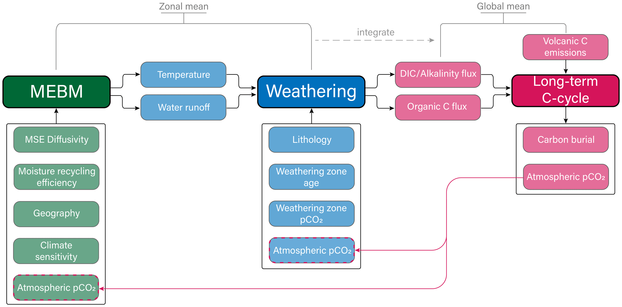
Figure 1 Coupled model schematic. The three main model components are labeled “MEBM”, “Weathering”, and “Long-term C-cycle”. Boxes with arrows pointing toward these components include terms required to initialize the model. Arrows pointing out of these components are model output. The MEBM and weathering components are solved in the zonal mean and then integrated for compatibility with the long-term C-cycle component. Atmospheric pCO₂ from the C-cycle component is used as input for the MEBM and weathering components (pink arrows) at the next time step. MSE is moist static energy, DIC is dissolved inorganic carbon, and C is carbon.

2.1 Moist Energy Balance Model (MEBM)

2.1.1 Diffusive moist static energy transport

Global climate is simulated in the zonal mean using a Moist Energy Balance Model (MEBM) following the equations and modifying the code of Roe et al. (2015) and Siler et al. (2018), which built on the earlier work of Flannery (1984) and Hwang and Frierson (2010). Zonal-mean atmospheric heating (Q_net) is balanced by poleward heat transport on long timescales (∼decadal), yielding Eq. (1):

$$\begin{array}{}\text{(1)}& Q_{\text{net}}\left(x\right)={\displaystyle \frac{\mathrm{1}}{\mathrm{2}\mathit{\pi }{a}^{\mathrm{2}}}}{\displaystyle \frac{\mathrm{d}F}{\mathrm{d}x}},\end{array}$$

where x is the sine of latitude; a is Earth's radius (m); F is the column-integrated, zonally integrated flux of atmospheric energy transport (W); and Q_net is the net downward energy flux at the top of atmosphere (TOA) (W m⁻²) (Pierrehumbert, 2010). When Q_net is positive, atmospheric energy is transported away from x, and vice versa.

Net column-integrated heating is related to the balance of non-reflected solar insolation (I) and longwave (LW) radiation by Eq. (2):

$$\begin{array}{}\text{(2)}& Q_{\text{net}}\left(x\right)=(\mathrm{1}-{\mathit{\alpha }}_{\text{S}})I-{\mathrm{LW}}_{\text{out}},\end{array}$$

where α_S is surface albedo and the (1−α_S) term represents the fraction of insolation that is not reflected back to space. The LW_out term is related to greenhouse forcing, as discussed in Sect. 2.1.3. Unless otherwise stated, I is related to the solar constant Q₀ by a second-order Legendre polynomial:

$$\begin{array}{}\text{(3)}& I=Q_{\text{0}}(\mathrm{1}-\mathrm{0.241}(\mathrm{3}{\times }^{\mathrm{2}}-\mathrm{1}\left)\right),\end{array}$$

although the code includes functionality to create time-variant insolation files consistent with paleo-conditions.

The MEBM simulates the diffusive transport of the sum of near-surface latent and sensible heat, or moist static energy (h; J kg⁻¹), which is expressed as a function of surface temperature (T):

$$\begin{array}{}\text{(4)}& h=c_{p}T+L_{\mathrm{v}}q\left(T\right),\end{array}$$

where c_p is the specific heat of air (J kg⁻¹ K⁻¹), L_v is the latent heat of vaporization (J kg⁻¹), and q is the near-surface specific humidity (kg kg⁻¹), calculated as the product of relative humidity and temperature-dependent saturation specific humidity. Relative humidity is used to partition moist static energy into its sensible and latent components and, following previous work, we assume it is constant at the global average, near-surface ocean value of 80 % (Hwang and Frierson, 2010; Siler et al., 2018). This fixed-humidity assumption is unrealistic over land, particularly in dry regions such as the subtropics, but the assumption does not interfere with the model's ability to capture the zonal-mean aridity profile. Previous work imposed spatially variable relative humidity profiles (e.g., Peterson and Boos, 2020), but selecting such a profile and how it changes with global climate introduces numerous free parameters. Instead, the Hadley cell parameterization introduced in Siler et al. (2018) (see Eq. 7 and the Supplement) retains critical features of the zonal-mean aridity profile – such as the arid subtropics – and its response to climate while also permitting the simplifying assumption of a fixed global humidity value.

Moist static energy (MSE) is transported down-gradient (poleward) following

$$\begin{array}{}\text{(5)}& F\left(x\right)=-{\displaystyle \frac{\mathrm{2}\mathit{\pi }{p}_{\mathrm{s}}}{g}}D(\mathrm{1}-x^{\mathrm{2}}){\displaystyle \frac{\mathrm{d}h}{\mathrm{d}x}},\end{array}$$

where p_s is the surface atmospheric pressure (Pa), g is gravitational acceleration (m s⁻²), and D is a zonally constant diffusivity coefficient (m² s⁻¹).

Equations (1) and (5) can be combined as follows:

$$\begin{array}{}\text{(6)}& Q_{\text{net}}\left(x\right)=-{\displaystyle \frac{p_{\mathrm{s}}}{g{a}^{\mathrm{2}}}}D{\displaystyle \frac{\mathrm{d}}{\mathrm{d}x}}\left[\left(\mathrm{1}-x^{\mathrm{2}}\right){\displaystyle \frac{\mathrm{d}h}{\mathrm{d}x}}\right].\end{array}$$

However, down-gradient MSE transport is not valid in the tropics where Hadley circulation promotes the up-gradient transport of latent heat. With the Hadley cell parameterization of Siler et al. (2018), MSE fluxes are partitioned into a tropical Hadley contribution (F_HC) and an extratropical eddy contribution (F_eddy) based on a Gaussian weighting function. Net moist static energy transport in the Hadley cell is down-gradient, but the latent component of MSE (F_HC,q) is transported up-gradient following

$$\begin{array}{}\text{(7)}& F_{\text{HC,q}}\left(x\right)=-\mathit{\psi }\left(x\right)L_{v}q\left(x\right),\end{array}$$

where ψ is the southward mass transport in the Hadley cell's lower branch (which equals the northward transport of the upper branch by mass balance). The reader is referred to Siler et al. (2018) and the Supplement of this article for further details regarding the Hadley cell parameterization.

Finally, by mass balance, the difference between evaporation and precipitation (E−P) is set equal to the divergence of the latent component of the MSE flux.

2.1.2 Partitioning P and E and parameterizing for land

The divergence of the latent heat flux balances the difference in evaporation and precipitation, or E−P, constraining a critical component of the hydrologic cycle that links hydroclimate with the carbon cycle. However, knowledge of E−P is not sufficient to quantify E and P fluxes – doing this requires constraining either E or P. We adopt the equation for oceanic evaporation of Siler et al. (2019):

$$\begin{array}{}\text{(8)}& E={\displaystyle \frac{R_G\left(x\right)\mathit{\theta }\left(x\right)+{\mathit{\rho }}_{\text{air}}{c}_p(\mathrm{1}-\mathrm{rh})C_{H}u\left(x\right)}{\mathit{\theta }\left(x\right)+\frac{c_p}{L_{v}q*\left(x\right)}}}.\end{array}$$

Here, R_G is an idealized latitudinal profile of the difference between radiative forcing and the ocean heat uptake response (W m⁻²), θ is a temperature-dependent Clausius–Clapeyron scaling factor as in Siler et al. (2018, 2019) (we use θ instead of α to avoid confusion with albedo), ρ_air is the near-surface air density (kg m³), rh is relative humidity, C_H is a drag coefficient, q^* is saturation specific humidity, and u is an idealized surface wind speed profile (m s⁻¹). Inputs for the terms defined in Eq. (8) can be found in the Supplement. We note that Eq. 8 gives E in units of watts per square meter (W m⁻²), which we convert to meters per year (m yr⁻¹) to simplify discussion. In this work, idealized profiles of R_G and u (based on Siler et al., 2018, 2019) are constant across simulations. In future work, these profiles could be designed to vary with continental geography and climate.

As discussed earlier, the spatial profile of E−P hinges on assumptions that are based on oceanic conditions (such as constant relative humidity), but it also captures the general trends on land. For example, E−P is generally negative in the tropics and middle to high latitudes and positive in the drier subtropics. However, on decadal timescales on land, E is limited by P such that E−P is always ≤0. In order to calculate terrestrial runoff (an input for the exogenic carbon cycle module), we impose this mass balance with the Budyko hydrologic balance framework (Broecker, 2010; Budyko, 1974; Fu, 1981; Koster et al., 2006; Roderick et al., 2014; Zhang et al., 2004). We calculate runoff as a fraction of precipitation using the Budyko formulation from Fu (1981):

$$\begin{array}{}\text{(9)}& \begin{array}{rl}{k}_{\text{run}}\left(x\right)& =\mathrm{1}-{\displaystyle \frac{\mathrm{ET}\left(x\right)}{P\left(x\right)}}=-{\displaystyle \frac{E_{\mathrm{0}}\left(x\right)}{P\left(x\right)}}\\ & +{\left[\mathrm{1}+{\left({\displaystyle \frac{E_{\mathrm{0}}\left(x\right)}{P\left(x\right)}}\right)}^{\mathit{\omega }}\right]}^{\mathrm{1}/\mathit{\omega }}.\end{array}\end{array}$$

In this formulation, k_run is restricted to [0,1], ET is evapotranspiration, E₀ is potential evaporation, and ω is a non-dimensional free parameter with bounds [1,∞) that determines the proximity of ET to its theoretical limits (P or E₀ when P<E₀ and P>E₀, respectively). Each value of ω defines a Budyko curve, with higher values producing a curve where evapotranspiration lies closer to the energy and water limits (E₀ and P, respectively). We set ω equal to the global mean value of 2.6 (Budyko, 1974; Zhang et al., 2004; Greve et al., 2015) unless otherwise stated. We also assume that ocean evaporation is equal to potential evapotranspiration, setting E₀ equal to E. The k_run term is then used to partition precipitation into runoff and evaporation:

$$\begin{array}{}\text{(10)}& q_{\text{land}}\left(x\right)=k_{\text{ice}}\left(x\right)k_{\text{run}}\left(x\right)P\left(x\right),\end{array}$$

where q_land is terrestrial runoff (output in meters per year after converting P to the same units), not to be confused with Q_net, a radiative forcing term in Eq. (1). The k_ice term is a coefficient that sets the “effective runoff” that is relevant for rock weathering. We define k_ice based on whether a grid cell is ice-free or glaciated using

$$\begin{array}{}\text{(11)}& k_{\text{ice}}\left(x\right)=\left\{\begin{array}{ll}\mathrm{1}& \text{if }x\text{ is ice-free}\\ [\mathrm{0},\mathrm{1}]& \text{if }x\text{ is glaciated}.\end{array}\right.\end{array}$$

Unless otherwise stated, k_ice=0 for glaciated grid cells (the default case). We demonstrate the model sensitivity to the range of glaciated k_ice values in Sect. 4.

2.1.3 Greenhouse forcing

Greenhouse gas forcing in our model is driven by the partial pressure of atmospheric pCO₂ (ppmv). Higher pCO₂ decreases the outgoing longwave flux (LW_out; W m⁻²) which is assumed to be linearly related to temperature (Budyko, 1969; Koll and Cronin, 2018) as follows:

$$\begin{array}{}\text{(12)}& {\mathrm{LW}}_{\text{out}}\left(x\right)=A+BT\left(x\right).\end{array}$$

Here, T is surface temperature (K), B is a coefficient that captures the Planck feedback (W m⁻² K⁻¹), and A (W m⁻²) is a constant that depends on CO₂:

$$\begin{array}{}\text{(13)}& A=C_{\mathrm{LW}}-M\ln (p{\mathrm{CO}}_{\mathrm{2},t}/p{\mathrm{CO}}_{\mathrm{2},t\mathrm{0}}).\end{array}$$

In the expression above, C_LW and M (both W m⁻²) are tunable parameters that determine the climate sensitivity to pCO₂. pCO_2,t is the partial pressure of CO₂ (ppmv) at some time, which is divided by the reference pCO₂, pCO_2,t0. The baseline pCO₂ is set at 280 ppmv, with the parameters C_LW, M, and B given in Table S1 in the Supplement.

2.1.4 Domain boundary conditions

We prescribe the latitudinal distribution of continents and use this distribution to calculate Earth surface albedo. We assign three albedo values – ocean albedo, land albedo, and ice albedo – and calculate the average albedo at each latitudinal node by the weighted average of land and ocean area. Ice sheets in our model appear at a temperature threshold (e.g., North et al., 1981) (T_ice, set at −5 ^∘C) such that the albedo for any node with T<T_ice is equal to the ice albedo (with no dependence on land or ocean values).

The set of MEBM equations can be solved as a boundary value problem, and we use the “bvpcol” function from the “bvpSolve” package in R (Mazzia et al., 2014) (see the Supplement). We prescribe a zero-flux boundary condition, assuming the flux of moist static energy at both poles is zero. We also prescribe initial temperature guesses for each pole (T_north and T_south). The temperature guesses can lead to multi-stability in model solutions: for the same forcing, a colder temperature guess might yield a stable icehouse, whereas a warmer guess might yield a stable greenhouse. In this paper, we use the same temperature guess for every time step of a given simulation to enforce a mono-stable climate (a unique climate solution for every pCO₂).

2.2 Weathering

We calculate solute concentrations for bicarbonate carbon [C] (mol L⁻¹) derived from silicate and carbonate weathering at each latitudinal node using each node's surface temperature (T) and terrestrial runoff (q_land). T and q_land are derived from the MEBM (see Sect. 2.1.2).

The value of [C]_sil is calculated using equations modified from Maher and Chamberlain (2014) (similar to the “MAC” model in other works; Baum et al., 2022; Graham and Pierrehumbert, 2020). These equations permit us to explicitly incorporate the effect of T, q_land, and weathering-zone pCO₂ – variables that are all influenced by atmospheric pCO2 and climate – on [C]_sil:

$$\begin{array}{}\text{(14)}& {\left[\mathrm{C}\right]}_{\text{sil }}={\left[\mathrm{C}\right]}_{\text{sil,eq }}\left({\displaystyle \frac{\frac{D_{\mathrm{w}}}{q_{\text{land}}}}{\mathrm{1}+\frac{D_{\mathrm{w}}}{q_{\text{land}}}}}\right).\end{array}$$

Here, [C]_sil,eq is the maximum equilibrium concentration of silicate-derived bicarbonate (Maher, 2011) and D_w is the Damköhler weathering coefficient (m yr⁻¹), which is a term that encapsulates the reactivity of the weathering zone and the time required to reach equilibrium. Following Maher and Chamberlain (2014), we define D_w as follows:

$$\begin{array}{}\text{(15)}& D_{\mathrm{w}}={\displaystyle \frac{L_{\mathit{\varphi }}{r}_{max}\frac{\mathrm{1}}{\mathrm{1}+t_{\text{wz}}m{k}_{\text{eff}}A}}{[C{]}_{\text{sil, eq}}}},\end{array}$$

where Lϕ is the reactive length scale (m), held constant; r_max is the theoretical maximum reaction rate (mol L⁻¹ yr⁻¹); t_wz is the age of the weathering zone (yr) and is a key variable describing the reactivity of the weathering zone; m is the molar mass of weathering minerals (g mol⁻¹); A is the specific surface area of minerals undergoing weathering (m² g⁻¹); and k_eff is the effective reaction rate constant (mol m² yr⁻¹). The r_max term is scaled with the effective reaction rate constant as follows:

$$\begin{array}{}\text{(16)}& r_{max}=r_{\text{max,ref}}{\displaystyle \frac{k_{\text{eff}}}{k_{\text{eff,ref}}}},\end{array}$$

where r_max,ref and k_eff,ref are reference values taken from Maher and Chamberlain (2014) to be $\mathrm{1085}\times {\mathrm{10}}^{-\mathrm{6}}$ µmol L⁻¹ yr⁻¹ and $\mathrm{8.7}\times {\mathrm{10}}^{-\mathrm{6}}$ mol m⁻² yr⁻¹, respectively. The effective reaction rate constant is, itself, related to k_eff,ref by an Arrhenius function that describes the temperature dependency of reaction rates (Brady, 1991; Kump et al., 2000):

$$\begin{array}{}\text{(17)}& k_{\text{eff}}=k_{\text{eff,ref}}{e}^{\left[\left(\frac{\mathrm{Ea}}{R_g}\right)\left(\frac{\mathrm{1}}{T_{\mathrm{0}}}-\frac{\mathrm{1}}{T}\right)\right]},\end{array}$$

where R_g is the universal gas constant (J K⁻¹ mol⁻¹) (distinct from R_G in Eq. 8), Ea is the activation energy (J mol⁻¹), and T₀ is the reference temperature associated with k_eff,ref.

Lastly, [C]_sil,eq is modified by the availability of reactant, which is assumed to be primarily CO₂ here. We calculate this effect as a function of weathering-zone pCO₂ assuming open-system CO₂ dynamics, following Winnick and Maher (2018):

$$\begin{array}{}\text{(18)}& {\left[\mathrm{C}\right]}_{\text{sil,eq}}={\left[\mathrm{C}\right]}_{\text{sil,eq,0}}{\left(R_{{\mathrm{CO}}_{\mathrm{2}},\mathrm{wz}}\right)}^{\mathrm{0.316}},\end{array}$$

where [C]_sil,eq,0 is the pre-perturbation initial value of [C]_sil,eq. $R_{{\mathrm{CO}}_{\mathrm{2}},\mathrm{wz}}$ is the ratio of weathering-zone pCO₂ at time t (WZ${}_{{\mathrm{CO}}_{\mathrm{2}}}$) to the initial weathering-zone pCO₂ pre-perturbation (WZ${}_{{\mathrm{CO}}_{\mathrm{2}},\mathrm{0}}$). The exponent value of 0.316 is derived by Winnick and Maher (2018) based on the net weathering stoichiometry for an open-system scaling relationship for the dissolution of plagioclase feldspar (An₂0) and precipitation of halloysite. Depending on the primary lithology and secondary mineral precipitated, this exponent can vary from ∼0.25 to 0.7 (see Winnick and Maher, 2018, their Table 1). This average stoichiometry represents an average granodiorite continental crust (e.g., Maher, 2010, 2011; Maher and Chamberlain, 2014). We calculate $R_{{\mathrm{CO}}_{\mathrm{2}},\mathrm{wz}}$ using a formulation proposed by Volk (1987) that links weathering-zone pCO₂ with the primary source of that CO₂, which is aboveground terrestrial gross primary productivity (GPP; kg m⁻² yr⁻¹). Here, WZ${}_{{\mathrm{CO}}_{\mathrm{2}}}$ is calculated using an equation that links GPP, CO₂ fertilization of GPP, and weathering-zone CO₂:

$$\begin{array}{}\text{(19)}& {\mathrm{WZ}}_{{\mathrm{CO}}_{\mathrm{2}}}=p{\mathrm{CO}}_{\mathrm{2}}+R_{\text{GPP}}\left({\mathrm{WZ}}_{{\mathrm{CO}}_{\mathrm{2}},\mathrm{0}}-p{\mathrm{CO}}_{\mathrm{2},\mathrm{0}}\right),\end{array}$$

where R_GPP is the ratio of GPP at time t to the pre-perturbation GPP (GPP₀) and the last term on the right-hand side of the equation ensures that WZ${}_{{\mathrm{CO}}_{\mathrm{2}}}$ is always greater than atmospheric pCO₂. The GPP is calculated using a Michaelis–Menten formulation:

$$\begin{array}{}\text{(20)}& \mathrm{GPP}={\mathrm{GPP}}_{max}\left[{\displaystyle \frac{p{\mathrm{CO}}_{\mathrm{2}}-p{\mathrm{CO}}_{\mathrm{2},min}}{p{\mathrm{CO}}_{\mathrm{2},\text{half}}+\left(p{\mathrm{CO}}_{\mathrm{2}}-p{\mathrm{CO}}_{\mathrm{2},min}\right)}}\right].\end{array}$$

Here, GPP_max is the maximum possible global terrestrial GPP, pCO_2,min is the pCO₂ at which photosynthesis is balanced exactly by photorespiration, and pCO_2,half is the pCO₂ at which GPP is equivalent to 50 % GPP_max:

$$\begin{array}{}\text{(21)}& p{\mathrm{CO}}_{\mathrm{2},\text{half}}=\left({\displaystyle \frac{{\mathrm{GPP}}_{max}}{{\mathrm{GPP}}_{\mathrm{0}}}}-\mathrm{1}\right)\left(p{\mathrm{CO}}_{\mathrm{2},\mathrm{0}}-p{\mathrm{CO}}_{\mathrm{2},min}\right).\end{array}$$

We choose a pCO_2,min of 100 ppm based upon evidence for widespread CO₂ starvation at the Last Glacial Maximum (LGM) (Prentice and Harrison, 2009; Scheff et al., 2017), which had an atmospheric pCO₂ of 180 ppm. We also assume that GPP_max is equal to twice GPP₀, although our results are insensitive to this parameter. Lastly, we assume that WZ${}_{{\mathrm{CO}}_{\mathrm{2}},\mathrm{0}}$ is a factor of 10 larger than atmospheric pCO_2,0 given evidence that soil pCO₂ is typically elevated above atmospheric levels by approximately an order of magnitude (Brook et al., 1983). While this formulation offers a crude accounting of the effect of GPP on weathering-zone pCO₂, it is not strictly internally consistent. Setting pCO₂ in equation 20 equal to pCO_2,half does not guarantee a GPP value that is half of GPP_max, although it will yield a value close enough that the effect on the model results is negligible.

We use this set of equations to calculate silicate and carbonate weathering. Carbonate weathering is scaled to silicate weathering such that carbonate D_w is 2.5 times greater than silicate D_w and maximum equilibrium concentrations of carbonate-derived bicarbonate are 2 times greater than [C]_sil,eq (Lasaga, 1984; Bluth and Kump, 1994; Morse and Arvidson, 2002; Ibarra et al., 2017; Gaillardet et al., 2019). The concentrations calculated above are translated into global weathering fluxes (F_w):

$$\begin{array}{}\text{(22)}& F_{\text{w,sil/carb}}=q_{\text{land}}\left(x\right)\left[C{]}_{\text{sil/carb}}\right(x\left)A_{\text{land}}\right(x)W_{\text{sil/carb}},\end{array}$$

where x is the sine of latitude following the MEBM grid spacing; the subscripts sil and carb refer to silicate and carbonate weathering, respectively; A_land is the land area (m²); and W is a scalar used to enforce mass balance and is held constant throughout a run. The W parameter is a global constant and differs for carbonate vs. silicate weathering. We calculate W_sil/carb during model initialization to ensure that the global sum of carbon burial fluxes equals the sum of input fluxes, such that the model starts in a steady state. For silicate weathering, W_sil scales with F_w,sil such that F_w,sil equals F_volc at initialization. The W_sil scalar can also be thought of as loosely representing a global SiO₂:HCO₃ ratio that translates silica fluxes to inorganic carbon fluxes. This translation is necessary because these weathering equations – and the associated parameters – in Maher and Chamberlain (2014) were originally derived for Si fluxes, rather than C (or alkalinity) fluxes. For modern basaltic and granitic catchments, Ibarra et al. (2016) demonstrated that [C]_sil,eq,0 scales proportional to weathering stoichiometry, as predicted by Winnick and Maher (2018), and D_w scales with some bias towards more chemostatic (higher D_w) values in Si compared with alkalinity (Moon et al., 2014). Because W_sil determines the sensitivity of weathering fluxes to changes in runoff and concentration, it also influences the strength of the silicate weathering feedback (defined as the change in weathering fluxes per change in atmospheric CO₂). Similarly, W_carb is determined by scaling the sum of the carbonate weathering fluxes at each node such that these fluxes equal the estimate of the carbonate weathering flux in Wallmann (2001), forcing the model to start in a steady state. Importantly, because W_sil/carb depends on A_land, continental geography has an indirect effect on the strength of the weathering response to climate by Eq. (22).

2.3 Carbon cycle

The carbon cycle model follows other one-box models that are commonly employed for tracking long-term (i.e., on timescales of >10⁵ years) changes to the carbon cycle and δ¹³C (e.g., Berner, 1991; Kump and Arthur, 1999). The input fluxes of C into the ocean–atmosphere system include volcanism and solid-Earth degassing (F_volc), organic carbon weathering (F_w,org), and carbonate weathering (F_w,carb), and the output fluxes are the burial of organic carbon and carbonate carbon in marine sediments (F_b,org and F_b,carb, respectively, all in moles per year). The input fluxes have an associated δ¹³C (i.e., ${\mathit{\delta }}^{\mathrm{13}}{\mathrm{C}}_{\text{volc}}=-\mathrm{5}\mathrm{‰}$, δ¹³C_w,carb=0 ‰). δ¹³C_w,org is set to ensure isotopic mass balance at the first time step by setting the left side of Eq. (24) (below) to zero and rearranging to solve for δ¹³C_w,org. The δ¹³C values of the output fluxes are determined by a fixed fractionation factor relative to the global average of the ocean–atmosphere system ($\mathit{ϵ}={\mathit{\delta }}^{\mathrm{13}}{\mathrm{C}}_{\text{output flux}}-{\mathit{\delta }}^{\mathrm{13}}$C, i.e., ϵ_b,org and ϵ_b,carb). The subsequent mass balance equation for the total mass of carbon in the one-box ocean–atmosphere (M_C) is

$$\begin{array}{}\text{(23)}& {\displaystyle \frac{\mathrm{d}{M}_C}{\mathrm{d}t}}=F_{\text{volc}}+F_{\text{w,org}}+F_{\text{w,carb}}-F_{\text{b,org}}-F_{\text{b,carb}}.\end{array}$$

The associated isotope mass balance equation for the carbon isotope value of the ocean–atmosphere system (δ¹³C) is

$$\begin{array}{}\text{(24)}& \begin{array}{rl}{\displaystyle \frac{\mathrm{d}{\mathit{\delta }}^{\mathrm{13}}\mathrm{C}}{\mathrm{d}t}}{M}_{\mathrm{C}}& =F_{\text{volc}}({\mathit{\delta }}^{\mathrm{13}}{\mathrm{C}}_{\text{volc}}-{\mathit{\delta }}^{\mathrm{13}}\mathrm{C})+F_{\text{w,org}}({\mathit{\delta }}^{\mathrm{13}}{\mathrm{C}}_{\text{w,org}}\\ & -{\mathit{\delta }}^{\mathrm{13}}\mathrm{C})+F_{\text{w,carb}}({\mathit{\delta }}^{\mathrm{13}}{\mathrm{C}}_{\text{w,carb}}-{\mathit{\delta }}^{\mathrm{13}}\mathrm{C})\\ & -F_{\text{b,org}}{\mathit{ϵ}}_{\text{b,org}}-F_{\text{b,carb}}{\mathit{ϵ}}_{\text{b,carb}}.\end{array}\end{array}$$

The last term in Eq. (24) goes to zero, as we assume that ϵ_b,carb is zero (δ¹³C of carbonate burial equals that of the dissolved inorganic carbon, DIC, pool). While δ¹³C is a useful tracer for carbon cycle dynamics, we focus on climate–carbon interactions in this paper, where the δ¹³C results are less informative. For simplicity, the organic carbon burial flux (F_b,org) is scaled to the carbonate burial flux (F_b,carb) by $F_{\text{b,org,t}}=F_{\text{b,org,i}}\times (F_{\text{b,carb,t}}/F_{\text{b,carb,i}})$, where the subscripts t and i refer to some point in time and the initial condition, respectively (Caves Rugenstein et al., 2019; Ridgwell, 2003). The carbonate carbon burial flux is a function of the calcite saturation index (Ω_calcite), such that $F_{\text{b,carb,t}}=F_{\text{b,carb,i}}\times {\mathrm{\Omega }}_{\text{t}}/{\mathrm{\Omega }}_{\text{i}}$. The Ω_calcite term is calculated as a function of the carbonate system (Zeebe and Wolf-Gladrow 2001), accounting for the concentrations of [Mg²⁺] and [Ca²⁺] using the equations of Zeebe and Tyrrell (2019). The alkalinity reservoir in the ocean, M_Alk, is related to the fluxes as follows:

$$\begin{array}{}\text{(25)}& {\displaystyle \frac{\mathrm{d}{M}_{\text{Alk}}}{\mathrm{d}t}}=F_{\text{w,sil}}+F_{\text{w,carb}}-F_{\text{b,carb}},\end{array}$$

where F_w,sil is the silicate weathering flux. Parameter values and references can be found in Table S3, and specific details about key parameters are described below.

To achieve mass balance for M_C and M_Alk, F_volc must equal F_w,sil at steady state. The global temperature at Earth's surface (T_a) is calculated by integrating the MEBM temperature results weighted by land area and is then used to set the global mean ocean temperature T_o by assuming that the mean ocean temperature is 10 ^∘C colder than T_a (Key et al., 2004). To solve the initial carbonate system and associated initial M_C and M_Alk, the initial ocean pH, pCO₂, T_o, salinity (35 psu), mean ocean pressure (300 bar), and geochemical composition of seawater (i.e., Ca $=\mathrm{15}\times {\mathrm{10}}^{-\mathrm{3}}$, Mg $=\mathrm{48.5}\times {\mathrm{10}}^{-\mathrm{3}}$, and ${\mathrm{SO}}_{\mathrm{4}}^{\mathrm{2}-}=\mathrm{28.2}\times {\mathrm{10}}^{-\mathrm{3}}$ mol L⁻¹) are input into the speciation equations of Zeebe and Wolf-Gladrow (2001), modified by Zeebe and Tyrrell (2019) to account for variable ocean chemistry (see Table S3).

2.4 Coupled climate–carbon cycle model initialization and integration

We first initialize the MEBM and carbon cycle boundary conditions including the initial global carbon cycle fluxes (see Tables S3 and S1). The carbon cycle is parameterized to start in a steady state (inputs of carbon equal the outputs). We begin by simulating the initial climate state by prescribing an initial atmospheric pCO₂ to force the MEBM. This same pCO₂ is used, along with an initial pH (Table S3), to speciate the carbon cycle (Zeebe and Wolf-Gladrow, 2001). Temperature and runoff from this initial climate state are used to calculate weathering fluxes following Eq. (22), where the scalar W is set to one. We then calculate the scalars for carbonate and silicate weathering as follows:

$$\begin{array}{}\text{(26)}& {\displaystyle }{W}_{\text{sil}}={\displaystyle \frac{F_{\text{volc, ss}}}{\sum F_{\text{w,sil,i}}}},\text{(27)}& {\displaystyle }{W}_{\text{carb}}={\displaystyle \frac{F_{\text{w,carb, ss}}}{\sum F_{\text{w,carb,i}}}}.\end{array}$$

Here, i refers to the initial, unscaled fluxes; the subscript ss refers to the steady-state fluxes; and ∑ denotes the global sum (note that the zonal-mean grid is an equal-area grid).

We couple the MEBM to the long-term carbon cycle module by solving the MEBM at each time step within the carbon cycle solver. First, the carbon cycle module solves for atmospheric pCO₂ for the given time step using the mass balance of DIC and alkalinity and the carbonate speciation described in the previous section. This pCO₂ value, along with the required polar temperature guesses (discussed in Sect. 2.1.4), is used to force the MEBM. Some temperature guesses at low pCO₂ levels will lead to no stable solution or a “snowball Earth” configuration where the entire planet is glaciated (see the Supplement). For either of these outcomes, we rerun the MEBM using temperature guesses that are a small step (usually ∼0.5 ^∘C) toward a warmer direction. This is repeated until the MEBM finds a stable solution that is not a fully glaciated planet (usually less than three steps are needed until such a solution is reached). We use this method for avoiding snowball states because the range of pCO₂ forcing in our simulations is above the lowest pCO₂ concentrations of the Quaternary and, therefore, a fully glaciated planet is unreasonable, although users may easily turn off this snowball-avoiding feature. The fact that fully glaciated solutions are usually not robust to small perturbations in the temperature guess indicates that the snowball scenario itself is not robust. Once a stable solution is found, the latitudinally resolved hydrological and temperature output from the MEBM are used to solve for the silicate and carbonate weathering fluxes. These weathering fluxes as well as any perturbations to the input carbon fluxes (such as via changes in F_volc) then drive the response of the long-term carbon cycle including the updated marine carbonate speciation based on DIC and total alkalinity.

2.5 Model assumptions

A number of model processes are not fully coupled among all modules. These processes are parameterized with simplifying assumptions for the purpose of this work, but they could be coupled in the future (albeit with additional parameters). We detail these assumptions below.

We assume that no weathering occurs beneath ice sheets such that the weathering fluxes at glaciated latitudes are zero because k_ice is zero. While weathering rates in glacial catchments can be high, it remains unclear whether glaciated catchments are a net source or sink of CO₂ on long timescales (Torres et al., 2017). Our assumption of no weathering beneath ice sheets is consistent with previous modeling work (e.g., Zachos and Kump, 2005; Pollard et al., 2013) and has two main effects on our model. First, when a simulation transitions from a greenhouse to an icehouse there is a reduction in weathering due to cooler climate conditions and decreasing precipitation and an additional reduction due to ice sheet growth. Second, when initializing the model in an icehouse state, the weathering scalar term, W (calculated at initialization), is higher because the denominator in Eqs. (26) and (27) is lower due to ice coverage. We test the sensitivity of this assumption to our results in our model experiments (next section).

We also neglect the effect of ice coverage on global eustatic sea level in our model. Terrestrial ice coverage decreases sea level, exposing more land area and potentially increasing global weathering. This effect would counteract the effect of ice coverage decreasing the weatherable land area (discussed above). However, accounting for the effect of sea level on exposed land area requires constraints on hypsometry (at least near the coasts) as well as ice volume, both of which are absent from our one-dimensional model framework. Moreover, any increase in silicate weathering due to sea level fall is expected to be small or negligible because exposed shelves are likely to consist of carbonates and organic- and clay-rich sediment, not primary silicate minerals (Berner, 1994; Gibbs and Kump, 1994; Kump and Alley, 1994), and may act as a source of atmospheric CO₂ (Kölling et al., 2019).

Part of the weathering module scales silicate and carbonate solute concentrations with weathering-zone pCO₂. This weathering-zone pCO₂ is calculated from several global parameters, including atmospheric pCO₂ and GPP, and ignores local climatic influences on weathering-zone pCO₂. Soil pCO₂ is known to vary with local climate (Brook et al., 1983; Cotton and Sheldon, 2012; Cotton et al., 2013) and decoupling weathering-zone pCO₂ from local climate is clearly a major simplification. Nevertheless, there remains substantial uncertainty regarding how soil-zone pCO₂ will change in response to warming and rising atmospheric pCO₂ (Terrer et al., 2021). This uncertainty motivates our use of the simpler, global model for GPP following Volk (1987, 1989). Given that [C] is, in our model, only sensitive to weathering-zone pCO₂ to the power of 0.316 (Winnick and Maher, 2018), the lack of a coupling between local climate and weathering-zone pCO₂ is likely to have a muted effect on our predicted [C]_sil and [C]_carb.

An additional assumption in our model is that the negative feedback that regulates long-term climate is terrestrial weathering (i.e., continental silicate and carbonate weathering). For example, we have not explicitly included seafloor basalt weathering fluxes as a silicate weathering flux separate from terrestrial silicate weathering fluxes, although recent work has suggested that seafloor basalt weathering may be a substantial portion of the global weathering flux, particularly during hothouse climates (Coogan and Gillis, 2013, 2018). Further, we assume that the positive and negative feedbacks of the organic carbon cycle, other than burial, are outpaced by the silicate weathering feedback on climate. Recent work has suggested that organic carbon weathering may be linked to climate (Hilton and West, 2020). This coupling between climate and organic carbon weathering – as well as links to marine productivity and organic carbon export and burial in marine sediments – remains an area of intensive research, and introducing carbon cycle feedbacks on climate via the organic carbon cycle represents a promising avenue for further work.

We note that, in our model, there is a simplified coupling between climate and organic carbon burial (F_b,org). F_b,org is linked to F_b,carb, which is sensitive to Ω and, hence, to atmospheric pCO₂ and to F_w,carb, whereas other frameworks simulate organic carbon burial more mechanistically, explicitly capturing features absent from our model such as diagenesis, redox-dependence of phosphorus cycling, and more (Hülse et al., 2018). For simplicity, we assume constant organic carbon weathering in this paper, which can lead to slight ($<\sim \mathrm{5}\mathit{\%}$) imbalances in organic carbon cycling when the initial and final model states $\left(\frac{\mathrm{d}{M}_C}{\mathrm{d}t}=\mathrm{0}\right)$ have different climates. These imbalances are small enough to have a negligible effect on atmospheric pO₂ for the timescales of our simulations.

3 Model experiments

We run a series of experiments with the CH2O-CHOO TRAIN model to demonstrate its features and sensitivity to key climate variables. The goal of these experiments is twofold: we aim to illustrate the importance of the spatial (zonal-mean) dimension in climate–carbon cycle interactions and to demonstrate how features of the climate system governing temperature and water cycling can impact the long-term carbon cycle. To this end, we use different continental configurations for each set of experiments to emphasize how spatially variable temperature and runoff responses can impact weathering fluxes (see Fig. 2 for geography schematics and descriptions). These experiments are not meant to be an exhaustive sensitivity analysis of the model. Instead, they provide a baseline for model performance and they illustrate climate–carbon cycle interactions that are absent in many simpler models or are emergent properties of more complex frameworks.

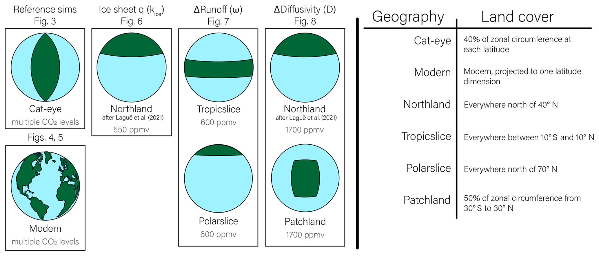
Figure 2 List of continental configurations. Each box refers to a set of model experiments, labeled with the associated figures. Maps are shown in two dimensions for convenience, but simulations consider only one dimension in the zonal-mean framework. A plain-language description of land cover is given in the table to the right. Note that changing land cover will not necessarily impact long-term carbon cycling because the steady-state carbon cycle fluxes are user-defined.

In our first set of experiments, our reference simulations, we begin by analyzing the spatial pattern of climate and weathering for a “Cat-eye” geography – a constant land fraction at each latitude – under different glacial conditions and pCO₂ levels. Zonal-mean albedo is constant in this configuration, allowing us to explore the basic spatial patterns of temperature, hydroclimate (precipitation and evaporation), and silicate weathering as well as their response to greenhouse forcing without much spatial complexity from the distribution of land. Next, we test the model using modern geography and imposing a perturbation similar to the Paleocene–Eocene Thermal Maximum (PETM) with an injection of 5000 Pg of carbon with a δ¹³C value of −20 ‰ to the atmosphere over 10 000 years (Cui et al., 2011; Frieling et al., 2016; Gutjahr et al., 2017). This simulation is used for a basic comparison of the timescale of the model response with other modeling results and data.

Second, we test for interaction effects between key variables – especially climate variables – influencing the steady-state climate (that which occurs when $\frac{\mathrm{d}{M}_C}{\mathrm{d}t}=\mathrm{0}$). Interaction effects occur when the effect of changing two variables at once differs from the sum of each individual variable's effect. To test for interaction effects, we run factorial experiments testing all combinations of five variables with three possible values each (a total of 243, or 3⁵, simulations). Each simulation starts from the same initial climate state, is perturbed to the new state at the first time step, and is allowed 750 kyr to reach a new steady state. The initial state uses the modern geographic configuration (Fig. 2) with the default value for each unperturbed variable. We repeat these 243 simulations for two initial climate states: (1) a low-pCO₂ state with polar glaciers (350 ppmv) and (2) a high-pCO₂ state with ice-free poles (4500 ppmv).

We then turn our focus to individual variables that have spatially distinct impacts on climate and weathering. In our third set of experiments, we evaluate the model sensitivity to the effect of ice sheets on weathering by changing k_ice over glaciated regions (see Eqs. 10 and 11). In effect, this varies the weathering-effective runoff – how much of the runoff calculated from the product of k_run and P contributes to weathering at glaciated latitudes. Here, we test the model response to varying k_ice in glaciated regions between zero and one (in all other simulations, k_ice is set to zero). For these experiments, we use a “Northland” geography, inspired by Laguë et al. (2021). This configuration concentrates land at high latitudes where ice sheets can have the largest impact on weathering fluxes. A comparison to a land-free simulation shows that the Northland geography has a similar effect in our model as in Laguë et al. (2021), shifting the mean Intertropical Convergence Zone (ITCZ) southward by $\sim \mathrm{5}{}^{\circ }$ (Fig. S2). Starting from an ice-free climate for each of five glaciated k_ice values, we force an instantaneous, permanent halving of the volcanic flux. The different k_ice values have no impact on climate until the decrease in volcanism is sufficient for glaciers to form. Physically, higher k_run may represent conditions such as patchy ice cover over land or ice sheets decreasing sea level to expose weatherable continental shelf.

Fourth, we test the model response to an instantaneous change in runoff by modifying the efficiency of moisture recycling (ω in Eq. 9). The term ω determines how efficiently precipitation is partitioned into evaporation vs. runoff, with higher values of ω corresponding to more evaporation and less runoff. For this experiment, we compare a world with all land in the tropics, “Tropicslice”, to one with land concentrated at a pole, “Polarslice” (see Fig. 2 for the distinction between Polarslice and Northland), because the sensitivity of runoff and temperature to pCO₂ differs between these regions. In each geographic configuration, we change ω from the control value of 2.6 to 2.0 (increasing runoff) and to 3.5 (decreasing runoff), approximating the 25th and 75th quantiles of the global distribution of ω (Greve et al., 2015).

Finally, we test the model response to an instantaneous change in the diffusivity of moist static energy (D in Eq. 5). An increase in diffusivity tends to cool the tropics, warm the poles, and transport more moisture from the subtropics to the middle to high latitudes. To capture these spatially complex effects, we simulate a change in D for two geographies with similar global land areas: a Northern Hemisphere continent (Northland, as in the ice sheet simulations) and a patch of land that spans the tropics and subtropics (“Patchland”). Unlike the Tropicslice and Polarslice geographies, Patchland and Northland each span more than one climate zone. In these experiments, we vary D by $\sim \pm \mathrm{30}$ % from the control value of 1.06×10⁶ m² s⁻¹ (Hwang and Frierson, 2010) consistent with variations one might expect between an icehouse and a greenhouse climate (e.g., Frierson et al., 2006). To isolate the effect of D, we hold the relative partitioning of Hadley cell transport constant, although changes in temperature will impact Hadley transport through the gross moist stability term (see the Supplement).

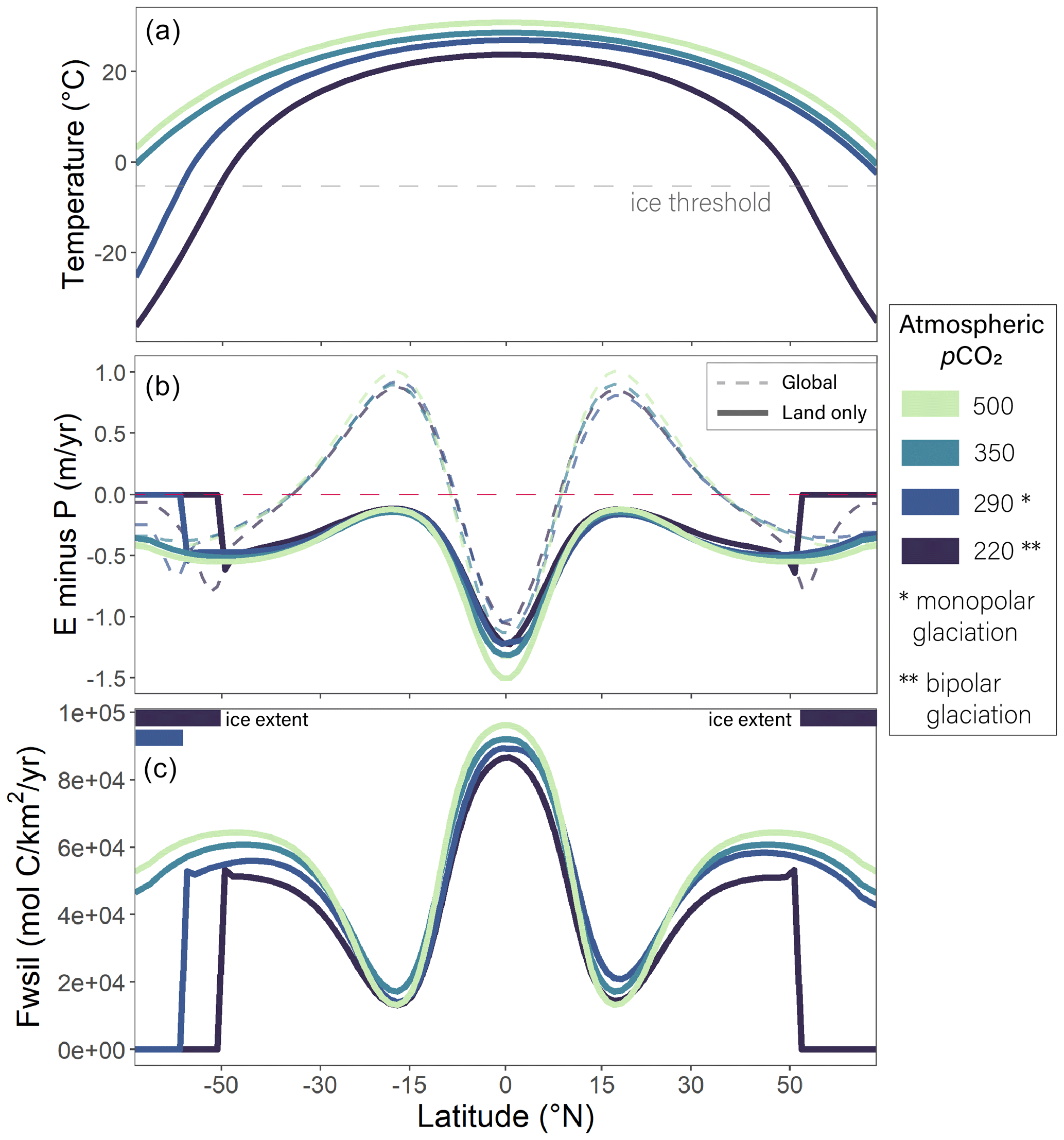
Figure 3 Reference climate state. Zonal-mean output for (a) temperature, (b) evaporation (E) minus precipitation (P), and (c) the silicate weathering rate are shown for four pCO₂ levels. Negative values of E minus P indicate more runoff. Dashed E minus P lines refer to the global pattern before the Budyko hydrologic balance framework is applied over land. The latitude axis is an equal-area grid.

4 Results

4.1 Reference simulation

We define a reference simulation with the Cat-eye geography to illustrate the one-dimensional outputs of the MEBM and weathering models (Fig. 3). Global climate transitions from a bipolar glaciation (similar to the present day) to a monopolar glaciation and, finally, ice-free as pCO₂ increases from 220 to 350 ppmv. The pCO₂ thresholds for glaciation depend on a variety of prescribed factors such as climate sensitivity as well as the geography and prescribed land, ocean, and ice albedo values. Despite the land cover and insolation forcing being meridionally symmetric about the Equator, asymmetric results such as the monopolar glaciation are still possible. The monopolar state exists because there is too much atmospheric pCO₂ to support a colder, bipolar glaciation but too little to support an ice-free world. When the land cover (and, thus, albedo) and insolation are meridionally symmetric, the pole with the lower initial temperature guess will glaciate first as the planet cools. If both temperature guesses are the same, the first pole to glaciate in the meridionally symmetric case will depend on which pole the numerical solver addresses first – that is, which pole is associated with the first guess. However, the vast majority of model cases likely involve meridional asymmetry, as no realistic continental geography is perfectly symmetric about the Equator. In such asymmetric cases, the pole that glaciates in the monopolar case is determined by the asymmetry, not the polar temperature guess and numerical configuration.

The model hydroclimate output is shown in the spatial pattern of E minus P, which balances the divergence of the latent heat flux (Fig. 3b). In the global zonal mean, P exceeds E in the tropics and middle to high latitudes, but E is greater than P in the subtropics due to the dry downwelling branches of the Hadley cell. There is an abrupt decrease in E minus P at the ice threshold due to the stepwise change in albedo, temperature, and moist static energy which forces rainout. The global temperature and hydroclimate fields shown in Fig. 3a and b ultimately determine the spatial pattern of silicate weathering (Fig. 3c). Weathering rates are highest in the tropics where temperature and runoff are high, and lowest in the subtropics where runoff is low. Whereas the broad spatial pattern of runoff sets the pattern of silicate weathering, changes in silicate weathering with climate largely respond to temperature in these simulations because the runoff response is small. For example, runoff is generally insensitive to global climate between 30 and 50^∘ latitude (north or south) (Fig. 3b), but weathering fluxes increase with pCO₂ due to the combined effect of warmer temperatures and higher soil pCO₂ (Fig. 3c). Weathering fluxes are zero for glaciated latitudes because, for these simulations, k_ice is zero.

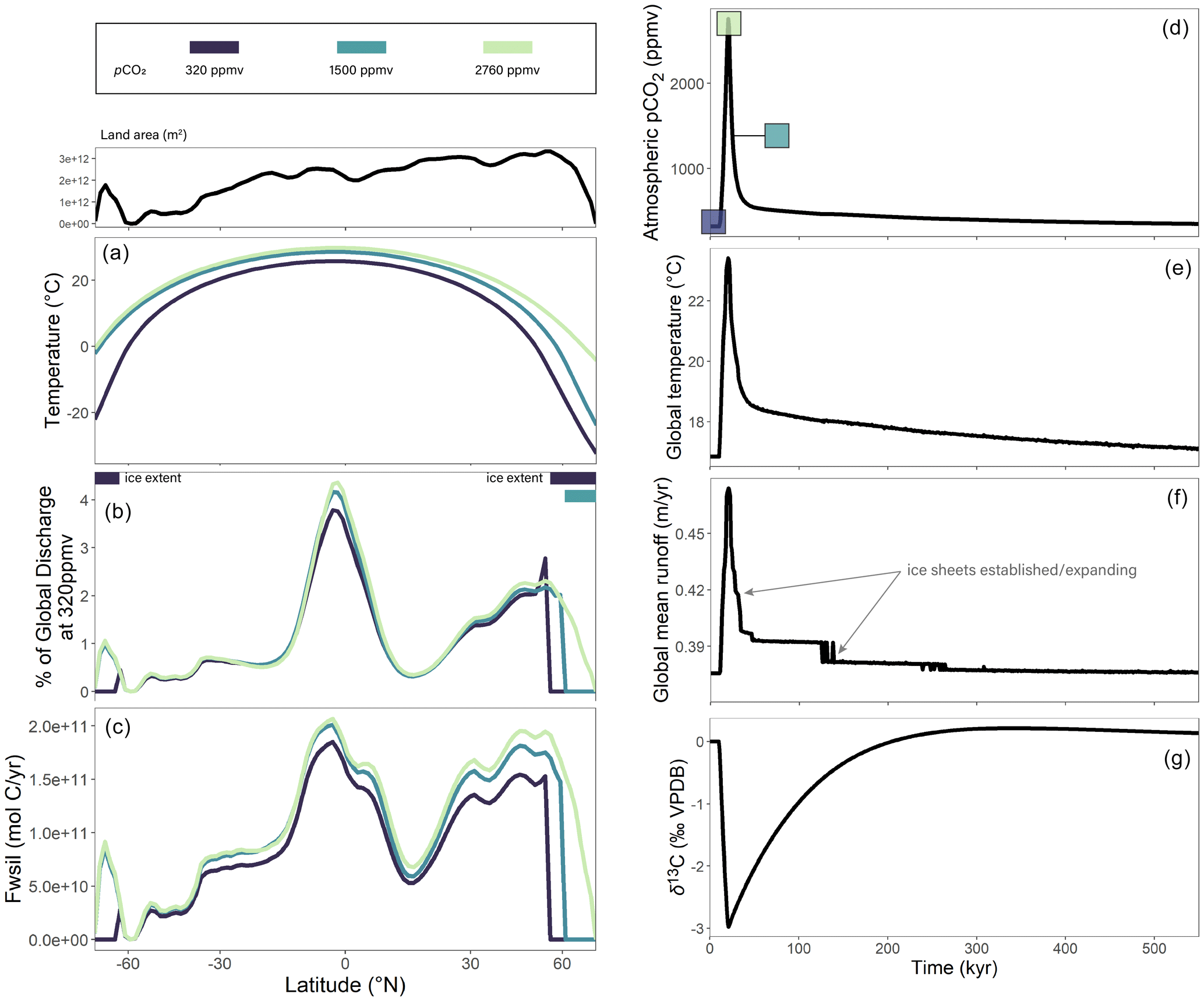
Figure 4 Abrupt warming experiment for the modern world. Zonal-mean results for (a) temperature, (b) the percent of global discharge at each equal-area latitudinal grid cell in the 320 ppmv pCO₂ simulation, and (c) the silicate weathering flux for each equal-area latitudinal grid cell at three selected time steps. The time steps in panels (a–c) correspond to the colored boxes in panel (d). The panels in the right column show the temporal evolution of (d) atmospheric pCO₂, (e) global temperature, and (f) global mean runoff as well as (g) the carbon isotope composition of the DIC pool. Arrows denote stepwise changes in runoff due to the establishment of ice sheets limiting runoff beneath them.

4.2 Response to abrupt pCO₂ increase with modern geography

Starting at 320 ppmv pCO₂ for the modern geography, the model simulates a bipolar glaciation with the spatial pattern of global discharge and silicate weathering closely matching that of continental area and the zonal-mean water balance (Fig. 4a, b, c). Today, mean air temperatures in the South Pole are lower than in the North Pole, whereas the model finds a cooler North Pole. This discrepancy is probably due to the fact that we do not account for factors such as ocean circulation, spatial variability in land albedo, cloud feedbacks, cloud albedo, topography, or a glacier height mass balance feedback. For example, in the model more land in the Northern Hemisphere leads to higher albedo and a cooler climate, although recent work shows that more cloud cover in the Southern Hemisphere compensates for the effect of Northern Hemisphere land, causing both hemispheres to have approximately the same top of atmosphere albedo (Datseris and Stevens, 2021).

When forced with an injection of carbon similar in magnitude to the PETM (∼5000 Pg over 10 kyr; Cui et al., 2011; Frieling et al., 2016; Gutjahr et al., 2017), global climate and the carbon isotope composition of the DIC pool recover in approximately 200–300 kyr (Fig. 4d, g). The recovery timescale is consistent with geologic records and other modeling results (Colbourn et al., 2013; Murphy et al., 2010). During this time, ice sheets fully melt as the planet warms to a greenhouse climate and are then reestablished, first in the Northern Hemisphere at ∼1500 ppmv pCO₂ and later in the Southern Hemisphere. We note that which hemisphere glaciates first is not sensitive to the initial temperature conditions, as in the meridionally symmetrical geography case (Fig. 3).

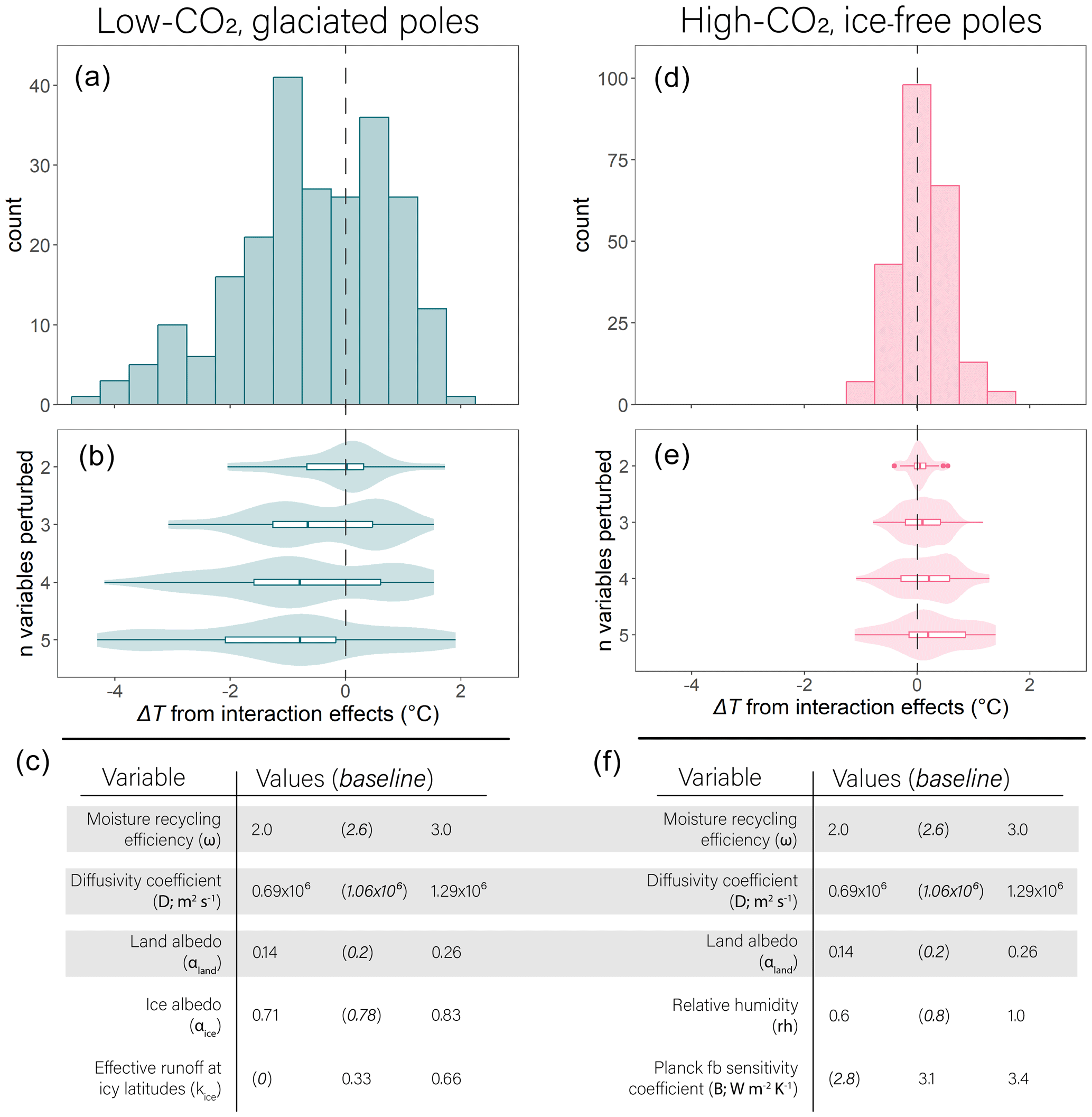
Figure 5 Factorial experiments show some non-linear interaction. (a) Histogram of deviation of global mean surface temperature from the expected temperature due to the sum of individual effects (ΔT) for the low-CO₂ case. A negative tail indicates larger interaction effects with more ice growth. (b) Density plots showing that the spread in the deviation from zero tends to increase as more variables are perturbed. (c) Table of variables and values (unperturbed in parentheses), with gray shading highlighting variables with the same values in the low- and high-CO₂ cases. Panels (d), (e), and (f) are the same as panels (a), (b), and (c), respectively, but for the high-CO₂ case where the globe remains ice-free in all simulations.

4.3 Factorial experiments and interaction effects

Factorial experiments demonstrate that interaction effects are prevalent in the model, especially under low-pCO₂, glacial conditions (Fig. 5). When perturbed, each variable that we tested (Fig. 5c, f) can alter the spatial pattern of temperature and/or runoff, thereby influencing the global weathering flux and the steady-state climate required to balance the carbon cycle $\left(\frac{\mathrm{d}{M}_C}{\mathrm{d}t}=\mathrm{0}\right)$. For the low-pCO₂ case, we include perturbations to ice albedo and k_ice, the fraction of runoff that contributes to weathering beneath an ice sheet, both of which have no effect when ice is absent. We substitute these variables for relative humidity and the Planck feedback sensitivity parameter in the high-CO₂ case. In many experiments, perturbing multiple variables at once yields a similar global temperature to the net effect of perturbing each variable independently. Still, interaction effects appear in the low- and high-pCO₂ cases, the magnitude of which increases as more variables are perturbed (Fig. 5b, e).

Notably, interaction effects in the low-pCO₂ case have a larger effect on global cooling than global warming, creating the negative tail in Fig. 5a. This effect is likely related to the positive, non-linear ice–albedo feedback which strengthens with cooling, potentially amplifying interaction effects. Further, the absence of an ice–albedo feedback is associated with weaker interaction effects in the high-pCO₂ case (Fig. 5d, e). A direct comparison of the low- and high-pCO₂ experiments in which the same variables are perturbed yields the same result: interaction effects are weaker without an ice–albedo feedback. Overall, our factorial experiments emphasize the complexity that emerges when positive feedbacks such an ice–albedo feedback play a role in long-term carbon cycling. Interactions between variables, especially in colder, icy climates, makes it difficult to disentangle any individual variable's effect.

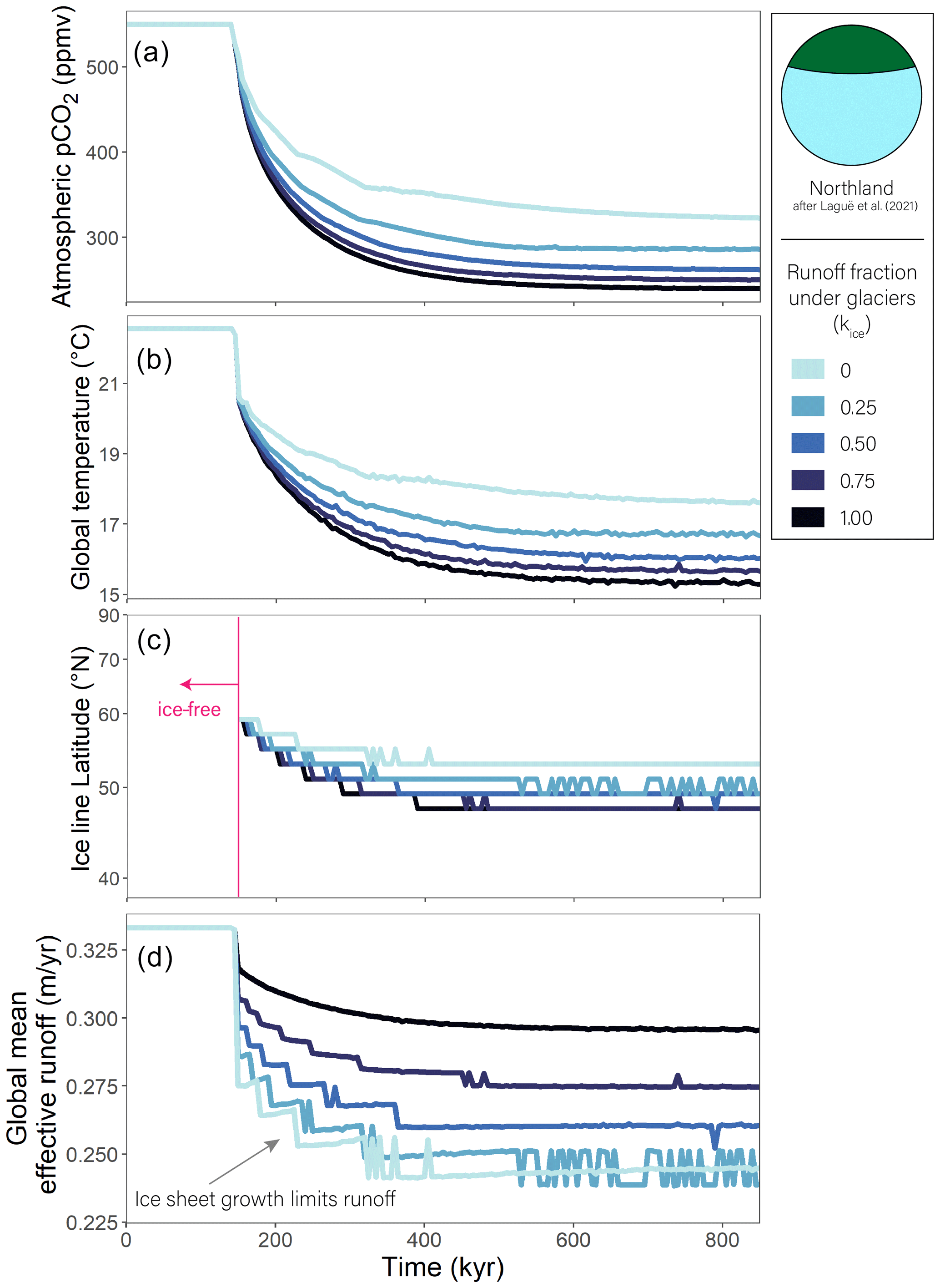
Figure 6 Effect of ice sheets inhibiting runoff. Temporal evolution of atmospheric pCO₂ (a), global mean temperature (b), the latitude of the ice line (note the y axis is an equal-area grid) (c), and global mean effective runoff (d) for different k_ice scenarios when the volcanic input is halved. Note that panel (d) refers to terrestrial runoff relevant for weathering (which accounts for changes k_ice). When k_ice at ice-covered latitudes is zero (light-blue line), a smaller change in temperature is needed to balance the carbon cycle. The largest change is necessary when k_ice is one and runoff is equal to the total runoff predicted by the MEBM (black line).

4.4 Varying the effect of ice cover on weathering

When we halve the volcanic flux of CO₂ in our model, allowing ice cover to increase, the temperature and pCO₂ of the new equilibrium climate state depend on k_ice (or how much ice cover decreases the effective runoff available to weather rock). With more effective runoff, weathering fluxes remain high at glaciated latitudes, requiring overall colder temperatures, more ice cover, and lower pCO₂ to balance the lower volcanic emissions flux (Fig. 6). The opposite is true for low k_ice. Here, runoff (and, thus, weathering) decreases more drastically with temperature and ice growth, requiring a smaller temperature decrease to balance the drop in volcanism. The effect of ice growth on runoff can be seen in Fig. 6d, where runoff decreases in a stepwise fashion, tracking spurts of ice sheet growth, when effective runoff is very low. The lowest k_ice simulation has a similar global mean runoff to the 0.25 case because of competing temperature effects. The warmer temperatures of the k_ice=0 case limit ice cover and lead to higher runoff in ice-free regions, partially counteracting the lower k_ice where ice exists. In short, when ice sheets are present, the global temperature response to volcanic CO₂ emissions depends strongly on how ice sheets impact weathering in our model, particularly when much of the global land mass exists at the poles. The more ice sheets inhibit weathering, the smaller the change in temperature required to balance a volcanic perturbation.

We note that changes in k_ice have no impact on climate or the long-term carbon cycle in an ice-free world (where k_ice=1 everywhere). This is why all simulations start at the same ice-free initial conditions in Fig. 6. As a result, these simulations can be directly compared because all terms that are defined when the model is initialized – including W_sil, which impacts the strength of the silicate weathering feedback separately from k_ice – are equal. If we initialized the model in a glaciated state, W_sil would have to vary with k_ice to maintain a balanced carbon cycle at the first time step, and our results would confound the direct effect of changing k_ice and the indirect effect of changes in W_sil.

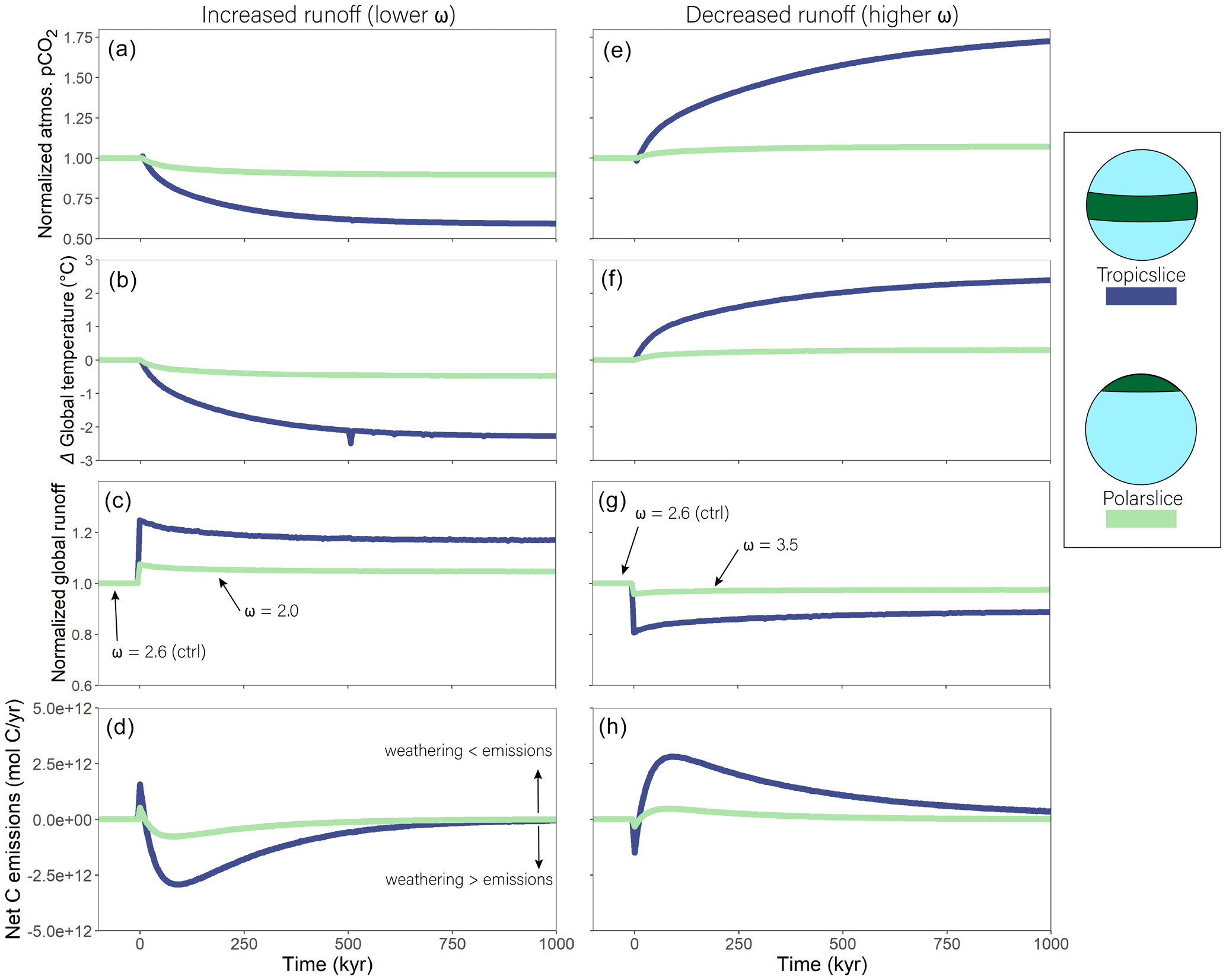
Figure 7 Abrupt change in evapotranspiration efficiency (ω). All changes are relative to each run's pre-perturbation value. Effect of instantaneous decrease in Budyko ω at time zero from 2.6 to 2.0 (a–d) on atmospheric pCO₂ (a), the change in global temperature (b), global runoff, and normalized (c) and net carbon emissions (d). Panels (e)–(h) show the same respective variables but for an increase in ω from 2.6 to 3.5. The larger-magnitude climate response of Tropicslice world compared with Polarslice world is owed to the larger-magnitude change in climate from the change in ω rather than changes in the strength of the silicate weathering feedback (see text).

4.5 Instantaneous change in moisture recycling efficiency

Figure 7 shows the model climate and carbon response to an abrupt increase (panels a, b, c, d) and decrease (panels e, f, g, h) in runoff, as determined by the recycling efficiency parameter ω. Results are shown as a factor change (panels a, c, e, g) or an anomaly (panels b, d, f, h) from pre-perturbation (time <0) because the different continental configurations cause somewhat different initial climate states, although the relative responses are robust. When ω decreases from 2.6 to 2.0, runoff increases everywhere, driving more weathering. Initially, the increase in weathering creates a “blip” in net C emissions (defined as the sum of fluxes in Eq. 23) because carbonate weathering becomes a transient source of carbon, compensated for by subsequent burial. In this section and the next, we ignore this transient blip when we note the effect of the climate variable on net C emissions.

The magnitude of the weathering (and, thus, climate) response to changing ω depends on geography. Runoff increases by a larger fraction in Tropicslice compared with Polarslice world because runoff is most sensitive to ω when precipitation over potential evapotranspiration is closer to one (see, e.g., Zhang et al., 2004, their Fig. 5), as is the case for Tropicslice world. This larger increase in relative runoff causes a larger fractional increase in weathering (decrease in net C emissions) in Tropicslice world (Fig. 7d), requiring relatively more cooling (Fig. 7b) to reach a new steady state in the carbon cycle with zero net emissions. The same relative response between Polarslice and Tropicslice world can be seen in the case where ω is increased, causing a decrease in runoff (Fig. 7e, f, g, h). In this case, the decrease in runoff is greater in Tropicslice world (Fig. 7g), leading to a larger increase in net C emissions as weathering declines (Fig. 7h).

In both cases (decreasing and increasing ω), Tropicslice world takes longer to return to zero net C emissions compared with Polarslice world, mostly because the runoff perturbation is relatively larger (Fig. 7c, g). We note that the runoff response to warming is similar in Polarslice and Tropicslice worlds, but silicate weathering is more responsive to global temperature in Polarslice world (Fig. S3). This effect is due to polar amplification of warming causing a greater increase in weathering per increase in global temperature (and runoff) in Polarslice world. The same effect can be seen in Fig. 4, where weathering responds strongly to warming in the Northern Hemisphere middle to high latitudes despite a relatively weak runoff response. Consequently, the weathering response to pCO₂ is different between the Polarslice and Tropicslice worlds, despite similar runoff responses to pCO₂ (Fig. S3).

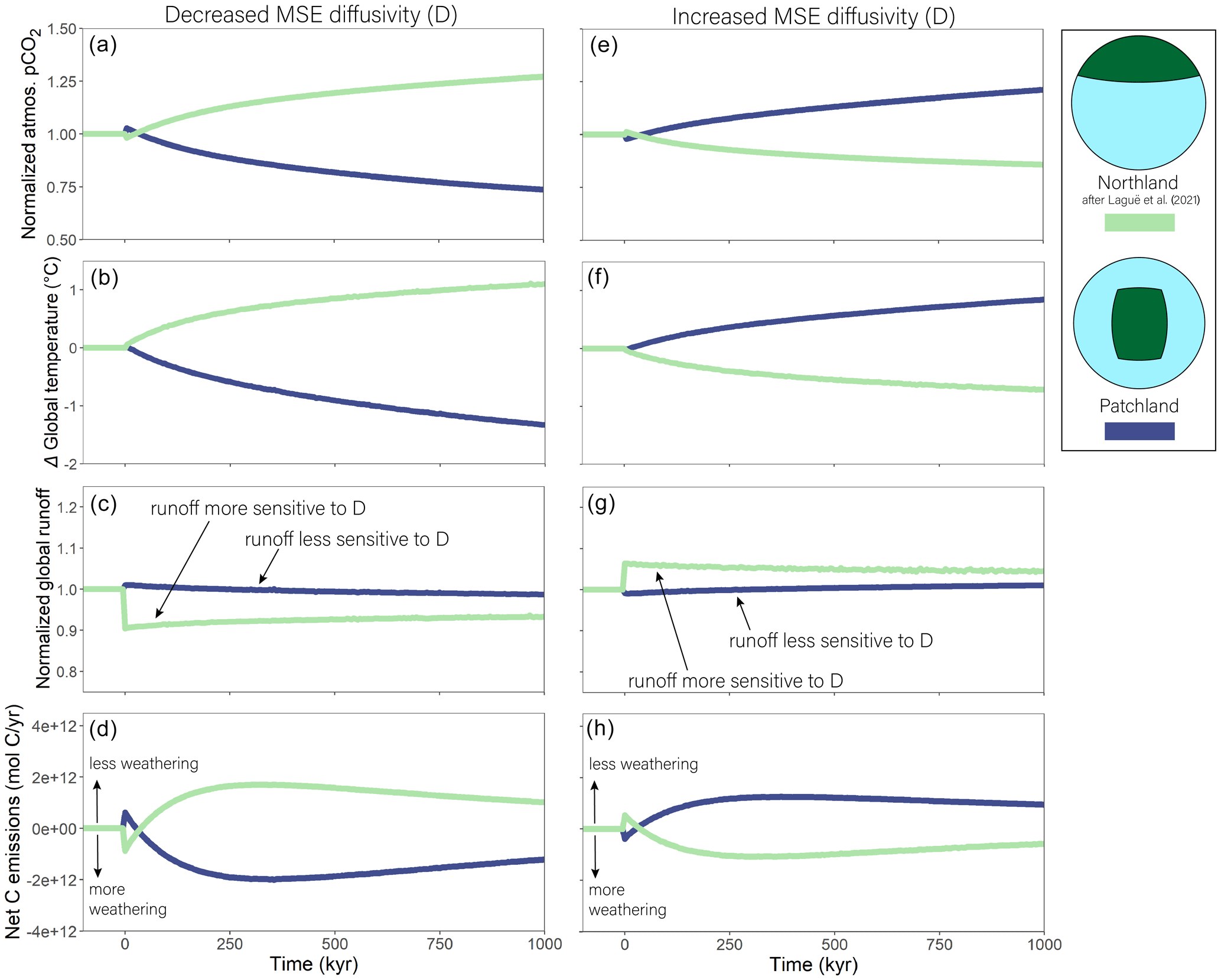
Figure 8 Abrupt change in moist static energy (MSE) diffusivity (D). All changes are relative to each run's pre-perturbation value. Effect of an instantaneous decrease in the diffusivity coefficient from 1.06×10⁶ to 0.71×10⁶ m² s⁻¹ at time zero on atmospheric pCO₂ (a), the change in global temperature (b), and the fractional change in global runoff (c) and net carbon emissions (d). Panels (e)–(h) show the same respective variables but for an increase in D to 1.41×10⁶ m² s⁻¹. Note that, unlike other variables, the runoff response is not symmetric between the geographies because runoff is sensitive to D in Northland world but much less sensitive in Patchland world. Simulations are ice-free at all times.

4.6 Instantaneous change in the diffusivity of moist static energy

In our model, moist static energy diffusivity (D) determines how efficiently the surplus of atmospheric energy in the tropics and subtropics (where incoming radiation exceeds outgoing radiation) is transported toward the polar regions where there is an atmospheric energy deficit (outgoing radiation exceeds incoming radiation). D has only a loose physical meaning, as it is convenient in models of this level of complexity to parameterize poleward moist static energy transport as a diffusive process to avert the complex underlying transport physics. Still, the D that produces the best MEBM fit to true climate data is generally thought to change with geography, pCO₂, and other factors (Frierson et al., 2006; Peterson and Boos, 2020; Siler et al., 2018). At present, we lack rigorous process-based formulations for the D response to climate and geography; nevertheless, we simulate its effect on long-term carbon cycling to build intuition for its role in the MEBM and broader CH2O-CHOO TRAIN framework.

The Patchland and Northland worlds show distinct responses to the same change in D (Fig. 8). A decrease in D lowers pCO₂ and cools Patchland world, whereas the same decrease in D raises pCO₂ and warms Northland world (Fig. 8a, b). The divergent climate responses are caused by diverging weathering responses which, in turn, are caused by spatially variable changes in runoff and continental temperature (Fig. S4). Weathering increases with lower D in Patchland mostly due to warming in the subtropics and tropics at the expense of cooling at higher latitudes. Runoff increases in the subtropics but decreases slightly in the tropics such that the effect of runoff on weathering is small. The fact that temperature, not runoff, drives the increase in weathering in Patchland world is evident in Fig. 8c. Here, the initial increase in runoff in Patchland world is small, and runoff continues to decrease with time as the planet cools. Conversely, runoff and temperature both drive the weathering response in Northland world. Runoff initially decreases in the polar continent as D decreases (Fig. 8c), and runoff then gradually increases as the planet warms and weathering begins to balance emissions. Increasing D leads to essentially the opposite effect (Fig. 8e, f, g, h). Patchland world warms due to an initial drop in weathering while Northland world cools due to an initial weathering increase. As in the case of decreasing D, the change in weathering in Patchland world is primarily driven by temperature – Patchland world runoff is less sensitive to D – whereas temperature and runoff increase in concert with increase weathering in Northland world. We note that the direct effect of changing D on global temperature is small. Changing D will warm some regions and cool others, with the opposing effects largely canceling out (especially when the poles are ice-free and there is no ice–albedo feedback). However, the terrestrial climate response to D – which can be sensitive to the continental geography – determines its effect on weathering and, therefore, long-term global temperature.

5 Model applications and their limitations

The primary feature of our model relative to existing long-term carbon cycle frameworks is the intermediate-complexity representation of climate via the MEBM. We expect that the most useful applications of the model will include those analyzing the sensitivity of long-term carbon cycle dynamics to various features of the complex climate system that are difficult to capture in simpler models and difficult to efficiently test or modify in more complex models. The ice–albedo feedback, the role of ice sheets in weathering, polar amplification of warming, and changes in moist static energy diffusivity – processes explored above – are examples of climate features that can impact long-term carbon cycling and can be easily investigated in the CH2O-CHOO TRAIN framework but are often difficult to efficiently manipulate in more complex models. Still, there are important limitations to such model applications that arise from the underlying model assumptions. We emphasize these limitations here while also highlighting some of the advantages that justify our use of the MEBM and its one-dimensional approach to represent climate.

5.1 Climate and weathering

A primary limitation of the CH2O-CHOO TRAIN framework is that the model must be tuned to the desired baseline climate and weathering state. Parameters such as the diffusivity coefficient; land, ocean, and ice albedo; climate sensitivity; and others will affect the climate state for a given pCO₂ and will determine the pCO₂ thresholds at which ice sheets initiate or collapse. Thus, if the model simulates a shift to an ice-free climate above 700 ppmv, this result should not be considered evidence that 700 ppmv represents a pCO₂ threshold for ice melt. Instead, we suggest that users first tune the model to match a desired baseline climate and its sensitivity (as informed by modern or geologic data, or climate model output). In this way, the model is perhaps most useful for studying how key aspects of climate affect the temporal evolution of long-term climate and carbon cycling, but it is less useful for constraining temperature and pCO₂ thresholds of climate transitions which are highly parameterized.

Baseline weathering fluxes in the model are also parameterized using a scaling coefficient to balance silicate weathering and volcanism at the first model time step. The weathering scaling coefficient, therefore, effectively modifies the strength of the silicate weathering feedback by assigning an implicit slope to the weathering–temperature relationship. The current version of our model also does not include explicitly parameterized seafloor basalt weathering (Coogan and Dosso, 2015). This flux is sensitive to deep water temperatures but not to runoff. As a consequence, for most simulations in which global temperature and runoff covary, the inclusion of seafloor weathering is not likely to fundamentally change the results presented here, but it will change the timescales over which the Earth system achieves a new stable equilibrium. However, in instances where runoff and temperature are negatively related or unrelated (this can occur in our model if all land exists at a latitude where runoff does not increase with warming), seafloor weathering may act to prevent a runaway greenhouse, although we note that this depends upon the sensitivity of seafloor basalt weathering to temperature.

The scaling coefficient for weathering is important to consider when comparing different geographic settings, volcanic fluxes, or climate states. Changing one of these factors (geography, volcanic flux, or climate) almost always changes another. For example, two different continental geographies with different runoff distributions will require one of the following: (1) two different scaling coefficients to match a given volcanic flux (thus maintaining a constant DIC residence time), (2) two different volcanic fluxes for a constant scaling coefficient, or (3) two different climate states for a constant scaling coefficient and volcanic flux. Importantly, this limitation is not unique to our model framework. In any model for the long-term carbon cycle, it is generally impossible to compare two different geographic configurations, volcanic fluxes, or climate states while also holding all else constant. Changing any of these terms will tend to put the carbon cycle out of balance, requiring compensation somewhere else. Due to this limitation, certain research questions must be approached with caution. For example, the question of whether one continental geography or another yields a stronger silicate weathering feedback is difficult to test because the weathering scaling coefficients, the volcanic fluxes of CO₂, and/or the baseline climate states must differ, all of which may also affect the feedback strength.

Hydrological fluxes, land albedo, and GPP are not coupled in our model, and precipitation does not affect land albedo nor GPP. A wetter climate is expected to decrease land surface albedo by supporting a greater leaf area and, therefore, a darker surface, whereas a drier climate tends to have the opposite effect (e.g., Charney, 1975; Claussen, 1997). Decoupling these processes in our model means that precipitation is not responsive to vegetation (i.e., no precipitation–vegetation albedo feedback) and the weathering response to hydrological fluxes is solely due to their effect on runoff, with no indirect additional effect via GPP (see Eq. 20) and soil pCO₂. Including such a parameterization would likely heighten the sensitivity of weathering to hydrologic change.

However, this formulation of climate and weathering in the model also offers distinct advantages. Perhaps the most important advantage is that weathering is not explicitly parameterized to increase with pCO₂, as is common with low-dimensional box models of the long-term carbon cycle (Bergman, 2004; Caves et al., 2016; Zeebe, 2012). In contrast, higher-order models use climate model data where the temperature and (especially) runoff response to pCO₂ is more complex and, in some cases, weathering has been shown to decrease with warming (Pollard et al., 2013). In our model formulation, the strength and direction of the weathering response to climate mostly depends on the boundary conditions which determine where continental runoff occurs and how it responds to pCO₂. Thus, similar to more complex two- and three-dimensional models, our one-dimensional framework allows for a dynamic silicate weathering feedback which responds to time-variant conditions such as ice cover (Fig. 6) and time-invariant conditions such as geography (Figs. 7, 8). As a result, it is easy to explore scenarios that cause or prevent a positive weathering feedback and runaway climate states in the CH2O-CHOO TRAIN framework.

Another advantage of our model framework lies in how ice sheets interact with climate and carbon cycling. While the exact role of ice sheets in the long-term carbon cycle remains unclear (e.g., von Blanckenburg et al., 2015; Torres et al., 2017), our model presents a framework to test existing hypotheses in such a way that ice, climate, and the long-term carbon cycle are fully coupled. This coupling to the long-term carbon cycle via weathering is generally absent in more complex, long-term models of ice sheet dynamics and climate (Pollard and DeConto, 2005; DeConto et al., 2008), although the ice–albedo feedback is not absent from all complex models with a long-term C-cycle component (Donnadieu et al., 2006; Holden et al., 2016; Ridgwell et al., 2007). Zero-dimensional box models have also been parameterized to account for icehouse–greenhouse transitions and their effect on weathering, with previous results showing climate oscillations as ice sheet growth and decay overshoots the equilibrium weathering flux (Zachos and Kump, 2005). Consistent with more complex models (Pollard et al., 2013), we were unable to replicate this effect in our one-dimensional framework, largely because polar weathering fluxes are only a small fraction of global weathering fluxes in most continental geographies.

5.2 The zonal-mean framework

The key assumption that distinguishes our model from previous one-dimensional energy balance climate models coupled to the long-term carbon cycle is that the zonal-mean climatology produced by the MEBM adequately represents terrestrial (hydro)climate conditions. Indeed, certain assumptions within the MEBM only hold over ocean. For example, we prescribe a spatially uniform relative humidity value of 80 %, consistent with oceanic, but not terrestrial, near-surface conditions. We note it is possible to prescribe a spatially variable humidity field, as done in previous work (Peterson and Boos, 2020). Further, the evaporation approximation used in the MEBM (Siler et al., 2018, 2019) is valid over oceans but not over land. This is due in part to the fact that evaporation is not limited by water availability, as is commonly the case over land. As mentioned previously, our approach to translate zonal-mean evaporation to terrestrial evapotranspiration involves imposing a water limitation constraint following the Budyko hydrologic balance framework – a step that provides physically reasonable evapotranspiration and runoff values but decouples terrestrial evapotranspiration from the zonal-mean climatology. While we make efforts to derive realistic terrestrial hydrologic budgets from the zonal-mean MEBM results, it is clear that the zonal-mean climatology cannot be considered equivalent to terrestrial climatology everywhere.

Another challenge is that the zonal fragmentation of land, not captured in the zonal-mean framework, can impact the relationship between zonal-mean climatology and terrestrial climatology. In our model, a supercontinent yields the same result as many small continents as long as the zonal-mean land distribution is the same. However, more fragmented land masses can lead to larger weathering fluxes, as supercontinents limit moisture delivery to continental interiors (Baum et al., 2022). Thus, our model implicitly assumes that less fragmented land serves as an adequate moisture source to maintain well-watered continental interiors (similar to the Amazon Basin today). This caveat is particularly relevant for our idealized geographies that span the planet zonally, discussed in the next section. In these cases, the model can provide useful insights to the coupled climate–carbon cycle but may give very different results from more complex two-dimensional models using the same continental configuration.

Deriving zonal-mean weathering rates from the zonal-mean climatology can present another challenge. Land surface reactivity can change over space at a given latitude depending on topography, soil age, and other factors (e.g., Maher and Chamberlain, 2014; Waldbauer and Chamberlain, 2005). A landscape with some given mean runoff, temperature, and reactivity will weather more if high runoff and high reactivity co-occur (as in a wet coastal mountain range with a dry inland plain). Meanwhile, the same zonal-mean runoff, temperature, and reactivity will lead to less weathering if high runoff occurs in a less reactive region (as in a wet coastal plain with a drier inland mountain range). While the covariation in temperature, runoff, and reactivity at a given latitude influences the zonal-mean weathering rate, this information is lost in our one-dimensional approach.

Still, the zonal-mean climatology and weathering remain useful features of our model, even if they are not perfect representations of how the two-dimensional landscape is projected into one-dimensional space. The zonal-mean approach is computationally efficient and makes it possible to consider how spatially complex changes in hydroclimate can impact weathering during a carbon cycle perturbation. For example, if ice melt in the North Pole causes the tropical rain belt (ITCZ) to shift north, the weathering response to this ice melt will depend in part on whether there is more or less land in the ITCZ's new location. The effect of this ITCZ shift would be lost in most zero-dimensional models where weathering and runoff are single functions of temperature or pCO₂. Similarly, changes in land albedo are known to shift tropical rainfall (e.g., Charney, 1975; Claussen, 1997) and can be efficiently represented in this zonal-mean framework to explore the carbon cycle consequences. In sum, the zonal-mean approach captures critical, realistic processes that lower-dimensional models usually omit while providing more computational efficiency compared with more complex models.

6 Next stops

The CH2O-CHOO TRAIN is designed to be computationally efficient and highly customizable, presenting opportunities for new features, processes, and complexity in future work. For example, terms such as humidity, the diffusivity coefficient, lithology, and rock reactivity are globally constant in the idealized simulations presented here but could easily be made spatially explicit in the current model framework. We also recognize room for improvement in certain aspects of the model. For example, our current ice sheet formulation is rather crude, with a prescribed ice sheet albedo that occurs whenever the temperature drops below a prescribed threshold. More sophisticated ice sheet parameterizations in MEBMs have accounted for other effects such as ice thickness, sea ice thermodynamics, and seasonal ice formation and retreat (Feldl and Merlis, 2021). The effect of seasonal insolation, specifically, is a feature of interest for simulating tropical weathering where changes in past rainfall often track seasonal insolation trends. Adding insolation seasonality and more complex ice sheet dynamics would undoubtedly increase the computational expense of the model.

The zonal-mean framework of our model is also well-suited for simulating the effect of spatially variable radiative feedbacks on the climate response to carbon cycle perturbations. While the ice–albedo feedback is already accounted for via a temperature dependency of albedo, other feedbacks such as cloud feedbacks are currently absent from the model. However, the zonal pattern of such feedbacks could easily be prescribed, perhaps from climate model output, to explore how the effect of these feedbacks on temperature and hydroclimate impact the temporal evolution of weathering (Roe et al., 2015). Still, the suite of feedbacks in the current model, including the combination of radiative and weathering feedbacks, are rarely considered in a single model framework. Therefore, the CH2O-CHOO TRAIN provides opportunities to explore the complexity that emerges through the myriad interactions between climate and the long-term carbon cycle in the geologic past.