the Creative Commons Attribution 4.0 License.
the Creative Commons Attribution 4.0 License.
 | 22 Sep 2023
Enhancing the representation of water management in global hydrological models
Guta Wakbulcho Abeshu
Fuqiang Tian
Thomas Wild
Mengqi Zhao
Sean Turner
A. F. M. Kamal Chowdhury
Chris R. Vernon
Hongchang Hu
Yuan Zhuang
Mohamad Hejazi
This study enhances an existing global hydrological model (GHM), Xanthos, by adding a new water management module that distinguishes between the operational characteristics of irrigation, hydropower, and flood control reservoirs. We remapped reservoirs in the Global Reservoir and Dam (GRanD) database to the 0.5∘ spatial resolution in Xanthos so that a single lumped reservoir exists per grid cell, which yielded 3790 large reservoirs. We implemented unique operation rules for each reservoir type, based on their primary purposes. In particular, hydropower reservoirs have been treated as flood control reservoirs in previous GHM studies, while here, we determined the operation rules for hydropower reservoirs via optimization that maximizes long-term hydropower production. We conducted global simulations using the enhanced Xanthos and validated monthly streamflow for 91 large river basins, where high-quality observed streamflow data were available. A total of 1878 (296 hydropower, 486 irrigation, and 1096 flood control and others) out of the 3790 reservoirs are located in the 91 basins and are part of our reported results. The Kling–Gupta efficiency (KGE) value (after adding the new water management) is ≥ 0.5 and ≥ 0.0 in 39 and 81 basins, respectively. After adding the new water management module, model performance improved for 75 out of 91 basins and worsened for only 7. To measure the relative difference between explicitly representing hydropower reservoirs and representing hydropower reservoirs as flood control reservoirs (as is commonly done in other GHMs), we use the normalized root mean square error (NRMSE) and the coefficient of determination (R2). Out of the 296 hydropower reservoirs, the NRMSE is > 0.25 (i.e., considering 0.25 to represent a moderate difference) for over 44 % of the 296 reservoirs when comparing both the simulated reservoir releases and storage time series between the two simulations. We suggest that correctly representing hydropower reservoirs in GHMs could have important implications for our understanding and management of freshwater resource challenges at regional-to-global scales. This enhanced global water management modeling framework will allow the analysis of future global reservoir development and management from a coupled human–earth system perspective.
- Article
(7409 KB) - Full-text XML
-
Supplement
(2062 KB) - BibTeX
- EndNote


Reservoirs are pivotal in fulfilling various societal needs, including irrigation, hydropower production, flood control, domestic water supply, and navigation, to list a few (Belletti et al., 2020; Biemans et al., 2011; Grill et al., 2019). There are 6862 large reservoirs (≥ 0.1 km3) globally, with a cumulative storage capacity of 6197 km3 in the Global Reservoir and Dam (GRanD) dataset (Lehner et al., 2011). Many of these reservoirs serve multiple purposes. However, if we partition reservoirs into categories based on their primary purposes, 1789 are irrigation reservoirs, with a total storage capacity of ∼ 1100 km3; 1541 are hydropower reservoirs, with a total storage capacity of ∼ 3880 km3; 542 are flood control reservoirs, with a total storage capacity of ∼ 509 km3; and the rest are water supply, navigation, or recreation reservoirs. Water storage and release in any given reservoir are managed, based on the reservoir's purposes. It is, therefore, important in global hydrological models (GHMs) to represent how management strategies differ across reservoirs with different purposes in order to more accurately simulate water balances and explore the implications of alternative water management strategies. It is particularly important to distinguish the behavior of hydropower reservoirs from others because hydropower production represents the primary purpose for nearly 63 % (based on GRanD) of the total global reservoir storage capacity.
Hanasaki et al. (2006) proposed a generic reservoir simulation scheme for use in GHMs that has been widely used (denoted hereinafter as the Hanasaki scheme). This scheme categorizes all reservoirs into only two types, based on their primary purposes, namely irrigation and non-irrigation reservoirs. All non-irrigation reservoirs are essentially simulated as flood control reservoirs. The Hanasaki scheme determines reservoir release in two stages. First, the provisional release is estimated. For irrigation reservoirs, the provisional release is estimated as a function of the demand for water placed on the reservoir, while provisional release from non-irrigation reservoirs is the long-term mean inflow. The provisional release is then adjusted based on the reservoir's degree of regulation (i.e., the ratio of reservoir storage capacity to inflow).
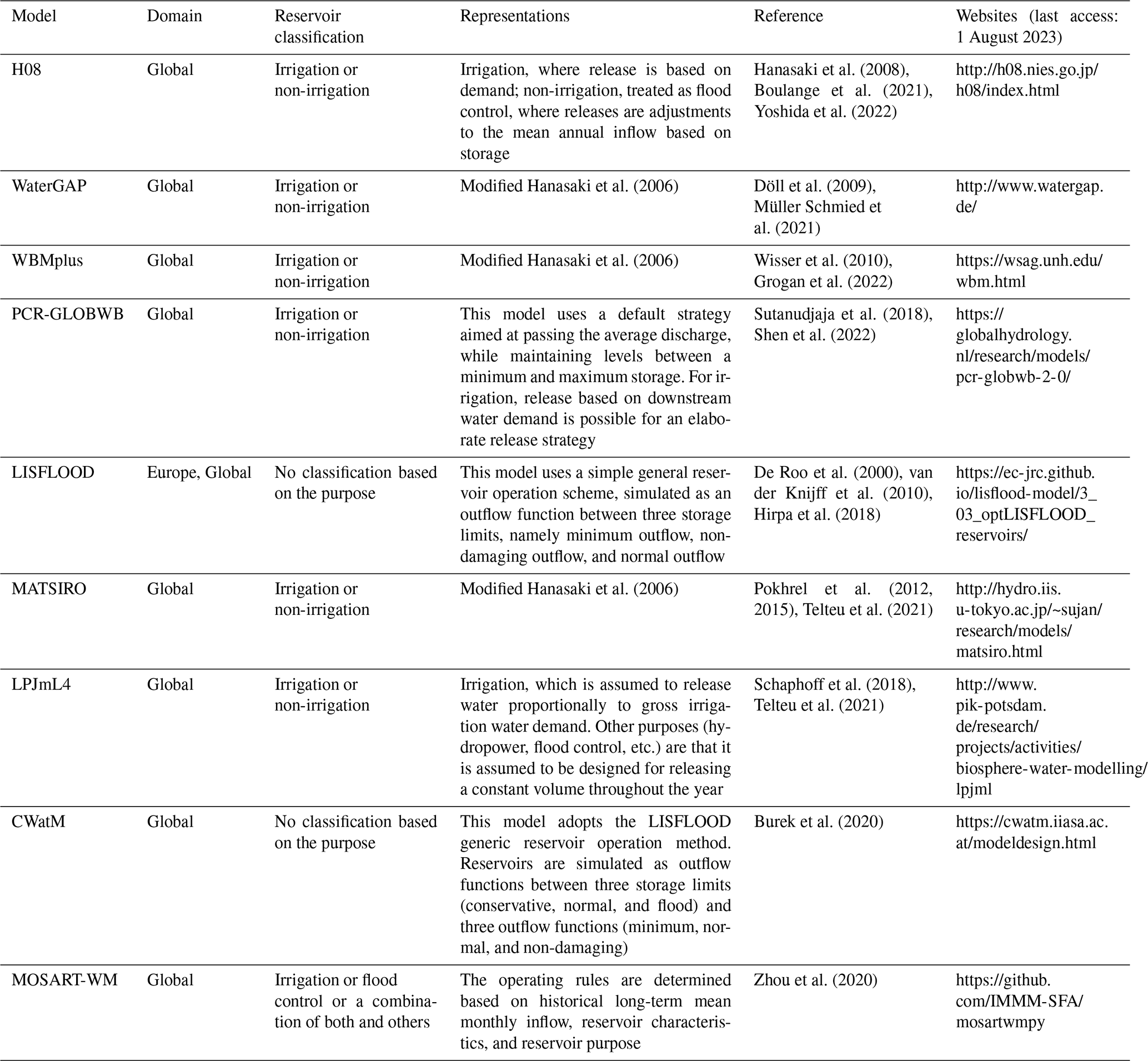
Most existing GHMs (see Table 1) adopt the Hanasaki classification and treat reservoirs as irrigation or non-irrigation (Burek et al., 2020; Hanasaki et al., 2008; Pokhrel et al., 2012; Schaphoff et al., 2018; Müller Schmied et al., 2021; Sutanudjaja et al., 2018; van der Knijff et al., 2010; Wisser et al., 2010; Zhou et al., 2020). Several GHM studies have employed this scheme with some modifications, including H08 (Hanasaki et al., 2008), MATSIRO-TRIP (Pokhrel et al., 2012), WaterGAP2 (Müller Schmied et al., 2021), WBMplus (Wisser et al., 2010), and LPJmL4 (Schaphoff et al., 2018). For example, some studies have modified the technique for estimating the parameters for irrigation reservoirs (i.e., water demand and spatial extent of the dependent area of a specific reservoir; Biemans et al., 2011). LPJmL4 (Schaphoff et al., 2018) and PCR-GLOBWB (Sutanudjaja et al., 2018) estimate irrigation reservoir release based on water demand, and for all other primary purposes, these models use a default strategy, where they release a pre-determined value (e.g., average discharge) while maintaining levels between a minimum and maximum storage. LISFLOOD (van der Knijff et al., 2010) and CWatM (Burek et al., 2020) do not classify reservoirs based on their purposes. Instead, they use three pre-determined releases based on storage, namely minimum outflow, non-damaging outflow, and normal outflow.
Table 1List of global hydrological models with reservoir representations. The domain column indicates the spatial scale at which the model has been applied. The representations column describes how each reservoir class (from the reservoir classification column) is simulated. In all cases, the reservoirs are integrated into the models. The reservoir classification column shows how the reservoirs were represented.
Most GHMs, however, still largely follow the Hanasaki scheme in treating all non-irrigation reservoirs as flood control reservoirs. In the Hanasaki scheme, the inflow, minimum pool level, maximum static full level, and water stored at the beginning of the hydrological year are the only significant factors controlling the magnitude and timing of water release (Hanasaki et al., 2006; Yassin et al., 2019). In reality, among non-irrigation reservoirs, hydropower reservoirs are typically operated differently from flood control reservoirs (Turner et al., 2017; Loucks et al., 2017). An essential difference between them is that hydropower reservoirs mostly operate with the objective of storing water over certain target levels to maximize releases through turbines (Loucks et al., 2017). The minimum and maximum releases corresponding to the minimum and maximum storage levels are also pre-determined. Furthermore, in large storage hydropower reservoirs with a large degree of regulation, storage levels may vary significantly over the course of a year (between the minimum and maximum storage levels) to avoid significant spillage and enable reliable hydropower generation throughout the year. Conversely, an essential feature of flood control reservoirs is to provide a reliable capacity to retain a predicted or unforeseen future flooding event by emptying existing reservoir storage. The objective of flood control reservoirs is to reduce peak flow magnitude, and the storage level is only a concern when there is an incoming flood event (Votruba and Broza, 1989). Therefore, treating hydropower reservoirs as flood control reservoirs can significantly underestimate their operational benefits (Turner et al., 2017; Loucks et al., 2017).
The model performance implications of representing reservoirs as flood control versus hydropower reservoirs are evident at the individual reservoir level. However, there remains a gap in the literature regarding the regional-to-global model performance implications of the representation of hydropower reservoirs, given that GHMs are designed for applications at this spatial scale but have not yet explored this question surrounding the representation of hydropower (Best et al., 2011; Döll et al., 2009; Hanasaki et al., 2008; Pokhrel et al., 2012; Schaphoff et al., 2018; Wisser et al., 2010; Voisin et al., 2013). This study overcomes the aforementioned limitation by demonstrating an enhancement to how water management is employed in Xanthos, a global hydrological model. Xanthos is a relatively lightweight model designed to interact with the components of the Global Change Intersectoral Modeling System (GCIMS), which includes the Global Change Analysis Model (GCAM; Hejazi et al., 2013, 2014; Li et al., 2017) at its core, along with a broader suite of interacting energy, water, and land models. GCAM is an integrated tool for exploring the multisector dynamics of coupled human–earth systems and the response of these systems to global changes (Calvin et al., 2019). Aided by Xanthos, GCAM enables an internally consistent evaluation of time-evolving water supply (i.e., surface water, groundwater, and desalinated water) and demand dynamics across multiple sectors. As such, GCAM and Xanthos have been used in combination to study issues such as the relative contributions of humans and climate change to future global water scarcity (Graham et al., 2020), regional water scarcity (Birnbaum et al., 2022), and sub-national water scarcity (Khan et al., 2020; Wild et al., 2021b, c), as well as climate impacts on the future evolution of hydropower and the broader power sector (Arango-Aramburo et al., 2019; Santos da Silva et al., 2021). Nevertheless, the existing version of Xanthos, denoted here as Xanthos-original, focuses only on representing the natural global water balance without human interventions such as reservoirs (Hejazi et al., 2013; Liu et al., 2018; Vernon et al., 2019). Accounting for water management in the way we propose will ensure that the crucial role of reservoirs is represented in regulating streamflow by mediating water availability and demand (Wan et al., 2018, 2017; Zhang et al., 2020, 2019, 2018).
The specific objectives of this study are 3-fold: (1) to enhance Xanthos by adding a new water management module, where irrigation, hydropower, and flood control reservoirs are treated differently (this enhanced Xanthos is denoted as Xanthos-enhanced); (2) to evaluate the performance of Xanthos-enhanced in terms of reproducing observed streamflow variability; and (3) to understand the impacts of differentiating between flood control and hydropower reservoir operations on regional-to-global-scale water balance. The first two objectives represent improvements to Xanthos and, thus, potential improvements to a broad array of coupled human–earth system studies that rely on linkages between GCAM and Xanthos. The third objective has the potential to inform future improvements to a diverse array of GHMs (see Table 1) because our study is the first, to our knowledge, to explore the GHM performance improvements that can be gained by treating the operational characteristics of hydropower dams as distinct from those of irrigation and flood control dams.
Xanthos is a distributed global hydrological model with a spatial resolution of 0.5∘. Xanthos is a framework that enables users to create customized configurations of potential evapotranspiration estimation, runoff generation and concentration, routing, and post-processing modules (https://github.com/JGCRI/xanthos, last access: 1 August 2022). By accounting for reservoir operation and local water withdrawal, Xanthos-enhanced enables exploring the influence of water management (Fig. 1). This section focuses on the water management module but first briefly summarizes the runoff and river-routing components for completeness. For more details on the runoff and river-routing components, please refer to Li et al. (2017), Liu et al. (2018), and Vernon et al. (2019).
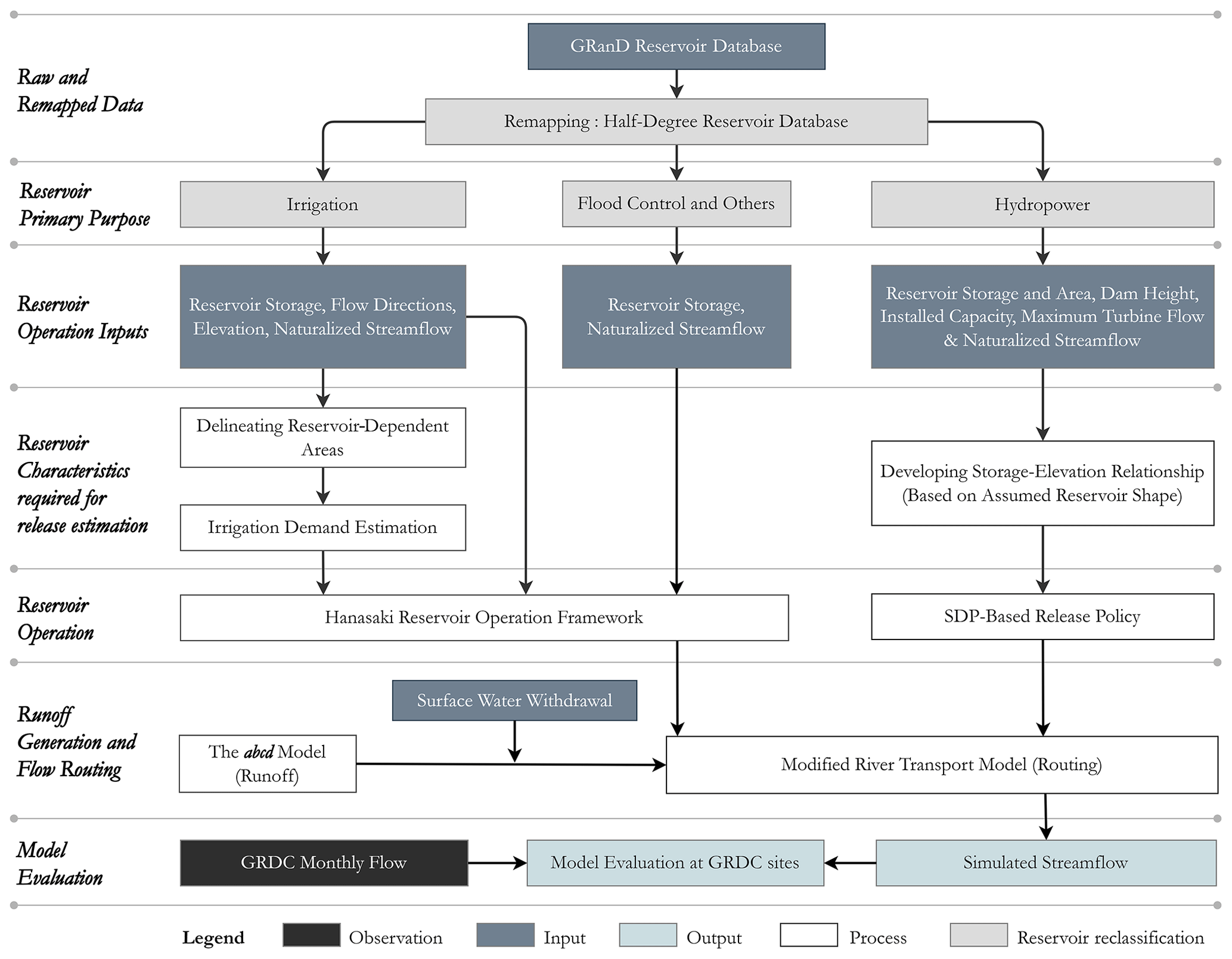
Figure 1A detailed schematic of the river-routing and reservoir management module in Xanthos-enhanced.
2.1 Runoff-generation module
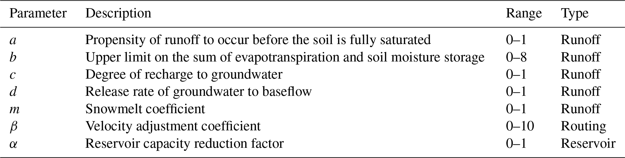
Runoff generation in Xanthos-original is based on the abcd model. First developed by Thomas (1981), abcd is a simple water balance model effective for capturing key hydrologic processes, and their interactions, in diverse climatic and landscape settings (Martinez and Gupta, 2010, 2011). Liu et al. (2018) introduced the abcd model into Xanthos as its runoff module for simulating direct runoff, baseflow, evapotranspiration, and soil moisture at a monthly time step. The sum of direct runoff and baseflow is denoted as total runoff, which feeds into the river-routing module. The five parameters in the abcd model are described in Table 2. Parameters a and b pertain to runoff characteristics, while c and d relate to shallow soil moisture and deeper groundwater storage. The fifth parameter is a snowmelt coefficient, denoted as m. Since Xanthos-original is a distributed model, each grid cell has its own set of abcd parameters, though these parameters can optionally have the same values for all grid cells within a given river basin. Xanthos classifies the global water system into 235 large water basins.
Table 2List of model parameters, description, and ranges. The parameters a, c, d, m, β, and α are dimensionless, and the unit for parameter b is meters. The value of α is fixed at 0.85, following Hanasaki et al. (2006).
2.2 River-routing module
In Xanthos, the routing of water through river networks is simulated using a simple cell-to-cell river-routing scheme, a modified version of the river transport model (Branstetter and Erickson, 2003) and hereinafter denoted as MRTM. MRTM is essentially based on the linear reservoir-routing method. The channel flow rate is estimated as a function of channel water storage, channel velocity, and flow distance from one grid cell to another (Zhou et al., 2015). MRTM uses spatially variable but temporally constant channel velocities, which were derived by averaging the long-term channel velocity simulations from Li et al. (2015). The flow distance values were derived by tracing the natural dominant river channel between grid cells to account for the meandering nature of rivers (Wu et al., 2011). Here we add a channel velocity adjustment coefficient (Table 2) to account for the uncertainties in our channel velocity field. For more details about MRTM, please refer to Zhou et al. (2015).
2.3 Water management module
To enhance Xanthos, we add a water management module on top of the river-routing module. The water management module represents the two most common surface water management activities of local surface water extraction and reservoir operation. Local surface water extraction is water that is locally consumed within a particular grid cell. For example, some fraction of the water applied to irrigated agricultural land may evaporate and effectively become unavailable for use in a given grid cell. This local consumptive water use is subtracted from the total runoff produced by the abcd model. The remaining runoff is discharged into the channels and routed downstream using MRTM. If the consumptive water use is greater than the total runoff in a grid cell, then the remaining runoff is zero. In such a case, the grid cell is considered to have unmet water demand or access to supply from other external sources, such as desalination or groundwater pumping, which are not currently represented in Xanthos. If there is a reservoir in a grid cell, then local runoff (after removing water consumption) and upstream inflow are first intercepted and stored in the reservoir. Reservoir operation is then invoked to estimate the release from the reservoir to the downstream grid cells. Note that a grid cell can contain only one reservoir. That is, if there are multiple individual reservoirs co-located in the same grid cell, we first lump these individual reservoirs into a single reservoir with a storage capacity equivalent to all the combined reservoirs. The primary purpose of this lumped reservoir within a given grid cell is determined in the following two steps: (1) sum up the storage capacities of the individual reservoirs in four categories based on their primary purposes (irrigation, hydropower, flood control, and other); and (2) in each category, sum up the reservoir storage capacities. The aggregated reservoir's primary purpose is assigned to the category with the largest summed storage capacity, while the volume of the single lumped reservoir is equivalent to the sum of all individual reservoir storage capacities across all purposes. The reservoir operation rule is defined for each lumped reservoir based on its primary purpose. For reservoir purposes, if the estimated release is unavailable or less than 10 % of the mean annual inflow, then the monthly release is set to the minimum environmental flow requirement (i.e., 10 % of the mean annual inflow; Tennant, 1976; Hanasaki et al., 2008; Müller Schmied et al., 2021). Next, we provide more details on the operating rule for each reservoir type (Fig. 1).
2.3.1 Irrigation reservoirs
Irrigation reservoirs are represented by adapting the widely adopted Hanasaki et al. (2006) approach, which determines the reservoir release based on the upstream inflow and the total water demand from the downstream areas. More specifically, for each irrigation reservoir, the provisional release is given as
where is the provisional monthly reservoir release (m3 s−1) in month m and year y; dm,y is the monthly mean total water demand from the downstream areas that are dependent on this reservoir (m3 s−1); dmean is the long-term mean monthly water demand from the downstream areas (m3 s−1); and imean is the mean annual inflow from upstream (m3 s−1). Both the magnitude of long-term average water demands and the monthly timing of demands are used as inputs, so releases are responsive to the timing of typical demands. The Hanasaki scheme has an allocation coefficient, which is a coefficient for grid cells with more than one reservoir upstream, but here it is assumed to be one and is thus not shown in Eq. (1). This is because, in this study, the dependent areas of reservoirs on the same stream do not overlap.
Though deterministic by nature, the provisional release equation for irrigation reservoirs is demand-driven. dm,y is calculated based on the delineated downstream-dependent grid cells. If dmean is greater than or equal to 50 % of the mean annual inflow imean, then 50 % of imean is continually released as a baseline, while seasonal release dynamics are determined by the ratio of monthly demand to dmean. If dmean is less than 50 % of imean, then the provisional release can be estimated as the mean annual inflow modified by the seasonal demand variation around the mean annual demand.
The provisional release is further adjusted based on the degree of regulation (γ), initial storage at the beginning of yth operational year (Sfirst,y), and reservoir capacity reduction factor (α). The degree of regulation is the ratio of reservoir storage capacity (C) to the annual total inflow in cubic meters per year (Imean). The reservoir capacity reduction factor is a non-dimensional constant that reduces the total reservoir capacity reported in GRanD to account for surcharge storage and storage reduction due to sediment accumulation. It ranges between 0–1, where a lower value means the reservoir capacity may have been significantly reduced by sediment accumulation, and at 0, the reservoir is not operational. The final release is estimated as follows:
where Rm,y is the monthly release (m3 s−1); im,y is the monthly inflow (m3 s−1); and Imean is the annual inflow (m3 yr−1).
The GRanD reservoirs can be classified into relatively large and small storage reservoirs, based on the degree of regulation. If a reservoir's total storage capacity is less than 50 % of its mean annual inflow, then it is considered a hydrologically small reservoir, whereas greater than 50 % indicates a hydrologically large reservoir. In relatively large reservoirs (upper part of Eq. 2), releases are relatively independent of their monthly inflows, while in relatively small reservoirs (lower part of Eq. 2), releases are dependent on their monthly inflows (Hanasaki et al., 2006).
The total water demand for each reservoir is estimated by summing up the water demand values from grid cells within the reservoir's downstream-dependent area. The reservoir-dependent area is determined, following Hanasaki et al. (2006), Haddeland et al. (2006), and Biemans et al. (2011). Specifically, the downstream spatial extent of reservoir dependency along the main stem is determined based on an average stream velocity and the study's temporal interval (monthly). Assuming an average velocity of 0.5 m s−1, the total travel distance of water in 1 month is 0.5 m s−1 × (30 × 24 × 3600 s per month) × (0.001 km m−1) = 1296 km per month. Therefore, the dependent downstream grid cells along the main stem are roughly 20 grid cells (0.5 × 0.5∘; about 55 km along each direction) downstream. If other reservoirs are located within this travel distance, then we assume that the dependency on the current reservoir stops and is taken over by the other reservoir (the allocation coefficient in Hanasaki et al. (2006) is set to one for this reason). We then delineate a buffer zone within ranges of four grid cells from each side of the main stem. Finally, assuming water movement is by gravity only, those grid cells with a mean elevation that is lower than that of the reservoir are identified as the reservoir's dependent grid cells within the buffer zone.
2.3.2 Hydropower reservoirs
We represent the operation of hydropower reservoirs using a stochastic dynamic programming (SDP) approach (Loucks et al., 2017; Turner et al., 2017). The SDP approach extends the dynamic programming approach to account for the uncertain nature of reservoir inflows explicitly (Loucks et al., 2017). It executes sequential decisions for temporal stages with nonlinear objectives, while considering reservoir inflows as random variables (Loucks et al., 2017). For a known inflow im,y and hydrologic state variables in the current period (Stedinger et al., 1984), the SDP formulation estimates the benefit function fm,y, resulting from each release decision Rm,y as
where T is the current system period (T=12 for a monthly operating scheme). The reservoir state at each decision-making time step, i.e., month m in the year y, is described by the storage Sm,y and the current inflow im,y. For each state and time step, the release decision Rm,y is selected to maximize the immediate benefit plus future benefit function , which depends on the resultant state of the system at time step m+1, i.e., the succeeding month.
The method for simulating the hydropower reservoir operation is adopted from “reservoir”, an R package that contains several reservoir release decision-making tools, including the SDP techniques described above (Turner, 2016). The same method was also employed in a global-scale study of hydroelectric plants' vulnerability to climate change (Turner et al., 2017). We integrated the SDP approach from this package (Turner, 2016; Turner et al., 2017) into Xanthos for hydropower release simulation. Here the SDP approach is first trained using the naturalized inflow to each reservoir to represent hydrological uncertainty, which we obtain by running MRTM without the water management option. The objective function is set to maximize hydropower production over the long term. The SDP procedure is executed to develop an energy-maximizing release policy for each month as a function of storage levels (see Fig. 1).
The working concept for the SDP algorithm we implemented is summarized as follows. Power (P in kilowatts) generated by a hydropower plant is given by , where ρg is the specific weight of water (kN m−3), R is turbine flow (m3 s−1), H is the turbine head (m), and η is efficiency (a constant value of 0.9 is used in this study). ρg term is a constant term and hence the power-generation variability is a function of R⋅H. Thus, maximizing the R⋅H translates to maximizing power production. The following four steps are used to identify an optimal policy (i.e., a hydropower-maximizing policy) from a given reservoir inflow realization. First, we discretize the maximum turbine flow (i.e., the maximum allowable flow rate through the turbine) into 10 increments (i.e., between 0 to maximum turbine flow) and the storage capacity into 1000 (i.e., between 0 to storage capacity) increments. Discretization of decision and state variable space is a common practice in implementing dynamic programming-based methods (Piccardi and Soncini-Sessa, 1991; Zeng et al., 2019). Second, we developed a depth–volume relationship, based on an assumed reservoir shape. Here we assume a wedge reservoir shape for all reservoirs globally in the absence of any global datasets to support more heterogeneous representations. The storage–volume relationship is employed to estimate storage depth (y) corresponding to 1000 discretized storage volume levels. The turbine head at each storage level was obtained from the sum of y and intake elevation. The intake elevation is computed as the maximum turbine head (i.e., the difference between reservoir pool level and turbine elevation) minus the maximum storage depth (equal to dam height in this study). Using the power equation, the maximum turbine head is computed from the plant-installed capacity and maximum turbine flow. Third, we have an array of releases and turbine heads from the discretization; multiplying them as a matrix yields a 1000×10 matrix of RH (i.e., 10 possible RH values for each storage level). In the present study, we select the policy that maximizes power generation. The best policy for each month (i.e., January to December) at all 1000 storage levels is obtained through backward recursive iterations (i.e., from December to January); this yields what we call the release policy, with a matrix with a size of 1000 (storage levels) ×12 (months). Last, during streamflow simulation, the storage volume and month are used to look up the optimal release policy table (i.e., the 1000×12 table), and the corresponding optimal release is determined. When a storage level is at the reservoir's maximum storage capacity, the release equals the maximum turbine flow that generates power at the power plant's installed capacity.
While the online integration of SDP with hydrological models brings considerable advantages, it also presents certain challenges. One such challenge is managing the uncertainties in the inflow data, as these directly influence the reservoir's operational policy. The effects of inflow uncertainty can lead to potential operational deviations, such as preemptive release of water due to overestimated inflows or undue conservation based on underestimated inflows. To lighten this challenge, a careful parameter selection process is implemented (see Sect. 2.4). The initial stage of this process prioritizes achieving a reliable long-term water balance that aligns closely with observations. By focusing on this balance, we aim to minimize the uncertainties inherent in the inflow data, thereby improving the reliability of operational decisions derived from the SDP model.
2.3.3 Flood control and other purpose reservoirs
The primary purpose of flood control reservoirs is to redistribute the floodwater from a flood season to a non-flood season. The operation of flood control reservoirs is also estimated, following Hanasaki et al. (2006).
where Rm,y is the monthly release (m3 s−1); and im,y is the monthly inflow (m3 s−1). In this study, release from reservoirs categorized as “others” is also determined as a function of inflow and storage characteristics only and is thus similar to flood control reservoirs. The logical reasoning for the equations employed here is in line with Eq. (2). For instance, as with irrigation reservoirs, the α and γ parameters are used to adjust the behavior of flood control reservoirs.
2.4 Model parameter determination strategy
In total, Xanthos-enhanced now includes seven parameters for the runoff and routing or water management modules. Typically, there are two strategies for determining the parameter values in a hydrologic model, namely calibration and estimation a priori (i.e., without calibration; Beven, 2012). Parameter calibration requires thousands of model runs and is only feasible for computationally inexpensive models. Feasibility can be compromised by parameter calibration efforts that require refactoring a model to run more efficiently, the budget required to scale simulations via high-performance computing resources, and the time needed for a comprehensive run. Furthermore, most hydrological models are subject to concerns surrounding equifinality, since the number of parameters, in most cases, far exceeds the number of observational variables available for calibration (Beven, 2006). Alternatively, parameter estimation a priori requires each parameter to be physically meaningful and have robust relationships with the existing climate or landscape information. These relationships are usually not readily available and have to be identified via sound prior knowledge (e.g., Li et al., 2015) or machine learning techniques (e.g., Abeshu et al., 2022; Li et al., 2021).
This study proposes a new, two-stage parameter determination strategy (described in Fig. 2) that seeks to overcome existing limitations by (1) screening out parameter sets that are not physically meaningful and (2) significantly reducing the overall computational burden associated with identifying optimal parameter sets. We seek to determine seven Xanthos parameters in total, namely five from the runoff module and two from the routing module, including water management. We determine runoff parameters in the first stage and routing parameters in the second stage. The runoff module runs separately from the routing and water management modules and is relatively lightweight, taking a standard personal computer less than 2 h to execute it at a global scale for one million simulations covering a 20-year duration. Meanwhile, the routing and water management modules are much more computationally intensive because they run at a 3 h time step to ensure numerical stability (Li et al., 2011, 2015). The first stage takes advantage of the lightweight runoff module to exhaustively explore the runoff parameter space before handing off favorable subsets of parameters to the second stage, which then limits its focus to the more computationally intensive search for the remaining two (routing) parameters. We describe the parameterization strategy in detail in the remainder of this section, whereas the results of implementing the strategy using a particular set of global data are detailed in Sect. 3.2. This strategy is designed based on the characteristics of the Xanthos modules, but we suggest that it has the potential to be useful in diverse global hydrological modeling contexts.
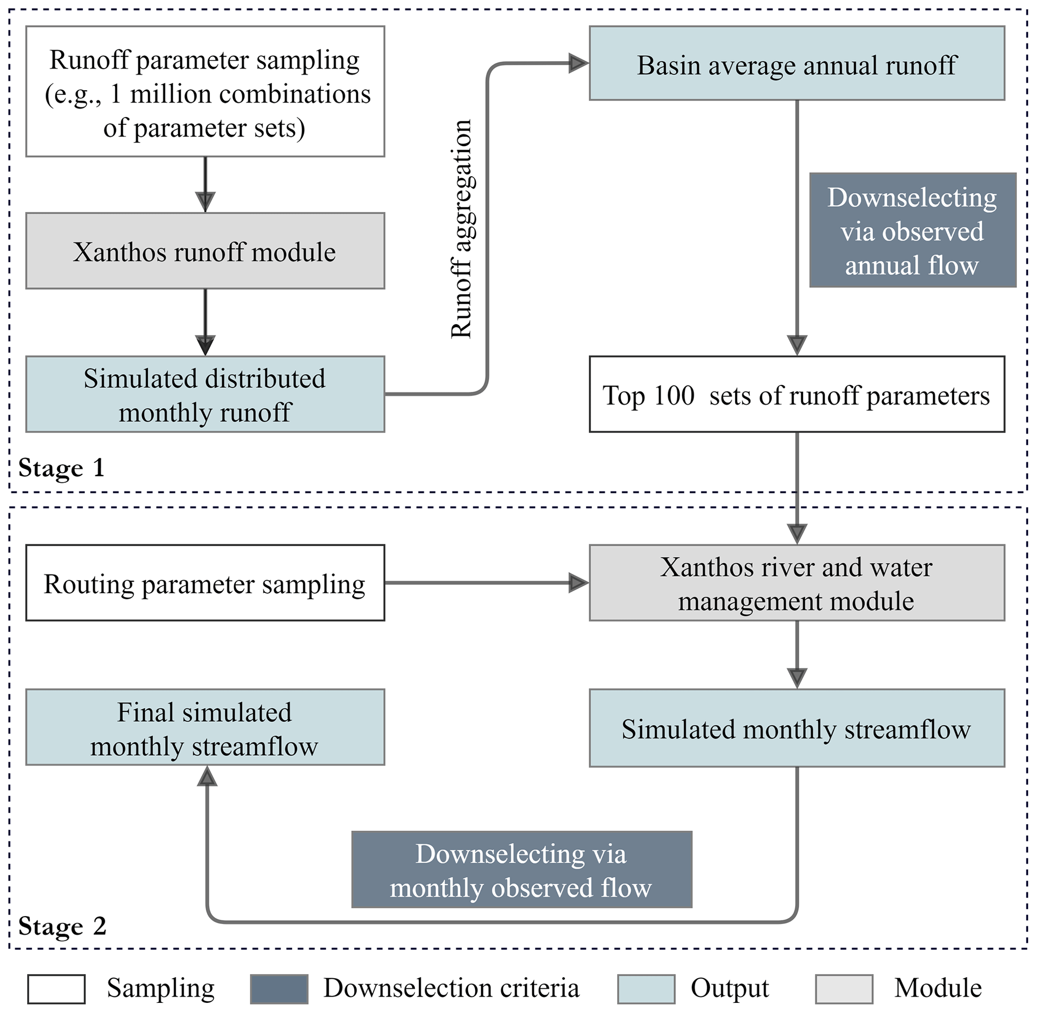
Figure 2Runoff and routing parameters selection strategy for Xanthos-enhanced. Each component of the process is categorized as one of the following: (1) sampling, wherein parameter combinations are sampled; (2) downselection criteria, which are applied to downsample a larger parameter set into a smaller, more favorable subset; (3) outputs, which describes model outputs; and (4) modules, which describes Xanthos model methods (or sections of code).
In the first stage, we determine the optimal values for the five parameters in the runoff-generation module (see Table 2) in four steps. (1) We generate 1 million runoff parameter combinations using a Latin hypercube sampling (LHS) scheme (McKay et al., 1979; Fig. S1 in the Supplement). LHS is a statistical method for multidimensional parameter space sampling. The stratified sampling strategy employed by LHS ensures that all portions of the sampling space are represented (McKay et al., 1979). The user decides on the required number of parameter combinations and the upper and lower bounds of the individual parameters. Based on that, LHS simultaneously stratifies all input dimensions. (2) For each runoff parameter combination, we execute the runoff module to produce the simulated monthly total runoff time series at each grid cell in the study period. In this study, we uniformly apply the same parameter values to all the grid cells in a basin to generate a monthly runoff time series at each grid cell. Parameter values vary among basins, just not across grid cells within a basin. (3) We calculate the simulated annual runoff depth at each grid cell. We then take the spatial average across the grid cells within the upstream drainage area of a gauge station where observed streamflow data are available; this is denoted as Qsim_annual (mm yr−1). (4) At the river gauge station, we calculate the long-term mean of observed streamflow and divide it by the drainage area, Qobs_annual (mm yr−1). We then select the top 100 runoff parameter combinations that produce the smallest normalized root mean square error (NRMSE) between Qsim_annual (the annual water consumption) and Qobs_annual.
Before these 100 runoff parameter combinations are passed onto the second stage, the runoff generated by the top 100 parameters is further evaluated at the mean monthly scale to confirm that the selected parameter combinations yield reasonable runoff simulations in terms of timing. For this purpose, we compare the peak time of the simulated mean monthly runoff (i.e., the calendar month in which the mean monthly runoff is highest; hereafter denoted as simulated peak runoff time) with that of Global Runoff Data Center (GRDC) mean monthly flow (i.e., the calendar month when the mean monthly flow is highest; hereafter denoted as observed peak flow time; Fig. S2). Note that the mean monthly runoff employed here is a simple spatial average with no channel routing. Therefore, a reasonable simulated peak runoff time is expected to be earlier than the observed peak flow time by 0–3 months. The range of 0–3 months is estimated by applying a 1.0 m s−1 travel velocity to the longest river in the world, the Nile River, which yields a total travel time between 2.0 and 3.0 months.
The selected 100 parameter combinations are then passed on to the second stage, where we determine the final optimal parameter set in four steps. (1) We set the reservoir capacity reduction factor (α) to a value of 0.85, following Hanasaki et al. (2006). (2) The channel velocity adjustment coefficient (β) is sampled in a relatively uniform manner within the range of 0.1–10.0. In total, there are 19 possible β values to be considered (i.e., β=0.1, 0.2, 0.3, 0.4, 0.5, 0.6, 0.7, 0.8, 0.9, 1.0, 2.0, 3.0, 4.0, 5.0, 6.0, 7.0, 8.0, 9.0, and 10.0). (3) For each of the 100 selected runoff parameter combinations, we use the corresponding simulated runoff time series as the inputs and run the river and water management modules 19 times (each time corresponds to one of the 19 β values and α=0.85) at a 3 h time step. (4) We validate the simulated streamflow time series at the grid cell (where the gauge station is located) against the observed monthly streamflow time series. From step (3), there are 1900 simulations for each basin, each corresponding to a combination of five runoff parameters and one routing parameter (a, b, c, d, m, and β). The final optimal parameter set is the one that produces the best model performance (per the performance metrics discussed in the following Sect. 2.5). Note that within each basin, we held the set of parameters constant across the cells, which is a reasonable simplification since, typically, there is no sufficient observational data to effectively capture the spatial heterogeneity of these parameters within each basin.
This new strategy has several benefits. First, it largely alleviates the equifinality issue by effectively sampling the whole parameter space. Our experimental design covers the full theoretical value range for each of the six parameters. Second, it reduces the computational burden to a reasonable level. Our suggested approach includes 1 million model runs for the runoff module at the monthly time step for each river basin and another 1900 runs for the river-routing and water management modules at the 3 h time step. We suggest that this new strategy applies to those hydrologic modeling frameworks where (1) some module(s) is (are) computationally much cheaper than the others, and (2) these modules must run sequentially instead of simultaneously. A demonstration of this parameter determination strategy is provided in Sect. 3.
2.5 Metrics for model assessment
To evaluate model performance, we use the Kling–Gupta efficiency (KGE; Gupta et al., 2009), which is given by
where , and μobs are the standard deviation of streamflow value for a given simulation, the standard deviation of observed streamflow, the simulated mean, and the observed mean values, respectively. A higher KGE indicates a better degree of agreement between the simulated and observed variables, and a KGE value of 1.0 indicates perfect agreement. The KGE value is −0.41 if the simulated monthly flow equals the observed long-term mean flow for all months (Knoben et al., 2019).
While KGE is a useful means of evaluating the skill of a particular set of model parameters in reproducing observed streamflow, we also wish to directly compare simulation outputs against one another across multiple model configurations and parameterizations for both reservoir storage and reservoir release. To enable this comparison, we employ the following indices that capture key aspects of the regulation behavior of reservoirs.
-
Reservoir impact index (RII). RII is the ratio of a reservoir storage capacity (C) in meters cubed to annual mean flow (Qmean; López and Francés, 2013; Wang et al., 2017). RII is similar to the Hanasaki scheme's degree of regulation term, except that RII is computed at the GRDC site instead of the reservoir site. Low and high values of RII indicate that the stream is lightly and heavily regulated, respectively.
where Qmean is the observed annual mean flow at the GRDC site (in m3 yr−1).
-
Seasonality index (SI). SI represents the degree of variability in the monthly release or storage within a year and is computed with the Walsh and Lawler (1981) method.
where Xm is the mean monthly value for the month m, and is the annual mean value. SI ranges between 0 and 1.833, indicating uniform distribution over the 12 months and a single-month occurrence, respectively. When applying this equation, use units that represent a measure of water quantity over a month, such as depth (e.g., millimeters per month) or volume (e.g., meters cubed per month).
-
Coefficient of variation (CV). CV is the ratio of standard deviation to mean and is employed here to depict the extent of interannual variability in storage and release.
No reliable global observational datasets exist for reservoir storage levels and releases, so it is difficult to establish whether the metric values (for RII, SI, and CV) from one model configuration versus another are closer to reality. Despite this limitation, comparing metric values across simulations is still useful for understanding the effects of modeling assumptions (e.g., representing hydropower reservoirs as such instead of as flood control reservoirs). To enable comparison, we measure the difference or closeness between two alternative time series, representing two alternative model configurations or parameterizations, using normalized root mean square error (NRMSE) and coefficient of determination (R2). NRMSE typically captures the magnitude difference between two time series, while R2 measures the proportion of the variance explained (Moriasi et al., 2007).
2.6 Metrics for sensitivity analysis
As we have discussed, equifinality is a crucial issue when calibrating a hydrological model that is highly parameterized. To assess model robustness, it is important to evaluate how sensitive the model's performance is to each model parameter. The sensitivity analysis approach we propose here is moderately different from traditional methods, since we implement a novel parameter determination strategy (see Sect. 2.4). The sensitivity analysis aims to identify the most and least influential model parameters. Such an understanding can help identify priorities of parameter estimation in future works and simplify or improve the model structure. Two separate sensitivity analyses are performed. The first sensitivity analysis is performed before the parameter selection, using results from all 1 million parameter sets. Here, an NRMSE for each of the 1 million parameter sets was computed between simulated annual runoff and observed annual runoff. The annual runoff is observed as annual streamflow converted to an equivalent depth over the upstream contributing basin area. The simulated annual runoff is calculated by subtracting the basin's annual water consumption from the total runoff. The correlation coefficient was then computed between an array of the computed NRMSE and each runoff parameter to evaluate the correlation between the change in parameter values and model performance. We computed five correlation coefficients from the 1 million runs (i.e., between model performance and the five runoff parameters for each basin).
After applying the new parameter selection strategy, the second sensitivity analysis is carried out on 1900 samples (i.e., samples generated from combining the 100 samples from the first stage with 19 discretized β values). Each sample includes the five runoff parameters and the velocity adjustment coefficient employed for streamflow simulation during the second stage. Here, the model performance (KGE) is computed between the monthly observed and simulated streamflow. We switched to KGE for the monthly time series evaluation, as we are interested in metrics that reflect the agreement in both magnitude and patterns of monthly flow. The correlation coefficient is computed between the KGE and each parameter. We obtain six correlation coefficient values for each basin, corresponding to the five abcd model parameters and the routing parameter (i.e., β). As with its interpretation in stage 1 of the sensitivity analysis, here a higher correlation coefficient between a parameter's values and the corresponding performance metric (in this case, KGE) suggests that the variance in model simulation outcomes is more strongly related to the changes in the target parameter and hence more sensitive to this parameter.
We apply Xanthos-enhanced over the global domain at a 0.5∘ resolution and monthly time step. The study period is 1971–1990, based on the availability of forcing and observed streamflow data over all the basins. We divide the study period into a calibration period, 1971–1980, and a validation period, 1981–1990.
3.1 Data and numerical experiments
For this study, we obtain gridded global monthly climatic data, including precipitation, maximum temperature, and minimum temperature, from the WATer and global CHange (WATCH; Weedon et al., 2011) dataset, which covers the period 1971–2001. We obtain global reservoir data from the GRanD dataset (Lehner et al., 2011; Fig. 3a). Monthly water demand and consumptive water use data for various sectors at a 0.5∘ resolution are from Huang et al. (2018b, a), which are available from 1971 to 2010 (Fig. 3c). Observed streamflow data for model parameter identification and validation are obtained from the GRDC (https://www.bafg.de/GRDC, last access: 1 August 2022). We begin by comparing Xanthos' corresponding MRTM upstream area (after locating each gauge station within a Xanthos grid cell) with the GRDC gauge contributing area. If the drainage area difference is larger than ±20 %, then we look for an option to readjust the station to one of the eight neighboring grid cells. Here, only gauges within ±20 % in area difference (3097 GRDC gauges) are retained for further use in this study. Temporal filtering of these gauges with the availability of 20 years (1971–1990) of continuous data reduced the number of stations to 1178. These gauge stations are located within 91 of the 235 Xanthos basins. For model validation purposes, we select the GRDC gauge with the largest upstream area within each basin, i.e., 91 GRDC gauges in total (Fig. 3b).
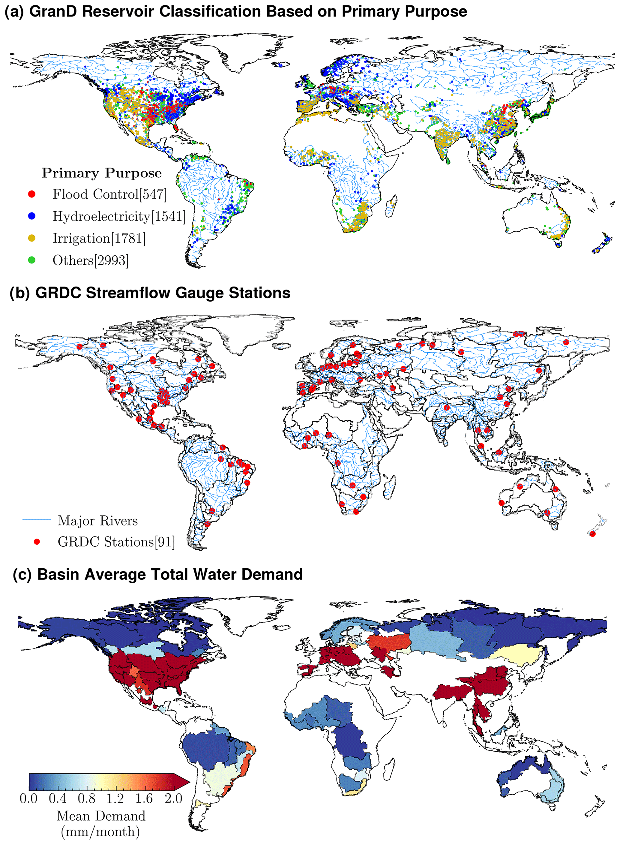
Figure 3Global data used in this study. (a) Global distribution of 6862 reservoirs from the GRanD database classified, based on the primary reservoir purpose. (b) GRDC stream gauge stations in 91 basins where data were of sufficient length, quality, and upstream watershed contributing area for use in this study. (c) Basin mean monthly water demand in those same 91 river basins.
The GRanD database we use here only considers reservoirs with storage capacity values greater than 0.1 km3. We also exclude reservoirs with missing storage capacity values and those identified with purposes such as tide control, which reduces the total GRanD reservoirs from 6862 to 6847. For any grid cell with more than one reservoir, we aggregate all of the reservoirs located locally (i.e., within the grid cell) into a single reservoir with a storage capacity equivalent to that of the local reservoirs combined. The purpose of the combined storage is determined by the two steps described in Sect. 2.3. As a result of this process, the 6847 GRanD reservoirs are remapped into 3790 reservoirs. Among the 3790 reservoirs, 1095, 598, and 2097 are categorized as irrigation, hydropower, and flood control and others, respectively (Fig. 1). Furthermore, out of the 3790 global reservoirs, only 1878 of them are located within the 91 basins simulated in this study. Out of these 1878 reservoirs, the primary purpose is hydropower for 296, irrigation for 486, and flood control or others for 1096. The reservoirs across these 91 basins make up approximately 66 % of the total dams within the GRanD dataset. The construction years of these dams pose a critical factor in deciding the starting year of the calibration. Here, we found that ∼ 69.5 % of these dams were constructed before 1971, and an additional ∼ 17.2 % were built between 1971 and 1981. We considered it reasonable to include all dams, regardless of their construction year, in the calibration starting from 1971, mainly for the following two reasons: (i) incrementally aggregating dams built during this period over time, in addition to the dams built before 1971, would significantly complicate the modeling process; and (ii) dams constructed before 1981 account for approximately 84 % of the total storage within these basins.
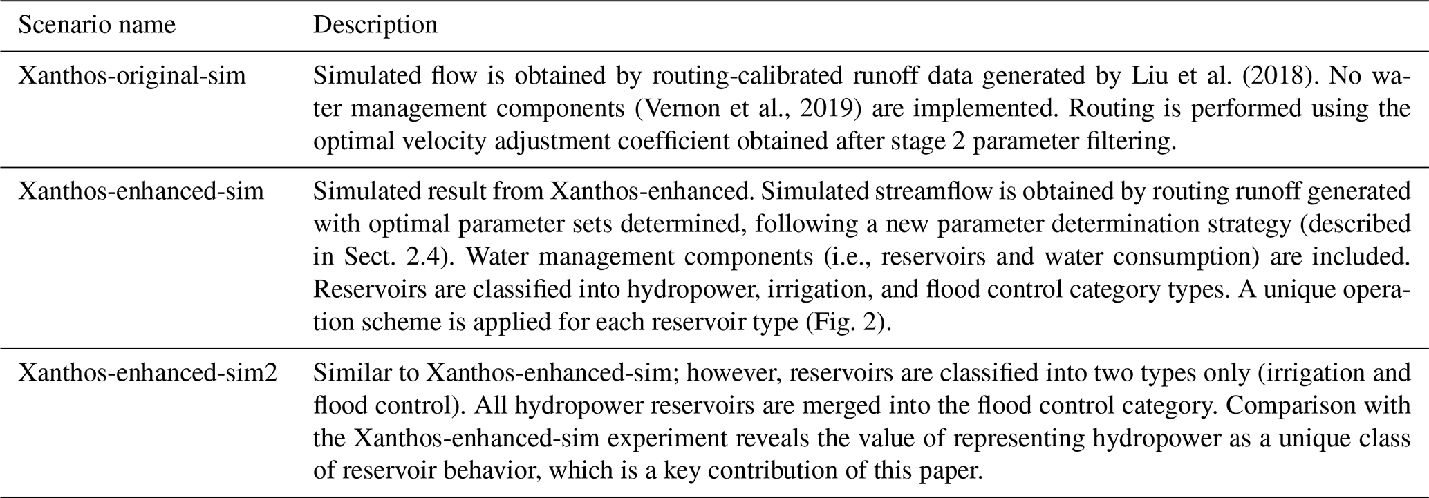
With the aforementioned data, we carry out three global simulations to explore the performance of the Xanthos-enhanced (see Table 3). These include (1) a simulation with Xanthos-original, denoted Xanthos-original-sim, where the simulated flow is obtained by routing-calibrated runoff data generated by Liu et al. (2018) with calibrated abcd model parameters but no water management; (2) a simulation with Xanthos-enhanced, denoted Xanthos-enhanced-sim, where we run the runoff, river-routing, and water management modules with the final optimal parameter values determined, following the new strategy as outlined in Sect. 2.4; (3) a simulation similar to Xanthos-enhanced-sim but one that treats all the hydropower reservoirs as flood control reservoirs (denoted Xanthos-enhanced-sim2). By comparing Xanthos-enhanced-sim with Xanthos-original-sim, we demonstrate the overall improvement of model performance from Xanthos-original to Xanthos-enhanced, due to a combination of the new parameter determination strategy and new water management module. Note that in Liu et al. (2018), the traditional, brute-force calibration strategy was invoked, since Xanthos-original only consists of a monthly runoff-generation module and runs very quickly. By comparing Xanthos-enhanced-sim with Xanthos-enhanced-sim2, we isolate the net difference between simulating hydropower reservoirs based on Eq. (3) and the traditional approach employed by GHMs (i.e., treating hydropower reservoirs as flood control reservoirs, based on Eq. 4).
3.2 Parameter determination outcomes
We apply the two-stage model parameter determination strategy described in Sect. 2.4, using the global datasets described in Sect. 3.1. The LHS generates a parameter set using defined bounds (see Fig. S1 in the Supplement). Here, we describe the results from the implementation of the two-stage strategy, using the Amazon basin as an example. A subset of 100 good parameter sets (filtered) are identified among the 1 million parameter sets (raw; see Fig. S2a in the Supplement). The mean monthly runoff generated with the subset and the observed mean monthly runoff (see Fig. S2b in the Supplement) showed that the simulated runoff peak time is earlier than the streamflow peak time and within the 1–3-month range established in Sect. 2.4. The model's integrity is contingent upon the theoretical expectation of the streamflow peak trailing the runoff peak by a span of days to months. Any set of parameters resulting in a reversed pattern, where the runoff peak occurs later, is deemed unacceptable due to possible anomalies within the model.
The peak time differences (i.e., the difference between GRDC mean monthly peak flow time minus simulated runoff peak flow time) corresponding to the selected sets of parameters are among the best of the 1 million samples when ranked in an ascending order, based on an absolute value of the peak time difference (see Fig. S2c in the Supplement). The robustness of the implemented procedure is justified by the presence of a range of parameter values between their upper and lower bounds (see Fig. S2d in the Supplement), indicating that the selected parameters are not concentrated within a specific parameter space. These characteristics have also been observed in most of the basins evaluated for this study (figure not shown). We select one parameter combination for each basin that results in the best KGE value. The spatial maps of the final optimal parameter values are shown in Fig. S3 in the Supplement. In most cases, optimal values for parameter a are close to the upper bound, while those of parameter d are closer to the lower bound. Parameter b is low in basins in the high-latitude sub-region; to some degree, this may be attributed to the fact that, in general, evapotranspiration decreases towards most of the high-latitude regions. Parameter c seems to be lower in the eastern hemisphere and has relatively no distinct pattern in the western hemisphere basins. The snowmelt parameter m is only above zero in regions with significant snow contributions. The parameter β is higher in high-latitude basins. β was only introduced to readjust the global velocity data after noticing bias in the monthly flow timing at many sites; hence, applications of our methodology that use more reliable velocity data should consider setting β to a value of 1. The high values of β in the higher-latitude basins could be attributed to the original velocity estimation approach's systematic bias in cold regions (Li et al., 2015).
3.3 Global evaluation
Overall, Xanthos' performance has improved after adding the water management module. Figure 4 shows violin plots of KGE between the GRDC monthly observed streamflow and those simulated from the Xanthos-original-sim and Xanthos-enhanced-sim simulations for the 91 basins during the calibration (Fig. 4a) and validation (Fig. 4b) periods, respectively. In most cases, during both calibration and validation periods, the Xanthos-enhanced-sim simulation's KGE values are consistently higher than those of the Xanthos-original-sim simulation. For the Xanthos-enhanced-sim simulation, the KGE value is no less than 0.5 and 0.0 for 59 and 89 basins during the calibration period and 39 and 81 basins during the validation period, respectively.
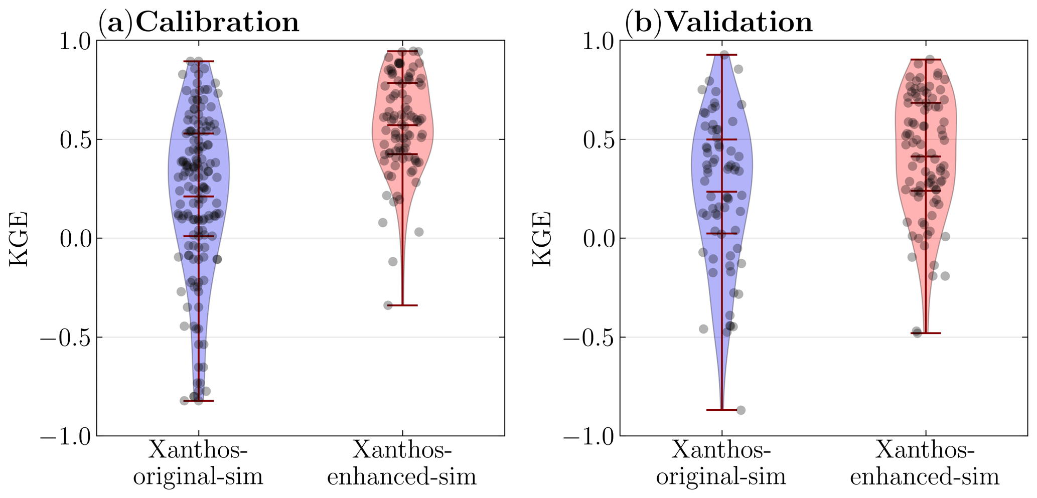
Figure 4Box plots of the KGE values for the Xanthos-original-sim and Xanthos-enhanced-sim simulations during (a) the calibration period (1971–1980) and (b) the validation period (1981–1990). In this plot, the outliers (KGE values lower than −1) are not shown. For Xanthos-original-sim, 77 basins in calibration and 70 basins in validation are shown. For Xanthos-enhanced-sim, 91 basins during calibration and 89 during validation are shown.
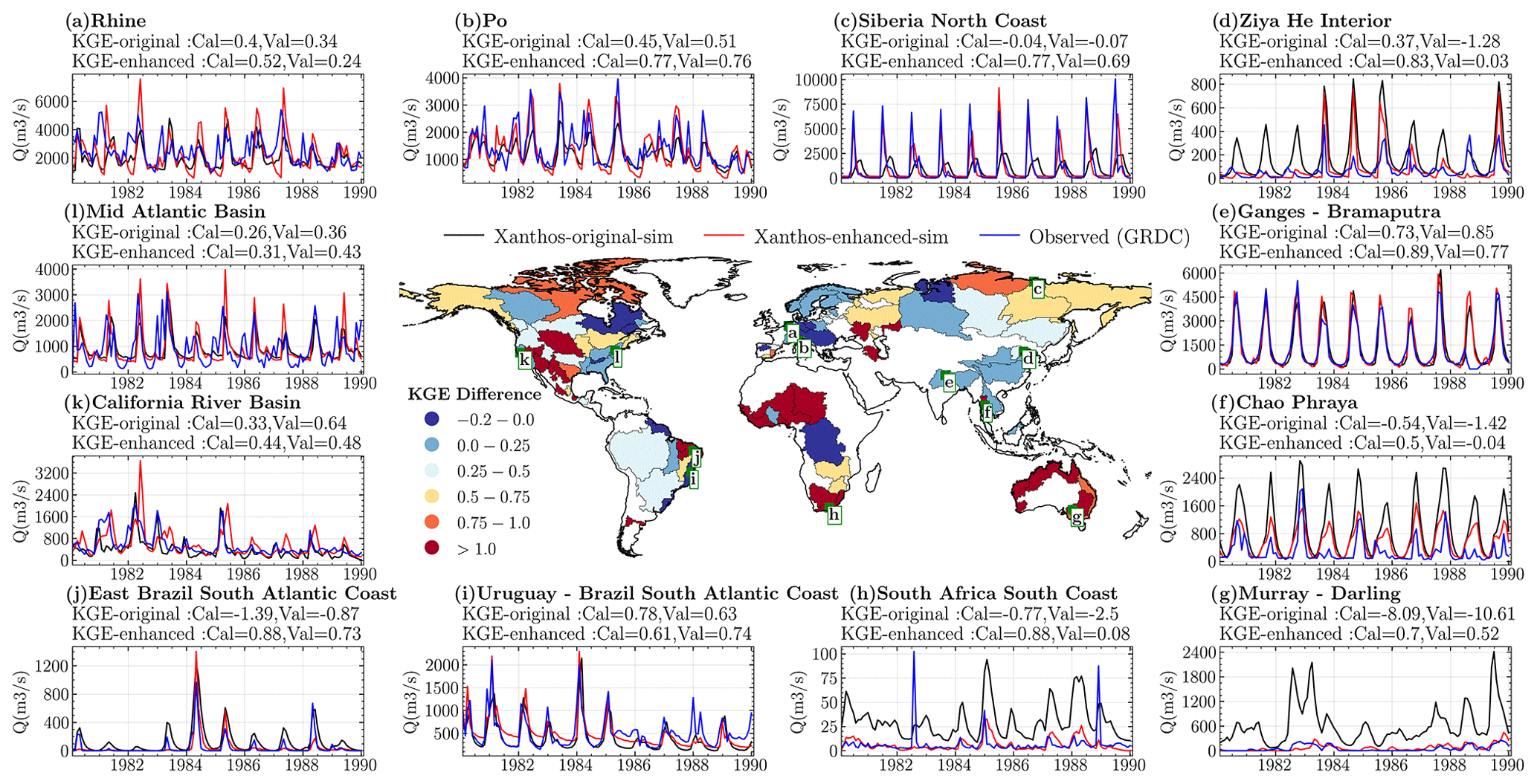
Figure 5Spatial maps of basin-specific difference between the KGE values from Xanthos-enhanced-sim and those from Xanthos-original-sim for the calibration period 1971–1980 (map at center), where a value greater than zero indicates improved performance from the addition of water management features to Xanthos. The time series plots are simulated and observed monthly streamflow for basins with the highest water demand in different global regions during the validation period (1981–1990). KGEcal is the KGE during the calibration period, while KGEval is the KGE during the validation period.
Figure 5 provides a comprehensive comparison of the Xanthos-enhanced-sim and Xanthos-original-sim, emphasizing the impact of water management integration. This is illustrated both spatially, through a map depicting KGE differences, and temporally, via time series plots for selected basins. Overall, by incorporating this element, improvements are noticeable in the KGE values of 75 basins, thus indicating a better simulation accuracy for these basins. The increase in KGE values is substantial and exceeds 0.05 when compared to those of the Xanthos-original-sim. However, it is also crucial to note that the water management integration negatively affected the KGE values (i.e., KGE values decreased by more than 0.05) in seven basins. In the remaining nine basins, KGE did not significantly change. For basins in which performance worsened, the decrease in performance is likely due to factors such as the uncertainties in the climate forcing data and GRDC streamflow observations (Moges et al., 2021) and the lack of spatial heterogeneity in the estimated parameters at the sub-basin scale (i.e., the parameters are uniform across all grid cells in a given basin). The distribution and operational patterns of reservoirs, particularly in relation to their closeness to gauge stations, could also represent a nontrivial contributing factor to this issue.
To further examine Xanthos' performance in more detail, Fig. 5 also shows the monthly time series of simulated and observed streamflow at the 12 GRDC stations (out of the 91 evaluated here) with relatively higher average annual water demand in their geographical region (see Fig. 3c) and hence stronger water management effects. The 12 basins are the Rhine, Po, Siberia north coast, Ziya He interior, Ganges–Brahmaputra, Chao Phraya, Murray–Darling, South Africa south coast, Uruguay–Brazil South Atlantic coast, east Brazil South Atlantic coast, California basin, and mid Atlantic. Compared to Xanthos-original, Xanthos-enhanced-sim better captures the seasonal variations in the streamflow, more closely matching the observed streamflow during the high-flow and low-flow periods. This highlights the importance of the reservoir regulation effect (e.g., attenuating high flows and augmenting low flows) that Xanthos-original has not captured.
3.4 Parameter sensitivity analysis
To identify which parameters are most critical (i.e., contribute most to the variance in key model outputs), we evaluate the sensitivity of the model's performance to the changes in a, b, c, d, m, and β, as shown in Fig. 6. Note that we fix the value of α at 0.85, following Hanasaki et al. (2006), in this study. We first carry out the sensitivity analysis on the runoff parameters based only on the first-stage parameter determination results (Fig. 6a). The results show a significant sensitivity (correlation coefficient > ) only for parameters a (which represents the propensity of runoff to occur before the soil is fully saturated) and b (which represents an upper limit on the sum of evapotranspiration and soil moisture storage). The correlation between parameter a and the model performance is negative, indicating that it is inversely related to the NRMSE computed from annual observed and simulated runoff. Parameter a controls the volume of runoff generation when soil is undersaturated, and the relationship suggests that annual runoff is estimated better when saturation excess runoff is not the primary process. Parameter b controls the soil saturation level. Hence, it is responsible for the memory of the basin. Therefore, the positive correlation indicates that the difference between simulated and observed annual runoff increases as the basin memory increases.
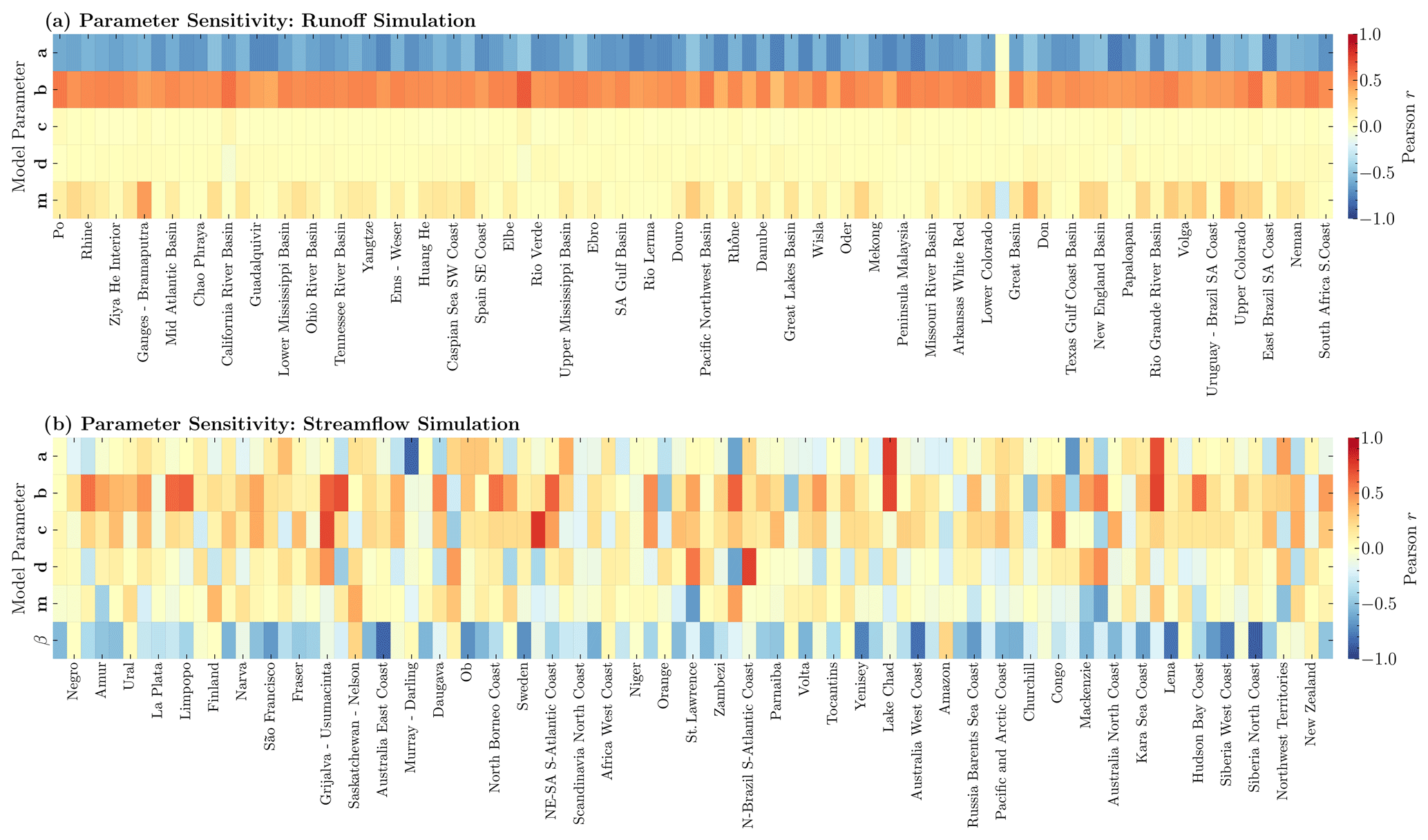
Figure 6Parameter sensitivity analysis for Xanthos-enhanced in the form of the Pearson correlation coefficient (Pearson r) (a) between runoff parameters (i.e., 1 million parameter sets) and their corresponding normalized root mean squared error (NRMSE) computed with annual runoff; and (b) between streamflow simulation parameters (i.e., the combination of the top 100 runoff parameter sets and sampled routing parameter) and KGE computed from streamflow simulated at monthly scale. A higher Pearson r implies that the model performance is more sensitive to the parameter. For instance, (a) Pearson r less than zero indicates a decrease in annual runoff NRMSE as the parameter value increases, while Pearson r greater than zero indicates a positive association between annual runoff NRMSE and parameter value. Note that out of the 91 basins, only half of the basin labels (i.e., the x-axis labels) appear on the first panel, and the other half appears on the second panel, but all labels apply to both panels.
A similar analysis is made for the set of parameters generated by combining the 100 best abcd model parameter sets with the velocity adjustment parameter (β; Fig. 6b). Here, it appears that β has a stronger influence on model performance than the other parameters. This is expected because the differences among the 100 selected runoff parameter combinations are supposed to be small (e.g., see Fig. S2a (filtered) in the Supplement for the Amazon basin). For β, the sensitivity corresponds to an adjustment in the flow timing, leading to improved KGE. Note that this parameter can be avoided with a better estimate of spatially and temporally varying flow velocity. Considering these observations, it becomes evident that an enhanced parameterization of this variable, along with the other variable used to estimate the grid's water residence time (i.e., channel length), warrants increased attention. Hence, in the future, proper generation and integration of these components are crucial for boosting the model's accuracy and robustness, given their pivotal role in the MRTM-flow-routing process.
3.5 Hydropower reservoirs
Among the 91 basins we studied here, 51 have one or more hydropower reservoirs included in GRanD and hence in our simulations. Recall that these reservoir counts reflect our lumping of multiple reservoirs together within any given grid cell, so 296 reservoirs in our methodology reflect 433 actual reservoirs. At each of the 296 reservoirs, the simulated release and storage time series from Xanthos-enhanced-sim2 are compared with those from Xanthos-enhanced-sim to identify the benefit of capturing hydropower operations.
Figure 7 compares Xanthos-enhanced-sim and Xanthos-enhanced-sim2 with regard to intra-annual (Fig. 7a and b) and interannual (Fig. 7c and d) variability. The seasonality index (SI) summarizes the intra-annual variability; weak seasonality (i.e., low SI) indicates that most months contribute significantly to the annual magnitude, and strong seasonality (i.e., high SI) indicates that very few months contribute to the annual flux magnitude. Although SI showed more difference, both the SI and coefficient of variation (CV; which summarizes interannual variability) for release fall on the 1:1 line for most reservoirs (Fig. 7a and c), indicating that in most cases, the two scenarios have less impact on the intra- and interannual variability in the release. On the other hand, both SI and CV values for storage at most reservoirs show a significant difference, indicating that the two experiments significantly disagree in terms of the interannual and intra-annual variability in the storage. We emphasize that the significant takeaway from this comparison is not that one experiment's storage and release simulations are more variable than the other but that the two experiments led to substantially different seasonal and annual patterns. This highlights the drawbacks of representing hydropower reservoirs as flood control reservoirs.
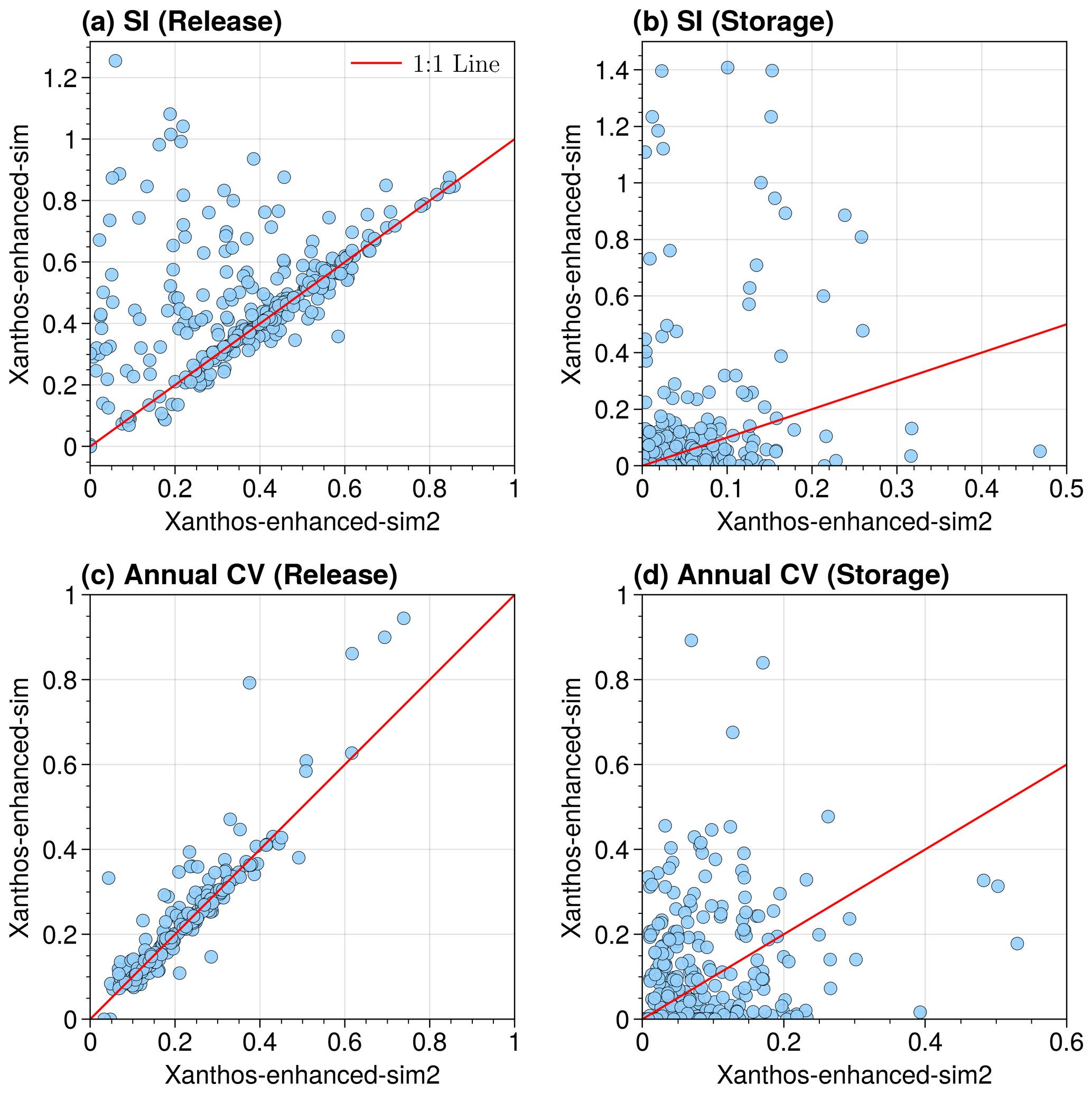
Figure 7Comparing intra-annual and interannual variability in the storages and releases simulated with the hydropower reservoirs of Xanthos-enhanced-sim and Xanthos-enhanced-sim2 experiments distributed over the 91 basins. (a) Seasonality index (SI) for release, (b) seasonality index for storage, (c) coefficient of variation (CV) for release at the annual scale, and (d) coefficient of variation (CV) for storage at the annual scale. The red line is a 1:1 line, where both scenarios are equal.
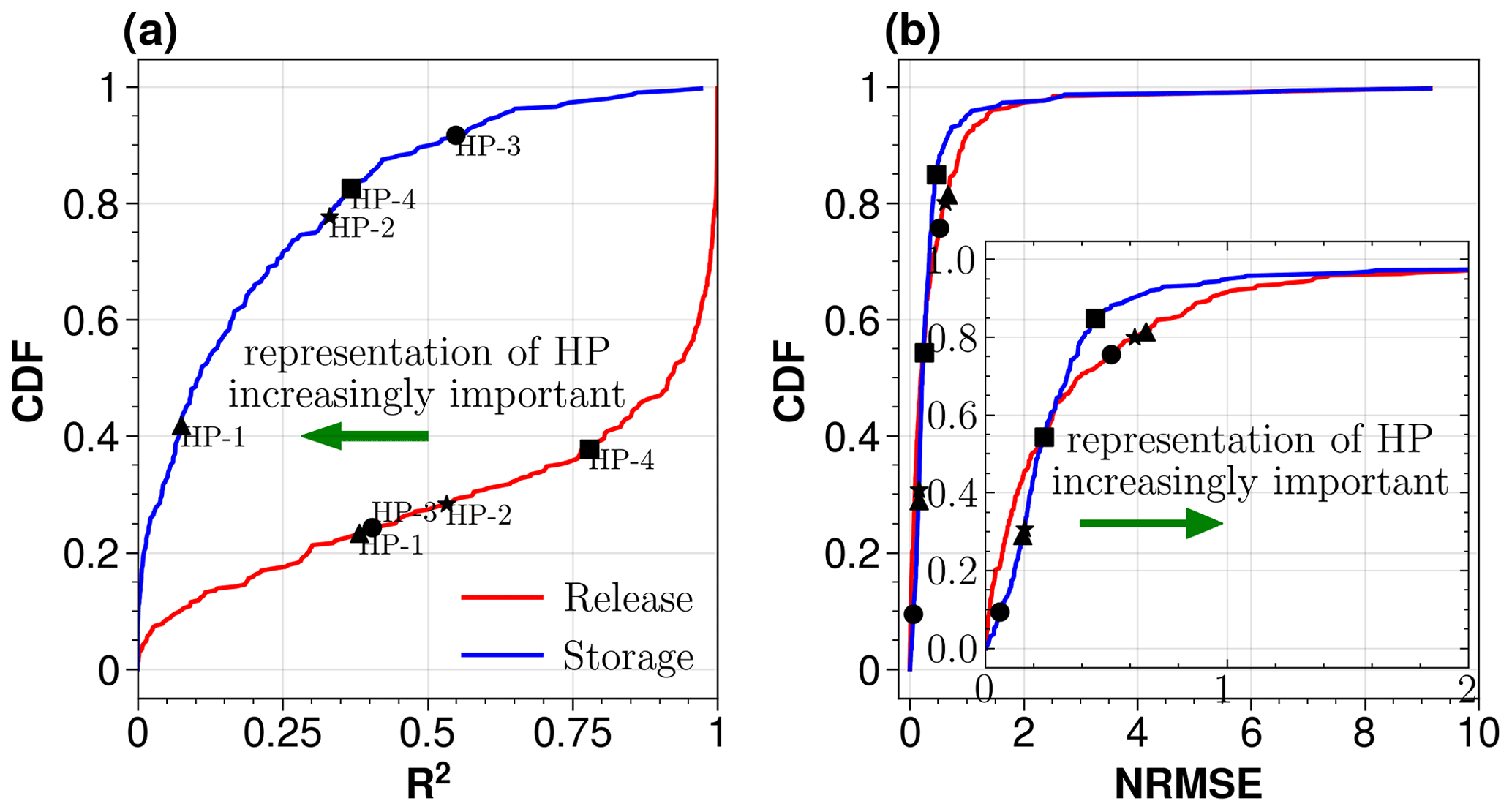
Figure 8Empirical cumulative distribution function (CDF) of reservoir storage and release R2 (a) and NRMSE (b) between Xanthos-enhanced-sim and Xanthos-enhanced-sim2 monthly simulations across all hydropower reservoir sites. The R2 CDF plot demonstrates that we produce very different storage and release patterns by accounting explicitly for hydropower reservoir functionality in Xanthos-enhanced-sim, although the difference in magnitude, as indicated by NRMSE CDF, is small. A higher R2 of 1.0 and NRMSE of 0.0 represent a perfect agreement between the two simulations, indicating that distinguishing between the representation of hydropower and flood control behavior was less important for basins with those values. The CDF plot is made of 296 hydropower reservoirs distributed across 51 basins. The labels on the plots (HP-1, HP-2, HP-3, and HP-4) correspond to hydropower reservoirs located upstream of the Yenisey basin's GRDC site (see Fig. S5 in the Supplement), as discussed in Sect. 3.5. The markers for these labels are similar for both panels (a) and (b).
Figure 8 summarizes the reservoir storage and release comparisons between Xanthos-enhanced-sim and Xanthos-enhanced-sim2 with an empirical cumulative distribution function (CDF) that plots R2 (and/or NRMSE) values across all 296 hydropower reservoirs, according to their rank-ordered exceedance probabilities. The spatial map for the comparisons is also shown in Fig. S4. Recall that a high NRMSE value means a significant magnitude difference between the two different time series, and a low R2 value means a significant timing difference. Of the 296 reservoirs, the simulated reservoir releases differ significantly between the two model configurations in ∼ 45 % of reservoirs in terms of magnitude (if we set a threshold at NRMSE > 0.25; Fig. 8b) and at only ∼ 28 % in terms of timing (if we set a threshold at R2<0.5; Fig. 8a). According to Fig. 8a and b, treating hydropower reservoirs as flood control reservoirs does not significantly impact the model simulated reservoir releases from most reservoirs, which partly supports the lack of differentiation between hydropower and flood control reservoirs in previous studies. However, the simulated reservoir storages are significantly different for ∼ 44 % of the 296 reservoirs in terms of magnitude (NRMSE > 0.25; Fig. 8b) and ∼ 90 % in terms of timing (R2<0.5; Fig. 8a). Treating hydropower as flood control reservoirs thus has much more impact on the simulation of reservoir storage than release, particularly in terms of timing. The NRMSE and R2 values in Fig. 8 do not appear to relate to the reservoir sizes (figure not shown).
To explore the dynamics responsible for these broad patterns in Fig. 8, we select the Yenisey basin here to study them in more detail. Here, the Yenisey basin is selected for demonstration because it has a mix of only flood control and hydropower reservoirs and has just six reservoirs upstream of the GRDC site. In the Yenisey basin, the upstream area of the GRDC station is dominated by hydropower reservoirs, i.e., four hydropower reservoirs and two flood control, as shown in Fig. S5a in the Supplement. Note that one of the two flood control reservoirs is located downstream of the hydropower reservoirs (Fig. S5a). This spatial arrangement allows us to evaluate the effects of simulating hydropower reservoirs as flood control reservoirs without interference from the third purpose (i.e., in cases where an irrigation reservoir is located downstream of a hydropower reservoir). Figure S5b (see the Supplement) shows the total simulated storage (sum of all six reservoirs) from Xanthos-enhanced-sim2 and Xanthos-enhanced-sim. The difference in the magnitude of total simulated storage between the two simulations is very significant (KGE between them is 0.44). In Xanthos-enhanced-sim2, where all reservoirs are simulated as flood control, the storage is relatively more variable from month to month, while Xanthos-enhanced-sim changes are more smooth, likely because the release aims to maintain mean annual flow in Xanthos-enhanced-sim2, which leads to releases that exceed inflow during the drier seasons and quick fill-up during the wet seasons. The streamflow comparison at the GRDC site (Fig. S5c in the Supplement) indicates that the difference in the simulated reservoir releases is also significant. The KGE values drop from 0.366 to 0.152 during the calibration period (1971–1980) and from 0.293 to 0.008 during the validation period (1981–1990) when simulating the hydropower reservoirs as flood control.
For those basins where hydropower reservoirs serve a secondary purpose compared to irrigation, flood control, or other types of reservoirs, there is no significant difference in the KGE values between Xanthos-enhanced-sim2 and Xanthos-enhanced-sim, suggesting that treating hydropower reservoirs as flood control reservoirs will not lead to a significant difference in streamflow simulations at the regional or basin level. Figure 9 depicts the RII of the hydropower reservoirs on flow at GRDC stations for basins with one or more hydropower reservoirs (i.e., 51 of the 91 basins). The RII, shown here, corresponds to a hydropower reservoir with the largest storage within the basin. Figure 9 also shows a time series plot of the relative difference between Xanthos-enhanced-sim2 and Xanthos-enhanced-sim storage and release for 10 basins with relatively higher RII within different geographic regions.
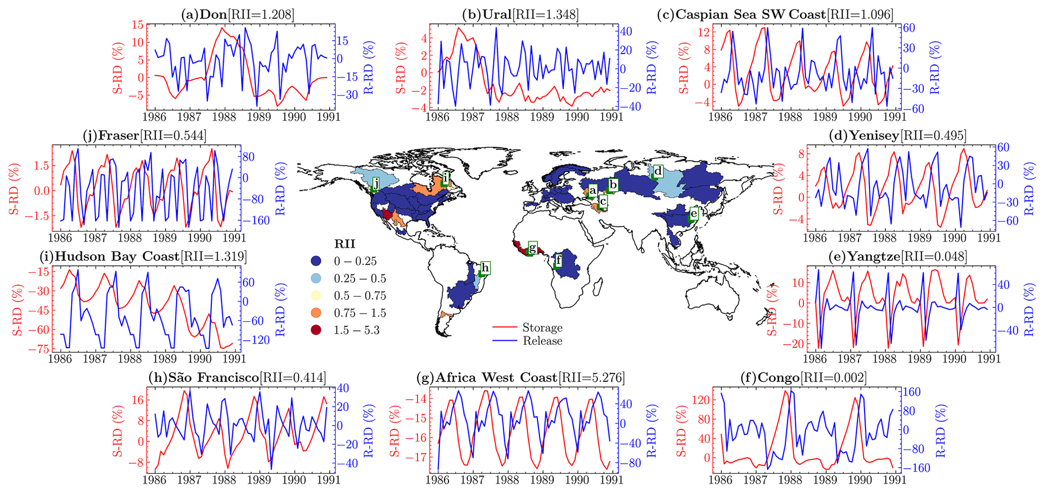
Figure 9The difference between reservoir storage and release monthly time series between Xanthos-enhanced-sim and Xanthos-enhanced-sim2 simulations at hydropower reservoirs demonstrates the value added by explicitly accounting for hydropower reservoir functionality in Xanthos-enhanced-sim. The reservoir impact index (RII) is the ratio of reservoir storage capacity (in cubic meters) to annual mean flow (in cubic meters). Low and high values of RII indicate that the stream is lightly and highly regulated, respectively. For instance, RII > 1.0 shows the reservoir's capacity to shift the downstream flow below the annual mean flow. The map at the center of the figure displays the RII for the hydropower reservoir with the largest RII in each basin. In other words, each basin is represented by one hydropower reservoir with the largest impact on flow at the GRDC site. The times series plots show the storage relative difference (S-RD) and release relative difference (R-RD) between the two scenarios. For example, S-RD represents Xanthos-enhanced-sim storage minus Xanthos-enhanced-sim2 storage scaled by the mean of the two storages.
The time series plots in Fig. 9 show the storage relative difference (S-RD) and release relative difference (R-RD) between the two scenarios. S-RD represents Xanthos-enhanced-sim storage minus Xanthos-enhanced-sim2 storage scaled by the mean of the two storages. Similarly, R-RD is the scaled difference in the simulated releases. From the time series plots of S-RD, one can see that, in some example basins, S-RD is > 0 (Fig. 9). This characteristic implies that when a reservoir is simulated as a hydropower reservoir, it generally maintains high storage with less variation than when simulated as a flood control reservoir. This can be attributed to our release policy for hydropower simulation, which targets maximum long-term revenue, where reservoir storage level is an essential component. Out of the 296 reservoirs, about 150 of them demonstrate this type of behavior for at least 50 % of the study period (1981–1990).
Flow downstream of hydropower reservoirs is also influenced by the change in the reservoir purpose from hydropower to flood control (Fig. S5c in the Supplement). Similarly, a comparison of simulated releases (Fig. S6 in the Supplement) shows the difference between the simulated monthly releases in the peak and low-flow periods. On the one hand, the release from the flood control reservoirs is high during peak flow periods because they aim to create excess storage capacity to attenuate inflow during the next flood event. On the other hand, the release from the hydropower reservoirs can only go up to the maximum turbine flow plus spillover. The Hanasaki et al. (2006) approach readjusts the mean annual flow, depending on the reservoir's degree of regulation (i.e., capacity ratio to mean annual inflow). Therefore, in Xanthos, given that the readjusted mean annual flow is greater than the environmental flow (10 % of the mean annual flow), release remains constant during the low-flow periods. For hydropower reservoirs, low-flow releases are determined by a release policy intended to maximize revenue. Because of the changes in reservoir purpose, downstream reservoir releases are also modified.
Taken together, Figs. 7–9 and Figs. S4–S6 (in the Supplement) suggest that individual hydropower and flood control reservoirs behave very differently under the same climate and upstream conditions, particularly in terms of the simulated reservoir storage variations. Regarding regional-scale simulations, treating hydropower reservoirs as flood control leads to noticeably different simulated streamflow only in the basins, where hydropower reservoirs dominate over the other types of reservoirs. For instance, for the lower Colorado (RII = 1.92), Caspian Sea southwest coast (RII = 1.2), Yenisey (RII = 1.02), Hudson Bay coast (RII = 1.32), and São Francisco (RII = 0.67) basins, KGE improvement was > 0.1 over the calibration period. The indicated RII corresponds to the total effect of hydropower reservoirs located upstream of the basin's GRDC site. This observation will have critical implications in studies for which freshwater storage is the core interest, since reservoir storage is a critical component of terrestrial freshwater storage. For instance, the number of hydropower reservoirs in many global basins is rapidly increasing (Zarfl et al., 2015). Hence, the potential of simulating them in GHMs is vital, as the water use characteristics in many of these basins with hydropower reservoirs could change in the next decade or two if hundreds of new dams are built. Furthermore, the observed distinct characteristics between hydropower and flood control reservoir storages have substantial implications for reservoir sedimentation, which is another essential feature that the GHMs are increasingly looking to capture.
The results in this paper highlight some promising potential outcomes from accounting explicitly for hydropower objectives and operational behavior in GHMs. However, we note that it is premature to conclude from the above analysis that treating hydropower reservoirs as flood control leads to poor hydrological simulations, and vice versa. Many reservoirs, particularly large ones, serve multiple purposes, so their behavior is controlled by multiple factors. This study takes the same simplification strategy adopted by all existing GHMs, i.e., treating each reservoir as having a single purpose. Overcoming this simplification in a GHM setting is beyond the scope of this study and is left for the future.
This study adds a new water management module into the Xanthos model to improve its representation of global hydrological systems. The new water management module enhances Xanthos mainly by introducing reservoir regulation and local surface water withdrawal. We represent unique reservoir operation behavior for each reservoir based on its primary purpose, which can fall into the following three categories: irrigation, hydropower, and flood control and others. In particular, hydropower reservoirs have been treated as flood control reservoirs in previous GHM studies, while here we determined the operation rules for hydropower reservoirs via optimization that maximizes long-term hydropower production. We apply the enhanced Xanthos (Xanthos-enhanced) globally at a 0.5∘ spatial resolution and monthly time step. Validation against observed streamflow in 91 river gauge stations demonstrates improved performance over the original Xanthos (Xanthos-original) version. At the individual reservoir level, we show that hydropower and flood control reservoirs indeed behave quite differently, particularly in terms of reservoir storage variations. At the regional level, we show that treating hydropower reservoirs as flood control reservoirs leads to a noticeable impact on the simulated streamflow only in the basins where hydropower reservoirs are dominant. The model's performance improved by more than the KGE of 0.1 for some of the basins with a significant reservoir impact index (RII; e.g., the lower Colorado basin, the Caspian Sea southwest coast basin, Yenisey basin, and the Hudson Bay coast). The RII value corresponds to the total effect of hydropower reservoirs located upstream of a basin's GRDC site. Adding this new hydropower reservoir module can improve the analysis of finer-scale energy–water–land dynamics within frameworks capable of ingesting Xanthos outputs to capture water sector supply–demand dynamics (e.g., Graham et al., 2020; Khan et al., 2020; Birnbaum et al., 2022; Wild et al., 2021c, b). The benefits of distinguishing the unique behavior of hydropower reservoirs in GHMs may become more prominent if hydropower expansion in the coming decades occurs as planned (Zarfl et al., 2015).
There are several opportunities to improve Xanthos-enhanced further. First, in this study, we only determine optimal parameters for Xanthos-enhanced in 91 out of 235 large river basins globally, due to the availability of observed streamflow data, and we assume each set of basin parameter values is uniform across grid cells within a basin. For future global applications of Xanthos-enhanced, one candidate approach for estimating the parameter values in the remaining river basins is to simply use average parameter values from the 91 basins that are gauged. Another possible approach is to estimate the parameters over these ungauged basins by invoking a hydrologic parameter regionalization strategy; i.e., estimating the parameter values a priori from existing climatology and landscape data based on multivariable regression techniques (Ye et al., 2014) or machine learning methods (Abeshu et al., 2022). Second, the groundwater storage (both above and below confined aquifers) could be represented more explicitly, in line with advancements in the representation of groundwater made by other GHMs (Gleeson et al., 2021), which will enable a more realistic representation of water supply with groundwater pumping as an additional source and potentially better streamflow simulation. Third, natural lakes should be represented in the model in addition to reservoirs. Lakes are an essential source of water supply, although they are not as heavily managed as reservoirs. They also have important impacts on the regional climate through their water and energy exchanges with the atmosphere. Fourth, hydrologically small reservoirs (i.e., those with a storage capacity less than 0.1 km3; Lehner et al., 2011) are currently not accounted for due to data limitations, but they potentially play an important role in the regional and global water supply. Last, but not least, the representation of reservoirs could be enhanced by accounting for reservoir sedimentation, given that reservoir storage is being lost globally at a rate of 0.5 % yr−1 (Mahmood, 1987; White, 2001). Relatively simple empirically based approaches to capture these dynamics for reservoirs globally have been shown to be effective and can be borrowed from other open-source modeling frameworks (e.g., Wild et al., 2021a).
While our current two-stage calibration framework provides substantial insights, we anticipate its evolution towards a more comprehensive multigauge calibration approach. The existing framework, which relies on a single gauge per basin (typically the most downstream one), could potentially be expanded to a multigauge calibration. Theoretically, this process would calibrate the model parameters using multiple gauges scattered throughout the basin and accommodate the spatial variability inherent in these parameters. Such an expansion could incorporate hierarchical and multiobjective optimization methods into the present two-stage framework. The hierarchical approach initiates calibration with the smaller, upstream sub-basins. The parameters determined at these stages subsequently inform the calibration of the larger, downstream basins, continuing in this fashion until the calibration of the most downstream gauge. This method capitalizes on the detailed information accessible at smaller scales, thereby assuring the consistency of large-scale simulations with those on smaller scales. Incorporating multiobjective optimization, with objectives set at multiple gauges, is another approach that could augment the fidelity of the simulation within the two-stage calibration framework. This approach could mitigate discrepancies between simulated and observed discharges at multiple gauges simultaneously. Consequently, the model could represent a comprehensive array of hydrological behaviors across space, especially in large and heterogeneous basins where significant spatial variability in hydrological processes is common.
Even with the above limitations, the water management module we introduce here offers a more realistic representation of river systems in global hydrological models like Xanthos. The model has the potential to provide insight into the competition between changes in water availability (primarily affected by climate variability) and water demand (controlled mainly by human activities) at regional or global scales and support scientific analysis and planning in a complex socioeconomic system setting under various future climate change and management scenarios.
The current version of the model source code is available at https://github.com/gutabeshu/xanthos-wm/tree/updatev1 (last access: 1 August 2023) and https://doi.org/10.5281/zenodo.7581990 (Abeshu, 2023c), and the steps for reproducing the model results and figures in the paper are available at https://github.com/gutabeshu/Abeshu-etal_2023_GMD/tree/v1.01 (last access: 1 August 2023) and https://doi.org/10.5281/zenodo.7557380 (Abeshu, 2023b).
The supporting input data required to conduct the experiment are available at https://doi.org/10.5281/zenodo.7557403 (Abeshu, 2023a). The model output data for reproducing the figures in this paper are also available at https://doi.org/10.5281/zenodo.7557380 (Abeshu, 2023b).
The supplement related to this article is available online at: https://doi.org/10.5194/gmd-16-5449-2023-supplement.
GWA developed the code, carried out the simulations, prepared the figures, and wrote the draft. GWA, HYL, MH, TW, ST, and MZ contributed to Sect. 2. GWA, HYL, TW, and MZ performed the analysis. All the co-authors contributed to the writing and discussion.
The contact author has declared that none of the authors has any competing interests.
Publisher's note: Copernicus Publications remains neutral with regard to jurisdictional claims in published maps and institutional affiliations.
This research has been supported by the U.S. Department of Energy, Office of Science, through the MultiSector Dynamics, Earth and Environmental System Modeling Program. Guta Wakbulcho Abeshu and Hong-Yi Li also acknowledge the support from the U.S. National Science Foundation (EAR; grant no. 1804560) and the Research Computing Data Core at the University of Houston for assistance with the computations carried out in this work. The Pacific Northwest National Laboratory (PNNL) is operated for the U.S. Department of Energy by Battelle Memorial Institute (grant no. DE-AC05-76RL0183). The source code and input data for Xanthos used in this study can be freely downloaded at https://github.com/JGCRI/xanthos (last access: 1 August 2022, https://doi.org/10.5281/zenodo.5177210, Braun et al., 2021).
This research has been supported by the U.S. Department of Energy via the Pacific Northwest National Laboratory (grant no. 551981) and the National Science Foundation (EAR; grant no. 1804560).
This paper was edited by Charles Onyutha and reviewed by two anonymous referees.
Abeshu, G. W.: Abeshu-etal_2023_GMD: Model Input and Output data, Zenodo [data set], https://doi.org/10.5281/zenodo.7557403, 2023a.
Abeshu, G. W.: gutabeshu/Abeshu-etal_2023_GMD: Xanthos-wm (v1.01), Zenodo [code], https://doi.org/10.5281/zenodo.7557380, 2023b.
Abeshu, G. W.: gutabeshu/xanthos-wm: Xanthos-wm-v1.02 (Xanthos-wm-v1.02). Zenodo [code], https://doi.org/10.5281/zenodo.8267343, 2023c.
Abeshu, G. W., Li, H.-Y., Zhu, Z., Tan, Z., and Leung, L. R.: Median bed-material sediment particle size across rivers in the contiguous US, Earth Syst. Sci. Data, 14, 929–942, https://doi.org/10.5194/essd-14-929-2022, 2022.
Arango-Aramburo, S., Turner, S. W. D., Daenzer, K., Ríos-Ocampo, J. P., Hejazi, M. I., Kober, T., Álvarez-Espinosa, A. C., Romero-Otalora, G. D., and van der Zwaan, B.: Climate impacts on hydropower in Colombia: A multi-model assessment of power sector adaptation pathways, Energ. Policy, 128, 179–188, https://doi.org/10.1016/j.enpol.2018.12.057, 2019.
Belletti, B., Garcia de Leaniz, C., Jones, J., Bizzi, S., Börger, L., Segura, G., Castelletti, A., van de Bund, W., Aarestrup, K., Barry, J., Belka, K., Berkhuysen, A., Birnie-Gauvin, K., Bussettini, M., Carolli, M., Consuegra, S., Dopico, E., Feierfeil, T., Fernández, S., Fernandez Garrido, P., Garcia-Vazquez, E., Garrido, S., Giannico, G., Gough, P., Jepsen, N., Jones, P. E., Kemp, P., Kerr, J., King, J., Łapińska, M., Lázaro, G., Lucas, M. C., Marcello, L., Martin, P., McGinnity, P., O'Hanley, J., Olivo del Amo, R., Parasiewicz, P., Pusch, M., Rincon, G., Rodriguez, C., Royte, J., Schneider, C. T., Tummers, J. S., Vallesi, S., Vowles, A., Verspoor, E., Wanningen, H., Wantzen, K. M., Wildman, L., and Zalewski, M.: More than one million barriers fragment Europe's rivers, Nature, 588, 436–441, https://doi.org/10.1038/s41586-020-3005-2, 2020.
Best, M. J., Pryor, M., Clark, D. B., Rooney, G. G., Essery, R. L. H., Ménard, C. B., Edwards, J. M., Hendry, M. A., Porson, A., Gedney, N., Mercado, L. M., Sitch, S., Blyth, E., Boucher, O., Cox, P. M., Grimmond, C. S. B., and Harding, R. J.: The Joint UK Land Environment Simulator (JULES), model description – Part 1: Energy and water fluxes, Geosci. Model Dev., 4, 677–699, https://doi.org/10.5194/gmd-4-677-2011, 2011.
Beven, K.: A manifesto for the equifinality thesis, J. Hydrol., 320, 18–36, https://doi.org/10.1016/j.jhydrol.2005.07.007, 2006.
Beven, K.: Parameter Estimation and Predictive Uncertainty, in: Rainfall-Runoff Modelling, Wiley, 231–287, https://doi.org/10.1002/9781119951001.ch7, 2012.
Biemans, H., Haddeland, I., Kabat, P., Ludwig, F., Hutjes, R. W. A., Heinke, J., Von Bloh, W., and Gerten, D.: Impact of reservoirs on river discharge and irrigation water supply during the 20th century, Water Resour. Res., 47, 1–15, https://doi.org/10.1029/2009WR008929, 2011.
Birnbaum, A., Lamontagne, J., Wild, T., Dolan, F., and Yarlagadda, B.: Drivers of Future Physical Water Scarcity and Its Economic Impacts in Latin America and the Caribbean, Earth's Future, 10, 1–21, https://doi.org/10.1029/2022EF002764, 2022.
Boulange, J., Hanasaki, N., Yamazaki, D., and Pokhrel, Y.: Role of dams in reducing global flood exposure under climate change, Nat. Commun., 12, 1–7, https://doi.org/10.1038/s41467-020-20704-0, 2021.
Braun, C., Vernon, C., Link, R., Evanoff, J., and zarrarkhan: JGCRI/xanthos: v2.4.1 Xanthos (v2.4.1), Zenodo [code], https://doi.org/10.5281/zenodo.5177210, 2021.
Branstetter, M. L. and Erickson, D. J.: Continental runoff dynamics in the Community Climate System Model 2 (CCSM2) control simulation, J. Geophys. Res.-Atmos., 108, 1–17, https://doi.org/10.1029/2002jd003212, 2003.
Burek, P., Satoh, Y., Kahil, T., Tang, T., Greve, P., Smilovic, M., Guillaumot, L., Zhao, F., and Wada, Y.: Development of the Community Water Model (CWatM v1.04) – a high-resolution hydrological model for global and regional assessment of integrated water resources management, Geosci. Model Dev., 13, 3267–3298, https://doi.org/10.5194/gmd-13-3267-2020, 2020.
Calvin, K., Patel, P., Clarke, L., Asrar, G., Bond-Lamberty, B., Cui, R. Y., Di Vittorio, A., Dorheim, K., Edmonds, J., Hartin, C., Hejazi, M., Horowitz, R., Iyer, G., Kyle, P., Kim, S., Link, R., McJeon, H., Smith, S. J., Snyder, A., Waldhoff, S., and Wise, M.: GCAM v5.1: representing the linkages between energy, water, land, climate, and economic systems, Geosci. Model Dev., 12, 677–698, https://doi.org/10.5194/gmd-12-677-2019, 2019.
De Roo, A. P. J., Wesseling, C. G., and Van Deursen, W. P. A.: Physically based river basin modelling within a GIS: The LISFLOOD model, Hydrol. Process., 14, 1981–1992, https://doi.org/10.1002/1099-1085(20000815/30)14:11/12<1981::aid-hyp49>3.0.co;2-f, 2000.
Döll, P., Fiedler, K., and Zhang, J.: Global-scale analysis of river flow alterations due to water withdrawals and reservoirs, Hydrol. Earth Syst. Sci., 13, 2413–2432, https://doi.org/10.5194/hess-13-2413-2009, 2009.
Gleeson, T., Wagener, T., Döll, P., Zipper, S. C., West, C., Wada, Y., Taylor, R., Scanlon, B., Rosolem, R., Rahman, S., Oshinlaja, N., Maxwell, R., Lo, M.-H., Kim, H., Hill, M., Hartmann, A., Fogg, G., Famiglietti, J. S., Ducharne, A., de Graaf, I., Cuthbert, M., Condon, L., Bresciani, E., and Bierkens, M. F. P.: GMD perspective: The quest to improve the evaluation of groundwater representation in continental- to global-scale models, Geosci. Model Dev., 14, 7545–7571, https://doi.org/10.5194/gmd-14-7545-2021, 2021.
Graham, N. T., Hejazi, M. I., Chen, M., Davies, E. G. R., Edmonds, J. A., Kim, S. H., Turner, S. W. D., Li, X., Vernon, C. R., Calvin, K., Miralles-Wilhelm, F., Clarke, L., Kyle, P., Link, R., Patel, P., Snyder, A. C., and Wise, M. A.: Humans drive future water scarcity changes across all Shared Socioeconomic Pathways, Environ. Res. Lett., 15, 014007, https://doi.org/10.1088/1748-9326/ab639b, 2020.
Grill, G., Lehner, B., Thieme, M., Geenen, B., Tickner, D., Antonelli, F., Babu, S., Borrelli, P., Cheng, L., Crochetiere, H., Ehalt Macedo, H., Filgueiras, R., Goichot, M., Higgins, J., Hogan, Z., Lip, B., McClain, M. E., Meng, J., Mulligan, M., Nilsson, C., Olden, J. D., Opperman, J. J., Petry, P., Reidy Liermann, C., Sáenz, L., Salinas-Rodríguez, S., Schelle, P., Schmitt, R. J. P., Snider, J., Tan, F., Tockner, K., Valdujo, P. H., van Soesbergen, A., and Zarfl, C.: Mapping the world's free-flowing rivers, Nature, 569, 215–221, https://doi.org/10.1038/s41586-019-1111-9, 2019.
Grogan, D. S., Zuidema, S., Prusevich, A., Wollheim, W. M., Glidden, S., and Lammers, R. B.: Water balance model (WBM) v.1.0.0: a scalable gridded global hydrologic model with water-tracking functionality, Geosci. Model Dev., 15, 7287–7323, https://doi.org/10.5194/gmd-15-7287-2022, 2022.
Gupta, H. V., Kling, H., Yilmaz, K. K., and Martinez, G. F.: Decomposition of the mean squared error and NSE performance criteria: Implications for improving hydrological modelling, J. Hydrol., 377, 80–91, https://doi.org/10.1016/j.jhydrol.2009.08.003, 2009.
Haddeland, I., Skaugen, T., and Lettenmaier, D. P.: Anthropogenic impacts on continental surface water fluxes, Geophys. Res. Lett., 33, 2–5, https://doi.org/10.1029/2006GL026047, 2006.
Hanasaki, N., Kanae, S., and Oki, T.: A reservoir operation scheme for global river routing models, J. Hydrol., 327, 22–41, https://doi.org/10.1016/j.jhydrol.2005.11.011, 2006.
Hanasaki, N., Kanae, S., Oki, T., Masuda, K., Motoya, K., Shirakawa, N., Shen, Y., and Tanaka, K.: An integrated model for the assessment of global water resources – Part 1: Model description and input meteorological forcing, Hydrol. Earth Syst. Sci., 12, 1007–1025, https://doi.org/10.5194/hess-12-1007-2008, 2008.
Hejazi, M. I., Edmonds, J., Clarke, L., Kyle, P., Davies, E., Chaturvedi, V., Eom, J., Wise, M., Patel, P., and Calvin, K.: Integrated assessment of global water scarcity over the 21st century – Part 2: Climate change mitigation policies, Hydrol. Earth Syst. Sci. Discuss., 10, 3383–3425, https://doi.org/10.5194/hessd-10-3383-2013, 2013.
Hejazi, M. I., Edmonds, J., Clarke, L., Kyle, P., Davies, E., Chaturvedi, V., Wise, M., Patel, P., Eom, J., and Calvin, K.: Integrated assessment of global water scarcity over the 21st century under multiple climate change mitigation policies, Hydrol. Earth Syst. Sci., 18, 2859–2883, https://doi.org/10.5194/hess-18-2859-2014, 2014.
Hirpa, F. A., Salamon, P., Beck, H. E., Lorini, V., Alfieri, L., Zsoter, E., and Dadson, S. J.: Calibration of the Global Flood Awareness System (GloFAS) using daily streamflow data, J. Hydrol., 566, 595–606, https://doi.org/10.1016/j.jhydrol.2018.09.052, 2018.
Huang, Z., Hejazi, M., Li, X., Tang, Q., Vernon, C., Leng, G., Liu, Y., Döll, P., Eisner, S., Gerten, D., Hanasaki, N., and Wada, Y.: Global gridded monthly sectoral water use dataset for 1971–2010: v2, Zenodo [data set] https://doi.org/10.5281/zenodo.1209296, 2018a.
Huang, Z., Hejazi, M., Li, X., Tang, Q., Vernon, C., Leng, G., Liu, Y., Döll, P., Eisner, S., Gerten, D., Hanasaki, N., and Wada, Y.: Reconstruction of global gridded monthly sectoral water withdrawals for 1971–2010 and analysis of their spatiotemporal patterns, Hydrol. Earth Syst. Sci., 22, 2117–2133, https://doi.org/10.5194/hess-22-2117-2018, 2018b.
Khan, Z., Wild, T. B., Silva Carrazzone, M. E., Gaudioso, R., Mascari, M. P., Bianchi, F., Weinstein, F., Pérez, F., Pérez, W., Miralles-Wilhelm, F., Clarke, L., Hejazi, M., Vernon, C. R., Kyle, P., Edmonds, J., and Muoz Castillo, R.: Integrated energy-water-land nexus planning to guide national policy: An example from Uruguay, Environ. Res. Lett., 15, 094014, https://doi.org/10.1088/1748-9326/ab9389, 2020.
Knoben, W. J. M., Freer, J. E., and Woods, R. A.: Technical note: Inherent benchmark or not? Comparing Nash–Sutcliffe and Kling–Gupta efficiency scores, Hydrol. Earth Syst. Sci., 23, 4323–4331, https://doi.org/10.5194/hess-23-4323-2019, 2019.
Lehner, B., Liermann, C. R., Revenga, C., Vörömsmarty, C., Fekete, B., Crouzet, P., Döll, P., Endejan, M., Frenken, K., Magome, J., Nilsson, C., Robertson, J. C., Rödel, R., Sindorf, N., and Wisser, D.: High-resolution mapping of the world's reservoirs and dams for sustainable river-flow management, Front. Ecol. Environ., 9, 494–502, https://doi.org/10.1890/100125, 2011.
Li, H., Huang, M., Wigmosta, M. S., Ke, Y., Coleman, A. M., Leung, L. R., Wang, A., and Ricciuto, D. M.: Evaluating runoff simulations from the Community Land Model 4.0 using observations from flux towers and a mountainous watershed, J. Geophys. Res.-Atmos., 116, D24120, https://doi.org/10.1029/2011JD016276, 2011.
Li, H., Abeshu, G., Zhu, Z., Tan, Z., and Leung, L. R.: A national map of riverine median bed-material particle size over CONUS(1.1), Zenodo [data set], https://doi.org/10.5281/zenodo.4921987, 2021.
Li, H. Y., Leung, L. R., Getirana, A., Huang, M., Wu, H., Xu, Y., Guo, J., and Voisin, N.: Evaluating global streamflow simulations by a physically based routing model coupled with the community land model, J. Hydrometeorol., 16, 948–971, https://doi.org/10.1175/JHM-D-14-0079.1, 2015.
Li, X., Vernon, C. R., Hejazi, M. I., Link, R. P., Feng, L., Liu, Y., and Rauchenstein, L. T.: Xanthos – A Global Hydrologic Model, J. Open Res. Softw., 5, 21, https://doi.org/10.5334/jors.181, 2017.
Liu, Y., Hejazi, M., Li, H., Zhang, X., and Leng, G.: A hydrological emulator for global applications – HE v1.0.0, Geosci. Model Dev., 11, 1077–1092, https://doi.org/10.5194/gmd-11-1077-2018, 2018.
López, J. and Francés, F.: Non-stationary flood frequency analysis in continental Spanish rivers, using climate and reservoir indices as external covariates, Hydrol. Earth Syst. Sci., 17, 3189–3203, https://doi.org/10.5194/hess-17-3189-2013, 2013.
Loucks, D. P., Beek, E. van, Stedinger, J. R., Dijkman, J. P. M., and Villars, M. T.: Water resource systems planning and management: An introduction to methods, models, and applications, Springer International Publishing, Cham, 1–624, https://doi.org/10.1007/978-3-319-44234-1, 2017.
Mahmood, K.: Reservoir sedimentation: impact, extent, and mitigation, Technical Report, International Bank for Reconstruction and Development, Washington, DC (USA), Report Number: PB-88-113964/XAB, WORLD-BANK-TP-71, 1987.
Martinez, G. F. and Gupta, H. V.: Toward improved identification of hydrological models: A diagnostic evaluation of the “abcd” monthly water balance model for the conterminous United States, Water Resour. Res., 46, 1–21, https://doi.org/10.1029/2009WR008294, 2010.
Martinez, G. F. and Gupta, H. V.: Hydrologic consistency as a basis for assessing complexity of monthly water balance models for the continental United States, Water Resour. Res., 47, 1–18, https://doi.org/10.1029/2011WR011229, 2011.
McKay, M. D., Beckman, R. J., and Conover, W. J.: Comparison of Three Methods for Selecting Values of Input Variables in the Analysis of Output from a Computer Code, Technometrics, 21, 239–245, https://doi.org/10.1080/00401706.1979.10489755, 1979.
Moges, E., Demissie, Y., Larsen, L., and Yassin, F.: Review: Sources of hydrological model uncertainties and advances in their analysis, Water, 13, 1–23, https://doi.org/10.3390/w13010028, 2021.
Moriasi, D. N., Arnold, J. G., Van Liew, M. W., Bingner, R. L., Harmel, R. D., and Veith, T. L.: Model Evaluation Guidelines for Systematic Quantification of Accuracy in Watershed Simulations, T. ASABE, 50, 885–900, https://doi.org/10.13031/2013.23153, 2007.
Müller Schmied, H., Cáceres, D., Eisner, S., Flörke, M., Herbert, C., Niemann, C., Peiris, T. A., Popat, E., Portmann, F. T., Reinecke, R., Schumacher, M., Shadkam, S., Telteu, C.-E., Trautmann, T., and Döll, P.: The global water resources and use model WaterGAP v2.2d: model description and evaluation, Geosci. Model Dev., 14, 1037–1079, https://doi.org/10.5194/gmd-14-1037-2021, 2021.
Piccardi, C. and Soncini-Sessa, R.: Stochastic dynamic programming for reservoir optimal control: Dense discretization and inflow correlation assumption made possible by parallel computing, Water Resour. Res., 27, 729–741, https://doi.org/10.1029/90WR02766, 1991.
Pokhrel, Y., Hanasaki, N., Koirala, S., Cho, J., Yeh, P. J. F., Kim, H., Kanae, S., and Oki, T.: Incorporating anthropogenic water regulation modules into a land surface model, J. Hydrometeorol., 13, 255–269, https://doi.org/10.1175/JHM-D-11-013.1, 2012.
Pokhrel, Y. N., Koirala, S., Yeh, P. J.-F., Hanasaki, N., Longuevergne, L., Kanae, S., and Oki, T.: Incorporation of groundwater pumping in a global Land Surface Model with the representation of human impacts, Water Resour. Res., 51, 78–96, https://doi.org/10.1002/2014WR015602, 2015.
Santos da Silva, S. R., Hejazi, M. I., Iyer, G., Wild, T. B., Binsted, M., Miralles-Wilhelm, F., Patel, P., Snyder, A. C., and Vernon, C. R.: Power sector investment implications of climate impacts on renewable resources in Latin America and the Caribbean, Nat. Commun., 12, 1–12, https://doi.org/10.1038/s41467-021-21502-y, 2021.
Schaphoff, S., von Bloh, W., Rammig, A., Thonicke, K., Biemans, H., Forkel, M., Gerten, D., Heinke, J., Jägermeyr, J., Knauer, J., Langerwisch, F., Lucht, W., Müller, C., Rolinski, S., and Waha, K.: LPJmL4 – a dynamic global vegetation model with managed land – Part 1: Model description, Geosci. Model Dev., 11, 1343–1375, https://doi.org/10.5194/gmd-11-1343-2018, 2018.
Stedinger, J. R., Sule, B. F., and Loucks, D. P.: Stochastic dynamic programming models for reservoir operation optimization, Water Resour. Res., 20, 14991505, https://doi.org/10.1029/WR020i011p01499, 1984.
Shen, Y., Ruijsch, J., Lu, M., Sutanudjaja, E. H., and Karssenberg, D.: Random forests-based error-correction of streamflow from a large-scale hydrological model: Using model state variables to estimate error terms, Comput. Geosci., 159, 105019, https://doi.org/10.1016/j.cageo.2021.105019, 2022.
Sutanudjaja, E. H., van Beek, R., Wanders, N., Wada, Y., Bosmans, J. H. C., Drost, N., van der Ent, R. J., de Graaf, I. E. M., Hoch, J. M., de Jong, K., Karssenberg, D., López López, P., Peßenteiner, S., Schmitz, O., Straatsma, M. W., Vannametee, E., Wisser, D., and Bierkens, M. F. P.: PCR-GLOBWB 2: a 5 arcmin global hydrological and water resources model, Geosci. Model Dev., 11, 2429–2453, https://doi.org/10.5194/gmd-11-2429-2018, 2018.
Telteu, C.-E., Müller Schmied, H., Thiery, W., Leng, G., Burek, P., Liu, X., Boulange, J. E. S., Andersen, L. S., Grillakis, M., Gosling, S. N., Satoh, Y., Rakovec, O., Stacke, T., Chang, J., Wanders, N., Shah, H. L., Trautmann, T., Mao, G., Hanasaki, N., Koutroulis, A., Pokhrel, Y., Samaniego, L., Wada, Y., Mishra, V., Liu, J., Döll, P., Zhao, F., Gädeke, A., Rabin, S. S., and Herz, F.: Understanding each other's models: an introduction and a standard representation of 16 global water models to support intercomparison, improvement, and communication, Geosci. Model Dev., 14, 3843–3878, https://doi.org/10.5194/gmd-14-3843-2021, 2021.
Tennant, D. L.: Instream Flow Regimens for Fish, Wildlife, Recreation and Related Environmental Resources, Fisheries, 1, 6–10, https://doi.org/10.1577/1548-8446(1976)001<0006:IFRFFW>2.0.CO;2, 1976.
Thomas, H. A.: Improved Methods for National tvater Assessment, U.S. Geol. Surv. Water Resour., 44, Water Resources Contract: WR15249270, 1981.
Turner, S. W. D.: Reservoir (Tools for Analysis, Design, and Operation of Water Supply Storages), https://geomodeling.njnu.edu.cn/modelItem/074783d2-6218-4b9d-b1e2-d93132d3b030 (last access: 1 August 2022), 2016.
Turner, S. W. D., Ng, J. Y., and Galelli, S.: Examining global electricity supply vulnerability to climate change using a high-fidelity hydropower dam model, Sci. Total Environ., 590–591, 663–675, https://doi.org/10.1016/j.scitotenv.2017.03.022, 2017.
van der Knijff, J. M., Younis, J., and de Roo, A. P. J.: LISFLOOD: A GIS-based distributed model for river basin scale water balance and flood simulation, Int. J. Geogr. Inf. Sci., 24, 189–212, https://doi.org/10.1080/13658810802549154, 2010.
Vernon, C. R., Hejazi, M. I., Turner, S. W. D., Liu, Y., Braun, C. J., Li, X., and Link, R. P.: A global hydrologic framework to accelerate scientific discovery, J. Open Res. Softw., 7, 1–7, https://doi.org/10.5334/jors.245, 2019.
Voisin, N., Li, H., Ward, D., Huang, M., Wigmosta, M., and Leung, L. R.: On an improved sub-regional water resources management representation for integration into earth system models, Hydrol. Earth Syst. Sci., 17, 3605–3622, https://doi.org/10.5194/hess-17-3605-2013, 2013.
Votruba, L. and Broza, V.: Flood-control Function of Reservoirs, in: Water Management in Reservoirs, 295–296, https://doi.org/10.1016/S0167-5648(08)70640-3, 1989.
Walsh, R. P. D. and Lawler, D. M.: Rainfall seasonality: Description, spatial patterns and change through time, Weather, 36, 201–208, https://doi.org/10.1002/j.1477-8696.1981.tb05400.x, 1981.
Wan, W., Zhao, J., Li, H. Y., Mishra, A., Ruby Leung, L., Hejazi, M., Wang, W., Lu, H., Deng, Z., Demissisie, Y., and Wang, H.: Hydrological Drought in the Anthropocene: Impacts of Local Water Extraction and Reservoir Regulation in the U.S., J. Geophys. Res.-Atmos., 122, 11313–11328, https://doi.org/10.1002/2017JD026899, 2017.
Wan, W., Zhao, J., Li, H. Y., Mishra, A., Hejazi, M., Lu, H., Demissie, Y., and Wang, H.: A Holistic View of Water Management Impacts on Future Droughts: A Global Multimodel Analysis, J. Geophys. Res.-Atmos., 123, 5947–5972, https://doi.org/10.1029/2017JD027825, 2018.
Wang, W., Li, H. Y., Leung, L. R., Yigzaw, W., Zhao, J., Lu, H., Deng, Z., Demisie, Y., and Blöschl, G.: Nonlinear Filtering Effects of Reservoirs on Flood Frequency Curves at the Regional Scale, Water Resour. Res., 53, 8277–8292, https://doi.org/10.1002/2017WR020871, 2017.
Weedon, G. P., Gomes, S., Viterbo, P., Shuttleworth, W. J., Blyth, E., Österle, H., Adam, J. C., Bellouin, N., Boucher, O., and Best, M.: Creation of the WATCH Forcing Data and Its Use to Assess Global and Regional Reference Crop Evaporation over Land during the Twentieth Century, J. Hydrometeorol., 12, 823–848, https://doi.org/10.1175/2011JHM1369.1, 2011.
White, R.: Evacuation of sediments from reservoirs, Thomas Telford Publishing, https://doi.org/10.1680/eosfr.29538, 2001.
Wild, T. B., Birnbaum, A. N., Reed, P. M., and Loucks, D. P.: An open source reservoir and sediment simulation framework for identifying and evaluating siting, design, and operation alternatives, Environ. Model. Softw., 136, 104947, https://doi.org/10.1016/j.envsoft.2020.104947, 2021a.
Wild, T. B., Khan, Z., Clarke, L., Hejazi, M., Bereslawski, J. L., Suriano, M., Roberts, P., Casado, J., Miralles-Wilhelm, F., Gavino-Novillo, M., Muñoz-Castillo, R., Moreda, F., Zhao, M., Yarlagadda, B., Lamontagne, J., and Birnbaum, A.: Integrated energy-water-land nexus planning in the Colorado River Basin (Argentina), Reg. Environ. Change, 21, 62, https://doi.org/10.1007/s10113-021-01775-1, 2021b.
Wild, T. B., Khan, Z., Zhao, M., Suriano, M., Bereslawski, J. L., Roberts, P., Casado, J., Gaviño-Novillo, M., Clarke, L., Hejazi, M., Miralles-Wilhelm, F., Muñoz-Castillo, R., Vernon, C., Snyder, A., Yarlagadda, B., Birnbaum, A., Lamontagne, J., White, D., and Ojeda-Matos, G.: The Implications of Global Change for the Co-Evolution of Argentina's Integrated Energy-Water-Land Systems, Earth's Future, 9, e2020EF001970, https://doi.org/10.1029/2020EF001970, 2021c.
Wisser, D., Fekete, B. M., Vörösmarty, C. J., and Schumann, A. H.: Reconstructing 20th century global hydrography: a contribution to the Global Terrestrial Network- Hydrology (GTN-H), Hydrol. Earth Syst. Sci., 14, 1–24, https://doi.org/10.5194/hess-14-1-2010, 2010.
Wu, H., Kimball, J. S., Mantua, N., and Stanford, J.: Automated upscaling of river networks for macroscale hydrological modeling, Water Resour. Res., 47, 1–18, https://doi.org/10.1029/2009WR008871, 2011.
Yassin, F., Razavi, S., Elshamy, M., Davison, B., Sapriza-Azuri, G., and Wheater, H.: Representation and improved parameterization of reservoir operation in hydrological and land-surface models, Hydrol. Earth Syst. Sci., 23, 3735–3764, https://doi.org/10.5194/hess-23-3735-2019, 2019.
Ye, S., Li, H. Y., Huang, M., Ali, M., Leng, G., Leung, L. R., Wang, S. W., and Sivapalan, M.: Regionalization of subsurface stormflow parameters of hydrologic models: Derivation from regional analysis of streamflow recession curves, J. Hydrol., 519, 670–682, https://doi.org/10.1016/j.jhydrol.2014.07.017, 2014.
Yoshida, T., Hanasaki, N., Nishina, K., Boulange, J., Okada, M., and Troch, P. A.: Inference of Parameters for a Global Hydrological Model: Identifiability and Predictive Uncertainties of Climate-Based Parameters, Water Resour. Res., 58, e2021WR030660, https://doi.org/10.1029/2021WR030660, 2022.
Zarfl, C., Lumsdon, A. E., Berlekamp, J., Tydecks, L., and Tockner, K.: A global boom in hydropower dam construction, Aquat. Sci., 77, 161170, https://doi.org/10.1007/s00027-014-0377-0, 2015.
Zeng, X., Hu, T., Cai, X., Zhou, Y., and Wang, X.: Improved dynamic programming for parallel reservoir system operation optimization, Adv. Water Resour., 131, 103373, https://doi.org/10.1016/j.advwatres.2019.07.003, 2019.Please provide article number or page range.
Zhang, X., Li, H.-Y., Deng, Z. D., Ringler, C., Gao, Y., Hejazi, M. I., and Leung, L. R.: Impacts of climate change, policy and Water-Energy-Food nexus on hydropower development, Renew. Energ., 116, 827–834, https://doi.org/10.1016/j.renene.2017.10.030, 2018.
Zhang, X., Li, H. Y., Deng, Z. D., Leung, L. R., Skalski, J. R., and Cooke, S. J.: On the variable effects of climate change on Pacific salmon, Ecol. Modell., 397, 95–106, https://doi.org/10.1016/j.ecolmodel.2019.02.002, 2019.
Zhang, X., Li, H. Y., Leung, L. R., Liu, L., Hejazi, M. I., Forman, B. A., and Yigzaw, W.: River Regulation Alleviates the Impacts of Climate Change on U.S. Thermoelectricity Production, J. Geophys. Res.-Atmos., 125, e2019JD031618, https://doi.org/10.1029/2019JD031618, 2020.
Zhou, T., Leung, L. R., Leng, G., Voisin, N., Li, H. Y., Craig, A. P., Tesfa, T., and Mao, Y.: Global Irrigation Characteristics and Effects Simulated by Fully Coupled Land Surface, River, and Water Management Models in E3SM, J. Adv. Model. Earth Sy., 12, 1–18, https://doi.org/10.1029/2020MS002069, 2020.
Zhou, Y., Hejazi, M., Smith, S., Edmonds, J., Li, H., Clarke, L., Calvin, K., and Thomson, A.: A comprehensive view of global potential for hydro-generated electricity, Energ. Environ. Sci., 8, 2622–2633, https://doi.org/10.1039/C5EE00888C, 2015.