Modelling concentration heterogeneities in streets using the street-network model MUNICH

Populations in urban areas are exposed to high local concentrations of pollutants, such as nitrogen dioxide and particulate matter, because of unfavourable dispersion conditions and the proximity to traffic. To simulate these concentrations over cities, models like the street-network model MUNICH (Model of Urban Network of Intersecting Canyons and Highways) rely on parameterizations to represent the air flow and the concentrations of pollutants in streets. In the current version, MUNICH v2.0, concentrations are assumed to be homogeneous in each street segment. A new version of MUNICH, where the street volume is discretized, is developed to represent the street gradients and to better estimate peoples' exposure. Three vertical levels are defined in each street segment. A horizontal discretization is also introduced under specific conditions by considering two zones with a parameterization taken from the Operational Street Pollution Model (OSPM). Simulations are performed over two districts of Copenhagen, Denmark, and one district of greater Paris, France. Results show an improvement in the comparison to observations, with higher concentrations at the bottom of the street, closer to traffic, of pollutants emitted by traffic (NO_x, black carbon, organic matter). These increases reach up to 60 % for NO₂ and 30 % for PM₁₀ in comparison to MUNICH v2.0. The aspect ratio (ratio between building height and street width) influences the extent of the increase of the first-level concentrations compared to the average of the street. The increase is higher for wide streets (low aspect ratio and often higher traffic) by up to 53 % for NO_x and 18 % for PM₁₀. Finally, a sensitivity analysis with regard to the influence of the street network highlights the importance of using the model MUNICH with a network rather than with a single street.

1 Introduction

Pollution is estimated to have been responsible for approximately 9 million premature deaths in 2015 (Landrigan et al., 2018). This figure remains valid in 2019 despite an improvement in the types of pollution associated with extreme poverty (e.g. household air pollution and water pollution) (Fuller et al., 2022). This is partly due to an increase in the number of premature deaths attributable to ambient air pollution. The consequences of air pollution are particularly substantial in urban areas, where individuals are exposed to local high concentrations of air pollutants due to unfavourable dispersion conditions and proximity to traffic. As more than half of the world's population already lives in urban areas, with this being expected to rise to 68 % by 2050 (United Nations, 2019), it is crucial to estimate as accurately as possible the exposure of the population to atmospheric pollutant concentrations in urban areas. For many years, various modelling approaches have been developed to contribute to the understanding of the phenomena that drive the concentrations of pollutants in the atmosphere and to provide decision support tools (Collett and Oduyemi, 1997; Vardoulakis et al., 2003; El-Harbawi, 2013; Conti et al., 2017; Khan and Quamrul, 2021).

Regional-scale chemistry transport models, such as Polair3D (Mallet et al., 2007; Sartelet et al., 2018), CHIMERE (Menut et al., 2021; Falasca and Curci, 2018), and CMAQ (Wong et al., 2012; de la Paz et al., 2015), represent the urban background concentrations by solving the chemistry transport equation for spatial resolutions down to 1 km². However, they cannot represent street concentrations, which are often higher than background concentrations for pollutants such as NO₂ and particles (Lugon et al., 2020). To represent these concentrations, local-scale models are thus developed with different approaches of variable complexity and computational cost. Models based on computational fluid dynamics (CFD), such as code_saturne (Archambeau et al., 2004; Gao et al., 2018), OpenFoam (Lin et al., 2023), and PALM (Wolf et al., 2020), are able to represent the dispersion of pollutants and the physicochemical processes taking place in urban districts and streets with a fine spatial resolution by solving the Navier–Stokes equations and mass conservation equations for pollutants. However, they suffer from high computational cost as they use fine meshes to describe the morphology of buildings and streets. Other models use approaches that are less accurate than CFD but that run faster. They are typically based on a Gaussian or an Eulerian approach (Vardoulakis et al., 2003; Liang et al., 2023). Among these, the following can be mentioned: ADMS-Urban (McHugh et al., 1997; Hood et al., 2021), SIRANE (Soulhac et al., 2011, 2023), AERMOD (Cimorelli et al., 2004; Rood, 2014), EPISODE (Karl et al., 2019), and CALIOPE-Urban (Benavides et al., 2019). Either they consider each street independently of the others with exchanges between the street and the background concentrations above the street (Berkowicz, 2000b), or they consider a street network with incoming and/or outcoming flows between streets at intersections (Soulhac et al., 2009; Kim et al., 2022). The Operational Street Pollution Model (OSPM) couples a Gaussian plume model for traffic emissions and a box model for the recirculation in the street (Berkowicz, 2000b). It is thus able to represent concentration heterogeneities in the street but cannot include complex chemistry. The Model of Urban Network of Intersection Canyons and Highways (MUNICH) uses solely an Eulerian box model approach (Lugon et al., 2020). As MUNICH is coupled with the SSH-aerosol model (Sartelet et al., 2020), the formation and ageing of primary and secondary gas and particles in streets are represented. In the current version of MUNICH (v2.0) (Kim et al., 2022), concentrations are considered to be homogeneous in each street segment. However, as shown by several on-site and modelling studies, the concentrations are very heterogeneous in streets with traffic emissions (Xie et al., 2003; Vardoulakis et al., 2011; Lateb et al., 2016; Sanchez et al., 2016; Amato et al., 2019; Lin et al., 2023). They are higher near the ground than at the top of the street, especially for primary pollutants.

A heterogeneous version of MUNICH is developed in this study, with the aim of representing the concentration heterogeneities in the street while keeping the Eulerian approach of MUNICH to retain its ability to accurately model chemistry and aerosol dynamics. The street volume is discretized vertically in three subvolumes. Traffic emissions are not instantaneously diluted in the whole street volume, as in MUNICH v2.0, but only in the first subvolume, i.e. the one closest to the ground. With this discretization we do not aim to reproduce finely the vertical profile of concentrations. The main objective is to improve the representation of concentrations close to the ground by avoiding the excessive dilution associated with the homogeneity assumption. To represent the streets' horizontal heterogeneities, a recirculation zone in the shape of a trapeze is defined based on a parameterization of OSPM. It depends on the meteorological conditions and the street morphology, and it is applied under specific conditions in MUNICH that are described later.

A description of the differences between the homogeneous version of MUNICH (v2.0) and the new heterogeneous version is presented in Sect. 2. The applications to two street networks in Copenhagen, Denmark, with comparisons to observations of NO₂ and CO, and to concentrations simulated by OSPM are discussed in Sect. 3. MUNICH is applied in Sect. 4 to the street network near Paris, France, used to validate MUNICH v2.0 (Kim et al., 2022), and the impacts of the heterogeneous version on concentrations of NO₂ and particles are studied. To estimate the impact of the modelling hypothesis on the transport of pollutants between streets in the new version of MUNICH, a sensitivity analysis with regard to the presence of a street network is performed in Sect. 5.

2 Model description

The homogeneous version of MUNICH (v2.0) and the new heterogeneous version (see Fig. 1) are briefly described in this section, with a focus on the differences between the two versions. The heterogeneous version was developed from MUNICH v2.0. In the following, the homogeneous and heterogeneous versions of MUNICH are referred to as MUNICH-homo and MUNICH-hete, respectively. For a complete description of MUNICH, please refer to Kim et al. (2018, 2022) and Lugon et al. (2020, 2021a).

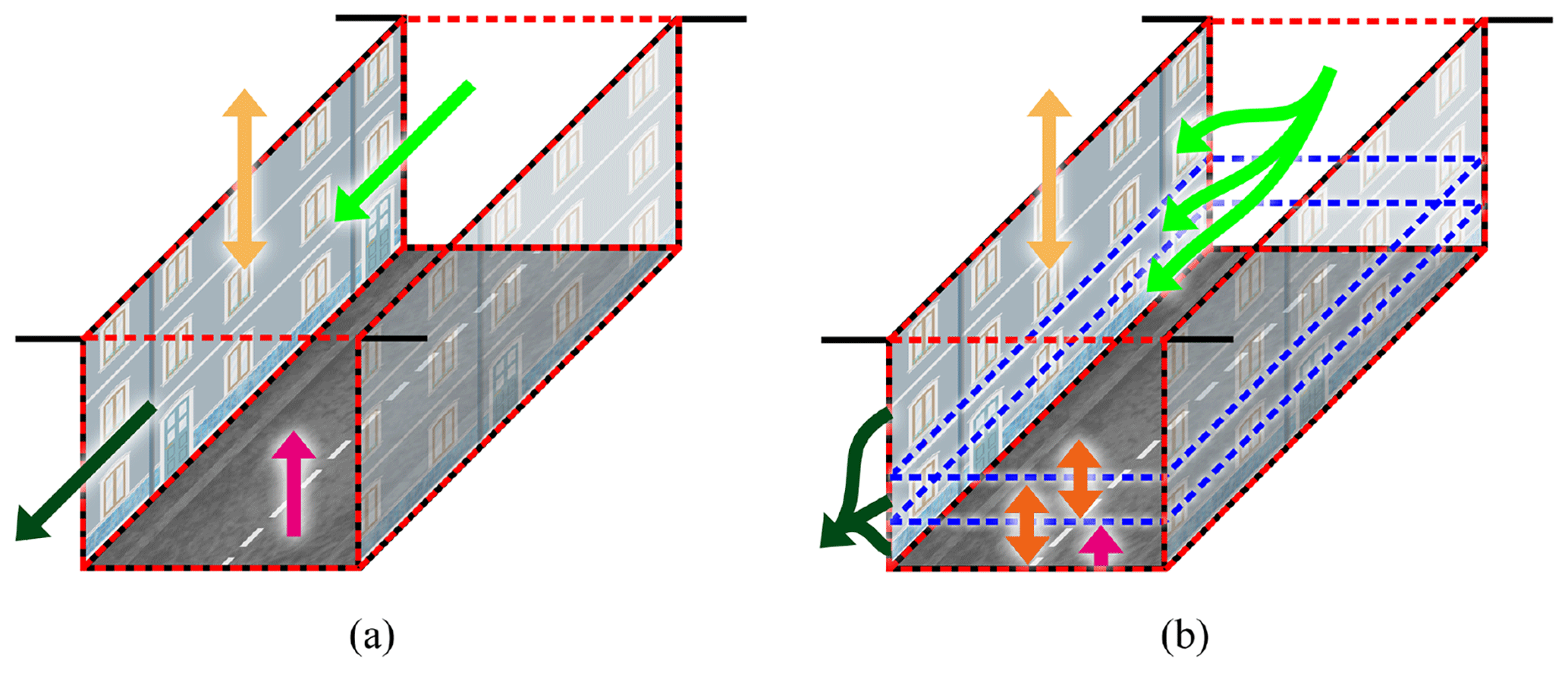
Figure 1 Representation of the processes in the homogeneous version (a) and the heterogeneous version (b) of MUNICH. The dotted red lines represent the street volume. In (a), the street canopy is represented by a single volume, whereas in (b), it is divided into three subvolumes delimited by the dotted blue lines. The rose arrows represent the traffic emissions (including brake, tyre, and road wear), the light-green arrows represent the fluxes entering the street via the upwind intersection, and the dark-green arrows represent the fluxes leaving the street via the downwind intersection. The yellow arrows symbolize the vertical turbulent exchanges with the background, and in (b), the orange arrows symbolize the vertical exchanges among the subvolumes.

In order to solve the evolution equation of the street concentrations C_str, a first-order operator splitting between transport and chemistry is performed:

$$\begin{array}{}\text{(1)}& {\displaystyle \frac{\mathrm{d}{C}_{\text{str}}}{\mathrm{d}t}}={\left.{\displaystyle \frac{\mathrm{d}{C}_{\text{str}}}{\mathrm{d}t}}\right|}_{\text{tr}}+{\left.{\displaystyle \frac{\mathrm{d}{C}_{\text{str}}}{\mathrm{d}t}}\right|}_{\text{ch}}.\end{array}$$

The transport term includes advection from one street to another and vertical transport between the street and the background above it. The chemistry includes gas-phase chemistry, as well as aerosol dynamics (coagulation, condensation, and evaporation). As deposition and resuspension processes have minor effects compared to transport and chemistry (Lugon et al., 2021b; Kim et al., 2022), they are omitted in the rest of this study.

2.1 Homogeneous approach

Using a box model approach, the concentrations are assumed to be homogeneous in the whole street volume, and the effects of the processes on the concentrations are represented by the following equation:

$$\begin{array}{}\text{(2)}& {\left.{\displaystyle \frac{\mathrm{d}{C}_{\text{str}}}{\mathrm{d}t}}\right|}_{\text{tr}}={\displaystyle \frac{\mathrm{1}}{V}}\left(Q_{\text{em}}+Q_{\text{inflow}}+Q_{\text{outflow}}+Q_{\text{vert}}\right),\end{array}$$

where V is the volume of the rectangular cuboid street, Q_em is the traffic emission flux, Q_inflow is the flux entering the street via the upwind intersection, Q_outflow is the flux leaving the street via the downwind intersection, and Q_vert is the vertical turbulent flux between the background and the street.

The street volume is defined as V=HWL, with H being the average building height over the street segment, W being the mean street width, and L being its length. MUNICH considers it to be that buildings on each side of the street are continuous, thus not representing inflow and/or outflow that could be induced by gaps in the buildings. The inflow term Q_inflow is obtained from the computation of the fluxes at the upwind intersection (Kim et al., 2018; Soulhac et al., 2009) (see Sect. 5 for a brief description). The outflow term Q_outflow is expressed as follows:

$$\begin{array}{}\text{(3)}& Q_{\text{outflow}}=HW{u}_{\text{str}}{C}_{\text{str}},\end{array}$$

with u_str being the mean horizontal wind speed in the street.

The vertical turbulent flux Q_vert between the street and the overlying atmosphere is

$$\begin{array}{}\text{(4)}& Q_{\text{vert}}=q_{\text{vert}}WL{\displaystyle \frac{\left(C_{\text{str}}-C_{\text{bkgd}}\right)}{H}},\end{array}$$

with q_vert being the vertical transfer coefficient and C_bkgd being the background concentration.

The vertical transfer coefficient and the horizontal wind speed are the key parameters representing the dispersion of concentrations. As their formulation differs between the homogeneous and the heterogeneous versions of MUNICH, they are now detailed.

2.1.1 Vertical transfer coefficient for turbulent flux

Three parameterizations are implemented in MUNICH to determine the vertical transfer coefficient q_vert between the street and the overlying atmosphere (Maison et al., 2022). However, currently, only the parameterization adapted from Wang (2014) is designed to provide vertical profiles for both wind speed and mixing length within the street. We therefore limit our analysis to the latter.

In MUNICH-homo, the vertical transfer coefficient at the roof level is expressed as follows:

$$\begin{array}{}\text{(5)}& q_{\text{vert}}={\mathit{\sigma }}_{\mathrm{w}}{l}_{\mathrm{m}}(z=H)\text{ with }{l}_{\mathrm{m}}\left(z\right)={\displaystyle \frac{\mathit{\kappa }z{l}_{\mathrm{c}}}{l_{\mathrm{c}}+\mathit{\kappa }z}},\end{array}$$

where σ_w is the standard deviation of the vertical wind velocity at roof level, and l_m is the mixing length defined as a harmonic mean between two length scales (Coceal and Belcher, 2004), namely (i) κz, with the Von Kármán constant (κ=0.42), and (ii) l_c, which is a characteristic length of the street chosen to be equal to 0.5W (Maison et al., 2022).

2.1.2 Mean horizontal wind speed in the street

As for the calculation of the vertical transfer coefficient, three parameterizations are proposed in MUNICH to determine the mean horizontal wind speed in the street (Maison et al., 2022). In the Wang parameterization, the mean horizontal wind speed in the street u_str is equal to

$$\begin{array}{}\text{(6)}& \begin{array}{rl}{u}_{\text{str}}& ={\displaystyle \frac{\mathrm{1}}{H-z_{\mathrm{0}s}}}\underset{z_{\mathrm{0}s}}{\overset{H}{\int }}{u}_Y\left(z\right)\mathrm{d}z\\ & ={\displaystyle \frac{u_H\left|\cos \right(\mathit{\phi }\left)\right|}{(H-z_{\mathrm{0}s})}}\underset{z_{\mathrm{0}s}}{\overset{H}{\int }}\left[J_{\mathrm{1}}{I}_{\mathrm{0}}\left(g\right(z\left)\right)+J_{\mathrm{2}}{K}_{\mathrm{0}}\left(g\right(z\left)\right)\right]\mathrm{d}z,\end{array}\end{array}$$

with $u_H\left|\cos \right(\mathit{\phi }\left)\right|$ being the wind speed at roof level in the direction of the street and z_0s being the wall and ground roughness length in the street (fixed to 0.01 m). I₀ and K₀ are the first- and second-kind modified Bessel functions of order 0. J₁ and J₂ are integration coefficients equal to

$$\begin{array}{}\text{(7)}& \begin{array}{rl}& J_{\mathrm{1}}={\displaystyle \frac{\mathrm{1}}{I_{\mathrm{0}}\left(g\right(H\left)\right)-I_{\mathrm{0}}\left(g\right(z_{\mathrm{0}s}\left)\right)K_{\mathrm{0}}\left(g\right(H\left)\right)/K_{\mathrm{0}}\left(g\right(z_{\mathrm{0}s}\left)\right)}}\text{ and}\\ & J_{\mathrm{2}}=-{\displaystyle \frac{J_{\mathrm{1}}{I}_{\mathrm{0}}\left(g\right(z_{\mathrm{0}s}\left)\right)}{K_{\mathrm{0}}\left(g\right(z_{\mathrm{0}s}\left)\right)}}.\end{array}\end{array}$$

The function g(z) is calculated as follows:

$$\begin{array}{}\text{(8)}& g\left(z\right)=\mathrm{2}\sqrt{C_B{a}_r{\displaystyle \frac{z}{l_{\mathrm{m}}\left(H\right)}}},\end{array}$$

with $a_r=H/W$ being the aspect ratio of the street and C_B being a coefficient that is dependent on the wind angle with the street and the aspect ratio (Maison et al., 2022).

2.2 Heterogeneous approach

In MUNICH-hete, the street is divided into three vertical levels to limit the artificial dilution of the traffic emissions and the concentrations in the whole street volume (see Figs. 1b and 2). Levels are ordered from the ground to the top of the street. The first level (i=1) contains the traffic emissions. The thickness h₁ is taken as 2 m, which corresponds to a zone where the traffic producing turbulence mixes and dilutes traffic emissions (Solazzo et al., 2008). This traffic-induced turbulence is not explicitly considered in the model. The second-level (i=2) thickness h₂ is also of 2 m. It acts as a buffer zone between the first level, where traffic emissions are, and the third level, where exchanges with the background take place. Starting at 4 m, the third level (i=3) goes to the roof level ($h_{\mathrm{3}}=(H-\mathrm{4})$ m). The minimum street height considered in the model is set at 6 m. The three levels of the heterogeneous version are referred to as MUNICH-hete-l1, MUNICH-hete-l2, and MUNICH-hete-l3. Each level i is thus associated with a specific volume V_i, and the evolution equations may be written as follows:

$$\begin{array}{}\text{(9)}& \begin{array}{rl}& {\left.{\displaystyle \frac{\mathrm{d}{C}_{\text{str}}^i}{\mathrm{d}t}}\right|}_{\text{tr}}=\\ & {\displaystyle \frac{\mathrm{1}}{V_i}}(Q_{\text{em}}^i+Q_{\text{inflow}}^i+Q_{\text{outflow}}^i+Q_{\text{vert}}^{i,i+\mathrm{1}}+Q_{\text{vert}}^{i-\mathrm{1},i}),\end{array}\end{array}$$

where $Q_{\text{em}}^i$ is the traffic emission flux (only in the first level (i=1)), $Q_{\text{inflow}}^i$ is the flux entering the level via the upwind intersection, $Q_{\text{outflow}}^i$ is the flux leaving the level via the downwind intersection, $Q_{\text{vert}}^{i,i+\mathrm{1}}$ is the vertical turbulent flux between the levels i and i+1 (for i=3, it is exchanged with the background), and $Q_{\text{vert}}^{i-\mathrm{1},i}$ is the vertical turbulent flux between the levels i−1 and i (equal to zero if i=1).

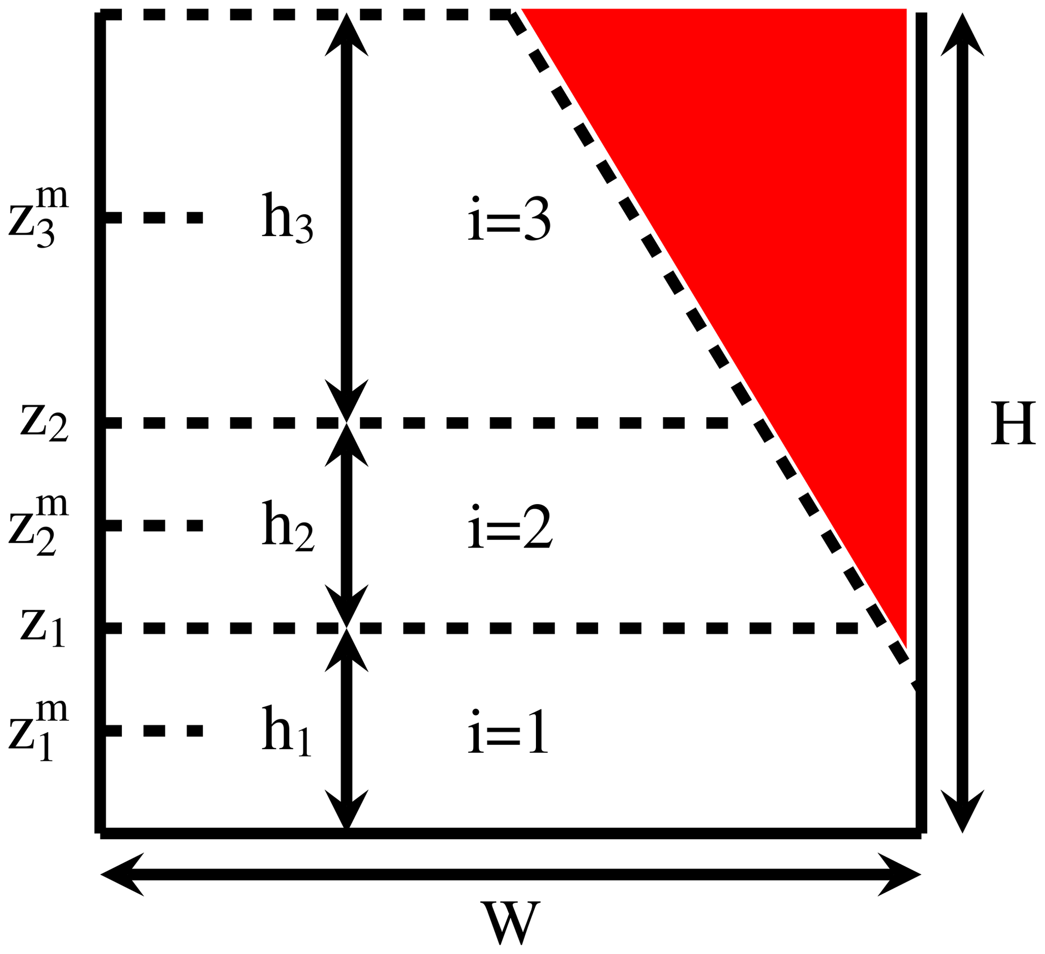
Figure 2 Schematic of the discretization in MUNICH-hete. The red triangle represents the ventilation zone that is present under specific conditions, and the white trapeze represents the recirculation zone. $z_i^{\mathrm{m}}$ is the middle height of level i.

Note that more than three vertical levels could be defined in MUNICH-hete as the vertical variations within the streets of winds and mixing lengths are parameterized when discretizing the streets. However, the first vertical level at the bottom of the street should not be too thin because of mixing due to traffic turbulence. A minimum height for the first layer of 1.5 m seems reasonable.

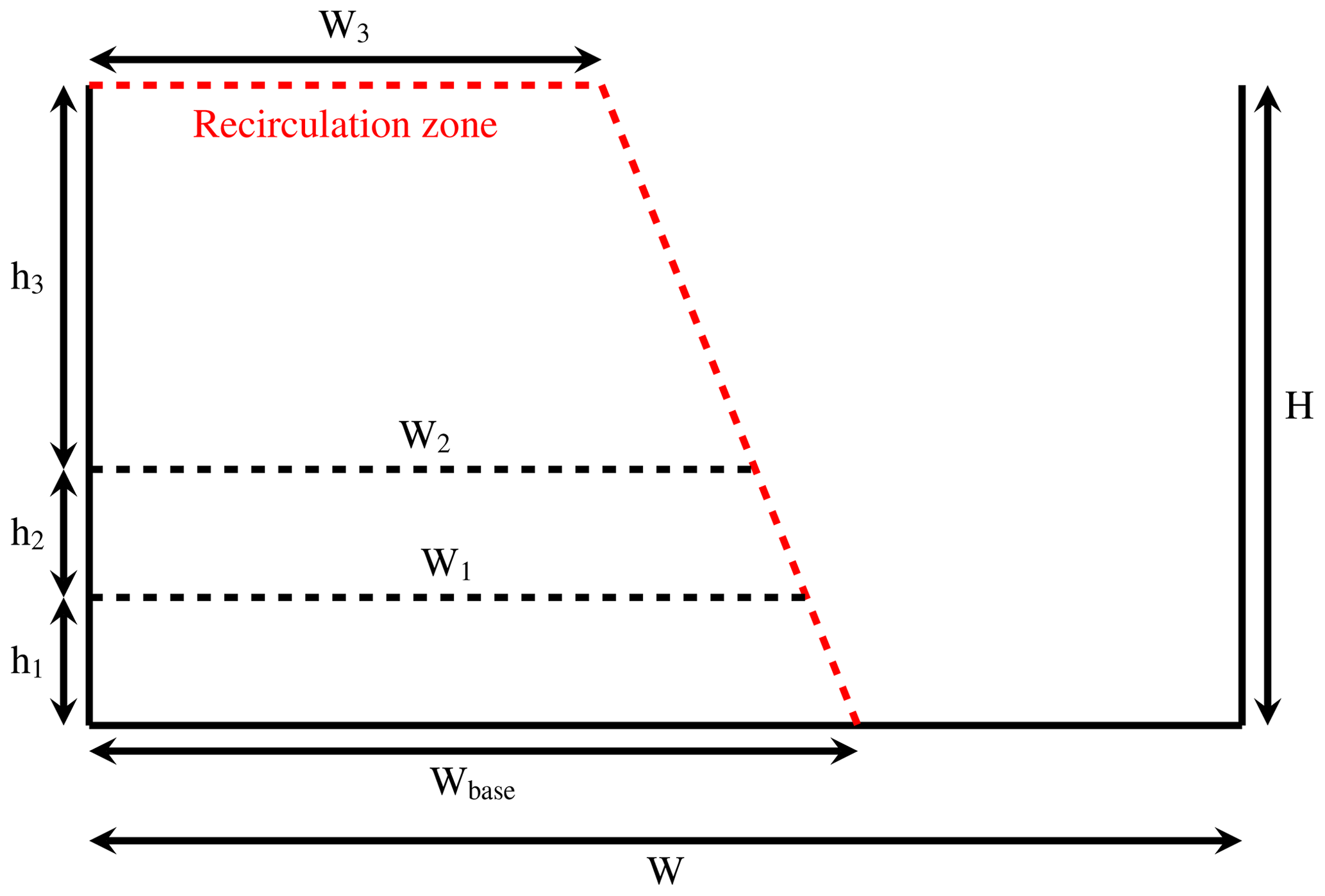
In OSPM, the flow that develops into a vortex in the street between buildings is represented by a recirculation zone. It occupies the whole street volume for narrow streets, and it has the shape of a trapeze for wider streets (Berkowicz et al., 1997; Berkowicz, 2000b; Ottosen et al., 2015). When the recirculation zone does not occupy the whole street volume, there is a ventilation zone (see Fig. 2) where concentrations of pollutants emitted by traffic are usually lower than in the recirculation zone. In MUNICH-homo, the recirculation zone is not explicit, whatever the street ratio (H/W) is. In MUNICH-hete, the volume of the recirculation zone is computed as in OSPM, as detailed in Appendix A. For now, concentrations in the ventilation zone are considered to be homogeneous and equal to the background concentrations, i.e. concentrations above the street. The ventilation zone is thus taken into account when it is not affected by traffic emissions. In practice, this means that the width of the trapeze base can only be equal to or larger than the width W of the street (see Appendix A). The width W_i of the level i can thus be inferior to the width W of the street, reducing the level volume (see Fig. 2). Appendix A presents the algorithm implemented in MUNICH-hete to consider the volume reduction of the ventilation zone. Further work is needed to differentiate the two zones for cases where the ventilation zone develops further into the street.

To quantify mass transfer through the intersections, the fluxes are assumed to be vertically homogeneous and remain determined as proposed by Soulhac et al. (2009) as the shapes of the intersections may differ from one to another, and turbulence is not quantified. The flux Q_inflow entering the street is assumed to be the same for each vertical level. The flux Q_outflow leaving a street is a surface-weighted average of the fluxes leaving each vertical level of the street:

$$\begin{array}{}\text{(10)}& Q_{\text{outflow}}=\sum _{i=\mathrm{1}}^{i=\mathrm{3}}{Q}_{\text{outflow}}^i=\sum _{i=\mathrm{1}}^{i=\mathrm{3}}{S}_i^{\mathrm{v}}{u}_i{C}_{\text{str}}^i,\end{array}$$

with $S_i^{\mathrm{v}}$ being the vertical surface of the level i, as presented in Appendix A, and u_i being the mean horizontal wind speed of the level i (see Sect. 2.2.2).

2.2.1 Vertical turbulent fluxes

To compute the vertical turbulent transfer $Q_{\text{vert}}^{i,i+\mathrm{1}}$ at the interface of the vertical levels i and i+1, Eq. (4) is modified to represent the vertical exchanges between the levels i and i+1:

$$\begin{array}{}\text{(11)}& Q_{\text{vert}}^{i,i+\mathrm{1}}=q_{\text{vert}}^i{W}_{i}L{\displaystyle \frac{\left(C_i-C_{i+\mathrm{1}}\right)}{\mathrm{\Delta }{z}_i^{\mathrm{m}}}},\end{array}$$

where C_i and C_i+1 are the concentrations in the levels i and i+1 respectively; W_i is the width of the level i that is inferior or equal to the width W of the street; and $\mathrm{\Delta }{z}_i^{\mathrm{m}}$ is the difference in altitude between the middles of the levels i+1 and i, which are as noted $z_{\mathrm{1}}^{\mathrm{m}}$, $z_{\mathrm{2}}^{\mathrm{m}}$, and $z_{\mathrm{3}}^{\mathrm{m}}$ (see Fig. 2). For i=3, i.e. the highest level, $z_{i+\mathrm{1}}^{\mathrm{m}}$ is taken as the symmetrical of $z_{\mathrm{3}}^{\mathrm{m}}$ to the roof level and is noted as $z_{\text{bkgd}}^{\mathrm{m}}$. It gives an approximation of the volume that effectively exchanges with the third level.

Among the three parameterizations implemented in MUNICH to determine the vertical transfer coefficient q_vert, only the Wang parameterization is adapted to the discretization. It is thanks to its explicit vertical dependency and validity for a wide range of street canyon and wind characteristics (Maison et al., 2022). To compute the vertical turbulent transfer $Q_{\text{vert}}^{i,i+\mathrm{1}}$, the vertical transfer coefficient is taken at the height of the interface between the two vertical levels considered, and Eq. (5) is now written as follows:

$$\begin{array}{}\text{(12)}& q_{\text{vert}}^i={\mathit{\sigma }}_{\mathrm{w}}\mathit{\kappa }{z}_i{\displaystyle \frac{l_{\mathrm{c}}}{l_{\mathrm{c}}+\mathit{\kappa }{z}_i}},\end{array}$$

where z_i is the height of the interface between levels i and i+1. The influence of the atmospheric stability on vertical mixing is taken into account by modifying the standard deviation of the vertical wind velocity at roof level and thus the vertical transfer rate, depending on the length of Monin–Obukhov, as in MUNICH-homo.

By combining Eqs. (11) and (12), the vertical turbulent transfer $Q_{i,i+\mathrm{1}}$ can be written for each level as follows:

$$\begin{array}{}\text{(13)}& {\displaystyle }& {\displaystyle }{Q}_{\text{vert}}^{\mathrm{1},\mathrm{2}}={\mathit{\sigma }}_{\mathrm{w}}\mathit{\kappa }{z}_{\mathrm{1}}{\displaystyle \frac{l_{\mathrm{c}}}{l_{\mathrm{c}}+\mathit{\kappa }{z}_{\mathrm{1}}}}{W}_{i}L{\displaystyle \frac{C_{\mathrm{1}}-C_{\mathrm{2}}}{z_{\mathrm{2}}^{\mathrm{m}}-z_{\mathrm{1}}^{\mathrm{m}}}},\text{(14)}& {\displaystyle }& {\displaystyle }{Q}_{\text{vert}}^{\mathrm{2},\mathrm{3}}={\mathit{\sigma }}_{\mathrm{w}}\mathit{\kappa }{z}_{\mathrm{2}}{\displaystyle \frac{l_{\mathrm{c}}}{l_{\mathrm{c}}+\mathit{\kappa }{z}_{\mathrm{2}}}}{W}_{i}L{\displaystyle \frac{C_{\mathrm{2}}-C_{\mathrm{3}}}{z_{\mathrm{3}}^{\mathrm{m}}-z_{\mathrm{2}}^{\mathrm{m}}}},\text{(15)}& {\displaystyle }& {\displaystyle }{Q}_{\text{vert}}^{\mathrm{3},\text{bkgd}}={\mathit{\sigma }}_{\mathrm{w}}\mathit{\kappa }H{\displaystyle \frac{l_{\mathrm{c}}}{l_{\mathrm{c}}+\mathit{\kappa }H}}{W}_{i}L{\displaystyle \frac{C_{\mathrm{3}}-C_{\text{bkgd}}}{z_{\text{bkgd}}^{\mathrm{m}}-z_{\mathrm{3}}^{\mathrm{m}}}},\end{array}$$

with C₁, C₂, C₃, and C_bkgd being the concentrations of the three levels and the background respectively.

2.2.2 Mean horizontal wind speed in the street

As for the vertical turbulent flux, the Wang parameterization is preferred among the three parameterizations available in MUNICH to compute the mean horizontal wind speeds in the street. This is thanks to its explicit vertical dependency and the no-slip condition at the ground that is always satisfied ($u(z=\mathrm{0})=\mathrm{0}$) (Maison et al., 2022). Therefore, the mean horizontal wind speed can be computed at each level in the street by modifying Eq. (6) to integrate vertically between the level heights:

$$\begin{array}{}\text{(16)}& {\displaystyle }& {\displaystyle }{u}_{\mathrm{1}}={\displaystyle \frac{\mathrm{1}}{z_{\mathrm{1}}-z_{\mathrm{0}s}}}{\displaystyle }\underset{z_{\mathrm{0}s}}{\overset{z_{\mathrm{1}}}{\int }}{u}_Y\left(z\right)\mathrm{d}z,\text{(17)}& {\displaystyle }& {\displaystyle }{u}_{\mathrm{2}}={\displaystyle \frac{\mathrm{1}}{z_{\mathrm{2}}-z_{\mathrm{1}}}}{\displaystyle }\underset{z_{\mathrm{1}}}{\overset{z_{\mathrm{2}}}{\int }}{u}_Y\left(z\right)\mathrm{d}z,\text{(18)}& {\displaystyle }& {\displaystyle }{u}_{\mathrm{3}}={\displaystyle \frac{\mathrm{1}}{H-z_{\mathrm{2}}}}{\displaystyle }\underset{z_{\mathrm{2}}}{\overset{H}{\int }}{u}_Y\left(z\right)\mathrm{d}z,\end{array}$$

with z₁ and z₂ being the limits of the first two levels, as presented in Fig. 2.

3 Application to street networks in Copenhagen with comparison to OSPM

This section presents two applications of MUNICH-hete to assess its capabilities compared to MUNICH-homo and OSPM. Simulations are performed over the year 2019 to generate hourly concentrations for two street networks in Copenhagen, Denmark. The first street network is centred around H. C. Andersens Boulevard, and the second is centred around Jagtvej street. They are respectively named HCAB and JGTV in the following. These street networks have been selected as observational data of CO, NO₂, NO_x, and O₃ are available for HCAB, and observational data of NO₂ and NO_x are available for JGTV, both over the whole year. OSPM simulations were also performed to compare model performances. As OSPM does not represent air fluxes at intersections, OSPM simulations are performed only for the streets where there are observations. Thanks to its coupled approach of a Gaussian plume model and a box model, OSPM is able to calculate concentrations on the two sides of the street (Berkowicz et al., 1997; Berkowicz, 2000b; Ottosen et al., 2015). Two receptors are used to compare with the observed concentrations on each side of the street: OSPM-R1 and OSPM-R2. The height of the receptors is taken as 2 m to correspond roughly to the height at which observations were performed. They are compared to the concentrations simulated at the first two levels of MUNICH-hete, which are representative of the concentrations at 1 and 3 m.

MUNICH and OSPM use the same input data to estimate the street concentrations. The meteorological parameters originate from simulations performed with the Weather Research and Forecasting model (WRF,  Skamarock et al., 2008). The background concentrations are simulated using the Urban Background Model (UBM,  Berkowicz, 2000a), which is “a multiple source model that applies a Gaussian approach for horizontal dispersion and a linear approach for vertical dispersion up to the boundary layer” (Jensen et al., 2016). Traffic emissions are generated using the procedure implemented in the local-scale Gaussian air pollution model OML-Highway (Olesen et al., 2015), allowing for precise information for each street segment. Traffic data (average daily traffic, travel speed, and share of heavy-duty vehicles) are used to generate emissions by use of the European emission model COPERT IV. Traffic emissions include exhaust emissions of gases and particles and non-exhaust emissions of particles. Non-exhaust emissions consist of brake, tyre, and road wear. The street parameters (building height and street width) used in MUNICH originate from the OSPM setups.

OSPM represents NO₂ and O₃ chemical transformations using a system of two reactions (Berkowicz et al., 1997; Berkowicz, 2000b). The first one describes the production of NO₂ due to the reaction of NO with O₃, and the second one describes the photodissociation of NO₂ that leads to the reproduction of NO and O₃. For a fair comparison, MUNICH is configured to run with a simple chemistry scheme, the Leighton photostationary state for O₃ (Leighton, 1961; Kim et al., 2018):

$$\begin{array}{}\text{(R1)}& {\displaystyle }{\mathrm{NO}}_{\mathrm{2}}+h\mathit{\nu }& {\displaystyle }\to \mathrm{NO}+\mathrm{O}{(}^{\mathrm{3}}\mathrm{P}),\text{(R2)}& {\displaystyle }\mathrm{O}{(}^{\mathrm{3}}\mathrm{P})+{\mathrm{O}}_{\mathrm{2}}+\mathrm{M}& {\displaystyle }\to {\mathrm{O}}_{\mathrm{3}}+\mathrm{M},\text{(R3)}& {\displaystyle }\mathrm{NO}+{\mathrm{O}}_{\mathrm{3}}& {\displaystyle }\to {\mathrm{NO}}_{\mathrm{2}}+{\mathrm{O}}_{\mathrm{2}}.\end{array}$$

3.1 H. C. Andersens Boulevard

H. C. Andersens Boulevard is a wide, densely trafficked boulevard, with an aspect ratio $a_r=H/W$ of about 0.2 (H=9.9 m, W=50 m). It is open on one side with trees instead of buildings. This configuration can be represented in OSPM. However, in MUNICH, a mean building height is defined for each street. Here, it is estimated by averaging the building and the tree heights. The simulated street network is composed of 86 street segments centred around the street where the observation station is located (see brown cross in Fig. 4). Figure 3 presents the monthly averaged concentrations of CO and NO₂ from the OSPM and MUNICH simulations compared to observations. Appendix C contains monthly averaged concentrations of NO_x and O₃ and statistical indicators of the comparison for all four pollutants.

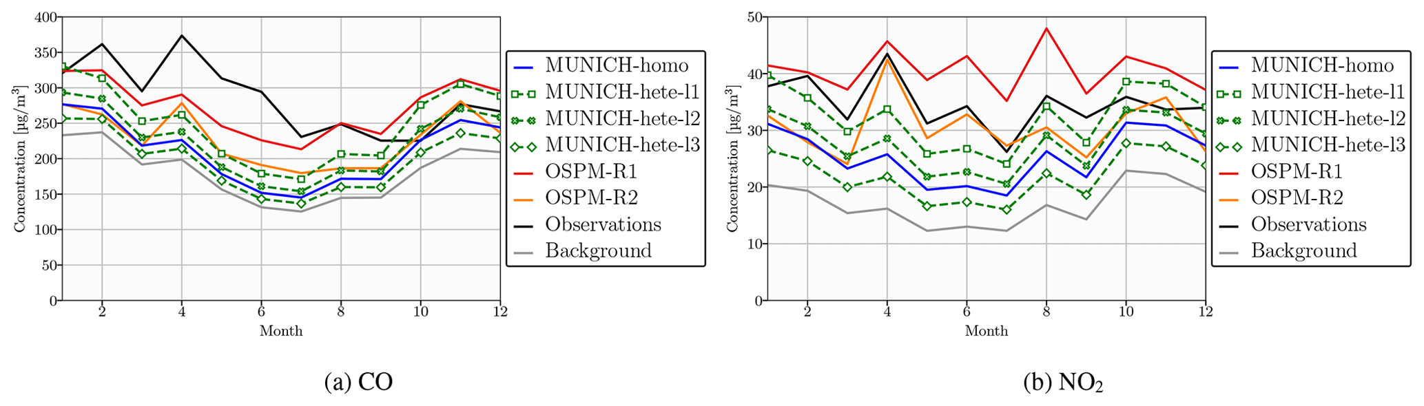
Figure 3 Monthly averaged concentrations (in µg m⁻³) of CO (a) and NO₂ (b) at HCAB monitoring station. The solid blue line represents the homogeneous version of MUNICH. The three dashed green lines represents the three levels of the heterogeneous version of MUNICH – the lowest level (l1) is shown with square markers, the intermediate level (l2) is shown with crossed markers, and the top level (l3) is shown with diamond markers. The solid red line represents the OSPM receptor that is close to the measurement station, and the solid orange line represents the second OSPM receptor located on the other side of the street. The observations are in solid black, and the background concentrations are in solid grey.

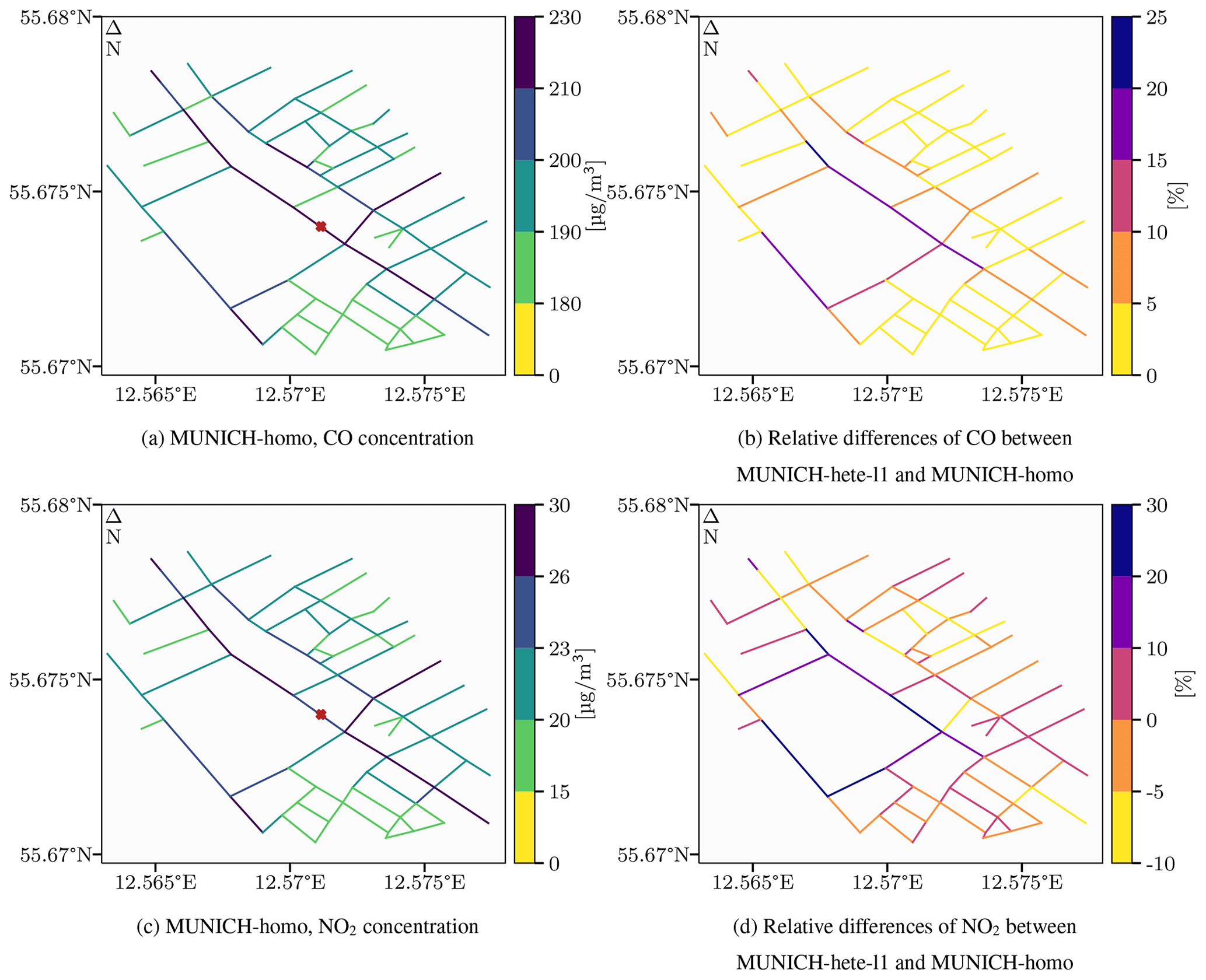
Figure 4 CO and NO₂ time-averaged concentrations (in µg m⁻³) for MUNICH-homo are shown in the upper- and lower-left panels (a, c) respectively for the HCAB street network. Relative differences (in %) between the first level of MUNICH-hete and MUNICH-homo for CO and NO₂ are shown in the upper- and lower-right panels (b, d) respectively for the HCAB street network. A positive relative difference indicates higher concentrations for MUNICH-hete. The brown cross in panels (a) and (c) represents the position of the measurement station.

OSPM-R1 is the receptor that is close to the measurement station and is thus better suited to be compared to observations. Differences in the concentrations between OSPM-R1 and OSPM-R2 highlight the importance of taking into account the horizontal heterogeneities in the street. Observations lie between the concentrations simulated at the two receptors, except in the case of CO, for which OSPM slightly underestimates concentrations in the first half of the year. This underestimation could be linked to underestimation of sources other than traffic, e.g. biomass burning, at the regional scale but could also be due to the absence of volatile organic compounds in the simulation. Overall, the concentrations are well estimated with OSPM, with errors between 26 % and 33 % for CO and between 34 % and 46 % for NO₂.

For CO, NO₂, and NO_x, which are emitted by traffic in the bottom of the street, the concentrations are higher in the first level, MUNICH-hete-l1, near the bottom and are lower in the third level, MUNICH-hete-l3, near the roof level. For O₃, the opposite behaviour is observed as it is mainly imported by the atmosphere above the street, and it is titrated by NO near the ground. The first two levels, MUNICH-hete-l1 and MUNICH-hete-l2, have higher concentrations of CO, NO₂, and NO_x than munich-homo, thus improving the comparison to observations and OSPM concentrations. For CO, the error is improved from 36 % in MUNICH-homo to 28 % in MUNICH-hete-l1, and for NO₂, it is improved from 48 % in MUNICH-homo to 35 % in MUNICH-hete-l1. Although the concentrations of NO₂ and CO are underestimated in MUNICH-homo compared to observations, they are well modelled in the first level, MUNICH-hete-l1, with low errors and biases (see Appendix C). For CO, the concentrations simulated in the first level, MUNICH-hete-l1, lie between the two OSPM receptors for most of the year. This is the case for NO₂ as well, except between April and August, when NO₂ concentrations are underestimated in MUNICH-hete compared to observations and OSPM concentrations. The formation of NO₂ in the lower levels (see Reaction R3) could be limited with the current model setup because volatile organic compounds are not taken into account in the Danish cases. However, they may participate in O₃ and NO₂ formation through HO₂ and RO₂ radicals (Atkinson, 2000; Kwak and Baik, 2012; Zhong et al., 2017; Dai et al., 2021). Furthermore, the vertical discretization is coarse, limiting O₃ transport deep into the street.

Over the whole street network, as presented in Fig. 4, the differences between the concentrations simulated in the first vertical level of MUNICH-hete and those simulated in MUNICH-homo vary. For wide streets and avenues with dense traffic, the concentrations are higher in MUNICH-hete-l1 than in MUNICH-homo, with an increase of up to 23 % for CO and 30 % for NO₂. This increase is lower in more narrow and less frequented streets. Although the concentrations in MUNICH-hete-l1 are always higher than those in MUNICH-homo for CO, for NO₂, in narrow streets, the concentrations are lower in MUNICH-hete-l1. These lower NO₂ concentrations are probably related to the limited transport of O₃ from the background to the bottom of the street, limiting the titration of NO.

3.2 Jagtvej

Jagtvej is a conventional street canyon with an aspect ratio of about 0.8 (H=20.3 m, W=26.2 m). The simulated street network is composed of 265 street segments centred around the street where the observation station is located (see brown cross in Fig. 6). The monthly averaged concentrations of CO and NO₂ from the OSPM and MUNICH simulations compared to observations for NO₂ only are presented in Fig. 5. Appendix D contains monthly averaged concentrations of NO_x and O₃ and statistical indicators of the comparison for NO₂ and NO_x.

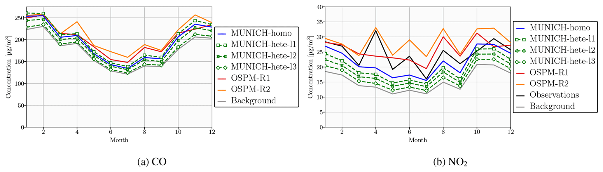
Figure 5 Monthly averaged concentrations (in µg m⁻³) of CO (a) and NO₂ (b) at JGTV monitoring station. The solid blue line represents the homogeneous version of MUNICH. The three dashed green lines represent the three levels of the heterogeneous version of MUNICH – the lowest level (l1) is shown with square markers, the intermediate level (l2) is shown with crossed markers, and the top level (l3) is shown with diamond markers. The solid orange line represents the OSPM receptor that is close to the measurement station, and the solid red line represents the second OSPM receptor located on the other side of the street. The observations (only available for NO₂) are in solid black, and the background concentrations are in solid grey.

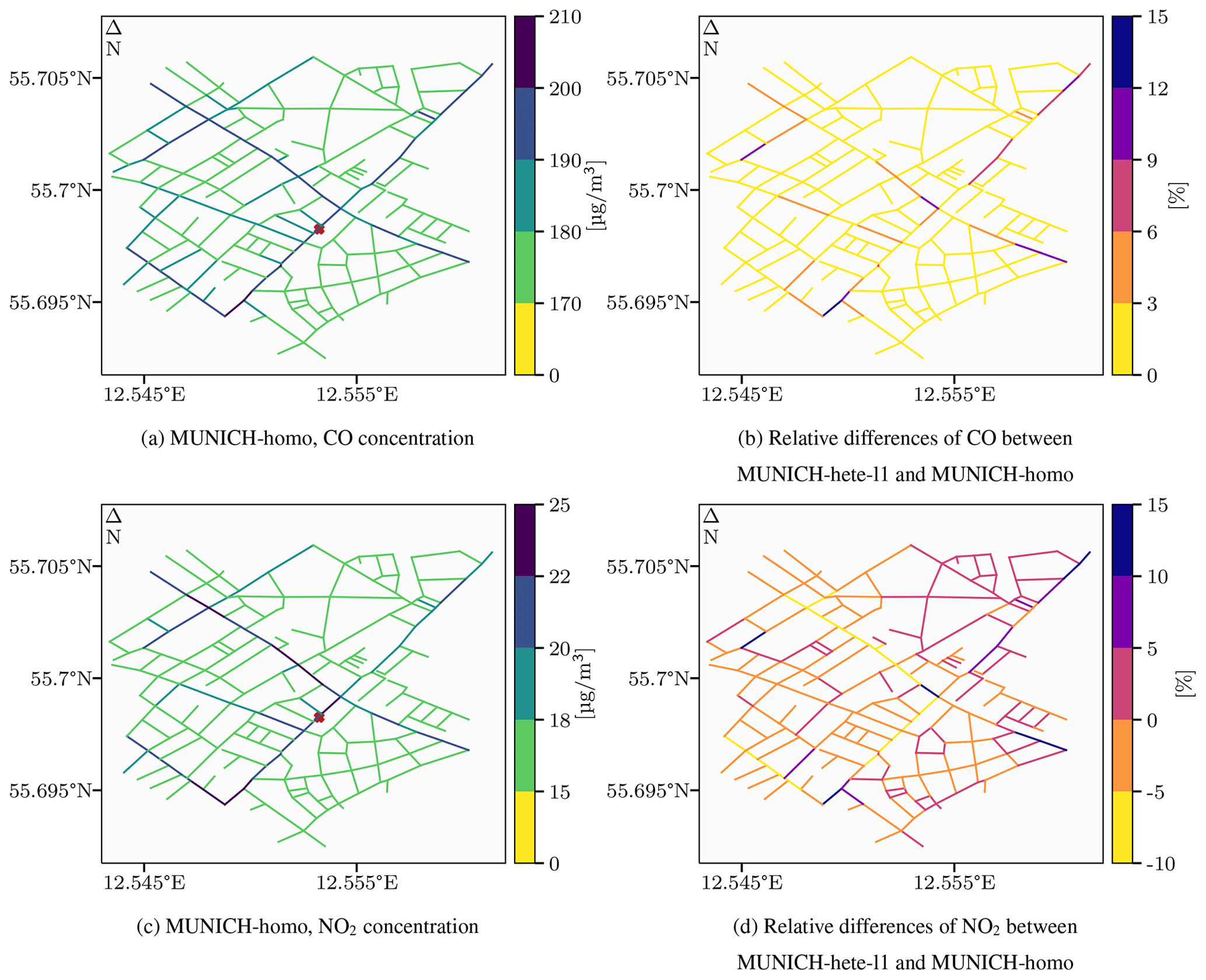
Figure 6 CO and NO₂ time-averaged concentrations (in µg m⁻³) for MUNICH-homo are shown in the upper- and lower-left panels (a, c) respectively for the JGTV street network. Relative differences (in %) between the first level of MUNICH-hete and MUNICH-homo for CO and NO₂ are shown in the upper- and lower-right panels (b, d) respectively for JGTV. A positive relative difference indicates higher concentrations for MUNICH-hete. The brown cross in panels (a) and (c) represents the position of the measurement station.

OSPM-R2 is the receptor that is close to the measurement station and is thus better suited to be compared to observations. The differences between the concentrations of the two OSPM receptors are lower in JGTV than in HCAB (see Fig. 3). JGTV is narrower, with higher buildings on both sides, thus limiting the ventilation zone and the penetration into the street of background concentrations that would reduce the concentrations at the downwind receptor. OSPM tends to slightly overestimate NO₂ and NO_x concentrations (with errors between 41 % and 53 % and between 42 % and 63 % respectively).

Concentrations from the homogeneous version of MUNICH are close to OSPM concentrations for CO. They are lower than OSPM concentrations for NO₂, but they compare well to observations, with a bias of −3 % and an error of 46 %. These lower NO₂ concentrations are linked to lower NO_x concentrations (with a bias of −19 % compared to observations and an error of 53 %). As for HCAB, the MUNICH-hete concentrations decrease from the bottom to the top of the street. For CO and NO_x, only the first level has concentrations higher than MUNICH-homo, while for NO₂, all three levels have concentrations lower than MUNICH-homo. O₃ concentrations are also higher for the three levels (see Fig. D1). The NO_x concentrations of MUNICH-hete-l1 compare slightly better to observations than MUNICH-homo, while MUNICH-homo is slightly better for NO₂. However, the statistics of the two models are quite close (Appendix D).

Conclusions are similar for the whole street network (see Fig. 6). The CO concentrations are slightly higher in the first level of MUNICH-hete than in MUNICH-homo. However, NO₂ concentrations at the bottom of the street in the first level of MUNICH-hete tend to be lower than in MUNICH-homo. In some specific street segments of the network, the differences in the concentrations for both CO and NO₂ are higher in MUNICH-hete-l1 than in MUNICH-homo. This is due to a mix of different traffic emissions and street morphologies which favour the transport of pollutants.

4 Application to a street network in greater Paris

The impacts of the discretization on gas and particle concentrations are evaluated over the street network near Paris, France, which was used to validate MUNICH v2.0 (Kim et al., 2022) and in several sensitivity studies (Lugon et al., 2021b; Sarica et al., 2022, 2023b). The street network represents a district of Le Perreux-sur-Marne, a suburb 13 km east of Paris, France. It is composed of 577 street segments (see Fig. 8). The street parameters (building height and street width) were obtained from the BD TOPO database (https://geoservices.ign.fr/bdtopo, last access: 12 September 2023). Simulations were performed from 22 March to 15 June 2014 to generate hourly concentrations with input data (emissions, including exhaust emissions and brake, tyre, and road wear; meteorological parameters; and background concentrations) from the reference simulation SCN0 of Sarica et al. (2023b). For this case, MUNICH is coupled to SSH-aerosol (Sartelet et al., 2020) to represent gas-phase chemistry and aerosol dynamics. Observational data are available for the whole simulation period for NO₂, NO_x, PM_2.5, PM₁₀, and black carbon (BC) for a segment of Boulevard d'Alsace Lorraine (see brown cross in Fig. 8). The simulations were performed at a height of about 2 m, and they are thus to be compared to the concentrations of the first two levels (i=1 and i=2) of MUNICH-hete. The segment has an aspect ratio of about 0.3 (H=8.6 m, W=26 m).

The average daily profiles of NO_x and PM₁₀ concentrations are shown in Fig. 7, and NO, NO₂, and the statistical indicators are shown in Appendix E1. As in the Danish streets, for pollutants emitted by traffic, the concentrations are higher in MUNICH-hete at the bottom of the street, decreasing to the roof level. The concentrations of PM₁₀, NO₂, NO_x, and BC are higher on average by 12 %, 21 %, 40 %, and 30 % respectively in MUNICH-hete-l1 than in MUNICH-homo. The lower concentration difference for PM₁₀ than for the other compounds reflects the fact that non-traffic sources are more important for PM₁₀, and inversely, they are small for BC. Despite the higher concentrations in MUNICH-hete-l1, BC concentrations remain strongly underestimated compared to observations, in agreement with the CFD simulations of Lin et al. (2023). For PM₁₀, NO₂, and NO_x, the concentrations compare well to observations; e.g. the error is 33 % for NO₂ and 37 % for PM₁₀, with slightly better statistics using MUNICH-hete-l1 than MUNICH-homo. For all pollutants, the concentrations of the intermediate level (i=2) are very close to the concentrations of MUNICH-homo. This is due to a mixture of different parameters such as street morphology and dispersion conditions over the simulated period.

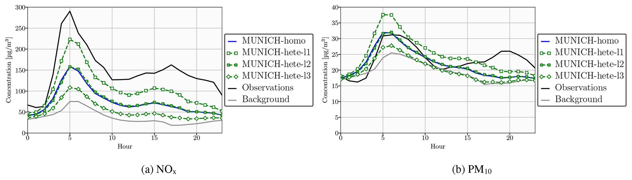
Figure 7 Average daily profile of the concentrations of NO_x (a) and PM₁₀ (b) over the simulation period at the Boulevard d'Alsace Lorraine monitoring station. The solid blue line represents the homogeneous version of MUNICH. The three dashed green lines represent the three levels of the heterogeneous version of MUNICH – the lowest level (l1) is shown with square markers, the intermediate level (l2) is shown with crossed markers, and the top level (l3) is shown with diamond markers. The observations are in solid black, and the background concentrations are in solid grey.

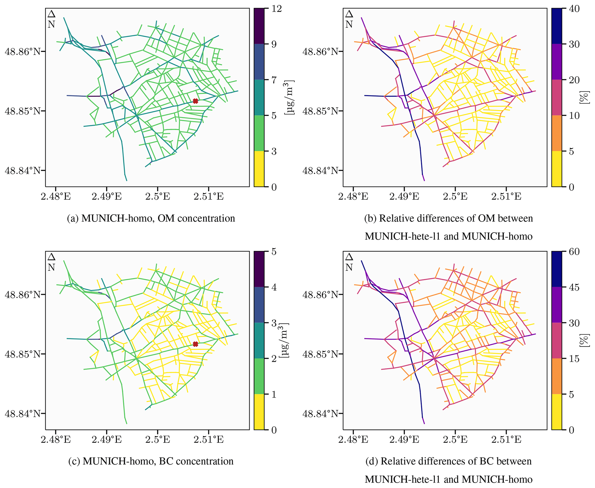
Figure 8 OM and BC time-averaged concentrations (in µg m⁻³) for MUNICH-homo are shown in the upper- and lower-left panels (a, c) respectively for the district of Le Perreux-sur-Marne. Relative differences (in %) between the first level of MUNICH-hete and MUNICH-homo for OM and BC are shown in the upper- and lower-right panels (b, d) respectively for the district of Le Perreux-sur-Marne. A positive relative difference indicates higher concentrations for MUNICH-hete. The brown cross in panels (a) and (c) represents the position of the measurement station.

In streets, both BC and organic matter (OM) exhibit higher concentrations than in the background (Lugon et al., 2021a). OM consists of primary and secondary aerosols that are formed from the oxidation of volatile organic compounds and/or the condensation of semi-volatile organic compounds. Concentrations of both BC and OM simulated in MUNICH-homo and in the first level of MUNICH-hete are compared in Fig 8 (see Fig. E2 for NO₂ and PM₁₀). The concentrations simulated in MUNICH-hete-l1 are always higher than in MUNICH-homo. In most streets of the network that are narrow and limited in terms of traffic, the increase in concentrations is limited. It is more important for more open and frequented streets, such as the Boulevard d'Alsace Lorraine.

With BC being a primary inert pollutant emitted by traffic, its concentrations are strongly influenced by the discretization as emissions are no longer artificially diluted in the whole street volume. They are now constraint at the bottom of the street, inducing an average increase of 30 % compared to the homogeneous version. For OM and PM₁₀, the increase is lower (16 % and 12 % respectively) because of the stronger influence of non-traffic sources.

5 Sensitivity analysis

In this section, the influence of the aspect ratio a_r on the concentrations in the heterogeneous version of MUNICH is studied. The sensitivity of the heterogeneous version of MUNICH to the presence of a street network, which influences the concentrations entering the street via the upwind intersection, is also estimated.

5.1 Influence of the aspect ratio

The aspect ratio a_r, defined as the ratio between building height H and street width W, is used to determine general behaviours of streets with similar geometries. When a_r is small, i.e. when W is larger than H, the street is wide, such as in the case of a boulevard or an avenue. On the other hand, when a_r is large, i.e. when H is larger than W, the street is narrow and closer to a typical street canyon. In the three cases presented in this study in greater Paris and Copenhagen, streets with small a_r are associated with higher traffic emissions.

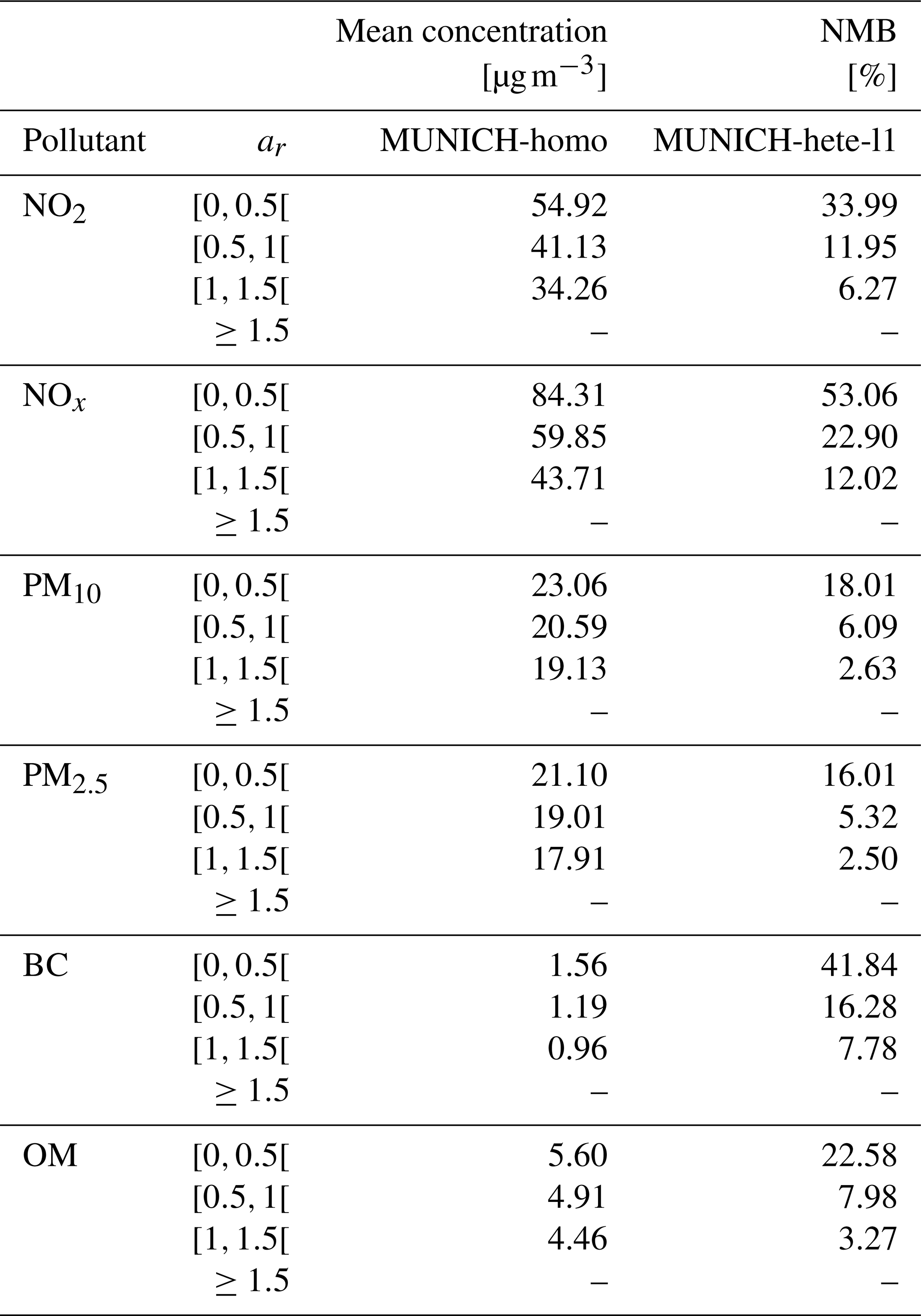
Table 1 and Appendix F present the influence of the aspect ratio on concentrations in the first vertical level of the heterogeneous version of MUNICH, MUNICH-hete-l1, compared to the homogeneous version. It is quantified using the normalized mean bias (NMB). The homogeneous version of MUNICH presents higher concentrations of pollutants in wide streets (interval [0,0.5[) in greater Paris due to higher traffic emissions compared to in narrower streets. The increase in the concentration in the first level as a result of using the heterogeneous version of the model is more important for wide streets (up to 53 % for NO_x). Concerning particles, PM₁₀ concentrations are increased by up to 18 %, while the increase is about 42 % and 23 % for BC and OM respectively. In streets with larger a_r (interval [1,1.5[), NO_x concentrations are only 12 % higher than in the homogeneous version, and the PM₁₀ concentrations are only 2.5 % higher.

Concerning the two cases in Copenhagen, CO and NO_x concentrations present similar behaviour in comparison to the greater Paris case. For the JGTV street network, the increase is limited compared to the HCAB network – 3 % against 11.5 % respectively for CO. Wide streets (interval [0,0.5[) have higher concentrations of NO₂ compared to the homogenous version of MUNICH, whereas for the other intervals of a_r, they are lower. Thus, O₃ concentrations are lower for wide streets and larger for the other intervals. This could be linked to the lack of volatile organic compounds in these two Copenhagen cases.

Table 1 Statistical indicators of the influence of the aspect ratio on concentrations in MUNICH-hete-l1 for the street network in greater Paris. Indicators are presented in Appendix B.

5.2 Sensitivity to the street network

The computation of inflow and outflow fluxes at intersections is performed by estimating the balance of fluxes entering and leaving the intersection from the different street segments attached to it. If this balance is not perfect, there are exchanges with the atmosphere above the intersection. When the total flux entering the intersection is higher than the one leaving it, the flow overload is directed to the atmosphere. When the total flux leaving the intersection is higher, a flux from the atmosphere to the intersection is considered. A further explanation is available in Kim et al. (2018, 2022).

Without a street network around the street segment of interest, the pollutant mass fluxes entering the street are determined from the background concentration. The contribution of the neighbouring streets is thus not taken into account, and concentrations of pollutants emitted in streets are expected to be lower than when there is a street network.

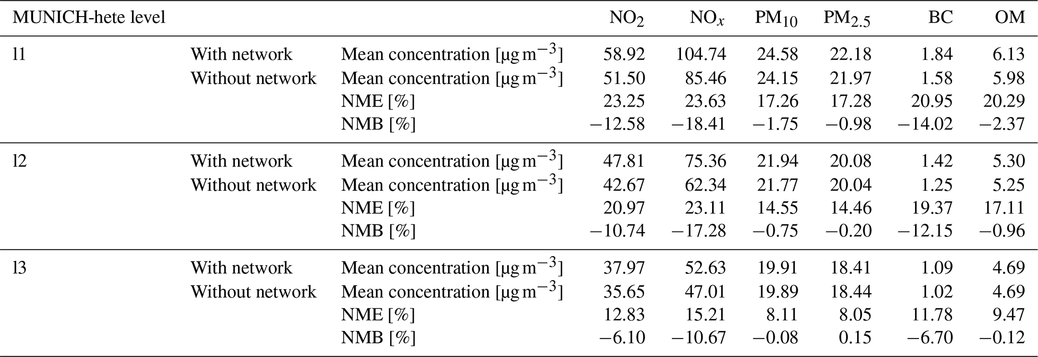
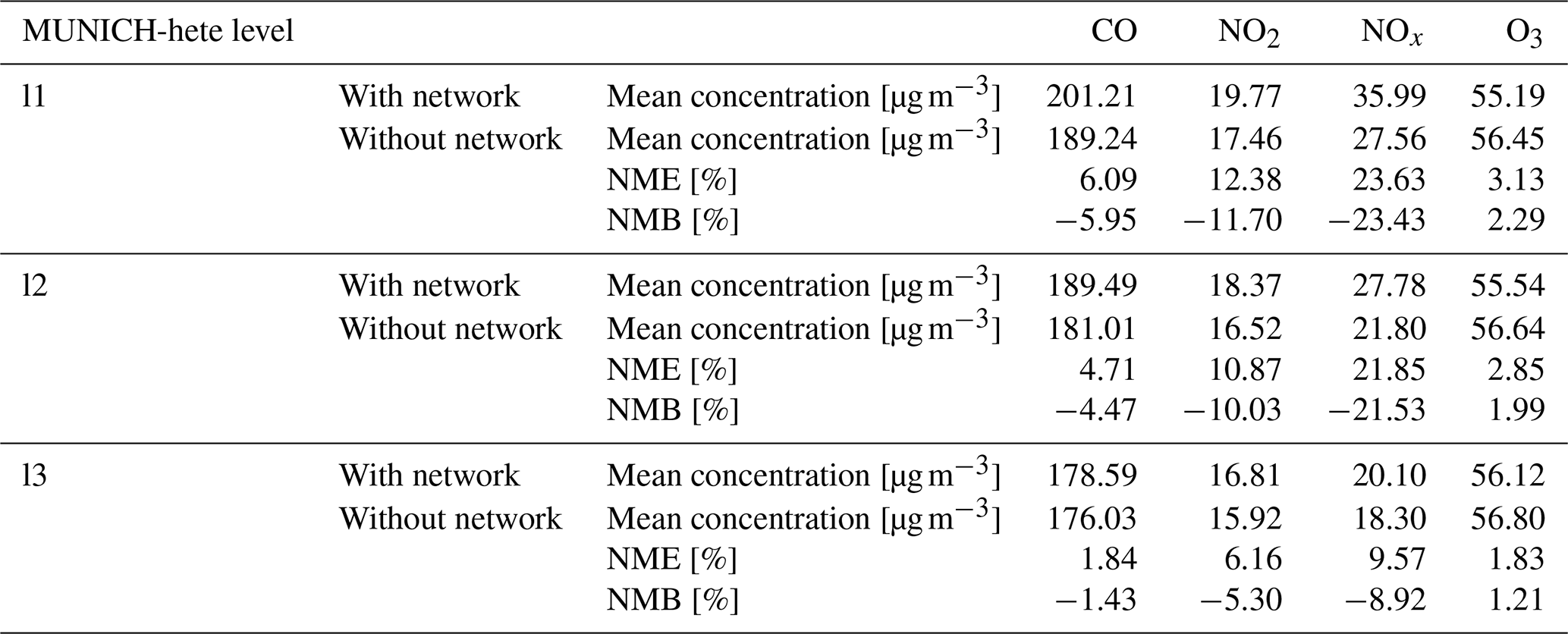
Table 2 and Appendix G present the influence of the neighbouring streets for the three cases of the study. It is quantified using the normalized mean error (NME) and NMB between the simulations without and with the neighbouring streets. As expected, without the street network, the concentrations are lower. The bias is between 12 % and 21 % for NO₂, between 18 % and 27 % for NO_x, and 14 % for BC. Biases are lower for OM and PM (2 %) because of the stronger influence of background concentrations for those compounds.

Table 2 Statistical indicators of the influence of the street network on concentrations simulated with MUNICH-hete for the street segment of the Boulevard d'Alsace Lorraine with the monitoring station. Indicators are presented in Appendix B.

6 Conclusions

The street-network model MUNICH v2.0 has been modified to introduce concentration heterogeneities in the street and to better represent population exposure. To model the vertical gradients frequently observed, the streets were discretized with three levels, thus limiting the artificial dilution of emissions and concentrations. Based on a parameterization from OSPM, a ventilation zone is considered under specific conditions to represent horizontal heterogeneities. In order to test these developments, the heterogeneous version of MUNICH (MUNICH-hete) has been applied to two cases in Copenhagen, Denmark, with comparisons to OSPM, and to one case near Paris, France. Overall, MUNICH-hete improves the comparison to observations compared to the homogeneous version. The errors compared to observations are reduced by up to 20 % for NO_x and up to 15 % for BC.

As expected, in MUNICH-hete, concentrations of compounds emitted by traffic (CO, NO₂, NO_x, PM₁₀, BC, and OM) are higher at the bottom of the street than at the top. These increases can reach up to 60 % and 30 % for NO₂ and PM₁₀ respectively. The intermediate level, serving as a buffer, presents concentrations higher than or similar to the homogeneous version (MUNICH-homo). Finally, concentrations in the highest level, in direct contact with the atmosphere above the street, are the lowest of the street. For the Danish cases, the low NO₂ concentrations observed in the lower levels could be related to the absence of volatile organic compounds in the model setup and the coarse vertical discretization limiting O₃ transport deep into the street.

A sensitivity study of the influence of the street network on concentrations in the streets shows the importance of considering neighbouring streets in MUNICH. When no network is considered, concentrations in the street are lower due to the overestimated impact of the atmosphere above. At the bottom of the street, concentrations of NO₂ and BC are reduced by up to 28 % and 14 % respectively without a network. PM and OM are less impacted, with a reduction of about 2 % due to a strong influence of non-traffic sources.

For the next step, the ventilation zone will be fully discretized vertically to facilitate the penetration of background concentrations into the bottom of the street. The horizontal exchange fluxes between the two zones will also be modelled. Deposition and resuspension processes that were not considered in this development will be added. The fluxes that are currently assumed to be vertically homogeneous will be discretized. Finally, chemistry of volatile organic compounds could be added in the Danish cases if the background concentrations and emissions are available.

Appendix A: Volumes of the recirculation and ventilation zones

The algorithm used in the heterogeneous version of MUNICH to compute the volumes of the recirculation and ventilation zones is based on the parameterization of OSPM (Berkowicz et al., 1997; Berkowicz, 2000b; Ottosen et al., 2015). This algorithm is applied at the beginning of each time step as the size of the recirculation zone is dependent on wind speed and direction. Figure A1 presents the shape of the recirculation zone and the associated parameters.

Figure A1 Representation of the recirculation zone in the heterogeneous version of MUNICH.

The first step is to compute the length of the vortex in the direction of the wind:

$$\begin{array}{}\text{(A1)}& L_{\text{vortex}}=\mathrm{2}Hf,\end{array}$$

with H being the height of the street, and

$$\begin{array}{}\text{(A2)}& {\displaystyle }f=\left\{\begin{array}{ll}\mathrm{1}& \text{if }{u}_{\text{roof}}\ge \mathrm{2}\mathrm{m}{\mathrm{s}}^{-\mathrm{1}}\\ \sqrt{\mathrm{0.5}{u}_{\text{roof}}}& \text{if }{u}_{\text{roof}}<\mathrm{2}\mathrm{m}{\mathrm{s}}^{-\mathrm{1}},\end{array}\right.\end{array}$$

with u_roof being the wind speed at roof level.

The width of the trapeze base is the projection of L_vortex in the street:

$$\begin{array}{}\text{(A3)}& W_{\text{base}}=L_{\text{vortex}}\sin \left(\mathit{\theta }\right),\end{array}$$

with θ being the angle between the wind direction and the street orientation.

The width of the trapeze top is equal to half of the base:

$$\begin{array}{}\text{(A4)}& W_{\mathrm{3}}={\displaystyle \frac{L_{\text{vortex}}\sin \left(\mathit{\theta }\right)}{\mathrm{2}}}.\end{array}$$

Knowing these lengths and using algebraic considerations, the widths W₁ and W₂ can be calculated:

$$\begin{array}{}\text{(A5)}& \left\{\begin{array}{l}{W}_{\mathrm{1}}=W_{\mathrm{3}}+{\displaystyle \frac{(h_{\mathrm{2}}+h_{\mathrm{3}})\mathrm{\Delta }W}{H}}\\ W_{\mathrm{2}}=W_{\mathrm{3}}+{\displaystyle \frac{h_{\mathrm{3}}\mathrm{\Delta }W}{H}}\end{array}\right.,\end{array}$$

with $\mathrm{\Delta }W=W_{\text{base}}-W_{\mathrm{3}}$.

The horizontal surfaces for vertical exchanges between the levels and with the concentrations above the street are calculated as follows:

$$\begin{array}{}\text{(A6)}& \left\{\begin{array}{l}{S}_{\mathrm{1}}^{\mathrm{h}}=W_{\mathrm{1}}L\\ S_{\mathrm{2}}^{\mathrm{h}}=W_{\mathrm{2}}L\\ S_{\mathrm{3}}^{\mathrm{h}}=W_{\mathrm{3}}L\end{array}\right.,\end{array}$$

with L being the street length.

The vertical surfaces for advection via intersections are determined with the following:

$$\begin{array}{}\text{(A7)}& \left\{\begin{array}{l}{S}_{\mathrm{1}}^{\mathrm{v}}={\displaystyle \frac{W_{\mathrm{1}}\left(h_{\mathrm{1}}{)}^{\mathrm{2}}\right(W_{\text{base}}-W_{\mathrm{1}})}{\mathrm{2}}}\\ S_{\mathrm{2}}^{\mathrm{v}}={\displaystyle \frac{W_{\mathrm{2}}\left(h_{\mathrm{2}}{)}^{\mathrm{2}}\right(W_{\mathrm{1}}-W_{\mathrm{2}})}{\mathrm{2}}}\\ S_{\mathrm{3}}^{\mathrm{v}}={\displaystyle \frac{W_{\mathrm{3}}\left(h_{\mathrm{3}}{)}^{\mathrm{2}}\right(W_{\mathrm{2}}-W_{\mathrm{3}})}{\mathrm{2}}}\end{array}\right..\end{array}$$

Finally, the volumes associated with each level of the recirculation zone are

$$\begin{array}{}\text{(A8)}& \left\{\begin{array}{l}{V}_{\mathrm{1}}=h_{\mathrm{1}}L\left(W_{\mathrm{1}}+{\displaystyle \frac{(W_{\text{base}}-W_{\mathrm{1}})}{\mathrm{2}}}\right)\\ V_{\mathrm{2}}=h_{\mathrm{2}}L\left(W_{\mathrm{2}}+{\displaystyle \frac{(W_{\mathrm{1}}-W_{\mathrm{2}})}{\mathrm{2}}}\right)\\ V_{\mathrm{3}}=h_{\mathrm{3}}L\left(W_{\mathrm{3}}+{\displaystyle \frac{(W_{\mathrm{2}}-W_{\mathrm{3}})}{\mathrm{2}}}\right)\end{array}\right..\end{array}$$

In the current version of MUNICH-hete, it is assumed that traffic emissions are all affected to the recirculation zone. Therefore, its base W_base has to be superior or equal to the street width W. If this is not the case, the recirculation zone is considered to fill the whole street volume.

When considered, the other widths are also limited by the street width:

$$\begin{array}{}\text{(A9)}& \left\{\begin{array}{l}{W}_{\mathrm{1}}=min(W,W_{\mathrm{1}})\\ W_{\mathrm{2}}=min(W,W_{\mathrm{2}})\\ W_{\mathrm{3}}=min(W,W_{\mathrm{3}})\end{array}\right..\end{array}$$

Appendix B: Statistical indicators

For evaluation of the simulations compared to observations, the following statistical indicators are used. o and s represent the observed and the simulated concentrations respectively. The overbar represents the average.

• Mean fractional error (MFE):

  $$\text{MFE}=\mathrm{2}\times \stackrel{\mathrm{‾}}{\left({\displaystyle \frac{|s-o|}{s+o}}\right)}.$$

• Mean fractional bias (MFB):

  $$\text{MFB}=\mathrm{2}\times \stackrel{\mathrm{‾}}{\left({\displaystyle \frac{s-o}{s+o}}\right)}.$$

• Factor of 2 (FAC2): fraction of data that satisfy $\mathrm{0.5}\le \frac{s}{o}\le \mathrm{2.0}$.

For comparison of the simulations, the normalized mean bias (NMB) and normalized mean error (NME) are used. X represents concentrations, with X₀ being the reference simulation and X_i being the compared simulation. The overbar represents the average.

• Normalized mean bias:

  $$\text{NMB}={\displaystyle \frac{\stackrel{\mathrm{‾}}{(X_i-X_{\mathrm{0}})}}{\stackrel{\mathrm{‾}}{X_{\mathrm{0}}}}}.$$

• Normalized mean error:

  $$\text{NME}={\displaystyle \frac{\stackrel{\mathrm{‾}}{\left|X_i-X_{\mathrm{0}}\right|}}{\stackrel{\mathrm{‾}}{X_{\mathrm{0}}}}}.$$

Appendix C: Additional information for HCAB

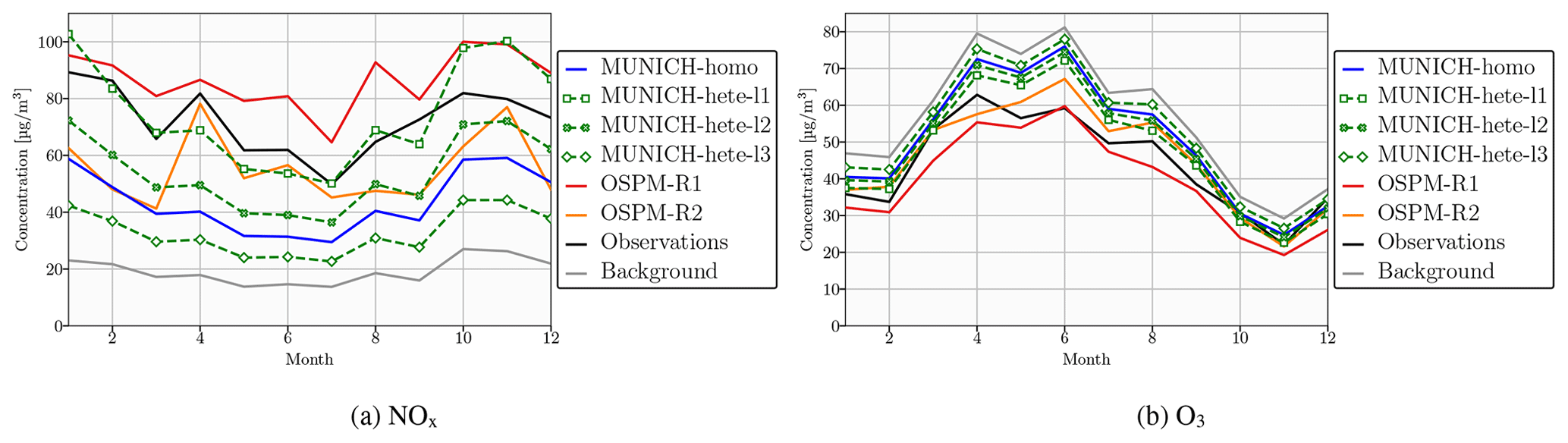
Figure C1 Monthly averaged concentrations (in µg m⁻³) of NO_x (a) and O₃ (b) at HCAB monitoring station. The solid blue line represents the homogeneous version of MUNICH. The three dashed green lines represent the three levels of the heterogeneous version of MUNICH – the lowest level (l1) is shown with square markers, the intermediate level (l2) is shown with crossed markers, and the top level (l3) is shown with diamond markers. The solid red line represents the OSPM receptor that is close to the measurement station, and the solid orange line represents the second OSPM receptor located on the other side of the street. The observations are in solid black, and the background concentrations are in solid grey.

Table C1 Statistical indicators of the evaluation of the hourly simulated concentrations compared to observations at HCAB monitoring station. Indicators are presented in Appendix B.

Appendix D: Additional information for JGTV

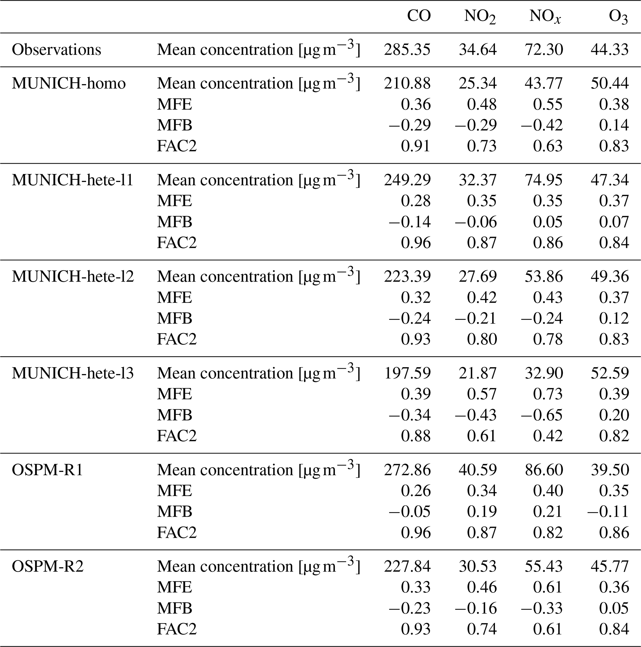
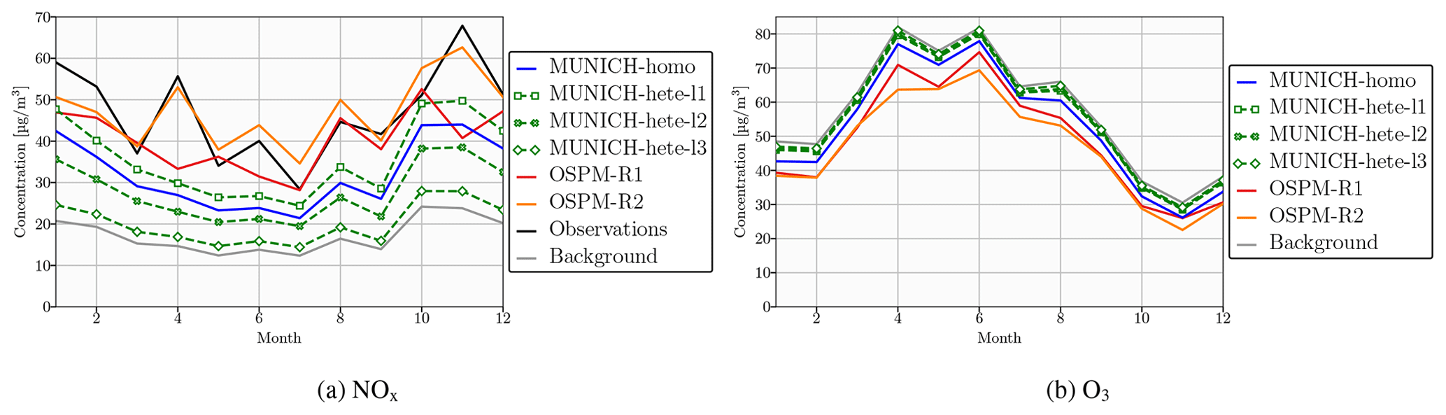
Figure D1 Monthly averaged concentrations (in µg m⁻³) of NO_x (a) and O₃ (b) at JGTV monitoring station. The solid blue line represents the homogeneous version of MUNICH. The three dashed green lines represent the three levels of the heterogeneous version of MUNICH – the lowest level (l1) is shown with square markers, the intermediate level (l2) is shown with crossed markers, and the top level (l3) s shown with diamond markers. The solid orange line represents the OSPM receptor that is close to the measurement station, and the solid red line represents the second OSPM receptor located on the other side of the street. The observations are in solid black, and the background concentrations are in solid grey.

Table D1 Statistical indicators of the evaluation of the hourly simulated concentrations compared to observations at JGTV monitoring station. Indicators are presented in Appendix B.

Appendix E: Additional information for the district of Le Perreux-sur-Marne

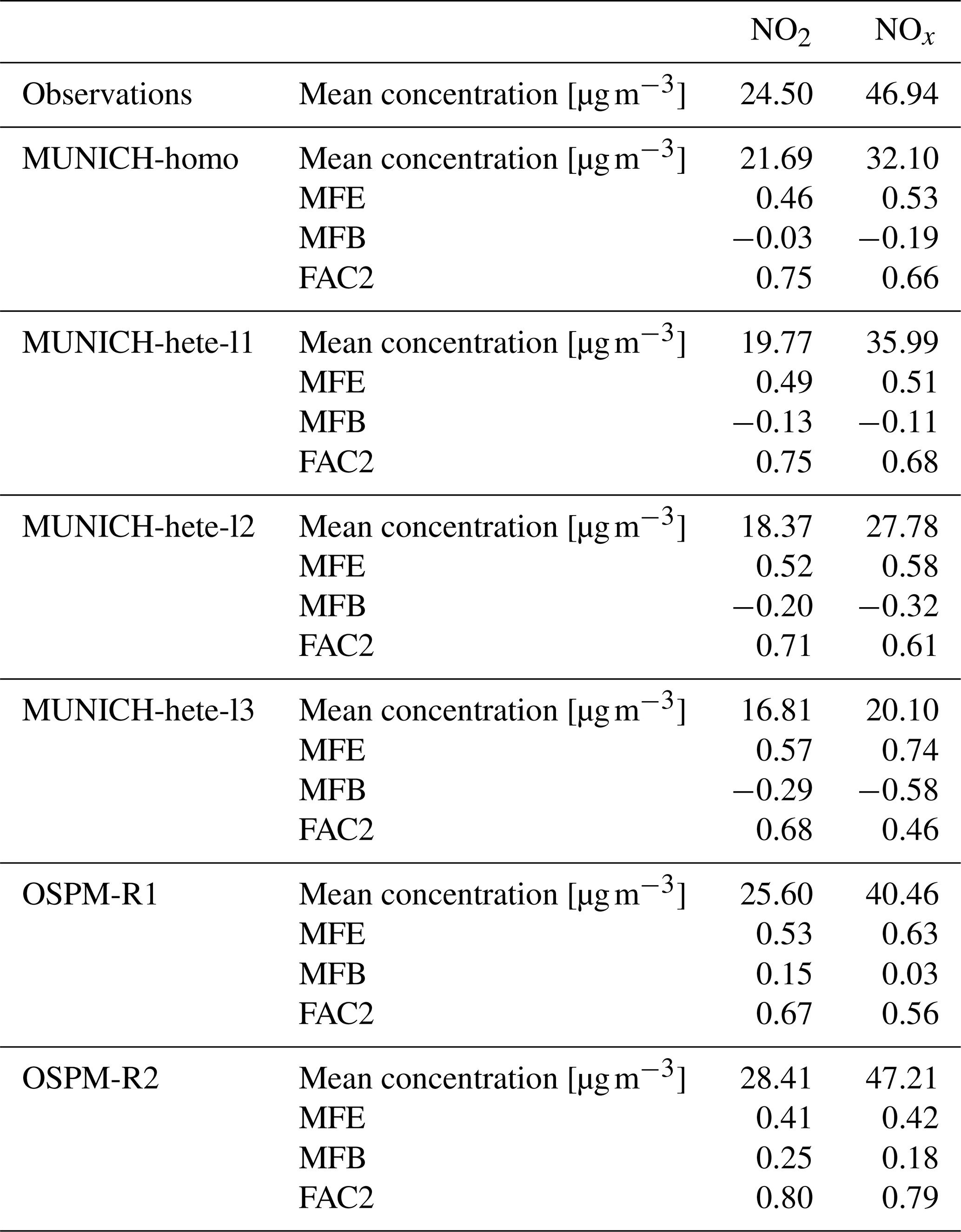
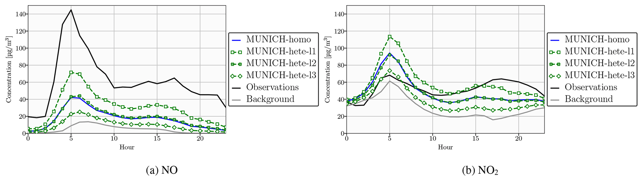
Figure E1 Average daily profile of the concentrations of NO (a) and NO₂ (b) over the simulation period at the Boulevard d'Alsace Lorraine monitoring station. The solid blue line represents the homogeneous version of MUNICH. The three dashed green lines represent the three levels of the heterogeneous version of MUNICH – the lowest level (l1) is shown with square markers, the intermediate level (l2) is shown with crossed markers, and the top level (l3) is shown with diamond markers. The observations are in solid black, and the background concentrations are in solid grey.

Table E1 Statistical indicators of the evaluation of the hourly simulated concentrations to observations at the Boulevard d'Alsace Lorraine monitoring station. Indicators are presented in Appendix B.

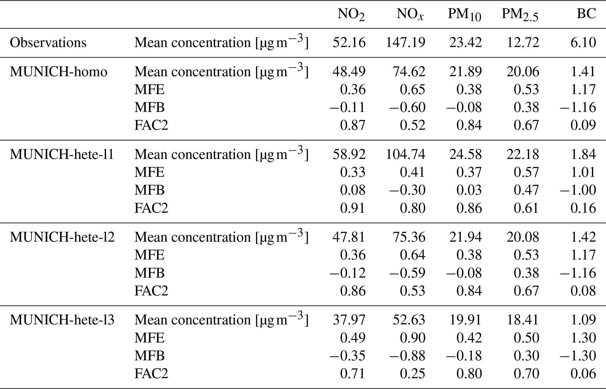
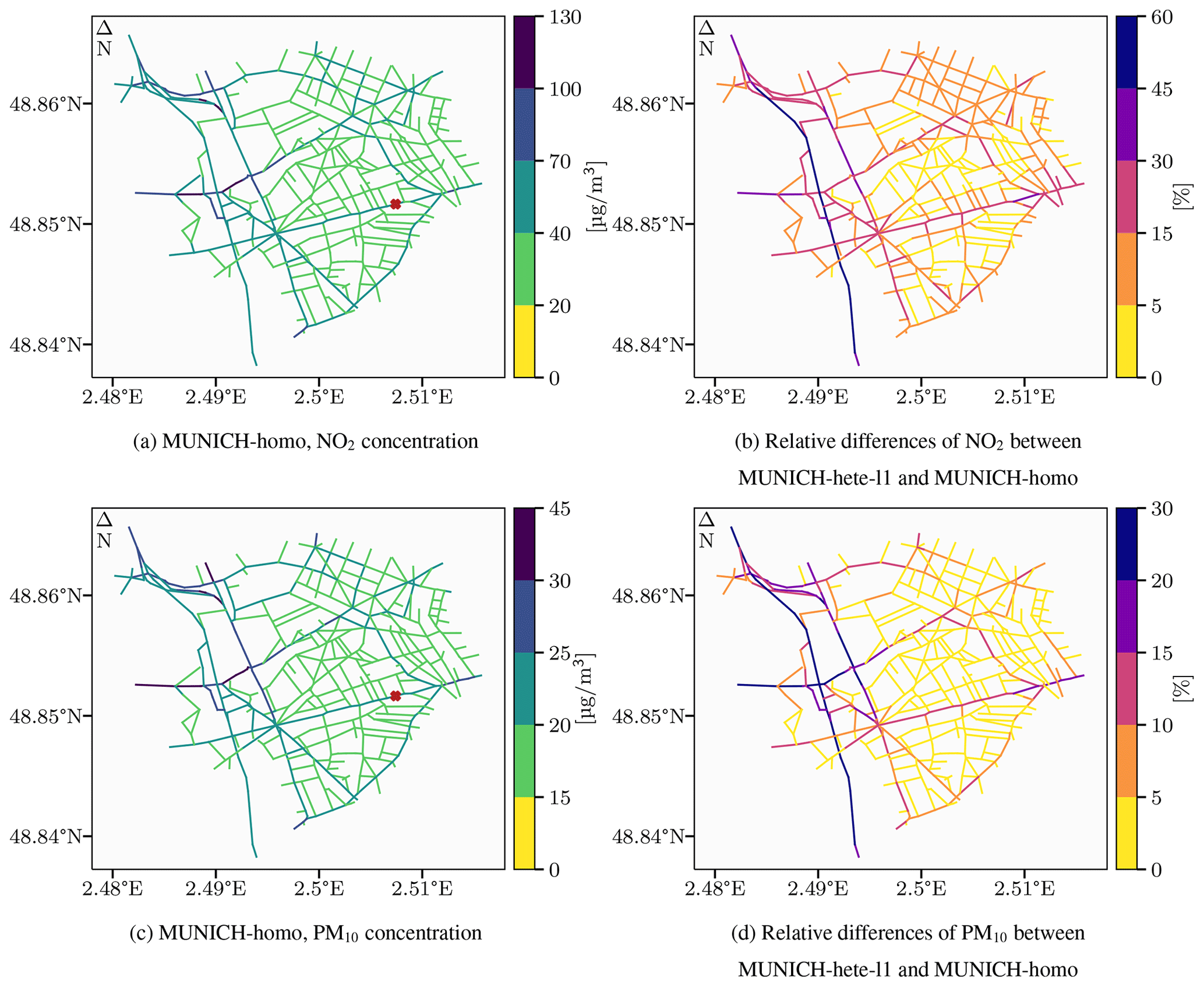
Figure E2 NO₂ and PM₁₀ time-averaged concentrations (in µg m⁻³) for MUNICH-homo in the left panel (a, c) for the district of Le Perreux-sur-Marne. Relative differences (in %) between the first level of MUNICH-hete and MUNICH-homo for NO₂ and PM₁₀ in the right panel (b, d) for the district of Le Perreux-sur-Marne. A positive relative difference indicates higher concentrations for MUNICH-hete. The brown cross in panels (a) and (c) represents the position of the measurement station.

Appendix F: Additional information for the influence of the aspect ratio

Table F1 Statistical indicators of the influence of the aspect ratio on concentrations in MUNICH-hete-l1 for the street network around HCAB. Indicators are presented in Appendix B.

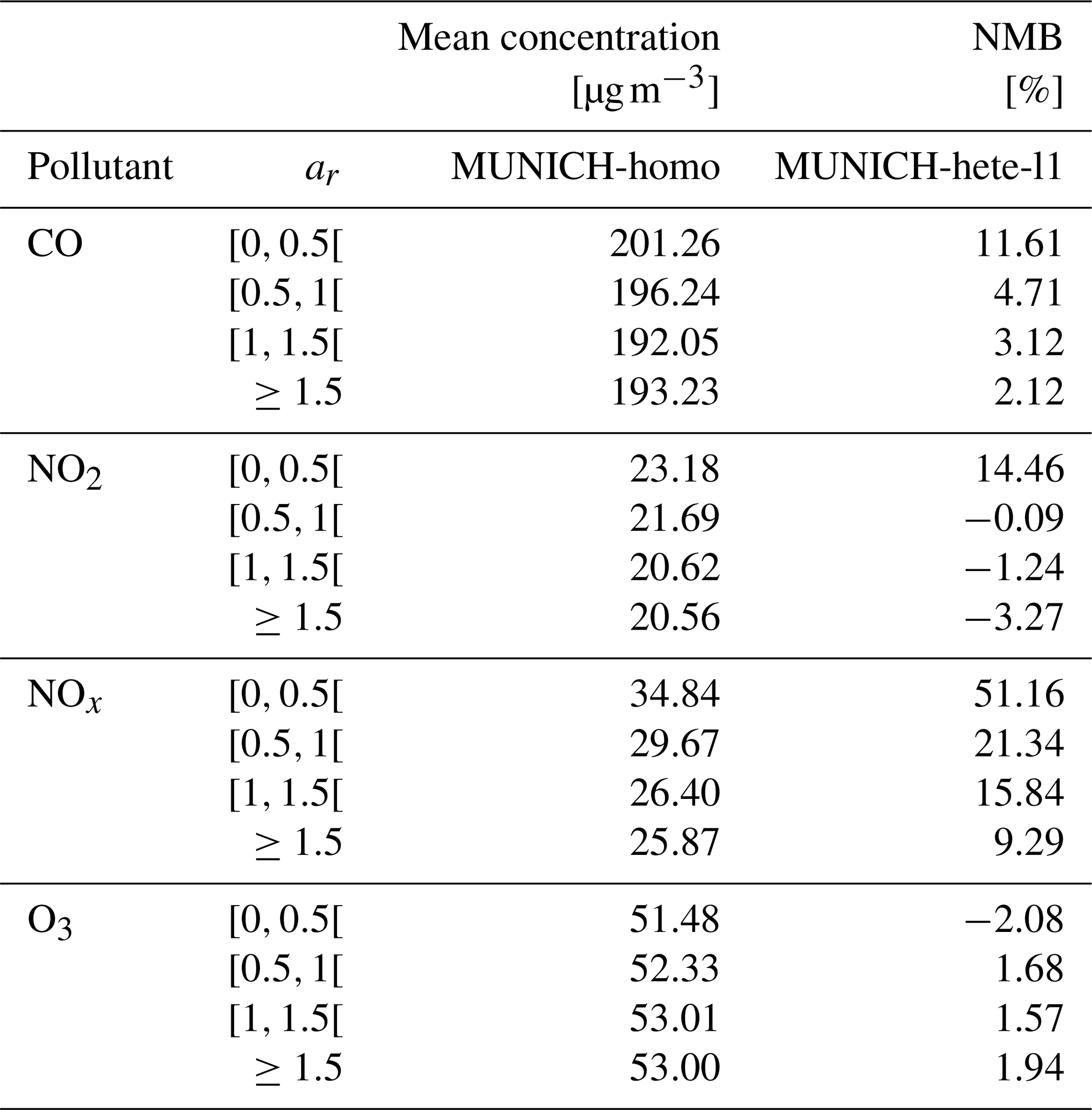
Table F2 Statistical indicators of the influence of the aspect ratio on concentrations in MUNICH-hete-l1 for the street network around JGTV. Indicators are presented in Appendix B.

Appendix G: Additional information for the sensitivity to street network

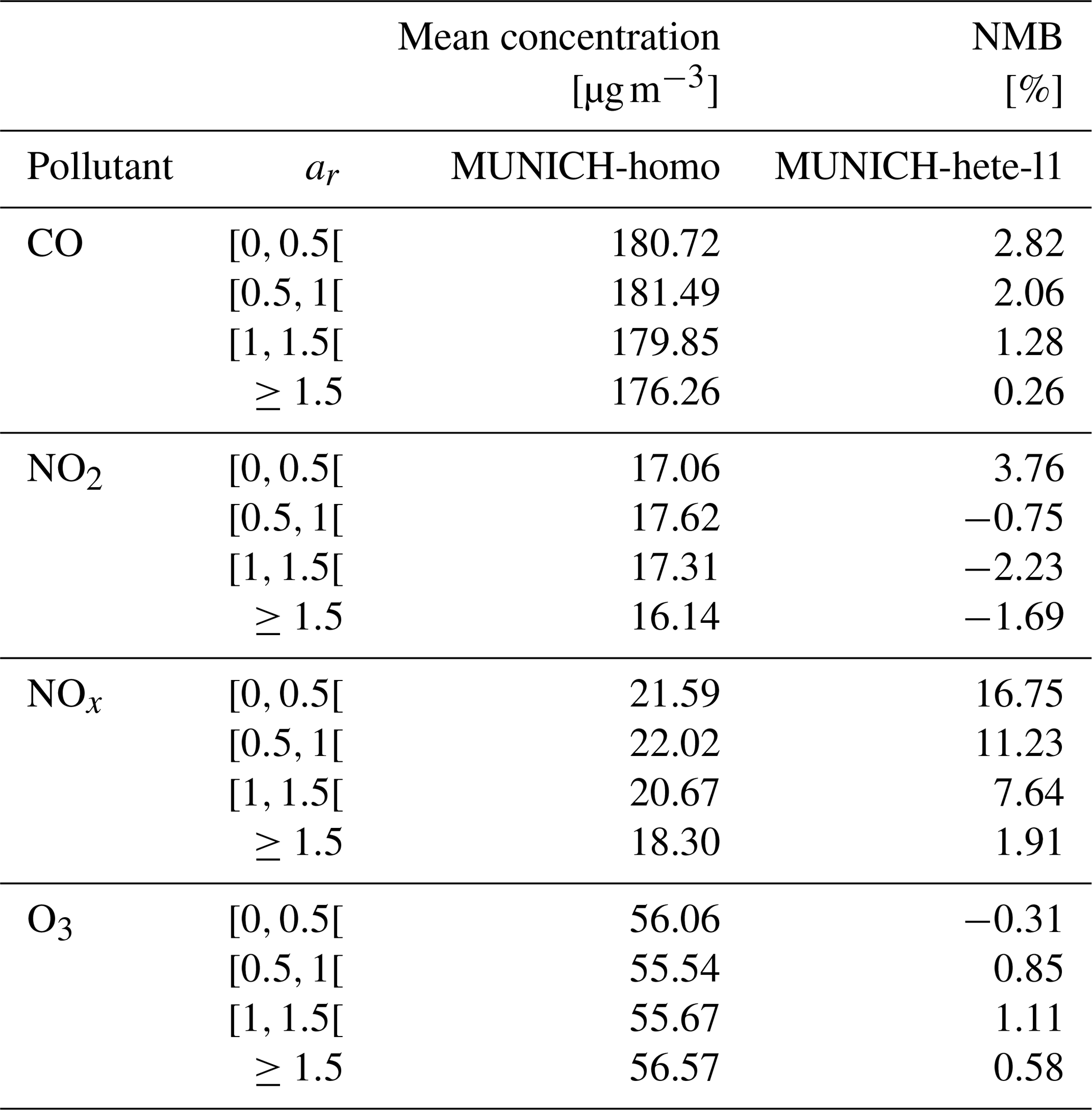
Table G1 Statistical indicators of the influence of the street network on concentrations simulated with MUNICH-hete for the street segment HCAB with the monitoring station. Indicators are presented in Appendix B.

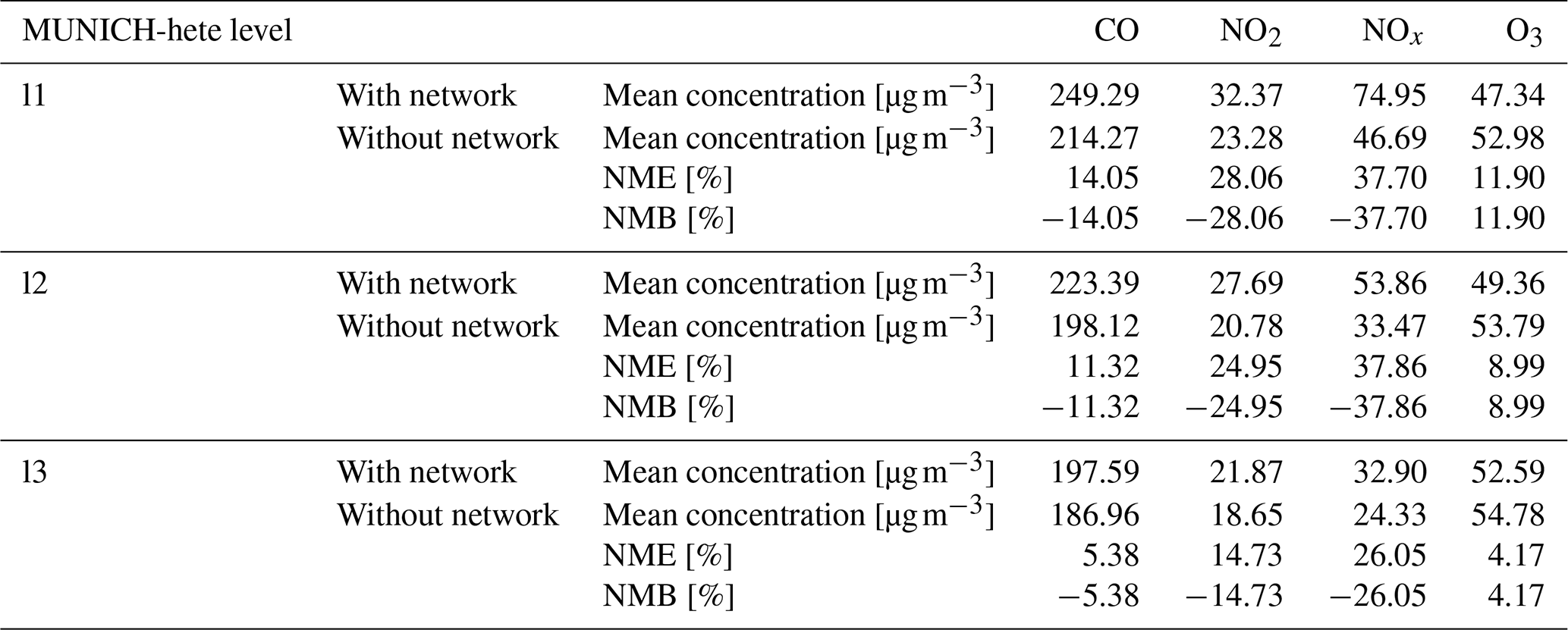
Table G2 Statistical indicators of the influence of the street network on concentrations simulated with MUNICH-hete for the street segment JGTV with the monitoring station. Indicators are presented in Appendix B.