Metrics for evaluating the quality in linear atmospheric inverse problems: a case study of a trace gas inversion

Several metrics have been proposed and utilized to diagnose the performance of linear Bayesian and geostatistical atmospheric inverse problems. These metrics primarily assess the reductions in the prior uncertainties, compare modeled observations to true observations, and check distributional assumptions. Although important, these metrics should be augmented with a sensitivity analysis to obtain a comprehensive understanding of the atmospheric inversion performance and improve the quality and confidence in the inverse estimates. In this study, we derive closed-form expressions of local sensitivities for various input parameters, including measurements, covariance parameters, covariates, and a forward operator. To further enhance our understanding, we complement the local sensitivity analysis with a framework for a global sensitivity analysis that can apportion the uncertainty in input parameters to the uncertainty associated with inverse estimates. Additionally, we propose a mathematical framework to construct nonstationary correlation matrices from a precomputed forward operator, which is closely tied to the overall quality of inverse estimates. We demonstrate the application of our methodology in the context of an atmospheric inverse problem for estimating methane fluxes in Los Angeles, California.

1 Introduction

In atmospheric applications, inverse models are frequently used to estimate global- to regional-scale fluxes of trace gases from atmospheric measurements (Enting, 2002). At a global scale, data assimilation remains the primary inverse modeling framework, which assimilates observations sequentially and updates the prior estimates of fluxes by utilizing an atmospheric model coupled with chemistry (for further details on data assimilation, see Wikle and Berliner, 2007). At a regional scale, inversions that assimilate all observations simultaneously by utilizing a precomputed forward operator (Lin et al., 2003) that describes the relationship between observations and fluxes are commonly used (for details, see Enting, 2002). This work focuses on the use of precomputed forward operators for atmospheric inverse modeling and addresses the sensitivity analysis and correlation in the forward operator in the context of Bayesian (e.g., Lauvaux et al., 2016) and geostatistical inverse methods (e.g., Kitanidis, 1996).

The sensitivity analysis in this work is covered under local and global themes. Primarily, we focus on local sensitivity analysis (LSA), which measures the effect of a given input on a given output and is obtained by computing the partial derivatives of an output quantity of interest for an input factor (see Rabitz, 1989, and Turányi, 1990). Within the global theme (designated as a global sensitivity analysis), we focus on how uncertainty in the model output can be apportioned to different model input parameters (Saltelli et al., 2008).

Overall, in atmospheric trace gas inversions, the LSA is mostly performed. Within this context, the LSA assesses how sensitive the posterior estimates of fluxes are regarding the underlying choices or assumptions, like the (1) observations included, (2) model data error covariance, (3) input prior information and its error, and (4) forward operator (for a discussion, see Michalak et al., 2017). This task is sometimes performed to arrive at a robust estimate of fluxes and their uncertainties by running an inverse model multiple times, while varying the input parameters and assessing their impact on the estimated fluxes and uncertainties. Another complementary way to do the LSA is by computing the local partial derivatives of input parameters that go into an inversion.

The LSA can be grouped with standard information content approaches such as an averaging kernel and degrees of freedom for signal (DOFS; for details, see Sect. 2.2.1 of this paper, Rodgers, 2000, and Brasseur and Jacob, 2017). However, the LSA is more informative than these approaches alone, as it examines individual components (see Sect. 2.2) that determine DOFS and quantifies the impact and relative importance of various components of an inversion.

In this study, we focus on the quality of the inverse estimates of the fluxes, which means providing diagnostic metrics to improve our understanding of the impact of input choices on the inverse estimates of fluxes and thus improve the quality of the inverse model. Specifically, in this technical note, we provide (1) closed-form expressions to conduct LSA by computing partial derivatives, (2) a scientifically interpretable framework for ranking thousands of spatiotemporally correlated input parameters with the same or different units of measurement, (3) a mathematical schema for conducting a global sensitivity analysis (GSA), and (4) a technique to assess the spatiotemporal correlation between the forward operators of two or multiple observations, which is tied to the overall diagnostics of the estimated fluxes and can lead to improved representation of errors in the forward operator.

2 Methods and derivation

In generic form, a linear inverse problem can be written as follows:

$$\begin{array}{}\text{(1)}& \mathit{z}=\mathbf{H}\mathit{s}+\mathit{ϵ},\end{array}$$

where H is a forward operator that maps model parameters (fluxes in the context of this work) to measurements z and encapsulates our understanding of the physics of the measurements. The error ϵ in Eq. (1) describes the mismatch between measurements and the modeled measurements (see Sect. 3).

In a typical linear atmospheric inverse problem (see Fig. 1), the estimates of fluxes (box 8 in Fig. 1) are obtained in a classical one-stage-batch Bayesian setup (for details, see Enting, 2002; Tarantola, 2005). In this setup, the a priori term (box 3 in Fig. 1) is based on a fixed flux pattern, and the errors (box 6 in Fig. 1) are either assumed to be independent or are governed by a predefined covariance structure (for details, see Gurney et al., 2003; Rödenbeck et al., 2003, 2006).

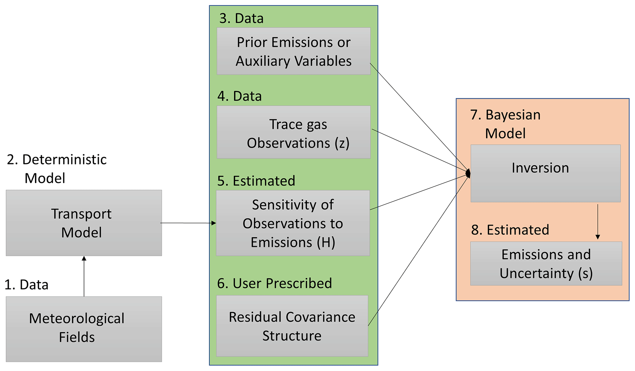
Figure 1 The schema for performing a linear atmospheric inversion to obtain the estimates of the emissions of greenhouse gases. The middle column (the box with a green background) lists all of the input parameters that are required to perform an inversion, whereas the right column (the box with an orange background) lists the modeling process (box 7) and the output obtained after performing an inversion (box 8). Note that this work focuses on understanding and ranking the impact of the input parameters (boxes 3, 4, and 6) on the estimates of fluxes (box 8) and developing correlation structures from the forward operator (box 5).

Within the previously mentioned setup, the choice of the input parameters, including the forms of error structures, profoundly impacts the quality of the inverse estimates of fluxes. Understanding the impact of these input parameters is critical for evaluating the quality of the estimated fluxes. Thus, we first (Sect. 2.1) utilize the understanding of the physics of the measurements, encapsulated in H, to generate scientifically interpretable correlation matrices (box 6 in Fig. 1). Second, we assess and rank the importance of the input parameters (Sect. 2.2) shown in the middle column (the box with a green background ) in Fig. 1 (box 8 in Fig. 1), which is finally followed by a methane (CH₄) case study that demonstrates the applicability of our methods (see Sect. 2).

2.1 Analysis of the forward operator

In inversions that assimilate all observations simultaneously, a forward operator for each observation included in an inversion is obtained from a transport model. These observations can be obtained from multiple platforms, including an in situ network of fixed locations on the surface, intermittent aircraft flights, and satellites. In most situations, the spatiotemporal coverage of these forward operators is visually assessed by plotting an aggregated sum or mean of their values over a spatial domain. However, the standard quantitative metrics to evaluate their coverage and intensity in space and time remain absent. In this study, we present two metrics for this assessment, which are defined below. These metrics are in accordance with the triangular inequality and are distances in their respective metric spaces.

Note that, in the published literature on trace gas inversions, sometimes the forward operator obtained from a transport model is referred to as a sensitivity matrix, Jacobian, or footprint. Henceforth, we always refer to the Jacobian, sensitivity matrix, or footprint as a forward operator to avoid misinterpretation. We show our application through forward operators constructed by running a Lagrangian transport model. However, the proposed methods can also be applied in the Eulerian framework (see Brasseur and Jacob, 2017, for details).

2.1.1 Integrated area overlap measurement index (IAOMI)

The integrated area overlap measurement index (IAOMI) summarizes the shared information content between two forward operators and hence indirectly between two observations. It is, therefore, a measure of the uniqueness of the flux signal associated with an observation compared to other observations.

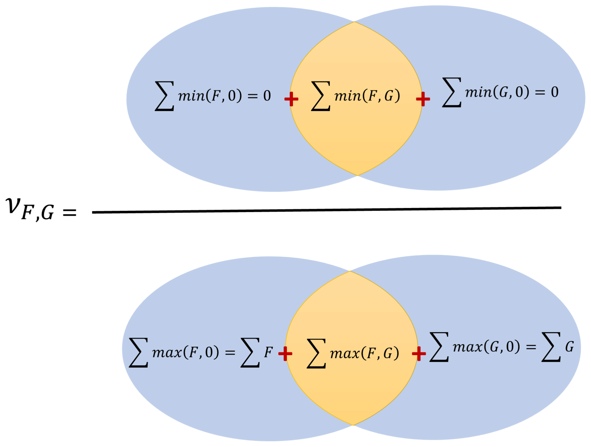
Figure 2 A Venn diagram that defines IAOMI in terms of two hypothetical forward operators F and G.

Intuitively, IAOMI can be better understood spatially. For a given time point, consider two forward operators F and G as the two vector-valued functions over an area. The IAOMI index is the proportion of the common contribution of the two forward operators for the intersected area with respect to the overall contribution of the two forward operators. This is demonstrated through a Venn diagram in Fig. 2. Thus, IAOMI can be defined as follows:

$$\begin{array}{}\text{(2)}& {\mathit{\nu }}_{\mathbf{F},\mathbf{G}}={\displaystyle \frac{{\mathrm{\Sigma }}_{A_{\mathbf{F}}\cap A_{\mathbf{G}}}{\mathbf{f}}_{\mathrm{1}}(\mathbf{F},\mathbf{G})}{{\mathrm{\Sigma }}_{A_{\mathbf{F}}\cup A_{\mathbf{G}}}{\mathbf{f}}_{\mathrm{2}}(\mathbf{F},\mathbf{G})}},\end{array}$$

where, for any forward operator S, the corresponding set A_S, on which the forward operator is always positive, is defined as $A_{\mathbf{S}}=\mathit{\{}\mathit{x}:\mathbf{S}(\mathit{x})>\mathrm{0}\mathit{\}}$ and the two vector-valued functionals f₁ and f₂ can be given as follows:

$$\begin{array}{}\text{(3)}& \begin{array}{rl}& {\mathbf{f}}_{\mathrm{1}}(\mathbf{F},\mathbf{G})=\left\{\begin{array}{ll}min(\mathbf{F},\mathbf{G})& \text{on}{A}_{\mathbf{F}}\cap A_{\mathbf{G}}\\ \mathrm{0}& \text{otherwise}\end{array}\right.\\ & \text{and}\\ & {\mathbf{f}}_{\mathrm{2}}(\mathbf{F},\mathbf{G})=\left\{\begin{array}{ll}max(\mathbf{F},\mathbf{G})& \text{on}{A}_{\mathbf{F}}\cap A_{\mathbf{G}}\\ \mathbf{F}& \text{on}{A}_{\mathbf{F}}\cap A_{\mathbf{G}}^c\\ \mathbf{G}& \text{on}{A}_{\mathbf{F}}^c\cap A_{\mathbf{G}}\end{array}\right.\end{array}.\end{array}$$

Note that the IAOMI defined in Eq. (2) can also be written as a ratio of the sum of minimums over the sum of the maximums, as follows:

$$\begin{array}{}\text{(4)}& {\mathit{\nu }}_{\mathbf{F},\mathbf{G}}={\displaystyle \frac{{\mathrm{\Sigma }}_{A_{\mathbf{F}}\cup A_{\mathbf{G}}}min(\mathbf{F},\mathbf{G})}{{\mathrm{\Sigma }}_{A_{\mathbf{F}}\cup A_{\mathbf{G}}}max(\mathbf{F},\mathbf{G})}}.\end{array}$$

IAOMI ν can also be thought of as a measure of the similarity between two forward operators. It is evident from Eq. (4) that this is a weighted Jaccard similarity index or Ruzicka index (Cha, 2007), which describes the similarity between two forward operators F and G. It follows that ν is closed and bounded in [0,1] and accounts for both the spatiotemporal spread and the intensity of the forward operator. A stronger ν implies that there is a larger overlap of the intensity in space and time, that it is analogous to finding the common area within two curves, and that it is indicative of the magnitude of overlapping information, knowledge which is beneficial in the context of satellite observations with a higher potential for sharing information content.

A dissimilarity measure can be obtained from ν and be defined by 1−ν. The smaller the overlap or the larger the value of 1−ν, the more significant the disparity. Note that the ν metric is only indicative of the overlap in the spatiotemporal intensity between two forward operators. To measure how much of the shared intensity has come from either forward operator, we use a metric υ_F|(F,G), which is defined as follows:

$$\begin{array}{}\text{(5)}& {\mathit{\upsilon }}_{\mathbf{F}\mathrm{|}(\mathbf{F},\mathbf{G})}={\displaystyle \frac{{\mathrm{\Sigma }}_{A_{\mathbf{F}}\cap A_{\mathbf{G}}}{\mathbf{f}}_{\mathrm{1}}(\mathbf{F},\mathbf{G})}{{\mathrm{\Sigma }}_{A_{\mathbf{F}}}{\mathbf{f}}_{\mathrm{3}}\left(\mathbf{F}\right)}},\end{array}$$

where f₃(F)=F on A_F and 0 everywhere else. Similarly, we can define υ_G|(F,G), which shows the proportional contribution of the forward operator G on the shared intensity. Both ν and υ can be computed from the observations taken from the same or different platforms, at the same or different times, or for two different in situ measurement sites over a specified time interval.

2.1.2 Spatiotemporal area of dominance (STAD)

The spatiotemporal area of dominance (STAD) stems naturally from IAOMI. For any two forward operators, F and G, we can find the left over dominant contribution of F and G by computing the quantities F−G and G−F that lead to the determination of the areas where F or G is dominant.

For two forward operators F and G, the STAD of F with respect to G is defined as follows:

$${\text{STAD}}_{\mathbf{F}}(\mathbf{F},\mathbf{G})=\left\{\begin{array}{ll}\mathbf{F}-min(\mathbf{F},\mathbf{G})& \text{on}{A}_{\mathbf{F}}\cap A_{\mathbf{G}}\\ \mathbf{F}& \text{otherwise.}\end{array}\right.$$

The IAOMI and STAD of any forward operator F, with respect to the forward operators F and G, are linked by the following equation:

$$\begin{array}{}\text{(6)}& {\mathit{\nu }}_{\mathbf{F},\mathbf{G}}{\mathrm{\Sigma }}_{A_{\mathbf{F}}\cup A_{\mathbf{G}}}{H}_{\mathrm{2}}(\mathbf{F},\mathbf{G})+{\mathrm{\Sigma }}_{A_{\mathbf{F}}\cup A_{\mathbf{G}}}{\text{STAD}}_{\mathbf{F}}(\mathbf{F},\mathbf{G})={\mathrm{\Sigma }}_{A_{\mathbf{F}}}\mathbf{F}.\end{array}$$

Given a number of forward operators $\left\{\mathbf{F},{\mathbf{G}}_{\mathrm{1}},{\mathbf{G}}_{\mathrm{2}},\mathrm{\cdots }\right\}$, the STAD for any particular forward operator F with respect to all other forward operators can be generalized from Eq. (6) as F_STAD(F,G_max), where ${\mathbf{G}}_{\text{max}}={max}_i{\mathbf{G}}_i$ on A_G; $A_{\mathbf{G}}={\cup }_k{A}_{{\mathbf{G}}_k}$ and $A_{{\mathbf{G}}_k}$ is the set on which the forward operator G_k is always positive (see Sect. 2.1.1 for its definition). The STAD can be aggregated over any time period. Intuitively, STAD determines areas in space–time in which one forward operator dominates over other forward operators, and this is especially useful for locating the primary flux sources that influence an observation.

One can use 1−IAOMI or a distance metric like the Jensen–Shannon distance (JSD; see Appendix B) matrix of all pairwise forward operators as a representative distance matrix for describing the correlations in model data errors (i.e., R in Eq. 7). As JSD or 1−IAOMI matrices are real, symmetric, and admit orthogonal decomposition, the entry-wise exponential of such symmetric diagonalizable matrices is positive semi-definite and can be incorporated in a model data mismatch matrix R (see Ghosh et al., 2021). Furthermore, the IAOMI matrix itself is a positive semi-definite (Bouchard et al., 2013) matrix and can also be directly incorporated in R as a measure of the correlation. This is an example of how IAOMI or 1−IAOMI could be particularly useful for satellite-data-based inversions with a higher degree of spatial overlap of the forward operators. However, we do not explore this area of research in this work.

2.2 Local sensitivity analysis (LSA) in inversions

For linear Bayesian and geostatistical inverse problems, the solutions (see Tarantola, 2005, for the batch Bayesian and Kitanidis, 1996, for the geostatistical case) can be obtained by minimizing their respective objective functions. These objective functions can be given as follows:

$$\begin{array}{}\text{(7)}& {\displaystyle }\begin{array}{rl}L\left(\mathit{s}\right|\mathit{y},{\mathbf{s}}_{\text{prior}},\mathbf{H},\mathbf{Q},\mathbf{R})& ={\displaystyle \frac{\mathrm{1}}{\mathrm{2}}}(\mathit{z}-\mathbf{H}\mathit{s}{)}^t{\mathbf{R}}^{-\mathrm{1}}(\mathit{z}-\mathbf{H}\mathit{s})\\ & +{\displaystyle \frac{\mathrm{1}}{\mathrm{2}}}(\mathit{s}-{\mathbf{s}}_{\text{prior}}{)}^t{\mathbf{Q}}^{-\mathrm{1}}(\mathit{s}-{\mathbf{s}}_{\text{prior}})\end{array}\text{(8)}& {\displaystyle }\begin{array}{rl}L\left(\mathit{s}\right|\mathit{y},\mathbf{H},\mathbf{Q},\mathbf{R},\mathit{\beta })& ={\displaystyle \frac{\mathrm{1}}{\mathrm{2}}}(\mathit{z}-\mathbf{H}\mathit{s}{)}^t{\mathbf{R}}^{-\mathrm{1}}(\mathit{z}-\mathbf{Hs})\\ & +{\displaystyle \frac{\mathrm{1}}{\mathrm{2}}}(\mathit{s}-\mathbf{X}\mathit{\beta }{)}^t{\mathbf{Q}}^{-\mathrm{1}}(\mathit{s}-\mathbf{X}\mathit{\beta }),\end{array}\end{array}$$

where lowercase symbols represent vectors, and uppercase symbols represent matrices, and this exact representation is adopted throughout the paper. In Eqs. (7) and (8), z is an (n×1) vector of the available measurements, with the unit of each entry being in parts per million (ppm). The forward operator H is an (n×m) matrix (with the unit of each entry being ppm µmol⁻¹ m² s). The matrix H is obtained from a transport model that describes the relationship between measurements and unknown fluxes. The unknown flux s is a (m×1) vector (with the unit of entries being $\mathrm{\mu }\mathrm{mol}{\mathrm{m}}^{-\mathrm{2}}{\mathrm{s}}^{-\mathrm{1}}$). The covariance matrix R of the model data errors is an (n×n) matrix (with the unit of the entries being ppm²). The covariate matrix X is an (m×p) matrix of known covariates related to s. The unit of each of the entries in every column of the covariate matrix X is the unit of its measurement, or if it is standardized (e.g., subtract the mean from the covariate and divide by its standard deviation), then it is unitless. For further discussion on standardization and normalization, see Gelman and Hill (2006). The units of the (p×1) vector β are such that Xβ and s have the same units. The prior error covariance matrix Q is a (m×m) matrix that represents the errors between s and Xβ (with the unit of the entries being $(\mathrm{\mu }\mathrm{mol}{\mathrm{m}}^{-\mathrm{2}}{\mathrm{s}}^{-\mathrm{1}}{)}^{\mathrm{2}}$).

The analytical solutions for the unknown fluxes s in the Bayesian case (denoted by subscript B) and the geostatistical case (denoted by subscript G) can be obtained from Eqs. (9) and (10), as given below.

$$\begin{array}{}\text{(9)}& {\displaystyle }{\widehat{\mathbf{s}}}_{\mathrm{B}}={\mathbf{s}}_{\mathrm{prior}}+{\mathbf{QH}}^t{\left({\mathbf{HQH}}^t+\mathbf{R}\right)}^{-\mathrm{1}}\left(\mathit{z}-{\mathbf{Hs}}_{\mathrm{prior}}\right)\text{(10)}& {\displaystyle }{\widehat{\mathbf{s}}}_{\mathrm{G}}=\mathbf{X}\mathit{\beta }+{\mathbf{QH}}^t{\left({\mathbf{HQH}}^t+\mathbf{R}\right)}^{-\mathrm{1}}\left(\mathit{z}-\mathbf{HX}\mathit{\beta }\right)\end{array}$$

In the linear Bayesian and geostatistical inverse problems described by Eqs. (7) and (8), the estimated fluxes can be expressed as the sum of the prior information and the update obtained from the observations. In Eqs. (9) and (10), the second term represents the observational constraint, while the first term describes the prior information (in Eq. 9) and the information about fluxes (through X in Eq. 10). When there is no additional information, the solution corresponds to the prior knowledge. Since the estimate of s_G in Eq. (10) depends on the unknown β, it requires a prior estimation of β before obtaining ${\widehat{\mathbf{s}}}_{\mathrm{G}}$. The solution for the $\widehat{\mathit{\beta }}$ can be obtained from predetermined quantities, as described earlier in the context of Eq. (8), and can be given as follows:

$$\begin{array}{}\text{(11)}& \widehat{\mathit{\beta }}={\mathbf{\Omega }}^{-\mathrm{1}}{\mathbf{A}}^t{\mathbf{\Psi }}^{-\mathrm{1}}\mathit{z}.\end{array}$$

Plugging $\widehat{\mathit{\beta }}$ into Eq. (10) leads to Eq. (12), where all symbols have been defined previously, or in Eq. (13).

$$\begin{array}{}\text{(12)}& {\widehat{\mathbf{s}}}_{\mathrm{G}}=\mathbf{X}{\mathbf{\Omega }}^{-\mathrm{1}}{\mathbf{A}}^t{\mathbf{\Psi }}^{-\mathrm{1}}\mathit{z}+{\mathbf{QH}}^t{\mathbf{\Psi }}^{-\mathrm{1}}\left(\mathit{z}-\mathbf{A}{\mathbf{\Omega }}^{-\mathrm{1}}{\mathbf{A}}^t{\mathbf{\Psi }}^{-\mathrm{1}}\mathit{z}\right),\end{array}$$

where

$$\begin{array}{}\text{(13)}& \mathbf{A}=\mathbf{HX},\mathbf{\Psi }=\left({\mathbf{HQH}}^t+\mathbf{R}\right),\mathbf{\Omega }={\left(\mathbf{HX}\right)}^t{\left({\mathbf{HQH}}^t+\mathbf{R}\right)}^{-\mathrm{1}}\mathbf{HX}.\end{array}$$

Note that ${\widehat{\mathbf{s}}}_{\mathrm{B}}$ and ${\widehat{\mathbf{s}}}_{\mathrm{G}}$ in Eqs. (9) and (10) are essentially functions that are represented by equations. This is the commonly adopted nomenclature that is used by researchers working in the field of atmospheric inversions. We differentiate Eq. (9), with respect to s_prior, R, Q, and z, and Eq. (12), with respect to X, R, Q, and z, to obtain local sensitivities. There are two ways to differentiate $\widehat{\mathbf{s}}$ with respect to z, X, H, Q, and R. In the first case, every entry in z, X, H, Q, and R can be considered to be a parameter that results in the differentiation of $\widehat{\mathbf{s}}$ with respect to these quantities. An “entry” refers to each element of the matrix denoted by ij, where i represents the row number, and j represents the column number. On the other hand, if the structures of the covariance matrices Q and R are determined by parameters, then $\widehat{\mathbf{s}}$ can be differentiated just with respect to these parameters. In the former case, Eqs. (9) and (12) are used to differentiate $\widehat{\mathbf{s}}$ with respect to an entry at a time in z, X, H, Q, and R. Such an approach of entry-by-entry differentiation is useful if the computational cost in terms of the memory constraint is important, or if we would like to know the influence of a single entry on $\widehat{\mathbf{s}}$. We provide both sets of equations in this work.

2.2.1 LSA with respect to observations, priors, scaling factors, and forward operators

The local sensitivity of $\widehat{\mathbf{s}}$ with respect to observations (z) can be given as follows:

$$\begin{array}{}\text{(14)}& {\displaystyle \frac{\partial {\widehat{\mathbf{s}}}_{\mathrm{B}}}{\partial \mathit{z}}}={\mathbf{QH}}^t{\mathbf{\Psi }}^{-\mathrm{1}}\text{(15)}& {\displaystyle \frac{\partial {\widehat{\mathbf{s}}}_{\mathrm{G}}}{\partial \mathit{z}}}=\mathbf{X}{\mathbf{\Omega }}^{-\mathrm{1}}{\mathbf{A}}^t{\mathbf{\Psi }}^{-\mathrm{1}}+{\mathbf{QH}}^t{\mathbf{\Psi }}^{-\mathrm{1}}-{\mathbf{QH}}^t{\mathbf{\Psi }}^{-\mathrm{1}}\mathbf{A}{\mathbf{\Omega }}^{-\mathrm{1}}{\mathbf{A}}^t{\mathbf{\Psi }}^{-\mathrm{1}},\end{array}$$

where all quantities are as defined earlier. The units of the entries in $\frac{\partial \widehat{\mathbf{s}}}{\partial \mathit{z}}$ are in micromoles per square meter per second per parts per million ($\mathrm{\mu }{\mathrm{mol}}^{-\mathrm{1}}{\mathrm{m}}^{\mathrm{2}}{\mathrm{s}}^{-\mathrm{1}}{\mathrm{ppm}}^{-\mathrm{1}}$), and the matrices are of dimension (m×n). These units are the inverse of the units of H. Local sensitivities with respect to an observation z_i for both the Bayesian and the geostatistical case can be written as a vector of sensitivities times an indicator for the ith entry; i.e., $\frac{\partial \widehat{\mathbf{s}}}{\partial \mathit{z}}{\mathbf{e}}_i$, where ${\mathbf{e}}_i=\frac{\partial \mathit{z}}{\partial z_i}$ is a vector of zeros with the entry ith equal to 1.

Note that by utilizing $\frac{\partial \widehat{\mathbf{s}}}{\partial \mathit{z}}$, we can also obtain an averaging kernel (or model resolution matrix) and DOFS (see Rodgers, 2000). The averaging kernel matrix for any linear inverse model can be written as follows:

$$\begin{array}{}\text{(16)}& \mathbf{V}={\displaystyle \frac{\partial \widehat{\mathbf{s}}}{\partial \mathit{z}}}\times \mathbf{H},\end{array}$$

where the V of dimension (m×m) is the local sensitivity of $\widehat{\mathbf{s}}$ with respect to the true unknown fluxes. Then the DOFS can be computed by taking the trace of the averaging kernel matrix V. The DOFS represents the amount of information resolved by an inverse model when a set of observations has been assimilated (for a detailed discussion, see Rodgers, 2000, and Brasseur and Jacob, 2017). Theoretically, the value of the DOFS cannot exceed the number of observations (n) in an underdetermined system and the number of fluxes (m) in an overdetermined system.

We can directly compute the local sensitivity of $\widehat{\mathbf{s}}$ with respect to the prior mean flux s_prior in the Bayesian case. In the geostatistical case, the prior mean is modeled by two quantities, X and β. In this scenario, we need to find the sensitivities with respect to X and β. These local sensitivities can be given as follows:

$$\begin{array}{}\text{(17)}& {\displaystyle \frac{\partial {\widehat{\mathbf{s}}}_{\mathrm{B}}}{\partial {\mathit{s}}_{\mathrm{prior}}}}=\mathbf{I}-\mathbf{CH}\text{(18)}& {\displaystyle }\begin{array}{rl}{\displaystyle \frac{\partial {\widehat{\mathbf{s}}}_{\mathrm{G}}}{\partial \mathbf{X}}}& ={\mathbf{K}}_z\otimes \left(\mathbf{I}+\left({\mathbf{MA}}^t-\mathbf{X}{\mathbf{\Omega }}^{-\mathrm{1}}{\mathbf{A}}^t-{\mathbf{QH}}^t\right){\mathbf{\Psi }}^{-\mathrm{1}}\mathbf{H}\right)\\ & +\left(\mathbf{X}{\mathbf{\Omega }}^{-\mathrm{1}}-\mathbf{M}\right)\otimes \left({\mathbf{F}}_z-{\mathbf{K}}_z{\mathbf{A}}^t{\mathrm{\Psi }}^{-\mathrm{1}}\mathbf{H}\right)\end{array}\text{(19)}& {\displaystyle \frac{\partial {\widehat{\mathbf{s}}}_{\mathrm{G}}}{\partial \widehat{\mathit{\beta }}}}=\mathbf{X}-\mathbf{CA},\end{array}$$

where A=HX, B=QH^t, $\mathbf{C}=\mathbf{B}{\mathbf{\Psi }}^{-\mathrm{1}}$, $\mathbf{\Omega }={\mathbf{A}}^t{\mathbf{\Psi }}^{-\mathrm{1}}\mathbf{A}$, ${\mathbf{K}}_z={\mathbf{z}}^t{\mathbf{\Psi }}^{-\mathrm{1}}\mathbf{A}{\mathbf{\Omega }}^{-\mathrm{1}}$, $\mathbf{M}=\mathbf{CA}{\mathbf{\Omega }}^{-\mathrm{1}}$, and ${\mathbf{F}}_z={\mathbf{z}}^t{\mathbf{\Psi }}^{-\mathrm{1}}\mathbf{H}$. The symbol ⊗ represents the Kronecker product. The quantity $\frac{\partial {\widehat{\mathbf{s}}}_{\mathrm{B}}}{\partial {\mathit{s}}_{\mathrm{prior}}}$ is of the dimension (m×m), and its entries are unitless. The quantity $\frac{\partial {\widehat{\mathbf{s}}}_{\mathrm{G}}}{\partial \widehat{\mathit{\beta }}}$ is of dimension (m×p), and the units of the entries in each column of $\frac{\partial {\widehat{\mathbf{s}}}_{\mathrm{G}}}{\partial \widehat{\mathit{\beta }}}$ are of the form micromoles per square meter per second ($\mathrm{\mu }{\mathrm{mol}}^{-\mathrm{1}}{\mathrm{m}}^{\mathrm{2}}{\mathrm{s}}^{-\mathrm{1}}$) × (unit of β_i)⁻¹. The sensitivity matrix $\frac{\partial {\widehat{\mathbf{s}}}_{\mathrm{G}}}{\partial \mathbf{X}}$ is of the dimension (m×mp), where every ith block of the m columns ($(i-\mathrm{1})m+A:im$) of $\frac{\partial {\widehat{\mathbf{s}}}_{\mathrm{G}}}{\partial \mathbf{X}}$ has units of the form micromoles per square meter per second ($\mathrm{\mu }{\mathrm{mol}}^{-\mathrm{1}}{\mathrm{m}}^{\mathrm{2}}{\mathrm{s}}^{-\mathrm{1}}$) × (unit of X_i)⁻¹. Note that the sensitivity matrix $\frac{\partial {\widehat{\mathbf{s}}}_{\mathrm{B}}}{\partial {\mathit{s}}_{\mathrm{prior}}}$ in Eq. (17) can also be considered to be a proportion of the posterior uncertainty to that of the prior uncertainty. In the context of the Bayesian case, a proportional uncertainty reduction becomes the averaging kernel.

Sometimes, it is essential to know the influence of the prior of any particular grid point or an area consisting of few grid cells within $\widehat{\mathbf{s}}$. The local sensitivity of $\widehat{\mathbf{s}}$ with respect to the ith entry in s_prior and ${\widehat{\mathit{\beta }}}_i$ is a matrix of dimension (m×1) and can be written as $\frac{\partial {\widehat{\mathbf{s}}}_{\mathrm{B}}}{\partial {\mathit{s}}_{\mathrm{prior}}}{\mathbf{e}}_i$ and $\frac{\partial {\widehat{\mathbf{s}}}_{\mathrm{G}}}{\partial \widehat{\mathit{\beta }}}{\mathbf{e}}_i$, respectively. However, the entry-wise $\frac{\partial {\widehat{\mathbf{s}}}_{\mathrm{G}}}{\partial {\mathbf{X}}_{ij}}$ is more complex and can be given by the following:

$$\begin{array}{}\text{(20)}& \begin{array}{rl}{\displaystyle \frac{\partial {\widehat{\mathbf{s}}}_{\mathrm{G}}}{\partial X_{ij}}}& =(\mathbf{I}-\mathbf{CH})(\left(\mathbf{I}-\mathbf{X}{\mathbf{\Omega }}^{-\mathrm{1}}{\mathbf{X}}^t{\mathbf{H}}^t{\mathrm{\Psi }}^{-\mathrm{1}}\mathbf{H}\right){\displaystyle \frac{\partial \mathbf{X}}{\partial {\mathbf{X}}_{ij}}}{\mathbf{\Omega }}^{-\mathrm{1}}{\mathbf{X}}^t\\ & +\mathbf{X}{\mathbf{\Omega }}^{-\mathrm{1}}{\displaystyle \frac{\partial {\mathbf{X}}^t}{\partial {\mathbf{X}}_{ij}}}\left(\mathbf{I}-{\mathbf{H}}^t{\mathbf{\Psi }}^{-\mathrm{1}}\mathbf{HX}{\mathbf{\Omega }}^{-\mathrm{1}}{\mathbf{X}}^t\right)){\mathbf{F}}_z^t,\end{array}\end{array}$$

where $\frac{\partial {\mathbf{X}}^t}{\partial X_{ij}}={\mathbf{E}}_{ij}$ is a single entry matrix, with 1 for a X_ij for which the differentiation is performed and 0 anywhere else. For z, an entry-by-entry differentiation can be easily performed since both Eqs. (9) and (12) result from linear models and are functions of the form Φz+n, where Φ and n are independent of z. For example, Φ and n for Eq. (9) are ${\mathbf{QH}}^t{\left({\mathbf{HQH}}^t+\mathbf{R}\right)}^{-\mathrm{1}}$ and ${\mathit{s}}_{\text{prior}}-{\mathbf{QH}}^t{\left({\mathbf{HQH}}^t+\mathbf{R}\right)}^{-\mathrm{1}}\mathbf{H}{\mathit{s}}_{\text{prior}}$, respectively, and are independent of z. In this case, $\frac{\partial {\widehat{\mathbf{s}}}_{\mathrm{B}}}{\partial z_i}$ can be written as Φe_i, where e_i is a single entry vector, with a vector for a z_i for which the differentiation is performed and 0 everywhere else. The local sensitivity $\frac{\partial {\widehat{\mathbf{s}}}_{\mathrm{G}}}{\partial z_i}$ can be defined similarly for the respective Φ. Here both quantities of $\frac{\partial {\widehat{\mathbf{s}}}_{\mathrm{G}}}{\partial X_{ij}}$ and $\frac{\partial {\widehat{\mathbf{s}}}_{\mathrm{B}}}{\partial z_i}$ are matrices of dimension (m×1).

The local sensitivity of $\widehat{\mathbf{s}}$ with respect to an entry in the forward operator has units of the form square meters squared per micromole squared per second squared per parts per million or ${\left(\mathrm{\mu }{\mathrm{mol}}^{-\mathrm{1}}{\mathrm{m}}^{\mathrm{2}}{\mathrm{s}}^{-\mathrm{1}}\right)}^{\mathrm{2}}$ ppm⁻¹. In the Bayesian case, this sensitivity can be written as follows:

$$\begin{array}{}\text{(21)}& \begin{array}{rl}{\displaystyle \frac{\partial {\widehat{\mathbf{s}}}_{\mathrm{B}}}{\partial \mathbf{H}}}& =\mathbf{Q}\otimes {\mathbf{P}}_z-{\mathbf{BP}}_z\otimes {\mathbf{C}}^t-{\mathbf{BC}}^t\otimes {\mathbf{P}}_z-\mathbf{Q}\otimes \mathbf{D}\\ & +\mathbf{BD}\otimes {\mathbf{C}}^t+{\mathbf{BC}}^t\otimes \mathbf{D}-{\mathit{s}}_{\text{prior}}\otimes {\mathbf{C}}^t,\end{array}\end{array}$$

where $\frac{\partial {\widehat{\mathbf{s}}}_{\mathrm{B}}}{\partial \mathbf{H}}$ is a sensitivity matrix of dimension (m×mn). In the geostatistical case, this sensitivity can be partitioned into two components; that is, $\frac{\partial \widehat{\mathit{\beta }}}{\partial \mathbf{H}}$ and $\frac{\partial \widehat{\mathit{ϵ}}}{\partial \mathbf{H}}$, as shown in Eq. (22), where $\frac{\partial \widehat{\mathit{\beta }}}{\partial \mathbf{H}}$ and $\frac{\partial \widehat{\mathit{ϵ}}}{\partial \mathbf{H}}$ are obtained in an orderly sequence from Eqs. (23) and (24).

$$\begin{array}{}\text{(22)}& {\displaystyle \frac{\partial {\widehat{\mathbf{s}}}_{\mathrm{G}}}{\partial \mathbf{H}}}=\mathbf{X}{\displaystyle \frac{\partial \widehat{\mathit{\beta }}}{\partial \mathbf{H}}}+{\displaystyle \frac{\partial \widehat{\mathit{ϵ}}}{\partial \mathbf{H}}},\end{array}$$

where

$$\begin{array}{}\text{(23)}& \begin{array}{rl}{\displaystyle \frac{\partial \widehat{\mathit{\beta }}}{\partial \mathbf{H}}}& =-\mathbf{L}\otimes {\mathbf{G}}_z-{\mathbf{P}}_z^t\mathbf{A}{\mathbf{\Omega }}^{-\mathrm{1}}{\mathbf{X}}^t\otimes {\mathbf{K}}^T+{\mathbf{G}}_z\mathbf{HQ}\otimes {\mathbf{K}}^t\\ & +\mathbf{N}\otimes {\mathbf{G}}_z+\mathbf{L}\otimes {\mathbf{P}}_z^T-{\mathbf{P}}_z^T\mathbf{HQ}\otimes {\mathbf{K}}^t-\mathbf{N}\otimes {\mathbf{P}}_z^t.\end{array}\end{array}$$

$$\begin{array}{}\text{(24)}& \begin{array}{rl}{\displaystyle \frac{\partial \widehat{\mathit{ϵ}}}{\partial \mathbf{H}}}& =\mathbf{Q}\otimes {\mathbf{P}}_z-\mathbf{Cz}\otimes {\mathbf{C}}^t-\mathbf{CHQ}\otimes {\mathbf{P}}_z-{\mathbf{XK}}^t\mathit{z}\otimes {\mathbf{C}}^T\\ & -\mathbf{CA}{\displaystyle \frac{\partial \widehat{\mathit{\beta }}}{\partial \mathbf{H}}}\end{array}\end{array}$$

The expanded form of some of the symbols in Eqs. (21) through (24), which have not been expanded yet, can be written as D=ΨHs_prior, ${\mathbf{G}}_z={\mathbf{z}}^t{\mathbf{\Psi }}^{-\mathrm{1}}\mathbf{A}{\mathrm{\Omega }}^{-\mathrm{1}}{\mathbf{A}}^t{\mathbf{\Psi }}^{-\mathrm{1}}$, $\mathbf{L}={\mathbf{\Omega }}^{-\mathrm{1}}{\mathbf{X}}^t$, $\mathbf{N}={\mathbf{\Omega }}^{-\mathrm{1}}{\mathbf{A}}^t{\mathbf{\Psi }}^{-\mathrm{1}}\mathbf{HQ}$, ${\mathbf{P}}_z={\mathbf{\Psi }}^{-\mathrm{1}}\mathit{z}$, and $\mathbf{K}={\mathbf{\Psi }}^{-\mathrm{1}}\mathbf{A}{\mathrm{\Omega }}^{-\mathrm{1}}$. The quantities $\frac{\partial {\widehat{\mathbf{s}}}_{\mathrm{G}}}{\partial \mathbf{H}}$, $\frac{\partial \widehat{\mathit{\beta }}}{\partial \mathbf{H}}$, and $\frac{\partial \widehat{\mathit{ϵ}}}{\partial \mathbf{H}}$ are sensitivity matrices of the dimensions (m×mn), (p×mn), and (m×mn), respectively. The units of the entries of $\frac{\partial \widehat{\mathbf{s}}}{\partial \mathbf{H}}$ are of the form square meters squared per micromole squared per second squared per parts per million or ${\left(\mathrm{\mu }{\mathrm{mol}}^{-\mathrm{1}}{\mathrm{m}}^{\mathrm{2}}{\mathrm{s}}^{-\mathrm{1}}\right)}^{\mathrm{2}}$ ppm⁻¹.

There might be times when we would like to know the sensitivity of the transport (H) with respect to certain source locations only. In this case, we can use ij form of Eqs. (21) through (24) to obtain $\frac{\partial {\widehat{\mathbf{s}}}_{\mathrm{B}}}{\partial H_{ij}}$ in parts. In this formulation, $\frac{\partial {\widehat{\mathbf{s}}}_{\mathrm{B}}}{\partial H_{ij}}$ can be given as follows:

$$\begin{array}{}\text{(25)}& \begin{array}{rl}{\displaystyle \frac{\partial {\widehat{\mathbf{s}}}_{\mathrm{B}}}{\partial H_{ij}}}& =\mathbf{C}{\displaystyle \frac{\partial \mathbf{H}}{\partial H_{ij}}}\left(\mathbf{C}(\mathbf{H}{\mathit{s}}_{\text{prior}}-\mathit{z})-{\mathit{s}}_{\text{prior}}\right)\\ & +(\mathbf{Q}-\mathbf{CHQ}){\left({\displaystyle \frac{\partial \mathbf{H}}{\partial H_{ij}}}\right)}^t{\mathbf{\Psi }}^{-\mathrm{1}}(\mathit{z}-\mathbf{H}{\mathit{s}}_{\text{prior}}),\end{array}\end{array}$$

$$\begin{array}{}\text{(26)}& {\displaystyle \frac{\partial {\widehat{\mathbf{s}}}_{\mathrm{G}}}{\partial H_{ij}}}=\mathbf{X}{\displaystyle \frac{\partial \widehat{\mathit{\beta }}}{\partial H_{ij}}}+{\displaystyle \frac{\partial \widehat{\mathit{ϵ}}}{\partial H_{ij}}},\end{array}$$

where

$$\begin{array}{}\text{(27)}& \begin{array}{rl}{\displaystyle \frac{\partial \widehat{\mathit{\beta }}}{\partial H_{ij}}}=(& -{\mathbf{K}}^t{\displaystyle \frac{\partial \mathbf{H}}{\partial H_{ij}}}\left(\mathbf{XN}-\mathbf{CAS}+{\mathbf{QH}}^t\right)\\ & +{\mathbf{K}}^t\mathbf{HQ}{\displaystyle \frac{\partial {\mathbf{H}}^t}{\partial H_{ij}}}\left({\mathbf{\Psi }}^{-\mathrm{1}}{\mathbf{AS}}^t-\mathbf{I}\right)\\ & +{\mathbf{\Omega }}^{-\mathrm{1}}{\mathbf{X}}^t{\displaystyle \frac{\partial {\mathbf{H}}^t}{\partial H_{ij}}}\left(\mathbf{I}-{\mathbf{\Psi }}^{-\mathrm{1}}\mathbf{AS}\right)){\mathbf{\Psi }}^{-\mathrm{1}}\mathit{z}.\end{array}\end{array}$$

$$\begin{array}{}\text{(28)}& \begin{array}{rl}{\displaystyle \frac{\partial \widehat{\mathit{ϵ}}}{\partial H_{ij}}}& =\left(\mathbf{Q}{\displaystyle \frac{\partial {\mathbf{H}}^t}{\partial H_{ij}}}-\mathbf{C}{\displaystyle \frac{\partial \mathbf{H}}{\partial H_{ij}}}{\mathbf{QH}}^t-\mathbf{CHQ}{\displaystyle \frac{\partial {\mathbf{H}}^t}{\partial H_{ij}}}\right)\\ & {\mathbf{\Psi }}^{-\mathrm{1}}\left(\mathit{z}-\mathbf{A}\widehat{\mathit{\beta }}\right)-\mathbf{C}\left({\displaystyle \frac{\partial \mathbf{H}}{\partial H_{ij}}}\mathbf{X}\widehat{\mathit{\beta }}+\mathbf{A}{\displaystyle \frac{\partial \widehat{\mathit{\beta }}}{\partial H_{ij}}}\right),\end{array}\end{array}$$

where $\mathbf{S}=\mathbf{A}{\mathbf{\Omega }}^{-\mathrm{1}}$, and the matrix $\frac{\partial \mathbf{H}}{\partial H_{ij}}$ is a single-entry matrix, with 1 for a H_ij entry for which the differentiation is being performed and 0 everywhere else. The quantities $\frac{\partial {\widehat{\mathbf{s}}}_{\mathrm{B}}}{\partial H_{ij}}$, $\frac{\partial {\widehat{\mathbf{s}}}_{\mathrm{G}}}{\partial H_{ij}}$, $\frac{\partial \widehat{\mathit{\beta }}}{\partial H_{ij}}$, and $\frac{\partial \widehat{\mathit{ϵ}}}{\partial H_{ij}}$ are sensitivity matrices of the dimensions (m×1), (m×1), (p×1), and (m×1), respectively. The units of $\frac{\partial {\widehat{\mathbf{s}}}_{\mathrm{B}}}{\partial H_{ij}}$ and $\frac{\partial {\widehat{\mathbf{s}}}_{\mathrm{G}}}{\partial H_{ij}}$ are the same as their Kronecker product counterparts.

2.2.2 LSA with respect to error covariance matrices

In order to compute the local sensitivities of $\widehat{\mathbf{s}}$ with respect to Q and R, consider that they are parameterized as Q(θ_Q) and R(θ_R), where θ_Q and θ_R are the parameter vectors. The differentiation with respect to error covariance parameters in Q and R can be accomplished from Eqs. (29) through (32), where the subscript i indicates the ith covariance parameter for which differentiation is being performed.

$$\begin{array}{}\text{(29)}& {\displaystyle \frac{\partial {\widehat{\mathbf{s}}}_{\mathrm{B}}}{\partial {\mathit{\theta }}_{Q_i}}}=\left(\mathbf{I}-\mathbf{CH}\right){\displaystyle \frac{\partial \mathbf{Q}}{\partial {\mathit{\theta }}_{Q_i}}}{\mathbf{H}}^t{\mathbf{\Psi }}^{-\mathrm{1}}(\mathit{z}-\mathbf{H}{\mathit{s}}_{\text{prior}})\text{(30)}& {\displaystyle }\begin{array}{rl}{\displaystyle \frac{\partial {\widehat{\mathbf{s}}}_{\mathrm{G}}}{\partial {\mathit{\theta }}_{Q_i}}}& =(-\mathbf{X}{\mathbf{\Omega }}^{-\mathrm{1}}{\mathbf{A}}^T{\mathbf{\Psi }}^{-\mathrm{1}}\mathbf{H}+\mathbf{I}-{\mathbf{QH}}^T{\mathbf{\Psi }}^{-\mathrm{1}}\mathbf{H}\\ & +{\mathbf{QH}}^T{\mathbf{\Psi }}^{-\mathrm{1}}\mathbf{A}{\mathbf{\Omega }}^{-\mathrm{1}}{\mathbf{A}}^T{\mathbf{\Psi }}^{-\mathrm{1}}\mathbf{H}){\displaystyle \frac{\partial \mathbf{Q}}{\partial {\mathit{\theta }}_{Q_i}}}{\mathbf{H}}^T{\mathbf{\Psi }}^{-\mathrm{1}}\\ & (\mathit{z}-\mathbf{A}{\mathbf{\Omega }}^{-\mathrm{1}}{\mathbf{A}}^T{\mathbf{\Psi }}^{-\mathrm{1}}\mathit{z})\end{array}\text{(31)}& {\displaystyle \frac{\partial {\widehat{\mathbf{s}}}_{\mathrm{B}}}{\partial {\mathit{\theta }}_{R_i}}}=-\mathbf{C}{\displaystyle \frac{\partial \mathbf{R}}{\partial {\mathit{\theta }}_{R_i}}}{\mathbf{\Psi }}^{-\mathrm{1}}(\mathit{z}-\mathbf{H}{\mathit{s}}_{\text{prior}})\text{(32)}& {\displaystyle }\begin{array}{rl}{\displaystyle \frac{\partial {\widehat{\mathbf{s}}}_{\mathrm{G}}}{\partial {\mathit{\theta }}_{R_i}}}& =(-\mathbf{X}{\mathbf{\Omega }}^{-\mathrm{1}}{\mathbf{A}}^T-\mathbf{B}+\mathbf{CA}{\mathbf{\Omega }}^{-\mathrm{1}}{\mathbf{A}}^T){\mathbf{\Psi }}^{-\mathrm{1}}\\ & {\displaystyle \frac{\partial \mathbf{R}}{\partial {\mathit{\theta }}_{R_i}}}{\mathbf{\Psi }}^{-\mathrm{1}}(\mathit{z}-\mathbf{A}{\mathbf{\Omega }}^{-\mathrm{1}}{\mathbf{A}}^T{\mathbf{\Psi }}^{-\mathrm{1}}\mathit{z})\end{array}\end{array}$$

All of the quantities $\frac{\partial {\widehat{\mathbf{s}}}_{\mathrm{B}}}{\partial {\mathit{\theta }}_{Q_i}}$, $\frac{\partial {\widehat{\mathbf{s}}}_{\mathrm{G}}}{\partial {\mathit{\theta }}_{Q_i}}$, $\frac{\partial {\widehat{\mathbf{s}}}_{\mathrm{B}}}{\partial {\mathit{\theta }}_{R_i}}$, and $\frac{\partial {\widehat{\mathbf{s}}}_{\mathrm{G}}}{\partial {\mathit{\theta }}_{R_i}}$ are sensitivity matrices of the dimension (m×1), and the units of the entries of $\frac{\partial \widehat{\mathbf{s}}}{\partial {\mathit{\theta }}_{Q_i}}$ and $\frac{\partial \widehat{\mathbf{s}}}{\partial {\mathit{\theta }}_{R_i}}$ are of the form micromoles per square meter per second ($\mathrm{\mu }{\mathrm{mol}}^{-\mathrm{1}}{\mathrm{m}}^{\mathrm{2}}{\mathrm{s}}^{-\mathrm{1}}$) × (unit of ${\mathit{\theta }}_{Q_i}$ or ${\mathit{\theta }}_{R_i}$)⁻¹. It is also possible to find $\frac{\partial \widehat{\mathbf{s}}}{\partial \mathbf{Q}}$ and $\frac{\partial \widehat{\mathbf{s}}}{\partial \mathbf{R}}$ directly, as shown in Eqs. (33) through (36).

$$\begin{array}{}\text{(33)}& {\displaystyle \frac{\partial {\widehat{\mathbf{s}}}_{\mathrm{B}}}{\partial \mathbf{Q}}}={\mathbf{H}}^t{\mathbf{\Psi }}^{-\mathrm{1}}(\mathit{z}-\mathbf{H}{\mathit{s}}_{\text{prior}})\otimes \left(\mathbf{I}-{\mathbf{H}}^t{\mathbf{\Psi }}^{-\mathrm{1}}{\mathbf{B}}^t\right)\text{(34)}& {\displaystyle \frac{\partial {\widehat{\mathbf{s}}}_{\mathrm{G}}}{\partial \mathbf{Q}}}=\left({\mathbf{G}}_z-{\mathit{z}}^t\right){\mathbf{\Psi }}^{-\mathrm{1}}\mathbf{H}\otimes \left(\left(\mathbf{B}-{\mathbf{MA}}^t+{\mathbf{L}}^t{\mathbf{A}}^t\right){\mathbf{\Psi }}^{-\mathrm{1}}\mathbf{H}-\mathbf{I}\right)\text{(35)}& {\displaystyle \frac{\partial {\widehat{\mathbf{s}}}_{\mathrm{B}}}{\partial \mathbf{R}}}={\mathbf{\Psi }}^{-\mathrm{1}}(\mathit{z}-\mathbf{H}{\mathit{s}}_{\text{prior}})\otimes {\mathbf{\Psi }}^{-\mathrm{1}}\mathbf{HQ}\text{(36)}& {\displaystyle \frac{\partial {\widehat{\mathbf{s}}}_{\mathrm{G}}}{\partial \mathbf{R}}}=\left({\mathbf{G}}_z-{\mathit{z}}^t\right){\mathbf{\Psi }}^{-\mathrm{1}}\otimes \left(\mathbf{B}-{\mathbf{MA}}^t+{\mathbf{L}}^t{\mathbf{A}}^t\right){\mathbf{\Psi }}^{-\mathrm{1}}\end{array}$$

The first two quantities $\frac{\partial {\widehat{\mathbf{s}}}_{\mathrm{B}}}{\partial \mathbf{Q}}$ and $\frac{\partial {\widehat{\mathbf{s}}}_{\mathrm{G}}}{\partial \mathbf{Q}}$, are the sensitivity matrices of the dimension (m×m²). The second set of quantities, $\frac{\partial {\widehat{\mathbf{s}}}_{\mathrm{B}}}{\partial \mathbf{R}}$ and $\frac{\partial {\widehat{\mathbf{s}}}_{\mathrm{G}}}{\partial \mathbf{R}}$, are the sensitivity matrices of the dimension (m×n²). Equations (33) through (36) are useful when Q and R are fully or partially nonparametric. However, the dimensions of these matrices can be quite large, and users need to be careful when realizing the full matrix.

2.3 Global sensitivity analysis (GSA): a variance-based approach

The GSA is a process of apportioning the uncertainty in the output to the uncertainty in the input parameters. The term “global” stems from accounting for the effect of all input parameters simultaneously. This is different from LSA, where the impact of a slight change in each parameter on the functional output is considered separately, while keeping all other parameters constant. Although quite significant, a detailed GSA is challenging, as it requires knowledge of the probabilistic variations in all the possible combinations (also known as covariance) of the input parameters, which is unavailable in most situations. However, sometimes it might be possible to know the approximate joint variation in a small subset of the input parameters (e.g., the covariance between Q and R parameters). In addition to the variance-based method, derivative-based global sensitivity measures or the active subspace technique (see Appendix A for a discussion) can also be used to conduct a GSA. However, this work uses the variance-based method, as it does not require sampling and can leverage previously computed partial derivatives. It uses a first-order Taylor approximation of the parameter estimates to compute the global sensitivities. This technique has been used in many research works, including environmental modeling (e.g., Hamby, 1994) and life cycle assessment (Groen et al., 2017; Heijungs, 1996), among others.

Broadly, we can consider $\widehat{\mathbf{s}}$ to be a function of the covariates $\mathbf{Q},\mathbf{R},\mathbf{H},\mathbf{X}\left(\text{or }{\mathit{s}}_{\text{prior}}\right)$, and z; i.e., $\widehat{\mathbf{s}}=\mathbf{f}(\mathbf{Q},\mathbf{R},\mathbf{H},\mathbf{X}(\text{or }$ s_prior),z). We can then calculate how the uncertainties in the individual components of f are accounted for in the overall uncertainty of $\widehat{\mathbf{s}}$ by applying the multivariate Taylor series expansion of $\widehat{\mathbf{s}}$ to its mean. The approximation up to the first-order polynomial of the Taylor series expansion leads to the following equation:

$$\text{Var}\left(\widehat{\mathbf{s}}\right)={\left({{\displaystyle \frac{\partial \widehat{\mathbf{s}}}{\partial \mathit{\theta }}}}^t{\mathbf{W}}_{\mathit{\theta }}{\displaystyle \frac{\partial \widehat{\mathbf{s}}}{\partial \mathit{\theta }}}\right)}_{\mathit{\theta }=\widehat{\mathit{\theta }}}+\text{Error, }$$

where $\mathit{\theta }=\left({\mathit{\theta }}_{\mathit{Q}},{\mathit{\theta }}_{\mathit{R}},{\mathit{\theta }}_{\mathit{H}},{\mathit{\theta }}_{\mathbf{X}}\left(\text{or }{\mathit{s}}_{\text{prior}}\right),{\mathit{\theta }}_{\mathit{z}}\right)$ is the vector of parameters, and W=Var(θ) is the covariance matrix of the parameters.

It is challenging to estimate covariance quantities such as the cross-covariance between θ_R and θ_H or between θ_H and θ_Q to obtain the best possible estimate of the total uncertainty of $\widehat{\mathbf{s}}$. Assuming no cross-covariance between Q and R and ignoring other parameters not related to the variance parameters, the diagonal of the variance of the posterior fluxes can be approximated as follows:

$$\begin{array}{}\text{(37)}& \begin{array}{rl}\text{Var}\left({\widehat{s}}_i\right)& =\sum _{j=\mathrm{1}}^L{\left({\displaystyle \frac{\partial \widehat{\mathbf{s}}}{\partial {\mathit{\theta }}_{Q_j}}}\right)}_i^{\mathrm{2}}\text{Var}\left({\mathit{\theta }}_{Q_j}\right)\\ & +\sum _{k=\mathrm{1}}^M{\left({\displaystyle \frac{\partial \widehat{\mathbf{s}}}{\partial {\mathit{\theta }}_{R_k}}}\right)}_i^{\mathrm{2}}\text{Var}\left({\mathit{\theta }}_{R_k}\right){|}_{\mathit{\theta }=\widehat{\mathit{\theta }}},\end{array}\end{array}$$

where the subscript i on the right-hand side of Eq. (37) refers to the ith entry of the derivative vector, which is a scalar, and parameters ${\mathit{\theta }}_{Q_j}$ and ${\mathit{\theta }}_{R_k}$ refer to the jth and kth parameters of the sets θ_Q and θ_R, respectively. From Eq. (37), we can see how the uncertainty in the flux estimate is apportioned between the variance of θ_Q and θ_R. No normalization is necessary for such a framework, as variance components on the right-hand side of Eq. (37) are naturally weighted, resulting in the same units of measurement. Once the two parts of $V_{{\widehat{s}}_i}$ (i.e., Eq. 37) are computed, they can also be summed over the solution space (e.g., number of grid cells × number of periods) of $\widehat{\mathbf{s}}$ and ranked to find the relative importance of the parameters.

Even after simplification, the implementation of Eq. (37) is complex, as it requires knowledge of the uncertainties associated with the parameters of Q and R that are generally not known. We do not further discuss the GSA in the context of the case study presented in this work, but we have shown its application with respect to Q and R in MATLAB's Live Script.

Besides the variance-based method, there are many different approaches for performing a GSA, as described in Appendix A. However, they are either computationally expensive or assume the independence of the input parameters, which is not the case in atmospheric inverse problems. We do not pursue other approaches for quantifying the GSA associated with Q and R, as they would lead to similar results and would not add anything substantial to the contributions of this study.

2.4 Ranking importance of covariates, covariance parameters, and observations from LSA

In atmospheric inverse modeling, we encounter two situations while ranking the importance of the parameters. This involves ranking the parameters when they have the same or different units. The situation of ranking parameters with the same units arises when we want to study the influence of a group of parameters, like observations with the same units. Comparatively, the ranking of parameters with different units occurs when we want to explore the impact of groups of parameters with dissimilar units of measurements, like observations in z in comparison to the variance of observations in R. Both of these situations can be accounted for in the GSA described in Sect. 2.3. However, the GSA in most scenarios in atmospheric inverse modeling cannot be performed due to the reasons mentioned earlier. Therefore, in this work, we adopt a regression-based approach to rank the importance of the parameters. The proposed approach utilizes the output from LSA, accounts for multicollinearity, and results in importance scores that are bounded between 0 and 1. We define the regression model for ranking as follows:

$$\begin{array}{}\text{(38)}& \widehat{\mathbf{s}}=\mathbf{E}\mathit{\gamma }+\mathit{\xi },\end{array}$$

where $\widehat{\mathbf{s}}$ are fluxes obtained from an inversion, and E is a (m×number of derivatives) matrix of the previously estimated sensitivities. The vector of the unknown coefficients γ is of the dimension (number of derivatives×1), and ξ is a (m×1) vector of unobserved errors associated with the regression model. To exemplify, E in Eq. (38) can be arranged as follows:

$$\begin{array}{}\text{(39)}& \mathbf{E}=\left[{\displaystyle \frac{\partial \widehat{\mathbf{s}}}{\partial \mathit{z}}}{\displaystyle \frac{\partial \widehat{\mathbf{s}}}{\partial \mathbf{Q}}}{\displaystyle \frac{\partial \widehat{\mathbf{s}}}{\partial \mathbf{R}}}\cdot \cdot \right].\end{array}$$

In a regression-based approach, as described in Eq. (38), the multicollinearity between independent variables in E can pose a problem for determining the importance of the independent variables in influencing Γ. To avoid this problem, we can compute the relative importance weights by using the method outlined in Johnson (2000). These weights are obtained by first deriving the uncorrelated orthogonal counterparts of the covariates in E and then regressing $\widehat{\mathbf{s}}$ on E to obtain the importance weights for each covariate. The coefficient of determination then standardizes the weights, i.e., R², such that they range between 0 and 1, with the aggregated sum of 1. The implementation of this method is included in the Live Script submitted with this paper.

Note that the least absolute shrinkage and selection operator (LASSO) or principal component analysis (PCA) can also rank parameters under multicollinearity. However, both of these methods result in unbounded weights. Furthermore, an “inference after selection” approach is ambiguous for the LASSO coefficients (see Berk et al., 2013, or Chap. 6 of Hastie et al., 2015, for details). Consequently, interpreting the LASSO coefficients as ranks may not be the best approach.

The regression-based approach described above can rank parameters with the same and different units of measurement. However, an additional normalization step is required to obtain the overall rank of the parameters with varying units of measure, as in z, Q, and R. To perform this normalization, first, each column in every sensitivity matrix (e.g., $\frac{\partial \widehat{\mathbf{s}}}{\partial \mathit{z}},\frac{\partial \widehat{\mathbf{s}}}{\partial \mathbf{Q}}$, and so forth) that is to be ranked is normalized (min–max normalization; see Vafaei et al., 2020) between 0 and 1. Thereafter, all columns for a sensitivity matrix are summed and renormalized to vary between 0 and 1, resulting in one column representing a sensitivity matrix for a particular group. We denote this with the subscript “grouped” (e.g., ${\frac{\partial \widehat{\mathbf{s}}}{\partial \mathit{z}}}_{\mathrm{grouped}}$) in latter sections.

Once the normalized sensitivity vectors are obtained for each group, the regression methodology, as described above, can be used to rank the importance of each group. The ranking methodology proposed above does not account for the nonlinear relationship between the estimates of the fluxes and the derivatives. If this is a concern, then the strength of the nonlinear relationship among the derivative vectors can be first obtained by computing the distance correlation between the fluxes and the local derivatives of the parameters. If necessary, variable transformation techniques such as the Box–Cox transformation (see Sakia, 1992) can be used before adopting the regression methodology described above.

Note that in most batch inversion methods, the DOFS is used to assess the information content provided by observations. DOFS=0 in these inversions implies that no informational gain has happened. In this case, the estimated flux reverts to the prior. In Eq. (38), this means that the γ coefficient that corresponds to Q would have the most significant impact. Similarly, if DOFS is large, then the γ coefficients for z and R would be larger (and likely correlated). We show this correspondence in Sect. 3.

Finally, all diagnostic methods applied in the context of any regression-based model can be used to understand the relationship between dependent and independent variables; however, what covariates to include in E depends on the specific case study under consideration.

3 Results

To demonstrate the applicability of our methods, we utilize data from our published work on CH₄ fluxes in the Los Angeles megacity (see Yadav et al., 2019). In this previous work, fluxes were estimated for South Coast Air Basin (SoCAB) region (see Fig. 3) at 0.03^∘ spatial (1826 grid cells) and 4 d temporal resolution from 27 January 2015 through 24 December 2016. However, in the current work, we utilize input data from 23 October 2015 through 31 October 2015, which is a single inversion period, to contextualize the applicability of our methods. This period overlaps with the beginning of the well-studied Aliso Canyon gas leak (Conley et al., 2016). As in previous work, R and Q are assumed to be diagonal, with a separate parameter for each site in R and a single parameter that governs the scaling of errors in Q. Similarly, X is a column vector consisting of the prior estimates of CH₄ fluxes.

For each observation included in the case study, a forward operator was obtained by using Weather Research Forecasting stochastic time inverted Lagrangian model (see Yadav et al., 2019). These forward operators are used to demonstrate the application of the methodology for building IAOMI and JSD-based correlation matrices in MATLAB's Live Script. They are also used with measurements and prior information to estimate the fluxes and perform the LSA.

3.1 STAD from the forward operators

In this work, we identify STAD for the 4 d period during which the inversion was performed. The spatial domain of the study over this period is uniquely disaggregated by STAD, as shown in Fig. 3. The STAD for different sites is mostly spatially contiguous. Still, for some monitoring sites, we found isolated grid cells that were not within the adjacent zones. We manually combined these with STAD for the closest site to create a spatially continuous map, as shown in Fig. 3. The discontinuous version of the STAD (shown in Fig. 3) is included in the Live Script. The discontinuities in the STAD result mainly from an unequal number of observations across sites and indicate that aggregation over a more extended period is required to identify a noise-free STAD. We do not investigate the period of this aggregation, as this is beyond the scope of this work.

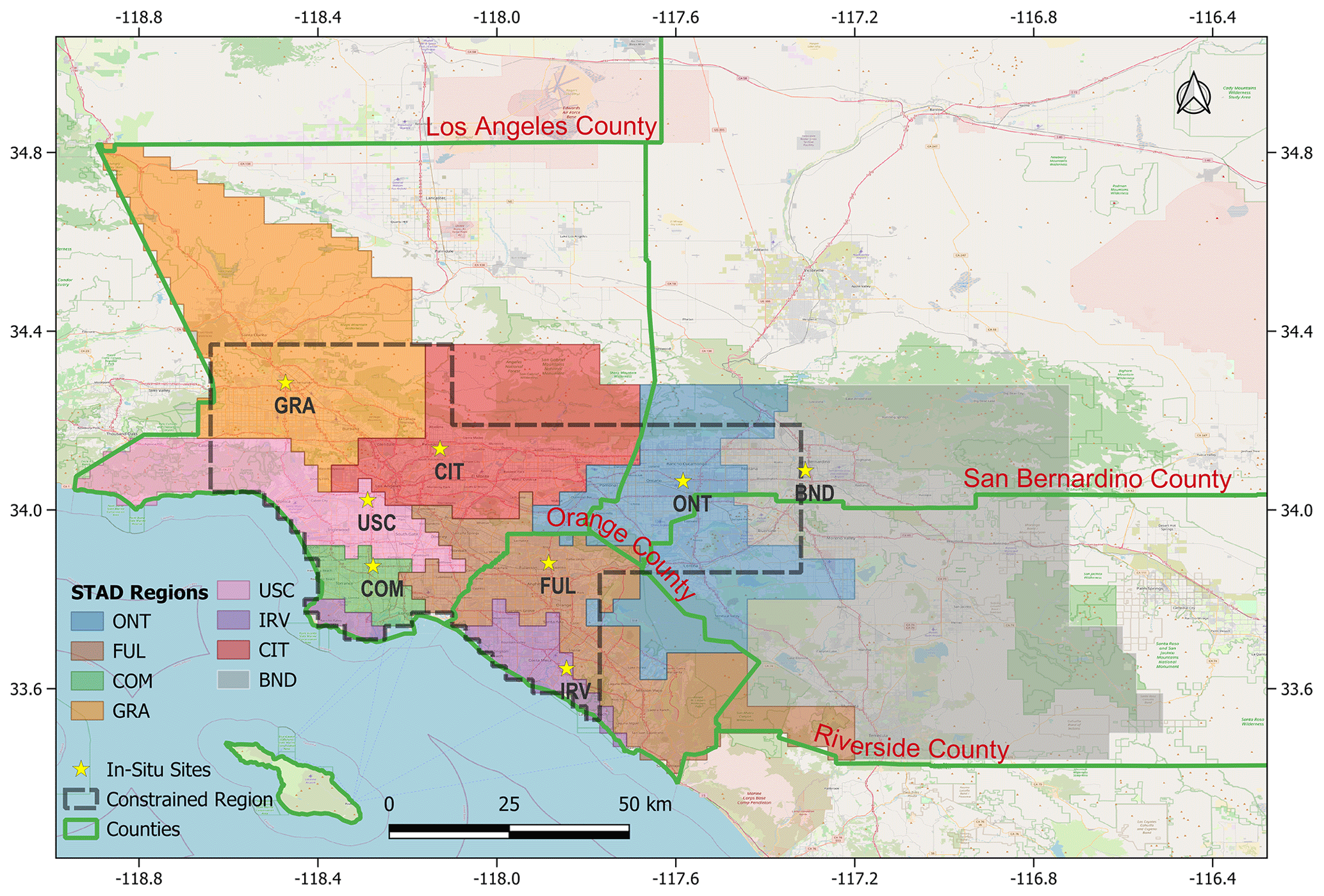
Figure 3 Study area with county boundaries, measurement locations, and the spatiotemporal area of dominance of measurement locations. The dotted black line shows the area constrained by observations, as shown in Yadav et al. (2019). Map data copyrighted by © OpenStreetMap contributors 2023. Distributed under the Open Data Commons Open Database License (ODbL) v1.0.

Overall, STAD for each site indicates the spatial regions of fluxes over a period that contribute most to the observational signal observed at a site, thus allowing us to associate the change in fluxes with the specific area in the basin for which reductions or increases in emissions are likely to have occurred. Some information in the observational signal is shared between observations from different sites. This shared information (though not shown) can be computed as part of STAD and forms part of the overall basin-scale estimates of fluxes that combine measurements from all sites. Note that STAD does not represent the network's coverage (i.e., regions of emissions constrained by observations). These regions are shorter than STAD (see the gray outline in Fig. 3). They are obtained before performing an inversion by identifying the areas of continuous spatiotemporal coverage, as provided by atmospheric transport (Fig. 4), or by assessing the model resolution after performing an inversion (for an explanation, see Yadav et al., 2019).

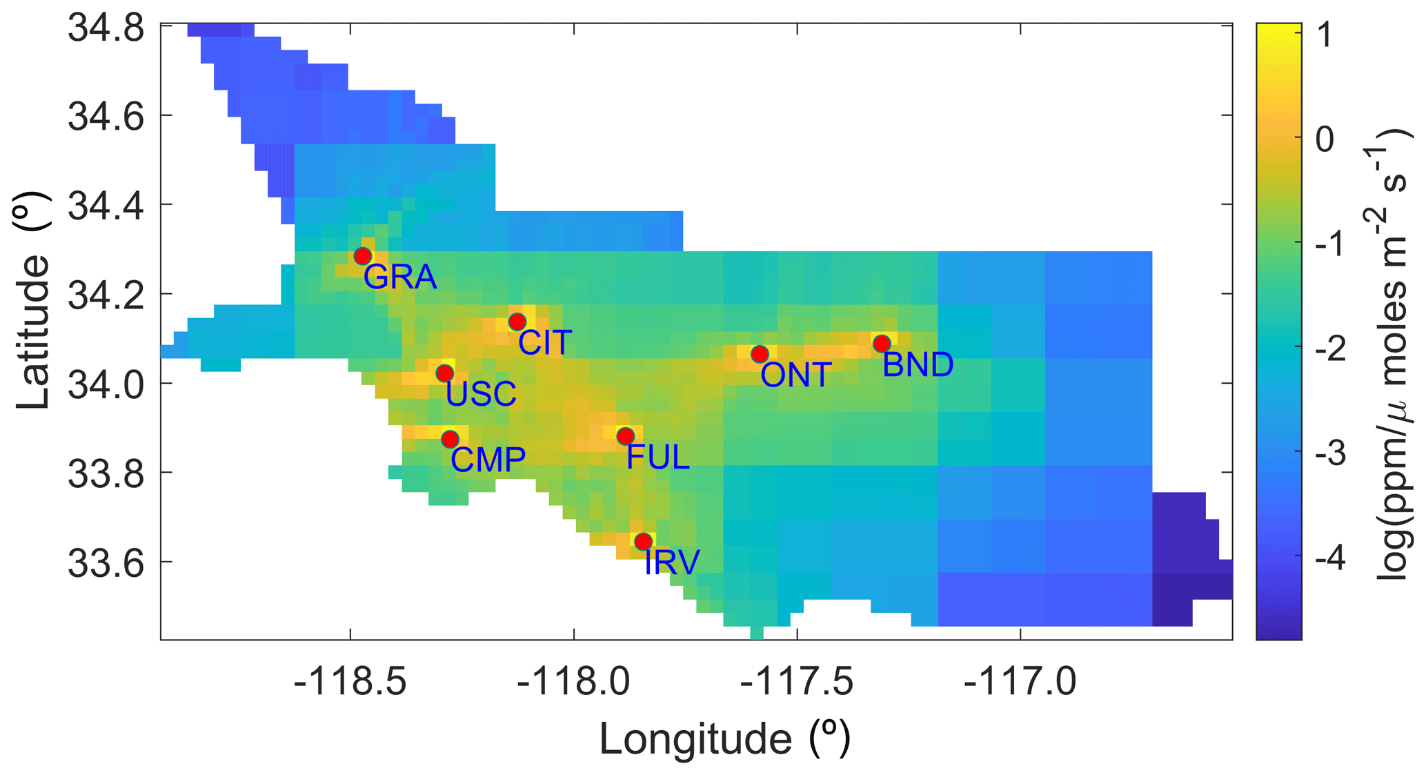
Figure 4 Heatmap of the aggregated forward operators for the case study period.

3.2 Sensitivity analysis

One of the main goals of the sensitivity analysis after performing an inversion is to identify the observations that had the most influence on the flux estimates. Other than the observations, it is also essential to explore the importance of the different input parameters to an inversion, like variance parameters in R. We describe the process of performing this analysis within the context of the case study mentioned in Sect. 3, which discusses the relative importance of the input quantities in influencing $\widehat{\mathbf{s}}$, by utilizing local sensitivities.

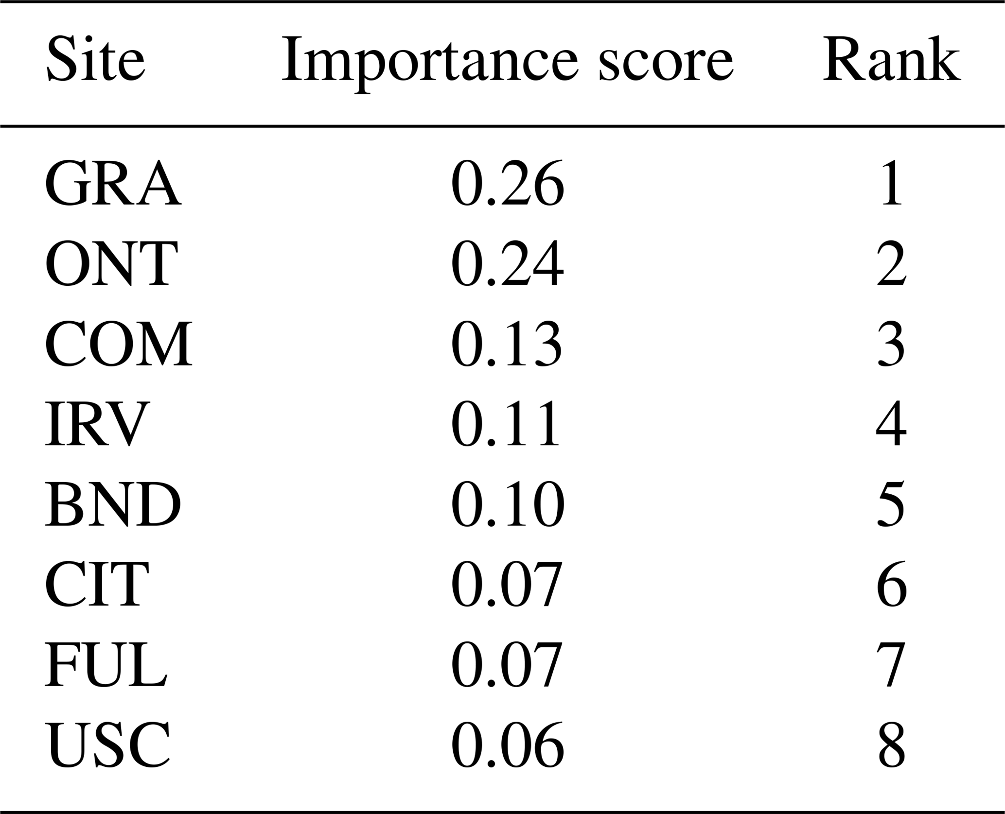
Table 1 The importance scores and ranking of eight sites based on the sensitivity of the estimated fluxes ($\widehat{\mathbf{s}}$) to observations (z).

3.2.1 Comparison and ranking of the observations

The importance of individual measurements in influencing $\widehat{\mathbf{s}}$, can be easily computed through the relative importance methodology described in Sect. 2.4. Although all entries of $\frac{\partial \widehat{\mathbf{s}}}{\partial \mathit{z}}$ are in the same units of measurement, a direct ranking of the observations or sites without employing the relative importance technique can lead to misleading results, which happens due to the presence of large negative and positive values in $\frac{\partial \widehat{\mathbf{s}}}{\partial \mathit{z}}$ that are governed by the overall spatiotemporal spread, the intensity of forward operators, and high enhancements.

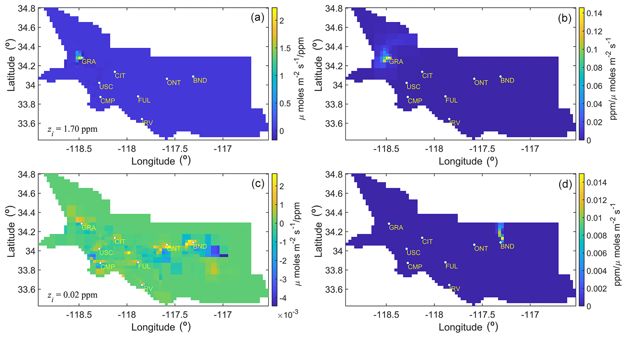
Figure 5 The sensitivities $\left(\frac{\partial \widehat{\mathbf{s}}}{\partial {\mathit{z}}_i}\right)$ and forward operators of the most and least important observations are shown here. Panels (a) and (c) depict the sensitivity of $\widehat{\mathbf{s}}$ with respect to the most (a) and least (c) important observations, respectively, during the case study period. The CH₄ enhancement corresponding to these observations is shown in the bottom-left corner of panels (a) and (c) and is denoted by the symbol z_i. Panels (b) and (d) display the forward operators associated with the sensitivities shown in panels (a) and (c), respectively.

For the case study in this work, we find that the observations collected at the GRA site that is located nearest to the source of the Aliso Canyon gas leak are most influential in governing $\widehat{\mathbf{s}}$, as shown by site-based rankings in Table 1. These rankings primarily show the importance of the observations from a site for influencing the estimated fluxes for the period under consideration and are obtained by summing the weights for each observation by employing the relative importance methodology.

Outliers have a significant impact on these rankings. The high weight associated with even one observation from a site can make that site more important compared to other sites. For example, if we remove the observation with the highest weight from each site, ONT is the most important site, followed by GRA, CMP, IRV, CIT, FUL, BND, and USC. As part of the sensitivity analysis, examining the influence of the observations associated with high weights is crucial because they are likely to have an enormous impact on the flux estimates. Site-level importance should be judged not only by examining the aggregated ranking, as presented in Table 1, but also by looking at the distribution of weights shown through the box plot in the Live Script associated with Sect. 3.2. A site with evenly distributed weights is more important than one whose importance is just due to the presence of a few observations with high weights.

The ranking of each observation in influencing the estimates of fluxes can be obtained by examining the weights of the column vectors of $\frac{\partial \widehat{\mathbf{s}}}{\partial \mathit{z}}$ and is provided in the Live Script. To exemplify, this ranking of weights showed that the observation from the GRA site with the enhancement of 1.7 ppm was most important, whereas an observation from the BND site with an enhancement of 0.02 ppm was found to be least important in influencing $\widehat{\mathbf{s}}$. Note this is not an observation with the lowest enhancement but with the least influence (Fig. 5).

3.2.2 Relative importance of $\mathbf{Q},\mathbf{R},\mathbf{X},\mathit{\beta }$ and z

After the two-step normalization of $\frac{\partial \widehat{\mathbf{s}}}{\partial \mathit{z}}$, $\frac{\partial \widehat{\mathbf{s}}}{\partial \mathbf{X}}$, $\frac{\partial \widehat{\mathbf{s}}}{\partial \mathbf{H}}$, $\frac{\partial \widehat{\mathbf{s}}}{\partial \mathit{\beta }}$, $\frac{\partial \widehat{\mathbf{s}}}{\partial \mathbf{Q}}$, and $\frac{\partial \widehat{\mathbf{s}}}{\partial \mathbf{R}}$, as described in Sect. 2.4, the spatial plots of all these grouped quantities that we call ${\frac{\partial \widehat{\mathbf{s}}}{\partial \mathit{z}}}_{\mathrm{grouped}}$,${\frac{\partial \widehat{\mathbf{s}}}{\partial \mathbf{X}}}_{\mathrm{grouped}}$, ${\frac{\partial \widehat{\mathbf{s}}}{\partial \mathbf{H}}}_{\mathrm{grouped}}$, ${\frac{\partial \widehat{\mathbf{s}}}{\partial \mathit{\beta }}}_{\mathrm{grouped}}$,${\frac{\partial \widehat{\mathbf{s}}}{\partial \mathbf{Q}}}_{\mathrm{grouped}}$, and ${\frac{\partial \widehat{\mathbf{s}}}{\partial \mathbf{R}}}_{\mathrm{grouped}}$ can be created to explore the regions of the low and high weights (see Fig. 6) at the grid scale.

Some of these quantities are correlated and should be seen in conjunction. For example, R describes the errors in z, among other errors, and implies that ${\frac{\partial \widehat{\mathbf{s}}}{\partial \mathbf{R}}}_{\mathrm{grouped}}$ and ${\frac{\partial \widehat{\mathbf{s}}}{\partial \mathit{z}}}_{\mathrm{grouped}}$ should be evaluated together to understand their importance in the influence on flux estimates. Similarly, Q describes errors in s−Xβ, implying that ${\frac{\partial \widehat{\mathbf{s}}}{\partial \mathbf{Q}}}_{\mathrm{grouped}}$ and ${\frac{\partial \widehat{\mathbf{s}}}{\partial \mathbf{X}}}_{\mathrm{grouped}}$ should be assessed together to understand their importance in the influence on flux estimates. A larger value of ${\frac{\partial \widehat{\mathbf{s}}}{\partial \mathit{z}}}_{\mathrm{grouped}}+{\frac{\partial \widehat{\mathbf{s}}}{\partial \mathbf{R}}}_{\mathrm{grouped}}$ is likely to be found around in situ sites, due to the increased model resolution. However, if ${\frac{\partial \widehat{\mathbf{s}}}{\partial \mathbf{R}}}_{\mathrm{grouped}}$ around these locations is larger in comparison to ${\frac{\partial \widehat{\mathbf{s}}}{\partial \mathit{z}}}_{\mathrm{grouped}}$, then it suggests that errors in R should be adjusted, and therefore, observations should be more important in governing the flux estimates around in situ sites. In this case study, this is due to the large variability in the enhancement caused by the Aliso Canyon gas leak and the presence of large point sources near in situ sites. Overall, for the exact location, a larger ${\frac{\partial \widehat{\mathbf{s}}}{\partial \mathit{z}}}_{{\text{grouped}}_i}$ should be accompanied by a lower ${\frac{\partial \widehat{\mathbf{s}}}{\partial \mathbf{R}}}_{{\text{grouped}}_i}$, as confirmed by the correlation in Fig. 7a and b.

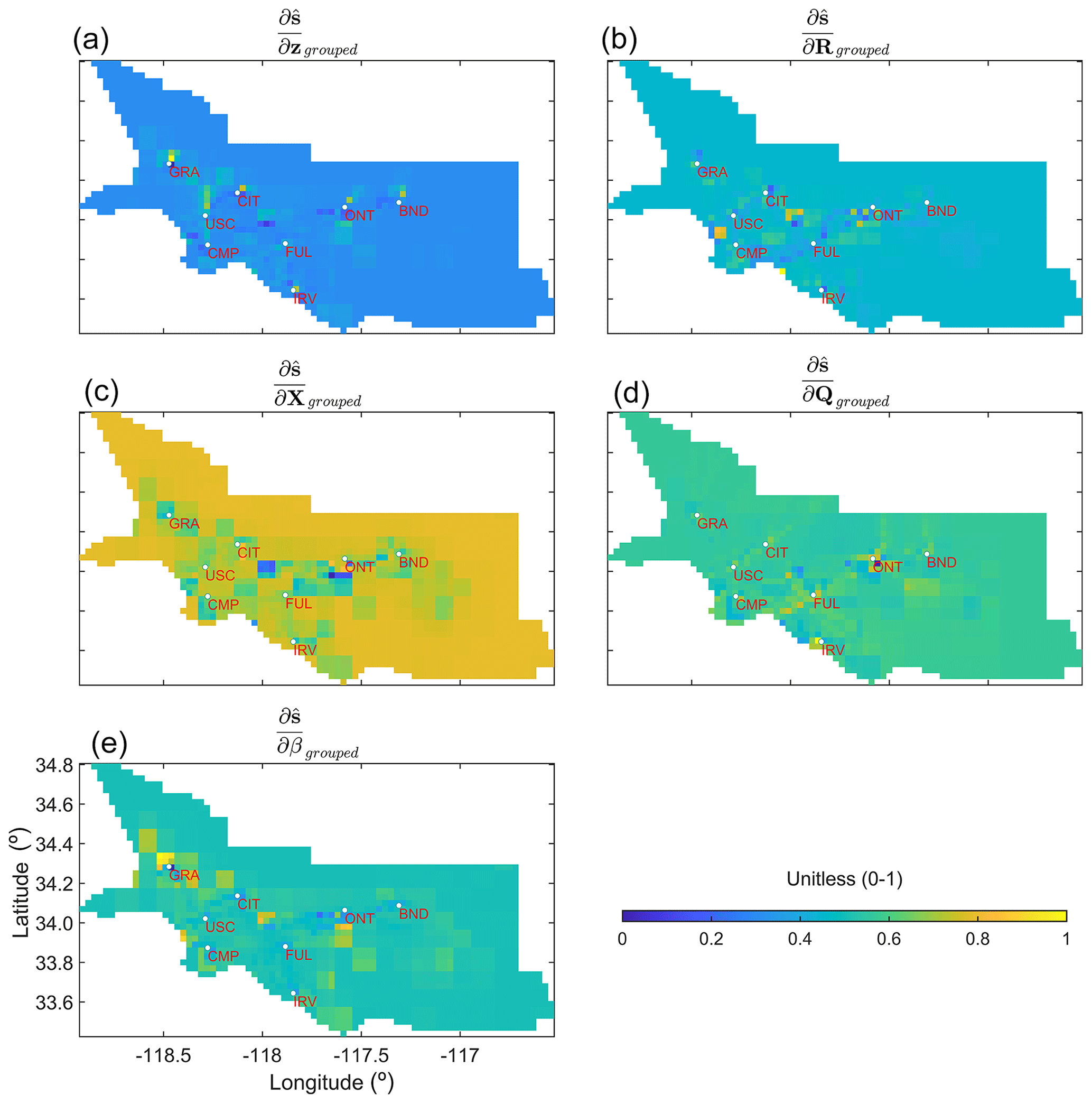
Figure 6 Grouped local sensitivities of the estimated fluxes ($\widehat{\mathbf{s}}$) with respect to z, R, X, Q, and β (from top left to bottom right, respectively). Note that, in the case of ${\frac{\partial \widehat{\mathbf{s}}}{\partial \mathit{z}}}_{\mathrm{grouped}}$, ${\frac{\partial \widehat{\mathbf{s}}}{\partial \mathbf{R}}}_{\mathrm{grouped}}$, and ${\frac{\partial \widehat{\mathbf{s}}}{\partial \mathbf{X}}}_{\mathrm{grouped}}$, a two-step normalization is performed to generate the subplots associated with these quantities. Derivatives with respect to (1) observations in z, (2) parameters in R, and (3) entries in X are normalized between 0 and 1. Then, after aggregating these for every grid cell, another min–max normalization is performed to limit their ranges between 0 and 1. Only a single normalization is performed in the case of ${\frac{\partial \widehat{\mathbf{s}}}{\partial \mathbf{Q}}}_{\mathrm{grouped}}$ and ${\frac{\partial \widehat{\mathbf{s}}}{\partial \mathit{\beta }}}_{\mathrm{grouped}}$, as they consist of only one parameter.

The increased model resolution also results in the lower importance of ${\frac{\partial \widehat{\mathbf{s}}}{\partial \mathbf{X}}}_{\mathrm{grouped}}$ and ${\frac{\partial \widehat{\mathbf{s}}}{\partial \mathbf{Q}}}_{\mathrm{grouped}}$ around sites. However, the areas unconstrained by observations are likely to have larger ${\frac{\partial \widehat{\mathbf{s}}}{\partial \mathbf{X}}}_{\mathrm{grouped}}+{\frac{\partial \widehat{\mathbf{s}}}{\partial \mathbf{Q}}}_{\mathrm{grouped}}$, as seen in Fig. 6 for ${\frac{\partial \widehat{\mathbf{s}}}{\partial \mathbf{X}}}_{\mathrm{grouped}}$ and ${\frac{\partial \widehat{\mathbf{s}}}{\partial \mathbf{Q}}}_{\mathrm{grouped}}$ quantities. If, in locations constrained by observations, ${\frac{\partial \widehat{\mathbf{s}}}{\partial \mathbf{Q}}}_{{\text{grouped}}_i}$ is larger in comparison to ${\frac{\partial \widehat{\mathbf{s}}}{\partial \mathbf{X}}}_{{\text{grouped}}_i}$, then X in these locations is incorrect and needs adjustment. Similarly, in the case of ${\frac{\partial \widehat{\mathbf{s}}}{\partial \mathbf{R}}}_{\mathrm{grouped}}$, a larger ${\frac{\partial \widehat{\mathbf{s}}}{\partial \mathbf{X}}}_{{\text{grouped}}_i}$ is generally accompanied by a lower ${\frac{\partial \widehat{\mathbf{s}}}{\partial \mathit{z}}}_{{\text{grouped}}_i}$, and vice versa, which is also visible in the correlation in Fig. 7c and d. The quantity ${\frac{\partial \widehat{\mathbf{s}}}{\partial \mathit{\beta }}}_{\mathrm{grouped}}$ provides information about the grid cells that are determining the value of $\widehat{\mathit{\beta }}$, and in this case study, as expected, this is around the Aliso Canyon gas leak for which X_i is being adjusted due to the larger flux from that region. This can also be seen in Fig. 7e, where it is positively correlated with $\widehat{\mathbf{s}}$.

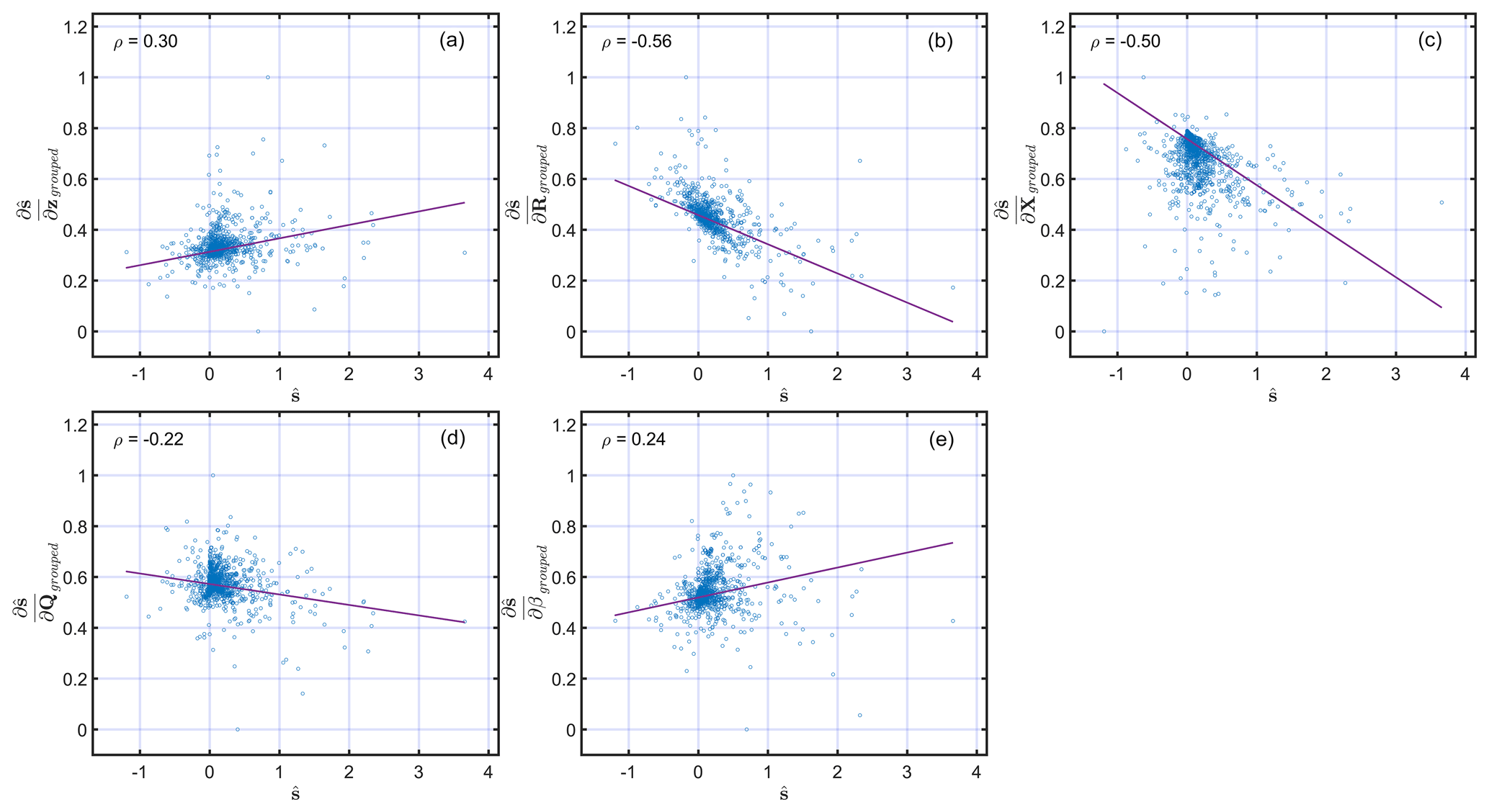
Figure 7 Scatterplots of the relationships between $\widehat{\mathbf{s}}$ and ${\frac{\partial \widehat{\mathbf{s}}}{\partial \mathbf{z}}}_{\mathrm{grouped}}$, ${\frac{\partial \widehat{\mathbf{s}}}{\partial \mathbf{R}}}_{\mathrm{grouped}}$, ${\frac{\partial \widehat{\mathbf{s}}}{\partial \mathbf{X}}}_{\mathrm{grouped}}$, ${\frac{\partial \widehat{\mathbf{s}}}{\partial \mathbf{Q}}}_{\mathrm{grouped}}$, and ${\frac{\partial \widehat{\mathbf{s}}}{\partial \mathit{\beta }}}_{\mathrm{grouped}}$. Note that, as in Fig. 6, all of the derivatives are normalized to limit their range to between 0 and 1. The correlation coefficient of the relationships shown in each scatterplot is reported in the top-left corner of the panels. The least square line of the best fit is shown with a solid red line in every panel.

4 Discussion

This study lays out the techniques for assessing the quality of the inferred estimates of fluxes. A sensitivity analysis is an important diagnostic tool for understanding the impact of the choices made with respect to input parameters on the estimated fluxes. However, it is not a recipe for selecting the proper forms of X or the structure of Q or R before performing an inversion. Other tools or methods, such as the Bayesian information criterion and variance inflation factor, should be used to perform this task.

The case study in this work is designed only to demonstrate the methodologies described in Sect. 2. We do not impose nonnegativity constraints to obtain positive CH₄ fluxes, as was done in the original 2019 study (Yadav et al., 2019). This is done because the posterior likelihood changes its functional form under nonnegativity constraints that invalidate the analytical forms of the sensitivity equations presented in this work. Thus, some CH₄ fluxes obtained in this study have negative values, as can be seen in the map of $\widehat{\mathbf{s}}$ in MATLAB's Live Script. Even in these situations, assessing sensitivity through an inversion without the imposition of nonnegativity is helpful, as it provides insights into the role of z, R, Q, and X in governing the estimates of nonnegative $\widehat{\mathbf{s}}$.

Like z, the importance of Q and R parameters can be directly obtained when all parameters have the same units of measurement, as in the case study presented in this study. However, this is not guaranteed, as R can be a function of the variance parameters and spatiotemporal correlation lengths expressed in the distance units in space and time. Furthermore, a nonstationary error covariance R can have parameters that have even more complicated units. This situation is not only limited to R but also applies to the prior error covariance, Q and X. Under these conditions, comparing the sensitivity matrices is only possible after normalization. Therefore, we recommend using a multiple linear-regression-based relative importance method to rank these quantities for comparative assessment.

The overall importance of $\frac{\partial \widehat{\mathbf{s}}}{\partial \mathit{z}}$ is best explored by performing column-based normalization and then employing the relative importance method. Additionally, column-based normalization can be augmented by row-based normalization to assess and rank the influence of observations in governing grid-scale estimates of $\widehat{\mathbf{s}}$. Qualitatively, column- and row-based assessments increase our understanding of the spatiotemporal estimates of $\widehat{\mathbf{s}}$, which is especially important when point sources are the dominant sources of emissions. Moreover, it provides insight into the temporal aggregation error (e.g., Thompson et al., 2011), as the information encoded in an instantaneous measurement can become lost over the coarser inversion period. This aggregation error also manifests spatially and is determined by the resolution at which fluxes are obtained. In many situations, these aggregation errors are unavoidable, as the choice of the spatiotemporal resolution of the inversions is governed by the density of the observations in space and time.

Other than the aggregation error, the aggregation of the estimated fluxes also has profound implications, as it affects the robustness of the estimated fluxes. It can be proved (see Appendix C1) that the aggregation of $\widehat{\mathbf{s}}$ in space and time from an inversion conducted at a finer resolution leads to a reduction in uncertainty. However, even though the ratio of the observations to the estimated fluxes increases, the number of fluxes uniquely resolved declines at a coarser resolution (see Appendix C2).

The computational cost for calculating the analytical partial derivatives is minimal, as it is a one-time operation and is bounded by the computational cost to perform matrix multiplications, which at max is O(n³). For the case study presented, we can compute the analytical derivatives and rank for approximately 4000 parameters in a few minutes on a laptop. Computing the derivatives by using the Kronecker form of the equations (Eqs. 18 and 21 through 24 and Eqs. 33 though 36) is faster for smaller problems. However, for large problems, the storage costs associated with these equations can become prohibitive. In these situations, we propose the use of the ij form of the equations (Eqs. 20 and 25 through 28 and Eqs. 29 though 32) for assessment. Furthermore, computational problems can also arise in ranking the input parameters if we have numerous derivatives (e.g., greater than 10 000), as the ranking method used in this work relies on the eigenvalue decomposition that has O(n³) computational complexity. To overcome this problem, we advise grouping the derivatives to reduce the dimension of the problem.

Finally, the estimation of STAD and the importance of sites can be influenced by data gaps; therefore, it is not advised in the presence of vast differences in the number of observations between sites.

5 Conclusions

Our work makes novel and significant contributions that can improve the understanding of linear atmospheric inverse problems. It provides (1) a framework for post hoc analysis of the impact of input parameters on the estimated fluxes and (2) a way to understand the correlations in the forward operators of an atmospheric transport model. The authors are unaware of any work in which the local sensitivities with different units of measurement are compared to rank the importance of input parameters in a linear atmospheric inverse model.

Concerning forward operators, we provide mathematical foundations for IAOMI and JSD-based metrics. These two metrics can be used to construct a nonstationary error covariance for the atmospheric transport component of the model data mismatch matrix R. Furthermore, IAOMI-based assessments can be extended to identify STAD from forward operators that can help to disaggregate the regions of influence for the observations over a chosen temporal duration. This helps us to understand the connection between the sources of flux and observations from a particular measurement location.

The IAOMI and JSD-based metrics provide essential insights into the two critical and only required components for an inversion, namely observations and forward operators (e.g., the influence of the observation on the sources of the fluxes through STAD), which can be accomplished before conducting an inversion and should be complemented by post hoc LSA, which is necessary for understanding the behavior of an inverse model. Overall, LSA can answer questions like in which locations and in what order of precedence an observation was important for the influence on the estimated fluxes. This kind of analysis is entirely different from estimating uncertainty, which tells us the prior uncertainty reduction due to observations.

LSA is not a replacement for statistical tests that check the inverse models' underlying assumptions and model specifications, nor is it a recipe for selecting input parameters to an inverse model. However, as explained above, it has an essential role that can lead to an improved understanding of an atmospheric inverse model.

Appendix A: Review of previously employed methods to conduct sensitivity analyses

Earlier, many methods have been proposed and utilized to perform sensitivity analysis. These can be categorized as global and local sensitivity analyses. Global sensitivity analysis (GSA) includes Morris's (e.g., Morris, 1991) one-step-at-a-time method (OAT), polynomial chaos expansion (PCE; e.g., Sudret, 2008), Fourier amplitude sensitivity test (FAST; e.g., Xu and Gertner, 2011), Sobol's method (e.g., Sobol, 2001), and derivative-based global sensitivity measures (DGSM; e.g., Sobol and Kucherenko, 2010), among others. These existing GSA methods (1) assume the independence of parameters (e.g., FAST and OAT), (2) are computationally expensive (e.g., Sobol's method), or (3) require knowledge of the joint probability distribution of the parameter space (e.g., DGSM and PCE). Therefore, these traditional methods cannot be directly applied to linear atmospheric inverse problems, which consist of tens of thousands of nonnormal, spatiotemporally correlated parameters (including observations). Constantine and Diaz (2017) proposed an active subspace-based GSA that uses a low-dimensional approximation of the parameter space. But it is still computationally expensive for problems with thousands of parameters (see the case study in Constantine and Diaz, 2017).

Compared to GSA, a local sensitivity method, such as Bayesian hyper-differential sensitivity analysis (HDSA; Sunseri et al., 2020), computes the partial derivatives regarding the maximum a posteriori probability (MAP) estimates of a quantity of interest. However, unlike Bayesian HDSA, we do not generate samples from the prior estimate to compute multiple MAP points, since we have limited knowledge of the prior distribution of the spatiotemporally correlated parameters. We derive the functional form of the local sensitivity equations based on the closed-form MAP solution. Our method is simple and amenable to tens of thousands of parameters. Note that, like all linear atmospheric inverse problems, one of the critical goals of this work is to study the importance of thousands of spatiotemporally varying parameters by ranking them, and the computation of the local sensitivities is a means to achieve that goal.

Appendix B: Jensen–Shannon distance (JSD) for forward operators

The dissimilarity between forward operators can also be measured via entropy-based distances (for a definition, see MacKay, 2003), which can capture differences between two probability distributions. One such metric is the Jensen–Shannon distance (JSD; Nielsen, 2019), which can be used to compute the distance between two forward operators after normalizing them by their total sum. For a forward operator F, this can be given as

$$\begin{array}{}\text{(B1)}& P_{F_k}={\displaystyle \frac{F_k}{{\sum }_k{F}_k}},\end{array}$$

where F_k denotes kth entry of F, resulting in the normalized forward operator P. We can then use JSD to compute the distance between two normalized forward operators from Eq. (B2) as follows:

$$\begin{array}{}\text{(B2)}& \text{JSD}\left(P_{\mathbf{F}}\mathrm{|}\mathrm{|}{P}_{\mathbf{G}}\right)=\sqrt{{\displaystyle \frac{\mathrm{1}}{\mathrm{2}}}D\left(P_{\mathbf{F}}\mathrm{|}\mathrm{|}M\right)+{\displaystyle \frac{\mathrm{1}}{\mathrm{2}}}D\left(P_{\mathbf{G}}\mathrm{|}\mathrm{|}M\right),}\end{array}$$

where D stands for the Kullback–Leibler (KL) divergence (see MacKay, 2003, for details). The KL divergence D of any probability distribution p, with respect to another probability distribution q, is defined as $D\left(p\mathrm{|}\mathrm{|}q\right)=\sum p\text{log}(p/q)$, and M stands for $\frac{\mathrm{1}}{\mathrm{2}}\left(P_{\mathbf{F}}+P_{\mathbf{G}}\right)$. The symbol || is used to indicate that D(P_F||M) and D(P_G||M) are not conditional entropies (see MacKay, 2003). JSD is closed and bounded in [0,1] when the KL divergence is calculated with the base 2 logarithms. Intuitively, JSD and 1−ν (i.e., 1− IAOMI) are comparable, since both of them are measures of dissimilarity.

Appendix C: Uncertainty and model resolution under aggregation

Here we show the proofs of two mathematical statements on the robustness and quality of the estimated fluxes, as mentioned in Sect. 4. First, we show why the marginal variance of the estimated fluxes (which is the diagonal of the covariance matrix of $\widehat{\mathbf{s}}$) decreases when the estimated fluxes are post-aggregated to a coarser scale or upscaled (Appendix C1). Second, we show why, in such cases, the model resolution (termed the total information resolved by the observations) also decreases (Appendix C2). Note that the nomenclature used in the Appendix C should not be confused with the nomenclature introduced in Sect. 2. The abbreviations and symbols used here are independent of what is used in Sect. 2.

C1 Proof of the reduction in the marginal variance of $\widehat{\mathbf{s}}$ when aggregation is performed

The post-inversion aggregation or upscaling of any flux field s is equivalent to the pre-multiplication by a weight matrix (in fact, a row stochastic matrix). This can be written as follows:

$$\begin{array}{}\text{(C1)}& \stackrel{\mathrm{̃}}{\mathbf{s}}=\mathbf{J}\widehat{\mathbf{s}},\end{array}$$

where J is a row stochastic (i.e., row sums are all unity) k×m weight matrix (k<m). The variance of $\stackrel{\mathrm{̃}}{\mathbf{s}}$ can be written as JΣJ^t, where var$\left(\stackrel{\mathrm{̃}}{\mathbf{s}}\right)=\mathbf{J}\text{var}\left(\widehat{\mathbf{s}}\right)J^t=\mathbf{J}\mathbf{\Sigma }{\mathbf{J}}^t$. The general structure of J is as follows:

$$\begin{array}{}\text{(C2)}& J=\left[\begin{array}{cccccc}\mathrm{0}& j_{\mathrm{12}}& j_{\mathrm{13}}& \mathbf{0}& \mathbf{0}& \mathbf{0}\\ j_{\mathrm{21}}& \mathbf{0}& j_{\mathrm{2}r+\mathrm{1}}& j_{\mathrm{2}r+\mathrm{2}}& \mathbf{0}& \mathbf{0}\\ \mathrm{⋮}& \mathrm{⋮}& \mathrm{\ddots }& \mathrm{\ddots }& \mathrm{⋮}& \mathrm{⋮}\\ \mathbf{0}& \mathbf{0}& \mathbf{0}& j_{km}& \mathbf{0}& \mathbf{0}\end{array}\right]=\left[\begin{array}{c}{\mathbf{j}}_{\mathrm{1}}^t\\ {\mathbf{j}}_{\mathrm{2}}^t\\ \mathrm{⋮}\\ {\mathbf{j}}_k^t\end{array}\right].\end{array}$$

However, J is mostly sparse, with nonzero values in only a few places. The rest of the entries are zeros. Essentially, J can have any number of nonzero entries in a row that may or may not be consecutive. This is because, although adjacent grids are averaged on a map, they may not be adjacent upon vectorization. Moreover, the geometry of the map may not be exactly square or rectangular. Therefore, depending on the aggregation or upscaling factor and geometry, there may or may not be any neighboring grid for averaging around a particular grid. However, the rows are linearly independent, as nearby grids are considered only once for averaging. The properties of J are as follows:

1. J1=1 or ${\mathbf{j}}_i^t\mathbf{1}=\mathrm{1}\forall i=\mathrm{1},\mathrm{2},\cdot ,\cdot ,k$

2. ${\mathbf{j}}_i^t{\mathbf{j}}_r=\mathrm{0}$   for   i≠r.

We can rearrange the columns of J and the rows of Σ accordingly without the loss of any structure, such that nonzero entries are consecutive for each row of J. The matrix JΣJ^′ under the column permutation can be written as follows:

$$\begin{array}{}\text{(C3)}& {\displaystyle }\begin{array}{rl}\mathbf{J}\mathbf{\Sigma }{\mathbf{J}}^{\mathbf{t}}& ={\mathbf{J}}_{\mathit{\pi }}{\mathbf{\Sigma }}_{\mathit{\pi }}{\mathbf{J}}_{\mathit{\pi }}^t\\ & ={\left[\begin{array}{cccc}{\mathbf{l}}_{\mathrm{1}}^t& \mathrm{0}& \mathrm{\cdots }& \mathrm{0}\\ \mathrm{0}& {\mathbf{l}}_{\mathrm{2}}^t& \mathrm{\cdots }& \mathrm{0}\\ \mathrm{⋮}& \mathrm{⋮}& \mathrm{\ddots }& \mathrm{⋮}\\ \mathrm{0}& \mathrm{0}& \mathrm{\cdots }& {\mathbf{l}}_k^t\end{array}\right]}_{k\times m}{\left[\begin{array}{cccc}{\mathbf{\Xi }}_{\mathrm{11}}& {\mathbf{\Xi }}_{\mathrm{12}}& \mathrm{\cdots }& {\mathbf{\Xi }}_{\mathrm{1}k}\\ {\mathbf{\Xi }}_{\mathrm{21}}& {\mathbf{\Xi }}_{\mathrm{22}}& \mathrm{\cdots }& \mathrm{⋮}\\ \mathrm{⋮}& \mathrm{⋮}& \mathrm{\ddots }& \mathrm{⋮}\\ {\mathbf{\Xi }}_{k\mathrm{1}}& \mathrm{⋮}& \mathrm{\dots }& {\mathbf{\Xi }}_{kk}\end{array}\right]}_{m\times m}\\ & {\left[\begin{array}{cccc}{\mathbf{l}}_{\mathrm{1}}& \mathrm{0}& \mathrm{\cdots }& \mathrm{0}\\ \mathrm{0}& {\mathbf{l}}_{\mathrm{2}}& \mathrm{\cdots }& \mathrm{0}\\ \mathrm{⋮}& \mathrm{⋮}& \mathrm{\ddots }& \mathrm{⋮}\\ \mathrm{0}& \mathrm{0}& \mathrm{\cdots }& {\mathbf{l}}_k\end{array}\right]}_{p\times k}\end{array}\text{(C4)}& {\displaystyle }={\left[\begin{array}{ccc}{\mathbf{l}}_{\mathrm{1}}^t{\mathbf{\Xi }}_{\mathrm{11}}{\mathbf{l}}_{\mathrm{1}}& \mathrm{\dots }& {\mathbf{l}}_{\mathrm{1}}^t{\mathbf{\Xi }}_{\mathrm{1}k}{\mathbf{l}}_k\\ \mathrm{⋮}& {\mathbf{l}}_{\mathrm{2}}^t{\mathbf{\Xi }}_{\mathrm{22}}{\mathbf{l}}_{\mathrm{2}}& \mathrm{\cdots }\\ {\mathbf{l}}_k^t{\mathbf{\Xi }}_{k\mathrm{1}}{\mathbf{l}}_{\mathrm{1}}& \mathrm{\cdots }& {\mathbf{l}}_k^t{\mathbf{\Xi }}_{kk}{\mathbf{l}}_k\end{array}\right]}_{k\times k},\end{array}$$

where J_π and Σ_π are the permuted J and Σ, respectively. However, for notational clarity, we use l and Ξ as the sub-vector and sub-block matrix of the J_π and Σ_π, respectively. Note that any ${\mathbf{l}}_i^t$ is a row vector with the dimension of (1,d_i), and Ξ_ii is a square matrix with the dimension of (d_i,d_i), where ${\sum }_{i=\mathrm{1}}^k{d}_i=m$. Thus, the diagonal entry ${\mathbf{l}}_i^t{\mathbf{\Xi }}_{ii}{\mathbf{l}}_i$ is a scalar quantity. For any ith diagonal entry, the corresponding scalar quantity can be written as ∑_jrll_ijl_irΞ_jr. Through symmetry of Ξ, this reduces to the following:

$$\begin{array}{}\text{(C5)}& {\mathbf{l}}_i^t{\mathbf{\Xi }}_{ii}{\mathbf{l}}_i=\sum _r{l}_{ir}^{\mathrm{2}}{\mathrm{\Xi }}_{lr}^{\mathrm{2}}+\mathrm{2}\sum _{j>r}{l}_{ij}{l}_{ir}{\mathrm{\Xi }}_{jr}.\end{array}$$

Using the Cauchy–Schwarz inequality on Ξ_jr, this can be written as

$$\begin{array}{}\text{(C6)}& {\displaystyle }\begin{array}{rl}\sum _r{l}_{ir}^{\mathrm{2}}{\mathit{\sigma }}_{lr}^{\mathrm{2}}& -\mathrm{2}\sum _{j>r}{l}_{ij}{l}_{ir}{\mathit{\sigma }}_{jj}{\mathit{\sigma }}_{rr}\le \sum _r{l}_{ir}^{\mathrm{2}}{\mathit{\sigma }}_{rr}^{\mathrm{2}}\\ & +\mathrm{2}\sum _{j>r}{l}_{ij}{l}_{ij}{\mathit{\sigma }}_{jr}\le \sum _r{l}_{ir}^{\mathrm{2}}{\mathit{\sigma }}_{rr}^{\mathrm{2}}\\ & +\mathrm{2}\sum _{j>r}{l}_{ij}{l}_{ij}{\mathit{\sigma }}_{jj}{\mathit{\sigma }}_{rr}\end{array}\text{(C7)}& {\displaystyle }\begin{array}{rl}{\left(l_{ir}\sqrt{{\mathit{\sigma }}_{ir}}-\sum _{r\ge \mathrm{2}}{l}_{ir}\sqrt{{\mathit{\sigma }}_{ir}}\right)}^{\mathrm{2}}& \le \sum _r{l}_{ir}^{\mathrm{2}}{\mathit{\sigma }}_{rr}^{\mathrm{2}}+\mathrm{2}\sum _{j>r}{l}_{ij}{l}_{ij}{\mathit{\sigma }}_{jj}{\mathit{\sigma }}_{rr}\\ & \le {\left(\sum _{ir}{l}_{ir}\sqrt{{\mathit{\sigma }}_{rr}}\right)}^{\mathrm{2}}\end{array}\text{(C8)}& {\displaystyle }\begin{array}{rl}{\text{min}}_r{\mathit{\sigma }}_{rr}{\left(l_{ir}-\sum _{r\ge \mathrm{2}}{l}_{ir}\right)}^{\mathrm{2}}& \le \sum _r{l}_{ir}^{\mathrm{2}}{\mathit{\sigma }}_{rr}^{\mathrm{2}}+\mathrm{2}\sum _{j>r}{l}_{ij}{l}_{ij}{\mathit{\sigma }}_{jj}{\mathit{\sigma }}_{rr}\\ & \le {\text{max}}_r{\mathit{\sigma }}_{rr}{\left(\sum _{ir}{l}_{ir}\right)}^{\mathrm{2}}.\end{array}\end{array}$$

This implies (by property 1 of the weight matrix J) that the ith diagonal entry is bounded by the following:

$$\begin{array}{}\text{(C9)}& \underset{r}{min}{\mathit{\sigma }}_{rr}{\left(l_{ir}-\sum _{r\ge \mathrm{2}}{l}_{ir}\right)}^{\mathrm{2}}\le {\mathbf{J}}_{\mathbf{i}}^{\prime }{\mathbf{\Sigma }}_{\mathbf{ii}}{\mathbf{J}}_{\mathbf{i}}\le \underset{r}{max}{\mathit{\sigma }}_{rr}\le \sum _{r=\mathrm{1}}^{d_i}{\mathit{\sigma }}_{rr},\end{array}$$

where ${\sum }_{r=\mathrm{1}}^{d_i}{\mathit{\sigma }}_{rr}$ is the sum of the marginal variance of the ith block of the non-averaged $\widehat{\mathbf{s}}$. Thus, the sum of the marginal variance of $\stackrel{\mathrm{̃}}{\mathbf{s}}$, which is the sum of the i diagonal ${\mathbf{J}}_i^t{\mathbf{\Sigma }}_{ii}{\mathbf{J}}_i$, is also smaller than or equal to the sum total of marginal variance of $\widehat{\mathbf{s}}$. This implies that the marginal variance of the posterior mean decreases as a result of the diagonal of the variance matrix shrinking in magnitude upon averaging.

C2 Proof of the reduction in model resolution when aggregation is performed

The aggregated forward operator $\stackrel{\mathrm{̃}}{\mathbf{H}}$ can be written as follows:

$$\begin{array}{}\text{(C10)}& \stackrel{\mathrm{̃}}{\mathbf{H}}=\mathbf{HB},\end{array}$$

where B is the upscaling matrix. The dimension of B has the dimension of the transpose of J. The structural form of B is similar to the form of J explained in Eq. (C2). Nonzero entries of B are in the same place as J^′, with the magnitude replaced by unity. This is evident from the fact that the forward operator is summed instead of being averaged for aggregation. The properties of B are as follows:

1. B1=1.

2. $\mathbf{JB}=\text{diag}(\mathit{N}{)}^{k\times k}$,    where N is the vector of the number of neighboring grid cells for any particular grid cell, i.e., $\mathit{N}=\left(N_{\mathrm{1}},\mathrm{\dots },N_k\right)$.

3. $\mathbf{BJ}={\left[\begin{array}{cccc}{\mathbf{C}}_{\mathbf{1}}& \mathbf{0}& \mathrm{\cdots }& \mathbf{0}\\ \mathbf{0}& {\mathbf{C}}_{\mathbf{2}}& \mathrm{\cdots }& \mathbf{0}\\ \mathrm{⋮}& \mathrm{⋮}& \mathrm{\ddots }& \mathrm{⋮}\\ \mathbf{0}& \mathrm{⋮}& \mathrm{\cdots }& {\mathbf{C}}_{\mathbf{k}}\end{array}\right]}^{m\times m}$
   is a block diagonal matrix. Any block C_i of JA can be expressed as a varying dimension (depending on the number of neighboring grids of any particular grid cell) matrix of the following form:

   $$\begin{array}{}\text{(C11)}& {\mathbf{C}}_i={\left[\begin{array}{ccc}\frac{\mathrm{1}}{N_i}& \mathrm{\cdots }& \frac{\mathrm{1}}{N_i}\\ \mathrm{⋮}& \mathrm{\ddots }& \mathrm{⋮}\\ \frac{\mathrm{1}}{N_i}& \mathrm{\cdots }& \frac{\mathrm{1}}{N_i}\end{array}\right]}^{N_i\times N_i}={\displaystyle \frac{\mathrm{1}}{N_i}}{\mathbf{11}}^t.\end{array}$$

4. BJ is symmetric and positive semi-definite.

The first three properties are simple observations from the construction. So, here we provide proof of the fourth property.

Proof. By construction, $\text{Det}(\mathbf{BJ}-\mathit{\lambda }\mathbf{I})=\text{Det}({\mathbf{C}}_{\mathbf{1}}-\mathit{\lambda }\mathbf{I})\mathrm{\dots }\text{Det}({\mathbf{C}}_{\mathbf{k}}-\mathit{\lambda }\mathbf{I})$. So, eigenvalues of BJ are the list of the eigenvalues of the block matrices. It can be proved that 1 and 0 are the only two distinct eigenvalues of C_i for any i. Below is a brief argument on that topic, where $\left(\frac{\mathrm{1}}{N_i}{\mathbf{11}}^t\right)\mathbf{1}=\frac{\mathrm{1}}{N_i}\mathbf{1}{N}_i=\mathrm{1}\cdot \mathbf{1}$ implies that one eigenvalue of C_i is 1. Observe that $\text{rank}\left(\frac{\mathrm{1}}{N_i}{\mathbf{11}}^t\right)=\text{rank}\left(\mathbf{1}\right)=\mathrm{1}$. Hence, the dimension of the null space $\text{dim}\left(\mathcal{N}\left(\frac{\mathrm{1}}{N_i}{\mathbf{11}}^t\right)\right)=k-\text{rank}\left(\frac{\mathrm{1}}{N_i}{\mathbf{11}}^t\right)=k-\mathrm{1}$. This implies that the other eigenvalue of C_i is 0, with multiplicity of k−1.

So, not only is C_i symmetric but also the eigenvalues of C_i are always nonnegative. Consequently, all eigenvalues of BJ are of a similar form i.e., BJ is a symmetric positive semi-definite.

Finally, the model resolution matrix for the inversion can be written as $\frac{\partial \widehat{\mathbf{s}}}{\partial \mathbf{z}}\mathbf{H}$, where H is the forward operator. The post-inversion aggregated model resolution can be written as

$$\begin{array}{}\text{(C12)}& {\displaystyle \frac{\partial \stackrel{\mathrm{̃}}{\mathbf{s}}}{\partial \mathbf{z}}}\stackrel{\mathrm{̃}}{\mathbf{H}}=\mathbf{A}{\displaystyle \frac{\partial \widehat{\mathbf{s}}}{\partial \mathbf{z}}}\mathbf{HB}\end{array}$$

by Eqs. (C1) and (C10).

The question is then as follows: what happens to the trace of the model resolution under the aggregated scenario? We provide proof for the simple batch Bayesian case in Lemma 1. The proof for the geostatistical case is similar and is left to the enthusiastic reader.

Lemma 1.

$$\begin{array}{}\text{(C13)}& \begin{array}{c}\mathbf{Mres}={\mathbf{QH}}^{\prime }{\mathit{\psi }}^{-\mathbf{1}}H\\ {\mathbf{Mres}}_{\mathrm{aggregated}}={\mathbf{JQH}}^{\prime }{\mathit{\psi }}^{-\mathbf{1}}HB\text{then}\\ \text{trace}\left({\mathbf{Mres}}_{\mathrm{aggregated}}\right)\le \text{trace}\left(\mathbf{Mres}\right)\end{array}\end{array}$$

Proof. The model resolution for the aggregated scenario can be written as follows:

$$\begin{array}{}\text{(C14)}& \begin{array}{rl}& \text{trace}\left({\mathbf{Mres}}_{\mathrm{aggregated}}\right)=\text{trace}\left({\mathbf{JQH}}^{\prime }{\mathit{\psi }}^{-\mathbf{1}}HB\right)\\ & =\text{trace}\left({\mathbf{BJQH}}^{\prime }{\mathit{\psi }}^{-\mathbf{1}}H\right)=\text{trace}\left(\mathbf{WS}\right),\\ & \text{where}\mathbf{W}=\mathbf{BJ},\mathbf{S}={\mathbf{QH}}^{\prime }{\mathit{\psi }}^{-\mathbf{1}}H,\end{array}\end{array}$$

where S and W are both of the dimension of (m×m). S is a positive semi-definite matrix, since both Q and ${\mathbf{H}}^{\prime }{\mathit{\psi }}^{-\mathbf{1}}H$ are positive semi-definite. For the W^m×m and S^m×m positive semi-definite, the trace of their product can be bounded by the following quantities (see Kleinman and Athans, 1968, and the discussion in Fang et al., 1994):

$$\begin{array}{}\text{(C15)}& {\mathit{\lambda }}_{min}\left(\mathbf{W}\right)\text{trace}\left(\mathbf{S}\right)\le \text{trace}\left(\mathbf{WS}\right)\le {\mathit{\lambda }}_{min}\left(\mathbf{W}\right)\text{trace}\left(\mathbf{S}\right).\end{array}$$

From property 4 of the weight matrix B, we know that ${\mathit{\lambda }}_{min}\left(\mathbf{W}\right)=\mathrm{0}$ and ${\mathit{\lambda }}_{max}\left(\mathbf{W}\right)=\mathrm{1}$; hence, the above reduces to $\mathrm{0}\le \text{trace}\left(\mathbf{WS}\right)\le \mathrm{1}\cdot \text{trace}\left(\mathbf{S}\right)$. Therefore, the proof by Eq. (C14) can be seen.