The High-resolution Intermediate Complexity Atmospheric Research (HICAR v1.1) model enables fast dynamic downscaling to the hectometer scale

High-resolution (< 1 km) atmospheric modeling is increasingly used to study precipitation distributions in complex terrain and cryosphere–atmospheric processes. While this approach has yielded insightful results, studies over annual timescales or at the spatial extents of watersheds remain unrealistic due to the computational costs of running most atmospheric models. In this paper we introduce a high-resolution variant of the Intermediate Complexity Atmospheric Research (ICAR) model, HICAR. We detail the model development that enabled HICAR simulations at the hectometer scale, including changes to the advection scheme and the wind solver. The latter uses near-surface terrain parameters which allow HICAR to simulate complex topographic flow features. These model improvements clearly influence precipitation distributions at the ridge scale (50 m), suggesting that HICAR can approximate processes dependent on particle–flow interactions such as preferential deposition. A 250 m HICAR simulation over most of the Swiss Alps also shows monthly precipitation patterns similar to two different gridded precipitation products which assimilate available observations. Benchmarking runs show that HICAR uses 594 times fewer computational resources than the Weather Research and Forecasting (WRF) atmospheric model. This gain in efficiency makes dynamic downscaling accessible to ecohydrological research, where downscaled data are often required at hectometer resolution for whole basins at seasonal timescales. These results motivate further development of HICAR, including refinement of parameterizations used in the wind solver and coupling of the model with an intermediate-complexity snow model.

1 Introduction

Atmospheric models have seen remarkable improvements over the past decades, spurred on by their importance to society. Their usage within science ranges from climate and weather predictions to downscaling atmospheric variables as input to further geophysical models. Specific applications have included generating forcing data over sparsely instrumented domains (Khadka et al., 2022), downscaling global climate model output to study regional impacts (Spinoni et al., 2018), and coupling with land surface models to better simulate land–atmosphere feedbacks (Sharma et al., 2023). The concept intrinsic to all of these applications is one of scale. As model resolution increases, processes which were previously parameterized can be explicitly resolved, and the representation of the underlying terrain improves, allowing for more accurate dynamics (Wyngaard, 2004; Chow et al., 2019; Prein et al., 2013).

High-resolution (< 1 km) simulations of winter storms in complex terrain have been used to augment our process-level understanding of particle–flow interactions such as preferential deposition (Lehning et al., 2008; Gerber et al., 2018; Vionnet et al., 2017; Mott et al., 2010). Some of these simulations aimed at very high resolutions of 25 m and below and thus used stationary wind fields (Raderschall et al., 2008) or a decomposition of wind field into a limited number of dominating (stationary) patterns to enable simulations for the length of a storm (Mott et al., 2010) to a full season (Groot Zwaaftink et al., 2013). Coupled glacier–atmosphere models have been developed and run at a range of spatial scales, demonstrating an ability to better simulate surface–atmosphere energy exchanges over glaciers (Collier et al., 2013; Goger et al., 2022). And coupled snow–atmosphere models have been developed which explicitly resolve snow–atmosphere interactions (Vionnet et al., 2014; Sharma et al., 2023). These studies have all demonstrated the ability of high-resolution atmospheric modeling to improve estimates of precipitation, wind speeds, and surface–atmosphere interactions. However, all of them have focused on limited spatial and temporal extents due to the huge computational demand required for running modern atmospheric models at hectometer resolution. In one study performing 50 m simulations of winter precipitation using the Weather Research and Forecasting (WRF) model, nearly 34 000 core hours were required to perform 1 d of simulation over a < 100 km² domain (Kruyt et al., 2022). Any practical application of high-resolution atmospheric modeling to questions concerning future climate scenarios or downscaling for land surface models is currently limited by the computational demand of atmospheric models.

This issue is no news to the community, and idealized atmospheric models of orographic precipitation and mountain waves have been developed and employed in the past (Smith, 1979; Smith and Barstad, 2004). Recently, the Intermediate Complexity Atmospheric Research (ICAR) model was introduced in Gutmann et al. (2016) (hereafter G16) to provide an alternative to highly idealized models and modern, nonhydrostatic, compressible atmospheric models. In their 2016 paper, Gutmann et al. demonstrated excellent agreement between ICAR and WRF when simulating mountain waves and orographic precipitation over idealized terrain. Further demonstration over real, complex terrain at a 4 km resolution gave good agreement on precipitation between the two models during the winter months. Most importantly, the ICAR simulations used 143 times fewer computational resources than the WRF model. The ability of ICAR to simulate orographic precipitation at the kilometer scale has been replicated in other studies (Horak et al., 2019). ICAR has since occupied a niche in modeling studies where downscaling of long time series would otherwise be limited by computational resources. These results motivate the design philosophy behind ICAR that dramatic reductions in computational time may justify modest reductions in model accuracy for certain applications.

Such an approach is perfectly suited for high-resolution atmospheric modeling, where computational demands severely limit the experimental design of studies. However, the dynamics and physics of the base ICAR model, namely linear mountain wave theory and first-order upwind advection, are not suitable when modeling at the hectometer scale. Here we introduce a high-resolution variant of the ICAR model, HICAR, which adapts the ICAR model to be suitable at resolutions below the kilometer scale. In the second section of the paper, key parts of HICAR's model development are detailed, with a focus on the model's wind solver, advection scheme, and input/output (I/O) operations. In the third section, information is given about other atmospheric models and gridded datasets used in this study, as well as details about model simulation setups. These models and datasets are then compared in Sect. 4, where various demonstrations of the HICAR model provide a limited validation and are used to discuss the model performance. Lastly, a synthesis of the paper and a concluding discussion about the utility of the HICAR model are presented in Sect. 5.

2 Model development

In the original ICAR model, the 3D wind field can either be generated through 3D interpolation between the coarse-resolution forcing data and the high-resolution grid, or it can be further modified using linear mountain wave theory (Smith, 1979). This modification alone simulates the disturbance of the mesoscale flow field caused by mountain ranges, namely the generation of mountain waves depending on the atmospheric stability. These effects are the dominant influence of the terrain on the mesoscale flow from scales of tens of kilometers down to the kilometer scale, which is the scale range which ICAR was originally developed for. Increasingly, output from kilometer-scale compressible, nonhydrostatic atmospheric models run by regional weather forecasting offices are available (Benjamin et al., 2016; Seifert et al., 2008; Seity et al., 2011). These models are expected to capture the dynamics approximated by linear mountain wave theory. When using these models as forcing data for high-resolution simulations with ICAR, it would thus be redundant to run with the linear theory solution. Left with only an interpolated kilometer-scale wind field for a 3D wind field, we found it necessary to implement a new wind solver capable of capturing dynamics induced by the underlying high-resolution terrain. These flow features should be necessary to simulate particle–flow interactions which lead to heterogeneous snowfall patterns. In addition to changes to the wind field, it was also necessary to modify the advection scheme of ICAR and the input/output (I/O) routines. ICAR only offers the first-order upwind advection scheme, which has been shown to be highly diffusive, especially in complex terrain (Schär et al., 2002). When simulating precipitation events, it is important that heterogeneities in moisture and temperature are maintained and do not become too smooth. Finally, as model resolution and speed increased, it became paramount to be able to efficiently read and write large volumes of data without significantly affecting runtime. The following two subsections focus on new options for the wind solver in HICAR, while the last two focus on changes affecting the advection scheme and model input/output (I/O) (Fig. 1).

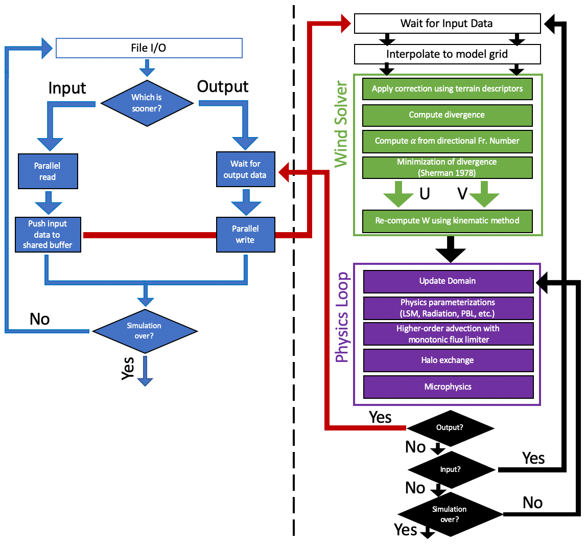
Figure 1 Schematic of major changes to HICAR's runtime loop compared to Fig. 1 of G16. The left side of the figure features the I/O loop handled by I/O processes, while the right side features the runtime loop of HICAR, with a focus on the steps discussed in Sect. 2.2 and 2.3. Blue corresponds to I/O processes, green to steps of the wind solver, purple to  steps of the physics integration loop, and red to communication between I/O and compute processes. Within the wind solver and physics loop, downward arrows are implied between the steps where not indicated.

2.1 Direct adjustment of wind field

Taking a cue from existing statistical models of surface winds in complex terrain (Winstral and Marks, 2002; Winstral et al., 2017; Liston and Elder, 2006; Dujardin and Lehning, 2022), we first develop corrections to the interpolated wind field near the surface based on the underlying terrain. This is done through terrain descriptors calculated at model initialization and then applied to the wind field at runtime. Terrain descriptors represent some qualitative information about the terrain quantitatively, such as if a particular location is sheltered from a particular wind direction. Parameterizations can then be developed using these values, allowing nonlocal interactions between the topography and winds to be accounted for in a computationally efficient manner.

2.1.1 Terrain descriptors

Topographic position index (TPI)

When downscaling winds from coarse to high resolutions, the representation of the model terrain can vary drastically. What appears as a small depression in the terrain at a 1 km resolution may actually be a steep valley when viewed at a 100 m resolution. To find areas in the high-resolution domain where large differences with the coarse digital elevation model (DEM) may affect wind fields, we use the topographic position index (TPI, Jenness, 2006; Weiss, 2011). TPI is calculated as the difference in elevation between a given terrain element and the average terrain height within a given radius around that terrain element:

$$\begin{array}{}\text{(1)}& \mathrm{TPI}=z_{\mathrm{hi}}-{\overline{z}}_{\mathrm{radius}},\end{array}$$

where z_hi is the high-resolution elevation and ${\overline{z}}_{\mathrm{radius}}$ is the mean elevation of the high-resolution grid within a given radius around z_hi. We set the search radius to be 4 km. The chosen search radius will depend upon the resolutions of the model and the forcing data being used. In general, larger search radii lead to wider bands of positive and negative TPI, while smaller radii select just the valley bottoms and tops of peaks, resulting in a more heterogeneous distribution of TPI (Weiss, 2011). TPI has previously been used as a variable in other wind downscaling schemes (Winstral et al., 2017), serving to highlight areas where winds are expected to be higher, such as an exposed ridge. TPI was chosen as a terrain descriptor instead of locally differencing the model and forcing DEMs because it gives a description of exposure, which is a nonlocal concept. For example, a hill in a valley may have the same elevation on the high-resolution grid as on the smoother, coarse-resolution forcing grid, and the terrain difference would be 0. However, if this hill is in a valley, it is still relatively lower than the surrounding terrain, and this would result in a negative TPI.

3D Sx

The Sx parameter was first introduced by Marks et al. (2002), quantifying the maximum slope from a surface grid cell to a terrain element in the upwind direction. The Sx parameter was thus interpreted as a proxy for how sheltered a surface grid cell was from incoming winds, as the upwind terrain element was expected to disrupt the flow. Sx has since been used in many parameterizations of surface wind (Marks et al., 2002; Winstral et al., 2013; Grünewald et al., 2013). Importantly, the Sx parameter gives directional information about terrain–wind interactions, which supplements the omnidirectional TPI. Here we extend the original concept of Marks et al. (2002) into three dimensions, calculating Sx not just for the surface grid cells, but for all model grid cells in the vertical dimension. The motivation behind this is that the sheltering effects provided by an upwind terrain element will be felt above the surface as well as on the ground. The procedure for calculating 3D Sx is similar to that for 2D Sx: it is the maximum upwind slope between a grid cell (this time allowed to be above the surface) and the largest upwind terrain element. We add an important caveat that the largest upwind terrain element must also have a positive TPI value. This is done under the assumption that flow separation is more likely to occur for exposed terrain elements (positive TPI). The following equation,

$$\begin{array}{}\text{(2)}& \begin{array}{rl}& {\mathrm{Sx}}_{A,d_{\max }}(x,y,z)=\\ & max\left({\tan }^{-\mathrm{1}}\left({\displaystyle \frac{\mathrm{DEM}(x_v,y_v)-Z(x,y,z)}{\sqrt{(x_v-x{)}^{\mathrm{2}}+(y_v-y{)}^{\mathrm{2}}}}}\right)\right),\end{array}\end{array}$$

gives the Sx value for a given azimuth angle A, calculated at a specific point ($x,y,z$), using a search radius of d_max. DEM is the high-resolution DEM (2D) and Z is the grid cell height on the mass grid (3D). (x_v,y_v) represents the location of the terrain element which Sx is being calculated against. d_max is a namelist variable which the user can define. A qualitative illustration of the 3D Sx parameter is given in Fig. 2.

2.1.2 Application of terrain descriptors

The two terrain descriptors, TPI and Sx, seek to highlight areas of the domain where direct adjustment to the interpolated wind field is necessary. TPI indicates relative differences between the high-resolution terrain and a low-resolution representation, which is to say areas where the interpolated, high-resolution wind field is experiencing terrain features that the forcing terrain's lower-resolution DEM may not resolve. Because TPI is nondirectional, we only consider adjustments to the wind speed and consider increasing wind speeds at areas of positive TPI (HICAR terrain higher than forcing terrain) and decreasing them at areas of negative TPI. Testing showed that the wind solver discussed in Sect. 2.2 adequately increases wind speeds over areas of positive TPI without a direct TPI-based adjustment, so only adjustments in areas of negative TPI are performed. This can be explained conceptually as reducing wind speeds in valleys deeper, and thus more removed from mesoscale wind speeds, than the forcing terrain suggests. This correction is only considered within the first 200 m above the surface and is gradually decreased up to this height. This height limit was chosen empirically after testing multiple decay heights. Corrections based on TPI can thus be formulated as

$$\begin{array}{}\text{(3)}& {\mathrm{TPI}}_{\mathrm{cor}}={\displaystyle \frac{\mathrm{TPI}}{{\mathrm{TPI}}_{max}}}{\displaystyle \frac{z_{\mathrm{top}}-z}{z_{\mathrm{top}}}},\mathrm{TPI}<\mathrm{0},\end{array}$$

where TPI is the surface TPI computed at each grid cell and z is the height of the grid cell in question. TPI_max is a scaling factor controlling the correction, and it was set to 200 in our simulations. z_top controls the height at which the correction goes to 0, in this case 200 m.

Corrections based on the Sx parameter are considered for all grid cells with a negative Sx value. For these cells, a threshold Sx angle, Sx_thresh, is calculated at the surface.

$$\begin{array}{}\text{(4)}& {\displaystyle }N& {\displaystyle }=\sqrt{{\displaystyle \frac{g}{\mathit{\theta }}}{\displaystyle \frac{\mathrm{d}\mathit{\theta }}{\mathrm{d}z}}}\text{(5)}& {\displaystyle }Ri& {\displaystyle }={\displaystyle \frac{N^{\mathrm{2}}}{{\left(\frac{\mathrm{d}u}{\mathrm{d}z}\right)}^{\mathrm{2}}+{\left(\frac{\mathrm{d}v}{\mathrm{d}z}\right)}^{\mathrm{2}}}}\text{(6)}& {\displaystyle }{\mathrm{Sx}}_{\mathrm{thresh}}& {\displaystyle }=\mathrm{180}{}^{\circ }min\left(max\left(\mathrm{0},Ri\right),\mathrm{0.25}\right)\end{array}$$

Here, N is the Brunt–Väisälä frequency, θ is potential temperature, and Ri is the Richardson number. All vertical gradients are calculated over the first 100 m above the surface. This follows the methodology of Menke et al. (2019) where the Richardson number used to classify stable and unstable conditions for lee-side recirculation was calculated over the first 100 m above the surface. Equation (6) says that for Ri values greater than 0.25 [Stable], no sheltering effects occur, and for negative Ri values [Unstable], the threshold Sx angle is 0^∘. Although Sx_thresh is only calculated at the surface, it is used throughout the column to apply the following corrections in 3D. This threshold angle is then used to calculate an Sx correction factor,

$$\begin{array}{}\text{(7)}& {\mathrm{Sx}}_{\mathrm{corr}}={\displaystyle \frac{\mathrm{Sx}-{\mathrm{Sx}}_{\mathrm{thresh}}}{{\mathit{\varphi }}_{\mathrm{def}}}},\end{array}$$

where Sx is the Sx angle for the given grid cell, Sx_thresh is the threshold angle calculated for that column, and ϕ_def, a scaling factor, is set to 30^∘. Sx_corr is then applied to the U and V wind vectors by divvying up the correction according to the slope of the underlying topography. This is shown conceptually in Fig. 2 and follows the equation

$$\begin{array}{}\text{(8)}& {\displaystyle }\mathrm{SLOPE}& {\displaystyle }=\sqrt{{\left({\displaystyle \frac{\mathrm{d}z}{\mathrm{d}x}}\right)}^{\mathrm{2}}+{\left({\displaystyle \frac{\mathrm{d}z}{\mathrm{d}y}}\right)}^{\mathrm{2}}},\text{(9)}& {\displaystyle }{\mathrm{Sx}}_{u,\mathrm{cor}}& {\displaystyle }=-{\displaystyle \frac{\mathrm{d}z}{\mathrm{d}x}}{\displaystyle \frac{{\mathrm{Sx}}_{\mathrm{cor}}}{{\mathrm{SLOPE}}^{\mathrm{2}}}}\left({\displaystyle \frac{\mathrm{d}z}{\mathrm{d}x}}{U}_{\mathrm{m}}+{\displaystyle \frac{\mathrm{d}z}{\mathrm{d}y}}{V}_{\mathrm{m}}\right),\text{(10)}& {\displaystyle }{\mathrm{Sx}}_{v,\mathrm{cor}}& {\displaystyle }=-{\displaystyle \frac{\mathrm{d}z}{\mathrm{d}y}}{\displaystyle \frac{{\mathrm{Sx}}_{\mathrm{cor}}}{{\mathrm{SLOPE}}^{\mathrm{2}}}}\left({\displaystyle \frac{\mathrm{d}z}{\mathrm{d}x}}{U}_{\mathrm{m}}+{\displaystyle \frac{\mathrm{d}z}{\mathrm{d}y}}{V}_{\mathrm{m}}\right),\end{array}$$

where U_m and V_m are the U and V velocities staggered to the mass grid, and SLOPE is the terrain slope. Vertical gradients shown here are calculated over the grid cell. The net effect is to apply a correction to the wind speed and to rotate the wind vector about the slope tangent. Finally, the two correction factors for TPI and Sx are applied as such.

$$\begin{array}{}\text{(11)}& {\displaystyle }U& {\displaystyle }=U-{\mathrm{Sx}}_{u,\mathrm{corr}}\text{(12)}& {\displaystyle }V& {\displaystyle }=V-{\mathrm{Sx}}_{v,\mathrm{corr}}\text{(13)}& {\displaystyle }U& {\displaystyle }=U(\mathrm{1}+{\mathrm{TPI}}_{\mathrm{cor}})\text{(14)}& {\displaystyle }V& {\displaystyle }=V(\mathrm{1}+{\mathrm{TPI}}_{\mathrm{cor}})\end{array}$$

We note that parameter values and correction formulations used in this section are somewhat arbitrary. The logic behind the corrections is explained above, and the exact values were reached through a sparse sampling of the parameter space. The goal of the current study is to demonstrate the potential of combining a preconditioning step, described in the current section, with the diagnostic wind solver described in the following section. The effects of this currently under-constrained approach to correcting the wind field is discussed further in Sect. 4.1, and these corrections will be further refined in a future study by using observations of the 3D wind field in complex terrain.

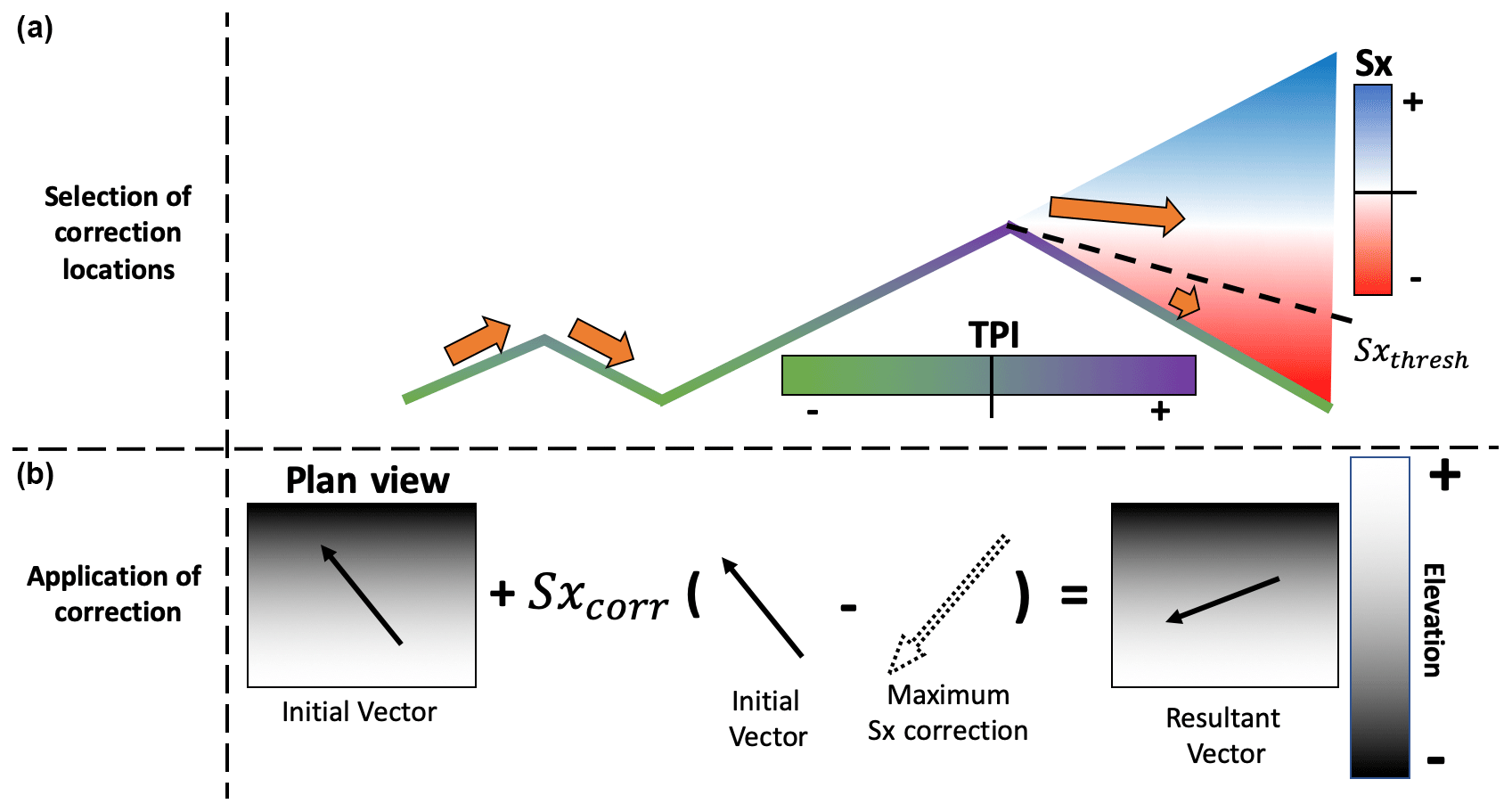
Figure 2 A conceptual outline of the Sx sheltering process. Areas where a correction should be applied are first selected, as indicated in the upper row. Only terrain elements with a positive TPI value are considered to be potential sheltering terrain elements. The smaller hill on the left has no positive TPI values along its slopes, so it does not produce an area of reduced wind speeds in the lee. The hill on the right does have a positive TPI value at its peak, so it is considered for sheltering. The Sx values in the lee side of the peak are examined and compared to the threshold Sx value, Sx_thresh, calculated in Eq. (6). Grid cells with Sx angles larger than this threshold angle experience a correction to their U and V wind speeds, as detailed in the second row of the figure. We consider the maximum deflection of the lee-side vector to be a rotation about the elevation gradient of the grid cell. This maximum correction is then applied to the initial vector with a correction factor, Sx_corr, as calculated in Eq. (7). The resultant vector is thus a mixture between the initial vector and the maximum possible correction.

2.2 Mass-conserving wind solver

After adjusting the wind field according to terrain descriptors or after ingesting any arbitrary wind field from forcing data, the resultant wind field is not guaranteed to be divergence-free. Because ICAR is an incompressible atmospheric model, this would mean a violation of mass conservation. Thus, some further correction to the 3D wind field must be applied to ensure mass conservation. In the original ICAR model, this is ensured by calculating the divergence for each model layer and prescribing the grid-relative vertical velocity at the top of each layer such that divergence is eliminated. This is sometimes referred to as the “kinematic method” of balancing the winds (O'brien, 1970; Homicz, 2002). Unfortunately, this method is known to produce excessive vertical motion even for modest amounts of residual divergence (Goodin et al., 1980). Figure 3 shows the strong vertical winds which are often observed in high-resolution simulations using the ICAR model with the kinematic method for balancing the 3D wind field. The strong vertical winds observed in the ICAR simulations are due to (a) large grid distortions in complex terrain at high resolutions, (b) the use of high-resolution forcing data from a compressible atmospheric model, and (c) the kinematic solution for vertical wind itself (Eq. 9 in G16). As the horizontal resolution is reduced, the magnitude and variations of the vertical motions are reduced. As a result, simulations with the ICAR model at coarser resolutions exhibit less strong vertical motion than shown here. However, such simulations still exhibit increasing vertical motion as a function of height due to the use of the kinematic solution for vertical velocity (O'brien, 1970). This results in excessively strong vertical motion at the model top and explains the sensitivity of ICAR to the height of the model top and choice of upper boundary condition reported in Horak et al. (2019) and Horak et al. (2021).

This issue alone motivates the implementation of a new approach to balancing the 3D wind field. When using the empirical adjustment of the 3D wind field described above, even more divergence is introduced to the wind field, resulting in entirely nonphysical vertical velocities. Clearly another technique for calculating vertical velocity is required for high-resolution applications.

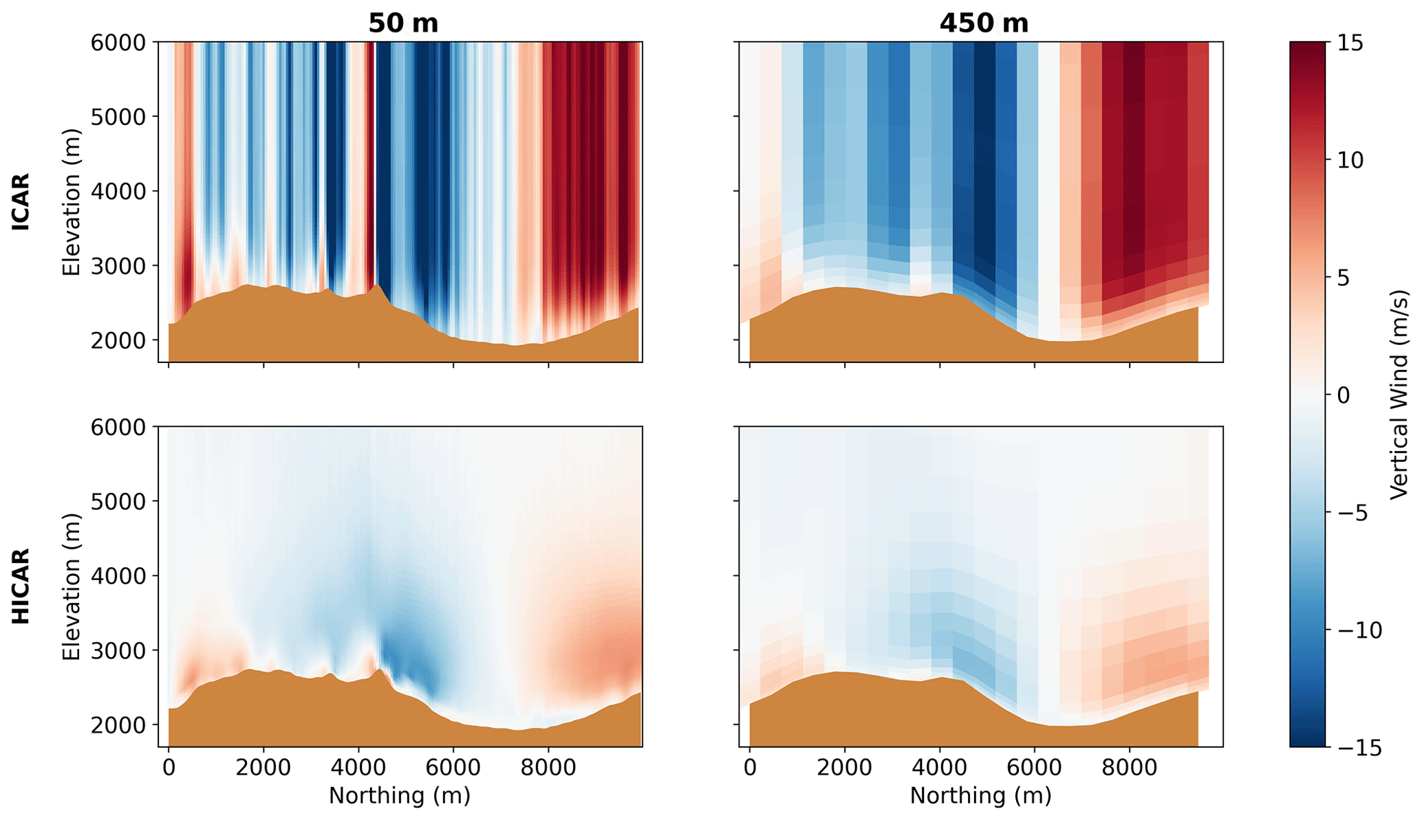
Figure 3 Comparison of vertical motion between ICAR and HICAR at 50 and 450 m resolutions for an arbitrary simulation time step. ICAR is shown in the first row, HICAR in the second.

HICAR employs a method for calculating a mass-conserving wind field which is based on a variational calculus technique. This technique has been developed over prior decades of wind modeling and pollutant transport (Sasaki, 1958; Sherman, 1978; Ross and Fox, 1991), and it has been adapted into a variety of wind models (Moussiopoulos et al., 1988; Forthofer et al., 2014). Wind tunnel experiments and field observations have routinely demonstrated the ability of this technique to simulate speed-up and deflection of flow around obstacles (Ross and Fox, 1991; Forthofer et al., 2014; Wagenbrenner et al., 2016). The method works by solving an optimization problem where two functions are reduced: the divergence of the wind field and the total deviations of the solution wind field from the initial wind field:

$$\begin{array}{}\text{(15)}& {\displaystyle }\mathrm{Div}& {\displaystyle }={\displaystyle \frac{\mathrm{d}\mathit{\rho }u}{\mathrm{d}x}}+{\displaystyle \frac{\mathrm{d}\mathit{\rho }v}{\mathrm{d}y}}+{\displaystyle \frac{\mathrm{d}\mathit{\rho }\dot{w}}{\mathrm{d}\dot{z}}},\text{(16)}& {\displaystyle }\mathrm{Diff}& {\displaystyle }=(u_{\mathrm{i}}-u{)}^{\mathrm{2}}+(v_{\mathrm{i}}-v{)}^{\mathrm{2}}+\mathit{\alpha }(w_{\mathrm{i}}-w{)}^{\mathrm{2}},\end{array}$$

where u and v refer to the eastward and northward wind speeds, w refers to the vertical wind speed, and $\dot{w}$ refers to the contravariant, grid-relative wind speed. All of the x_i variables indicate initial values. The distinction between w and $\dot{w}$ is necessary when the optimization is performed on a grid with a vertical coordinate transformation such as sigma or SLEVE coordinates (Gal-Chen and Somerville, 1975; Schär et al., 2002) and is further detailed in Ross et al. (1988). An excellent overview of the math used to solve this optimization problem and a discussion of various considerations is given in Homicz (2002), and a general review is provided by Ratto et al. (1994). Because an initial guess is required for w_i, HICAR allows the user to specify vertical motion as an input variable. Otherwise, w_i is taken to be 0 such that vertical motion is minimized. In the above equations, the variable α is used to control the relative weighting of changes to horizontal or vertical motion. This allows the solution to account for effects of atmospheric stability if one makes α a function of atmospheric stability. For example, larger values of α increase the weighting of changes to w from its initial value relative to changes of u and v from their initial values. This means that a better solution to the minimization would be found by preferring changes to u and v over w when eliminating divergence. The result of this is more deflection around terrain and less vertical motion, which one would expect during stable atmospheric conditions. A demonstration of the effects of different values of α is given in Fig. 4, showing the wind field generated by the maximum (1.0) and minimum (0.1) values that α is allowed to take. For the stable condition (α=1.0) we see surface wind speeds approaching 10 m s⁻¹ over the ridge crest and blocking of flow upwind of the ridge. Correspondingly, vertical motion is around ±2 m s⁻¹ over the ridge. For the unstable case (α=0.1), there is comparatively little deflection of the flow field upwind of the ridge and little speed-up over the ridge crest. Vertical motion is significantly enhanced in the unstable case versus the stable case. As such, α can be used to select different solutions to the optimization problem depending on atmospheric stability.

In our implementation, the α variable is calculated at each input time step and for each grid cell according to the atmospheric stability at that location according to

$$\begin{array}{}\text{(17)}& {\displaystyle }\mathit{\alpha }& {\displaystyle }=\sqrt{\mathrm{1}-\mathrm{0.5}{\displaystyle \frac{\sqrt{\mathrm{1}+\mathrm{4}F{r}^{\mathrm{4}}}-\mathrm{1}}{F{r}^{\mathrm{4}}}}}\text{(18)}& {\displaystyle }Fr& {\displaystyle }={\displaystyle \frac{\mathrm{WS}}{L\cdot N}},\end{array}$$

where Fr is the Froude number, WS is the wind speed, L is the scale length, and N is the Brunt–Väisälä frequency (BVF). Equation (17) comes from Moussiopoulos et al. (1988) and is straightforward, but the calculation of the Froude number deserves further discussion. In order to calculate α in 3D, the Froude number must also be calculated in 3D. To do this, WS, L, and N are calculated for each grid cell. The scale length, L, is the height difference between the grid cell height and the largest downwind terrain element, plus some constant to ensure a minimum value for L. L is calculated for each grid cell and each wind direction at initialization so that it can be easily looked up at runtime. Some search radius must be imposed when calculating L, which we set to 4 km. The Brunt–Väisälä frequency is then calculated by considering the column of air above the grid cell for which it is calculated. If there is a downwind obstacle, the column of air extends from the current grid cell height up to the altitude of the downwind obstacle. If there is no obstacle, the BVF is calculated using a difference over the current grid cell. The effect of these considerations is a Froude number which describes the ease of lifting a parcel of air over a given downwind obstacle. This approach of using a spatially and temporally varying α differs from prior implementations of the Sherman (1978) technique, where either α was set to 1.0 (Forthofer et al., 2014) or where α varied in time but not in space (Moussiopoulos et al., 1988). Thus, our approach can handle complex situations where flow blocking varies as a function of height such that flow may be blocked at the foot of a mountain but rise over the obstacle at higher altitudes. The computational demands of this technique are relatively small in comparison to other components of HICAR (advection, microphysics), since most of its calculations are performed once at initialization, and the solutions of Eqs. (15) and (16) are only performed when ingesting new input data instead of at every physics time step.

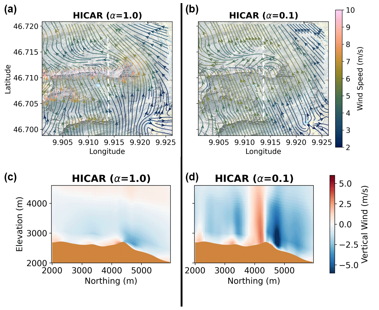
Figure 4 Demonstration of the two end-member solutions for HICAR's wind solver under the two extreme stability conditions. The plan view panels in the top row are centered on a ridge cutting horizontally across the figure. A vertical transect across this ridge is shown in (c) and (d), with the location of the transect indicated in (a) and (b) by the dotted white line. Surface wind flow lines are overlaid on a topographic base map in the upper panels, with flow line color corresponding to wind speed. The left column of the figure displays the maximum stable condition, while the right column shows the maximum unstable condition.

2.3 Advection and physics parameterizations

The original ICAR model offers a first-order upwind advection scheme. Although this scheme is highly diffusive (Schär et al., 2002), it has the advantage of low computational demand, making it suitable for ICAR's original development purposes and target resolutions. For our application at higher resolutions, and particularly with an interest in strongly heterogeneous precipitation patterns at the ridge scale, a less diffusive advection scheme was required. The issue of numerical diffusivity in complex terrain has been well documented (Westerhuis et al., 2021; Lundquist et al., 2012). Higher-order advection stencils (odd-ordered up to fifth order) have thus been implemented in the HICAR model. These schemes, in combination with the SLEVE coordinate system (Schär et al., 2002; Kruyt et al., 2022), reduce numerical diffusion in HICAR simulations. To achieve larger physics time steps, a pseudo-Runge–Kutta 3 (RK3) advection integration is added to HICAR (Wicker and Skamarock, 2002). Lastly, the use of RK3 time stepping required the addition of a monotonic flux limiter for the standard advection scheme (Wang et al., 2009).

Since the original publication of G16, numerous physics parameterizations have been added to the model and will be detailed in a future publication. It is of importance to this paper that the Noah land surface model (LSM) (Ek et al., 2003), Morrison microphysics scheme (Morrison et al., 2009), RRTMG radiation scheme (Thompson et al., 2016), and YSU PBL scheme (Hong et al., 2006) have all been added to the model and will be used for the simulations which follow in later sections.

2.4 Asynchronous I/O

As model efficiency increases, it is natural to push the model to run for larger domains and larger time periods. Additionally, as the simulation resolution increases, forcing data of a higher resolution are needed. The cumulative effect of these two points is that efficient, high-resolution models must output and input large amounts of data (Prein et al., 2015). For example, for the setup used in Sect. 4.2.1, 1 d of simulation requires reading 11 GB of forcing data and outputting 14.5 GB of data, depending on output variables selected. To avoid blocking I/O operations on the runtime loop and to facilitate a “many programs, one file” access pattern, an asynchronous I/O strategy was adopted. This is shown in Fig. 1 via the blue elements on the left. Input and output are handled by a few processes which are split from the simulation processes at initialization. These I/O processes then coordinate their file access through parallel NetCDF I/O, resulting in less demand on the file system and eliminating the need for stitching together output files in post-processing. These changes make the model faster by overlapping I/O with physics processes and make it possible to directly use simulation output to force one-way nested runs, as done in Sect. 4.2.1.

3 Model setup and datasets

3.1 COSMO model

The Consortium for Small-scale Modeling (COSMO) model is operationally run by the Swiss weather service, MeteoSwiss, over a domain encompassing Switzerland (http://www.cosmo-model.org, last access: 25 April 2023). COSMO is a nonhydrostatic, compressible atmospheric model capable of simulating the state of the atmosphere over complex terrain such as the Swiss Alps. Predicted variables from COSMO such as temperature, humidity, and wind speeds are made available by MeteoSwiss. Output from the 1.1 and 2 km resolution COSMO simulations, COSMO1 and COSMO2, respectively, are used in this study. COSMO2 output is used to force the 1350 m WRF, ICAR, and HICAR simulations discussed in Sect. 4.1 and 4.2.1, while COSMO1 output is used to force the 250 m HICAR simulation in Sect. 4.2.2 and 4.3, as well as the 450 m HICAR simulation in Sect. 4.4. The HICAR simulations are forced with specific humidity, temperature, pressure, and the 3D wind field (U, V, W) from the COSMO model. All COSMO variables are bilinearly interpolated in 3D to the HICAR grid using latitude, longitude, and vertical height. Then, specific humidity and temperature are forced at the boundaries, while pressure and winds are input for the full 3D grid, with the winds being further modified using the downscaling scheme described in Sect. 2.

3.2 WRF model

The Weather Research and Forecasting (WRF) model (Skamarock et al., 2008) is a nonhydrostatic and compressible atmospheric model used widely in research and operational forecasting (Benjamin et al., 2016). WRF has also been successfully run at very high resolutions (50 m) over the complex terrain of the Alps (Gerber et al., 2018, 2019; Goger et al., 2022; Kruyt et al., 2022). For these reasons, we use WRF in this study to demonstrate a “gold standard” for atmospheric modeling in comparison to HICAR runs. All output from the WRF model comes from prior simulations first presented in Gerber et al. (2018) and thus guided the choice of spatiotemporal domain for some of the simulations presented in Sect. 4. All WRF data presented are at a 50 m horizontal resolution.

3.3 ICAR and HICAR setup

Simulations using the ICAR and HICAR models, introduced in Sect. 2, are presented in Sect. 4. The HICAR simulations utilize the YSU PBL scheme, Noah land surface model, RRTMG radiation scheme, and Morrison two-moment microphysics scheme. The surface scheme implemented follows that detailed in Chen and Dudhia (2001). The Morrison microphysics scheme was chosen due to its demonstrated efficacy in forecasting precipitation in complex terrain (Liu et al., 2011) and use in the WRF simulations of Gerber et al. (2018). Only the wind fields from the ICAR simulations are analyzed, and because there is no physics–dynamics coupling in either ICAR or HICAR, ICAR was not run with these physics parameterizations enabled.

HICAR has been developed as a variant of the ICAR model, as these models share a core code base. The HICAR variant of ICAR can be turned on by passing “HICAR” to the variant option of the namelist file. This switches on a number of namelist options, ensuring that the configuration is optimized for high-resolution runs in complex terrains. Specifically, the namelist options which designate a run with the HICAR model include terrain-following SLEVE coordinates, a variational-calculus-based wind solver, and wind modifications based on terrain descriptors.

3.4 Spatiotemporal domains

Section 4.1 and 4.2.1, as well as the figures presented in Sect. 2, use the same 50 m domain introduced in Gerber et al. (2018). It is roughly 10 km × 10 km, with the 50 m horizontal resolution simulations covering a 24 h period over the day of 5 March 2016. This domain covers the upper Dischma Valley outside Davos, Switzerland. We adopt the terminology “xx m simulation” to refer to the horizontal resolution of a simulation. The 50 m HICAR and ICAR simulations for this run are nested within 150, 450, and 1350 m simulations of the same respective model, following the methodology of Gerber et al. (2018) for their WRF runs. Importantly, ICAR–HICAR allows the use of a coarser vertical grid than WRF (Horak et al., 2021). As a result, the WRF simulations use 40, 40, 60, and 90 vertical levels for the 1350, 450, 150, and 50 m simulations, while ICAR–HICAR used only 20, 20, 60, and 60.

Section 4.2.2 and 4.3 discuss results from a 250 m simulation of HICAR covering most of the Swiss Alps from Lausanne in the west to Val Müstair in the east for a roughly 280 km × 170 km domain. The simulation was run for the month of January 2017.

Section 4.4 repeats a benchmarking setup from Kruyt et al. (2022), running the HICAR model at a 50 m resolution for 5 d in March 2019 over a roughly 7.5 km × 7.5 km domain. This 50 m domain is nested within a 450 m domain, following the methodology of Kruyt et al. (2022).

High-resolution domain data for all simulations come from Gerber and Lehning (2021), which provides ASTER Global Digital Elevation Model V002 and Corine land use data at a resolution of 1 arcsec (METI/NASA, 2009; European Environmental Agency, 2006). For the HICAR simulations, these terrain data were then upscaled to the desired target resolution with no smoothing applied. In order to run the WRF model at resolutions approaching 50 m, certain considerations must be applied to the model topography. For the WRF simulations, to ensure model stability at reasonably long time steps, the terrain for all high-resolution simulations is smoothed using a 1–2–1 smoothing filter with 14 passes, and the terrain near the boundaries of the outermost domain is smoothed to match the COSMO topography. Although this smoothing procedure is not required to run ICAR and HICAR, the same smoothed terrain data as the WRF simulation are used for one HICAR simulation presented in Sect. 4.2.1. This is done in order to enable a direct comparison between WRF and HICAR for the same topography. In a future publication, potential improvements of using unsmoothed topography on wind speeds in HICAR will be examined.

3.5 Gridded datasets

In Sect. 4.2.2, two gridded datasets for precipitation are used, MeteoSwiss's RhiresD product (MeteoCH, 2013) and the precipitation product produced by the SLF Operational Snow Hydrology Service (OSHD) using an optimal interpolation (OI) technique (Magnusson et al., 2014; Mott et al., 2023). RhiresD is constructed by taking precipitation data from a dense network of precipitation gauges distributed throughout the Alps and then applying a climatological precipitation–elevation gradient to extrapolate observations beyond gauges using a version of the PRISM algorithm (Daly et al., 1994). The OSHD precipitation product is obtained by first partitioning RhiresD into solid and liquid precipitation and then updating the snowfall fraction by assimilating snow station data from 350 locations using optimal interpolation (Magnusson et al., 2014). This allows for a higher station density at higher elevations relative to RhiresD and minimizes underestimates of precipitation during snowfall events due to gauge undercatch. Of course, selecting for snow station sites introduces other spatial biases in station representativeness (Grünewald and Lehning, 2015). A full description of the OI procedure used in the OSHD product can be found in Mott et al. (2023).

(Shin and Hong, 2015)(Hong and Pan, 1996)

Table 1 Model configurations. For advection order, the number preceding H refers to the numeric order of the horizontal advection stencil and the number preceding V to that of the vertical. n/a – not applicable

4 Model demonstrations

4.1 Wind fields

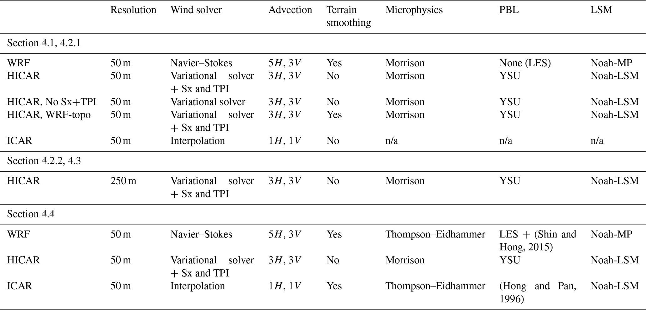
In Sect. 2.2, the effects of the changes to the wind solver were shown for comparison with ICAR (Fig. 3) and for a demonstration of their ability to simulate atmospheric stability (Fig. 4). To discuss the wind solver of HICAR in the context of existing atmospheric models, we present results comparing HICAR to the WRF model. Figure 5 shows a plan view of multiple model simulations at 50 m over complex terrain in the upper Dischma Valley of Davos, Switzerland. As discussed in Sect. 2, the COSMO forcing data provided are expected to capture the effects of mountain waves which the linear wind solver of ICAR is designed to capture, so this module of ICAR was turned off. As a result, the ICAR simulation shown is composed of bilinearly interpolated COSMO2 data. The surface flow field from ICAR is quite homogenous as a result, with uniform southwesterly flow over the domain and a narrow range of wind speeds over the domain. This is in contrast to the WRF simulation, which reports various modifications to the flow pattern (blocking, cross-slope flow, terrain-induced speed-up), as well as a larger range of wind speeds. This result is instructive in that ICAR alone is not suitable for high-resolution simulations. WRF also reports higher wind speeds at ridge crests than any of the HICAR simulations, but WRF has been found to overestimate speed-up of winds over topography (Gerber et al., 2018; Gómez-Navarro et al., 2015; Goger et al., 2022; Umek et al., 2021).

For examining the effects of the wind solver detailed above, we present two HICAR simulations: one with the empirical adjustments based on terrain descriptors and one without. The simulation without terrain descriptors uses a procedure to diagnose its winds which is similar to that employed by models like WindNinja (Forthofer et al., 2014) but with the distinction of using a spatiotemporally varying value for α (Eq. 17). This simulation already captures a wider range of surface wind speeds than the base ICAR model and offers some of the flow field deflection observed with the WRF model. This is consistent with prior studies which have employed the technique from Sherman (1978). Once the terrain descriptors are used, we see that certain features of the flow field present in the WRF simulation also emerge in the full HICAR run. Of note are the cross-slope flows and lee-side reductions in wind speed. Due to the improved terrain representation possible with the ICAR and HICAR models, these flow features develop for secondary valleys not fully resolved in the WRF topography. This demonstrates the added value of this two-step approach to generating a diagnostic, mass-conserving wind field.

The advantages of the terrain descriptors are shown in Fig. 6 as well. This figure presents a vertical cross section of modeled flow across the Sattelhorn ridge, which is in the upper center of Fig. 5. The WRF model shows a large eddy on the lee side of the ridge, with a long horizontal extent and reduced wind speeds relative to the flow outside the lee. This eddy also gives rise to up-slope flow at the surface of the lee of the ridge. The HICAR run simulates a similar dynamic structure. The eddy present in HICAR has a shorter horizontal extent and is stronger, resulting in higher wind speeds within the eddy and faster reverse flow at the surface of the lee. Despite these differences in the properties of the eddy, the ability of HICAR to predict the presence of such flow features is a surprising result, since no prior applications of the Sherman (1978) technique have reported such behavior. We attribute this to our use of terrain descriptors, which predispose the solution of Sherman (1978) to generate an eddy in the lee, all of which may be due to the sharper terrain represented by HICAR. It is easy to imagine how this approach of preconditioning a wind field and then using a diagnostic, mass-conserving solver could be used to parameterize other dynamic effects and has previously been shown to yield reasonable results when parameterizing thermally driven winds (Forthofer, 2007). We also note that the calculation of the terrain-descriptor-based corrections depends upon somewhat arbitrary constants and could thus be adjusted to yield eddies of varying horizontal extent. This tuning of the terrain-descriptor-based adjustments will be done in a future study using distributed observations of winds in complex terrain as a basis for tuning and validation.

The differences in terrain representation between WRF and ICAR–HICAR are also displayed in Figs. 5 and 6. WRF and other models which prognostically solve for winds rely on spatial gradients of pressure to calculate wind speeds. In order to simplify the lower boundary condition, these models also typically employ terrain-following coordinates where model coordinate surfaces slope as the terrain does. This means that high-resolution simulations will feature large coordinate distortion, and pressure differences in the horizontal may become quite large as one vertical cell surface exists at lower elevations than another. This may lead to large pressure gradients which require very fine time steps to stably integrate. The model terrain is typically smoothed to allow for smaller grid distortions, smaller pressure gradients, and thus larger time steps. Recent implementation of an immersed boundary method in WRF allows this entire consideration to be skipped, although such a domain discretization comes with its own trade-offs (Lundquist et al., 2012).

The above discussion is valid for atmospheric models which solve prognostic equations for momentum. Neither the ICAR model nor the HICAR variant do this, opting for diagnostic solutions for the wind field instead. As a result, issues of model stability arising from terrain steepness do not exist, and we can include model terrain without any artificial smoothing or implicit numerical diffusion. This is apparent in the elevation profile in Fig. 6 and, to a lesser extent, in the DEM in Fig. 5. The difference in terrain used may lead to the different lee-side dynamics when comparing the HICAR and WRF simulations. This ability of ICAR and HICAR to represent the terrain without any artificial smoothing is a major strength of both models. High-resolution atmospheric modeling is assumed to yield more accurate forecasts, in part through improved representation of the underlying terrain. If HICAR can represent topography more accurately than WRF at the same horizontal resolution and without explicit numerical diffusion, it allows for model resolutions effectively higher than WRF.

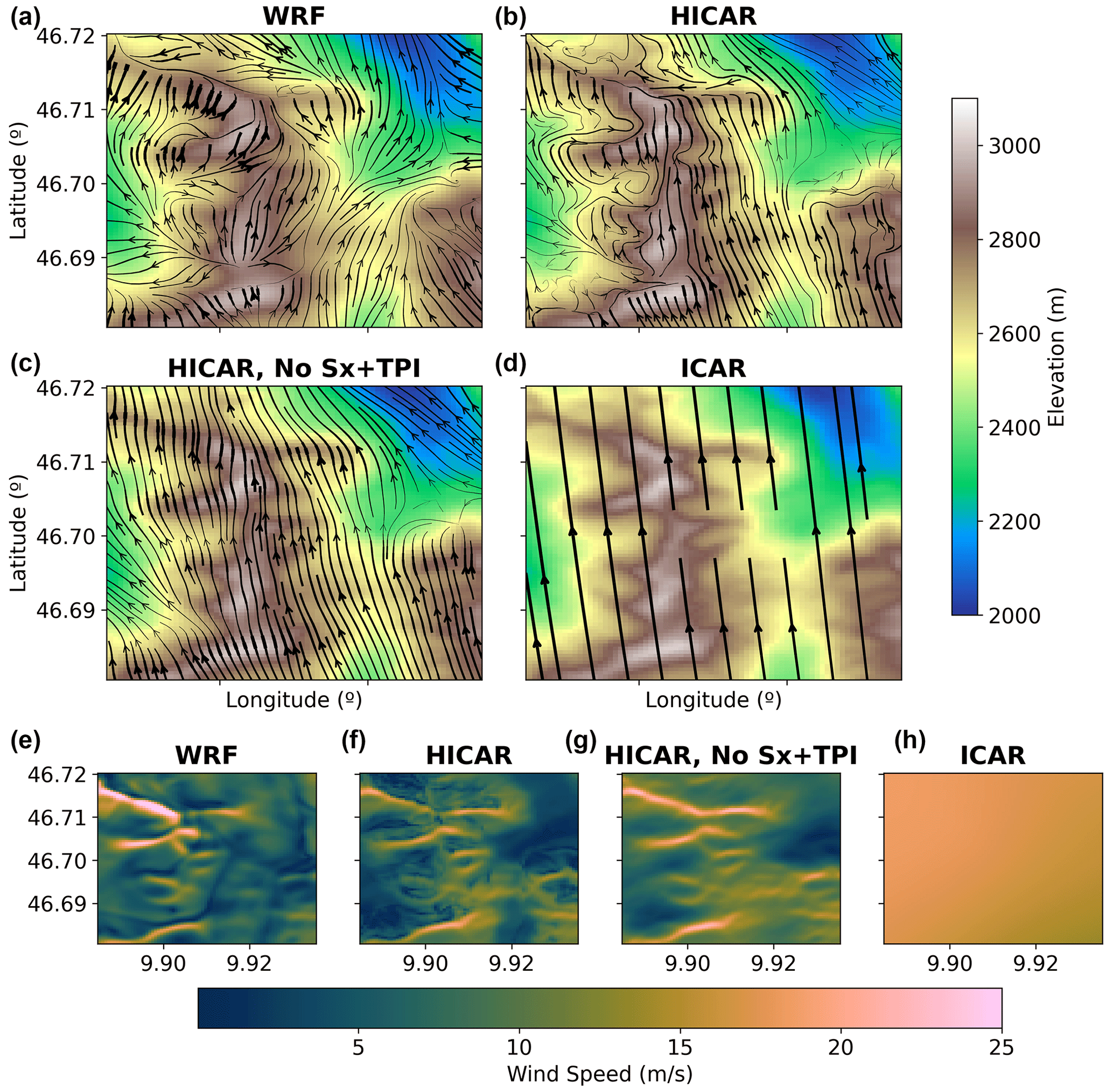
Figure 5 Comparison of surface flow fields at a 50 m resolution between models and model setups for 5 March 2016 at 00:00 UTC+1. The upper four panels show flow fields overlaid on model topography. Model topography is smoothed for the WRF run compared to the HICAR and ICAR runs. Thickness of flow lines corresponds to wind speed, with thicker flow lines indicating higher wind speeds. The lower row of panels displays the surface wind speeds of the various model runs. The sparser flow lines for the ICAR simulation are a plotting decision to avoid redundancy and do not reflect a difference in the simulation setup. The orange arrow indicates the location of the Sattelhorn ridge, which is shown in profile in Fig. 6.

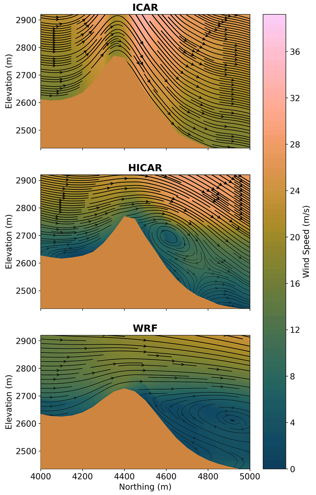
Figure 6 Profile view of flow fields at a 50 m resolution between models for 5 March 2016 at 02:00 UTC+1. Wind direction is indicated by the flow lines, and line thickness corresponds to wind speed, where thicker lines show higher wind speeds. Wind speed is given by the background color. A profile of the underlying terrain is shown in each panel, with the WRF simulation having smoother terrain than the ICAR or HICAR simulations.

4.2 Precipitation distribution

4.2.1 Ridge scale

The above discussion of terrain representation also plays an important role in precipitation distribution, as displayed in Fig. 7. There are noticeable differences in the snowfall transects of the two HICAR simulations, one using the unsmoothed topography (HICAR) and the other using WRF's smoothed topography (HICAR, WRF-topo). This result supports the above point that HICAR's improved terrain representation leads to a higher effective model resolution, impacting the simulation results. We also note a strong wet bias over the domain for the WRF model, with precipitation amounts nearly double what was recorded at a snow depth station located in the domain (Fig. 7). This wet bias was attributed to excessive orographically enhanced precipitation in Gerber et al. (2018). The snowfall transects reveal ridge-scale differences in precipitation for all model simulations, with the windward (left) side of the ridge receiving approximately 15 % more snowfall than the leeward (right) side in the HICAR simulations. The WRF simulation shows a similar although more modest ridge-scale difference, with a positive snowfall anomaly (relative to the mean over the transect) beginning on the windward side and continuing until just downwind of the ridge, followed by a steady decrease in snowfall anomaly. The main difference between the HICAR and WRF simulations is the magnitude of the windward and leeward differences. This can be partly explained by the lee-side dynamics simulated by both models. Taking the flow profiles shown in Fig. 6 to be representative of the flow differences over the 24 h event, we note that HICAR has higher wind speeds aloft on the lee side of the ridge due to the presence of the eddy. The peak in precipitation on the windward side is likely due to blocking of the low-level flow and reduced wind speeds on this side of the peak (Fig. 6). We note a positive anomaly in snow depth just downwind of the ridge, which we attribute to the strong horizontal wind speeds aloft, in line with previous studies of preferential deposition (Mott et al., 2014; Wang and Huang, 2017). In fact, the HICAR snow depth distributions show a similar windward and leeward pattern to results obtained by Comola et al. (2019) using an LES model over ideal topography. This cumulative effect of the flow field on snow depth can be realized intuitively by tracing the flow lines of Fig. 6 across the ridge and imagining snow sedimentation given a constant sedimentation rate. The question of whether this flow pattern is accurate for this particular event has not been demonstrated, but given the proven accuracy of the HICAR advection scheme (Wang et al., 2009), the resultant deposition pattern is certainly physically consistent with the given flow field. This discussion demonstrates the research utility of HICAR: it can be used to efficiently (Sect. 4.4) test different flow patterns at the ridge scale and see how they affect particle–flow interactions. A later validation of HICAR flow fields would determine how predictive the simulated deposition patterns are.

Figure 7 Differences in snowfall over the upper Dischma Valley for a 24 h snowfall event on 5 March 2016. All terrain data displayed are from the unsmoothed HICAR run. All values of snowfall are reported in centimeters, with the WRF and HICAR snowfall values converted from mass to depth assuming a constant density of 100 kg m⁻³. Panel (a) shows a DEM of the area, with a dot in the valley indicating the location of a snow depth sensor and an arrow indicating the location and direction (left–right) of the transect shown in the upper right panel. This arrow points along the prevailing wind direction during the 24 h snowfall. Panel (b) shows snow depth transects across the Sattelhorn ridge for three model simulations: WRF, HICAR, and HICAR run with the same smoothed topography as WRF. Mean snowfall is almost twice as large in WRF as in HICAR, so snow depth is reported as a percentage of the mean snow depth along the transect in order to compare the HICAR and WRF simulations on the same graph. Panels (c) and (d) show the spatial distribution of snow depth across the domain, with the value recorded at the snow depth station over the 24 h period (20.3 cm) overlaid.

4.2.2 Range scale

Accurate high-resolution precipitation estimates in complex terrain are a slippery target (Lundquist et al., 2019; Bonekamp et al., 2018). Gauge-based gridded products are subject to gauge undercatch and assumptions about the spatial patterns used to interpolate them (Rasmussen et al., 2012; Collados-Lara et al., 2018; Lundquist et al., 2010). Radar products meanwhile suffer from occlusion when scanning in complex terrain (Germann et al., 2022). As a result, high-resolution comparisons of modeled versus observed precipitation in complex terrain deserve careful consideration to offer any form of model validation. We spare any detailed quantitative validation for a future study and instead offer a comparison of different gridded precipitation products for the sake of discussion.

Figure 8 shows accumulated precipitation for January 2017 from two gridded products and a 250 m HICAR simulation. We first note that the majority of storms during January 2017 came from the northwest, and our simulation domain for HICAR extended slightly beyond the boundaries of the figure shown to just include the Swiss Plateau. The HICAR simulation is forced with only water vapor from COSMO1, so the microphysics require some time to “spin up”, generating hydrometeors and thus precipitation. This may explain some of the lower precipitation amounts along the pre-Alps in the upper northwest of the figure relative to both RhiresD and the OSHD precipitation product.

Overall, Fig. 8 shows remarkable agreement between HICAR and the two gridded precipitation products for a 1-month winter period. The OSHD precipitation product gives larger precipitation values at higher elevations than RhiresD since it is generated by back-calculating precipitation from snow water equivalent, avoiding gauge undercatch during snowfall events (Magnusson et al., 2014). This result suggests that the larger precipitation values obtained from the HICAR simulation are possible. The inter-alpine areas (center) of the domain, however, show less precipitation in HICAR than either gridded product, especially in the valleys. However, these differences between HICAR and the other gridded products are comparable to differences observed between the gridded products themselves. Lastly, we note that the product using climatological averages for its interpolation, RhiresD, returns a smoother field of precipitation than either HICAR or the OSHD product. The OSHD product yields stronger elevation gradients of precipitation, which is likely due to its higher station density at higher elevations relative to RhiresD and its ability to capture unbiased precipitation during snowfall events. This suggests that the stronger gradients observed from HICAR are appropriate. None of this discussion is to assert the accuracy of one product over another, but is instead to demonstrate that HICAR's precipitation estimate is as consistent with existing precipitation products as those products are with each other.

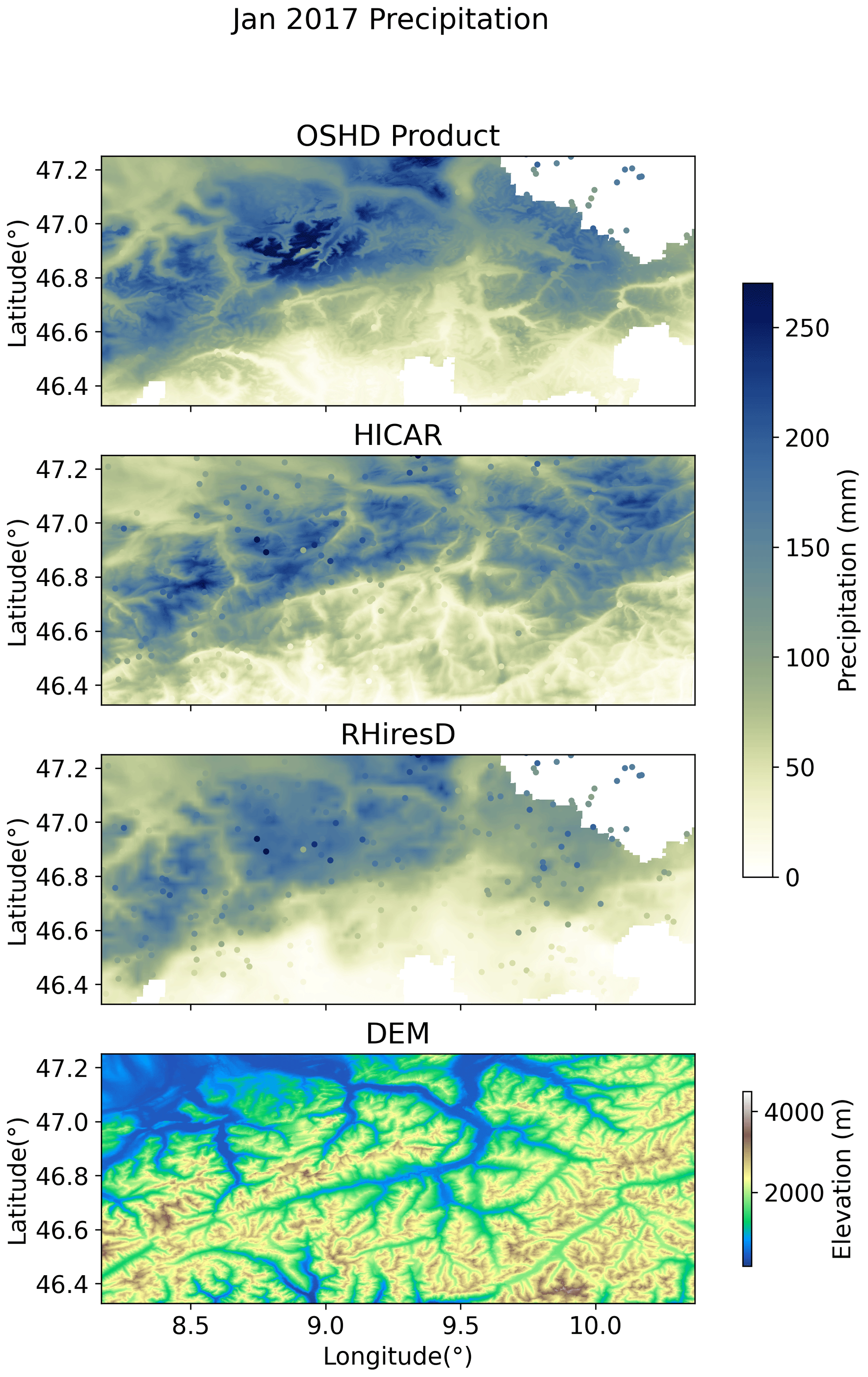
Figure 8 Precipitation over the central and eastern Swiss Alps during January 2017 at a 250 m resolution. All three plots of precipitation have point data from the OSHD product overlaid as dots. Since these mostly coincide with the same values for the OSHD product, the dots are often indistinguishable from the background field in the top panel.

4.3 Cold air pooling

Figure 9 shows a cold air pooling event on the morning of 24 January 2017. We observe that, over the course of the early morning hours, strong mesoscale winds recede from over the valley, allowing a cool, stable boundary layer to develop and for that cool air to migrate toward lower elevations. This surface layer is ultimately remixed as wind speeds increase and surface cooling decreases around 09:00 local time. These results are somewhat surprising, as a parameterization of thermally driven flows is not yet included in HICAR. Thus, the flow patterns shown are largely unaware of the evolving thermal stratification of the valley. However, the wind solver used in HICAR is designed to minimize differences between its wind field and the wind field supplied from the forcing data. The driving model, in this case COSMO1, has been shown to simulate valley winds supportive of cold air pooling (Goger et al., 2018), so if the LSM of HICAR simulates a cooling of the surface, cold air pooling as shown in Fig. 9 is possible. This figure demonstrates an important caveat of the HICAR model: its dependency on physically consistent winds from forcing data. The simulation shown here was forced with COSMO1 data at the boundaries, while the model runs in prior sections examining HICAR's wind field were forced with COSMO2 data. A test of HICAR's sensitivity to the resolution of the driving model is needed but is beyond the scope of this study. At present, only forcing data at resolutions where mountain waves can be expected to be resolved have been used. Yet, as noted in Sect. 2, regional forecasting offices are increasingly providing model output at these resolutions.

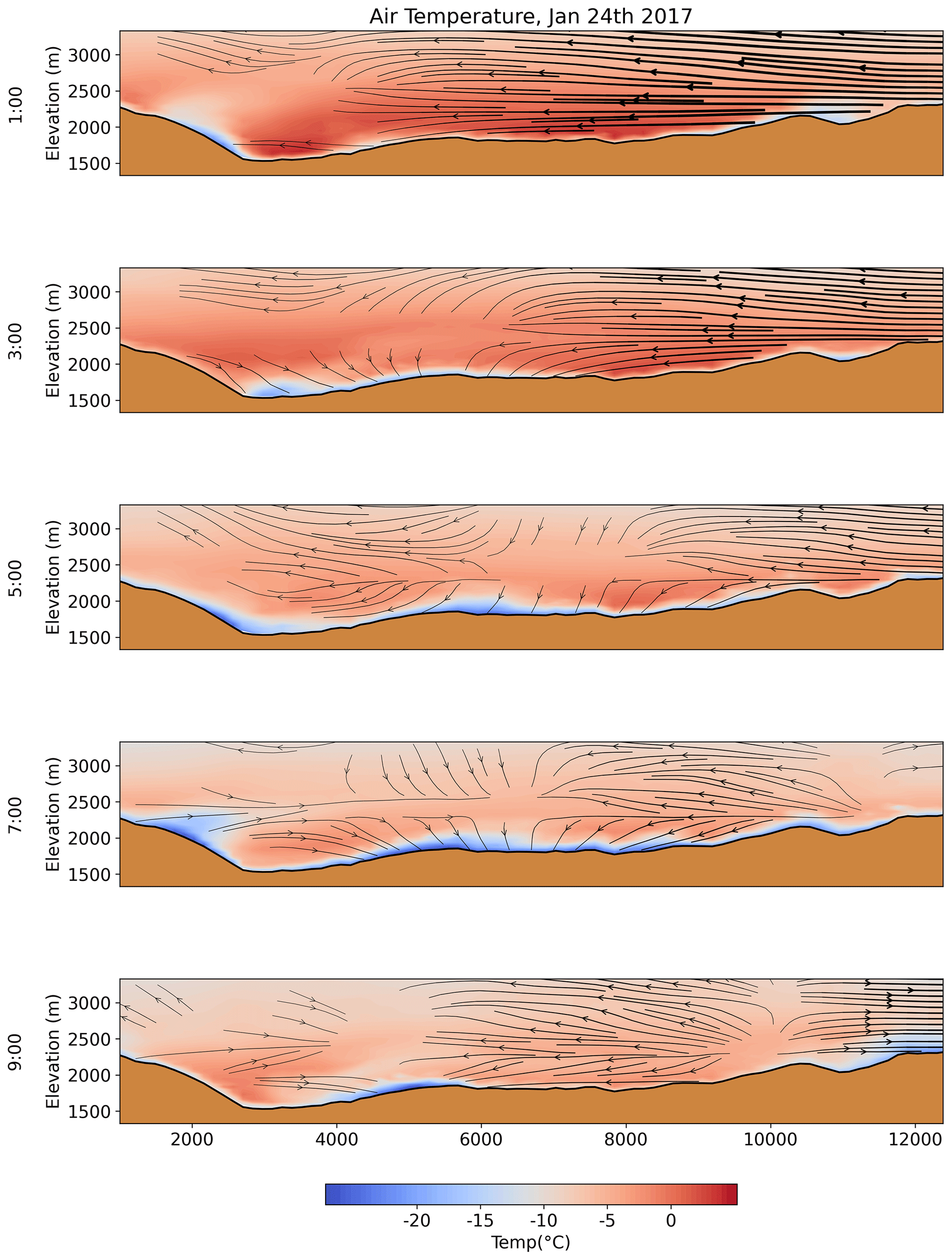
Figure 9 The development and diffusion of surface cooling for an alpine valley during dawn. The plot shows a small area of the 250 m Swiss Alp domain introduced in Sect. 3.4. The local time is indicated on the y-axis label. Wind vectors are plotted for wind directions along the transect. Thicker vectors indicate higher wind speeds, and winds below 0.2 m s⁻¹ are not plotted.

4.4 Computational efficiency

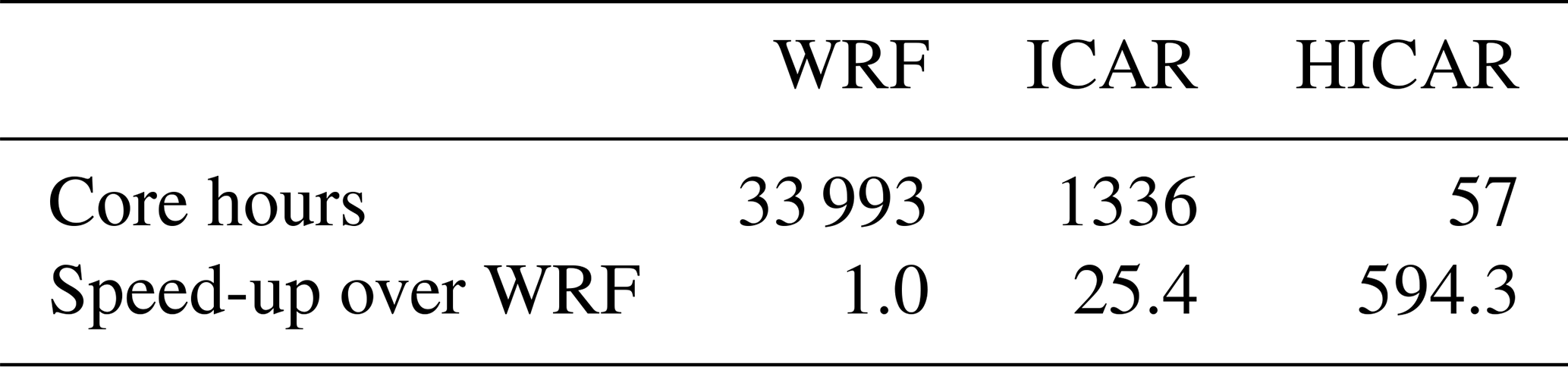
The main reason why HICAR may be attractive as a model is its computational efficiency relative to existing atmospheric models such as WRF and COSMO. Aside from HICAR's improved representation of terrain, the model is not expected to simulate physical phenomena better than more complex models. Thus, understanding its computational demand is central to establishing its utility. To quantify this demand, we repeat a benchmarking setup described in Kruyt et al. (2022). We run HICAR at a 50 m resolution over a roughly 7.5×7.5 km domain for a 5 d period in March 2019, which includes several winter storms. The model numerics and physics setup is the same as those used for the above subsections for which results are shown. The results of the benchmarking test are presented in Table 1, alongside the results previously published in Kruyt et al. (2022). The main takeaway from this comparison is that HICAR uses 594 times fewer computational resources than WRF for the same simulation. Stated otherwise, a year of simulation over this domain with WRF would require a significant allotment of computing time (∼ 350 000 node hours, assuming 36 cores per node). With HICAR, the same simulation represents a fraction of a modest project allocation (∼ 590 node hours).

The more than 20-fold speed-up of HICAR relative to ICAR is also somewhat surprising. This result is best explained by the switch from the GNU Fortran compiler to the Cray compiler and aggressive optimization of the model code outside of the physics parameterizations. Of these optimizations, one of the most effective at reducing runtimes was moving to batched message passing between parallel processes. Testing of Coarray Fortran, on which ICAR is parallelized (Rasmussen et al., 2018), has revealed the Cray compiler to have a faster implementation of this Fortran standard than GNU. Additionally, the high-performance computing architecture used in this study is the Piz Daint computer, featuring Cray XC40 compute nodes. The use of a native compiler may contribute to speed-up as well. The WRF runs here were performed with the Intel compiler and were not rerun for this study with the Cray compiler due to constraints on computational resources. Prior studies using WRF on the same computing architecture additionally recommend the use of the Intel compiler (Gerber and Sharma, 2018).

Table 2 Core hours per simulation day for benchmarking run.

5 Conclusions

In this paper we have introduced the high-resolution variant of the ICAR model, HICAR. We detailed its primary modifications to adapt it for simulations over high-resolution complex terrain. This consists primarily of a new approach to solving for a 3D wind field which utilizes terrain descriptors, TPI and Sx, to precondition the input wind field to approximate some expected effects of the topography on the flow field (Figure 2). These effects are parameterized simply and rely on assumptions and somewhat arbitrary constants. The model's sensitivity to these constants will be further investigated in a future study. After this correction step, the preconditioned wind field is fed into an optimization routine, which makes the resulting field mass-conserving while minimizing changes to the preconditioned field (Fig. 1). A novel approach to the diagnostic wind solver is adopted which allows atmospheric stability to influence the solution as it varies in time as well as space. This allows low-level flow blocking, lee-side recirculation, and cross-slope flows to be simulated by the model. These changes to the wind solver, in addition to a new advection scheme and physics parameterizations, enable the results demonstrated in Sect. 4.

We observe a marked improvement in the representation of wind fields in complex terrain over the base ICAR model when comparing against the WRF atmospheric model (Fig. 5). By avoiding the Navier–Stokes equations, HICAR is also able to run stably over steeper terrain than WRF and may thus resolve flow features induced by small-scale topography which WRF cannot (Fig. 5). These improvements to the wind field make HICAR capable of simulating heterogenous snow deposition patterns in complex terrain, which show clear signals resulting from terrain–flow interactions (Figs. 6 and 7). At larger scales, precipitation patterns in complex terrain are represented to the same goodness as existing gridded precipitation products (Fig. 9). ICAR–HICAR also forgoes any consideration of pressure gradients in its dynamics, allowing it to be run without any smoothing of the underlying terrain. Most importantly, all of these developments were done while maintaining the orders-of-magnitude speed-up over WRF which ICAR originally demonstrated. The result is a model which is 594 times faster than WRF and can run at very high resolutions (50 m), extending intermediate-complexity atmospheric modeling into the resolutions typically used by land surface modelers. HICAR's ability to handle very steep terrain, coupled with its computational speed, seems well suited for modeling efforts over High-Mountain Asia, where testing of various model configurations is already performed with more computationally expensive models (Bonekamp et al., 2018). HICAR's computational efficiency also enables high-resolution simulations over long timescales, supporting climate impact studies at the regional scale and seasonal studies of coupled glacier–atmosphere or snow–atmosphere models at hectometer scales. This last point will be expanded upon in future publications, where HICAR will be coupled with an intermediate-complexity snow model to enable high-resolution forecasting of winter snowpack and spring melt. This will involve the addition of a thermal wind parameterization to improve surface flows over glaciers and snow (Mott et al., 2020), with the goal of better resolving advective surface–atmosphere processes such as turbulent heat exchange. As atmospheric models begin to regularly probe higher resolutions, HICAR enables rapid testing and iteration of various model configurations with relatively little computational cost. This makes HICAR a powerful companion to conventional atmospheric models.