Cross-evaluating WRF-Chem v4.1.2, TROPOMI, APEX, and in situ NO₂ measurements over Antwerp, Belgium

The Weather Research and Forecasting model coupled with Chemistry (WRF-Chem) is employed as an intercomparison tool for validating TROPOspheric Monitoring Instrument (TROPOMI) satellite NO₂ retrievals against high-resolution Airborne Prism EXperiment (APEX) remote sensing observations performed in June 2019 in the region of Antwerp, a major hotspot of NO₂ pollution in Europe. The model is first evaluated using meteorological and chemical observations in this area. Sensitivity simulations varying the model planetary layer boundary (PBL) parameterization were conducted for a 3 d period in June 2019, indicating a generally good performance of most parameterizations against meteorological data (namely ceilometer, surface meteorology, and balloon measurements), except for a moderate overestimation (∼ 1 m s⁻¹) of near-surface wind speed. On average, all but one of the PBL schemes reproduce the surface NO₂ measurements at stations of the Belgian Interregional Environmental Agency fairly well, although surface NO₂ is generally underestimated during the day (between −4.3 % and −25.1 % on average) and overestimated at night (8.2 %–77.3 %). This discrepancy in the diurnal evolution arises despite (1) implementing a detailed representation of the diurnal cycle of emissions (Crippa et al., 2020) and (2) correcting the modeled concentrations to account for measurement interferences due to NO_y reservoir species, which increases NO₂ concentrations by about 20 % during the day. The model is further evaluated by comparing a 15 d simulation with surface NO₂, NO, CO, and O₃ data in the Antwerp region. The modeled daytime NO₂ concentrations are more negatively biased during weekdays than during weekends, indicating a misrepresentation of the weekly temporal profile applied to the emissions obtained from Crippa et al. (2020). Using a mass balance approach, we determined a new weekly profile of NO_x emissions, leading to a homogenization of the relative bias among the different weekdays. The ratio of weekend to weekday emissions is significantly lower in this updated profile (0.6) than in the profile based on Crippa et al. (2020; 0.84).

Comparisons with remote sensing observations generally show a good reproduction of the spatial patterns of NO₂ columns by the model. The model underestimated both APEX (by ca. −37 %) and TROPOMI columns (ca. −25 %) on 27 June, whereas no significant bias is found on 29 June. The two datasets are intercompared by using the model as an intermediate platform to account for differences in vertical sensitivity through the application of averaging kernels. The derived bias of TROPOMI v1.3.1 NO₂ with respect to APEX is about −10 % for columns between (6–12) × 10¹⁵ molec. cm⁻². The obtained bias for TROPOMI v1.3.1 increases with the NO₂ column, following $C_{\mathrm{APEX}}=\mathrm{1.217}{C}_{\mathrm{v}\mathrm{1.3}}-\mathrm{0.783}$ × 10¹⁵ molec. cm⁻², in line with previous validation campaigns. The bias is slightly lower for the reprocessed TROPOMI v2.3.1, with $C_{\mathrm{APEX}}=\mathrm{1.055}{C}_{\mathrm{PAL}}-\mathrm{0.437}$ × 10¹⁵ molec. cm⁻² (PAL).

Finally, a mass balance approach was used to perform a crude inversion of NO_x emissions based on 15 d averaged TROPOMI columns. The emission correction is conducted only in regions with high columns and high sensitivity to emission changes in order to minimize the errors due to wind transport. The results suggest that emissions increase over Brussels–Antwerp (+20 %), the Ruhr Valley (13 %), and especially Paris (+39 %), and emissions decrease above a cluster of power plants in western Germany.

1 Introduction

Nitrogen oxide (NO_x= NO + NO₂) pollution is a growing concern in populated, urban areas due to its adverse effects on human health, ecosystems, and the role it plays in further atmospheric processes. In Europe, NO_x pollution sources are largely anthropogenic. Road and non-road transport account for almost half of the total emissions in Europe, while the rest are due to the energy sector (26 %), industrial processes (14 %), and small contributions from the residential sector (9 %) and agriculture (7 %; Crippa et al., 2018). High NO_x emissions have been linked to premature deaths (Jonson et al., 2017). Environmentally, NO_x pollution can lead to the eutrophication of bodies of water, particularly in regions close to emission sources (Stipa et al., 2007). Nitrogen oxides are photochemical precursors of tropospheric ozone (Sillman et al., 1990), which acts as a greenhouse gas with its own environmental and human health impacts (Lelieveld et al., 2015). Ozone production depends equally on the concentration of volatile organic compound (VOC) species and NO_x (Kleinman, 1994). Thus, the development of accurate and detailed techniques to elucidate the causes of NO_x pollution and predict its consequences is needed to put forward mitigation plans aiming to minimize detrimental effects in the future.

Spaceborne retrievals provide global distributions of key pollutants which cannot be obtained from the sparser, ground-based air quality networks. Spaceborne measurements of reactive tropospheric pollutants in the ultraviolet visible range have been in place since the 1990s, with the Global Ozone Monitoring Experiment (GOME) being launched in 1995 (Burrows et al., 1999), and its successors, the SCanning Imaging Absorption spectroMeter for Atmospheric CHartographY (SCIAMACHY; Bovensmann et al., 1999) and Ozone Monitoring Instrument (OMI; Levelt et al., 2006; Boersma et al., 2007), were launched in the mid-2000s. Each instrument was developed based on its predecessor, mainly in terms of the spatial resolution (nominally 40 × 320, 30 × 60, and 13 × 24 km², respectively) at which columns were measured. The TROPOspheric Monitoring Instrument (TROPOMI) aboard the European Space Agency (ESA) Sentinel-5 Precursor (S5P) satellite was developed to capture daily information at even higher resolution, i.e., 3.5 × 7 km² at its launch, which has improved to 3.5 × 5.5 km² since August 2019 (Veefkind et al., 2012). Due to the short lifetime of NO_x, higher-resolution monitoring is critical to capture the spatial and temporal variability in plumes, especially near urban and industrial regions with strong emission sources. Nevertheless, satellite retrievals have their limitations and uncertainties, as the observed signal depends on light absorption and scattering over a complex light path affected by clouds, aerosols, and the surface properties and the vertical profile shape of the target gas, all of which are imperfectly characterized. Thus, satellite measurements must be evaluated against independent data to determine their uncertainties and biases and to verify their compliance with respect to pre-launch requirements. Numerous validation campaigns were conducted, generally relying on ground-based or airborne optical measurements (e.g., Judd et al., 2020). Those validation studies indicated that TROPOMI NO₂ columns are negatively biased and that the bias is larger for high columns, although generally within pre-launch requirements (<50 %; e.g., Griffin et al., 2019; Judd et al., 2020; Zhao et al., 2020; Dimitropoulou et al., 2020; Chan et al., 2020; Verhoelst et al., 2021; Tack et al., 2021; see also the TROPOMI Quarterly Validation Report at https://mpc-vdaf.tropomi.eu/index.php/nitrogen-dioxide, last access: 9 January 2023). The most frequent major reasons invoked to explain the biases are the inadequacy of NO₂ profile shapes used in TROPOMI retrievals and the spatial heterogeneity of NO₂ fields, especially near hotspots. The variable extent to which those sources of error are accounted for might explain part of the differences between biases found in different studies. The profile shape issue is often dealt with by re-calculating TROPOMI columns using improved profile shapes from a model or from measurements (Ialongo et al., 2020; Douros et al., 2022). The issue of spatial heterogeneity can be addressed through a careful selection of co-location criteria (e.g., Dimitropoulou et al., 2020) or, better still, through campaign-based measurements using airborne remote sensing instruments (van Geffen et al., 2018). In particular, the Airborne Prism EXperiment (APEX) hyperspectral imager was shown to be suitable for TROPOMI validation (Tack et al., 2021), as the satellite pixels can be fully mapped at high resolution in a relatively short time interval, thereby minimizing the impact of spatial and temporal mismatches. A dedicated TROPOMI validation campaign was conducted using APEX over Antwerp and Brussels in June 2019 (Tack et al., 2021).

The region of Antwerp is of special interest as it is the most populated municipality of Flanders and an industrial hub housing the second-largest port in Europe and the second-largest petrochemical cluster in the world. These industries, along with traffic and shipping emissions, make the Antwerp area a prominent hotspot on spaceborne NO₂ maps (Liu et al., 2021). According to a recent analysis (Flanders Environment Agency, 2017), 13 out of 19 measuring sites in Antwerp showed NO_x concentrations exceeding the European annual limit value. The availability of remote sensing airborne and spaceborne NO₂ data in addition to in situ chemical and meteorological observations makes this region especially appropriate for evaluating regional air quality models. Such models are indispensable tools for testing our knowledge of the processes controlling air composition and evaluating the impact of mitigation strategies. The performance of those models is, however, limited due to various uncertainties in the model parameterizations and, most prominently, in the emissions. With its unprecedented spatial resolution, TROPOMI provides invaluable information on the distribution of NO_x emissions. The inverse modeling technique has been used to constrain NO_x emissions based on TROPOMI NO₂ data at various scales (e.g., Lorente et al., 2019; Ding et al., 2020; Souri et al., 2021; Zhu et al., 2021; Botero et al., 2021; Rey-Pommier et al., 2022; Lange et al., 2022; Fioletov et al., 2022). The characterization of potential biases in TROPOMI NO₂ columns is therefore of crucial importance.

Here we evaluate the Weather Research and Forecasting Model coupled online with Chemistry (WRF-Chem) against a wide array of meteorological and chemical observations in the region of Antwerp and neighboring areas. Those comparisons aim to assess the model performance and identify the most appropriate setup (choice of model parameterizations and input datasets) for simulating NO₂ fields in the area. Next, the model is used as an intercomparison platform for evaluating TROPOMI columns against APEX data.

The WRF-Chem model is described in Sect. 2.1. Section 2.2 presents the combination of global and regional inventories adopted to specify the emissions in addition to their assumed temporal variations and injection heights. Section 3 describes the observation datasets, including the meteorological and mixing layer height data (Sect. 3.1), the surface in situ chemical measurements (Sect. 3.2), the APEX remote sensing data (Sect. 3.3), and, finally, the TROPOMI datasets (OFFL v1.3.1 and PAL v2.3.1; Sect. 3.4). Section 4.1 and 4.2 present the model comparisons with meteorological and in situ chemical data, respectively. The impact of the boundary layer mixing parameterization on the model performance is also assessed. The dependence of the model bias on the day of the week is used to propose an improved weekly cycle of anthropogenic emissions in the model. An intercomparison of WRF-Chem, APEX, and TROPOMI NO₂ columns is shown in Sect. 4.3. The resulting assessment of TROPOMI biases against APEX data is used to propose a simple bias correction of TROPOMI columns. A crude inverse modeling method is applied to derive improved emissions over NO₂ hotspots in the model domain. Finally, the results are further discussed and put in the perspective of previous validation studies, and conclusions are drawn in Sect. 5.

2 Model description and setup

2.1 WRF-Chem

Weather Research and Forecasting with Chemistry (WRF-Chem; Grell et al., 2005) is a fully coupled model capable of simulating the chemical processes occurring in the atmosphere simultaneously with meteorology. WRF-Chem model version 4.1.2 and WPS (WRF Preprocessing System) version 4.1 released on 12 July 2019 and 12 April 2019, respectively, were used.

2.1.1 Model configuration

The simulation area is centered around Antwerp, the principal region of interest, with two nested domains of 5 km × 5 km and 1 km × 1 km resolution, denoted as d01 and d02, respectively (see Fig. 1). The projection (Lambert conformal conic) and the spatial resolution in the inner domain (1 km × 1 km) follow the grid definition of the emission inventory for Flanders (see below; Sect. 2.2.1). The vertical grid has 51 hybrid sigma pressure levels and extends from the Earth's surface to the model top at 50 hPa. Simulations were conducted for either a short period (∼ 3 d) or a longer period (15 d). The short simulation period covers the two APEX flights and extends from 27 June 2019 00:00 UT until 29 June 2019 18:00 UT for a total of almost 3 d (66 h). For computational reasons, the short runs are preferred for evaluating physical parameterizations. Each simulation ran on a SGI high-performance computer using 72 cores, requiring around 30 h for each short run. Sensitivity simulations suggest only limited deviations of the results when starting the simulation at earlier dates.

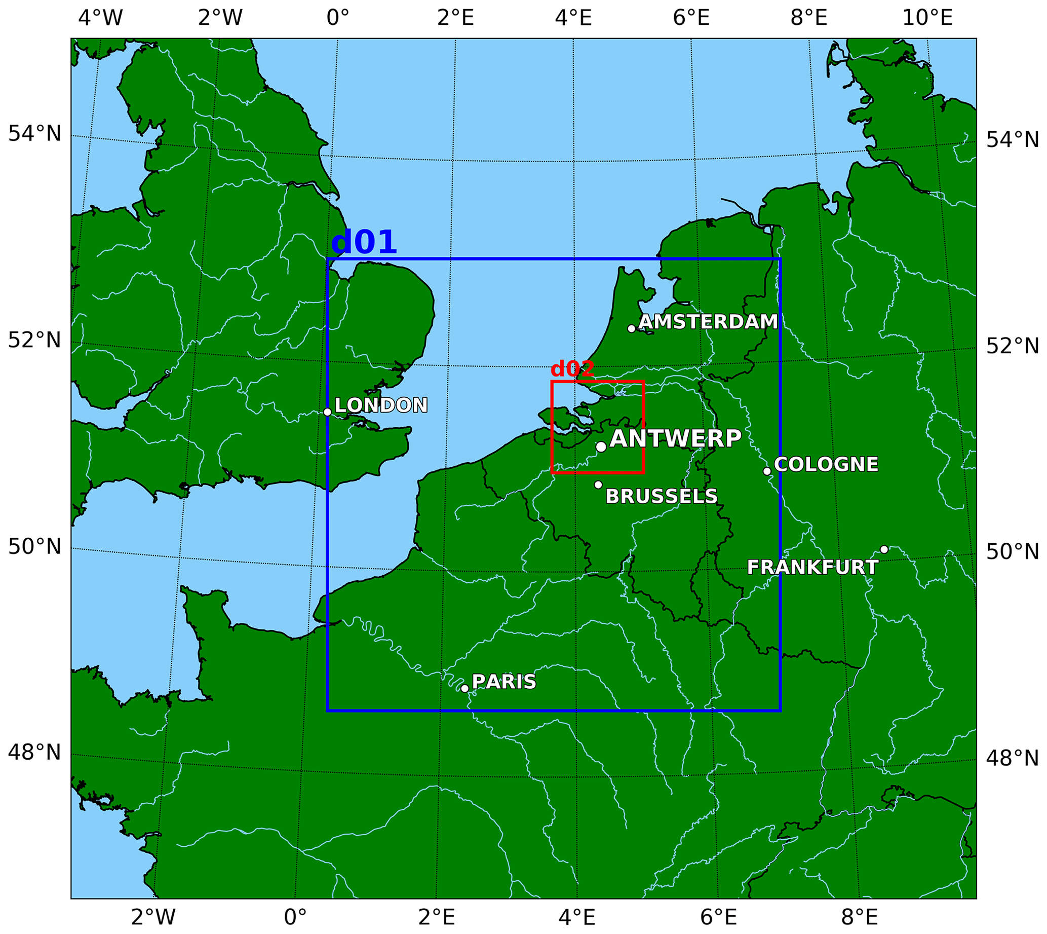
Figure 1 Map of western Europe, indicating the two model domains in blue (d01; 5 × 5 km² resolution) and red (d02; 1 × 1 km² resolution).

Longer (15 d) simulations were also conducted to evaluate the emissions and assess the longer-term model variability through comparisons with TROPOMI and surface concentration measurements. This simulation period extends from 15 June 2019 00:00 UT until 30 June 2019 00:00 UT. Each 15 d run was not set up to run continuously; instead, it consists of a series of partially overlapping runs of 2 d and 6 h. Each consecutive run reinitialized the meteorological initial conditions, while the chemical initial conditions were provided by the results of the previous run, except in the case of the initial run at the start of the simulation period.

2.1.2 Physical parameterizations

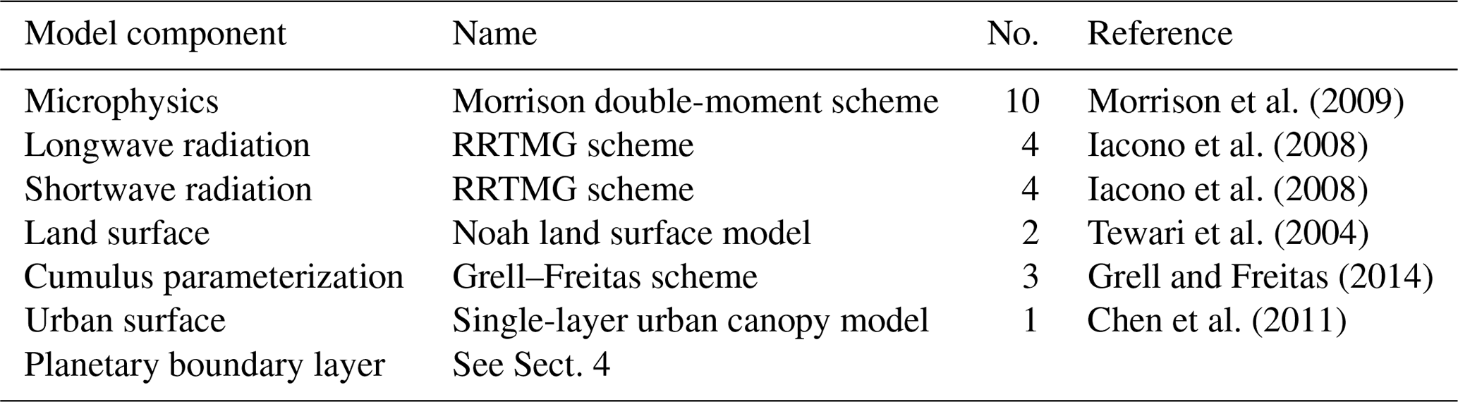
Many options are available in WRF for the parameterizations of physical processes. The basis for the choice of those parameterizations is borrowed from a previous high-resolution WRF-Chem study, conducted in Berlin in 2016 (Kuik et al., 2016), due to the similarity of the model setup and region of interest. The physical parameterization choices utilized in this study are listed in Table 1.

Table 1 List of WRF-Chem physical parameterizations adopted in this study. The number column refers to the parameterization choice as specified in the WRF-Chem model. Note: RRTMG is the Rapid Radiative Transfer Model for global climate models.

Due to the importance of planetary boundary layer (PBL) transport processes for the dispersion and vertical distribution of pollutants, the impact of the PBL parameterization on the model results was evaluated through further testing, as detailed in Sect. 4.

2.1.3 Chemical mechanism

The Carbon Bond Mechanism Z (CBM-Z; Zaveri and Peters, 1999) with the Kinetic PreProcessor (KPP) was chosen to simulate atmospheric gas-phase chemistry, and the Model for Simulating Aerosol Interactions and Chemistry (MOSAIC; Zaveri et al., 2008) is adopted for aerosols. The chemical reaction rates of the CBM-Z mechanism were updated in accordance with the latest recommendations of Jet Propulsion Laboratory (JPL) Publication 19-5 (Burkholder et al., 2020). VOC species mapping for the CBM-Z mechanism was done in conformity with previous studies (Chen et al., 2020).

2.1.4 Non-emission data

Static geographical data, such as land use category, vegetation and soil type, terrain height, etc., are downloaded from the WRF users' page (https://www2.mmm.ucar.edu/wrf/users/download/get_sources_wps_geog.html, last access: 9 January 2023) and are horizontally interpolated using the WRF Preprocessing System (WPS) onto the defined grid. The meteorological boundary and initial conditions for the model are obtained from the National Centers for Environmental Prediction (NCEP) Global Forecast System (GFS) analysis products (https://rda.ucar.edu/datasets/ds084.1/, last access: 9 January 2023). Those are provided as global GRIB2 files at 0.25^∘ × 0.25^∘ horizontal resolution and 6 h temporal resolution. Chemical boundary and initial conditions are mapped to the WRF grid using species concentrations from the Copernicus Atmosphere Monitoring Service (CAMS) global reanalysis (Inness et al., 2019a) for the species available (NO_x, CO, O₃, H₂O₂, HNO₃, C₂H₆, and peroxyacetyl nitrate, PAN), and the Community Atmosphere Model with Chemistry (CAM-chem) for the remainder (Lamarque et al., 2012; Emmons et al., 2020). CAMS and CAM-chem have 0.75^∘ × 0.75^∘ and 0.9^∘ × 1.25^∘ horizontal resolution, respectively. Both datasets were utilized using a 6 h temporal resolution.

2.2 Emissions

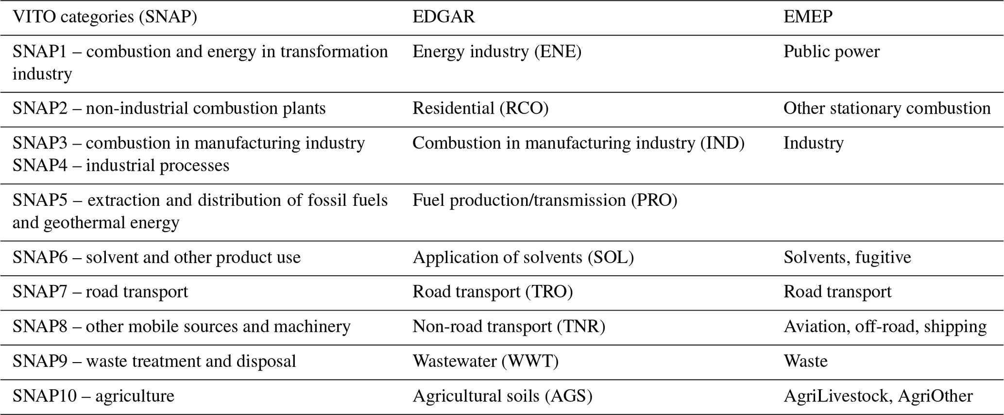
The emissions used in the model simulations originate from multiple datasets, both global and regional. High-resolution datasets (1 × 1 km²) are adopted for Flanders and the Netherlands, whereas comparatively coarser datasets (0.1^∘ × 0.1^∘) are used over the rest of the domain. Since each dataset has its own specific sector classification, homogenization of the sector types was done to allow for aggregation. The sector types (so-called Selected Nomenclature for Air Pollution, or SNAP, sectors) of the Flanders Environment Agency (VMM; Flanders Environmental Agency, 2017) dataset were adopted as the reference, and the sectors in the other inventories were mapped to the SNAP sectors, as illustrated in Table 2 for EDGAR (Emissions Database for Global Atmospheric Research) and EMEP (European Monitoring and Evaluation Programme). All emissions were processed for model input using the WRF-Chem preprocessing tool, anthro_emis, provided by the National Center for Atmospheric Research (NCAR). The monthly averaged distributions of NO_x, CO, non-methane volatile organic compounds (NMVOCs), and SO₂ anthropogenic emissions used in both domains of the model are illustrated in Fig. 2.

Figure 2 Emissions over the two model domains in their respective resolution (average for the period 15–30 June). The black square is the boundary of the inner domain (d02).

2.2.1 Flanders Emission Inventory (Flanders Environment Agency, VMM)

The Flemish Institute for Technological Research (VITO) processed emissions for CO, NH₃, total NMVOCs, NO_x (as NO₂), PM₁₀, and SO_x (as SO₂) over Flanders for 2017, split over 10 sectors, as originating from VMM. This inventory contains both gridded emissions over 1 × 1 km² and point source emissions corresponding to the industrial sector.

2.2.2 Dutch emissions inventory

High-resolution emissions over the Netherlands were obtained from the government of the Netherlands Pollutant Release and Transfer Register for all species in the VMM inventory (http://www.emissieregistratie.nl, last access: 9 January 2023). These are 1 × 1 km² resolution estimates representing the yearly total for 2017, split by sector and subsector. The species include NO₂, CO, NH₃, NMVOCs, PM₁₀, and SO₂. The data were regridded from their original projection into the VMM projection. The specifications of the VMM and Dutch emissions projections were obtained from their corresponding shapefiles in QGIS. The horizontal coordinates of the Dutch inventory cells were reprojected into the VMM grid using the Proj and pyproj.transform functions from the pyproj Python module (https://github.com/pyproj4/pyproj, last access: 9 January 2023).

2.2.3 EDGAR V4.3.2

The Emissions Database for Global Atmospheric Research (EDGAR) provides global sector-specific anthropogenic emissions on a 0.1^∘ × 0.1^∘ spatial grid. In this study, two different dataset versions have been used. From EDGAR v4.3.2 (Crippa et al., 2018; Huang et al., 2017), we use the annual disaggregated emissions of 25 NMVOC species and classes. The most recent year in this dataset is 2012, and this was used for the NMVOCs. Since only the total NMVOC emissions were available from the Flemish and Dutch inventories, the NMVOC speciation among different NMVOCs was obtained from EDGARv4.3.2 and combined with the high-resolution total NMVOC data over Flanders and the Netherlands.

2.2.4 EDGAR V5

Black carbon (BC) and organic carbon (OC) emissions were taken from EDGAR V5.0 2015 (Crippa et al., 2020), which are month specific. These emissions were utilized over both domains and regridded to the desired spatial resolution using the WRF-Chem preprocessor anthro_emis.

2.2.5 EMEP

Emissions from the European Monitoring and Evaluation Programme (EMEP, https://www.ceip.at/the-emep-grid/gridded-emissions, last access: 9 January 2023, European Monitoring and Evaluation Programme Centre on Emission Inventories and Projections, 2022) were used for NO_x, CO, PM_2.5, PM₁₀, and SO_x over Europe. These are yearly emissions gridded at 0.1^∘ × 0.1^∘ from 2012, provided as both a total emission and split by individual sector. Total NMVOC emissions are also available from EMEP but were not used as they are not speciated.

Table 2 Correspondence between the emission sectors of the SNAP, EDGAR, and EMEP inventories, as adopted in this work.

The total annual emissions in the model domain (d01) amount to 770 (NO), 1960 (CO), and 2170 Gg (NMVOC). Figure 3 shows the sector contributions for the total NO_x, CO, and NMVOC emissions over the entire model domain. The “other” category is a sum of the least contributing sectors (less than 1 % of the total emission). For NO_x, the dominant sectors are the SNAP sectors 7 (road transport) and 8 (mostly shipping), followed by the energy sector (SNAP1). For CO, industry (SNAP4) accounts for almost half of the total, while the transport (7+8) and residential (2) sectors account for most of the remainder. Contributions to NMVOC emissions come from all SNAP sectors, among which SNAP6 (solvents) is largely dominant, also from biogenic sources, more specifically in the form of biogenic isoprene that accounts for 23 % of the total NMVOC emissions.

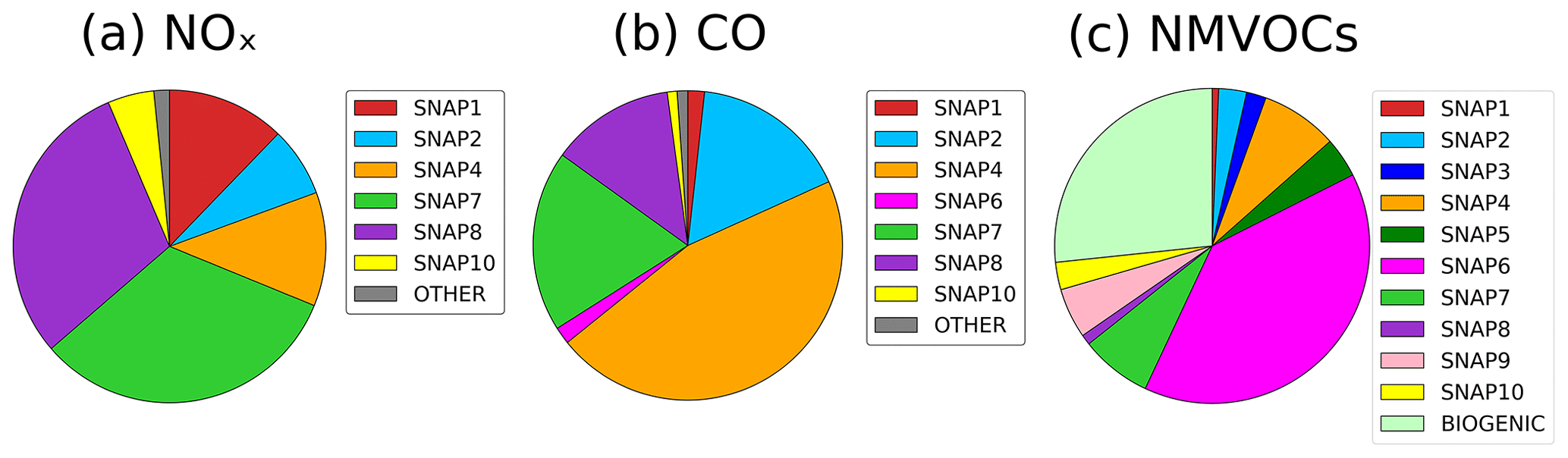
Figure 3 Sector contribution (%) to total emissions for NO_x (as NO), NMVOCs, and CO. Sectors with less than 1 % contribution are grouped into the “other” category, which differs between species.

2.2.6 Injection heights

Industrial emissions from the VMM inventory have vertical distribution information, namely the injection height, which ranges between 0 and 204 m. For other emission categories (except aircraft) and outside of Flanders, emissions are assumed to occur at surface level. The injection height information is used to populate the first three vertical levels of the emission input files (approximately 0–50, 50–110, 100–200 m a.g.l. – above ground level). Only 11 % of NO_x emissions from Flanders is injected above the first model layer (0–50 m; Sessions et al., 2011).

2.2.7 Aircraft and lightning

Global NO_x emissions from aircraft are provided from the CAMS-GLOB-AIR inventory (Granier et al., 2019), which is based on CEDS aircraft emission data (Hoesly et al., 2018). The data have a 0.5^∘ × 0.5^∘ horizontal resolution and monthly variation, with 25 vertical levels between the surface and 15 km altitude. The dataset used in this study is for the year 2019. To avoid double-counting, CAMS-GLOB-AIR emissions at the first level (closest to the surface) were omitted, since surface-level aircraft emissions are accounted for in the surface emission inventories.

Lightning-generated NO_x (LNOx) is computed within the WRF-Chem model through the additional physics parameterization for the lightning process, based on the PR92 scheme (Price and Rind, 1992). The amount of LNOx is determined from the lightning flash rate (parameterized based on the convective cloud-top height calculated by WRF), with different formulations for continental and marine thunderstorms.

2.2.8 Temporal variation in anthropogenic emissions

The surface emission inventories described in Sect. 2.2.1–2.2.5 generally ignore seasonal, weekly, and diurnal variations in anthropogenic emissions, which can, however, be significant. Diurnal, weekly, and seasonal cycles of emissions were included in the model based on the detailed sector-specific and country-specific temporal profiles of Crippa et al. (2020).

For each sector, the emission is modulated by a temporal factor, following Crippa et al. (2020), as described by Eq. (1). The temporal profiles pertain to the EDGAR sectors. The correspondence between the EDGAR and SNAP sector categories is displayed in Table 2.

$$\begin{array}{}\text{(1)}& \mathrm{TF}={\mathit{\alpha }}_{\mathrm{s},\mathrm{d},\mathrm{h}}\times {\mathit{\beta }}_{\mathrm{s},\mathrm{w}}\times {\mathit{\gamma }}_{\mathrm{s}},\end{array}$$

where TF represents the temporal factor made up of its three components, i.e., a diurnal factor, α, dependent on sector, day type (weekday, Saturday, or Sunday), and hour, represented by subscripts s, d, and h, respectively. β stands for the daily factor, dependent on the sector (s) and day of the week (w). The final component is the monthly factor γ. Each component is country dependent. We adopted the temporal profiles provided for Belgium, which are very similar to those for the neighboring countries. Each of the temporal variations is also month dependent. Simulations were conducted in the month of June. Temporal variation was not applied to the aircraft emissions, as these do not correspond to an EDGAR category.

Figure 4 shows the temporal features of different sectors over the last 2 d of the 3 d runs, namely 28 and 29 June 2019, corresponding to a Friday and a Saturday. The time series shows a distinct diurnal cycle for each of the categories and distinctly lower emissions on 29 June due to the weekend effect. SNAP9 is not shown in this figure, as it has no temporal variation.

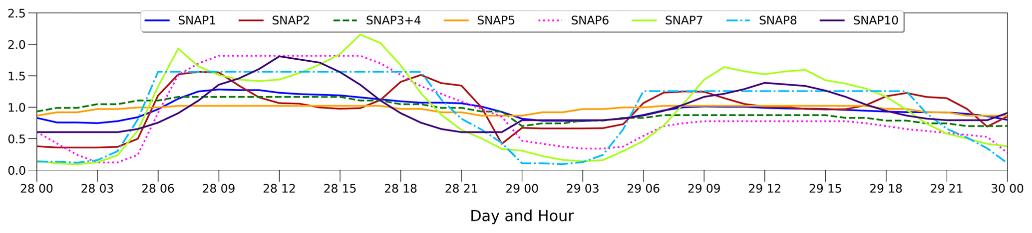
Figure 4 Temporal profile of SNAP categories over Friday (28 June) and Saturday (29 June), showing a variation in diurnal shape for the different sectors and over the 2 d. The time is indicated as local time or UTC+2.

The temporal profile of road transport (SNAP7) shows a minimum at the early hours of the day on both Friday and Saturday and two distinct peaks on Friday corresponding to the rush hours. Non-road transport (SNAP8) shows a constant value during the daytime for both Friday and Saturday. The shape for the non-industrial combustion sector (SNAP2) shows two broad peaks between 6:00 and 11:00 LT (local time) and 17:00 and 23:00 LT, corresponding to the hours before and after work, when there is more activity within the home. The industrial sectors (SNAP1, SNAP3+4, SNAP5, and SNAP6) generally have flatter curves, indicating a more constant release of emissions throughout the day.

All subsequent simulation results have incorporated the temporal profiles in the emission input.

2.2.9 Biogenic emissions

Biogenic emissions of VOCs and NO_x are calculated online in WRF-Chem using the algorithms of the Model of Emissions of Gases and Aerosols from Nature (MEGAN; Guenther et al., 2012). The emissions depend on meteorology (as calculated by WRF) and on emission factors and land use/land cover parameters provided as input at approximately 1 km resolution. Biogenic isoprene emissions total 676.5 Gg yr⁻¹ over the large domain.

3 Methodology

3.1 Meteorological data

3.1.1 Ground based

The Royal Meteorological Institute of Belgium (RMI) operates a network of automatic weather stations over the Belgian territory, recording near-surface meteorological observations, specifically temperature, relative humidity, air pressure, precipitation, global solar irradiance, wind speed, and wind direction. The measurements are obtained automatically every hour. Data were acquired for the month of June 2019 for two stations in the Antwerp area, namely Stabroek (51.3493^∘ N, 4.3789^∘ E) and Sint-Katelijne-Waver (51.0696^∘ N, 4.5346^∘ E). The location of the stations is indicated in Fig. 5. Both stations are within the inner domain within the Antwerp area (https://www.meteo.be/en/about-rmi/observation-network/automatische-weerstations, last access: 9 January 2023).

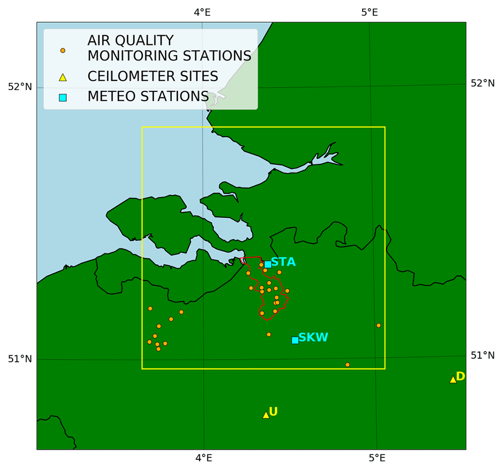
Figure 5 Map showing the geographical location of different in situ data measuring sites. The meteorological (blue square) and air quality (orange circle) sites are in the innermost domain, indicated by the yellow square, while the ceilometer stations (yellow triangle) are in the surrounding area. The red outline represents the Antwerp municipality.

3.1.2 Radio- and ozonesonde

Ozonesondes are balloon-borne instruments measuring ozone concentration as they travel from the surface to altitudes of around 30 km in the mid-stratosphere. The type of ozonesonde currently used by the RMI at the Uccle station (50^∘48^′ N, 4^∘21^′ E, 100 m above sea level (a.s.l.), indicated by “U” in Fig. 5) is an electrochemical concentration cell (ECC) sonde which measures ozone concentration through a reaction with ambient air in an electrochemical cell that generates an electric current proportional to the amount of ozone in the air (Van Malderen et al., 2021; Deshler et al., 2017). These are systematic measurements conducted roughly every 3 d. We compared the model with sonde data for the 28 June. Alongside ozone, air temperature, relative humidity, wind direction, and wind speed information are measured with the radiosonde that the ozonesonde is coupled with. Those airborne instruments take measurements during its ascent to and descent from the maximum altitude, and the horizontal coordinate path of the balloon can be reconstructed using the measured wind speed, wind direction, and time passed from the start of measurements.

3.1.3 Ceilometer

There are four automatic lidar (light detection and ranging) ceilometer (ALC) monitoring stations in Belgium that have been set up by the RMI to measure the cloud base height and mixing layer height (https://ozone.meteo.be/instruments-and-observation-techniques/lidar-ceilometer, last access: 9 January 2023). The Vaisala CL51 instrument emits a single-wavelength pulse vertically into the atmosphere and measures the time taken for a backscattered signal to return, proportional to the size and scattering cross section of molecules and particles (Haeffelin et al., 2016). The planetary boundary layer height (PBLH) is retrieved from ceilometer measurements by applying a similar approach to that used in Pal et al. (2013). The retrieval algorithm is based on the 2D gradients method (Haeffelin et al., 2012) in combination with the variance method (Menut et al., 1999). The retrieved PBLHs are available for the month of June 2019 at 10 min intervals and are checked for quality following the methodology used in De Haij et al. (2007). In case of rain/fog, the retrieved PBLH is not used. For all other sky conditions, a quality criteria equal to 0.85 was used, and a value higher than 0.85 is an indication of an incorrect retrieved PBLH. We use measurements obtained at the stations of Uccle (50.7975^∘ N, 4.3594^∘ E) and Diepenbeek (50.9155^∘ N, 5.4503^∘ E). These stations are indicated in Fig. 5, where each station is labeled by its initial.

3.2 In situ surface chemical observations

The Belgian Interregional Environmental Agency (IRCEL-CELINE) hosts air quality measurement stations, providing time series of hourly measurements of common pollutant concentrations (NO₂, NO, CO, and O₃). The 27 stations used for the evaluation of the model are those located within the inner model domain (Fig. 5) listed in Table S1 in the Supplement. When comparing the modeled NO₂ concentration with station data, a correction factor (F_int) is applied (either to the observations or to the model results) to correct for the known existence of interferences in the chemiluminescence NO₂ measurement due to NO_y reservoir compounds including HNO₃ and PAN (Lamsal et al., 2008). More precisely, in most instances, the modeled NO₂ concentrations are multiplied by the correction factor (F_int) given by the following:

$$\begin{array}{}\text{(2)}& F_{\mathrm{int}}=\mathrm{1}+{\displaystyle \frac{\mathrm{0.95}\times \left[\mathrm{PAN}\right]+\mathrm{0.35}\times \left[{\mathrm{HNO}}_{\mathrm{3}}\right]}{\left[{\mathrm{NO}}_{\mathrm{2}}\right]}},\end{array}$$

where [NO₂], [PAN], and [HNO₃] are the modeled mixing ratios of NO₂, PAN, and HNO₃. In other words, the measurements are being compared to interference-corrected NO₂ concentrations, hereafter denoted as NO${}_{\mathrm{2}}^{*}$. Alternatively, the modeled NO₂ could be compared to the measured concentrations divided by F_int in order to remove the estimated interference contribution from the measurements. Because the correction F_int involves model-calculated concentrations, however, this procedure is inappropriate when evaluating multiple model runs against NO₂ data.

3.3 APEX

NO₂ tropospheric vertical column densities (VCDs) were retrieved over Antwerp during two flights utilizing hyperspectral Airborne Prism EXperiment (APEX) observations, as part of the S5P validation campaign over Belgium (S5PVAL-BE). The APEX instrument is a pushbroom hyperspectral imager that integrates spectroscopy and 2-D spatial mapping in high resolution (∼ 75 m × 120 m). APEX utilizes backscattered solar radiation over a wavelength range of 370 to 2540 nm. The flights over Antwerp took place on 27 and 29 June 2019, using the APEX instrument aboard a Cessna 208B Grand Caravan EX at an altitude of 6.5 km a.g.l. The days on which the flights took place were chosen for their good visibility due to cloud-free conditions. The flight times were chosen to coincide within 1 h of the times of the S5P overpasses on the corresponding days. Each APEX NO₂ column is provided with vertically resolved box air mass factors (AMFs) estimated from radiative transfer calculations. The total AMF, equal to the ratio of the slant column to the vertical column, is computed by vertically integrating the box AMFs along the a priori NO₂ profile. This profile is taken to be a constant mixing ratio in the PBL and zero in the free troposphere, with the PBL height being obtained from ceilometer data in Uccle, near Brussels (Tack et al., 2017, 2021). The averaging kernels (A_l, with l as the vertical level) required for comparison of model data with APEX columns are calculated as the ratio of the box AMFs to the total AMF (Eskes and Boersma, 2003). APEX columns and averaging kernels are regridded at the 1 km² WRF resolution. The model NO₂ columns are computed by vertically integrating the model partial columns (below the tropopause and mapped onto the APEX vertical grid) multiplied by the averaging kernels.

3.4 TROPOMI

The TROPOspheric Monitoring Instrument (TROPOMI) was launched aboard the European Space Agency (ESA) S5P satellite in 2017 to monitor and quantify air quality across the globe (Veefkind et al., 2012). S5P is a near-polar, sun-synchronous satellite, with a local overpass time at 13:30. TROPOMI is a nadir-viewing pushbroom imaging spectrometer with ultraviolet (UV), visible (VIS), near-infrared (NIR), and shortwave infrared (SWIR) spectral bands, which allow for measuring atmospheric constituents such as nitrogen dioxide (NO₂), ozone (O₃), carbon monoxide (CO), and other compounds at the high spatial resolution of 7 km × 3.5 km (5.5 km × 3.5 km since August 2019). The retrieval of tropospheric NO₂ is a three-step process. First, a differential optical absorption spectroscopy (DOAS) method is used to obtain the total slant column density of NO₂ from the Level-1b radiance and irradiance spectra measured by TROPOMI. This method utilizes a spectral range of 405–465 nm and is based on the nonlinear fitting approach for OMI (van Geffen et al., 2020). The second step requires a separation of tropospheric and stratospheric NO₂, which is realized using the data assimilation of slant columns with the TM5-MP chemistry transport model (Williams et al., 2017). Finally, the tropospheric slant column density, derived in the previous step, is converted to a tropospheric vertical column density using precalculated air mass factors (AMFs). AMFs are obtained from radiative transfer calculations using NO₂ vertical profiles from the TM5-MP chemistry transport model. The NO₂ retrieval and the individual steps are described in further detail in the TROPOMI ATBD (Algorithm Theoretical Basis Document) of the total and tropospheric NO₂ data products (van Geffen et al., 2018). To enable the comparison between TROPOMI and WRF-Chem, the model NO₂ columns are computed at the WRF-Chem resolution by the convolution of the modeled tropospheric partial columns with the TROPOMI averaging kernels. The resulting columns are then regridded onto the TROPOMI resolution, using the latitude and longitude coordinates of the four corners of each TROPOMI cell. The quality filter (QF) recommended by the TROPOMI ATBD is applied to both model and measurements, i.e., only pixels with QF >0.75 are kept for further analysis.

We present model evaluations against the standard L2 tropospheric NO₂ product (OFFL v1.3.1) and against the newly released PAL reprocessing based on version 2.3.1 of the operational processor (https://data-portal.s5p-pal.com/product-docs/no2/PAL_reprocessing_NO2_v02.03.01_20211215.pdf, last access: 9 January 2023; van Geffen et al., 2022) available for download from the S5P-PAL data portal (https://data-portal.s5p-pal.com/products/no2.html, last access: 9 January 2023). Hereafter, those products will be noted TROPOMI_v1.3 and TROPOMI_PAL, respectively.

4 Results

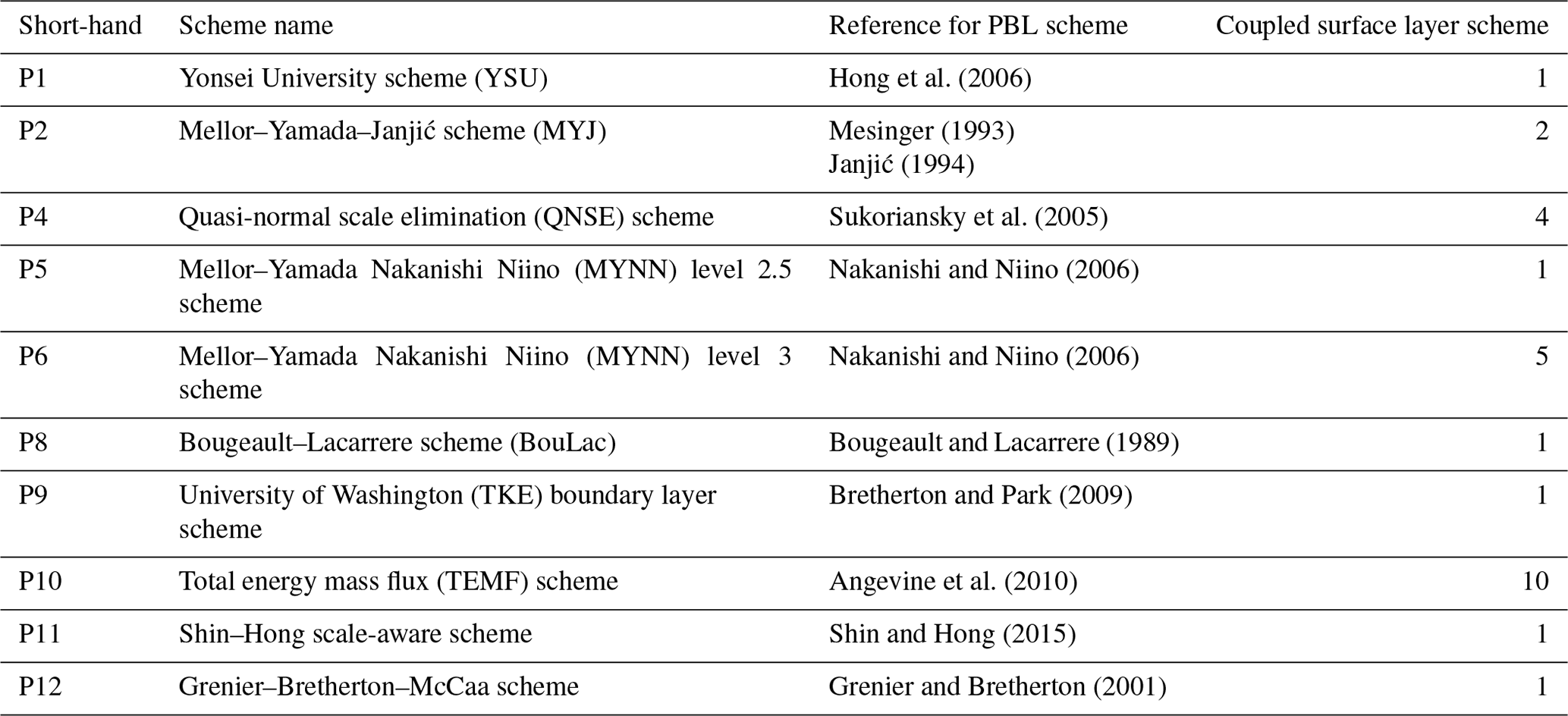
Given the important role of the PBL parameterization in the simulation of atmospheric composition, the PBL scheme was varied in the evaluation of WRF-Chem performance against measurements. A total of 10 PBL schemes were tested, and these are listed in Table 3. The shorthand notation refers to the model simulation utilizing the corresponding PBL scheme. The P4 run crashed before completion for unknown reasons (it stopped around 04:30 LT on 29 June), which is why the data series is incomplete for multiple plots. The choices of the PBL scheme and surface layer parameterization are coupled, and the suitable pairs are suggested in the WRF User's Guide V4 (https://www2.mmm.ucar.edu/wrf/users/docs/user_guide_v4/contents.html, last access: 9 January 2023). When several choices are possible for a given PBL scheme, the effect of the choice of surface layer scheme was tested through comparison with meteorological data. The results indicate very little sensitivity to the choice of surface layer scheme. Surface layer option 1 (revised MM5 Monin–Obukhov scheme; Jiménez et al., 2012) was selected in cases where multiple choices were proposed in order to ensure the best consistency amongst the different runs. The surface layer scheme options chosen for each simulation are listed in Table 3.

In all comparisons shown in this section, the time refers to local time, i.e., UTC+2.

Table 3 List of WRF-Chem planetary boundary layer parameterizations and their coupled surface layer scheme tested in this study. The number in the last column identifies the surface layer scheme, as defined in the WRF documentation (Skamarock et al., 2019). Note that schemes 7 and 99 were not tested, as scheme 7 appears incompatible with the other physical parameterizations used, and scheme 99 will be removed in future versions of the model.

4.1 Comparisons with meteorological observations

4.1.1 Ceilometer

The PBL height (PBLH) from WRF-Chem was compared with ceilometer measurements from Uccle and Diepenbeek (labeled “U” and “D” in Fig. 5) over the 3 d simulation period. The retrieved PBLH are split into two categories based on the quality criteria. They are shown in Fig. 6 as green dots (good-quality data; QF <0.85) and brown dots (low quality). The measured data and corresponding model output were averaged over the two locations.

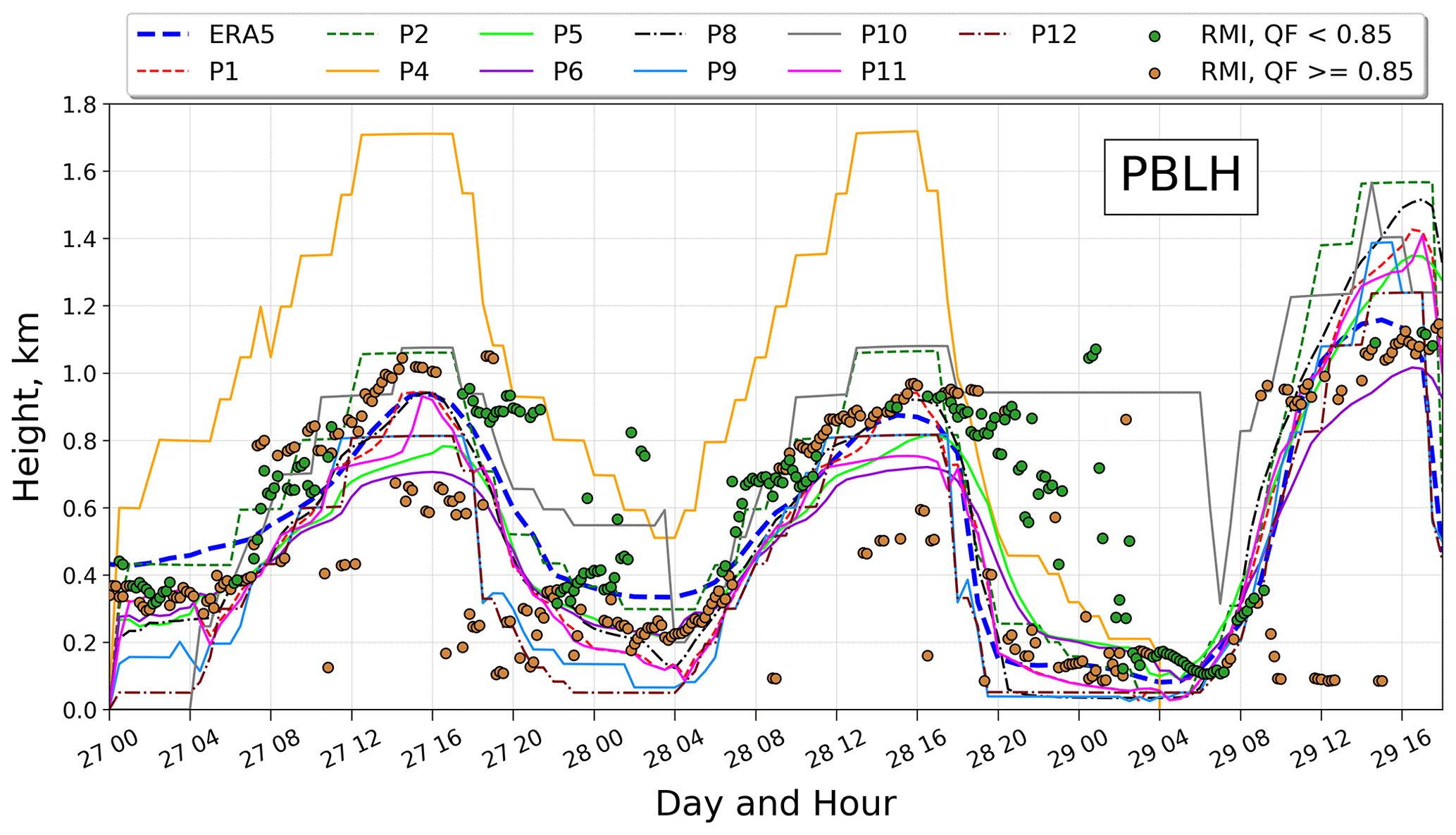
Figure 6 Time series of measured and modeled PBL height between 27 and 29 June 2019 (average of two sites). Good-quality measurements (QF <0.85) are shown as green dots and low-quality data (QF >0.85) as brown dots. The dark blue dashed line is the PBL height from the ERA5 reanalysis (Hersbach et al., 2020). The other curves represent the WRF model output for each of the boundary layer schemes listed in Table 3.

Generally, the different PBL parameterization runs are able to reproduce the observed temporal shape of PBLH, especially during the daytime hours (8:00–18:00 LT). All schemes perform well regarding the time (∼ 16:00 LT) and approximate magnitude (1 km) of the maximum PBLH. However, most schemes underestimate the PBL height during the nighttime (20:00–4:00 LT), especially when compared with the good quality ceilometer data. The extent of the underestimation varies between the different PBL schemes. P10 is a noticeable exception, as it consistently overestimates the observations during the night. Both P9 and P12 predict a sharp drop in PBLH around 18:00 LT (not seen in the observations) and exhibit the lowest PBL height for both nights. However, the relatively high observed PBLH in the late afternoon might be an artifact due to the persistence of a residual aerosol layer which does not subside rapidly despite the weakening of turbulence at that time (Haeffelin et al., 2012). There are clear outliers among the different schemes – P4 performs the worst as its PBLH far exceeds the height of the measurements. Besides P9 and P12 (of which poor performance might partly be due to the limited reliability of ceilometer data in the late afternoon), P4 and P10 exhibit the poorest statistics (correlation, root mean square error, RMSE, and mean bias, MB) among the different schemes (see Table S2 in the Supplement).

4.1.2 Surface meteorology

Figure 7 presents the time series of meteorological parameters observed and simulated by the model in the region of Antwerp (average of two stations, namely Stabroek and Sint-Katelijne-Waver). The model follows the observed diurnal shape of surface temperature very well, with Pearson's R² values above 0.98 for every simulation except P6 (too cold in the afternoon and night) and P10 (too warm in the morning). The nighttime temperature from WRF-Chem is slightly but consistently underestimated by all schemes, whereas the agreement between the modeled and observed temperature is generally excellent during the daytime. P6 and P10 are among the worst-performing PBL schemes for correlation, RMSE and mean bias (Table S2). P4 also displays a large negative bias.

Similar to temperature, the measured relative humidity exhibits a diurnal shape that WRF-Chem is able to simulate, with a maximum during the nighttime and lower values during the day. As for temperature, P4, P6, and P10 are the worst-performing runs. Those three schemes overestimate the relative humidity, especially P6 during the day (by more than 10 %) and P10 during the night. P9 is consistently too dry.

The observed solar irradiance reveals essentially clear-sky conditions during the 3 d. This is well reproduced by most PBL runs, except P6, which underestimates the solar irradiance between 21:00 and 0:00 LT on the first 2 d, likely due to cloudiness, and is in line with the overly moist conditions calculated by this scheme. To a lesser extent, P5 also slightly underestimates the solar irradiance on 28 June between 18:00 and 0:00 LT.

Among the meteorological variables, wind speed displays the most variability between the different PBL runs and the highest discrepancy with the measurements. Wind speed is overestimated by all schemes. The overestimation is highest for P2 and P4, while P10 also performs poorly for both wind speed and wind direction. The other schemes perform similarly, with a moderate wind speed bias of ∼ 1.1 m s⁻¹ and a correlation of ∼ 0.85 for wind direction. Similar wind speed overestimations have been noted in previous WRF-Chem evaluation studies over urban areas (e.g., Feng et al., 2016; Kim et al., 2013). Note that the single-layer urban canopy model (UCM) used in our study as an urban surface model (Table 1) has been found by those studies to provide the best results, based on comparisons with ceilometer and wind measurements over cities. Overall, those comparisons for the surface meteorological variables indicate a good model performance, except for the few outliers that consistently perform poorly, which are mainly P4, P6, and P10.

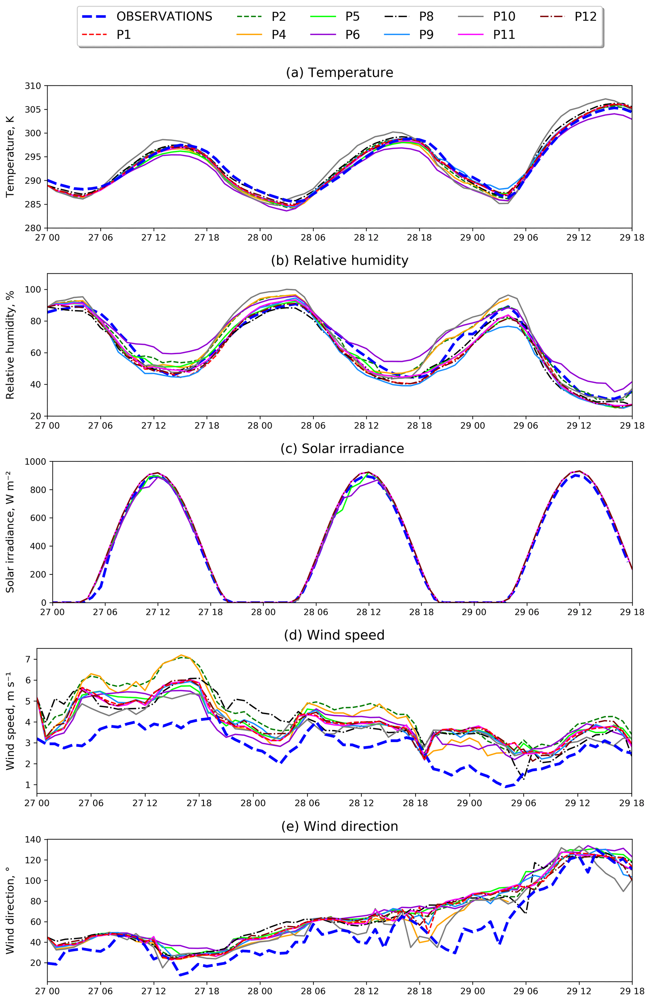
Figure 7 Observed and modeled evolution of surface meteorological parameters on 27–29 June 2019. (a) Temperature, (b) relative humidity, (c) solar irradiance, (d) wind speed, and (e) wind direction. The dark blue dashed line represents the observations, averaged over the two measuring sites, while the other lines represent the output from the model sensitivity runs, labeled in the legend (see Table 3).

4.1.3 Sonde

Variation in the output of the PBL runs occurs only in the lowest part of the troposphere (<1200 m). The meteorological output of the different schemes is very similar at higher altitudes. The model succeeds very well in reproducing the vertical profile of meteorological parameters in the free troposphere (Fig. 8), especially temperature and wind. The model underestimates ozone between 3 and 10 km altitude but agrees very well with the sonde in the lowest layers. To a large extent, the discrepancy in the upper troposphere is due to underestimated ozone mixing ratios by the CAMS analysis for this date (also shown in Fig. 8e). CAMS ozone is used to specify the initial and lateral boundary conditions in the model.

The impact of the PBL option on the comparisons between the simulated and measured data is examined below approximately 1200 m altitude. Both sonde ascent and descent are considered; the average of the two is plotted in Fig. 9, and the combined data are used to calculate the statistics in Table S2. Most of the runs slightly overestimate the temperature in the lowermost 600 m. As with the surface data, P6 is an outlier in that it displays the highest, negative mean bias. P8 and P10 have the highest positive biases. These findings are consistent with the surface temperature comparison.

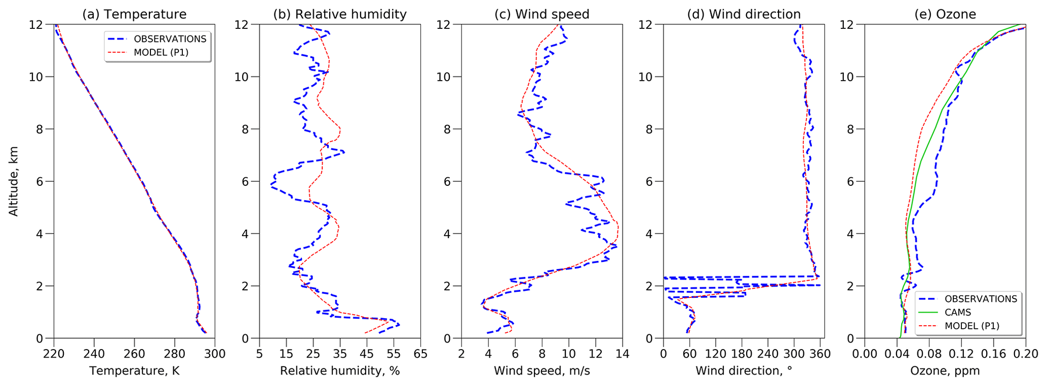
Figure 8 Vertical profile of meteorological parameters and ozone mixing ratio measured by ozonesonde on 28 June 2019 (dashed blue line) and calculated by WRF-Chem (red dotted line), shown between 0 and 12 km (approximate tropopause height) for one PBL scheme (P1). The ozone profile from the CAMS analysis (green) is also shown in panel (e).

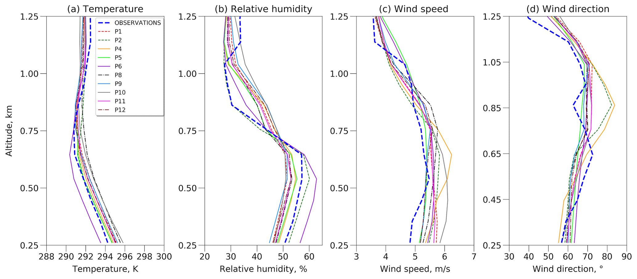
Figure 9 Vertical profile of meteorological parameters (thick blue line) observed by a radiosonde on 28 June 2019 below 1.25 km altitude and WRF-Chem results for different boundary layer parameterizations (see Table 3).

Although all runs follow the general shape of the relative-humidity-measured profile, the vertical gradient between 700 and 1000 m is generally underestimated by the model. P2 is the exception, which provides the best overall agreement with the measurements (Table S2). The largest biases are found for P6 (too moist in the lowest layers) and for P10 (highest overestimation above 800 m).

All PBL schemes overestimate the wind speed at near-surface altitudes, which is consistent with the surface data. P2 and P4 show a large positive bias in wind direction (ca. +20^∘) around 900 m altitude and are generally the worst-performing schemes for both wind speed and wind direction, with the lowest correlations and highest RMSE values. P8 shows the best performance statistically, despite being amongst the worst-performing options for the surface wind speed. Besides P2 and P4, most of the schemes display similar statistics (Table S2).

4.2 Comparisons with surface chemical observations

4.2.1 Role of PBL scheme in model comparison with surface NO₂ data

The output of the test runs was further compared against measured surface NO₂ at the IRCEL-CELINE stations located in the inner domain. The modeled values shown in Fig. 10 have been corrected to account for the interference of other NO_y species in the measurements, as described in Sect. 3.2. To help with interpreting these comparisons, Fig. 11 displays the vertical profiles of modeled NO₂ mixing ratios in the early afternoon (13:30 LT on 27 June) and during the night (01:30 LT on 28 June) below 1.4 km altitude. Note that the choice of PBL scheme has essentially no impact above that altitude.

Figure 10 Evaluation of modeled NO${}_{\mathrm{2}}^{*}$ concentrations (corrected to account for interference of other NO_y species; see the text) using station data over the 3 d simulation period. Both the model data and observations are averages over 24 stations within the inner domain. The thick dashed line represents the measurements, while the other curves represent the different PBL runs. The vertical dashed lines separate night- and daytime, shaded in blue and orange, respectively.

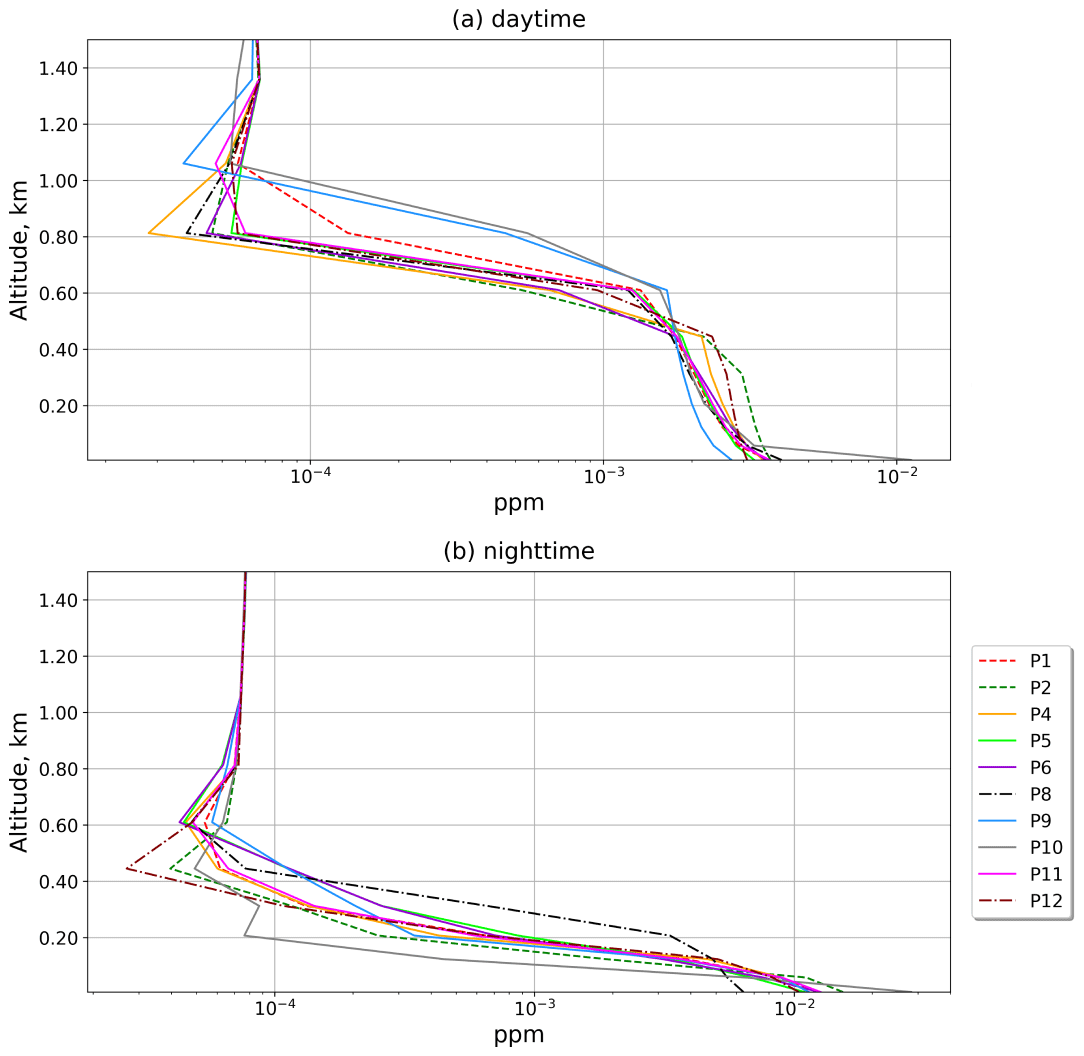
Figure 11 Average NO₂ vertical profile over the APEX region, shown for all sensitivity simulations below 1.4 km altitude (a) at 13:30 UT on 27 June and (b) at 01:30 UT on 28 June. Above 1.4 km, the differences between model sensitivity runs are negligible.

Similar to the comparison with meteorological parameters, most of the PBL options are cohesive in their performance against observations, except for four outliers. P10 consistently overestimates NO₂ over the 3 d period by a factor of ∼ 2. This overestimation is associated with a very steep vertical gradient of NO₂ concentration within the PBL (see Fig. 11) which suggests insufficient boundary layer turbulent mixing. The schemes P2 and especially P4 lead to high RMSE and MB values (Table S3), consistent with their relatively lower performance at simulating meteorology, particularly the wind. P8 exhibits the least-pronounced diurnal cycle of NO₂ concentration, which is in better agreement with the observations than the other simulations. Excluding P4 and P10, surface NO₂ exhibits an average bias between −4.3 % and −25 % during daytime (6:00–20:00 LT) and overestimations of 8.2 %–77 % for nighttime concentrations. On 27 and 28 June, all remaining schemes generally underestimate the NO₂ concentrations during daytime hours and overestimate NO₂ at night, highlighting a potential issue with the diurnal profile of NO₂ in the model. Possible causes for this pattern, including issues with PBL vertical transport and with the chemical sinks of NO₂, will be discussed in the next subsections. On 29 June, however, most schemes perform very well. The larger daytime biases on weekdays (27–28 June) compared to Saturday (29 June) for all runs (except P10) suggest an issue with the weekly cycle of emissions, which is further explored in Sect. 4.2.5. Based on these results and on the comparisons with meteorological measurements, the PBL options P2 (MYJ), P4 (QNSE), P6 (MYNN Level 3) and P10 (TEMF) are considered less reliable for simulating air composition over Antwerp and the surrounding areas and are therefore not recommended.

Due to computational resource limitations, we adopt only one PBL option (P1, the YSU scheme) for the 15 d simulations. The choice is justified by the good performance of the P1 simulation across all meteorological comparisons. In addition, it compares similarly to most other schemes against surface NO₂ data, when excluding the few outliers noted above. The P8 scheme (BouLac) could have been a meaningful alternative choice given its better agreement against surface NO₂ data. Note, however, that the lower amplitude of the diurnal cycle of surface NO₂ simulated with P8 might be partly due to the near-absence of the diurnal cycle in the wind speed obtained with that scheme (Fig. 7), whereas the observations and most other model simulations indicate higher wind speeds during the day than during the night. Since high wind speeds cause faster export and dilution of pollution plumes, and since the IRCEL-CELINE stations are mostly located within source regions, the better correlation of P8 with NO₂ data might be partly fortuitous. Furthermore, as shown in Fig. 11, the NO₂ daytime vertical profiles calculated with P1 and P8 are very close, implying very similar NO₂ column amounts. The choice of P1 or P8 as a PBL option should therefore not have a large impact on WRF-Chem comparisons with APEX or TROPOMI data.

4.2.2 Evaluation of the 15 d model simulation against NO_x, CO, and O₃ station data

A comparison of the 15 d model simulation with measured surface NO${}_{\mathrm{2}}^{*}$, NO, CO, and O₃ data is shown in Fig. 12. The concentrations were averaged over all stations within the inner domain for which measurements are available for the corresponding species. The spatial distribution of the NO₂-measuring stations is shown in Fig. 13. Both interference-corrected (NO${}_{\mathrm{2}}^{*}$) and uncorrected NO₂ concentrations are shown in Fig. 12. Simulated NO${}_{\mathrm{2}}^{*}$ generally follows the diurnal trends seen in the IRCEL-CELINE data, with peaks generally found during the nighttime hours and lower values occurring during the daytime. There is a consistent model underestimation of daytime NO₂, although the Lamsal et al. (2008) correction intended to account for interferences in NO₂ measurements improves the agreement between simulated and observed daytime concentrations. The average model bias for daytime hours (9:00–17:00 LT) is −28 % and −40 % with and without this correction, respectively. Figure 13 illustrates the spatial distribution of the median (modeled/observed) concentrations among the individual stations. The highest underestimation is found at urban stations, e.g., Borgerhout within the city of Antwerp (time series shown in Fig. S1 in the Supplement), where an underestimation of −75 % is seen during daytime hours. A large negative bias (−60 %) is also found in the Ghent city center. This might indicate an underestimation of traffic emissions under urban driving conditions or a misrepresentation of transport/mixing in large cities, such as street canyon effects (Scaperdas and Covile, 1999). The model underestimation is very low at stations further away from emission sources, as is the case with the Schoten (“S” in Fig. 13) background station (median ratio = 0.97; see also Fig. S1). Besides the urban stations, the median ratio ranges between 0.6 and 1.1 during the daytime.

Nighttime surface NO${}_{\mathrm{2}}^{*}$ is overestimated at all stations except Borgerhout, with the median ratios ranging between ∼ 1.2 and 1.8. This overestimation indicates insufficient loss due to vertical mixing and/or chemical sink during the night. For example, the heterogeneous conversion of NO₂ to HONO and HNO₃ on surfaces at the ground or on aerosols (Kleffmann et al., 2003) is not represented in the model. However, this sink should not strongly impact the nighttime NO₂ levels, since the reported conversion rates based on in situ measurements do not exceed ∼ 2 % h⁻¹ and generally fall below 1 % h⁻¹ (Kleffmann et al., 2003; Hu et al., 2022). Flaws in the parameterization of vertical transport are suggested by the model underestimation of PBL height during nighttime (Sect. 4.1.1), in particular for the P1 parameterization. Insufficient vertical mixing at night is also suggested by comparison of the observed and measured diurnal cycle of CO concentration, which is presented in the next subsection.

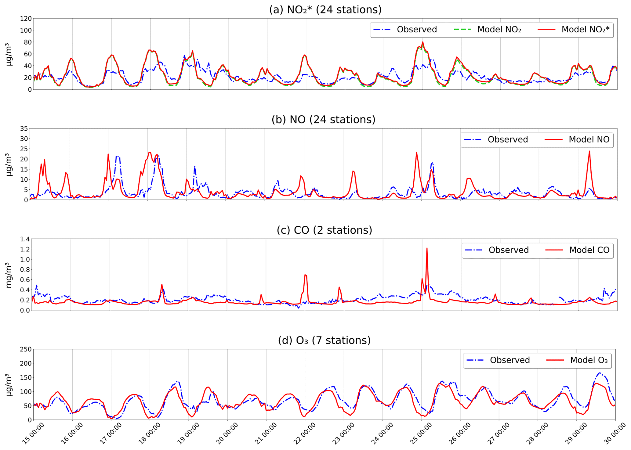
Figure 12 Time series of observed and modeled concentrations of (a) NO${}_{\mathrm{2}}^{*}$, (b) NO, (c) CO, and (d) O₃ at IRCEL-CELINE network stations for the 15 d duration of the reference simulation. Each time series is an average of measurements at the available stations for the corresponding species. Interference-corrected model NO₂ (NO${}_{\mathrm{2}}^{*}$) is shown in red and uncorrected NO₂ in green.

Figure 13 Median (a) daytime and (b) nighttime ratio (model/observation) of NO${}_{\mathrm{2}}^{*}$ concentrations at IRCEL-CELINE stations in the inner domain. Points “A”, “B”, and “S” denote the stations Antwerpen, Borgerhout, and Schoten.

The $\mathrm{NO}/{\mathrm{NO}}_{\mathrm{2}}$ ratio (RNOx) from both the model and observations are compared in Fig. 14. In this instance, the modeled NO₂ concentrations are uncorrected, and the measurements are corrected for interferences, as described in Sect. 3.2. The modeled ratios match the observations very well, except for a substantial overestimation (factor of 2) on 29 June. The modeled RNOx closely follows the photochemical steady state (PSS) defined by assuming equilibrium between the NO_x interconversion reactions, as follows:

$$\begin{array}{}\text{(R1)}& {\displaystyle }\mathrm{NO}+{\mathrm{O}}_{\mathrm{3}}\to {\mathrm{NO}}_{\mathrm{2}}+{\mathrm{O}}_{\mathrm{2}}{k}_{\mathrm{1}}\text{(R2)}& {\displaystyle }\mathrm{NO}+{\mathrm{HO}}_{\mathrm{2}}\to {\mathrm{NO}}_{\mathrm{2}}+\mathrm{OH}{k}_{\mathrm{2}}\text{(R3)}& {\displaystyle }\mathrm{NO}+{\mathrm{RO}}_{\mathrm{2}}\to {\mathrm{NO}}_{\mathrm{2}}+\text{products}{k}_{\mathrm{3}}\text{(R4)}& {\displaystyle }{\mathrm{NO}}_{\mathrm{2}}+hv\to \mathrm{NO}+\mathrm{O}{J}_{{\mathrm{NO}}_{\mathrm{2}}}.\end{array}$$

NO is chemically converted into NO₂, mainly through reactions with O₃, HO₂, and organic peroxy radicals (RO₂), while NO₂ undergoes photolysis to produce NO and (upon reaction of atomic oxygen with O₂) O₃. The rates are obtained from the chemical mechanism in the model. RNOx at PSS is calculated using the following:

$$\begin{array}{}\text{(3)}& {\left({\displaystyle \frac{\left[\mathrm{NO}\right]}{\left[{\mathrm{NO}}_{\mathrm{2}}\right]}}\right)}_{\mathrm{PSS}}={\displaystyle \frac{J_{{\mathrm{NO}}_{\mathrm{2}}}}{k_{\mathrm{1}}\left[{\mathrm{O}}_{\mathrm{3}}\right]+k_{\mathrm{2}}\left[{\mathrm{HO}}_{\mathrm{2}}\right]+k_{\mathrm{3}}\left[{\mathrm{RO}}_{\mathrm{2}}\right]}}.\end{array}$$

Here the product k₃ [RO₂] denotes a sum over all organic peroxy radicals. The time period between the 27 and 29 June had very little cloudiness (as correctly simulated by the model; see Fig. 7), ensuring low uncertainties in the calculation of the NO₂ photolysis rate. The reaction with ozone typically accounts for >95 % of the NO-to-NO₂ conversion rate, while the sum of the peroxy radical terms makes up the rest. The overestimation of RNOx in the model on 29 June is likely partly due to the underestimation of ozone on that day (Fig. 12). In addition, the lower daytime NO_x concentrations on 29 June, compared to the previous days, bring NO concentrations closer to the detection limit (of the order of 0.5 µg m⁻³) of the chemiluminescence measurement, thereby increasing the observational uncertainties. Another source of uncertainty is the interference in the NO₂ measurements, which we corrected following Lamsal et al. (2008). Ignoring this correction would have worsened the model comparison (due to lower RNOx based on observations). For the period 23–29 June, when excluding the data for which [NO] is very low (i.e., below or equal to 1 µg m⁻³), the average RNOx from the model is 0.323, only 5 % higher than in the measurements (0.307), when the correction is applied. The overestimation would be much more significant (26 %) without this correction.

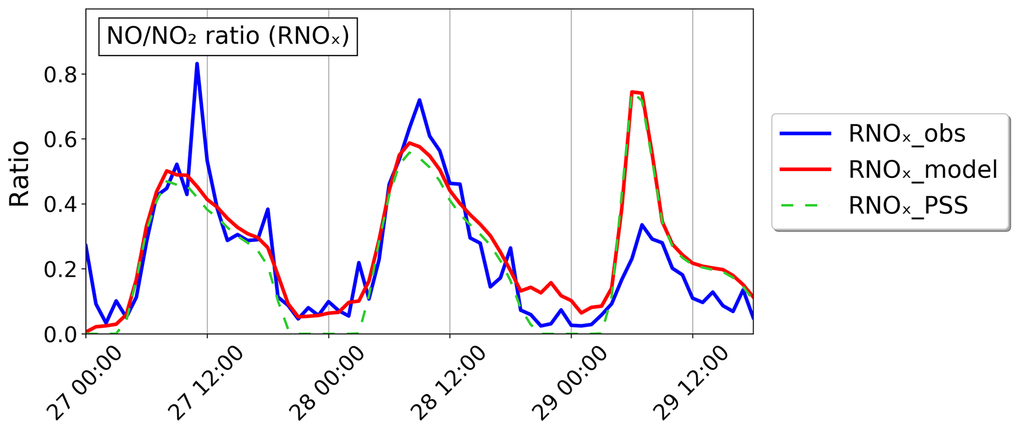
Figure 14 Observed and modeled ($\mathrm{NO}/{\mathrm{NO}}_{\mathrm{2}}$) ratio (RNOx) on 27–29 June at IRCEL-CELINE sites within the inner domain. Also shown is the ratio at photochemical steady state (RNOx_PSS), based on the concentrations and rates from the model run.

Carbon monoxide (CO), being a long-lived species, has a mostly flat evolution over the 15 d, with some peaks in the concentration indicating that the model is overestimating (22 and 25 June). The concentration of CO shown in Fig. 12 is obtained from only two stations; thus, the discrepancy between model and measurements might be due to their limited representativity or to misestimated local emission or transport patterns in the model.

The secondary pollutant O₃ is often anti-correlated with its precursor species NO_x (Han et al., 2011). For example, ozone exhibits minimum values at night, when NO₂ has its maximum. During the day, photochemistry leads to the formation of ozone and OH radicals, causing the lifetime of NO_x at a minimum. During the night, the suppression of vertical mixing leads to the accumulation of NO_x, whereas the downward transport of ozone from higher levels is reduced. The observed daily maximum ozone concentrations (of the order of 100 µg m⁻³ or about 50 ppbv – parts per billion by volume) are usually well reproduced by the model. The nighttime ozone concentrations are frequently underestimated, possibly reflecting insufficient vertical mixing. Nevertheless, the overall good agreement between model and observation indicates that the model is accurate in its representation of the photochemical processes leading to formation of ozone.

4.2.3 Diurnal cycle of surface concentrations

The average diurnal profile of the four species is shown in Fig. 15. This distinctly shows the overestimation of both NO_x compounds at night and their underestimation during the day. The NO₂ correction for interferences is highest around noon (∼ 30 % increase), when the concentration of peroxyacetyl nitrate (PAN) is maximum. PAN is a product of VOC oxidation, which occurs mostly during daytime due to the high levels of OH radicals. The early morning maximum in both NO_x compounds (at or slightly before 6:00 LT) occurs about 1 h before rush hour, and the corresponding peak in the emissions can be seen (Fig. 4). The afternoon traffic-related emission peak around 16:00 LT is not visible in the NO_x time series due to the dominant roles of the chemical sink and boundary layer development. As expected due to its longer lifetime, of the order of 50 d (Müller and Stavrakou, 2005), the diurnal variation in CO is relatively weak. Since the chemical sink is too slow to affect the diurnal shape, and since the CO emissions are maximum during daytime (as for NO_x), the nighttime maximum predicted by the model can only be due to the enhanced stability of the PBL. The observed flat diurnal profile suggests that this stability enhancement is exaggerated in the model, which is in line with the underestimation of modeled PBLH against ceilometer data (Sect. 4.1.1). As discussed above, the daytime buildup of ozone is well reproduced by the model, although there is a slight temporal shift in the peak value, for unclear reasons.

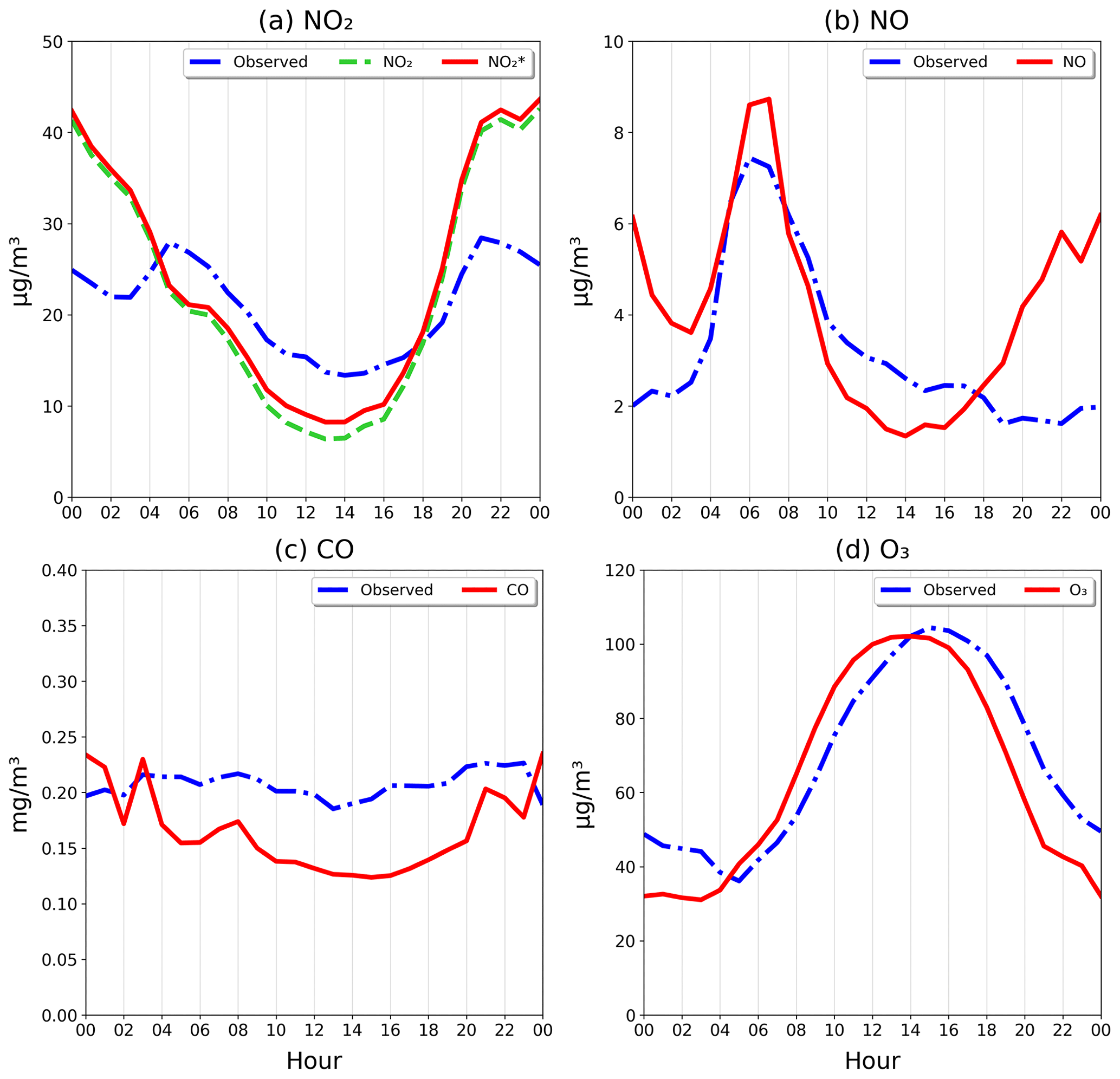
Figure 15 Average diurnal cycle of measured and modeled concentrations of (a) NO${}_{\mathrm{2}}^{*}$, (b) NO, (c) CO, and (d) O₃. Model results from the reference 15 d simulation (15–29 June) are shown. In the case of NO₂, both the interference-corrected and uncorrected model outputs are presented.

4.2.4 Improving the weekly profile of NO_x emissions based on in situ data

The relative bias (RB) of the model against daytime NO₂ data (9–17 h) calculated for each day using the (Lamsal-corrected) simulated NO${}_{\mathrm{2}}^{*}$ is shown in Fig. 16. RB is always negative and systematically higher during weekdays (−37 % on average) than during weekends (−10 %) and especially on Sundays (−4 % on 16 and 23 June). This pattern clearly suggests a misrepresentation of the weekly cycle in the emissions. The weekly shape of emissions suggested by Crippa et al. (2020) and adopted in our model simulations shows less variation between weekdays and weekends than expected, based on previous studies (e.g., Stavrakou et al., 2020; Valin et al., 2014). Indeed, spaceborne NO₂ columns (Stavrakou et al., 2020; Valin et al., 2014) were shown to be consistent with emission reductions of the order of 40 % during weekends compared to weekdays over U.S. cities. By comparison, the profiles from Crippa et al. (2020) imply a reduction of only about 15 % over the Antwerp area (Fig. 17).

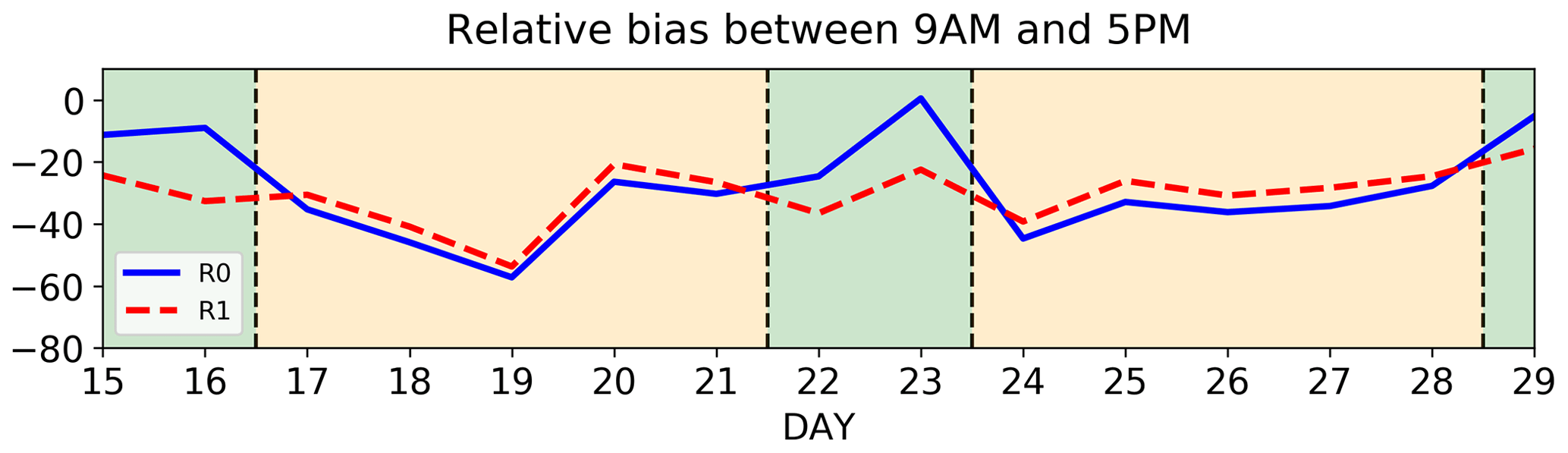
Figure 16 Average relative bias of the model against NO₂ station data, calculated for each day between 9:00 and 17:00 LT, between 15 and 29 June. The blue line shows the initial run R0, and the red dashed line shows run R1 with the updated weekly cycle of emissions (see Fig. 17). The vertical dashed lines separate the weekends (green) and weekdays (orange).

Here we use the IRCEL-CELINE measurements in combination with WRF-Chem simulations to derive a top-down emission weekly emission cycle. Following Zhu et al. (2021), a reference run and a perturbation run with a uniform percentage increase in emissions (+20 %) are conducted in order to estimate the sensitivity of NO₂ output concentrations to a change in NO_x emissions. In this way, top-down daily emissions are derived, providing an improved agreement with measurements. Those emissions are calculated using the following:

$$\begin{array}{}\text{(4)}& {\displaystyle }\mathit{\beta }={\displaystyle \frac{\mathrm{\Delta }E/E_{\mathrm{ref}}}{\mathrm{\Delta }C/C_{\mathrm{ref}}}},\text{(5)}& {\displaystyle }{E}_{\mathrm{td}}=E_{\mathrm{ref}}\times \left(\mathrm{1}+\mathit{\beta }{\displaystyle \frac{C_{\mathrm{obs}}-C_{\mathrm{ref}}}{C_{\mathrm{ref}}}}\right),\end{array}$$

where E_ref and E_td are the a priori and top-down daily emissions, respectively, β is a dimensionless scaling factor reflecting NO₂ sensitivity to emission perturbation, ΔE is the change in emission, and ΔC is the change in output concentration between the reference and perturbation runs. Here the spatial patterns of the emissions are unchanged by the inversion, and both β and the scaling factor multiplying the emissions are constant over the model domain. C_obs and C_ref are averaged concentrations over all stations during daytime (9:00–17:00 LT). Nighttime concentrations are excluded, as they are more affected by horizontal and vertical transport variability.

The β factor calculated from the two model simulations is close to 1 (in the range 0.95–1.15 over the 15 d), i.e., the concentrations are approximately proportional to the emissions. The daily emission scaling factors ($E_{\mathrm{td}}/E_{\mathrm{ref}}$) for each day of the week are shown in Fig. 17. The emissions are increased by ca. 50 % during weekdays, whereas the enhancement is much lower on Saturdays (∼ 20 %) and Sundays (∼ 10 %). The temporal variation in the emissions needed to match the in situ data is obtained by multiplying the daily averaged scaling factors by the a priori weekly profile used in the model, i.e., the Crippa profile. Upon normalization, the emission weekly cycle constrained by in situ data is obtained (dashed magenta line in Fig. 17). The normalized emissions during the weekend (ca. 0.7) are in agreement with the study of Stavrakou et al. (2020), exhibiting a lower ratio between weekend and weekday (0.6) than the profile proposed by Crippa et al. (2020) (0.87). During the rest of the week, the profile shows unexpected variations, possibly due to model errors in, for example, dynamical fields. Those likely unrealistic variations are removed in the simplified weekly profile derived in this work (black dashed line).

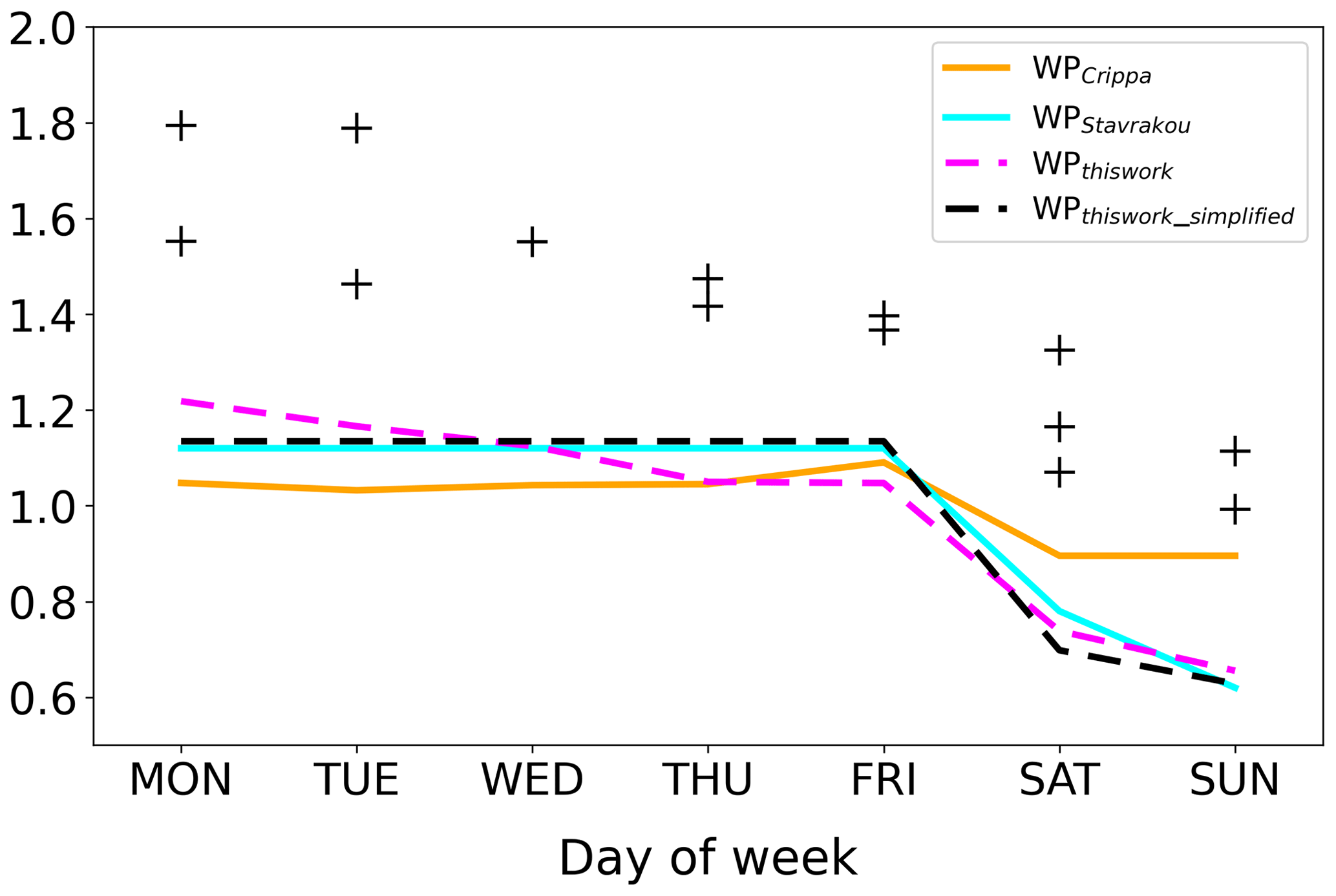
Figure 17 Normalized weekly profiles (WPs) of NO_x emissions over the Antwerp area that are (1) based on Crippa et al. (2020; orange line), (2) adopted by Stavrakou et al. (2020; blue line), and (3) derived in this work (dashed magenta line), based on the optimization of daily emissions constrained by in situ NO₂ data. Also shown is the simplified weekly profile adopted in further model calculations (see the text). The crosses represent the daily emission scaling factors needed to match the in situ data in the model. The dashed magenta line is the normalized temporal variation in emissions needed to match NO₂ data (obtained by multiplying the daily averaged scaling factors by the weekly profile from Crippa et al., 2020, followed by normalization).

Note that, besides the revised weekly profile, the top-down emissions based on station data also imply a substantial enhancement of the emissions (+43 % on average). This enhancement is likely not realistic, as it would lead to large model overestimations against remote sensing data (APEX and TROPOMI), as discussed in the next subsections. The impact of the new weekly profile is verified through an additional 15 d model simulation (R1) in which the weekly temporal profile from Crippa et al. (2020) is replaced by the new weekly cycle (WP_thiswork_simplified). As seen in Fig. 16, the R1 run generally displays a more constant relative bias of the model against NO₂ data over the 15 d time period.

4.3 Comparison with remote sensing chemical observations

4.3.1 Model evaluation against APEX data

Figure 18 compares the spatial distribution of the WRF-Chem NO₂ tropospheric column (from run R0) against the regridded APEX column measurements on 27 and 29 June. Generally, the model setup is accurate in its representation of the distribution of NO₂ over the 2 d, with well-defined plumes originating in the industrial areas northeast of the city of Antwerp. The plume orientation, namely southwest and northwest on 27 and 29 June, respectively, is dictated by the wind direction, which is about 30^∘ on 27 June and 120^∘ on 29 June (Fig. 7).

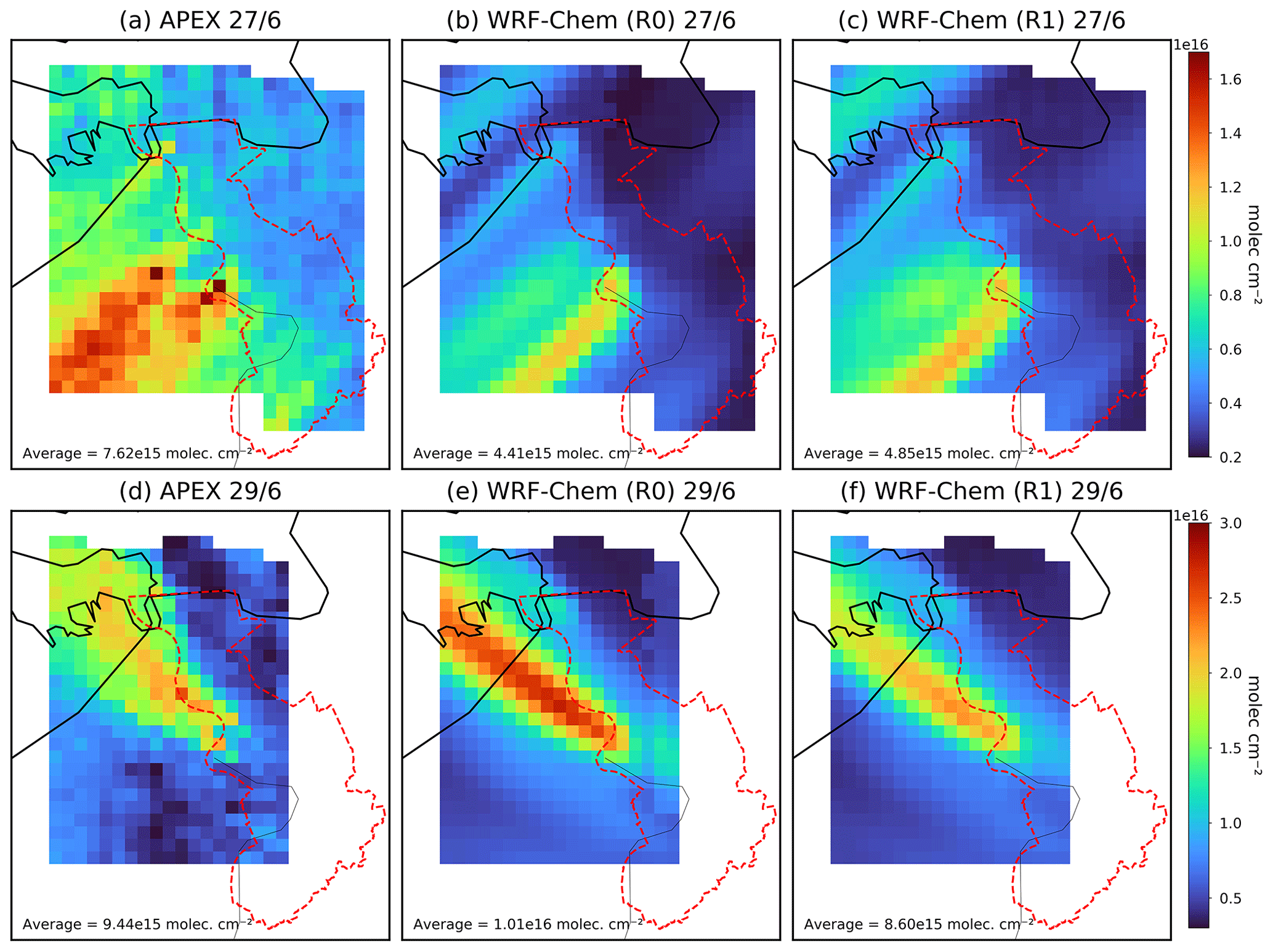
Figure 18 APEX and corresponding WRF-Chem NO₂ distribution on 27 (a–c) and 29 (d–f) June 2019. The APEX data were regridded onto the 1 × 1 km² model grid. The red dashed outline represents the region of the municipality of Antwerp. Measurements are shown in the leftmost column, while the middle and right columns display the modeled columns obtained from simulations R0 and R1. The average column value is shown in each panel.

Similar to the comparison with ground-based measurements, the modeled NO₂ in the reference run (R0) is strongly underestimated on 27 June (weekday; Thursday), while a better agreement is achieved on 29 June, which is a Saturday. On 29 June, although the regions of low emissions are well represented, the plume is more narrow and too concentrated in the WRF-Chem output, suggesting insufficient dispersion through wind transport and/or overestimation of emission sources along the axis of the plume.

The agreement with APEX data is improved by implementing the new weekly cycle constrained by IRCEL-CELINE data described in the previous section (Fig. 17). The emissions increase on Thursday (by almost 10 %) and decrease on Saturday (by ∼ 20 %) as result of this change. This improves the consistency in terms of how the model performs over the 2 d. On 29 June, the mean bias (+7 % in R0) becomes negative (−9 % in R1). The negative model bias of run R0 (−43 % on average) on 27 June remains large (−36 %). This could be partly due to the larger wind speed overestimation (by ∼ 2 m s⁻¹ on 27 June vs. ∼ 1 m s⁻¹ on 29 June; see Fig. 7) leading to excessive evacuation of the pollution plume by horizontal transport and to enhanced vertical mixing due to wind-favored turbulence.

4.3.2 Evaluation of TROPOMI NO₂ based on APEX and WRF-Chem simulation

The modeled NO₂ columns are evaluated against near-simultaneous APEX and TROPOMI measurements, whereby the model acts as an intercomparison platform to compare the two measurement techniques and develop on previous validation studies (Tack et al., 2021) to characterize biases. For a meaningful comparison, APEX data (regridded to the model resolution) and the corresponding model NO₂ columns (obtained by convolution of model profiles with the averaging kernels from either APEX or TROPOMI) are regridded to the resolution of TROPOMI. Note that, on 29 June, two TROPOMI overpasses were available for comparison. Note, however, that the second overpass (08855) had larger viewing zenith angles in the APEX area (∼ 63^∘), resulting in about twice as large pixel sizes than those of 27 June and of the first overpass on 29 June. Furthermore, the time difference between the TROPOMI and APEX measurements is larger for the second overpass of 29 June. As in Tack et al. (2021), we keep data from the first overpass (08854) for comparison only.

As seen in Fig. 19, the model correlates very well with both APEX and TROPOMI data (R>0.9), but it consistently underestimates the observed NO₂ columns on 27 June, with slopes lower than 1 for both linear regressions. The slopes are higher on 29 June, for which an excellent agreement is found between the model and TROPOMI. Interestingly, the ratio of the two slopes (model vs. APEX and model vs. TROPOMI) is similar for the 2 d (0.84 and 0.81), suggesting a moderate but consistent underestimation of TROPOMI NO₂ with respect to APEX. Note that the TROPOMI underestimation would be more pronounced without the application of averaging kernels to the model profiles (slope ratio of ∼ 0.67), as can be seen from the regressions of model columns with APEX and TROPOMI given in the Supplement (Fig. S2).

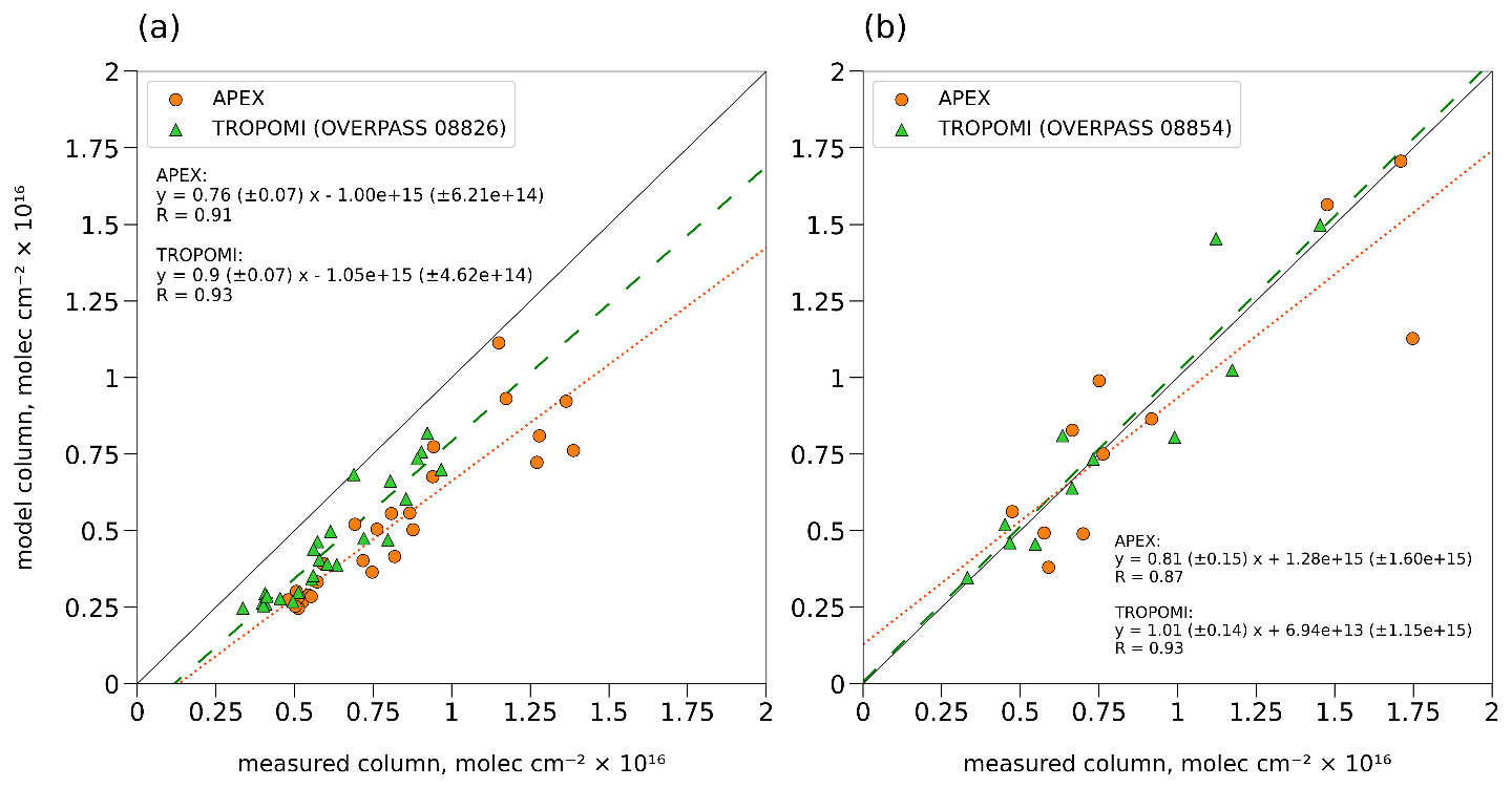
Figure 19 Scatterplots and linear regressions of modeled vs. measured columns (APEX and TROPOMI_v1.3) on (a) 27 June and (b) 29 June. Orange dots and dotted regression lines are for APEX and green triangles and lines for TROPOMI.

By combining the linear regressions of the model results against APEX and TROPOMI, a linear relationship between APEX and TROPOMI columns is derived.

$$\begin{array}{}\text{(6)}& \mathrm{APEX}=\left({\displaystyle \frac{m_{\mathrm{T}}}{m_{\mathrm{A}}}}\right)\mathrm{TROPOMI}+\left({\displaystyle \frac{c_{\mathrm{T}}-c_{\mathrm{A}}}{m_{\mathrm{A}}}}\right),\end{array}$$

where m_A and m_T are the slopes of the linear regressions between the model and APEX and TROPOMI, respectively, and c_A and c_T denote their intercepts. Taking the average of the slope and intercept obtained in this way for the 2 d, and assuming APEX to be the truth, we derive a formula intended to correct for the TROPOMI biases identified above.

This bias correction for the TROPOMI v1.3 product is given by the following:

$$\begin{array}{}\text{(7)}& C_{\mathrm{v}\mathrm{1.3}}^{\prime }=(\mathrm{1.217}\pm \mathrm{0.16})\times C_{\mathrm{v}\mathrm{1.3}}-(\mathrm{0.783}\pm \mathrm{1.3})\times {\mathrm{10}}^{\mathrm{15}},\end{array}$$

where $C_{\mathrm{v}\mathrm{1.3}}^{\prime }$ and C_v1.3 are the bias-corrected and uncorrected TROPOMI columns (molec. cm⁻²), respectively. A similar analysis was performed for the TROPOMI_PAL product (see Fig. S3 in the Supplement), leading to the following bias correction formula:

$$\begin{array}{}\text{(8)}& C_{\mathrm{PAL}}^{\prime }=(\mathrm{1.055}\pm \mathrm{0.14})\times C_{\mathrm{PAL}}-(\mathrm{0.437}\pm \mathrm{1.3})\times {\mathrm{10}}^{\mathrm{15}}.\end{array}$$

Note that the bias correction was obtained using TROPOMI data in the approximate range (4–15) × 10¹⁵ molec. cm⁻². The correction might therefore not be applicable outside of this range.

The above regressions were obtained by using the WRF-Chem model in a specific setting, namely a 15 d simulation adopting scheme P1 as PBL parameterization, with NO_x emissions and temporal variations, as described in Sects. 2.2 and 4.2.4. Since the modeled NO₂ vertical profile shapes show some dependence on the choice of PBL scheme (Fig. 11), 1 d sensitivity simulations (starting on 27 June at 00:00 UT) were conducted to estimate the impact of the PBL scheme on the regressions for the 27 June. Only schemes P1, P5, P8, P11, and P12 were tested, since the other schemes (P2, P4, P6, P9, and P10) were found to deteriorate the model performance against meteorological data and surface NO₂ measurements (Sect. 4.1 and 4.2). The regressions of the modeled columns against APEX and TROPOMI show very little dependence on the PBL scheme. For example, the regression slope from the comparison against APEX data varies by less than 1 % between the different schemes. The variance of the slopes is only slightly larger (1.5 %) for the comparison with TROPOMI, and the variance of their ratio is also very small (1.2 %). Similarly, the 15 d run and the 1 d run adopting the same PBL scheme (P1) have very similar results in comparison to APEX and TROPOMI. Finally, a 1 d sensitivity run with NO_x anthropogenic emissions enhanced by 43 % (achieving a better model agreement with APEX on 27 June and with daytime surface NO₂ data) increases the slopes of the regressions of the model vs. both APEX and TROPOMI by more than 50 % but leaves their ratio essentially unchanged (+0.5 %). These tests show that the above bias correction formulas are only very weakly dependent on the model settings.

4.3.3 Adjustment of emissions using WRF-Chem and TROPOMI data

The TROPOMI and WRF-Chem tropospheric NO₂ column distributions are compared in Fig. 20 over the model domain. To minimize the features due to transient transport effects, and to reduce the noise, the data were regridded to 0.1^∘ × 0.1^∘ resolution and averaged over the 15 d of the simulation.

Application of the bias correction to TROPOMI data, as described in Eq. (7), enhances the columns by up to 10 % (or 8 × 10¹⁴ molec. cm⁻²) over hotspots such as Paris and industrial areas around Antwerp, Rotterdam, and the northern Rhine/Ruhr region in western Germany. TROPOMI columns below 3.6 × 10¹⁵ molec. cm⁻² are decreased by the bias correction, but as discussed in the previous section, the validity of this correction is uncertain for low columns. The model succeeds in reproducing the main hotspots, although it clearly underestimates TROPOMI over Paris, Brussels, Zeebrugge (Belgian coast), and the northern part of the Ruhr Valley. The R1 model overestimates the data over the Rhine Valley and Amsterdam. The strongest model overestimation is found in a region to the west of the Rhine, located within the box labeled PP in Fig. 20. Several among the largest coal power plants in Germany (Neurath, Niederaussem, and Frimmersdorf) are located in this area (https://globalenergymonitor.org, last access: 9 January 2023). The strong hotspot north of the city of Antwerp is a special case, with an underestimation being found over the harbor of Antwerp and an overestimation across the border in the Netherlands. Generally, WRF-Chem R1 underestimates the low NO₂ columns, such as over the eastern Netherlands and Flanders, the North Sea, and northern France. The bias correction improves the model agreement with the observations in these regions, although it brings the TROPOMI columns below the WRF-Chem values over the least polluted areas in northern France, namely the Belgian Ardennes and the Eifel plateau.

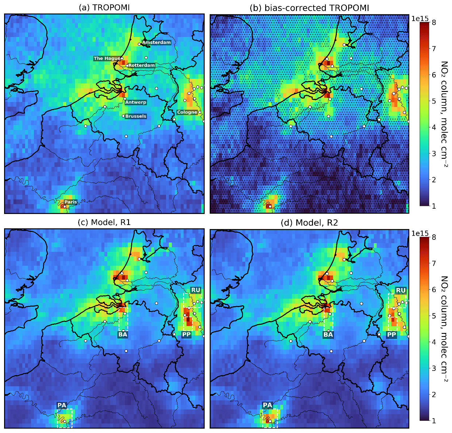
Figure 20 Spatial distribution of (a) uncorrected and (b) bias-corrected TROPOMI NO₂ columns (OFFL v1.3.1) alongside WRF-Chem simulations using (c) a priori emissions (R1) and (d) top-down emissions (R2). Model and data were regridded to 0.1^∘ × 0.1^∘ and averaged over the 15 d simulation period. The stippling in panel (b) indicates pixels for which the bias correction might be invalid (TROPOMI <4 × 10¹⁵ molec. cm⁻²). White circles represent cities with >200 000 population. The dashed white boxes represent four regions of interest, namely Paris (PA), Brussels–Antwerp (BA), the Ruhr area (RU), and a cluster of powerplants in western Germany (PP).

Many factors might contribute to the differences between the model and (bias-corrected) TROPOMI, including errors in the model transport and chemistry and in the bias correction. However, a major source of error lies in the estimation of the emissions. Here we apply a crude method to correct the spatial distribution of emissions in the model, by making the assumption that emission errors are the leading reason for the differences with TROPOMI. The method uses equations similar to those used to amend the weekly cycle (Eqs. 4 and 5), where C_ref and C_obs denote 15 d averaged WRF-Chem and (bias-corrected) tropospheric NO₂ columns, respectively. A reference run and a perturbed run with 20 % increased NO_x emissions are used to update the emissions. This emission update is not considered reliable below the validity range of the bias correction, all the more because low NO₂ columns are also disproportionately affected by the long-range transport from more polluted areas. By contrast, the NO₂ hotspots are primarily due to local emissions. Note, however, that even the hotspots are affected by wind transport, which is likely the main source of error in this optimization of emissions. To limit such errors, the emission correction is not kept when the modeled column shows a weak sensitivity to emission changes, i.e., when the β factor (Eq. 4) is significantly higher than unity (more specifically β>1.45). High values of β (Fig. S4) are found away from the major emission regions and near the borders of the model domain due to the influence of lateral boundary conditions. Over polluted areas, β is generally close to, or even lower than, unity. Lower-than-one values of β indicate that chemical feedbacks amplify the effect of emission changes on the concentrations. Indeed, in high NO_x areas, increasing NO_x emissions depletes the OH radical through the NO₂+ OH reaction (Lelieveld et al., 2016), and this reaction is the main sink of NO_x. Over low NO_x areas, NO₂+ OH is negligible as OH radicals sink, and NO_x emission increases lead to enhanced O₃ and OH levels, mainly due to the HO₂+ NO reaction which converts HO₂ to OH and produces ozone. This explains the higher values of β over more remote areas (such as the Belgian Ardennes), as the NO_x emission increase leads to shorter NO_x lifetimes.

Figure S4 shows the difference between the observed and modeled tropospheric NO₂ column for the reference run (R1) and for a run using the emissions adjusted as described above (R2). Note that the R1 simulation already performs quite well, since the average model bias over polluted areas (TROPOMI >4 × 10¹⁵ molec. cm⁻²) is only −6 % in simulation R1 (−4 % in run R2). The emission adjustment (Fig. S5b) leads to improvements in the match between model and observation, which is particularly evident in the northern Rhine and Ruhr regions, where both overestimations in the southwestern part (between Cologne and Krefeld) and underestimations in the northern part have now decreased. Emission increases over the Paris and Brussels–Antwerp areas also reduce the overall model underestimation in these regions. To summarize, the negative biases over the Paris area (box labeled “PA” in Fig. 20), Brussels–Antwerp (BA) and the Ruhr Valley (RU) decrease, respectively, from −33 %, −13 % and −14 % in simulation R1 to −5 %, −6 % and −9 % in simulation R2 using top-down emissions. These improvements are realized by increasing the emissions by 39 % (PA), 20 % (BA), and 13 % (RU) on average over each region. At the same time, the model overestimation around the large German power plants (PP) decreases from 19 % to 8 % thanks to emission decreases averaging −19 % in this region. In other areas, such as Rotterdam and The Hague, the top-down emissions fail to improve the agreement, however. This is likely due to transport effects, since the column in 1 pixel is dependent on emissions in many neighboring pixels, and the pattern of model biases is particularly heterogeneous around Rotterdam and The Hague and other regions.

5 Discussion and conclusions

Several validation campaigns for the TROPOMI NO₂ product (version 1.3) have been conducted in areas, mostly in mid-latitude areas in the vicinity of strong emission sources, similar to the region simulated in this study. Methods include comparison with ground-based differential optical absorption spectroscopy (DOAS) measurements and with airborne spectral imagers (e.g., APEX). Those studies generally report either the relative bias of TROPOMI NO₂ with respect to the correlative measurements or, more frequently, the slope (s) and intercept (i) of regressions of the type $C=i+sC$', where C denotes the TROPOMI column and C' the independent measurements. The relationship derived between APEX and TROPOMI v1.3 (Eq. 7) in this work can be expressed similarly, with s=0.82, and i=6.4 × 10¹⁴ molec. cm⁻². The relative bias of TROPOMI v1.3 is calculated to be about −10 % for columns in the range (6–12) × 10¹⁵ molec. cm⁻². The TROPOMI_PAL product achieves even lower biases in this range (between −2 and +2 %), with s=0.95, and i=4.1 × 10¹⁴ molec. cm⁻².

Based on comparisons with multi-axis DOAS (MAX-DOAS) measurements at 19 sites worldwide, Verhoelst et al. (2021) inferred negative biases in TROPOMI tropospheric NO₂ columns, estimated at −37 % in slightly polluted conditions (2 × 10¹⁵ molec. cm⁻²) and −51 % in highly polluted areas (12 × 10¹⁵ molec. cm⁻²). Those biases are much larger than those obtained in this work (about −10 %). A first reason for this discrepancy might be the different spatial representativeness of ground-based and spaceborne or airborne data, especially in urbanized/industrial areas. In addition, as pointed out by Verhoelst et al. (2021), large errors in TROPOMI tropospheric columns are due to shortcomings in the a priori NO₂ profile used in the TROPOMI product algorithm. A comparison between satellite and independent measurements can be improved by replacing the standard a priori vertical profile of TROPOMI NO₂, obtained from the TM5-MP model, with a new profile obtained either from a higher-resolution model or from measurements, when available. This highlights the importance of accounting for the difference in a priori profile and vertical sensitivity between TROPOMI and the independent instrument. This was realized in this work (Sect. 4.3.2) by applying averaging kernels from TROPOMI and APEX to the model concentrations when calculating the corresponding model columns. Without the averaging kernel application, the slope s of the relationship between APEX and TROPOMI (calculated from the regressions of Fig. S2) would be 0.67, and the resulting TROPOMI bias would be estimated at −19 % for a column of 8 × 10¹⁵ molec. cm⁻².

This work uses the validation data described and used by Tack et al. (2021) to evaluate TROPOMI. Based on a direct comparison of APEX and TROPOMI, Tack et al. (2021) determined TROPOMI NO₂ biases of −21 % and −15 % for the two flights over Antwerp. This is consistent with our comparisons performed when ignoring averaging kernels (Fig. S2). Substitution of the TM5-MP a priori profiles with the high-resolution profiles from CAMS (at 0.1^∘ × 0.1^∘ resolution) in the TROPOMI dataset was found, by Tack et al. (2021), to improve the comparison considerably, e.g., by lowering the average bias to about −2 %. The slope of the regression between TROPOMI and APEX was also improved from ∼ 0.7 with the original product to 0.83–0.94 with the CAMS-modified dataset. Those values compare well with the slope obtained here (0.82).

Tropospheric NO₂ columns were evaluated over the New York area using airborne and ground-based Pandora observations (Judd et al., 2020). The regression slope of the standard TROPOMI NO₂ product against airborne columns was 0.68, which increased to 0.77 when correcting for the a priori vertical profile of the NO₂ product obtained from the North American Model–Community Multiscale Air Quality (NAMCMAQ) modeling system. The slopes for the comparison with ground-based Pandora data were 0.8 and 0.82 for the TM5 and NAMCMAQ products, respectively, which are very similar to the slope derived in this study. Similar results were found by Griffin et al. (2019) using ground-based Pandora column data and airborne concentration measurements above the Canadian oil sands. Biases ranging between −15 % and −30 % for the original TROPOMI dataset were reduced to between 0 % and −25 % when using modified air mass factors based on high-resolution model profiles and improved surface reflectivity and snow identification.

Pandora measurements at urban and suburban sites in the Greater Toronto Area showed slopes of 0.70–0.77 for the standard TROPOMI NO₂ product and between 0.76 and 0.85 when updating the a priori NO₂ profile to a higher-resolution profile shape and updating the albedo and snow flags (Zhao et al., 2020), which is also consistent with our findings. In contrast, measurements by the same group at a rural site (Egbert) indicated overestimations of TROPOMI NO₂, relative to the Pandora columns, of about 10 %–15 % for columns of the order of 4 × 10¹⁵ molec. cm⁻².

Dimitropoulou et al. (2020) and Chan et al. (2020) evaluated TROPOMI NO₂ data in Uccle (near Brussels) and Munich, respectively, using 2-D MAX-DOAS instruments. Significant negative biases of the original TROPOMI product were found, amounting to −30 % or more at both sites. Upon replacement of the a priori vertical NO₂ profiles of the TROPOMI algorithm with the MAX-DOAS profiles, however, these negative biases are reduced in Munich (to ca. −20 %) and disappear almost completely in Uccle.

To conclude, the moderate TROPOMI v1.3 underestimation (−10 %) and slope of regression against APEX data (0.82) obtained in this study are well in line with previous validation studies in polluted conditions. The agreement between TROPOMI and correlative tropospheric NO₂ measurements shows systematic improvement when the NO₂ vertical profile utilized in the air mass factor calculation of the satellite product is replaced by higher-quality profiles obtained from either measurements (e.g., MAX-DOAS) or a high-resolution model. Alternatively, the difference in vertical sensitivity and a priori profiles of the two instruments (when available) can be dealt with through the use of averaging kernels, as in the present study using the WRF-Chem model as intercomparison platform, or more directly by applying the formalism of Rodgers and Connor (2003), as was done recently for validating TROPOMI formaldehyde (HCHO) data using Fourier transform infrared spectroscopy (FTIR) measurements (Vigouroux et al., 2020).

Nevertheless, the comparison of spaceborne columns with ground-based optical measurements is made difficult by the high heterogeneity of NO₂ abundances, especially near emission hotspots. This is illustrated by the dependence of comparison statistics on spatial coincidence criteria, as seen in many studies (e.g., Zhao et al., 2020; Dimitropoulou et al., 2020; Chan et al., 2020). To a large degree, this representativeness issue disappears when evaluating TROPOMI against APEX data, due to their very fine resolution (70 × 120 m²) and large number ensuring high spatial coverage of TROPOMI pixels. Furthermore, adopting a fine-resolution model as an intercomparison platform together with careful model sampling strategy allows us to take care of co-location differences and differences in vertical sensitivity and a priori profiles. The validation results from this work and from previous studies provide strong evidence that TROPOMI v1.3 NO₂ columns are only moderately underestimated under polluted conditions (typically −10 % for columns >4 × 10¹⁵ molec. cm⁻²) when a priori profile shape differences are properly accounted for. More work is needed to characterize the performance of TROPOMI in less polluted conditions, although there is evidence of a slight overestimation of low NO₂ columns. The overestimation of the high columns essentially disappears in the recently released TROPOMI_PAL product, at least in the column range considered here.

Although the model compares generally well with meteorological observations, it struggles to accurately represent near-surface wind speed, which is in line with previous studies indicating wind speed overestimations of the order of 1 m s⁻¹ near the surface over Europe (Tuccella et al., 2012). This discrepancy might be partly due to underestimated surface roughness length in WRF-Chem over forests and urban areas, as noted by Shen et al. (2020). This might impact boundary layer mixing and horizontal transport processes and adds further uncertainties to comparisons with ground-based chemical observations. The diurnal profile of NO₂ is too pronounced in the current model setup, showing too high maxima during the night and a consistent underestimation during the day. This could be in part due to a misrepresentation of the diurnal cycle of emissions from Crippa et al. (2020), or to issues with the model transport, including wind speed overestimation and insufficient vertical mixing during the night, leading to a buildup of NO₂. In addition, chemistry represents an additional source of uncertainty. The concentrations of OH, the main reaction partner of NO_x during daytime, are strongly impacted by short-lived NMVOC emissions, which could be underestimated. In addition, VOC emissions also affect the formation of PAN and organic nitrates, thereby influencing the NO_x sink and the interference impacting the NO₂ measurement (Eq. 2). Further work should aim at evaluating those emissions and their chemical representation in WRF-Chem, for example, through comparisons with TROPOMI HCHO column data.

Nevertheless, the model is capable of suitably reproducing the major features of NO₂ column distribution over both simulation domains, matching the shape and location of plumes seen from aircraft measurements, and locating hotspots as seen from TROPOMI.

Although inconsistencies between the modeled and observed NO₂ columns are partly due to errors in the model transport and chemistry, the distribution of the model–data differences allows for the evaluation of bottom-up emission inventories. In the regions where high-resolution emissions are available, i.e., over Flanders and the Netherlands, the comparison indicates slight overestimations of bottom-up emissions e.g., over Amsterdam and slight underestimations over Antwerp. Determining which sectors are responsible for the overestimation will require further investigation. Over the rest of the simulation domain, where EMEP was used as a priori, significant underestimations are found in the region of Paris, where emission increases of about 40 % are required to match the observations. The regions of Brussels and Düsseldorf also appear to have localized underestimations in the reference runs. The EMEP emissions from a cluster of powerplants in the Rhine region (PP in Fig. 20) appear to be overestimated by more than 20 %. Upon further inspection, it appears plausible that the location of the very large Neurath power plant (51.038^∘ N, 6.611^∘ E) has been misplaced in the EMEP inventory. This would indeed explain the mislocation of the strongest NO₂ column hotspot from the model distribution, which is one 0.1^∘ pixel to the west of Neurath. These results are preliminary, however, and more work will be needed to refine the proposed adjustments to the inventories based on satellite observations. These efforts will eventually help in obtaining more accurate emission estimates and ultimately provide support to mitigation policies.