the Creative Commons Attribution 4.0 License.
the Creative Commons Attribution 4.0 License.
 | 18 Aug 2023
Dynamic Meteorology-induced Emissions Coupler (MetEmis) development in the Community Multiscale Air Quality (CMAQ): CMAQ-MetEmis
Bok H. Baek
Carlie Coats
Siqi Ma
Chi-Tsan Wang
Yunyao Li
Jia Xing
Daniel Tong
Soontae Kim
Jung-Hun Woo
There have been consistent efforts to improve the spatiotemporal representations of biogenic/anthropogenic emission sources for photochemical transport modeling for better accuracy of local/regional air quality forecasts. While biogenic emissions, bi-directional NH3 from fertilizer applications, and point source plume rise are dynamically coupled in the Community Multiscale Air Quality (CMAQ) “inline”, there are still known meteorology-induced emissions sectors (e.g., on-road mobile sources, residential heating, and livestock waste), with little or no accounting for the meteorological impacts in the currently operational chemical and aerosol forecasts, but they are represented with static, not weather-aware annual or monthly county total emissions and standard monthly, weekly, or daily temporal allocation profiles to disaggregate them on finer timescales for the hourly air quality forecasts. It often results in poor forecasting performance due to the poor spatiotemporal representations of precursor pollutants during high ozone and PM2.5 episodes. The main focus of this study is to develop a dynamic inline coupler within the CMAQ system for the on-road mobile emission sector that requires significant computational resources in the current modeling application. To improve their accuracy and spatiotemporal representations, we developed the inline coupler module called CMAQ-MetEmis (for meteorology-induced emission sources within CMAQ version 5.3.2 modeling system). It can dynamically estimate meteorology-induced hourly gridded on-road mobile emissions within the CMAQ, using simulated meteorology without any computational burden to the CMAQ modeling system.
To understand the impacts of meteorology-driven on-road mobile emissions on local air quality, the CMAQ is applied over the continental U.S. for 2 months (January and July 2019) for two emissions scenarios, namely (a) “static” on-road vehicle emissions based on static temporal profiles and (b) inline CMAQ-MetEmis on-road vehicle emissions. Overall, the CMAQ-MetEmis coupler allows us to dynamically simulate on-road vehicle emissions from the MOtor Vehicle Emission Simulator (MOVES) on-road emission model for CMAQ, with a better spatiotemporal representation based on the simulated meteorology inputs when compared to the static scenario. The domain total of daily volatile organic compound (VOC) emissions from the inline scenario shows that the largest impacts are from the local meteorology, which is approximately 10 % lower than the ones from the static scenario. In particular, the major difference in the VOC estimates was shown over the California region. These local meteorology impacts on the on-road vehicle emissions via CMAQ-MetEmis revealed an improvement in the hourly NO2, daily maximum ozone, and daily average PM2.5 patterns, with a higher agreement and correlation with daily ground observations.
- Article
(10714 KB) - Full-text XML
- BibTeX
- EndNote


Since the industrial revolution, chemical pollutants in the atmosphere have impacted human society due to their adverse health effects. The primary gases and particles directly emitted from their emission sources are chemically transformed into secondary pollutants through complex chemical reactions under various local meteorological conditions. Over the last 3 decades, sophisticated multiscale chemical transport models (CTMs) have been developed to predict the concentrations of primary and secondary chemicals in the lower atmosphere and actively used for air quality regulatory planning applications, in addition to air quality forecasting for the general public health (Wong et al., 2012; Byun and Schere, 2006; Dennis et al., 2010; Rao et al., 2011; Hogrefe et al., 2001). The CTM simulation results strongly rely on two major inputs, namely meteorology and emissions, thus requiring accurate estimation of both to simulate the transport, chemical transformation, and removal of the pollutants. Depending on their chemical reactivity and gravitational behaviors, some pollutants can be chemically transformed and travel a long distance from their source of origin, while some are deposited near their release locations.
To accurately predict regional and global chemicals in the future, spatially and temporally resolved meteorology and emissions are critical and are required to be rapidly updated based on the aerosol direct/indirect meteorology impacts within a fully coupled air quality modeling system. There have been considerable efforts made in the meteorology prediction enhancements being actively conducted (Jacob and Winner, 2009; Grell and Baklanov, 2011; Fiore et al., 2012; Wong et al., 2012). However, there have been only limited “inline” emissions modeling enhancements made to the CTM system for which emissions from meteorologically driven air pollutant emission processes are dynamically coupled within the regional/global CTM modeling system, rather than being estimated a priori and statically provided as model inputs based on “offline” spatial and temporal allocations. Simulating emissions inline is especially crucial for real-time air quality forecasting (Tong et al., 2012). In particular, the system of the National Oceanic and Atmospheric Administration (NOAA) National Air Quality Forecast Capability (NAQFC) allows us to induce the influences of the forecast meteorology on emissions from key sources, such as stationary power plants, vegetation, fertilizer applications, such as mineral dust (Knippertz and Todd, 2012), sea salt (Foltescu et al., 2005; Pierce and Adams, 2006), biogenic volatile organic compounds (BVOCs; Lathière et al., 2005; Chen et al., 2018), and biomass burning events (Grell et al., 2011; Pavlovic et al., 2016). Despite these scientific advancements and model improvements, true process-based interaction between the local meteorology and meteorology-induced anthropogenic pollutant emissions from on-road vehicles, livestock waste, and residential heating remain incomplete or overlooked (Pouliot, 2005; Tong et al., 2012).
The mobile/transportation sector is one of the most important anthropogenic emissions sectors in metropolitan regions, where most of the high ozone and PM2.5 concentration episodes often occur (Andrade et al., 2017; Kumar et al., 2018; Perugu, 2019). It is also known that the performance and emissions of mobile engines are sensitive to local weather conditions, such as ambient temperature and humidity (Lindhjem et al., 2004; Iodice and Senatore, 2014; Choi et al., 2010; Mellios et al., 2019). This incomplete fuel combustion can occur under cold ambient temperatures and high humidity, leading to higher emissions being emitted. The effect of humidity on internal combustion engines, including spark-ignition engines (gasoline, liquefied petroleum gas or LPG, and natural gas) and compression ignition or diesel engines, has been known for many years, with evidence indicating that higher humidity results in lower NOx emissions (Lindhjem et al., 2004; U.S. EPA, 2015). Additional emissions also come from the energy use of air conditioning at higher ambient temperatures. These meteorological impacts can be accounted for using state-of-the-art mobile emissions models such as the U.S. EPA's MOtor Vehicle Emission Simulator (MOVES) version 3.0 (U.S. EPA, 2021a). However, it lacks transparency with respect to the air pollutant emission algorithms, including key parameters such as emission factors. Furthermore, it requires significant computational resources to generate these high-quality spatiotemporal emissions from on-road vehicles (Li et al., 2016; Xu et al., 2016; Liu et al., 2019; Perugu, 2019). To generate the offline, weather-aware, on-road mobile emissions outside the current Community Multiscale Air Quality (CMAQ), MOVES has been integrated with the Sparse Matrix Operator Kernel Emissions (SMOKE) modeling system, called the SMOKE-MOVES integration tool (Baek et al., 2010), by processing (reading, storing, and/or accessing) MOVES emission factor (EF) datasets. However, it demands significant computational time and memory in the SMOKE-MOVES integration approach due to the high traffic of the input/output (I/O) data, which largely prohibits its usage in real-time air quality forecasting. As an example, the latest version of SMOKE version 4.8.1 can require approximately 1.9 computing hours with up to 20 GB RAM to generate 25 h CMAQ-ready gridded hourly emissions over the continental U.S. (CONUS) modeling domain (12 km × 12 km grid size) offline.
To enable the indirect/direct feedback effects of aerosols and local meteorology in an air quality modeling system without any computational bottleneck, we have developed an inline meteorology-induced emissions coupler module within the U.S. EPA's CMAQ modeling system (called the Meteorology-induced Emissions Coupler or CMAQ-MetEmis) to dynamically model the complex MOVES on-road mobile emissions inline. To address the shortcomings (computational time and memory requirements) in the current slow offline SMOKE-MOVES integration approach, we first re-restructured the SMOKE-MOVES integration tool by storing the ambient temperature-specific gridded hourly emissions into a pseudolayer structure for easy and fast access. Each pseudolayer holds the gridded chemically speciated hourly emissions from an incremental temperature bin (e.g., 10 and 20 ∘F (−12.2 and −6.67 ∘C) and so on). The CMAQ-MetEmis coupler was developed to estimate the gridded hourly emissions with a simple linear interpolation between two temperature bins' gridded hourly emissions, based on a simulated hourly ambient temperature. With an instance interpolation calculation approach, the new inline CMAQ-MetEmis approach significantly enhances the computational efficiency compared to the existing offline SMOKE-MOVES approach without losing any accuracy of the emission estimates. We also evaluate the performance of the CMAQ-MetEmis coupler module in CMAQ, which includes their computational performance, the feasibility of CMAQ-MetEmis implementation as a forecasting application, and the responses of O3 and PM2.5 to the meteorological impacts on anthropogenic emissions.
NOAA has developed the NAQFC, operated by the National Weather Service (NWS), in partnership with the U.S. EPA, using the state-of-the-art air quality modeling system, CMAQ, to forecast the concentrations of O3 and PM2.5 over the contiguous continental U.S. (CONUS), Alaska, and Hawaii (Tong et al., 2015; Lee et al., 2017; Tang et al., 2017). Unlike weather forecasting, air quality forecasting requires full atmospheric chemistry, along with the physical state and tendency of the weather in the near future. Accurate prediction of meteorology and emissions for CMAQ plays a critical role in the accuracy of 48 and 72 h air quality forecasting. The current NOAA/NWS operational requirements specify that the post-processing of the simulated/forecasted meteorological data, emission data, and air quality chemistry model simulations be completed in a reasonable time frame to meet the air quality forecasting time constraints. Since the processing of the meteorological data and the execution of the air quality chemistry model are the most time-consuming parts of the CMAQ, minimizing the processing time of the emissions is desirable. A typical emission-processing over the CONUS national domain for 1 d may take up to 2 h on a single central processing unit (CPU; Intel Xeon Gold 6240R with 2.4 GHz) using SMOKE and other emission post-processing tools. To expedite the operational forecasting streamlines, non-meteorologically dependent emissions are generally processed in advance (Tong et al., 2015). Only the meteorologically induced emission sources are processed during the air quality forecasting simulation runs. So then, the accuracy of the emission processing can be maintained, and the forecast can be completed within the required time constraints.
2.1 Meteorology-induced mobile emissions
Mobile emissions from the on-road and off-network (e.g., vehicle start-up, running exhaust, brake–tire wear, hot soak, and extended idling) are sensitive to temperature and humidity due to various factors, including (1) cold engine starts that enhance emissions at lower ambient temperatures due to incomplete fuel combustion, (2) evaporative losses of volatile organic compounds (VOCs) due to expansion and contraction caused by ambient diurnal temperature variations, (3) enhanced running emissions at higher ambient temperatures, (4) atmospheric moisture suppression of high combustion temperatures that lower nitrogen oxide emissions at higher humidity, and (5) indirect increased emissions from air conditioning at higher ambient temperatures (Choi et al., 2010; Iodice and Senatore, 2014; Lindhjem et al., 2004; Mellios et al., 2019; U.S. EPA, 2015). McDonald et al. (2018) found that NOx emissions from the National Emissions Inventory (NEI) estimated from the U.S. EPA's MOVES are underestimated, leading to a failure regarding the prediction of high ozone days (8 h max ozone >70 ppb; McDonald et al., 2018).
The dependency of mobile emissions on local meteorology can vary by vehicle type (light duty, heavy duty, truck and bus), fuel type (gasoline, diesel, hybrid, and electric), road type (interstate, freeway, and local roads), process (vehicle start-up, running exhaust, brake–tire wear, hot soak, and extended idling), vehicle speed for on-road vehicles, and hour of the day for off-network vehicles, as well as by pollutants such as CO, NOX, SO2, NH3, VOCs, and particulate matter (PM). Figure 1 shows the dependency of the MOVES emission factors of CO, NOx, VOCs, and PM2.5 from gasoline-fueled vehicles on ambient temperature from the on-road and off-network vehicles, respectively. All pollutant emissions vary with the temperature, particularly under lower speeds. The CO, VOCs, and NOx emissions increase with temperature, while the opposite relationship is suggested between PM2.5 emissions and temperature, implying the complexity of meteorology impacts on different pollutant emissions. For off-network emissions from gasoline-fueled vehicles, CO, NOx, and PM2.5 show negative correlations with temperature, while the VOCs exhibit a nonlinear response to the temperature variation. The largest meteorology dependency occurs in the daytime when emissions are the greatest. A further, detailed meteorology dependency of MOVES emission factors on local meteorology can be found in Choi et al. (2010).
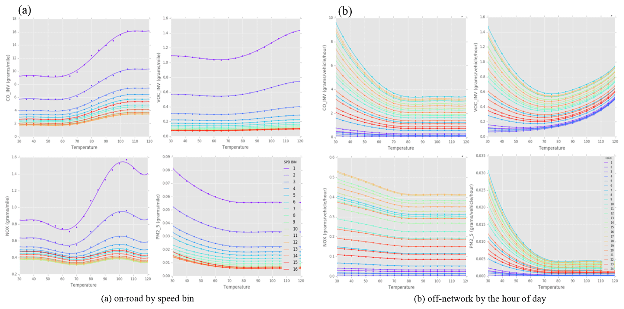
Figure 1Meteorology dependency of CO, VOCs, NOx, and PM2.5 emissions from gasoline-fueled light-duty vehicles by average speed bin (a) and the off-network vehicles by the hour of day (b).
2.2 SMOKE-MOVES integration tool
In 2010, the U.S. EPA introduced the process-based on-road mobile emissions model, MOVES, which is a state-of-the-art MySQL database-driven software for calculating bottom-up vehicular emissions from on-road and off-network vehicles. Depending on its application, MOVES can generate on-road mobile emissions in two different modes. The inventory mode can generate the county-level monthly total emissions inventory, while the emission rates mode can generate the complex emission rates, which are a function of local meteorological variables, such as ambient temperature and humidity. They play a key role in the emissions from vehicles on the roads. The county total emissions inventory in a unit of tonnes per month or tonnes per year from the inventory mode can be directly processed through the SMOKE modeling system with the static temporal allocation profiles (e.g., weekly and diurnal profiles) to generate the CMAQ-ready gridded hourly emissions. However, the emission rates mode can generate the complex emission factors for SMOKE to dynamically estimate the temporally and spatially enhanced on-road mobile emissions with the simulated meteorology inputs. Unlike the inventory mode, the emission rates mode MOVES runs can take up to 30 h to generate the detailed emission factors for each county. MOVES can generate the emission factors for off-network emission processes (e.g., parked engine off, engine start-up, idling, and fuel vapor venting), which are hour-dependent due to vehicle activity assumptions built into the MOVES model; the emission rate in a unit of grams per mile per hour depends on both the hours of the day and the temperature. It can also generate detailed emission factors for on-road emission processes (e.g., running exhaust, crankcase running exhaust, brake wear, tire wear, and on-road evaporative emissions); however, these factors do not depend on the hour but are expressed in grams per mile.
MOVES is approved for use in any official state implementation plan (SIP) submitted to the U.S. EPA and for conformity emissions inventory development outside of California. Furthermore, it can be used to estimate on-road vehicle emissions for a variety of different purposes, namely to evaluate the national and local emissions trends, to compare different emission scenarios, to analyze the benefits of mobile source control strategies, and to provide inputs for air quality modeling. Although MOVES estimates of mobile emissions include the dependence on vehicle activities and simulated hourly meteorology, its computational requirements are prohibitive in real-time air quality forecasting applications. The dynamic offline SMOKE-MOVES tool was developed by integrating MOVES emission factor (EF) outputs with the SMOKE modeling system prior to the CMAQ simulation (Baek, 2010), with the objective of improving the accuracy of mobile emissions for air quality modeling applications. The tool can dynamically estimate hourly mobile emissions based on vehicle activity inventories (i.e., miles traveled, population, and operating hours), MOVES EFs (a function of vehicle type, road type, and local meteorology), simulated hourly ambient temperatures, and humidity. It first estimates spatially and temporally averaged county-level hourly meteorological inputs (temperatures and humidity). It then prepares driver and post-processing scripts to set up and run MOVES to generate county-specific MOVES EF lookup tables (LUT) and to sort them by average vehicle speed, ambient temperature, humidity, operating hours, day of the week, and/or hour of the day. Finally, the tool runs a SMOKE program called Movesmrg, which is designed to process the MOVES EF LUTs to estimate the air quality model-ready gridded hourly emissions with simulated hourly meteorology (Fig. 2a).
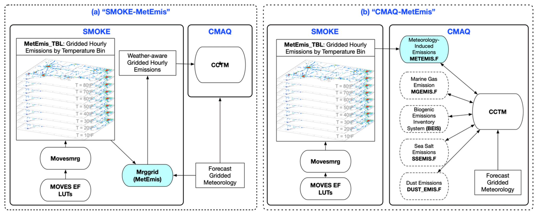
Figure 2Meteorology-induced Emissions Coupler module (MetEmis) with the air quality modeling systems of (a) SMOKE-MetEmis, and (b) CMAQ-MetEmis.
Based on the latest 2017 National Emissions Inventory (NEI) Emissions Modeling Platform (EMP; U.S. EPA, 2021b), the SMOKE-MOVES integration tool processes over 668 county-level MOVES EF LUT files (334 files per season), ranging from 60 up to 150 MB, to model over 3100 counties in their modeling domain (e.g., 12 km × 12 km grid over the continental U.S.), which requires significant computational resources such as memory, computing time (>1.9 computing hours for 25 h processing), and storage space. The SMOKE-MOVES integration step for the on-road mobile emission sector requires the most computational time, and it is not feasible for us to implement it into the current NAQFC forecasting system, which will significantly delay its processing time due to its computational resource requirement. Details on its computational requirements will be described in a later section.
2.3 MetEmis dynamic coupler
Although the current offline SMOKE-MOVES integration tool can estimate weather-aware on-road mobile emissions for CTMs using their local meteorology, it is not fully coupled with CTMs to dynamically provide aerosol direct/indirect feedback to climate and meteorology and to enhance the air quality forecast modeling applications in seasonal-to-sub seasonal predictions due to its slow computation process.
Table 1The required computational memory and time in the SMOKE modeling system. Note that RPD is the RatePerDistance, RPV is the RatePerVehicle, and RPH is the RatePerHour.
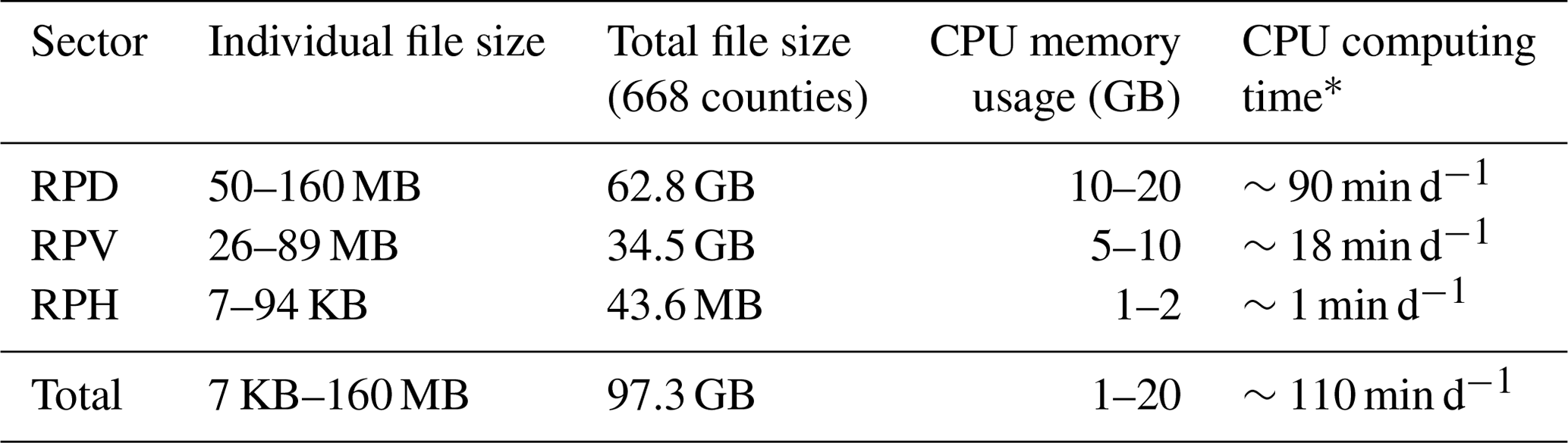
* The specification of the CPU is Intel Xeon Gold 6240R with 2.4 GHz.
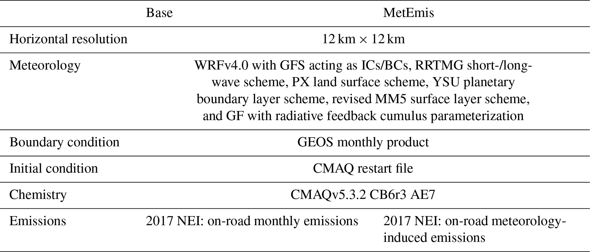
Table 2CMAQ modeling domain and configurations. Note that GFS is for Global Forecast System, ICs is for the initial conditions, BCs is for the boundary conditions, RRTMG is for rapid radiative transfer model for global climate models, YSU is for Yonsei University, MM5 is for the Fifth-Generation Penn State/NCAR Mesoscale Model, PX is for Pleim–Xiu, GF is for Grell–Freitas, GEOS is for Goddard Earth Observing System, and NEI is for National Emissions Inventory.
In this study, we developed the Meteorology-induced Emissions Coupler module (MetEmis) within the CMAQ modeling system to enhance the current NAQFC with the weather-aware emissions modeling capability without any computational burden to the system. Pouliot (2005) indicated that the main obstacle to implementing weather-aware mobile emissions into air quality simulation is a significant computational resource requirement, especially for air quality forecasting applications. To address these potential shortcomings (computational time and memory requirements) without compromising on any accuracy compared to the current offline SMOKE-MOVES integration tool, we first implemented a new, optional feature in the Movesmrg program in the SMOKE v5.0 modeling system to generate the temperature-specific pregridded hourly emissions called MetEmis_TBL that holds them in the pseudolayer structure for easy and fast access for a later weather-aware emissions coupler (Fig. 2). Each pseudolayer holds the pregridded hourly emissions based on predefined temperature bins (e.g., 5, 10, 15 ∘C, and so on). Thus, the single MetEmis_TBL file that holds both fuel months (January – winter; July – summer) can replace the entire MOVES EF LUT files for SMOKE and CMAQ modeling system to generate the CTM-ready, weather-aware mobile emissions.
There are two ways to process the MetEmis_TBL emissions output file from SMOKE (Movesmrg) to develop weather-aware emissions more easily and faster, namely (a) SMOKE-MetEmis and (b) CMAQ-MetEmis. SMOKE-MetEmis is an offline approach, which is practically the same as the SMOKE-MOVES integration, other than processing the MetEmis_TBL emissions file instead of over 668 ASCII-formatted MOVES EF LUT files from MOVES. Both SMOKE-MetEmis and SMOKE-MOVES approaches generate identical offline gridded hourly emissions prior to the CMAQ simulations, but SMOKE-MetEmis is significantly faster (Fig. 2a). The updated Mrggrid utility tool from SMOKE v5.0 will first read and process the MetEmis_TBL emissions file with the simulated forecast meteorology prior to the CMAQ simulations. However, the CMAQ-MetEmis is a true inline approach based on the CMAQ version 5.3.2, with a new dynamic emission coupler module called MetEmis that can generate weather-aware emissions with MetEmis_TBL within the CMAQ simulations (Fig. 2b). This means that it can be dynamically coupled to estimate weather-aware emissions inline without any computational burdens under the CMAQ-parallelized simulations. Details of the computational enhancements are discussed in the next section.
2.4 MetEmis computational efficiency
While estimating meteorologically induced on-road mobile emissions using local meteorology accurately provides the emissions to CTMs, the current offline SMOKE-MOVES integration tool approach has faced many challenges, such as computational burdens, the data portability and distribution issues due to the size of the data files, and computationally expensive I/O data processing. Accurately generating the on-road mobile emissions for the continental U.S. using MOVES on-road emission model requires a significant number of computational resources, in addition to processing time. It takes approximately 12 computing hours to generate one county MOVES EF LUT table per month using MOVES (Baek et al., 2010). Simulating over 3100 counties in the continental U.S. (CONUS) for 12 calendar months (>37 400 MOVES simulations) will require a tremendous number of computational resources and a large amount of time. Thus, U.S. EPA has adopted the representative county approach to reduce the number of counties and the number of modeling months. Each representative county was classified according to its state, altitude (high or low), fuel region, the presence of inspection and maintenance programs, the mean light-duty vehicle age, and the fraction of ramps. A total of 296 representative counties for CONUS and 38 for Alaska, Hawaii, Puerto Rico, and the U.S. Virgin Islands was selected (U.S. EPA, 2022). Each representative county holds 2 fuel months to represent all 12 calendar months.
To generate 1 d (25 h time steps) CMAQ-ready gridded hourly emissions, SMOKE needs to read and process 334 MOVES EF LUT in addition to many other SMOKE-ancillary input files such as vehicle mileage traveled (VMT) activity, temporal profiles, chemical speciation profiles, spatial surrogates, and so on. The most computational resources are consumed during the I/O (input and output) processes of the number of data files while complex datasets are being processed. Table 1 shows the estimated computational resources and time for each on-road mobile sector (e.g., RatePerDistance, RPD, RatePerVehicle, RPV, and RatePerHour, RPH). Among the mobile sectors, RPD and RPV are the slowest sectors being processed in the SMOKE modeling system. Each mobile sector contains a total of 668 MOVES LUT files (334 counties × 2 fuel months), and a total of 2004 (=668 × 3 sectors) MOVES LUT files are processed to generate the mobile sector-specific CMAQ-ready gridded hourly emissions.
Based on the latest 2017 NEI EMP, CMAQ-ready gridded hourly emissions in our modeling domain (e.g., 12 × 12 km grid over the continental U.S.) require approximately 1.9 h d−1 (RPD of 90 min, RPV of 18 min, and RPH of 1 min) to generate the complete set of on-road mobile daily emissions, including the RPD, RPV, and RPH modes. It may require over 638.5 h (∼ 29 d) of computational time to generate CONUS gridded hourly emissions for 365 d. While the CMAQ-MetEmis inline approach (Fig. 2b) does not require much computational processing time since, the I/O of the NetCDF or input/output applications programming interface (I/O API) binary format MetEmis_TBL input file in the CMAQ modeling system is instantaneous. There was less than 1 min d−1 of CMAQ computational time with 96 CPUs of parallel processing.
The latest version of SMOKE can generate a single MetEmis_TBL output file as an option. It can hold the 25 temperature bins of gridded hourly emissions for 334 representative counties for 1 fuel month from 0 to 125 ∘F (51.67 ∘C) temperature (25 bins with 5 ∘F (−15 ∘C) increments). Correction equations for humidity are applied to estimate the grid cell hour adjustment factors for NOx emissions by fuel type (U.S. EPA, 1997). Because on-road sectors (e.g., RPD, RPV, and RPH) share the same linear interpolation to estimate the emission factors between two temperature bins from the MOVES LUT files, the sector-specific MetEmis_TBL files can be merged and represent all sectors, with one-time interpolation through SMOKE-MetEmis and CMAQ-MetEmis modules.
Thus, the merged MetEmis_TBL file can represent the entire USA, with 334 representative county-specific MOVES LUT files per fuel month and with 25 temperature bins. The size of MOVES_TBL is approximately 16 GB, which is significantly smaller than the size for all 2004 MOVES LUT files for all RPD, RPV, and RPH sectors, which is ∼ 97.3 GB (62.8 GB + 34.5 GB + 48 MB; Table 1). Approximately 6 h were required to generate the MetEmis_TBL file once with SMOKE per fuel month, prior to the CMAQ-MetEmis simulations. This MetEmis_TBL can hold more than a single fuel month with the increased file size and replace the entire 2004 MOVES LUT files (∼ 97.3 GB) for both fuel months (e.g., January – winter; July – summer) with the single MetEmis_TBL file (∼ 16 GB). The final merged MetEmis_TBL file is portable and can be a direct input for the CMAQ-MetEmis coupler in the CMAQ modeling system.
The CMAQ air quality modeling runs are configured close to the current operational NAQFC, including the spatial coverage, emission inputs, and chemical transport model. It contains three major components, namely meteorology, emissions, and chemical transport models. The Weather Research and Forecasting (WRF) model version 4.2.1 (Skamarock et al., 2021) is used to generate hourly meteorological fields to drive emissions and air quality modeling. The WRF model was configured with the Morrison two-moment microphysics scheme, a rapid radiative transfer model for global climate models (RRTMG) long- and short-wave radiation scheme, a Yonsei University (YSU) planetary boundary layer (PBL) scheme, a Pleim–Xiu land surface model, the revised MM5 (Jimenez) surface layer scheme, and Grell–Freitas (GF), with a radiative feedback cumulus parameterization option. The emissions input was provided using a hybrid emission modeling system that utilized the SMOKE model version 4.8.1 (Baek and Seppanen, 2021) to process anthropogenic emissions and a suite of emission models to estimate emissions from intermittent and/or meteorology-dependent sources. Anthropogenic emissions were taken from the U.S. EPA 2017 NEI EMP. The CMAQ model (version 5.3.2) ingests the emissions and meteorology to predict the spatiotemporal variations in the atmospheric pollutants (such as O3, NO2, and particulate matter), using a revised carbon bond 6 gas-phase mechanism and the aerosol model 7 (AE7) mechanism (CB6r3_AE7_AQ; Byun and Schere, 2006; Luecken et al., 2019).
Table 3Statistical metrics between observed and simulated O3, NO2, and PM2.5 in January and July 2019 over the contiguous United States. Note that CORR is the correlation coefficient, RMSE is the root mean square error, NMB is the normalized mean bias, and NME is the normalized mean error.
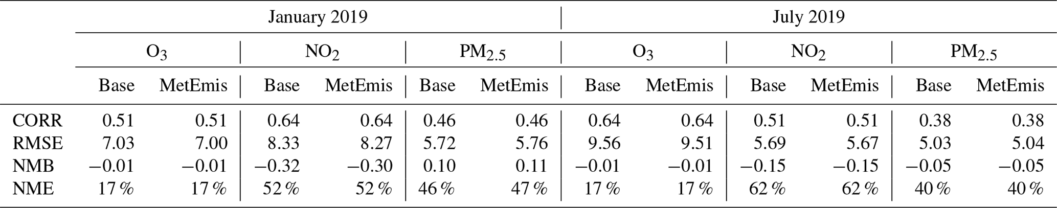
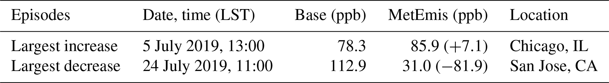
Table 4The largest differences in the ozone episodes in July 2019 over the USA.
The meteorological, emissions, and air quality models have 12 × 12 km horizontal resolution over the contiguous United States, with full 35 sigma layers vertically and the domain top at 50 hPa. The WRF model was driven by the forecast fields of the Global Forecast System (GFS) version 4 products, with a horizontal resolution of 0.25∘ × 0.25∘ (available every 6 h), and was reinitialized every 24 h to be consistent with its operational task.
To understand the impacts of meteorology-induced on-road emissions on the local air quality, we conducted two CMAQ simulation scenarios (Base and MetEmis). All simulations were conducted for 2 months, January and July, in the year 2019. We initiated our CMAQ simulations based on the default CMAQ background concentration profiles. The first 3 d of the CMAQ simulation were used as a spin-up modeling period to eliminate the influence of the initial condition (Chen et al., 2021; Lv et al., 2018; Tong and Mauzerall, 2006). The configurations and simulations are listed in Table 2.
-
A Base scenario, which is a static offline approach based (not weather-aware) on gridded hourly emissions based on the county total emissions with static temporal profiles (monthly, weekly, month to day, and hourly).
-
A MetEmis scenario, which is a dynamic inline approach based on weather-aware gridded hourly emissions dynamically estimated with simulated meteorology using the inline CMAQ-MetEmis approach.
The monthly total emissions inventories used in the Base scenario are based on the MOVES inventory mode simulation, with monthly average ambient temperature and humidity, while the MOVES emission rates mode simulation was used for the MetEmis scenarios with the simulated hourly temperature and humidity. In order to evaluate the impact of the MetEmis approach, we analyze the response of NOx, VOCs, NH3, and PM2.5 emissions to the dynamic inline MetEmis coupler approach. The evaluation of the CMAQ-MetEmis air quality modeling system was performed by the comparison of the simulated ambient concentrations of NO2, O3, and PM2.5 with the observations for which most of the meteorology-induced emissions are impacted by the meteorology compared to the static offline approach (i.e., Base). Note that both Base and MetEmis on-road mobile emissions are from the 2017 NEI EMP package.
3.1 Weather-aware mobile emissions
The huge computational burden of the traditional offline SMOKE-MOVES approach prohibits its usage in providing real-time estimates of mobile emissions, which might be significantly driven by weather changes, resulting in considerable uncertainties in predicting emissions and air quality. The spatial monthly total difference plots of VOCs and NOx between Base and MetEmis from Fig. 3 clearly show that most of the emission differences caused by local meteorology occur from major interstate roads and metropolitan cities (e.g., New York, Detroit, Chicago, Los Angeles, Phoenix, and Atlanta), where on-road mobile emissions contribute the most. In particular, the largest differences in VOCs occurred over the Californian region in July 2019, probably because the original temporal profiles assumed in Base are not suitable to represent the real condition influenced by the weather. The January and July VOC emissions from the Base scenario were higher by over 8 % and 20 % than the ones from the MetEmis scenarios, respectively, indicating that current NAQFC-ready on-road mobile emissions (not weather-aware) are significantly over-representing the VOC emissions compared to the weather-aware VOCs dynamically estimated by MetEmis.
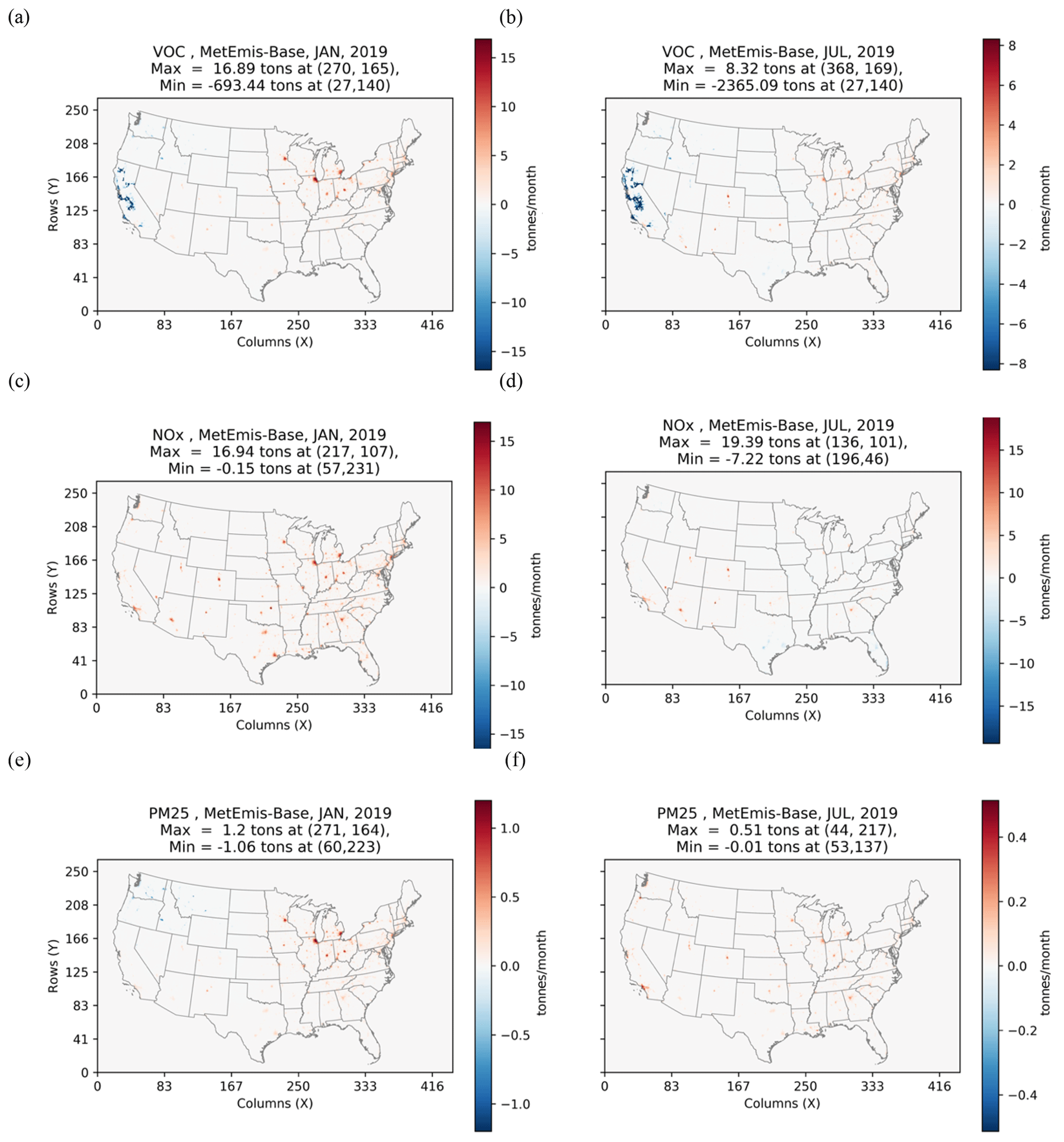
Figure 3Spatial comparison of monthly total emissions of VOCs, NO, and PM2.5. The colors indicate that MetEmis is larger (red) or smaller (blue) than Base for (a) VOCs in January, (b) VOCs in July, (c) NOX in January, (d) NOx in July, (e) PM2.5 in January, and (f) PM2.5 in July.
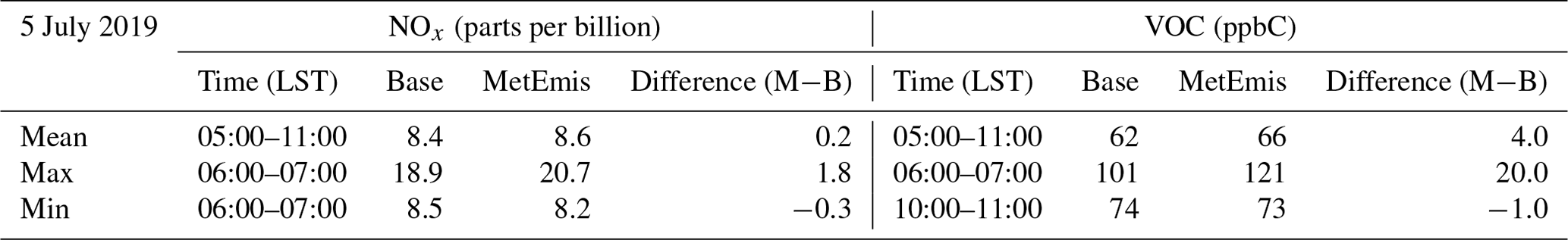
Table 5Summary of precursor (NOx and VOC) concentrations on the morning before the largest ozone increase episode at 14:00 LST on 5 July 2019 over Chicago, IL. Note that ppbC is parts per billion of carbon, M is for MetEmis, and B is for Base.
Unlike the Base approach, the MetEmis approach estimates hourly emissions by multiplying the estimated hourly vehicle mileage traveled (VMT) in the unit of miles per hour with the inventory pollutant emission rates (unit of grams per mile), which are a function of local meteorology (e.g., ambient temperature and humidity). The MetEmis emissions can enhance their spatiotemporal representations of on-road mobile sources. However, the hourly VMT activity data are estimated using the same temporal profiles used in the Base hourly emissions. Thus, both on-road emissions follow similar weekly and daily patterns, with some hourly variations based on local meteorological conditions. As presented in Fig. 4, which compares the hourly domain total TOGs (total organic gases), NOx, and PM2.5 emissions between the Base and the MetEmis approach, the statically estimated Base hourly emissions (colored blue) clearly show the repeated weekly patterns within the same month due to the usage of the static weekly temporal profiles, while the MetEmis (colored in red) display irregular hourly patterns due to the impacts of the local hourly meteorology.
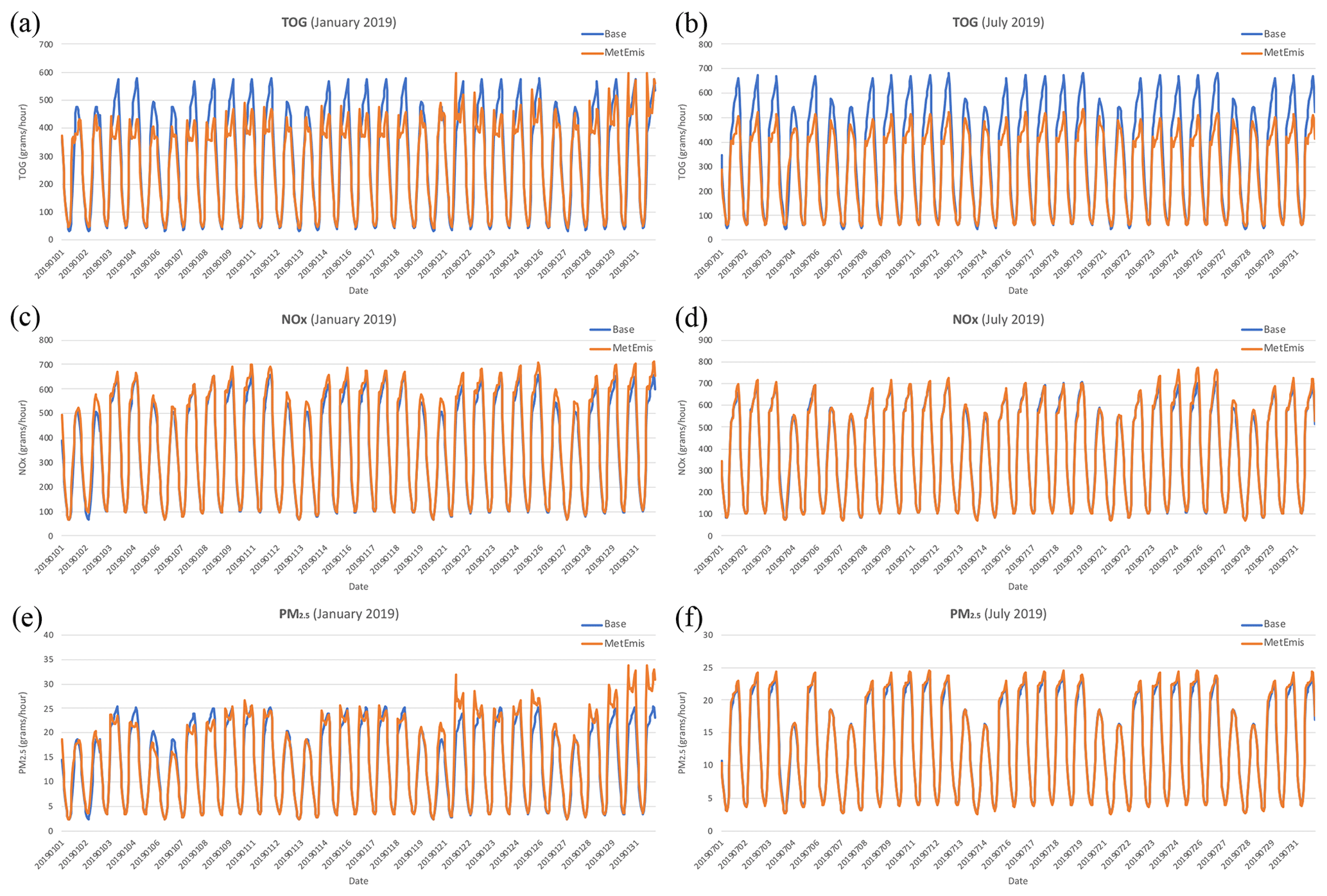
Figure 4Temporal comparisons of daily domain total emissions of (a) total organic gas (TOG) in January, (b) TOG in July, (c) NOX in January, (d) NOx in July,(e) PM2.5 in January, and (f) PM2.5 in July from the Base (blue line) and MetEmis scenarios (red line).
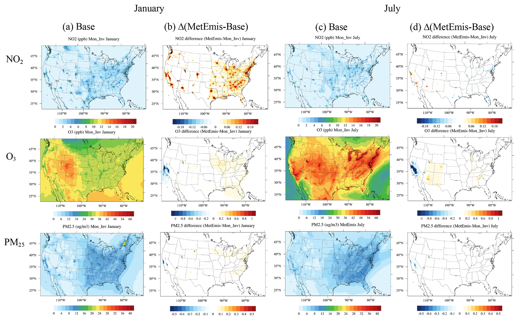
Figure 5Spatial distribution of NO2, O3, and PM2.5 concentrations and difference figures. (a) January's averaged concentrations from the Base scenario, (b) the differences between Base and MetEmis scenarios in January, (c) July's averaged concentrations from the Base scenario, and (d) the differences between Base and MetEmis scenarios in July.
Due to the influence of local meteorology (i.e., ambient temperatures and humidity), the on-road running exhaust/evaporative emissions, and the off-network evaporative emissions show a moderate decrease in TOG and a slight increase in NOx (>4 % increase) over the entire domain due to low ambient and humidity condition during the winter season (January), according to MetEmis estimates. The most important enhancement in the MetEmis approach is allowing modelers to simulate NAQFC-ready weather-aware on-road mobile emissions. More importantly, the daily differences are also noticeable in the MetEmis approach within 1 month, as higher TOGs and PM2.5 are shown in late January due to the increased temperature, while the Base approach failed to predict such a variation. Such spatiotemporal enhancements of on-road mobile emissions predicted by MetEmis, especially near metropolitan regions, would benefit the NAQFC. As stated, these on-road mobile emissions from two scenarios are based on the MOVES simulations designed for the 2017 NEI EMP.
3.2 Weather-aware mobile emissions impacts on CTM simulations
3.2.1 Domain-level evaluations
This study investigated the response of NO2, O3,, and PM2.5 to the meteorology-induced mobile emission changes by simulating air quality under two scenarios (Base and MetEmis). The sensitivity of air pollutant concentrations to these meteorology-induced emission sources was performed and analyzed in this section.
Table 6Statistics of largest ozone decrease episode (24 July 2019) over San Jose, CA.

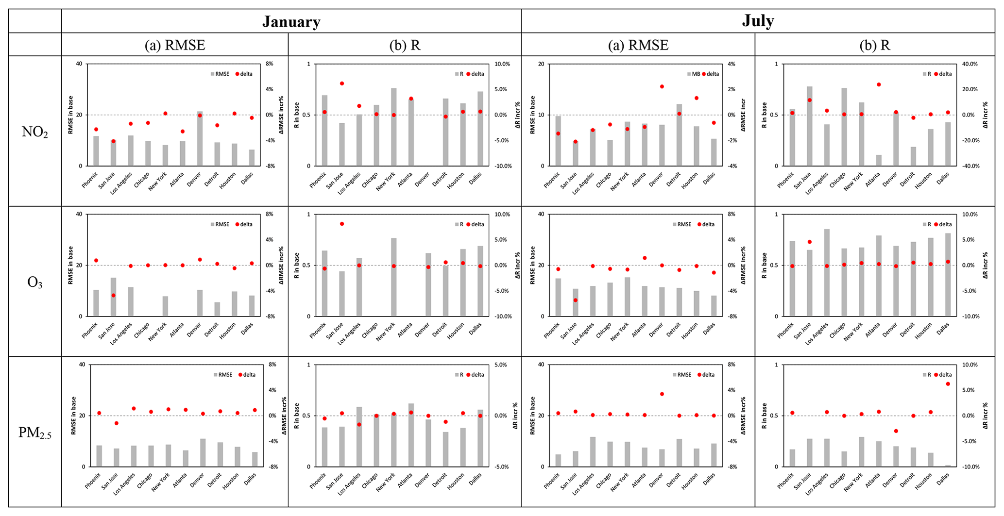
Figure 6Comparison of model performance in simulating NO2, O3, and PM2.5 concentrations between Base and MetEmis scenarios. The columns show the different model evaluation metrics in January (a and b) and July (a and b). The rows present different species, including NO2, O3, and PM2.5. RMSE is the root mean square error, and R is the correlation coefficient. Delta is (MetEmis − Base)Base; when ΔR>0 and ΔRMSE <0, indicate the improvement in MetEmis. The R of NO2 in January in Denver is −0.002, which increased to 0.008 with MetEmis. Observed O3 data are missing for Chicago and Atlanta in January.
The monthly statistical modeling evaluation metrics for these two simulations (Base and MetEmis) over the CONUS domain are provided in Table 3. The correlation coefficient (CORR) of O3 is 0.51 for both simulations, and they have the same normalized mean bias and errors (NMB and NME), while the root mean square error (RMSE) of Base (7.03 ppb) is slightly higher than that of MetEmis (7 ppb). The simulated NO2 shows the best correlations (0.64) among these three pollutants in January; however, its RMSE, NMB, and NME are the largest. The PM2.5 simulation did not reproduce the variability very well with a lower CORR of 0.46, but it presents the best RMSE and moderate NMB/NME. In July, the CORRs of O3 improved from 0.51 to 0.64, while the RMSEs are also increasing because of intense concentration in summer. NO2 and PM2.5 have the opposite pattern of O3, with decreased CORR (0.51 and 0.38, respectively) and improved biases and errors, except for the NME of NO2. Over the entire modeling domain, both simulations show quite similar modeling performances against the observations, with the difference generally below 1 %. This is mostly attributable to the spatial pattern of the emissions being primarily concentrated in urban areas. The largest impacts of MetEmis emissions are shown over metropolitan cities where mobile emissions play a critical role in the local air quality.
Figure 5 shows the monthly average NO2, O3, and PM2.5 concentrations from the Base scenario and the monthly average difference between the Base and MetEmis scenarios in July 2019. The spatial distributions of simulated NO2 present a close pattern with those of the NOx emissions in both months, demonstrating the effect of local NOx emissions on the NO2 activities. The NO2 concentration in July is lower than in January and is caused by the stronger NO2 photolysis and ventilation. In January, the NO2 simulated by MetEmis showed a higher concentration over the domain, with more than 0.2 ppb (parts per billion) larger over urban areas because of the increased NOx emissions after adjustment. In comparison, the monthly simulated NO2 concentrations with and without emission adjustment are much closer in July; the emission adjustment makes the concentration increase in the east, while a decrease is seen in the west. Compared to NO2, the secondary O3 and PM2.5 formation chemical reactions involve complex nonlinear processes under various meteorological conditions and precursor emissions. Despite their complexity, there are strong correlations between their nonlinear responses and precursor emission changes.
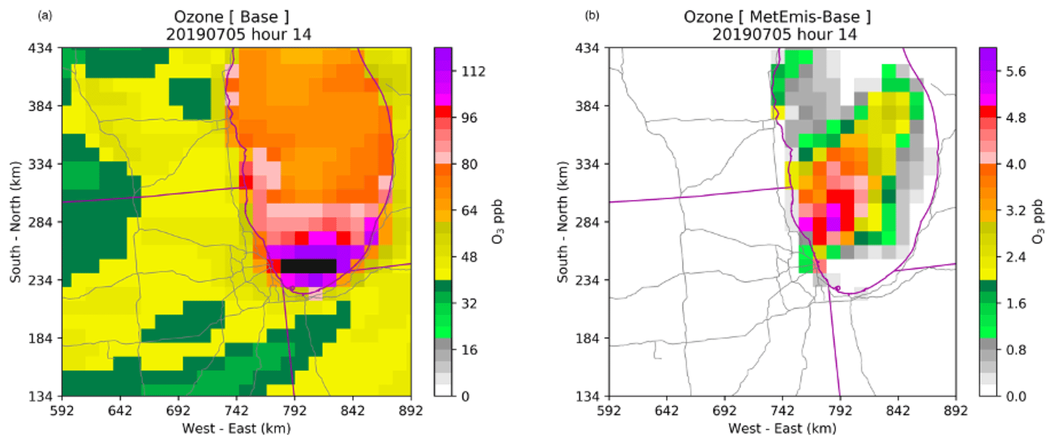
Figure 7Base hourly ozone (ppb) (a) and the hourly ozone difference (MetEmis − Base) (b) at 14:00 LST on 5 July 2019. Black coloring indicates the concentration above the color scale maximum (120 ppb).
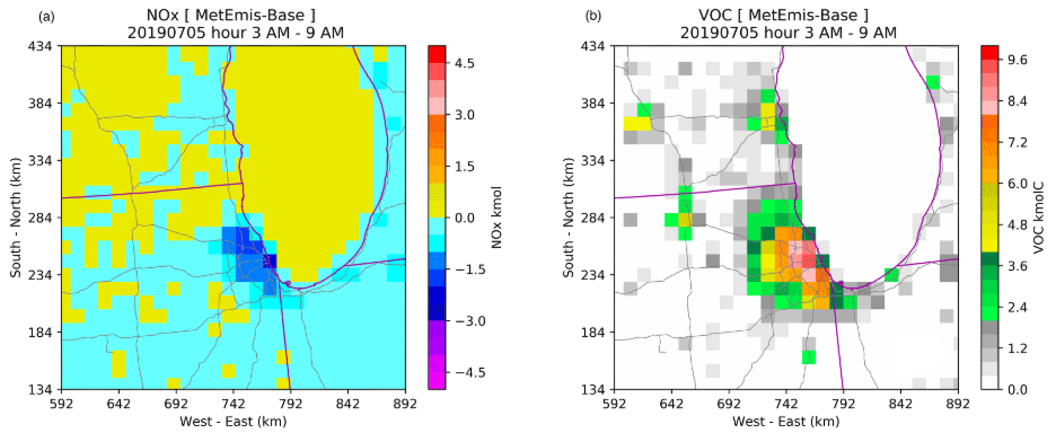
Figure 8Spatial differences in NOx (a) and VOC (b) emissions in the early morning (03:00–09:00 LST) on 5 July 2019.
3.2.2 City-level evaluation
The O3 concentration is generally below 36 ppb in most areas in January because of the cold weather and weak photolysis process, while it presents a high concentration over the midwestern USA, which is caused by the higher altitude over the Rocky Mountains area. The O3 significantly increases in July, with an average concentration of 43.9, which is 10 ppb larger than that in January. In July, the northeastern USA becomes the hot spot zone as the local anthropogenic emissions and pollution transport are strong. Meanwhile, the O3 is also concentrated over water, such as the Great Lakes and northeastern coastal areas. Most of the ozone increase occurred around the surrounding regions of metropolitan cities like Chicago, IL, Atlanta, GA, Denver, CO, and Phoenix, AZ, where both NOx and VOC emissions slightly increased during July 2019 (Fig. 3). However, the San Jose, CA, area showed a significant decrease in ozone during the summer of 2019 due to the higher VOC estimations from NEI (Base) compared to the ones from the MetEmis scenario (Fig. 3).
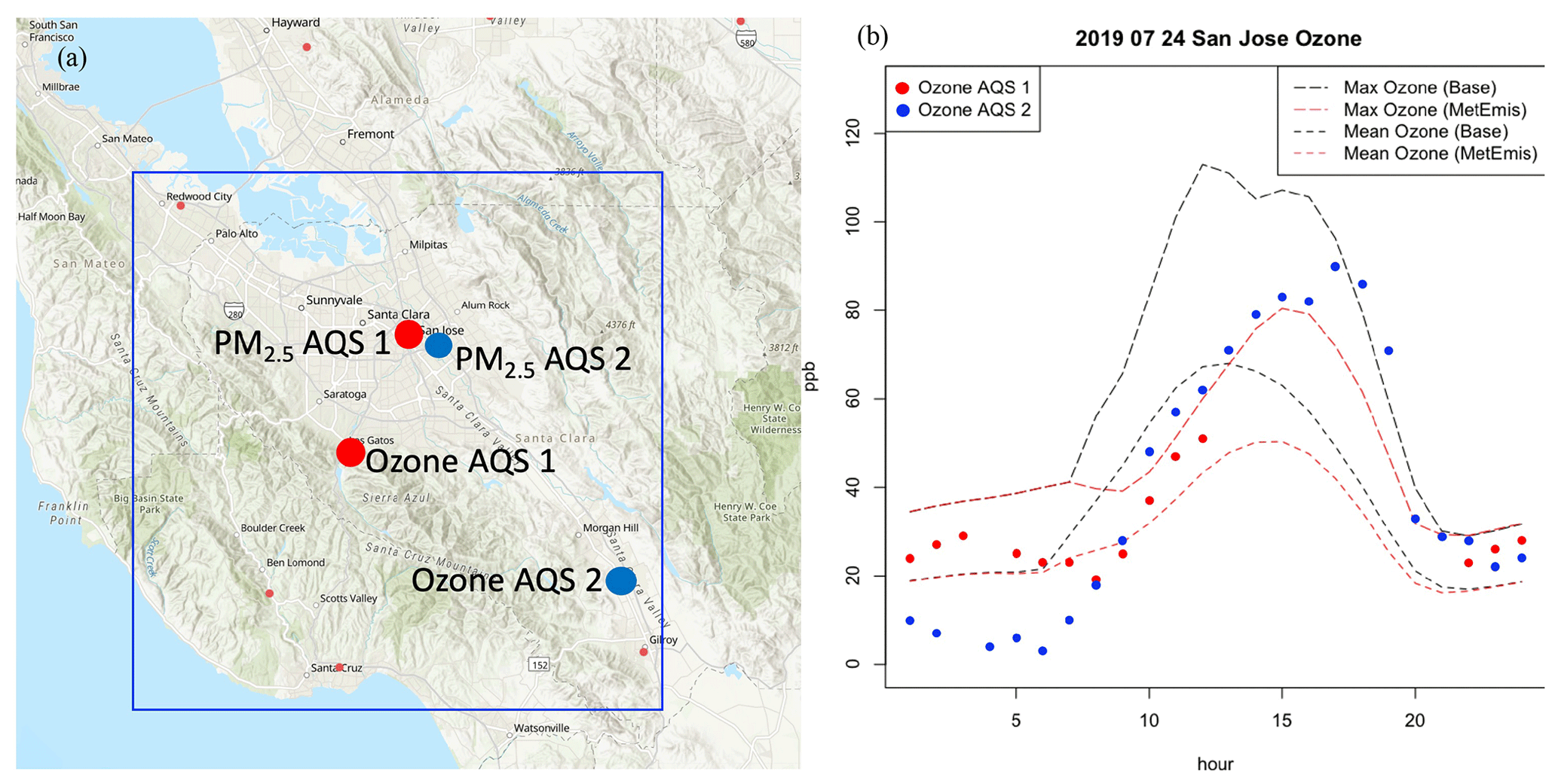
Figure 9(a) U.S. EPA's Air Quality System (AQS) ozone and PM2.5 monitoring locations and (b) diurnal variation in the ozone (maximum and mean) on 24 July 2022 over San Jose, CA. The base map layer of this figure was made by Esri (Esri et al., 2013).
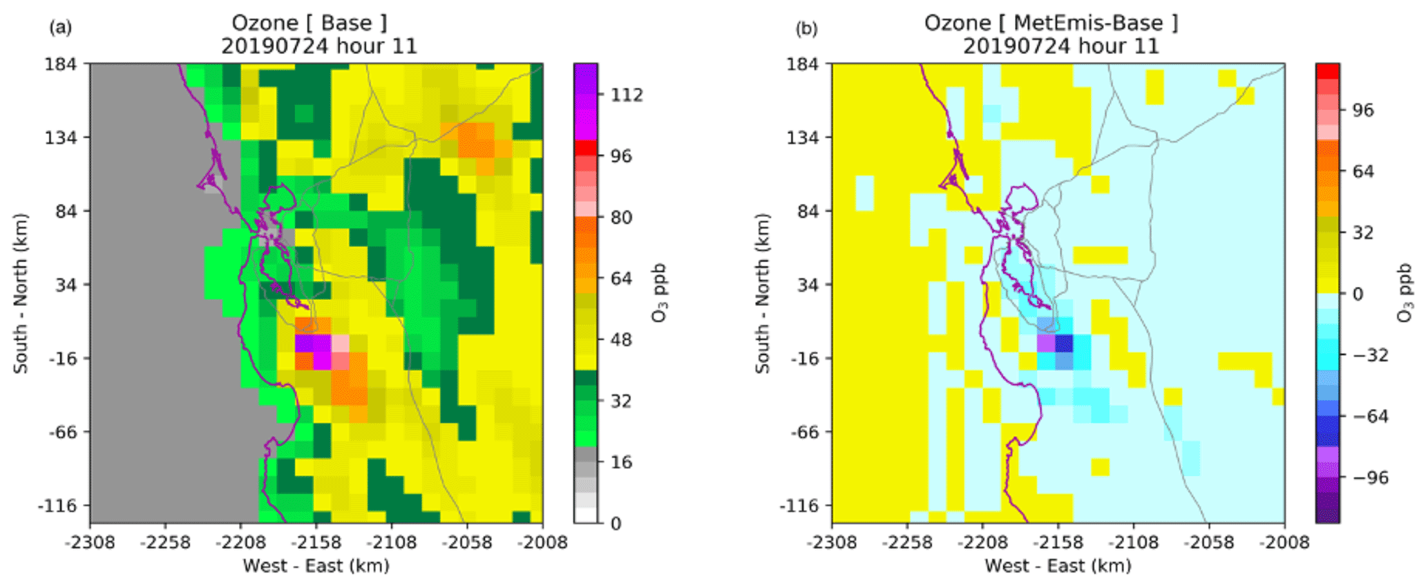
Figure 10Base hourly ozone concentration (ppb) (a) and the hourly ozone difference (MetEmis − Base) (b) at 11:00 LST on 24 July 2019.
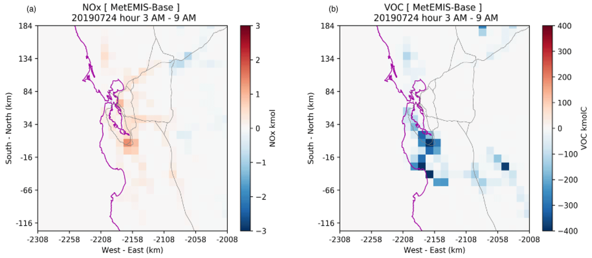
Figure 11Spatial differences in the NOx (a) and VOC (b) emissions from 03:00 to 09:00 LST on 24 July 2019 over San Jose, CA.
The PM2.5 simulation has similar patterns in January and July, with more particles concentrating in the east. The southwestern areas show less particulate pollution, as our emissions do not include natural sources such as dust storms and wildfires. The results from MetEmis present a slightly higher PM2.5 amount in the east because of the increased primary PM2.5 emissions. In addition, a decreased PM2.5 concentration is noted in California. This may be attributed to the fewer generated secondary aerosols, as the VOC emission is significantly reduced after adjustment.
Thus, this study further examines the influence of meteorology-induced mobile emission changes on modeling performance, which is particularly important for air quality forecasting in NAQFC. The 10 cities with the most changes in emissions are selected for comparison, as shown in Fig. 6. In general, noticeable improvement is found in the NO2 simulation with increasing R2 in all 10 cities, except for Detroit. San Jose and Atlanta exhibit the largest improvement in the NO2 simulation. Apparently, MetEmis successfully captured the daily variations in the mobile emissions, resulting in an improved temporal correlation. Meanwhile, the RMSEs were reduced in most of the cities (8 out of 10), suggesting the simulated biases can also be eliminated with MetEmis. Compared to NO2, the changes in O3 and PM2.5 are smaller due to the complex reactions. However, improvement is also found in summer with increased R2 and reduced RMSE in more than 70 % of cities, though less improvement is suggested in winter. We analyzed a few episodes with the largest changes for O3 and PM2.5 to demonstrate such an improvement.
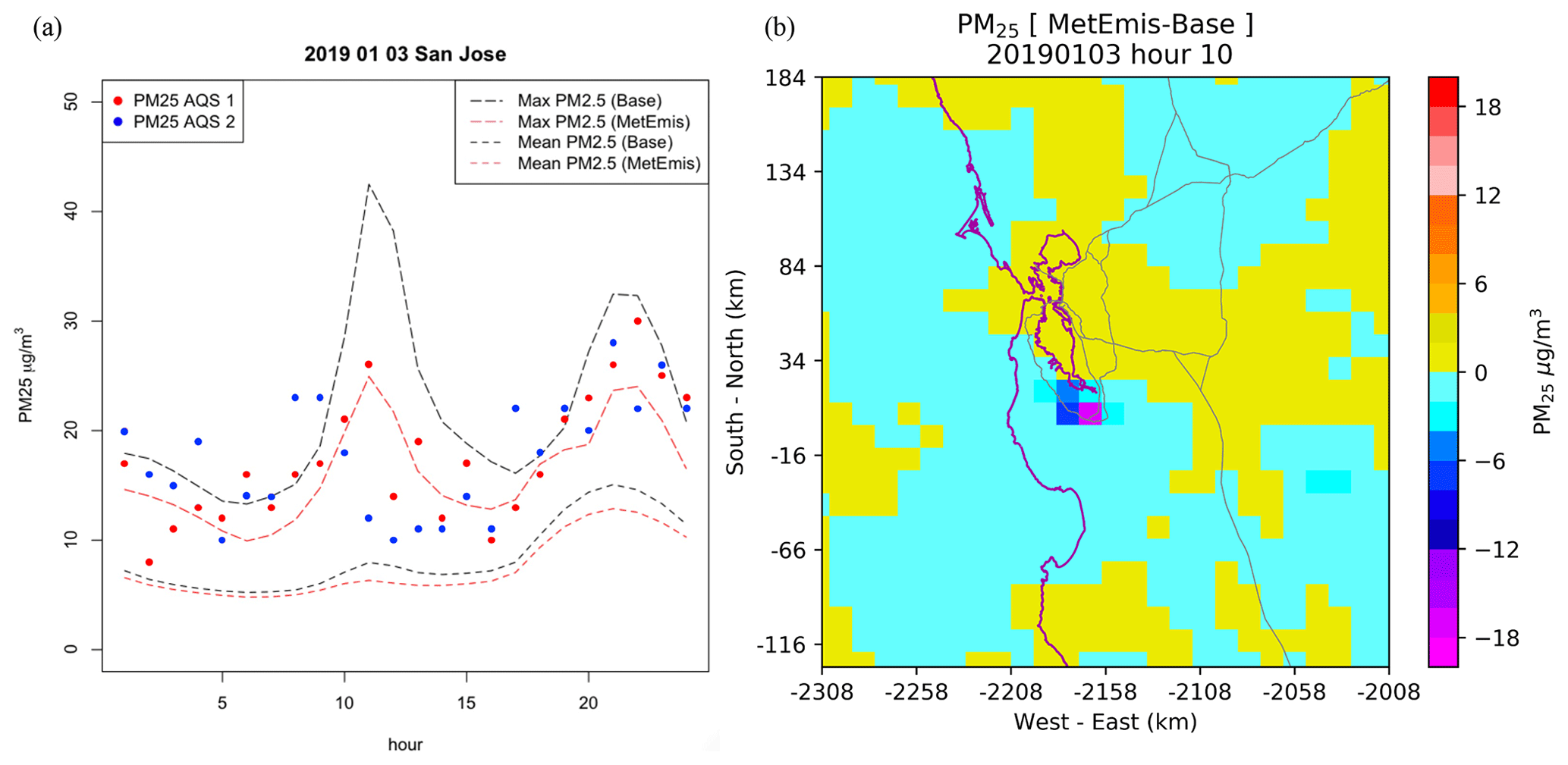
Figure 12(a) Diurnal variation in the PM2.5 (maximum and mean) concentrations over the targeted San Jose region, and (b) the spatial difference in the PM2.5 at 10:00 LST on 3 January 2019.
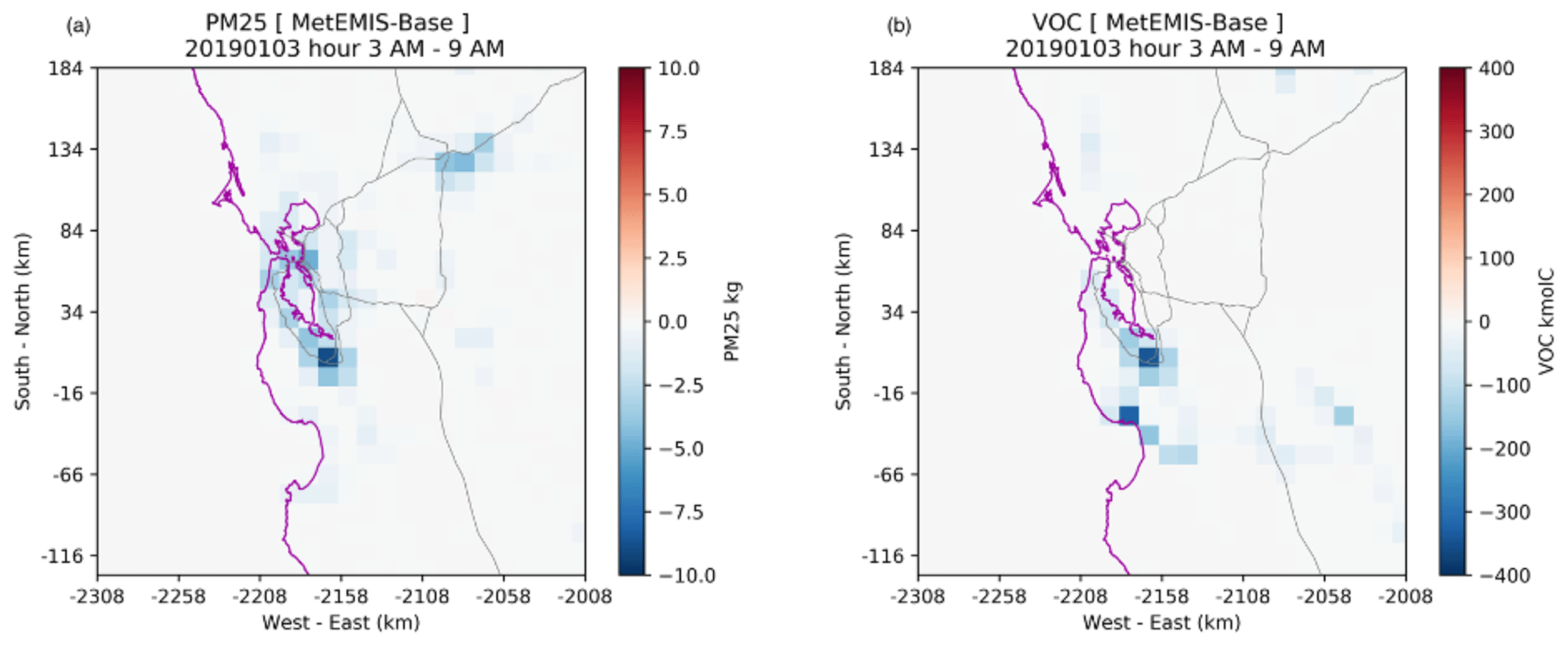
Figure 13Spatial difference in the PM2.5 (a) and VOC (b) emissions over the San Jose region from 03:00 to 09:00 LST on 3 January 2019.
3.2.3 Ozone episodic cases evaluation
Based on the July 2019 CMAQ simulation between the Base and MetEmis cases, we identified the locations where the largest changes in surface ozone occurred. Especially for July 2019, we witnessed a significant decrease in ozone over San Jose, CA, at 13:00 LST on 24 July 2019, while the greatest increase in ozone occurred over Chicago, IL, at 11:00 LST on 5 July 2019 (Table 4). Thus, we investigated these two episodes to understand the main drivers of these behaviors.
Largest ozone increase episode
Figure 7 shows the spatial ozone concentrations and the differences over the Chicago region between the Base and MetEmis scenarios at 11:00 LST on 5 July 2019. While the highest ozone amount occurred around the south of Lake Michigan in both scenarios (Fig. 7a), the largest ozone increase (∼ 7 ppb) is shown in the middle of Lake Michigan, where, unfortunately, there is no Air Quality System (AQS) monitoring location (Fig. 7b). To understand the cause of these ozone changes, we examined the differences in the NOx and VOC emissions between the Base and MetEmis scenarios. The increase in the VOC emissions from the MetEmis scenario in the early morning (03:00–09:00 LST) over the VOC-limited Chicago, IL, region seems to be the main driver of a significant increase in ozone (Fig. 8). Detailed information on the VOC and NOx concentration changes on 5 July 2019 is listed in Table 5. In the early morning, there was a decrease in the NOx concentration and an increase in VOC concentrations over the Chicago area. Due to no monitoring location being available over the lake, we could not properly perform the modeling evaluation statistics during the largest ozone increase.
Largest ozone decrease episode
There was a more than an 80 ppb ozone decrease over San Jose, CA, at 11:00 LST on 24 July 2019. To understand the cause of this significant decrease, we performed the analysis of precursor emission changes during the episode period. The colored green AQS locations are selected for the ozone concentration analysis, while the red ones are for the PM2.5 monitoring locations (Fig. 9a). Figure 9b shows the modeled hourly ozone concentrations (maximum, minimum, and mean) and AQS observations over the targeted (blue box) region from Fig. 9a. Figures 9b and 10 indicate that the maximum ozone values from the Base scenario clearly show an overestimated ozone over the San Jose, CA, downwind region, while the MetEmis case shows a significant improvement in the maximum ozone concentration during the daytime. The main driver of this significant ozone change over the targeted San Jose area is due to the substantial reduction in the VOC emissions in MetEmis from Base (Fig. 11a). The statistics of the NOx and VOC concentrations from CMAQ in Table 6 show consistent findings.
3.2.4 PM2.5 episodic case evaluation
Along with the significant ozone decrease in July 2019, there was a significant PM2.5 decrease from the CMAQ-MetEmis simulation from 42.5 (Base) to 25 µg m−3 at 10:00 LST on 3 January 2019. Approximately 17.5 µg m−3 (>41 %) PM2.5 decrease was witnessed in CMAQ-MetEmis simulations (Fig. 11). The CMAQ-MetEmis simulation shows a significant improvement in the modeled PM2.5 concentration when compared to the ones from the AQS monitoring locations from Fig. 8a (Fig. 12a). The main cause of this PM2.5 decrease in CMAQ-MetEmis is mainly a significant decrease in primary PM2.5 and VOC emissions (Fig. 13). Primary hourly PM2.5 emissions from the MetEmis scenario were significantly lowered, when compared to the ones from the Base scenario, by approximately a maximum of 20 kg h−1 from 03:00 to 09:00 LST on 3 January 2019.
To address the limitation of a traditional estimation for on-road vehicle emissions, this study developed a novel method (i.e., MetEmis) by dynamically coupling the meteorology-induced on-road emissions with simulated meteorological data in the air quality modeling system, which significantly improves both the computational efficiency and accuracy. The computational time for processing 1 d on-road emission data is substantially reduced from 1.9 h offline to less than 1 min inline, enabling the on-road emission estimates to be simultaneously coupled with the meteorology forecasting. Overall, MetEmis corrected the low biases of NOx and primary PM2.5 emissions domain-wide and high biases of VOC emissions in California. MetEmis also successfully captured the temporal variation in the on-road vehicle emissions, resulting in improved simulated NO2, O3, and PM2.5 concentrations, with more agreement with observations compared to the ones using static temporal profiles. Particularly, the simulated NO2 concentration exhibits noticeable improvement with increased R2 and decreased RMSEs in most cities. The simulated O3 and PM2.5 concentrations were also improved, particularly in summer.
The newly developed CMAQ-MetEmis model demonstrates the importance of dynamic coupling emissions and meteorological forecasting. While this study only focused on the on-road emissions, other meteorology-induced sectors such as residential combustion and agricultural livestock are planned to be included in the MetEmis development as well to represent the meteorological influence on all meteorologically induced anthropogenic emissions. Meanwhile, this study mainly focuses on replicating the same dynamic emissions from the offline SMOKE-MOVES on-road mobile emissions for the CMAQ model as the inline option. The native uncertainties from the MOVES model still exist and may lead to the uncertainties in the temporal profile estimated in MetEmis, which need be further improved in future studies.
The source codes of the SMOKE and the CMAQ models for MetEmis coupler can be downloaded from https://doi.org/10.5281/zenodo.7150000 (Baek, 2022).
All the datasets, spreadsheets, and Python scripts used in this paper for the data analysis are available at https://doi.org/10.5281/zenodo.7150000 (Baek, 2022).
BHB is the lead researcher in this study, and BHB and CC developed the source codes of CMAQ-MetEmis. SM, CTW, YL, JX, and DT prepared the modeling inputs and analyzed the modeling results. JHW and SK participated in the design of the weather-aware emission modeling system.
The contact author has declared that none of the authors has any competing interests.
Publisher’s note: Copernicus Publications remains neutral with regard to jurisdictional claims in published maps and institutional affiliations.
This research has been funded by the National Oceanic and Atmospheric Administration (NOAA)'s Office of Weather and Air Quality (OWAQ) to improve the National Air Quality Forecasting Capability (NAQFC; grant no. NOAA-OAR-OWAQ-2019-2005820) and the National Strategic Project – Fine Particle of the National Research Foundation (NRF) of the Republic of Korea, which is funded by the Ministry of Science and Information and Communications Technology (MSIT), the Ministry of Environment (ME), the Ministry of Health and Welfare (MOHW; grant no. NRF-2020M3G1A1114621), and by the Republic of Korea Environmental Industry & Technology Institute (KEITI) through the Public Technology Program based on Environmental Policy Program, funded by the Republic of Korea Ministry of Environment (MOE; grant no. 2022003560007).
This research has been supported by the National Oceanic and Atmospheric Administration (grant no. NOAA-OAR-OWAQ-2019-2005820), the National Research Foundation of the Republic of Korea (grant no. 2020M3G1A1114621), and the Republic of Korea Environmental Industry and Technology Institute (grant no. 2022003560007).
This paper was edited by Jason Williams and reviewed by two anonymous referees.
Andrade, M. d. F., Kumar, P., de Freitas, E. D., Ynoue, R. Y., Martins, J., Martins, L. D., Nogueira, T., Perez-Martinez, P., de Miranda, R. M., Albuquerque, T., Gonçalves, F. L. T., Oyama, B., and Zhang, Y.: Air quality in the megacity of São Paulo: Evolution over the last 30 years and future perspectives, Atmos. Environ., 159, 66–82, https://doi.org/10.1016/j.atmosenv.2017.03.051, 2017.
Baek, B. H.: The Integration approach of MOVES and SMOKE models, the 19th Emissions Inventory Conference, San Antonio, TX, https://gaftp.epa.gov/air/nei/ei_conference/EI20/session2/baek.pdf (last access: 28 July 2023), 2010.
Baek, B.: CMAQ-MetEmis: Development of Dynamic Meteorology-Induced Emissions Coupler (MetEmis) for Onroad Mobile Sources in the Community Multiscale Air Quality (CMAQ) (version 1.0), Zenodo [code and data set], https://doi.org/10.5281/zenodo.7150000, 2022.
Baek, B. H. and Seppanen, C.: CEMPD/SMOKE: SMOKE v4.8.1 Public Release (January 29, 2021), Zenodo [data set], https://doi.org/10.5281/zenodo.4480334, 2021.
Baek, B. H., Seppanen, C., Houyoux, M., Eyth, A., and Mason, R.: Installation Guide for the SMOKE-MOVES Integration Tool, https://www.cmascenter.org/smoke/documentation/0*moves_tool/SMOKE_MOVES_Tool_Installation_Guide.pdf (last access: 28 July 2023), 2010.
Byun, D. and Schere, K. L.: Review of the Governing Equations, Computational Algorithms, and Other Components of the Models-3 Community Multiscale Air Quality (CMAQ) Modeling System, Appl. Mech. Rev., 59, 51–77, https://doi.org/10.1115/1.2128636, 2006.
Chen, D., Liang, D., Li, L., Guo, X., Lang, J., and Zhou, Y.: The temporal and spatial changes of ship-contributed PM2.5 due to the inter-annual meteorological variation in Yangtze river delta, China, Atmosphere, 12, 722, https://doi.org/10.3390/atmos12060722, 2021.
Chen, W. H., Guenther, A. B., Wang, X. M., Chen, Y. H., Gu, D. S., Chang, M., Zhou, S. Z., Wu, L. L., and Zhang, Y. Q.: Regional to Global Biogenic Isoprene Emission Responses to Changes in Vegetation From 2000 to 2015, J. Geophys. Res.-Atmos., 123, 3757–3771, https://doi.org/10.1002/2017jd027934, 2018.
Choi, D., Beardsley, M., Brzezinski, D., Koupal, J., and Warila, J.: MOVES sensitivity analysis: the impacts of temperature and humidity on emissions, in: US EPA–Proceedings from the 19th Annual International Emission Inventory Conference, Ann Arbor, MI, 27–30 September 2010, https://www3.epa.gov/ttnchie1/conference/ei19/ (last access: 28 July 2023), 2010.
Dennis, R., Fox, T., Fuentes, M., Gilliland, A., Hanna, S., Hogrefe, C., Irwin, J., Rao, S. T., Scheffe, R., Schere, K., Steyn, D., and Venkatram, A.: A Framework for Evaluating Regional-Scale Numerical Photochemical Modeling Systems, Environ. Fluid Mech., 10, 471–489, https://doi.org/10.1007/s10652-009-9163-2, 2010.
Esri, HERE, TomTom, Intermap, increment P Corp., GEBCO, USGS, FAO, NPS, NRCAN, GeoBase, IGN, Kadaster NL, Ordnance Survey, Esri Japan, METI, Esri China (Hong Kong), swisstopo, MapmyIndia, and the GIS User Community: World Topographic Map, https://services.arcgisonline.com/ArcGIS/rest/services/World_Topo_Map/MapServer, (last access: 29 July 2023), 2013.
Fiore, A. M., Naik, V., Spracklen, D. V., Steiner, A., Unger, N., Prather, M., Bergmann, D., Cameron-Smith, P. J., Cionni, I., Collins, W. J., Dalsøren, S., Eyring, V., Folberth, G. A., Ginoux, P., Horowitz, L. W., Josse, B., Lamarque, J. F., MacKenzie, I. A., Nagashima, T., O'Connor, F. M., Righi, M., Rumbold, S. T., Shindell, D. T., Skeie, R. B., Sudo, K., Szopa, S., Takemura, T., and Zeng, G.: Global air quality and climate, Chem. Soc. Rev., 41, 6663–6683, https://doi.org/10.1039/c2cs35095e, 2012.
Foltescu, V. L., Pryor, S. C., and Bennet, C.: Sea salt generation, dispersion and removal on the regional scale, Atmos. Environ., 39, 2123–2133, https://doi.org/10.1016/j.atmosenv.2004.12.030, 2005.
Grell, G. and Baklanov, A.: Integrated modeling for forecasting weather and air quality: A call for fully coupled approaches, Atmos. Environ., 45, 6845–6851, https://doi.org/10.1016/j.atmosenv.2011.01.017, 2011.
Grell, G., Freitas, S. R., Stuefer, M., and Fast, J.: Inclusion of biomass burning in WRF-Chem: impact of wildfires on weather forecasts, Atmos. Chem. Phys., 11, 5289–5303, https://doi.org/10.5194/acp-11-5289-2011, 2011.
Hogrefe, C., Rao, S. T., Kasibhatla, P., Kallos, G., Tremback, C. J., Hao, W., Olerud, D., Xiu, A., McHenry, J., and Alapaty, K.: Evaluating the performance of regional-scale photochemical modeling systems: Part I – meteorological predictions, Atmos. Environ., 35, 4159–4174, https://doi.org/10.1016/S1352-2310(01)00182-0, 2001.
Iodice, P. and Senatore, A.: Cold Start Emissions of a Motorcycle Using Ethanol-gasoline Blended Fuels, Energy Procedia, 45, 809–818, https://doi.org/10.1016/j.egypro.2014.01.086, 2014.
Jacob, D. J. and Winner, D. A.: Effect of climate change on air quality, Atmos. Environ., 43, 51–63, https://doi.org/10.1016/j.atmosenv.2008.09.051, 2009.
Knippertz, P. and Todd, M. C.: Mineral dust aerosols over the Sahara: Meteorological controls on emission and transport and implications for modeling, Rev. Geophys., 50, 2011RG000362, https://doi.org/10.1029/2011rg000362, 2012.
Kumar, P., Patton, A. P., Durant, J. L., and Frey, H. C.: A review of factors impacting exposure to PM2.5, ultrafine particles and black carbon in Asian transport microenvironments, Atmos. Environ., 187, 301–316, https://doi.org/10.1016/j.atmosenv.2018.05.046, 2018.
Lathière, J., Hauglustaine, D. A., De Noblet-Ducoudré, N., Krinner, G., and Folberth, G. A.: Past and future changes in biogenic volatile organic compound emissions simulated with a global dynamic vegetation model, Geophys. Res. Lett., 32, L20818, https://doi.org/10.1029/2005GL024164, 2005.
Lee, P., McQueen, J., Stajner, I., Huang, J., Pan, L., Tong, D., Kim, H., Tang, Y., Kondragunta, S., Ruminski, M., Lu, S., Rogers, E., Saylor, R., Shafran, P., Huang, H.-C., Gorline, J., Upadhayay, S., and Artz, R.: NAQFC Developmental Forecast Guidance for Fine Particulate Matter (PM2.5), Weather Forecast., 32, 343–360, https://doi.org/10.1175/waf-d-15-0163.1, 2017.
Li, Q., Qiao, F., and Yu, L.: Vehicle Emission Implications of Drivers Smart Advisory System for Traffic Operations in Work Zones, J. Air Waste Manage., 11, 446–455, https://doi.org/10.1080/10962247.2016.1140095, 2016.
Lindhjem, C., Chan, L., Pollack, A., Corporation, E. I., Way, R., and Kite, C.: Applying Humidity and Temperature Corrections to On and Off-Road Mobile Source Emissions, in: 13th International Emission Inventory Conference, Clearwater, FL, 8–10 June 2004, https://www3.epa.gov/ttnchie1/conference/ei13/mobile/lindhjem.pdf (last access: 18 July 2023), 2004.
Liu, H., Guensler, R., Lu, H., Xu, Y., Xu, X., and Rodgers, M.: MOVES-Matrix for High-Performance On-Road Energy and Running Emission Rate Modeling Applications, J. Air Waste Manage., 69, 1415–1428, https://doi.org/10.1080/10962247.2019.1640806, 2019.
Luecken, D. J., Yarwood, G., and Hutzell, W. T.: Multipollutant modeling of ozone, reactive nitrogen and HAPs across the continental US with CMAQ-CB6, Atmos. Environ., 201, 62–72, https://doi.org/10.1016/j.atmosenv.2018.11.060, 2019.
Lv, Z., Liu, H., Ying, Q., Fu, M., Meng, Z., Wang, Y., Wei, W., Gong, H., and He, K.: Impacts of shipping emissions on PM2.5 pollution in China, Atmos. Chem. Phys., 18, 15811–15824, https://doi.org/10.5194/acp-18-15811-2018, 2018.
McDonald, B. C., McKeen, S. A., Cui, Y. Y., Ahmadov, R., Kim, S. W., Frost, G. J., Pollack, I. B., Peischl, J., Ryerson, T. B., Holloway, J. S., Graus, M., Warneke, C., Gilman, J. B., de Gouw, J. A., Kaiser, J., Keutsch, F. N., Hanisco, T. F., Wolfe, G. M., and Trainer, M.: Modeling Ozone in the Eastern U.S. using a Fuel-Based Mobile Source Emissions Inventory, Environ. Sci. Technol., 52, 7360–7370, https://doi.org/10.1021/acs.est.8b00778, 2018.
Mellios., G., Ntziachristos, L., Samaras, Z., White, L., Martini, G., and Rose, K.: EMEP/EEA air pollutant emission inventory guidebook 2019, Gasoline evaporation, European Environment Agency, https://www.eea.europa.eu/publications/emep-eea-guidebook-2019 (last access: 28 July 2023), 2019.
Pavlovic, R., Chen, J., Anderson, K., Moran, M. D., Beaulieu, P. A., Davignon, D., and Cousineau, S.: The FireWork air quality forecast system with near-real-time biomass burning emissions: Recent developments and evaluation of performance for the 2015 North American wildfire season, J. Air Waste Manage., 66, 819–841, https://doi.org/10.1080/10962247.2016.1158214, 2016.
Perugu, H.: Emission modelling of light-duty vehicles in India using the revamped VSP-based MOVES model: The case study of Hyderabad, Transport. Res. D-Tr. E., 68, 150–163, https://doi.org/10.1016/j.trd.2018.01.031, 2019.
Pierce, J. R. and Adams, P. J.: Global evaluation of CCN formation by direct emission of sea salt and growth of ultrafine sea salt, J. Geophys. Res.-Atmos., 111, D06203, https://doi.org/10.1029/2005JD006186, 2006.
Pouliot, G. A.: Emission processing for ETA/CMAQ, an air quality forecasting model, 7th Conference on Atmospheric Chemistry American Meteorological Society, San Diego, CA, 9–13 January 2005, https://cfpub.epa.gov/si/si_public_record_report.cfm?dirEntryId=116409&Lab=NERL (last access: 28 July 2023), 2005.
Rao, S. T., Galmarini, S., and Puckett, K.: Air Quality Model Evaluation International Initiative (AQMEII): Advancing the State of the Science in Regional Photochemical Modeling and Its Applications, B. Am. Meteorol. Soc., 92, 23–30, https://doi.org/10.1175/2010BAMS3069.1, 2011.
Skamarock, C., Klemp, B., Dudhia, J., Gill, O., Liu, Z., Berner, J., Wang, W., Powers, G., Duda, G., Barker, D., and Yu Huang, X.: A Description of the Advanced Research WRF Model Version 4.3, NCAR/TN-556+STR, NCAR, https://doi.org/10.5065/1dfh-6p97, 2021.
Tang, Y., Pagowski, M., Chai, T., Pan, L., Lee, P., Baker, B., Kumar, R., Delle Monache, L., Tong, D., and Kim, H.-C.: A case study of aerosol data assimilation with the Community Multi-scale Air Quality Model over the contiguous United States using 3D-Var and optimal interpolation methods, Geosci. Model Dev., 10, 4743–4758, https://doi.org/10.5194/gmd-10-4743-2017, 2017.
Tong, D. and Mauzerall, D. L.: Spatial variability of summertime tropospheric ozone over the continental United States: Implications of an evaluation of the CMAQ model, Atmos. Environ., 40, 3041–3056, 2006.
Tong, D., Lee, P., and Saylor, R.: New Direction: The need to develop process-based emission forecasting models, Atmos. Environ., 47, 560–561, https://doi.org/10.1016/j.atmosenv.2011.10.070, 2012.
Tong, D., Lamsal, L., Pan, L., Ding, C., Kim, H., Lee, P., Chai, T., Pickering, K. E., and Stajner, I.: Long-term NOx trends over large cities in the United States during the great recession: Comparison of satellite retrievals, ground observations, and emission inventories, Atmos. Environ., 107, 70–84, https://doi.org/10.1016/j.atmosenv.2015.01.035, 2015.
U.S. EPA: Derivation of humidity and NOx humidity correction factors, https://www.epa.gov/sites/default/files/2015-09/documents/noxcorr.pdf (last access: 18 July 2023), 1997.
U.S. EPA: Emission Adjustments for Temperature, Humidity, Air Conditioning, and Inspection and Maintenance for on-Road Vehicles in MOVES2014, https://ntrl.ntis.gov/NTRL/dashboard/searchResults/titleDetail/PB2017101384.xhtml (last assess: 28 July 2023), 2015.
U.S. EPA: Overview of EPA’s MOtor Vehicle Emission Simulator (MOVES3), Office of Transportation and Air Quality, EPA-420-R-21-004, US Environmental Protection Agency, https://nepis.epa.gov/Exe/ZyPDF.cgi?Dockey=P1011KV2.pdf (last access: 28 July 2023), 2021a.
U.S. EPA: O2017 National Emissions Inventory: January 2021 Updated Release, Technical Support Document, Office of Air Quality Planning and Standards, EPA-454/R-21-001, US Environmental Protection Agency, https://www.epa.gov/sites/default/files/2021-02/documents/nei2017_tsd_full_jan2021.pdf (last access: 28 July 2023), 2021b.
Wong, K. W., Tsai, C., Lefer, B., Haman, C., Grossberg, N., Brune, W. H., Ren, X., Luke, W., and Stutz, J.: Daytime HONO vertical gradients during SHARP 2009 in Houston, TX, Atmos. Chem. Phys., 12, 635–652, https://doi.org/10.5194/acp-12-635-2012, 2012.
Xu, X., Liu, H., Anderson, J. M., Xu, Y., Hunter, M. P., Rodgers, M. O., and Guensler, R. L.: Estimating Project-Level Vehicle Emissions with Vissim and MOVES-Matrix, Transp. Res. Record, 2570, 107–117, https://doi.org/10.3141/2570-12, 2016.