the Creative Commons Attribution 4.0 License.
the Creative Commons Attribution 4.0 License.
 | 11 Aug 2023
ENSO statistics, teleconnections, and atmosphere–ocean coupling in the Taiwan Earth System Model version 1
Yi-Chi Wang
Yu-Luen Chen
Shih-Yu Lee
Huang-Hsiung Hsu
Hsin-Chien Liang
This study provides an overview of the fundamental statistics and features of the El Niño–Southern Oscillation (ENSO) in the historical simulations of the Taiwan Earth System Model version 1 (TaiESM1). Compared with observations, TaiESM1 can reproduce the fundamental features of observed ENSO signals, including seasonal phasing, thermocline coupling with winds, and atmospheric teleconnection during El Niño events. However, its ENSO response is approximately 2 times stronger than observed in the spectrum, resulting in powerful teleconnection signals. The composite of El Niño events shows a strong westerly anomaly extending fast to the eastern Pacific in the initial stage in March, April, and May, initiating a warm sea surface temperature anomaly (SSTA) there. This warm SSTA is maintained through September, October, and November (SON) and gradually diminishes after peaking in December. Analysis of wind stress–SST and heat flux–SST coupling indicates that biased positive SST–shortwave feedback significantly contributes to the strong warm anomaly over the eastern Pacific, especially in SON. Our analysis demonstrates TaiESM1's capability to simulate ENSO – a significant tropical climate variation on interannual scales with strong global impacts – and provides insights into mechanisms in TaiESM1 related to ENSO biases, laying the foundation for future model development to reduce uncertainties in TaiESM1 and climate models in general.
- Article
(8596 KB) - Full-text XML
-
Supplement
(1329 KB) - BibTeX
- EndNote


The El Niño–Southern Oscillation (ENSO) is the primary mode of interannual and decadal climate variability in the tropics (Glantz, 2001; McPhaden et al., 2006). It also affects climate variations in subtropical and midlatitude regions across both hemispheres through teleconnection of Rossby waves (Diaz et al., 2001; Yeh et al., 2018). Therefore, its prediction is an essential part of global climate prediction on these scales (Latif et al., 1998). Additionally, ENSO is a crucial metric for climate model evaluation, especially for atmosphere–ocean coupling and associated physical feedbacks (Planton et al., 2021). Many studies have reported that Coupled Model Intercomparison Project (CMIP) models have successfully represented the basic features of observed ENSO, such as a recognizable ENSO life cycle and sea surface temperature (SST) pattern over the tropical central and eastern Pacific (Guilyardi et al., 2009, 2020; Lloyd et al., 2009, 2011; Bellenger et al., 2014). However, many model biases are also found in CMIP6 models (Beobide-Arsuaga et al., 2021; Capotondi et al., 2020a; Chen and Jin, 2021), resulting in 30 %–50 % uncertainties in future ENSO projection (Beobide-Arsuaga et al., 2021).
The paradigm based on theory and observations depicts ENSO as a closely coupled oscillation system between the ocean and the atmosphere (Jin, 1997; Latif et al., 1998; McPhaden et al., 1998, 2006; Neelin et al., 1998; Philander, 1989; Wang, 2018; Wang and Picaut, 2013). An El Niño event begins from a westerly wind initiated over the western equatorial Pacific, typically in the spring of the first year (i.e., March, April, and May in year 0; MAM0). The westerly wind drives more warm water towards the east and gradually warms the central Pacific. Around summer, eastward-propagating oceanic Kelvin waves are triggered over the central Pacific, reducing the upwelling at the tropical eastern Pacific, deepening the thermocline, and warming the sea surface temperature (SST). Consequently, the zonal SST gradient and the easterly wind in the tropical Pacific are reduced. Such a retreat of the easterly wind further reduces the SST gradient, causing the so-called Bjerknes feedback between the easterly wind and the SST gradient (Bjerknes, 1969; Cane, 2005). Through this feedback, the warm SST increases and reaches a maximum around the following winter (i.e., December of year 0 and January and February of year 1; DJF+1). Furthermore, following the warm SST anomaly (SSTA), the center of deep convection activity shifts toward the central Pacific, increasing latent heat flux and reducing shortwave heat flux into the ocean surface through deep cloud cover. Such seasonal phase locking of an El Niño event is a crucial characteristic of the observed ENSO.
In contrast to the coupling nature of the atmosphere and ocean found in ENSO observations, the atmospheric feedbacks are found to dominate the modeled ENSO frequency and amplitude in CMIP models (Guilyardi et al., 2009; Lloyd et al., 2009, 2011; Bellenger et al., 2014; Beobide-Arsuaga et al., 2021). It has been noticed that the CMIP models tend to simulate a weaker Bjerknes feedback, namely, a weaker SST warming and westerly wind coupling. Furthermore, the heat flux–SST feedbacks are overemphasized in simulated ENSO dynamics, especially for the shortwave heat flux–SST feedback. Such overemphasized heat flux–SST feedback compensates for the weaker warming from the Bjerknes feedback, producing a seemingly realistic ENSO warming in CMIP models (Bayr et al., 2019). The biased Bjerknes and heat flux feedbacks were later found to be related to the biases of the seasonal variations of Walker circulation (Bayr et al., 2019, 2018). Such complexity resulting from intertwined atmospheric–ocean feedbacks makes it challenging for model developers to improve ENSO simulations without fully understanding how these mechanisms are represented in the coupled models.
Taiwan Earth System Model version 1 (TaiESM1; Lee et al., 2020) is the Earth system model developed at the Research Center for Environmental Changes (RCEC), Academia Sinica. It participates in the CMIP6 intercomparison activity and has been used to study major climate variabilities and regional climate features (Chen and Jin, 2021; Park et al., 2020). While its overall performance of climate mean states and major variations has been evaluated and documented in Wang et al. (2021), in this study, we conducted a more comprehensive investigation of ENSO's fundamental features and statistics in historical TaiESM1 simulations. We noticed that the ENSO amplitude increased significantly compared with the observations, with intense and prolonged warm SST from May to December. Especially over the eastern Pacific, the early onset of warming and sustained warming in September, October, and November (SON0) before peaks in December are the two primary prominent biases. We further analyzed the physical processes associated with ENSO's strong warming biases and found it is due to the biased positive feedback between SST and shortwave surface fluxes over the eastern equatorial Pacific. Such feedback is primarily attributed to the prevailing low clouds overlying the cold tongue region, with large cold biases in SON0. Our results provide the baseline for ENSO performance in TaiESM1 and suggest that the current ENSO biases in TaiESM1 are intertwined with biases of the mean state and seasonal variation of the tropical climate system. The remainder of this study includes the following. Section 2 describes the TaiESM1 and observational dataset used for model evaluation and the methodology for analyzing ENSO. Section 3 documents the basic characteristics of ENSO simulated in TaiESM1. More analysis focuses on seasonal variation of El Niño events in TaiESM1 and associated biases in Sect. 4. The study is concluded with a summary and discussion in Sect. 5.
Based on the Community Earth System Model version 1.2.2 (CESM1.2.2; Hurrell et al., 2013) developed by the National Center for Atmospheric Research and sponsored by the National Science Foundation and the Department of Energy in the United States, TaiESM1 includes several physical schemes developed in-house in RCEC. These designs include convective triggering (Y. C. Wang et al., 2015), radiation parameterization of three-dimensional topography (Lee et al., 2013), an aerosol scheme (Chen et al., 2013), and a cloud fraction scheme based on probability density function (Shiu et al., 2021). The ocean component is the same as CESM1 using the Parallel Ocean Program version 2 (POP2; Smith et al., 2010). An overall evaluation of climate variability in TaiESM1 shows that the simulated ENSO features stronger SST warming and atmospheric teleconnection compared with the base model CESM1 (Wang et al., 2021). In this study, we have conducted a more in-depth analysis of ENSO's fundamental features and statistics and identified the physical processes of ENSO biases within TaiESM1. The historical simulation of TaiESM1 from 1850 to 2014, driven by the forcing designed by CMIP6, is analyzed. The historical run is initiated from the pre-industrial control run of TaiESM1. It utilizes an atmospheric model with a horizontal resolution of 0.9∘ latitude × 1.25∘ longitude and 30 vertical layers. The community land model employed shares the same resolution as the atmospheric model. Additionally, the POP2 ocean model has a resolution of approximately 1.125∘ in longitude and 0.47∘ in latitude.
We evaluated the model's performance using the atmospheric variables from the Collaborative Reanalysis Technical Environment Multireanalysis Ensemble version 2 (MRE2; Potter et al., 2018). The MRE2 is a product of the ensemble average of seven reanalysis products, including CFSR (Saha et al., 2010), ERA-Interim (Dee et al., 2011), MERRA (Rienecker et al., 2011), MERRA-2 (Gelaro et al., 2017), JRA-25 (Onogi et al., 2007), JRA-55 (Kobayashi et al., 2015), and 20CRv2c (Compo et al., 2011). Studies have found that the ensemble average can reduce the errors of individual reanalysis for selected atmospheric variables (Potter et al., 2018). For those variables not provided in MRE2, such as cloud cover, we used the ECMWF reanalysis version 5 (ERA5), the most up-to-date reanalysis produced by ECMWF (Hersbach et al., 2020). While previous studies have identified differences in air–sea feedbacks among reanalysis datasets, the ensemble mean of multiple reanalysis datasets can be used as the best estimate by reducing random errors through averaging (Kumar and Hu, 2012). We also obtained precipitation data from the Global Precipitation Climatology Project (GPCP V2; Adler et al., 2003; Huffman et al., 2009), SST data from the Extended Reconstructed SST version 5 (ERSSTv5; Huang et al., 2017), and subsurface ocean data, such as sea surface height (SSH) and potential subsurface temperature, from the Simple Ocean Data Assimilation version 3.3.2 (SODA v3.3.2; Carton et al., 2018). The observational datasets used for this study span 1980 to 2018, except for ERSST, which covers the period from 1900 to 2018.
In this study, we employ regression and composite analyses as the primary tools to investigate ENSO features. We represent El Niño using indices over crucial regions, including Niño 3 (5∘ N–5∘ S, 150–90∘ W), Niño 3.4 (5∘ N–5∘ S, 170–120∘ W), and Niño 4 (5∘ N–5∘ S, 160∘ E–150∘ W), in the regression analysis. For the observational Niño 3.4 index, we use a base period between 1900 and 2014 from ERSSTv5, following the Niño index calculation of the Climate Prediction Center, NOAA (NOAA Climate Prediction Center, 2000). We also use model data from 1900 to 2014 as the base period for TaiESM1's historic run. To avoid impacts of model bias on longer timescales, such as interdecadal variation, we utilize the full length of available simulation data to obtain the most robust statistics of ENSO feature simulated by TaiESM1.
We choose the composite method instead of the regression map to better identify teleconnection signals associated with the El Niño events. In our preliminary analysis, the regressed maps of El Niño events show patterns similar to the composite events in the tropics, but with much weaker signals in the midlatitudes (not shown). Furthermore, as the ENSO events simulated in TaiESM1 show very symmetric alternations between El Niño and La Niña events, our composite based on El Niño events is followed by La Niña events. To build the El Niño composite, we choose strong events with the Niño 3.4 index larger than 1 standard deviation (i.e., 1.22 ∘C) over the simulation period. The ERSSTv5 dataset includes eight El Niño events in 1982, 1986, 1987, 1991, 1994, 1997, 2002, and 2009. In comparison, TaiESM1 simulated 21 events throughout the entire historical simulation. As the El Niño events simulated by TaiESM1 exhibit a very strong amplitude, most of the composite fields of these events passed the significance test at the 95 % confidence level (not shown). Therefore, we will not denote regions passing significant tests in the composite fields in the following analysis.
In our analysis of TaiESM1's ability to simulate ENSO diversity, we examined its capability to distinguish between eastern Pacific (EP) and central Pacific (CP) El Niño events using the Niño 3–Niño 4 approach (Kug et al., 2009). During the historical period of TaiESM1, we identified 23 CP events and 17 EP events. This higher frequency of CP events in TaiESM1 is consistent with previous findings in CMIP models (Capotondi et al., 2020b; Chen et al., 2017; McPhaden et al., 2011). It is worth noting that the total number of El Niño events exceeds 21 when using the El Niño 3.4 index, as some EP events transition into CP events during the mature phase. In contrast, during the observation period from 1980 to 2014, we found a total of four EP events and four CP events. In the subsequent sections, we will also discuss the composites of EP and CP events in further detail.
3.1 Niño 3.4 SST variability
Figure 1 shows the mean SST state (white contour) and monthly standard deviation (color shading) in ERSST and TaiESM1 over the tropical Pacific. The monthly standard deviation denotes the deviation of monthly SSTs from long-term monthly mean SST. TaiESM1 has a much more substantial equatorial Pacific SST variability, with an elongated region of high SST variation extending further into the warm pool region. Such a westward extension is collocated with the equatorial cold tongue, indicated by the 27 ∘C isotherm thick white contour laying over the tropical eastern Pacific in the climatological SST mean field. TaiESM1 simulated a westward extension of the cold tongue compared with ERSSTv5. TaiESM1 also overestimated SST variation over other tropical oceans, including the Indian Ocean and warm pool.
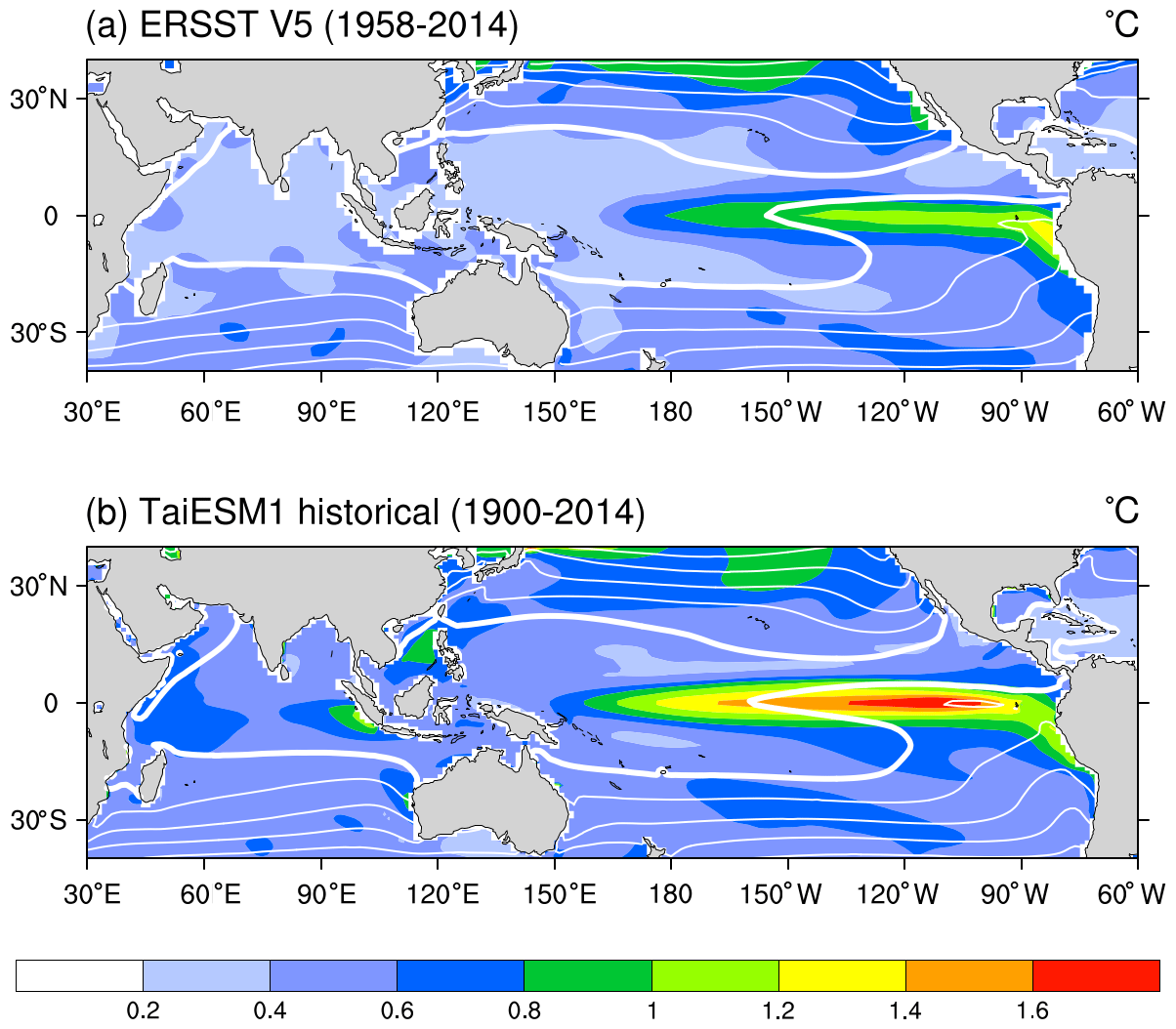
Figure 1Mean SST (white contours) and SST monthly standard deviation (color shading) for (a) detrended ERSSTv5 over 1958–2014 and (b) 1900–2014 of the TaiESM1 historical simulations. The contour interval is 3 ∘C, and the thick white contour indicates the 27 ∘C isotherm.
Figure 2 shows the Niño 3.4 SST index based on the ERSSTv5 and TaiESM1 historical simulations. TaiESM1 has more oscillatory ENSO signals with alternating cold and warm phases during 3–5 years compared with the observations. The Niño 3.4 index's standard deviation of ERSSTv5 is 0.84 ∘C, whereas that of TaiESM1 is 1.22 ∘C. The simulated ENSO amplitude decreased after 1980 when the global temperature increased (Fig. 2a, b). When comparing SST and surface wind fields between two 30-year periods, specifically 1950–1980 and 1984–2014, during which TaiESM1 exhibits distinct ENSO variability, Fig. S1 demonstrates a notable shift in the background state towards a La Niña-like state. This shift is characterized by an increased zonal temperature gradient over the tropical Pacific and strengthened trade winds during the period of 1984–2014 in comparison to the period of 1950–1980. Previous studies investigating the ENSO response to changes in the observed mean state have indicated that such an increase in zonal wind stress can lead to a weakening of feedback mechanisms associated with El Niño (Fedorov et al., 2020; Zhao and Fedorov, 2020). This aligns with the observed decrease in ENSO variability in TaiESM1 during the period of 1984–2014.
The power spectrum of Niño 3.4 confirms what is found in the time series of Niño 3.4, namely a much larger amplitude of ENSO in TaiESM1 (Fig. 2c). The amplitude of major peak between 3 and 4 years is around 250 ∘C2 per month, while that of observed peak is around 75 ∘C2 per month in ERSSTv5. Similarly, around the secondary peak with a period of 5 to 6 years in observations, TaiESM1 also shows two spectral peaks at 6 years and 8 years with stronger amplitude, respectively. Such model bias in representing ENSO-related spectral peaks has long been noticed in CMIP models and is still one of most challenging questions for climate models (Jha et al., 2014). Figure 2d shows the seasonal cycle of ENSO SST variance in ERSSTv5 and TaiESM1. Compared with the observations, the peak months simulated by TaiESM1 occurred in boreal winter, with a 1-month delay from the observed and a larger amplitude that was 1.5 times the observed value.
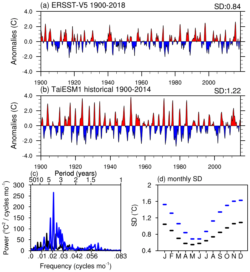
Figure 2Normalized time series of Niño 3.4 index in (a) ERSSTv5 (1900–2018) and (b) the TaiESM1 historical run (1900–2014). The standard deviation of each dataset is noted on the upper-right side of the panels. The corresponding spectrums are shown in (c), with a black line for ERSSTv5 and a blue line for TaiESM1. (d) The seasonal cycle of SST variance in ERSSTv5 (black) and TaiESM1 (blue).
3.2 Atmosphere–ocean coupling of ENSO
As a coupled oscillation system, the coupling of atmosphere and ocean plays an important role in ENSO dynamics. To see how such coupling is simulated in TaiESM1, Fig. 3 shows the regressed rainfall, wind stress, and SST to the Niño 3.4 index in the observations (Fig. 3a) and TaiESM1 (Fig. 3b). In Fig. 3a, the observation shows the west–east displacement of wind stress and warm SST over the tropical Pacific. The strong wind stress at 160∘ E is collocated with rainfall due to (mostly meridional) moisture convergence at the west and north edges of the warm SSTA, which was located in the central-eastern equatorial Pacific and was approximately 1∘ higher than the western equatorial Pacific. It is important to note that the major sea surface temperature anomaly (SSTA) did not occur in the eastern equatorial Pacific, where interannual variance was the highest. Instead, the SSTA occurred to the west of the region with the maximum variance. In TaiESM1 (as shown in Fig. 3b), the warm SST center is located at approximately 120∘ W, which is further east than in the observational data. Moreover, the magnitude of the SST anomaly is approximately 50 % greater in TaiESM1 than in the observations. Compared with ERSST, the warm SSTA in TaiESM1 is meridionally narrower and more zonally elongated to the western Pacific around 155∘ E, causing stronger zonal and meridional SST gradients. An increase in the meridional SST gradient induces stronger meridional wind and moisture convergence over the equatorial Pacific. Zonally, the stronger westerly wind extends wider from 155∘ E to 120∘ W near the eastern edge of the island of New Guinea. As a result, TaiESM1 produces strong wind stress and more deep convection (shown by rainfall; color shading in Fig. 3) to the north and west sides of the warm SSTA. Figure S2 shows the regressed magnitude of wind stress onto the Niño 3.4 index and marks longitude center with dashed lines. While TaiESM1 reproduces the longitudinal center of wind stress response at 140∘ E as in observations, the response magnitude of wind stress to SST increase is weaker in TaiESM1 than in the observations.
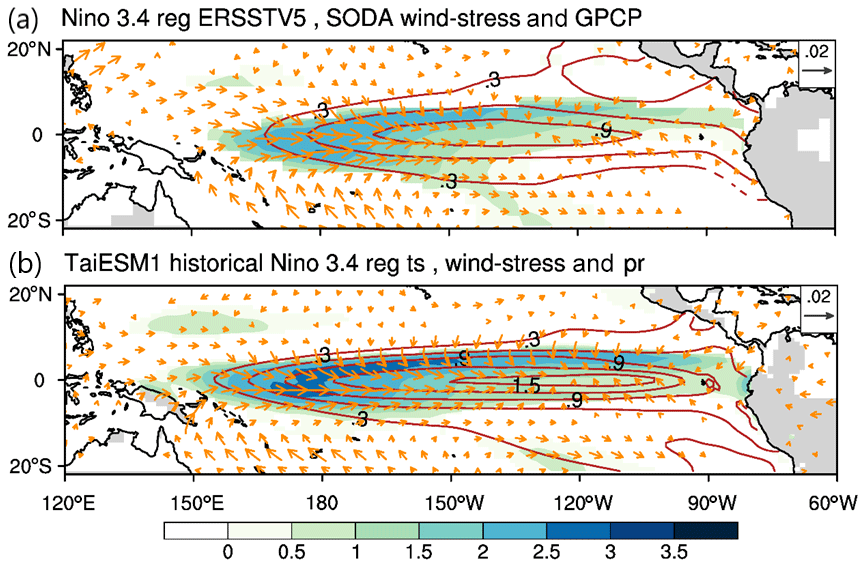
Figure 3Regression map of precipitation (mm d−1, color shading), wind stress (s−1, vectors), and sea surface temperature (SST; ∘C, contours) on the normalized Niño 3.4 index for (a) the Global Precipitation Climatology Project (GPCP), Simple Ocean Data Assimilation (SODA), Extended Reconstructed SST (ERSST), and (b) TaiESM1 historical simulation.
Figure 4 shows the regressed SSH to the wind stress averaged over the Niño 3 region (5∘ N–5∘ S, 150∘ E–90∘ E) to show the thermocline response to the strengthening of equatorial wind stress over the western Pacific. In the observation, a west–east dipole of thermocline response is found in Fig. 4a, showing thermocline deepening over the eastern Pacific (marked as black square in Fig.4) and shallowing over the western subtropical Pacific. Compared with the observations, TaiESM1 has captured this west–east dipole of SSH response to equatorial wind stress, but with a much stronger magnitude over the eastern equatorial Pacific (Fig. 4b). Such a strong response indicates that the SSH in TaiESM1 is more responsive than the observed to the wind stress and can easily lead to an El Niño state through the Bjerknes feedback by reducing the zonal SST gradient when the wind stress anomaly in the central equatorial Pacific initiates.
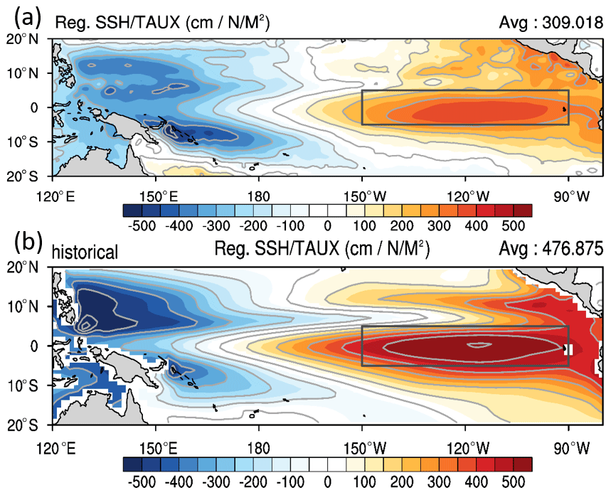
Figure 4Regression map of sea surface height (SSH, cm N−1 m2, color shading) upon the normalized wind stress averaged over the Niño-4 region of 5∘ S–5∘ N and 160∘ E–160∘ W (a) from Simple Ocean Data Assimilation (SODA) and (b) the historical run of TaiESM1. The black square represents the Niño 3 region.
In addition to the two components of atmosphere–ocean coupling related to the wind stress, we also examine the heat flux–SST coupling related to ENSO. Figure 5a and b show the shortwave radiation regressed to the Niño 3.4 index in MRE2 and TaiESM1. In the observations, the reduction in shortwave fluxes prevails in the tropics with an increased warm SSTA in the Niño 3.4 region because of emerging deep convection reflecting more shortwave radiation back (Fig. 5a). A zonal gradient of shortwave fluxes is shown from −160 W m−2 K−1 over the western Pacific (i.e., 170∘ E) to −80 W m−2 K−1 over the eastern Pacific (i.e., 120∘ W). Overall, TaiESM1 reproduced the negative feedback patterns in the deep tropics (3∘ S–3∘ N), but with a much stronger shortwave reduction of −200 W m−2 K−1 over the western Pacific in response to the warm SSTA in the Niño 3.4 region (Fig. 5b). Such a pattern is consistent with a stronger rainfall response of TaiESM1 in Fig. 3b, suggesting that the stronger deep convection response reflects more shortwave fluxes over the western Pacific. In contrast, we observed an increase in downwelling shortwave flux over the subsidence regions adjacent to the Intertropical Convergence Zone (ITCZ) at both 10∘ N and 10∘ S over the eastern Pacific. One notable feature in TaiESM1 is that the shortwave fluxes can increase up to 60 W m−2 K−1 over the tropical eastern Pacific (i.e., 120 to 100∘ W), in contrast to a decrease in observations (Fig. 5). Such a difference suggests that there is a biased cloud radiative response over the eastern Pacific when an El Niño event occurs, which may induce biased heat flux–SST coupling in TaiESM1. We will further examine and discuss this bias in Sect. 4.
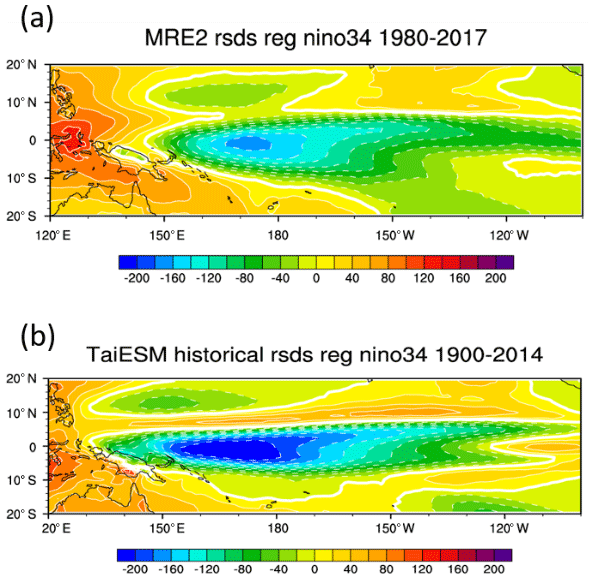
Figure 5Regression map of tropical surface downwelling shortwave radiation (RSDS; W m−2; color) upon the normalized Niño 3.4 index for (a) the MRE2 ensemble (1980–2017) and (b) TaiESM1 historical simulation (1900–2014).
3.3 Composite of El Niño structure and teleconnection
To evaluate the structure of El Niño events in TaiESM1, we compile strong El Niño events with a Niño 3.4 index larger than 1 standard deviation of the entire time series (i.e., larger than 1.22 ∘C). Under this definition, there are 21 Niño events in the TaiESM1 historical run and 9 events in the MRE2 ensemble from 1980 to 2015.
Figures 6 and 7 present the seasonal variation of El Niño events in the tropics and its teleconnection pattern in the midlatitudes in the MRE2 ensemble and TaiESM1 by showing the 2 m surface temperature (color shading; Fig. 6), sea level pressure (SLP; contours; Fig. 6), precipitation (color shading; Fig. 7), and 300 hPa stream function (contours; Fig. 7). Overall, TaiESM1 reproduced the observed spatial structures and teleconnection patterns associated with El Niño; however, consistent with the over-simulated El Niño signals, TaiESM1 produces much stronger tropical SST warming and teleconnection in extratropical regions than the observations in all four seasons. As early as June, July, and August in the first year (JJA0), TaiESM1 already simulates an SST anomaly of 2 ∘C over the eastern Pacific (Fig. 6a, e) with a clear rainfall response in the central Pacific (Fig. 7a, e). A zonal dipole of surface temperature and rainfall between the eastern and western Pacific forms earlier than in the observations (color shading in Figs. 6a, e and 7a, e). In SON0, the warm SST anomaly grows even stronger and expands over the entire tropical Pacific in TaiESM1. As a result, a very clear teleconnection similar to that of DJF+1 can already be found in the Northern Hemisphere, including horseshoe-shaped cooling in the western Pacific, and over Eurasia and the United States (Fig. 6b, f). In the meantime, TaiESM1 captures the responses in the Southern Hemisphere in DJF+1, including the warm and dry response over northern South America, the opposite responses over southern South America, and the north–south dipole between Eurasia and South Asia (Fig. 6c, g). As for the rainfall response, TaiESM1 realistically simulates the shift of deep convection from the western Pacific to the central Pacific as the warm SST occurs in DJF+1; however, the westward shift of tropical SSTA causes the surface temperature response pattern to also shift westward, resulting in enhanced stronger cooling in East and Southeast Asia. The cooling further extends into the Indian Ocean, causing an Indian Ocean Dipole-like response as depicted in Fig. 6g. In contrast to the weaker SSTA and surface temperature impacts in the observations (Fig. 6d) in MAM+1, a strong teleconnection pattern in the surface temperature over the extratropical regions is sustained into MAM+1 in TaiESM1 (Fig. 6h). Furthermore, the over-response of the rain band over the Indian Ocean could be due to the mean rainfall biases simulated in TaiESM1, as noticed by Wang et al. (2021). In terms of the atmospheric circulation anomaly, TaiESM1 successfully captures the southward Rossby wave propagation from the central Pacific to the southeastern Pacific (contours in Figs. 6a, e and 7a, e) in JJA0. From SON0 and into DJF+1, the teleconnection in TaiESM1 intensifies as the warm SST over the equatorial Pacific develops into the mature stage of El Niño (Figs. 6b, f; 7b, f). TaiESM1 reproduces the Rossby wave train response emitted from the equatorial Pacific into North America and the resulting dipole of surface temperature over North America during DJF+1 (Fig. 6c, g). In line with the stronger temperature and rainfall responses observed during MAM+1, TaiESM1 exhibits El Niño-related circulation anomalies across the tropics (as shown in Figs. 6d, h and 7d, h).
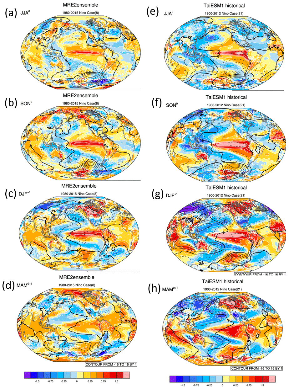
Figure 6The surface temperature (color shading) and SLP (contours; contour interval is 1 hPa; contours smaller than zero are dashed) of the El Niño composite in (a, e) JJA0, (b, f) SON0, (c, g) DJF+1, and (d, h) MAM+1 based on the MRE2 ensemble (left column) and TaiESM1 historical run (right column).
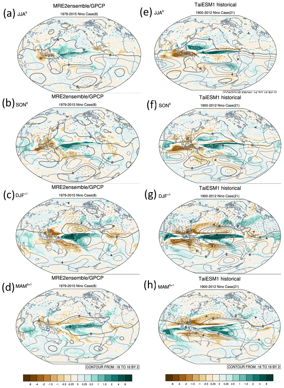
Figure 7As in Fig. 6 but showing precipitation (mm d−1; color shading) and 300 hPa stream function (contours; contour interval of 2 × 10⁶ m2 s−1 anomalies; contour values smaller than zero are dashed).
Figure 8 shows the seasonal evolution of ocean subsurface potential temperature averaged over the selected El Niño events. The composites show four seasonal means from JJA0 when an El Niño event was identified to MAM+1 in the following year. The green line shows the location of the 20 ∘C subsurface isotherm (Z20) during El Niño events, and the gray line shows the climatological Z20. During JJA0 in the observations, Z20 deepens in the eastern Pacific and shallows in the western Pacific (Fig. 8a). While TaiESM1 realistically simulated the climatological Z20 depth, it overestimated the response of subsurface temperatures and simulated a flatter Z20 profile in JJA0 (Fig. 8e). Such an overestimation bias in TaiESM1 continues from the beginning of the ENSO evolution through SON0 and DJF+1 (Fig. 8b, c, f, and g). Accompanied by the warm bias over the eastern Pacific, the cold bias developed in SON0 when the cool water started to form in the tropical western Pacific (Fig. 8b–d, f–h). Such a zonal dipole of subsurface temperature bias in TaiESM1 manifests a basin-wide response of ocean circulations during El Niño events. Moreover, both warming and cooling from the surface to 100 m depth were much more pronounced in the model than in the observation, especially over the eastern Pacific. An unrealistic warming in the central-eastern equatorial Pacific is also notable, reflecting the unrealistic westward extension of positive SSTA. This bias led to an anomalously strong SST gradient up to 2 ∘C between 180 and 150∘ W, consistent with the widespread strong westerly anomalies. In the meantime, the composite of subsurface zonal currents corresponding to El Niño events simulated in TaiESM1 is shown in Fig. S3. A strong westerly current anomaly suggests that zonal advection may also play a role in driving strong El Niño (Fig. S3). More analysis is needed to determine which model components are more responsible for these biases.
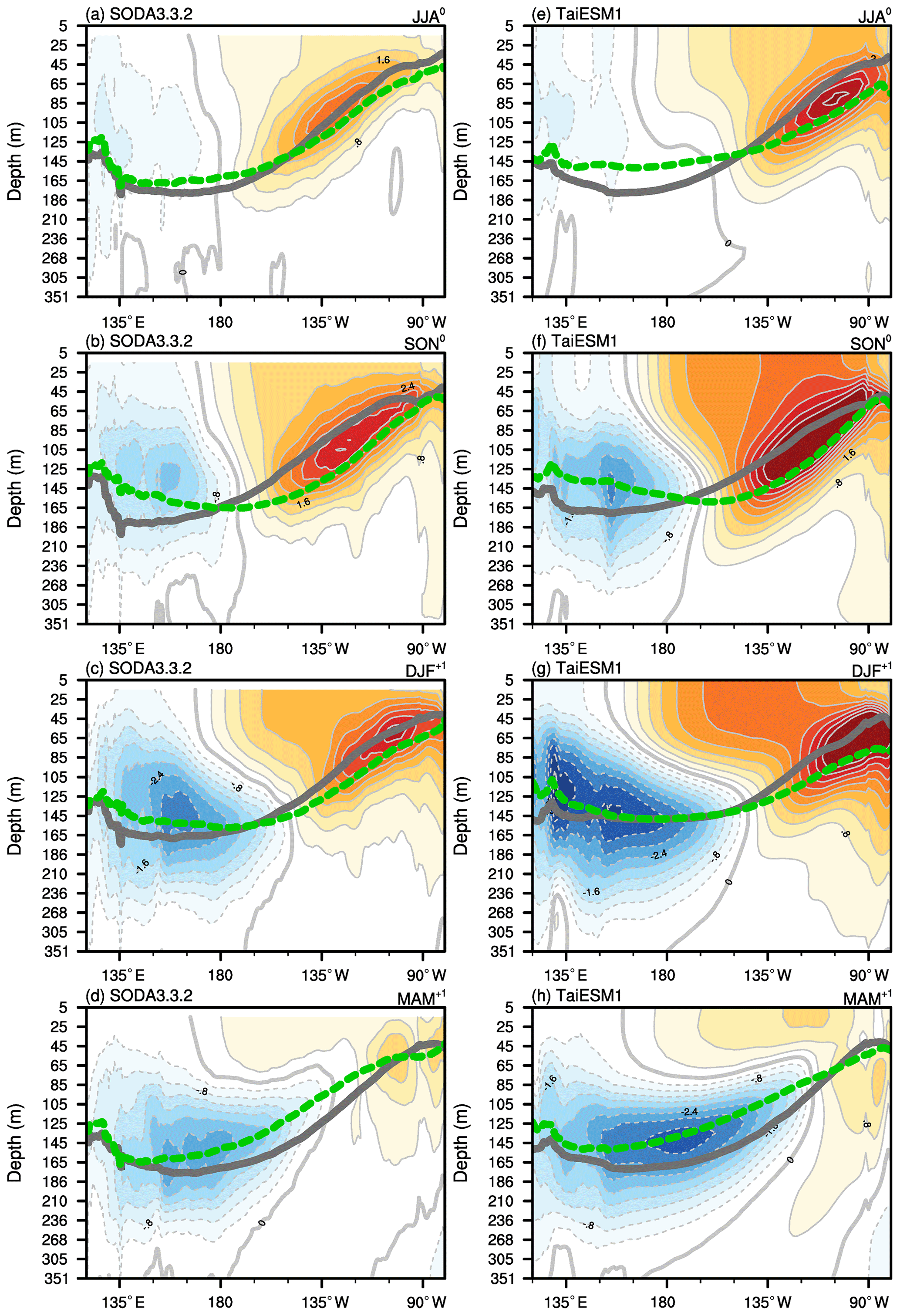
Figure 8Equatorial cross-section (5∘ S–5∘ N) of the El Niño composite of the potential temperature anomaly (color shading) in (a, e) JJA0, (b, f) SON0, (c, g) DJF+1, and (d, h) MAM+1 based on SODA v3.3.2 (left column) and the TaiESM1 historical run (right column). The gray line shows the climatological 20 ∘C isotherm (Z20), and the green dashed line shows the Z20 in the Niño state.
3.4 ENSO diversity and teleconnection
Based on the EP and CP events identified by the Niño 3–Niño 4 approach, we make longitudinal profiles of SSTA for both EP events and CP events simulated in TaiESM1 compared to observations (Fig. S4a). Our analysis reveals that TaiESM1 generally exhibits warmer SSTA over the tropical Pacific, particularly east of the 150∘ E line. Notably, during EP events, the model shows SSTA that can be as high as 1 ∘C over the eastern Pacific region. To further analyze the impacts of EP and CP events, we constructed composites of surface temperature and SLP based on four EP events and four CP events during the observation period (1980–2014), as well as CP and EP events during the historical TaiESM1 period (1900–2014).
Regarding the EP composite, TaiESM1 successfully captures the observed features over the tropical Pacific, as illustrated in Fig. S4b and c. However, the CP events identified in TaiESM1 exhibit elongated warm SSTA in the tropical region but with weaker teleconnections to the midlatitudes in the Northern Hemisphere (Fig. S4d and e). Additionally, the warming over North America is less pronounced and retreats towards the polar region in TaiESM1, whereas the observed cold surface temperature anomaly is replaced by a warm anomaly. These discrepancies suggest that biases in the model's mean state contribute to the model's biases in ENSO diversity and teleconnection patterns observed in TaiESM1, a common issue seen in other climate models as well (Ham and Kug, 2012).
In this section, we analyze the seasonal life cycle of the strong ENSO signals simulated in TaiESM1 to understand the intense tropical warming anomaly of El Niño events and link this bias with seasonal mean states. Based on the El Niño events defined in the previous section, we construct the seasonal cycle of El Niño events by plotting a Hovmöller diagram averaged over the Equator between 3∘ S and 3∘ N.
Figure 9 shows the Hovmöller diagram of SST anomalies and 1000 hPa zonal winds along the Equator (3∘ S–3∘ N) based on the strong El Niño event selected from the ERSSTv5 and TaiESM1 historical run. In the observation in May, the warm SSTA occurs over the dateline and the westerly wind anomaly starts to propagate to 135∘ W. In JJA0, the warm SST slowly develops at 180–135∘ W, progressively propagates to the eastern equatorial Pacific with westerly anomalies, and reaches maximum amplitude in November, December, and January (Fig. 9a). In contrast, the warm SST when initiated in May intensifies almost simultaneously in the basin east of 150∘ W in TaiESM1 (Fig. 9b). The warm anomaly quickly reaches 2 ∘C over the entire eastern equatorial Pacific through JJA0 and into September. Such warming seems to be coupled, with one branch quickly extending to the eastern equatorial Pacific after the initiation in May, whereas the westerly anomaly's major branch is well coupled with SSTA over the western Pacific most of the time. The warming continued developing even when the westerly anomalies in the eastern equatorial Pacific weakened in JJA0 and reached a maximum in January as in observations. This early development of a warm SSTA in the eastern equatorial Pacific in May and continuous warming in JJA0 and SON0 are two primary model biases that may contribute to strong El Niño events in TaiESM1.
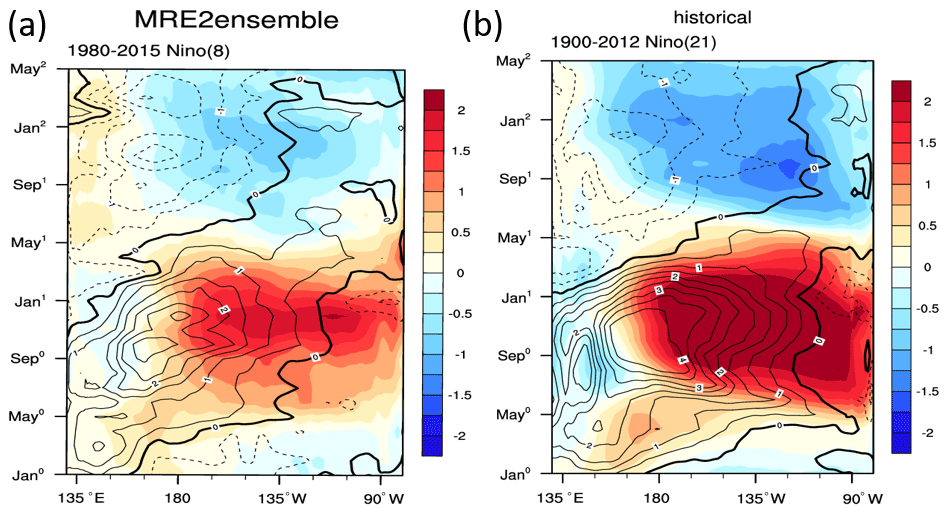
Figure 9Hovmöller diagram of composite SST anomalies (color) and zonal wind at 1000 hPa (contour) along the Equator (3∘ S–3∘ N) for El Niño based on (a) observations (ERSST–MRE2 ensemble from 1980 to 2015) and (b) the TaiESM1 historical run (1900–2014).
To understand the heat flux–SST coupling, we examined similar composites of net surface heat flux (Fig. S5a, b) and latent heat fluxes (Fig. S5c, d), which are the two heat fluxes prominent in observational El Niño events. Notably, in the observations, the seasonal variation of surface net heat fluxes in MRE2 is primarily controlled by latent heat fluxes, especially from May to November, as other heat fluxes play a minor role (Fig. S5c, d). However, the spatial patterns of net surface fluxes of TaiESM1 are primarily dominated by shortwave surface fluxes (Fig. S5d) and amplified by latent heat fluxes (Fig. 2b). Figure 10 shows the same Hovmöller diagram but for downwelling surface shortwave flux (color shading) and surface temperature (contours) composited over the El Niño events. Evolutions of shortwave radiation and SST during the life cycle of El Niño events in observations and TaiESM1 are shown in Fig. 10a and b, respectively. In the observations, upward shortwave fluxes of about 10 to 20 W m−2 (i.e., shown as negative in Fig. 10) are seen during the entire El Niño period, which is well collocated with the warm SSTA, due to the increased shortwave reflection of deep convection triggered by warmer SST. Such reflection of shortwave fluxes by deep clouds induces negative feedback (i.e., higher SST, large reflected shortwave radiation) between shortwave radiation flux and SST in the tropics (Fig. 10a). The negative feedback intensified in September, reached the maximum in December, and continued into the following February (Fig. 10a). In contrast to the observations, TaiESM1 produced unrealistically strong negative feedback over the western equatorial Pacific and Intertropical Convergence Zone (ITCZ) regions (Fig. 10b), as well as very strong positive shortwave radiation anomalies near the equatorial eastern Pacific after May in year 0 (Fig. 10a). The increase in shortwave influx starts from the eastern Pacific in May and gradually extends to 125∘ W in November, a feature that was not seen in observations. The westward progression of shortwave radiation increase contributes to erroneously strong SST warming, and its westward extension is seen in TaiESM1 from May to Jan in year 1 (Fig. 10b) instead of the observed simultaneous warming in the eastern Pacific.
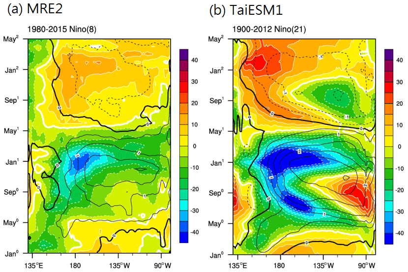
Figure 10A composite of El Niño events for RSDS (W m−2; color) and surface temperature (∘C; contour) in (a) MRE2 and (b) TaiESM1. Both variables are averaged over the Equator (3∘ S–3∘ N).
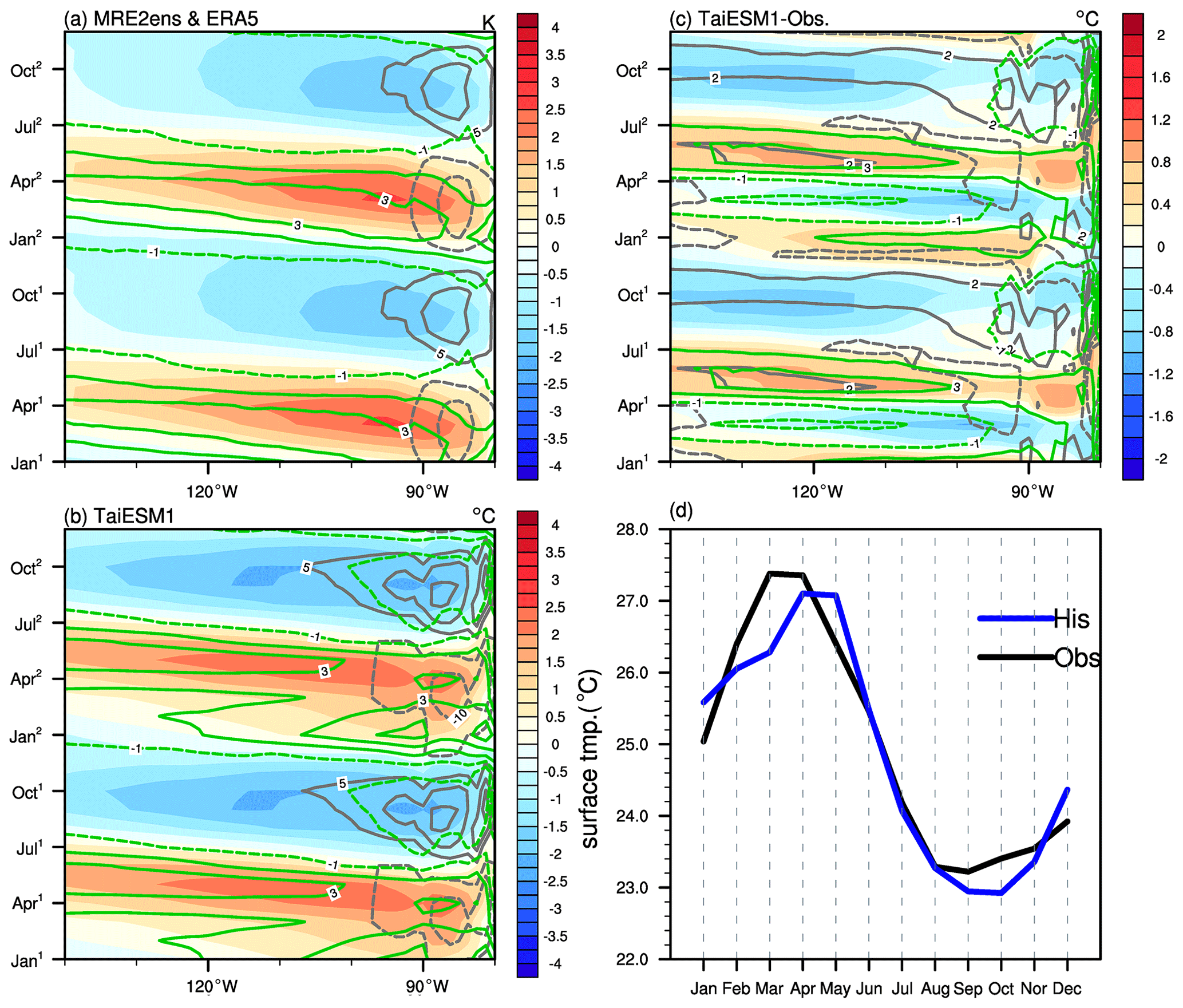
Figure 11Climatological seasonal cycle of the surface temperature (shaded area; ∘C), low clouds (gray contours; %), and 500 hPa vertical velocity (green contours; hPa s−1) for the tropical Pacific (3∘ S–3∘ N) in the (a) MRE2 ensemble and (b) TaiESM1, as well as (c) their differences. (d) The seasonal cycle of surface temperature at 100∘ W in MRE2 (black) and TaiESM1 (blue).
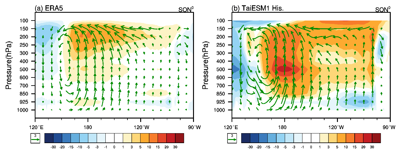
Figure 12Longitudinal height cross-section of the El Niño composite of September, October, and November in year 0 (SON0) along the Equator (5∘ S–5∘ N) based on (a) ERA5 and (b) TaiESM1. The cloud fraction (%) of the El Niño composite is shown in color shading, and the zonal and vertical winds (units: hPa s−1) are shown as green vectors.
To understand the cause of the strong SSTA development from May to November identified in Fig. 9 and its relationship with shortwave radiation fluxes in Fig. 10, we analyzed the seasonal cycle of low clouds (gray contours), vertical velocity (green contours), and SST (color shading) in the observations and TaiESM1 in Fig. 11a and b. Figure 11c shows the differences between TaiESM1 and MRE2. Figure 11d shows the climatological seasonal SST cycle at 100∘ W to show the SST differences where cloud biases are prominent. On the seasonal timescale in observations, the SSTA is closely coupled with anomalies of vertical velocity and low-level clouds. Cold surface temperature is commonly collocated with excessive low-level clouds and subsidence (Fig. 11a). While TaiESM1 also exhibits a clear seasonal variation like the observations in the eastern tropical Pacific (Fig. 11b), the simulated seasonal cycle is rather asymmetric with a colder bias during MAM0 and SON0 and warm biases during JJA0 and DJF+1 (Fig. 11c). Compared with the observations, TaiESM1 warmed approximately 1 month later during MAM0 and cooled deeper over the eastern Pacific in SON0 (Fig. 11c). The warmer MAM0 sea surface in TaiESM1 provides a smaller zonal SST gradient and may lead to the earlier onset of the eastward-propagating westerly anomaly found in MAM0 through the Bjerknes feedback (Fig. 9b). However, this cold surface temperature bias during SON0 provides a cold lower boundary for low stratus clouds to develop, leading to an environment for the strong positive feedback between shortwave fluxes and SST during El Niño events. Such impacts of the cold tongue bias are also found in CESM1 and CESM2, which share the same ocean model (i.e., POP2) as TaiESM1 (Y. C. Wang et al., 2015; Wei et al., 2021).
For a further look into the bias in SON0, Fig. 12 shows the changes in cloud fraction and zonal circulations in SON0 during the composited El Niño events. TaiESM1 successfully reproduced the eastward shift of the upward branch related to deep convection in response to the warm SST during El Niño events (Fig. 12a, b). However, TaiESM1 produced a much stronger response in circulations and cloud cover than the observations (Fig. 12b). Especially over the eastern Pacific, a stronger upward motion anomaly occurs and about 10 %–20 % of low clouds are reduced in TaiESM1, indicating a dramatic reduction of the low-cloud regime (Fig. 11c). As a result, more shortwave heat influxes are allowed into the ocean surface in SON0 when El Niño events occur (Fig. 10b). Consistent with the seasonal variation of SSTA in Fig. 9b, the increased shortwave fluxes thus help to keep the warm SSTA in SON0 over the eastern Pacific after the warm SSTA initiates in MAM0 in TaiESM1 (Fig. 10b).
This study documented ENSO's fundamental statistics and features in TaiESM1, a CMIP6 participant. Compared with the observational dataset, TaiESM1 has captured many prominent observed ENSO features, including a 3–5-year spectrum peak, seasonal phasing, the evolution of warm SST, deepening of the subsurface layer during an El Niño event, and teleconnection patterns in midlatitudes. However, the simulated El Niño signals in TaiESM1 are much stronger and more prolonged than the observed ENSO signals. Such strong signals are shown as intense warm SSTA over the tropical Pacific within the spatial structure of the composite of the El Niño event. In the meantime, in response to the tropical warm SSTA, the teleconnection wave activities associated with El Niño events are much stronger in TaiESM1, significantly affecting temperature and rainfall in high-latitude regions, although with a similar spatial pattern to the observations.
To understand the cause of the warm El Niño biases, we investigated the seasonal cycle of strong El Niño events in TaiESM1. Compared with the observed delay of SST propagation to the central Pacific in May after the wind anomaly's initiation, the simulated SST warming quickly propagates toward the eastern Pacific along with the westerly wind anomaly in TaiESM1. The SST warming continued through November and reached a maximum in December, showing a stronger and more prolonged warm period than the observation. Moreover, in contrast to the negative feedback found in observations, our analysis shows that the strong El Niño warm anomalies in TaiESM1 is due to the strong SST–heat flux positive feedbacks, especially over the eastern Pacific in SON0. Further analysis shows that this biased feedback is due to the response of the spurious low-cloud regime off the west coast of South America simulated in TaiESM1. This biased cloud regime results from the seasonal variation of the cold tongue over the eastern Pacific, consistent with previous studies using the CESM family and CMIP models (Ham and Kug, 2012; Wei et al., 2021). During El Niño events, the stratus clouds over the eastern Pacific gradually diminished due to the warmer SST, allowing solar radiation to warm the ocean surface. This result leads to a positive feedback of downward solar radiation and SST over the eastern Pacific, an opposite sign of the observed relationship. This biased relationship is typical in the CMIP5 and CMIP6 models (Bayr et al., 2019; Beobide-Arsuaga et al., 2021).
In summary, TaiESM1 can reproduce many fundamental features of ENSO. However, it still possesses several biases shared by other CMIP6 models, including the lack of randomness of El Niño events, El Niño magnitudes that are too strong, and early SST warming in the early stage of El Niño events. The strong El Niño strength, our analysis found, mainly results from the biased atmosphere–SST coupling accompanied by biases of the mean state and seasonal cycle of the cold tongue and Walker circulation, which is consistent with previous studies with CMIP5 and/or CMIP6 models (Bayr et al., 2018; Chen et al., 2021). However, to resolve this bias (and others), more detailed analysis, including process-related metrics, and more model experiments, such as atmosphere-only and ocean-only experiments, are required to determine the cause and effects of the observed biases. For TaiESM1, we plan to implement ocean-only experiments with the ocean component POP2, allowing us to quantify the ocean's response to biased winds and radiation fluxes. We will also conduct AMIP-type simulations to investigate the development of westerly wind anomalies under biased SST conditions. Combined with process-oriented diagnosis, these model experiments will help us to determine and better comprehend the causes and effects of these observed biases. Also echoed with other studies of ENSO evaluations of CMIP6, our analysis suggests that a more process-based development strategy focusing on atmosphere–ocean coupling rather than a feature-based evaluation of ENSO is needed to reduce the uncertainty of ENSO simulations and future ENSO projection in climate models.
All observational and analysis datasets used in this study are available online. The MRE2 ensemble can be downloaded from the website of the Collaborative REAnalysis Technical Environment – Intercomparison Project (https://esgf-node.llnl.gov/projects/create-ip/data_description, CREATE-IP Project, 2018). The ERA5 monthly data can be downloaded from the Copernicus Climate Change Service Climate Data Store (DOI: https://doi.org/10.24381/cds.f17050d7, Hersbach et al., 2023a; DOI: https://doi.org/10.24381/cds.6860a573, Hersbach et al., 2023b). The data from the Simple Ocean Data Assimilation (SODA) v3.3.2 can be downloaded from the SODA website (https://www2.atmos.umd.edu/~ocean/index_files/soda3.3.2_mn_download_b.htm, SODA project, 2018). The Global Precipitation Climatology Project version 2.3 and Extended Reconstructed Sea Surface Temperature version 5 can be downloaded from the website of the NOAA PSL, Boulder, Colorado, USA (https://psl.noaa.gov/data/gridded/data.gpcp.html, GPCP, 2009 and https://doi.org/10.7289/V5T72FNM, Huang et al., 2018). The model code of TaiESM version 1 is available at https://doi.org/10.5281/zenodo.3626654 (rceclccr, 2020). All post-processing codes to produce figures presented in this paper are available at https://doi.org/10.5281/zenodo.7740033 (Chen, 2023). The description and data for historical simulations of TaiESM1 can be found at https://doi.org/10.22033/ESGF/CMIP6.9755 (Lee and Liang, 2020).
The supplement related to this article is available online at: https://doi.org/10.5194/gmd-16-4599-2023-supplement.
YCW, WLT: methodology, investigation, writing – original draft, review, and editing. YLC: software, formal analysis, visualization. SYL: conceptualization, investigation, writing – review and editing HHH: conceptualization, methodology, writing – review and editing, supervision. HCL: data curation.
The contact author has declared that none of the authors has any competing interests.
Publisher's note: Copernicus Publications remains neutral with regard to jurisdictional claims in published maps and institutional affiliations.
We would like to express our gratitude to the National Center for High-Performance Computing, Taiwan, for providing the facilities for the CMIP6 participation of TaiESM1. We wish to express our appreciation to the two reviewers for their insightful comments, which have played a crucial role in enhancing this paper.
This research has been supported by the Taiwan National Science and Technology Council (grant nos. MOST 111-2111-M-001-013, MOST 111-2111-M-002-020, and MOST 110-2123-M-001-003).
This paper was edited by Riccardo Farneti and reviewed by Michael J. McPhaden and one anonymous referee.
Adler, R. F., Huffman, G. J., Chang, A., Ferraro, R., Xie, P.-P., Janowiak, J., Rudolf, B., Schneider, U., Curtis, S., Bolvin, D., Gruber, A., Susskind, J., Arkin, P., and Nelkin, E.: The Version-2 Global Precipitation Climatology Project (GPCP) Monthly Precipitation Analysis (1979–Present), J. Hydrometeorol., 4, 1147–1167, https://doi.org/10.1175/1525-7541(2003)004<1147:TVGPCP>2.0.CO;2, 2003.
Bayr, T., Latif, M., Dommenget, D., Wengel, C., Harlaß, J., and Park, W.: Mean-state dependence of ENSO atmospheric feedbacks in climate models, Clim. Dynam., 50, 3171–3194, https://doi.org/10.1007/s00382-017-3799-2, 2018.
Bayr, T., Wengel, C., Latif, M., Dommenget, D., Lübbecke, J., and Park, W.: Error compensation of ENSO atmospheric feedbacks in climate models and its influence on simulated ENSO dynamics, Clim. Dynam., 53, 155–172, https://doi.org/10.1007/s00382-018-4575-7, 2019.
Bellenger, H., Guilyardi, E., Leloup, J., Lengaigne, M., and Vialard, J.: ENSO representation in climate models: from CMIP3 to CMIP5, Clim. Dynam., 42, 1999–2018, https://doi.org/10.1007/s00382-013-1783-z, 2014.
Beobide-Arsuaga, G., Bayr, T., Reintges, A., and Latif, M.: Uncertainty of ENSO-amplitude projections in CMIP5 and CMIP6 models, Clim. Dynam., 56, 3875–3888, https://doi.org/10.1007/s00382-021-05673-4, 2021.
Bjerknes, J.: Atmospheric Teleconnections from the Equatorial Pacific, Mon. Weather Rev., 97, 163–172, https://doi.org/10.1175/1520-0493(1969)097<0163:ATFTEP>2.3.CO;2, 1969.
Cane, M. A.: The evolution of El Niño, past and future, Earth Planet. Sc. Lett., 230, 227–240, https://doi.org/10.1016/j.epsl.2004.12.003, 2005.
Capotondi, A., Deser, C., Phillips, A. S., Okumura, Y., and Larson, S. M.: ENSO and Pacific Decadal Variability in the Community Earth System Model Version 2, J. Adv. Model. Earth Sy., 12, e2019MS002022, https://doi.org/10.1029/2019MS002022, 2020a.
Capotondi, A., Wittenberg, A. T., Kug, J., Takahashi, K., and McPhaden, M. J.: ENSO Diversity, in: El Niño Southern Oscillation in a Changing Climate, 65–86, https://doi.org/10.1002/9781119548164.ch4, 2020b.
Carton, J. A., Chepurin, G. A., and Chen, L.: SODA3: A New Ocean Climate Reanalysis, J. Climate, 31, 6967–6983, https://doi.org/10.1175/JCLI-D-18-0149.1, 2018.
Chen, C., Cane, M. A., Wittenberg, A. T., and Chen, D.: ENSO in the CMIP5 Simulations: Life Cycles, Diversity, and Responses to Climate Change, J. Climate, 30, 775–801, https://doi.org/10.1175/JCLI-D-15-0901.1, 2017.
Chen, C.-A., Hsu, H.-H., and Liang, H.-C.: Evaluation and comparison of CMIP6 and CMIP5 model performance in simulating the seasonal extreme precipitation in the Western North Pacific and East Asia, Weather Clim. Extrem., 31, 100303, https://doi.org/10.1016/j.wace.2021.100303, 2021.
Chen, H.-C. and Jin, F.-F.: Simulations of ENSO Phase-locking in CMIP5 and CMIP6, J. Climate, 34, 5135–5149, https://doi.org/10.1175/JCLI-D-20-0874.1, 2021.
Chen, J.-P., Tsai, I.-C., and Lin, Y.-C.: A statistical–numerical aerosol parameterization scheme, Atmos. Chem. Phys., 13, 10483–10504, https://doi.org/10.5194/acp-13-10483-2013, 2013.
Chen, Y.-L.: ENSO statistics, teleconnections, and atmosphere-ocean coupling in the Taiwan Earth System Model version 1 (Version 1), Zenodo [code], https://doi.org/10.5281/zenodo.7740033, 2023.
Compo, G. P., Whitaker, J. S., Sardeshmukh, P. D., Matsui, N., Allan, R. J., Yin, X., Gleason, B. E., Vose, R. S., Rutledge, G., Bessemoulin, P., Brönnimann, S., Brunet, M., Crouthamel, R. I., Grant, A. N., Groisman, P. Y., Jones, P. D., Kruk, M. C., Kruger, A. C., Marshall, G. J., Maugeri, M., Mok, H. Y., Nordli, Ø., Ross, T. F., Trigo, R. M., Wang, X. L., Woodruff, S. D., and Worley, S. J.: The Twentieth Century Reanalysis Project, Q. J. Roy. Meteor. Soc., 137, 1–28, https://doi.org/10.1002/qj.776, 2011.
CREATE-IP Project: Data Description, ESGF [data set], https://esgf-node.llnl.gov/projects/create-ip/data_description (last access: December 2019), 2018.
Dee, D. P., Uppala, S. M., Simmons, A. J., Berrisford, P., Poli, P., Kobayashi, S., Andrae, U., Balmaseda, M. A., Balsamo, G., Bauer, P., Bechtold, P., Beljaars, A. C. M., van de Berg, L., Bidlot, J., Bormann, N., Delsol, C., Dragani, R., Fuentes, M., Geer, A. J., Haimberger, L., Healy, S. B., Hersbach, H., Hólm, E. V., Isaksen, L., Kållberg, P., Köhler, M., Matricardi, M., McNally, A. P., Monge-Sanz, B. M., Morcrette, J.-J., Park, B.-K., Peubey, C., de Rosnay, P., Tavolato, C., Thépaut, J.-N., and Vitart, F.: The ERA-Interim reanalysis: configuration and performance of the data assimilation system, Q. J. Roy. Meteor. Soc., 137, 553–597, https://doi.org/10.1002/qj.828, 2011.
Diaz, H. F., Hoerling, M. P., and Eischeid, J. K.: ENSO variability, teleconnections and climate change, Int. J. Climatol., 21, 1845–1862, https://doi.org/10.1002/joc.631, 2001.
Fedorov, A. V., Hu, S., Wittenberg, A. T., Levine, A. F. Z., and Deser, C.: ENSO Low-Frequency Modulation and Mean State Interactions, in: El Niño Southern Oscillation in a Changing Climate, 173–198, https://doi.org/10.1002/9781119548164.ch8, 2020.
Gelaro, R., McCarty, W., Suárez, M. J., Todling, R., Molod, A., Takacs, L., Randles, C. A., Darmenov, A., Bosilovich, M. G., Reichle, R., Wargan, K., Coy, L., Cullather, R., Draper, C., Akella, S., Buchard, V., Conaty, A., da Silva, A. M., Gu, W., Kim, G.-K., Koster, R., Lucchesi, R., Merkova, D., Nielsen, J. E., Partyka, G., Pawson, S., Putman, W., Rienecker, M., Schubert, S. D., Sienkiewicz, M., and Zhao, B.: The Modern-Era Retrospective Analysis for Research and Applications, Version 2 (MERRA-2), J. Climate, 30, 5419–5454, https://doi.org/10.1175/JCLI-D-16-0758.1, 2017.
Glantz, M. H.: Currents of change: impacts of El Niño and La Niña on climate and society, Cambridge University Press, ISBN 9780521786720, 2001.
Global Precipitation Climatology Project (GPCP): Global Precipitation Climatology Project (GPCP) Monthly Analysis Product, NOAA [data set], https://psl.noaa.gov/data/gridded/data.gpcp.html (last access: June 2020), 2009.
Guilyardi, E., Wittenberg, A., Fedorov, A., Collins, M., Wang, C., Capotondi, A., van Oldenborgh, G. J., and Stockdale, T.: Understanding El Niño in Ocean–Atmosphere General Circulation Models: Progress and Challenges, B. Am. Meteorol. Soc., 90, 325–340, https://doi.org/10.1175/2008BAMS2387.1, 2009.
Guilyardi, E., Capotondi, A., Lengaigne, M., Thual, S., and Wittenberg, A. T.: ENSO Modeling: history, progress, and challenges, in: El Niño Southern Oscillation in a Changing Climate, edited by: McPhaden, M. J., Santoso, A., and Cai, W., American Geophsical Union, 199–226, https://doi.org/10.1002/9781119548164.ch9, 2020.
Ham, Y.-G. and Kug, J.-S.: How well do current climate models simulate two types of El Nino?, Clim. Dynam., 39, 383–398, https://doi.org/10.1007/s00382-011-1157-3, 2012.
Hersbach, H., Bell, B., Berrisford, P., Hirahara, S., Horányi, A., Muñoz-Sabater, J., Nicolas, J., Peubey, C., Radu, R., Schepers, D., Simmons, A., Soci, C., Abdalla, S., Abellan, X., Balsamo, G., Bechtold, P., Biavati, G., Bidlot, J., Bonavita, M., Chiara, G., Dahlgren, P., Dee, D., Diamantakis, M., Dragani, R., Flemming, J., Forbes, R., Fuentes, M., Geer, A., Haimberger, L., Healy, S., Hogan, R. J., Hólm, E., Janisková, M., Keeley, S., Laloyaux, P., Lopez, P., Lupu, C., Radnoti, G., Rosnay, P., Rozum, I., Vamborg, F., Villaume, S., and Thépaut, J.: The ERA5 global reanalysis, Q. J. Roy. Meteor. Soc., 146, 1999–2049, https://doi.org/10.1002/qj.3803, 2020.
Hersbach, H., Bell, B., Berrisford, P., Biavati, G., Horányi, A., Muñoz Sabater, J., Nicolas, J., Peubey, C., Radu, R., Rozum, I., Schepers, D., Simmons, A., Soci, C., Dee, D., and Thépaut, J.-N.: ERA5 monthly averaged data on single levels from 1940 to present, Copernicus Climate Change Service (C3S) Climate Data Store (CDS) [data set], https://doi.org/10.24381/cds.f17050d7, 2023a.
Hersbach, H., Bell, B., Berrisford, P., Biavati, G., Horányi, A., Muñoz Sabater, J., Nicolas, J., Peubey, C., Radu, R., Rozum, I., Schepers, D., Simmons, A., Soci, C., Dee, D., and Thépaut, J.-N.: ERA5 monthly averaged data on pressure levels from 1940 to present, Copernicus Climate Change Service (C3S) Climate Data Store (CDS) [data set], https://doi.org/10.24381/cds.6860a573, 2023b.
Huang, B., Thorne, P. W., Banzon, V. F., Boyer, T., Chepurin, G., Lawrimore, J. H., Menne, M. J., Smith, T. M., Vose, R. S., and Zhang, H.-M.: Extended Reconstructed Sea Surface Temperature, Version 5 (ERSSTv5): Upgrades, Validations, and Intercomparisons, J. Climate, 30, 8179–8205, https://doi.org/10.1175/JCLI-D-16-0836.1, 2017.
Huang, B., Thorne, P. W., Banzon, V. F., Boyer, T., Chepurin, G., Lawrimore, J. H., Menne, M. J., Smith, T. M., Vose, R. S., and Zhang, H.-M.: NOAA Extended Reconstructed Sea Surface Temperature (ERSST), Version 5, NOAA [data set], https://doi.org/10.7289/V5T72FNM, 2018.
Huffman, G. J., Adler, R. F., Bolvin, D. T., and Gu, G.: Improving the global precipitation record: GPCP Version 2.1, Geophys. Res. Lett., 36, L17808, https://doi.org/10.1029/2009GL040000, 2009.
Hurrell, J. W., Holland, M. M., Gent, P. R., Ghan, S., Kay, J. E., Kushner, P. J., Lamarque, J.-F., Large, W. G., Lawrence, D., Lindsay, K., Lipscomb, W. H., Long, M. C., Mahowald, N., Marsh, D. R., Neale, R. B., Rasch, P., Vavrus, S., Vertenstein, M., Bader, D., Collins, W. D., Hack, J. J., Kiehl, J., and Marshall, S.: The Community Earth System Model: A Framework for Collaborative Research, B. Am. Meteorol. Soc., 94, 1339–1360, https://doi.org/10.1175/BAMS-D-12-00121.1, 2013.
Jha, B., Hu, Z.-Z., and Kumar, A.: SST and ENSO variability and change simulated in historical experiments of CMIP5 models, Clim. Dynam., 42, 2113–2124, https://doi.org/10.1007/s00382-013-1803-z, 2014.
Jin, F.-F.: An Equatorial Ocean Recharge Paradigm for ENSO. Part I: Conceptual Model, J. Atmos. Sci., 54, 811–829, https://doi.org/10.1175/1520-0469(1997)054<0811:AEORPF>2.0.CO;2, 1997.
Kobayashi, S., Ota, Y., Harada, Y., Ebita, A., Moriya, M., Onoda, H., Onogi, K., Kamahori, H., Kobayashi, C., Endo, H., Miyaoka, K., and Takahashi, K.: The JRA-55 Reanalysis: General Specifications and Basic Characteristics, J. Meteorol. Soc. Jpn. Ser. II, 93, 5–48, https://doi.org/10.2151/jmsj.2015-001, 2015.
Kug, J.-S., Jin, F.-F., and An, S.-I.: Two Types of El Niño Events: Cold Tongue El Niño and Warm Pool El Niño, J. Climate, 22, 1499–1515, https://doi.org/10.1175/2008JCLI2624.1, 2009.
Kumar, A. and Hu, Z.-Z.: Uncertainty in the ocean–atmosphere feedbacks associated with ENSO in the reanalysis products, Clim. Dynam., 39, 575–588, https://doi.org/10.1007/s00382-011-1104-3, 2012.
Latif, M., Anderson, D., Barnett, T., Cane, M., Kleeman, R., Leetmaa, A., O'Brien, J., Rosati, A., and Schneider, E.: A review of the predictability and prediction of ENSO, J. Geophys. Res.-Oceans, 103, 14375–14393, https://doi.org/10.1029/97JC03413, 1998.
Lee, W.-L. and Liang, H.-C.: AS-RCEC TaiESM1.0 model output prepared for CMIP6 CMIP historical, Version 20200623[1], Earth System Grid Federation [data set], https://doi.org/10.22033/ESGF/CMIP6.9755, 2020.
Lee, W.-L., Liou, K. N., and Wang, C.: Impact of 3-D topography on surface radiation budget over the Tibetan Plateau, Theor. Appl. Climatol., 113, 95–103, https://doi.org/10.1007/s00704-012-0767-y, 2013.
Lee, W.-L., Wang, Y.-C., Shiu, C.-J., Tsai, I., Tu, C.-Y., Lan, Y.-Y., Chen, J.-P., Pan, H.-L., and Hsu, H.-H.: Taiwan Earth System Model Version 1: description and evaluation of mean state, Geosci. Model Dev., 13, 3887–3904, https://doi.org/10.5194/gmd-13-3887-2020, 2020.
Lloyd, J., Guilyardi, E., Weller, H., and Slingo, J.: The role of atmosphere feedbacks during ENSO in the CMIP3 models, Atmos. Sci. Lett., 10, 170–176, https://doi.org/10.1002/asl.227, 2009.
Lloyd, J., Guilyardi, E., and Weller, H.: The role of atmosphere feedbacks during ENSO in the CMIP3 models. Part II: using AMIP runs to understand the heat flux feedback mechanisms, Clim. Dynam., 37, 1271–1292, https://doi.org/10.1007/s00382-010-0895-y, 2011.
McPhaden, M. J., Busalacchi, A. J., Cheney, R., Donguy, J.-R., Gage, K. S., Halpern, D., Ji, M., Julian, P., Meyers, G., Mitchum, G. T., Niiler, P. P., Picaut, J., Reynolds, R. W., Smith, N., and Takeuchi, K.: The Tropical Ocean-Global Atmosphere observing system: A decade of progress, J. Geophys. Res.-Oceans, 103, 14169–14240, https://doi.org/10.1029/97JC02906, 1998.
McPhaden, M. J., Zebiak, S. E., and Glantz, M. H.: ENSO as an Integrating Concept in Earth Science, Science, 314, 1740–1745, https://doi.org/10.1126/science.1132588, 2006.
McPhaden, M. J., Lee, T., and McClurg, D.: El Niño and its relationship to changing background conditions in the tropical Pacific Ocean, Geophys. Res. Lett., 38, L15709, https://doi.org/10.1029/2011GL048275, 2011.
Neelin, J. D., Battisti, D. S., Hirst, A. C., Jin, F.-F., Wakata, Y., Yamagata, T., and Zebiak, S. E.: ENSO theory, J. Geophys. Res.-Oceans, 103, 14261–14290, https://doi.org/10.1029/97JC03424, 1998.
NOAA Climate Prediction Center: Historical El Nino/La Nina episodes (1950–present), NOAA [data set], https://www.cpc.ncep.noaa.gov/products/analysis_monitoring/ensostuff/ensoyears_1971-2000_climo.shtml (last access: December 2020), 2000.
Onogi, K., Tsutsui, J., Koide, H., Sakamoto, M., Kobayashi, S., Hatsushika, H., Matsumoto, T., Yamazaki, N., Kamahori, H., Takahashi, K., Kadokura, S., Wada, K., Kato, K., Oyama, R., Ose, T., Mannoji, N., and Taira, R.: The JRA-25 Reanalysis, J. Meteorol. Soc. Jpn. Ser. II, 85, 369–432, https://doi.org/10.2151/jmsj.85.369, 2007.
Park, J., Kim, H., Simon Wang, S.-Y., Jeong, J.-H., Lim, K.-S., LaPlante, M., and Yoon, J.-H.: Intensification of the East Asian summer monsoon lifecycle based on observation and CMIP6, Environ. Res. Lett., 15, 0940b9, https://doi.org/10.1088/1748-9326/ab9b3f, 2020.
Philander, S.: El Nino, La Nina, and the Southern Oscillation, edited by: Philander, S. G., Academic Press, 1–293, ISBN 9780080570983, 1989.
Planton, Y. Y., Guilyardi, E., Wittenberg, A. T., Lee, J., Gleckler, P. J., Bayr, T., McGregor, S., McPhaden, M. J., Power, S., Roehrig, R., Vialard, J., and Voldoire, A.: Evaluating Climate Models with the CLIVAR 2020 ENSO Metrics Package, B. Am. Meteorol. Soc., 102, E193–E217, https://doi.org/10.1175/BAMS-D-19-0337.1, 2021.
Potter, G. L., Carriere, L., Hertz, J., Bosilovich, M., Duffy, D., Lee, T., and Williams, D. N.: Enabling Reanalysis Research Using the Collaborative Reanalysis Technical Environment (CREATE), B. Am. Meteorol. Soc., 99, 677–687, https://doi.org/10.1175/BAMS-D-17-0174.1, 2018.
rceclccr: rceclccr/TaiESM v1.0.0 (v1.0.0), Zenodo [code], https://doi.org/10.5281/zenodo.3626654, 2020.
Rienecker, M. M., Suarez, M. J., Gelaro, R., Todling, R., Bacmeister, J., Liu, E., Bosilovich, M. G., Schubert, S. D., Takacs, L., Kim, G.-K., Bloom, S., Chen, J., Collins, D., Conaty, A., da Silva, A., Gu, W., Joiner, J., Koster, R. D., Lucchesi, R., Molod, A., Owens, T., Pawson, S., Pegion, P., Redder, C. R., Reichle, R., Robertson, F. R., Ruddick, A. G., Sienkiewicz, M., and Woollen, J.: MERRA: NASA's Modern-Era Retrospective Analysis for Research and Applications, J. Climate, 24, 3624–3648, https://doi.org/10.1175/JCLI-D-11-00015.1, 2011.
Saha, S., Moorthi, S., Pan, H.-L., Wu, X., Wang, J., Nadiga, S., Tripp, P., Kistler, R., Woollen, J., Behringer, D., Liu, H., Stokes, D., Grumbine, R., Gayno, G., Wang, J., Hou, Y.-T., Chuang, H., Juang, H.-M. H., Sela, J., Iredell, M., Treadon, R., Kleist, D., Van Delst, P., Keyser, D., Derber, J., Ek, M., Meng, J., Wei, H., Yang, R., Lord, S., van den Dool, H., Kumar, A., Wang, W., Long, C., Chelliah, M., Xue, Y., Huang, B., Schemm, J.-K., Ebisuzaki, W., Lin, R., Xie, P., Chen, M., Zhou, S., Higgins, W., Zou, C.-Z., Liu, Q., Chen, Y., Han, Y., Cucurull, L., Reynolds, R. W., Rutledge, G., and Goldberg, M.: The NCEP Climate Forecast System Reanalysis, B. Am. Meteorol. Soc., 91, 1015–1058, https://doi.org/10.1175/2010BAMS3001.1, 2010.
Shiu, C.-J., Wang, Y.-C., Hsu, H.-H., Chen, W.-T., Pan, H.-L., Sun, R., Chen, Y.-H., and Chen, C.-A.: GTS v1.0: a macrophysics scheme for climate models based on a probability density function, Geosci. Model Dev., 14, 177–204, https://doi.org/10.5194/gmd-14-177-2021, 2021.
Simple Ocean Data Assimilation (SODA) project: SODA3.3.2 download page, SODA [data set], https://www2.atmos.umd.edu/~ocean/index_files/soda3.3.2_mn_download_b.htm (last access: March 2023), 2018.
Smith, R., Jones, P., Briegleb, B., Bryan, F., Danabasoglu, G., Dennis, J., Dukowicz, J., Fox-Kemper, B., Eden, C., Gent, P., Hecht, M., Jayne, S., Jochum, M., Large, W., Lindsay, K., Maltrud, M., Norton, N., Peacock, S., Vertenstein, M., and Yeager, S.: The Parallel Ocean Program (POP) Reference Manual: : Ocean component of the community climate system model, Los Alamos National Laboratory Tech. Rep. LAUR-10-01853, 2010.
Wang, C.: A review of ENSO theories, Natl. Sci. Rev., 5, 813–825, https://doi.org/10.1093/nsr/nwy104, 2018.
Wang, C. and Picaut, J.: Understanding Enso Physics-A Review, in: Earth's Climate: The Ocean-Atmosphere Interaction, edited by: Wang, C., Xie, S.-P., and Carton, J. A., American Geophysical Union, 21–48, https://doi.org/10.1029/147GM02, 2013.
Wang, C.-C., Lee, W.-L., Chen, Y.-L., and Hsu, H.-H.: Processes Leading to Double Intertropical Convergence Zone Bias in CESM1/CAM5, J. Climate, 28, 2900–2915, https://doi.org/10.1175/JCLI-D-14-00622.1, 2015.
Wang, Y., Hsu, H., Chen, C., Tseng, W., Hsu, P., Lin, C., Chen, Y., Jiang, L., Lee, Y., Liang, H., Chang, W., Lee, W., and Shiu, C.: Performance of the Taiwan Earth System Model in Simulating Climate Variability Compared With Observations and CMIP6 Model Simulations, J. Adv. Model. Earth Sy., 13, e2020MS002353, https://doi.org/10.1029/2020MS002353, 2021.
Wang, Y.-C., Pan, H. L., and Hsu, H. H.: Impacts of the triggering function of cumulus parameterization on warm-season diurnal rainfall cycles at the Atmospheric Radiation Measurement Southern Great Plains Site, J. Geophys. Res., 120, 10681–10702, https://doi.org/10.1002/2015JD023337, 2015.
Wei, H., Subramanian, A. C., Karnauskas, K. B., DeMott, C. A., Mazloff, M. R., and Balmaseda, M. A.: Tropical Pacific Air-Sea Interaction Processes and Biases in CESM2 and Their Relation to El Niño Development, J. Geophys. Res.-Oceans, 126, 185–206, https://doi.org/10.1029/2020JC016967, 2021.
Yeh, S.-W., Cai, W., Min, S.-K., McPhaden, M. J., Dommenget, D., Dewitte, B., Collins, M., Ashok, K., An, S.-I., Yim, B.-Y., and Kug, J.-S.: ENSO Atmospheric Teleconnections and Their Response to Greenhouse Gas Forcing, Rev. Geophys., 56, 185–206, https://doi.org/10.1002/2017RG000568, 2018.
Zhao, B. and Fedorov, A.: The Effects of Background Zonal and Meridional Winds on ENSO in a Coupled GCM, J. Climate, 33, 2075–2091, https://doi.org/10.1175/JCLI-D-18-0822.1, 2020.
- Abstract
- Introduction
- Data, models, and methodology
- Basic statistics of ENSO in TaiESM1
- Linking the warm SST bias during El Niño events with simulated seasonal mean states
- Summary
- Code and data availability
- Author contributions
- Competing interests
- Disclaimer
- Acknowledgements
- Financial support
- Review statement
- References
- Supplement