the Creative Commons Attribution 4.0 License.
the Creative Commons Attribution 4.0 License.
 | 28 Jul 2023
TIMBER v0.1: a conceptual framework for emulating temperature responses to tree cover change
Shruti Nath
Lukas Gudmundsson
Jonas Schwaab
Gregory Duveiller
Steven J. De Hertog
Felix Havermann
Iris Manola
Julia Pongratz
Sonia I. Seneviratne
Carl F. Schleussner
Wim Thiery
Quentin Lejeune
Land cover changes have been proposed to play a significant role, alongside emission reductions, in achieving the temperature goals agreed upon under the Paris Agreement. Such changes carry both global implications, pertaining to the biogeochemical effects of land cover change and thus the global carbon budget, and regional or local implications, pertaining to the biogeophysical effects arising within the immediate area of land cover change. Biogeophysical effects of land cover change are of high relevance to national policy and decision makers, and accounting for them is essential for effective deployment of land cover practices that optimise between global and regional impacts. To this end, Earth system model (ESM) outputs that isolate the biogeophysical responses of climate to land cover changes are key in informing impact assessments and supporting scenario development exercises. However, generating multiple such ESM outputs in a manner that allows comprehensive exploration of all plausible land cover scenarios is computationally untenable. This study proposes a framework to explore in an agile manner the local biogeophysical responses of climate under customised tree cover change scenarios by means of a computationally inexpensive emulator, the Tree cover change clIMate Biophysical responses EmulatoR (TIMBER) v0.1. The emulator is novel in that it solely represents the biogeophysical responses of climate to tree cover changes, and it can be used as either a standalone device or as a supplement to existing climate model emulators that represent the climate responses from greenhouse gas (GHG) or global mean temperature (GMT) forcings. We start off by modelling local minimum, mean, and maximum surface temperature responses to tree cover changes by means of a month- and Earth system model (ESM)-specific generalised additive model (GAM) trained over the whole globe; 2 m air temperature responses are then diagnosed from the modelled minimum and maximum surface temperature responses using observationally derived relationships. Such a two-step procedure accounts for the different physical representations of surface temperature responses to tree cover changes under different ESMs whilst respecting a definition of 2 m air temperature that is more consistent across ESMs and with observational datasets. In exploring new tree cover change scenarios, we employ a parametric bootstrap sampling method to generate multiple possible temperature responses, such that the parametric uncertainty within the GAM is also quantified. The output of the final emulator is demonstrated for the Shared Socioeconomic Pathway (SSP) 1-2.6 and 3-7.0 scenarios. Relevant temperature responses are identified as those displaying a clear signal in relation to their surrounding parametric uncertainty, calculated as the signal-to-noise ratio between the sample set mean and sample set variability. The emulator framework developed in this study thus provides a first step towards bridging the information gap surrounding biogeophysical implications of land cover changes, allowing for smarter land use decision making.
- Article
(19446 KB) - Full-text XML
- BibTeX
- EndNote


Following the Paris Agreement in 2015, 42 % of nationally determined contributions (NDCs) submitted by countries included afforestation- or reforestation-based actions and targets (Seddon et al., 2020). The recent COP26 in Glasgow furthermore saw a pledge to halt and reverse deforestation by 2030 (COP, 2021). Considering this, society is set to experience notable land cover changes in hopes of achieving global warming levels well below +2 ∘C and to pursue efforts in limiting them to +1.5 ∘C above pre-industrial levels. In anticipation of this, the Earth system model (ESM) community has put great effort into understanding and quantifying the biogeochemical and biogeophysical effects of land cover changes (De Noblet-Ducoudré et al., 2012; Lawrence et al., 2016; Davin et al., 2020; Boysen et al., 2020).
Biogeochemical effects of land cover changes largely affect the global carbon budget, while biogeophysical effects are essential in understanding regional climate impacts as well as extremes (De Noblet-Ducoudré et al., 2012; Pitman et al., 2012; Lejeune et al., 2018). Recent studies by Windisch et al. (2021) and Lawrence et al. (2022) highlighted the need to consider the biogeophysical effects of land cover changes in order to effectively identify and prioritise areas for reforestation or afforestation and conservation. Such underscores the regional importance of the biogeophysical effects of land cover changes under future climate scenarios (Seneviratne et al., 2018; Hirsch et al., 2018) and evidences the need to consider them within impact assessments (Popp et al., 2017) and scenario development exercises (Van Vuuren et al., 2012; Calvin and Bond-Lamberty, 2018). Exploring the biogeophysical effects of land cover changes under all possible future land cover scenarios solely through ESMs, however, quickly becomes untenable due to computational costs, and it is worth pursuing computationally inexpensive alternatives such as climate model emulators.
Climate model emulators are computationally inexpensive tools, trained on available climate model runs to then render probability distributions of key climate variables for runs that have not been generated yet. By statistically representing select climate variables, emulators are able to reduce the dimensionality of climate model outputs, allowing for agile exploration of the uncertainty phase space surrounding climate projections. Climate model emulators designed to reproduce regional or grid-point-level, annual to monthly temperature projections usually operate as ESM specific and start by deterministically representing the regional or grid-point-level mean response of temperatures to a certain forcing, after which the residual variability – treated as the uncertainty due to natural climate variability – is sampled or stochastically generated (Alexeeff et al., 2018; McKinnon and Deser, 2018; Link et al., 2019; Castruccio et al., 2019; Beusch et al., 2020; Nath et al., 2022b). Outputs of such emulators act as approximations of multi-model initial-condition ensembles, providing distributions of temperature responses to the forcing of choice for impact assessments. To date, however, such climate model emulators mainly represent the greenhouse gas (GHG) or global mean temperature (GMT) forcing within their mean response, neglecting the biogeophysical effects of land cover changes.
In this study, we set up a conceptual framework for emulating the biogeophysical responses of climate variables to land cover changes, hereafter simply referred to as responses. As a first step, we focus on emulating the surface and 2 m air temperature responses to land cover changes between forest and cropland, simply denoted as tree cover changes. The resulting emulator constitutes a prototype version of the Tree cover change clIMate Biophysical responses EmulatoR, i.e. TIMBER v0.1. Since representation of natural climate variability is well-explored in other emulators, TIMBER v0.1 purely focusses on representing the mean response of temperatures to tree cover change. In doing so, we recognise that the ESM data available for training (described under Sect. 2) are under-representative of the full range of possible tree cover changes across the globe. Consequently, we pursue a more probabilistic representation, such that parametric uncertainties given the training data population are accounted for. TIMBER v0.1 can thus be used as a standalone device or as a supplement to other emulators. The structure of this paper is as follows: Sect. 3 introduces the emulator framework and its calibration and evaluation procedure, Sect. 4 presents the calibration and evaluation results and illustrates some emulator outputs, Sect. 4.4 demonstrates the application of the emulator to different Shared Socioeconomic Pathway (SSP) scenarios, and Sect. 5 wraps up with the conclusion and outlook.
2.1 ESM experiments
Idealised Earth system model (ESM) experiments that isolate the effects of tree cover change on the climate were run as part of the LAnd MAnagement for CLImate Mitigation and Adaptation (LAMACLIMA) project; a detailed description of these simulations can be found in (De Hertog et al., 2022). The experimental setup was designed to capture the maximal potential climate response due to afforestation, reforestation, or deforestation as compared to present-day land cover conditions. Accordingly, extreme afforestation (AFF) and deforestation (DEF) scenarios were run alongside a reference scenario (REF). The REF scenario spans 150 years, with land cover conditions and other forcings (GHG emissions, etc.) kept constant at 2015 levels. The AFF (DEF) scenario then consists of a full expansion of forest (crop) cover relative to that of 2015 levels, with all other forcings again kept constant at 2015 levels, and again spans 160 years, with a 10-year spin-up period, which is excluded. The AFF (DEF) was implemented by removing the non-required vegetation types (i.e. crops, grassland, and shrubs for AFF and forest, grasslands, and shrubs for DEF) and upscaling the remaining vegetation to fill up the grid cells. Bare land was conserved throughout this process in order to respect the biophysical limits of where vegetation can grow. The difference between the AFF (DEF) run and the REF run outputs averaged over the 150 years provides the climate response to idealised reforestation or afforestation (deforestation).
Temperature responses derived from the ESM simulations are distinguished into local and non-local responses following the checkerboard approach developed by Winckler et al. (2017c). Local responses represent the expected climate responses to land cover change within the immediate area of change and can be applied in any global tree cover change scenario, whereas non-local responses represent remote effects of land cover change and depend on the global extent and patterns of land cover change. Given that local responses are independent of the global extent and patterns of land cover change, we focus only on them for the rest of this study, and the term response exclusively refers to the local response hereon. Participating ESMs running simulations within the LAMACLIMA project are the Community Earth System Model version 2.1.3 (CESM2), the Max Planck Institute Earth System Model version 1.2 (MPI-ESM), and the European Community Earth System Model version 3-Veg (EC-EARTH).
2.2 Observational dataset
To demonstrate the applicability of the emulating approach outlined in this study on observational data, we use the Duveiller et al. (2018c) dataset, hereafter referred to as D18. This dataset was derived using a space-for-time substitution approach applied to surface temperatures from satellite data in order to map potential local responses of daytime, mean, and nighttime surface temperatures to land cover transitions. It considers transitions from forest to several other land cover types (e.g. shrubland or grassland). To ensure comparability with the ESM runs, we choose to only focus on forest transitions to cropland, which are hereafter by analogy also referred to as DEF. It should be noted that we do not emulate the temperature response to afforestation in this case since the D18 dataset assumes a symmetrical temperature response for transitions from cropland to forests. Additionally, the dataset contains some information gaps in space and is thus spatially sparse as compared to the spatially complete ESM output fields.
2.3 Tree cover change scenarios in selected SSPs
The emulator framework developed in this study enables us to predict the expected local temperature changes that would be given by the dataset it is trained on (being derived from models or observations) in response to any scenario of spatially explicit tree cover changes. We apply it to scenarios of tree cover changes according to the Shared Socioeconomic Pathways SSP1-2.6 and SSP3-7.0 (Riahi et al., 2017).
SSP1-2.6 follows the narrative of a global trend towards sustainable development from SSP1 (Riahi et al., 2017) and entails changes in global emissions and further climate forcings that eventually lead to a radiative forcing of 2.6 W m−2 in 2100. Strong land use regulations mean that tropical deforestation is reduced, while economic development enables increases in crop yields, and the focus on sustainability entails less food waste and a reduction in the consumption of animal products (Popp et al., 2017). Overall, this leads to an increase in forest cover in many parts of the world. In contrast, SSP3-7.0 follows the SSP3 narrative and leads to a radiative forcing of 7.0 W m−2 in 2100. SSP3 features a world in which there is a resurgence of nationalism and regional conflicts that translate into a stronger focus on domestic and regional issues and low international cooperation, particularly on environmental issues. Land use is thus not well regulated, low economic development and reduced technology transfer mean that crop yields stagnate or decline, while diets with high shares of animal products and high rates of food waste prevail. As a result, deforestation continues, especially in the tropics.
In this study, we use the trajectories of tree cover changes according to SSP 1-2.6 and SSP 3-7.0 as modelled by the integrated assessment models IMAGE and MESSAGE-GLOBIOM, respectively (van Vuuren et al., 2017; Fujimori et al., 2017). Tree fraction maps are obtained as the CMIP6 variable “treeFrac” from the CMIP6 new-generation library hosted by ETH Zurich (Brunner et al., 2020).
3.1 Overview of the emulation approach
The emulation framework presented in this study aims at predicting local temperature responses to tree cover changes and is split into three parts. The first part seeks to statistically represent the expected responses of minimum (), mean (), and maximum () surface temperature for a given month m and location s, generically referred to as ΔTSm,s, to tree cover change (Sect. 3.2). This is carried out using a generalised additive model (GAM) that is calibrated via a blocked-cross-validation procedure in order to account for the specificity of the training data. The predictive ability of the GAM is also evaluated using a blocked-cross-validation procedure.
The second part then seeks to diagnose 2 m air temperature responses () from the statistically represented surface temperature responses using observationally derived relationships (Sect. 3.3). is an important variable for impact assessments; however, it is diagnosed differently across ESMs (leading to inter-ESM discrepancies in their modelled response to tree cover change) and is also defined differently between ESMs and observations. The split approach suggested in this study therefore allows us to maintain a response of surface temperature to tree cover change that is specific to the ESM or observational data trained on, from which is then diagnosed using observationally derived relationships independent of training data. In such, we account for the different physical representations of temperature responses to tree cover change for each ESM whilst also ensuring a consistent definition of across ESMs and with observational datasets, ergo the possibility to compare them.
The third part aims to quantify the uncertainty in the final predictions that arise from the parametric uncertainties within the GAM (Sect. 3.4). The GAM's parametric uncertainty is assessed using a parametric bootstrap procedure (Hastie and Tibshirani, 1986; Wood, 2017) so as to evaluate the imperfections within its fitted parameters conditional on the given training sample population. Given the limited amount of training data available, this is an important step towards quantifying the confidence in the temperature response predictions from TIMBER.
3.2 Representing the expected surface temperature responses to tree cover change
In the following subsections, we introduce the statistical model used for representing ΔTSm,s to tree cover changes (Sect. 3.2.1), followed by our approach in calibrating (Sect. 3.2.2) and evaluating it (Sect. 3.2.3). In choosing and calibrating the model, we are especially mindful of the training datasets being solely representative of grid points which undergo both directions of extreme tree cover changes relative to the REF scenario, as performed within the ESM training simulations, or just one direction (i.e. deforestation) in the case of the D18 data. Consequently, we require a model that can train over the whole globe (as otherwise there are at most two samples per grid point to train on) and need to account for the resulting spatially structured training data during model calibration. To this end, a random train–test split cannot be applied during model calibration due to the structural interdependencies in the ESM and observational data (for example, arising through spatial correlations). We therefore calibrate the model following a blocked-cross-validation procedure (Roberts et al., 2017). Moreover, we recognise that evaluation can only be done on the training datasets as no other ESM simulations isolating the local effects from afforestation or deforestation with the checkerboard approach of Winckler et al. (2017a) exist, and thus we settle for synthesising the best representation of the model's out-of-sample performance during model evaluation by again employing blocked cross-validation.
3.2.1 Model description
We model the expected ΔTSm,s conditional on tree cover change and geographical attributes using a month-specific generalised additive model (GAM) trained over the whole globe. The GAM, hereon referred to as – depending on whether it is applied to daily minimum, maximum, or mean surface temperature – or more generically as Γm, is provided by the Python pyGAM package. Γm can easily ingest multidimensional data and has the advantage that it does not prescribe any functional form, allowing flexibility in representing linear to more complex response types. The input predictor matrix (X) given to Γm is composed of tree cover changes relative to the 2015 (Δ2015 treeFrac) and the geographical attributes of longitude (long), latitude (lat) and orography (orog). Maps of ΔtreeFrac2015 implemented under the AFF and DEF scenarios and the orog (defined as metres above sea level) are available for reference in Figs. A1 and A2, respectively, in Appendix A. The conditional distribution of ΔTSm,s is assumed to be normal,
where tem represents a tensor spline term built across the three-dimensional Δ2015 treeFrac, long, lat space with coefficient terms stratified according to orog using the by operator so as to create a varying coefficient model (Hastie and Tibshirani, 1993). For further details on tensor splines and the by operator, see Wood (2017). Γm can be calibrated for its lambda parameter (λ), which controls the complexity of the shape of tem (where a smaller λ value allows for a more complex shape) and its number of basis functions, also noted as nbfs (where more basis functions mean more degrees of freedom).
3.2.2 Blocked cross-validation for model calibration
A first blocked cross-validation (Roberts et al., 2017) is conducted to find the model configuration (i.e. the set of model parameters λ and nbfs) that performs best over geographical and climate regions (steps 1–4 of Fig. 1). Block samples are constructed by identifying regions sharing climate and geographical characteristics. K-means clustering is used to cluster grid points according to background climate (based on climatological values of temperature and relative humidity) in the REF simulation of each ESM and in historical climatological data from WorldClim v2 (https://www.worldclim.org/data/worldclim21.html, last access: 6 June 2022) when further calibrating on the D18 observational data. To select the optimal number of clusters, we calculate the improvement in the performance of the K-means-clustering algorithm (measured as the average distance of all points from the centre of their respective cluster groups, with a smaller distance indicating better performance) with increasing number of clusters, then select the number of clusters after which no further improvement in performance is observed. Grid points are subsequently split according to continuous geographical regions: Africa, North America, South America, Australia, Eurasia, Tibetan Plateau, and the Southeast Asian Islands. The composite cluster blocks obtained through this procedure are illustrated in the upper-right corner of Fig. 1 (for example, ESM, CESM2) and in Fig. A1 in the Appendix.
Cross-validation is then performed using the composite blocks identified in both the climate and geographical space. Successively and for each block, Γm is fitted to data for the whole land area except over that block. At each iteration, λ values between 0.001 and 1, as well as a number of basis functions between 5 and 9, are tried out, representing a possible model configuration. For each block, the performance of each model configuration is evaluated by calculating the RMSEs, its predictions, and the actual ESM or observational data over that block. By doing so, we hope to nudge the λ parameter and the number of basis functions to values that most flexibly apply across all possible geographical and climate conditions whilst ensuring independence between training and test sets by accounting for spatial correlations. Eventually, cross-validation is carried out across all train–test splits such that each block is used for testing once, and the set of model parameters yielding the best performance for Γm as measured by the RMSE across all test sets is selected. The parameters of these model configurations and their performance are shown in Sect. 4.1.1.
3.2.3 Blocked cross-validations for model evaluation
Having selected the optimal λ value and nbfs configuration for Γm, a final training on the whole set of training data is conducted to obtain the fully calibrated Γm. Blocked cross-validation is further employed to evaluate the calibrated Γm's performance into no-analogue conditions where the model has the least information (Roberts et al., 2017), thus providing a representative idea of the model's ability to predict new tree cover change scenarios unseen during calibration. It is mainly required that the model is able to predict well across different background climates, as well as for different amounts of tree cover change; therefore, its performance is evaluated separately in no-analogue conditions representative of each of these aspects.
First, since Γm was originally calibrated by creating blocks that considered both climate and geographical space, the performance into no-analogue background climates is assessed by re-using those same blocks. Successively and for each block, the best-performing configuration of Γm identified during calibration is trained on data for the whole land area except that block. The RMSEs between the values predicted by Γm and the actual values in the ESM or observational data over that block are then calculated. The results of this procedure are described in Sect. 4.1.2.
Then, another set of blocks is constructed by splitting the same seven continuous geographical regions as in the previous section but by dividing the grid cells constituting those according to the amount of tree cover change Δ2015 treeFrac encountered between the REF and AFF or REF and DEF simulations using bins of Δ2015 treeFrac magnitudes, namely [0.01–0.15), [0.15–0.3), [0.3–0.5), [0.5–0.8), and [0.8–1.0], for both positive and negative signs of tree cover change. A similar procedure to that applied for the no-analogue background climate conditions is then conducted but using these newly constructed blocks: successively and for each block, Γm is trained on data for the whole land area except over that block using the sets of parameters identified in Sect. 3.2.2. For each block, the RMSEs between the values predicted by Γm and the actual ESM or observational data are then calculated. They constitute an estimate of the predictive ability of Γm for tree cover change amounts unseen during training and are presented in Sect. 4.1.3.
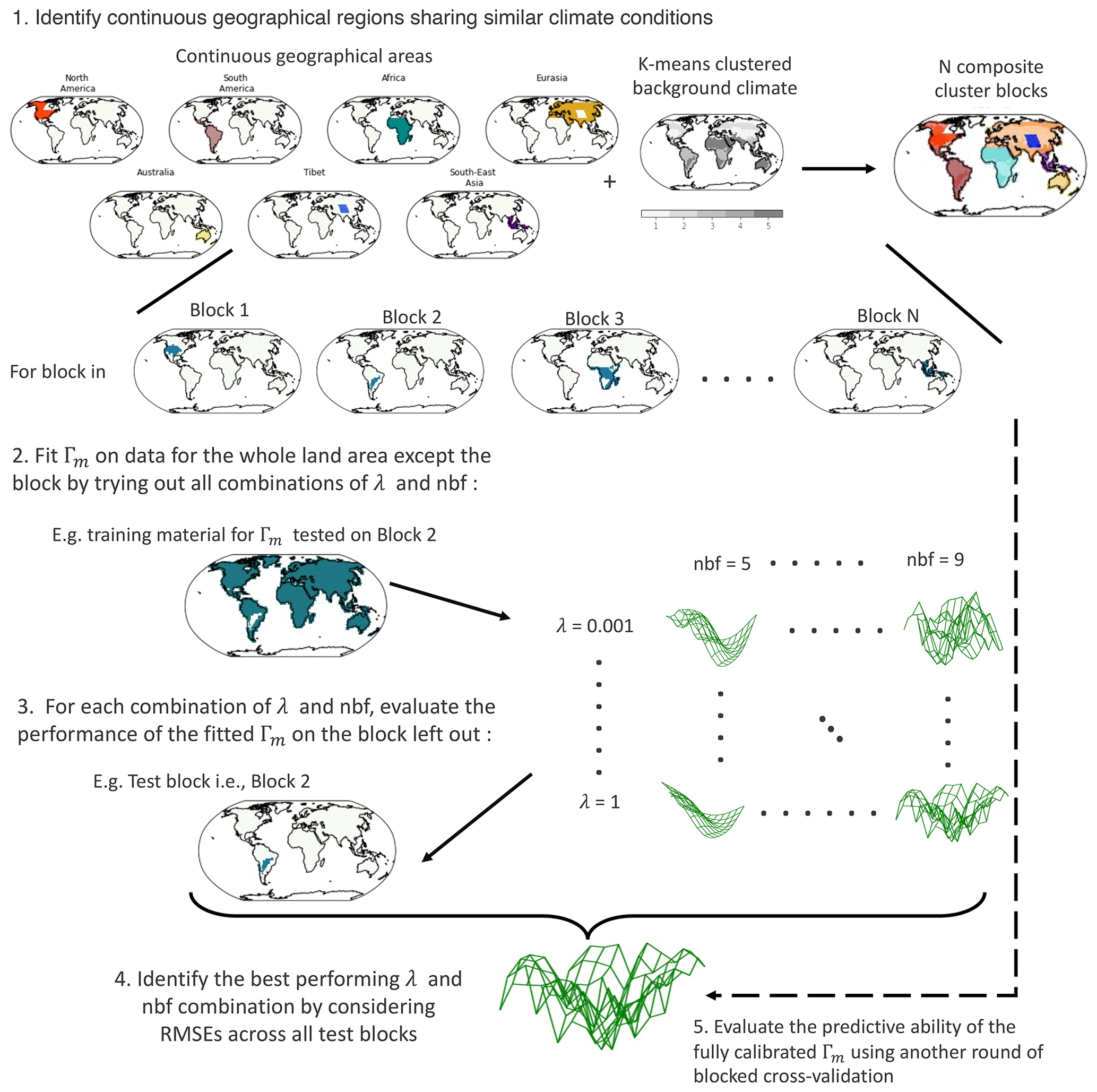
Figure 1Framework of blocked cross-validation used for the calibration and the evaluation of Γm based on its ability to predict the surface temperature response to tree cover changes over climate and continuous geographical regions not considered during model calibration.
3.3 Diagnosing the 2 m air temperature response from changes in surface temperatures
Hooker et al. (2018) were able to derive month-specific relationships between observational night and day surface temperatures () and observational (provided by the Global Historical Climatology Network monthly Menne et al., 2018). They did so by performing both geographical and climate space weighted regression (GWR and CSWR) between observational and observational values so as to obtain grid-point-level coefficients specific to geographical and/or background climate conditions. By taking a stacked generalisation of the GWR and CSWR outputs, Hooker et al. (2018) were able to reconstruct global maps over the period 2003 to 2016 in a geographically and climatically consistent manner.
In this study, we use a model adapted from Hooker et al. (2018) to diagnose from surface temperatures. Ideally, the Hooker et al. (2018) model would be refitted to derive ESM-specific coefficients between ESM surface temperatures and observed data. Given that this study primarily focusses on setting up a conceptual framework, however, we choose to directly apply the original coefficients derived by Hooker et al. (2018) as an initial proof of concept. Before applying the Hooker et al. (2018) model, we first make some modifications to it so as to enable a smooth translation between observed and ESM spaces. In the following subsections, we introduce the modifications made to the Hooker et al. (2018) model and furthermore outline some tests performed to check that the modified version of it applied to ESMs still yields results comparable to those expected from observations.
3.3.1 Modifications of the Hooker et al. (2018) model
values are diagnosed using a modified version of the Hooker et al. (2018) model, which uses values instead of and only considers the GWR coefficient terms,
assuming that the effects of land cover type are minimal on , we then get
where , , and are coefficient terms obtained from GWR. We choose not to use the CSWR coefficient terms as background climates between observations and ESMs are not consistent and there is the additional uncertainty surrounding the evolution of CSWR coefficient terms under changing background climates. Additionally, we use values instead as they are the only available DEF and AFF scenario ESM outputs which are most similar to .
3.3.2 Tests on the modified Hooker et al. (2018) model applied to the ESM space
Since we look at relative changes in , the modifications made to the Hooker et al. (2018) model are expected to have minimal impact as long as the biases in values calculated using ESM values have the same spread as those arising from natural variability within observational values and are thus acceptable. To determine this, we compare the spread of biases obtained when calculating values from observational values to those obtained from ESM outputs for the REF scenario. outputs from the REF scenario are used as we consider them to be representative of the natural variability surrounding values. We approximate the spread of biases by taking into account the natural variability surrounding the surface temperature values and compare them through the following steps:
-
Construct a multivariate Gaussian process across all observational values to generate spatially correlated pairs of which also take into account cross-correlations between and . Generated pairs will act as pseudo-samples that represent the underlying uncertainty due to natural variability within observational data.
-
For each time step of predictions available from the original (Hooker et al., 2018) model (going from 2003 to 2016), perform the following:
-
Generate 100 synthetic pairs of values using the Gaussian process constructed in step 1.
-
Calculate the biases between the prediction available from the original (Hooker et al., 2018) model and those obtained by applying Eq. (2) to the synthetically generated pairs of .
-
-
Take the interquartile range (IQR) of the biases calculated in step (2b) as a measure of their spread.
-
Repeat steps 1–3 for .
-
Check the difference between the IQR calculated in step 3 using ESM values and that calculated using observational values. A positive difference indicates more spread within the biases for -derived values, in which case the biases are not acceptable considering those arising from natural variability within the observational data.
A separate multivariate Gaussian process is constructed for the observational and ESM values in step 1. In order to construct the Gaussian process, we first test the observational and ESM values for normality using a Shapiro–Wilk test (see Figs. D1–D4 in Appendix D). Observational values are normally distributed over all grid points, while ESM values show some grid points (at most 17 % of grid points) where the null hypothesis of being normally distributed is rejected. Given that this is less than half of the grid points, we proceed with applying the multivariate Gaussian process.
3.4 Emulating 2 m air temperature responses to tree cover changes within the SSP scenarios
By predicting the expected surface temperature responses using the calibrated Γm (described in Sect. 3.2.1) and subsequently diagnosing the corresponding 2 m air temperature response using Eq. (3), we can emulate the expected 2 m air temperature response to tree cover changes over the whole land area for any land cover change scenario. In this study, we do so for two Shared Socioeconomic Pathways, SSP2 1-2.6 and SSP3-7.0, for which the underlying narratives and resulting changes in tree cover over the 21st century are presented in Sect. 2.3. We only present the results for changes in tree cover between 2015 and the end of the century (mean changes between 2015 and 2100).
In arriving at the final 2 m air temperature response emulations, we are mindful of the limited training data available for constructing Γm. To account for this, we assess the underlying signal-to-noise ratio in the emulations by considering noise as the parametric uncertainties within Γm conditional on the training sample population. The noise in emulations arising from the parametric uncertainties within Γm is evaluated using a parametric bootstrap procedure (Hastie and Tibshirani, 1986; Wood, 2017). In the following sections, we outline the parametric bootstrap procedure used, followed by how its results allow for evaluation of the signal-to-noise ratio in the final 2 m air temperature response emulations.
3.4.1 Estimating parametric uncertainty in the predicted temperature responses
We quantify the impact of parametric uncertainties within Γm on the ΔTSm,s predictions following a parametric bootstrap method as outlined in Fig. 2 (Wood, 2017; Efron and Tibshirani, 1993). Parametric bootstrapping constitutes first approximating the joint distribution of the coefficients (β) and λ parameter used within Γm, conditional on the training data available, i.e. (step 1, Fig. 2), from which β values are then sampled to estimate surface temperature responses (step 2, Fig. 2). To avoid high computational costs, the joint distribution is approximated by first bootstrap sampling the distribution of λ conditional on the training material, i.e., fλ(λ) (steps 1a–1b, Fig. 2), from which the distribution of β, conditional on both λ and the training material, is constructed over the whole fλ(λ) space (step 1c, Fig. 2), such that . Surface temperature response values are then sampled by drawing β distributions from random parts of the fλ(λ) space (step 2a, Fig. 2) and sampling coefficient values from them (step 2b, Fig. 2), which are then used to estimate ΔTSm,s values (step 2c, Fig. 2).
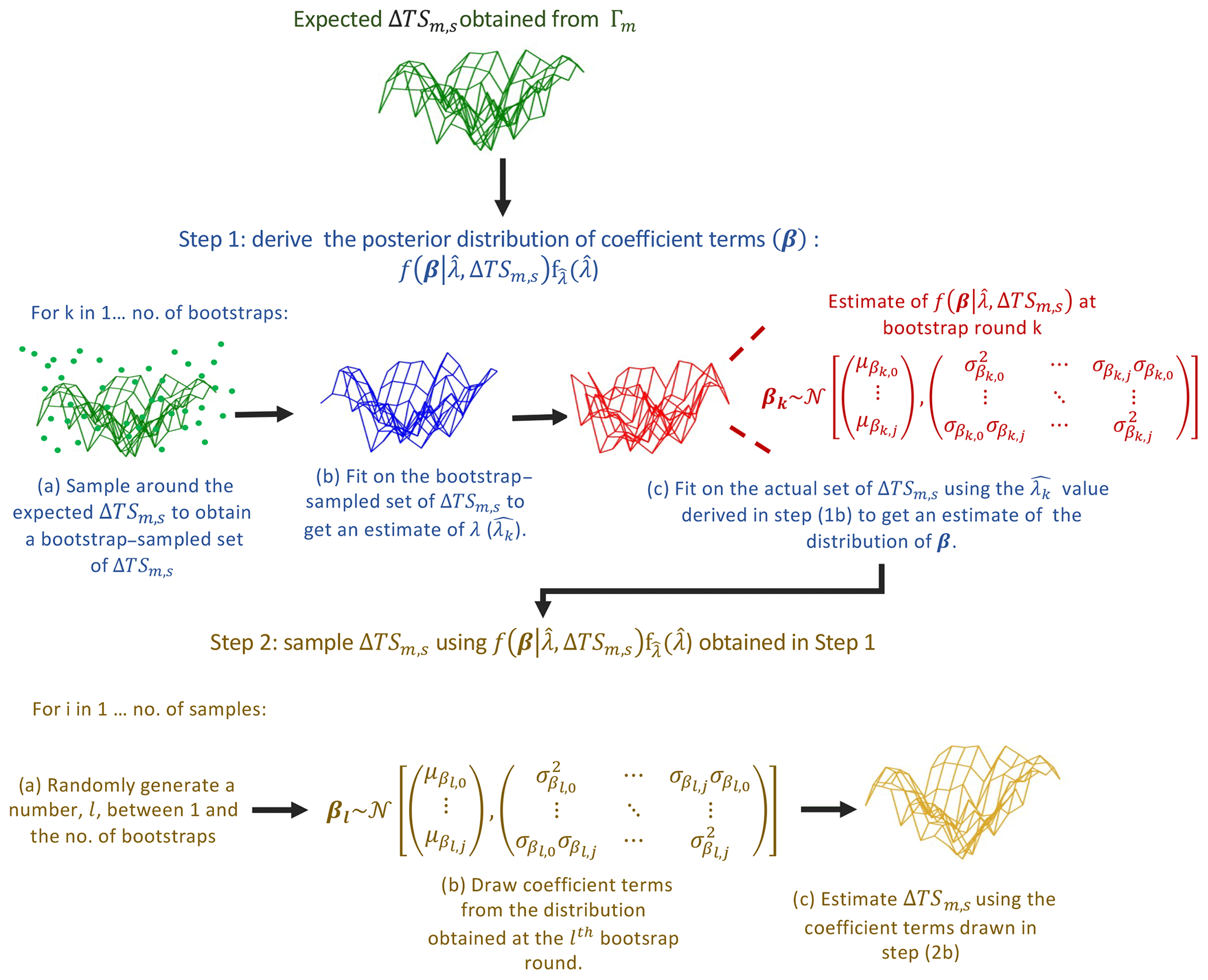
Figure 2Sampling routine of the generalised additive model. First, an approximation of the coefficients' (β) and λ parameter's joint distribution given the available training data is constructed (step 1), from which coefficient terms are sampled to calculate values with step 2. Steps 1a-1b construct the sampling distribution of the λ parameter (fλ(λ)) given the known variability in the training data, and step 1c then constructs the distribution of β conditional on the training data and λ parameter at each point of the fλ(λ) space. As such, the values calculated in step 2 account for the uncertainty in the shape of responses, as modulated by β and λ values.
3.4.2 Evaluating signal-to-noise ratio in the predicted temperature responses
In representing temperature responses under new tree cover change scenarios, we consider the signal-to-noise ratio in the final emulations. Noise constitutes the underlying parametric uncertainty within Γm arising from the training sample population. We start by sampling values from globally for each relevant pixel using the parametric bootstrap procedure outlined in Sect. 3.4.1 and then diagnose for each sample. The β and λ parameter uncertainty spaces are constructed using 10 bootstraps, from which 200 samples are then drawn. We take the mean across all samples as the expected value and the standard deviation across all samples as the underlying parametric uncertainty within the GAM. The signal-to-noise ratio is then obtained as the ratio between the mean and standard deviation values. We consider emulations with a signal-to-noise ratio lower than 0.5 to be insignificant as the underlying parametric uncertainty is double the actual magnitude of the expected response. Given the computational expenses of running ESMs, such gives Γm the benefit of mainly requiring extreme tree cover change scenarios as training material, from which it can further explore all possible outcomes of in-between scenarios itself. It should be noted, however, that this does not remove the benefit of having more training material on top of the extreme scenarios but simply minimises the training data requirements of Γm.
4.1 Blocked-cross-validation results
In this section, we show the calibration and evaluation results of , obtained by performing different sets of blocked cross-validation as described in Sect. 3.2.2 and 3.2.3. The calibration and evaluation results for example months of January and July, which are representative of the hottest and coldest months for the Northern Hemisphere and vice versa for the Southern Hemisphere, are shown. First, we show results from the blocked cross-validation used to calibrate Γm for its optimal λ parameter and number of basis functions (Sect. 4.1.1). Second, we show the results of the blocked cross-validations employed to evaluate the calibrated Γm's performance into no-analogue conditions. No-analogue conditions of background climate (Sect. 4.1.2) and those of tree cover change amounts (Sect. 4.1.3) are considered specifically with a separate blocked cross-validation performed for each. The following subsections show the blocked-cross-validation results for only as this gives a representative idea of the validity of this study's framework. Blocked-cross-validation results for are provided in Appendix C.
4.1.1 Results of model calibration
Figure 3 provides the best-performing λ parameter values and number-of-basis-functions (nbfs) configuration for . Maps of RMSEs calculated between the mean surface temperature response samples drawn by the fully calibrated (200 samples are drawn as described in Sect. 3.4.1), the tree cover changes ΔtreeFrac2015 implemented in the ESM experiments used for training, and the values actually simulated by the ESMs are further provided. The percentage of grid points with RMSE values below 0.5 is indicated above each map. These results are shown for both the DEF and AFF scenarios (only DEF for observations).
The trained on observational data has a λ parameter value of 0.001 for both January and July, which is significantly lower than that of 1 otherwise chosen for all ESMs. This could be because the observationally trained only receives training data for the DEF scenario, which implements large magnitudes of tree cover change localised to specific regions (see Fig. A1 in the Appendix). Thus, lower λ parameter values are favoured to allow for complex representation with higher spatial variability. The observationally trained moreover shows poor performance, with only 34 % of grid points having RMSE values of less than 0.5. This possibly arises from less training being data available for the observationally calibrated (i.e. less grid points as well as only one tree cover change scenario), such that cannot gain as much information to predict with.
All ESMs show higher RMSEs, with a lower proportion of grid points having RMSE values <0.5, for the DEF scenario than the AFF scenario. This could be related to the difficulty in representing the complex response types with high spatial variabilities within the DEF scenario. Such highlights a design consequence of , where tem is fitted smoothly over long, lat, and Δ2015 treeFrac, thus falling short in representing high spatial variabilities as brought about by large magnitudes of localised tree cover change. While CESM2 and EC-EARTH show a varying number of grid points with RMSE values below 0.5 between January and July for the AFF and DEF scenarios, MPI-ESM shows similar performance across both months for the AFF and DEF scenarios. Additionally, MPI-ESM's favours the simplest representation across all ESMs with the lowest number of basis functions chosen for both January and July. Such indicates a smoother response type outputted by MPI-ESM, with deforestation in the tropics not necessarily leading to significant temperature jumps within space.
Overall, mostly displays RMSEs less than or equal to 0.5 for all ESMs. Higher RMSEs (>0.5) are usually localised to regions of extreme magnitudes of deforestation for CESM2 and EC-EARTH. In the case of MPI-ESM, higher RMSEs are localised to different regions depending on the month. For example, in both the AFF and DEF scenarios, MPI-ESM shows higher RMSEs over South America and Australia in January and over southern North America and the Mediterranean region for July. In such, proves itself to be a reasonably flexible framework to represent expected temperature responses to more realistic magnitudes of tree cover change. As noted in the observationally calibrated , a substantial hindrance to 's performance is the availability of training data, where it is recommended to have both directions (i.e. positive and negative) of tree cover changes available for training.
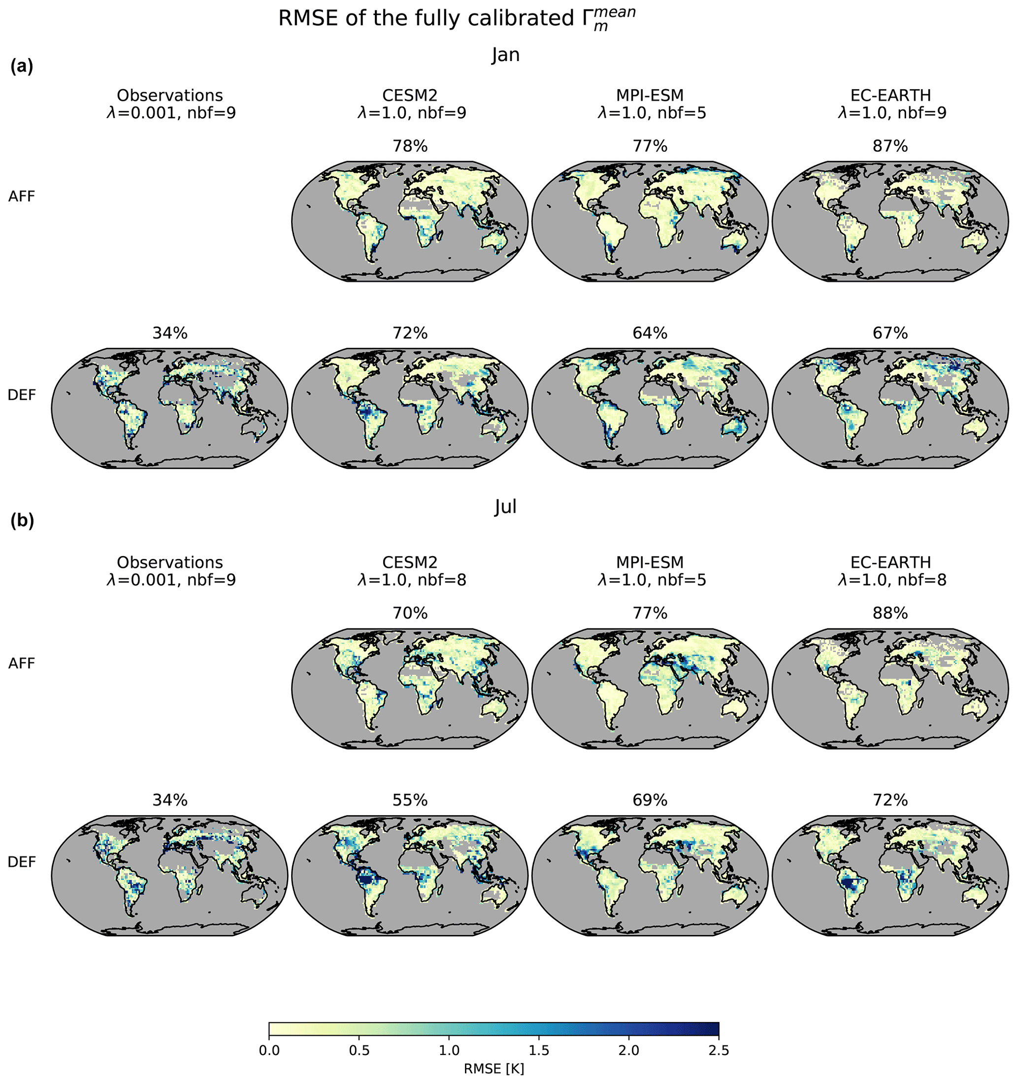
Figure 3Performance of the fully calibrated trained on each full set of observational and ESM data for example months of January (a) and July (b) shown as RMSE maps (rows) for afforestation, AFF (first row), and deforestation, DEF (second row), scenarios. Column headers indicate the training dataset used and the respective λ parameter and number of basis functions (nbfs) chosen during blocked cross-validation. Percentages above each map indicate the proportion of land area with RMSE values of less than 0.5.
4.1.2 Evaluation of under no-analogue background climates
Figure 4 shows RMSEs obtained for 's sampled predictions (200 samples are drawn as in Sect. 3.4.1) in relation to no-analogue background climates aggregated to latitudinal bands for the example months of January and July. Latitudinal bands were chosen to be representative of the different ΔTSm,s response types to tree cover changes (as seen in De Hertog et al. (2022)), namely northern hemispheric, temperate (40 to 65∘ N); subtropical, temperate (10 to 40∘ N); tropical (−15 to 10∘ N); and southern hemispheric (−45 to −15∘ N). Southern-hemispheric results are not differentiated into subtropical and temperate as the sample size of predictions would become too small otherwise. RMSEs are differentiated into those obtained under the AFF scenario and under the DEF scenario, except for observations where RMSEs are only available for the DEF scenario.
For observations and ESMs, the spread in RMSEs displays a month dependency across all latitudinal bands, evidencing the seasonality in responses to tree cover change and also the need for prior background climate information being more important for certain months than others. Despite the spread in RMSEs being large, median values are mostly below 0.5 for ESMs and below 1.5 for observations, which is in line with those seen in Fig. 3, indicating overall good prediction skill for in relation to unseen background climate conditions. Observation RMSEs for DEF at −45 to −15∘ N, however, show significantly higher median values than those in Fig. 3, although this is more likely to be due to data sparsity within the training data for this region, leading to little information being learned by the observationally calibrated for this region.
Across ESMs, DEF in the tropics (−15 to 10∘ N) shows the largest spreads in RMSEs, with slightly higher median values than those of Fig. 3. Given that may underperform within these areas due to the localised, large magnitudes of deforestation (as seen for CESM2 and EC-EARTH in Fig. 3), exploration of its performance into no-analogue tree cover changes is first required before concluding lower prediction skill for unseen background climate conditions within these areas.
4.1.3 Evaluation of under no-analogue tree cover change amounts
Figure 5 shows the median RMSEs (with error bars indicating 50 % confidence intervals) obtained for 's sampled predictions in relation to no-analogue tree cover changes aggregated to latitudinal bands for the example months of January and July. For observations and ESMs, magnitudes and patterns of RMSEs are similar between January and July across all latitudinal bands, contrary to what has been found for the predictive ability in no-analogue background climate conditions Sect. 4.1.2. This is expected as the way that local temperature response to tree cover changes depends on the season varies across background climates (and mainly across the latitudes; see, for example, Li et al., 2015) and is thus intuitively more important for representing seasonality in values.
Median RMSEs for in the tropics are higher than those seen for DEF in Fig. 4, indicating that the prediction skill for in the tropics is more dependent on the availability of training information for similar tree cover changes than for similar background climate. MPI-ESM is an exception to this, displaying much larger RMSEs for DEF in Fig. 4. Such could result from MPI-ESM outputting a weaker response to tree cover change in the tropics, as previously suggested in Sect. 4.1.1, making the availability of prior background climate information the main factor influencing 's prediction skill.
Observations, CESM2, and EC-EARTH show an increase in RMSEs across all latitudinal bands as Δ2015 treeFrac values move towards the more extreme ends (−1 for observations and ±1 for CESM2 and EC-EARTH), sometimes even reaching RMSEs higher than those seen in Fig. 3. This indicates lower prediction skill for in relation to unseen, extreme tree cover change conditions for observations, CESM2, and EC-EARTH. Nevertheless, the resolved skill seen in Fig. 3 verifies the need to have a training dataset representative of the extreme ends of tree cover change, as responses may systematically become more non-linear with increasing magnitudes of tree cover change.
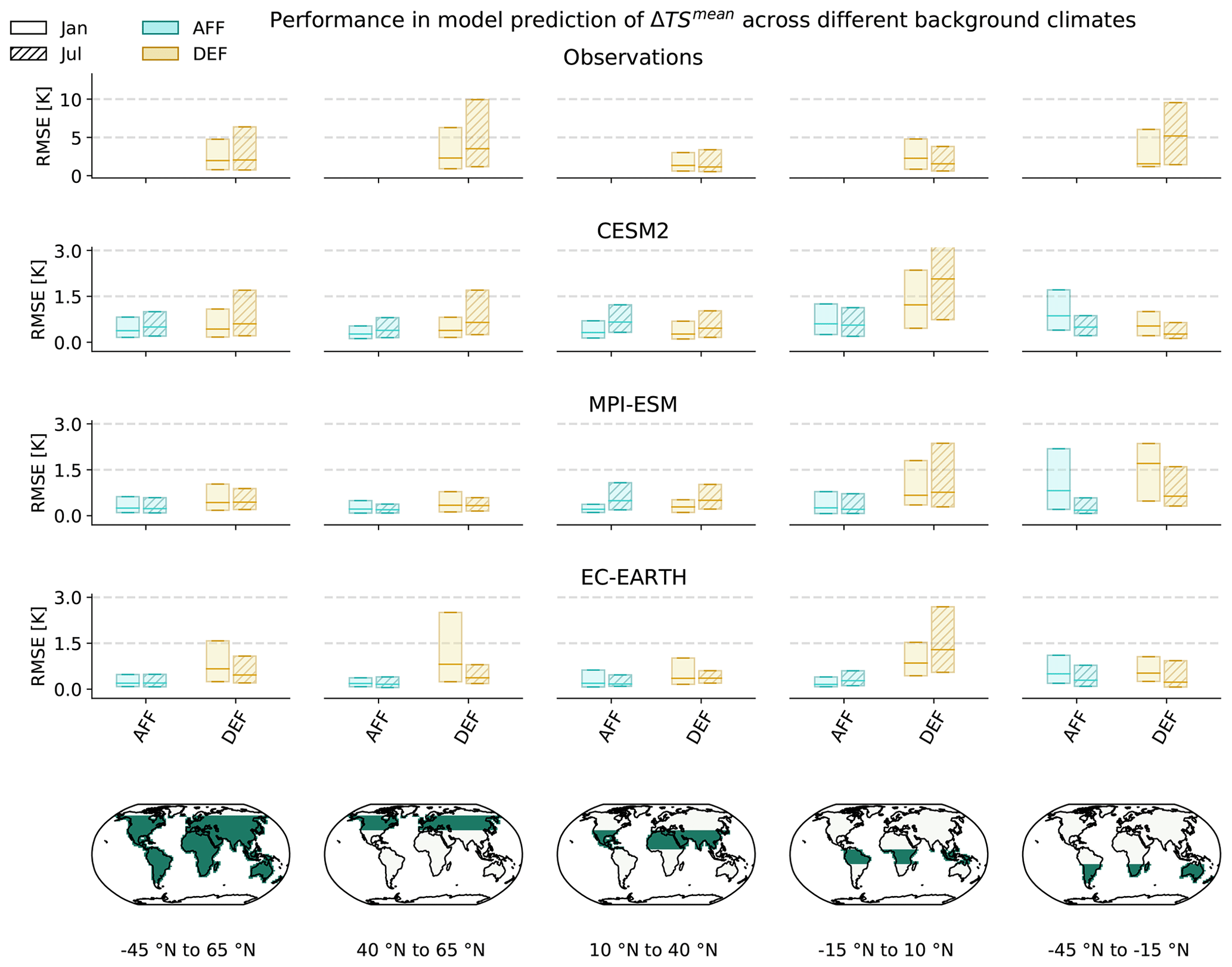
Figure 4Evaluation of 's predictive ability under non-analogue background climate conditions. Test set RMSEs obtained during blocked cross-validation with blocks clustered according to background climate and continuous geographical region (as shown in Fig. B1 in the Appendix) are considered. RMSEs are shown for the months of January (unhatched) and July (hatched) and are aggregated to latitudinal band (columns) and direction of tree cover change, with yellow indicating a negative change (DEF) and blue indicating a positive change (AFF). The box plots indicate the median RMSEs, as well as the associated interquartile ranges. Note that the scale used for observations (upper row) is different.
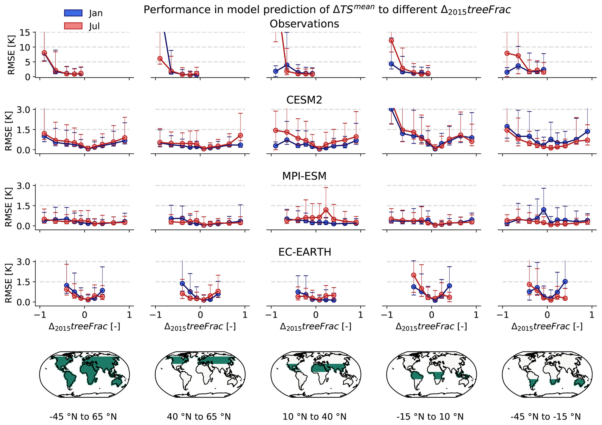
Figure 5Evaluation of 's ability to predict across Δ2015 treeFrac. Test set RMSEs were obtained during blocked cross-validation using blocks identified by gathering grid cells that underwent similar Δ2015 treeFrac (grouped according to sign of change and absolute value, as binned into [0.01,0.15), [0.15–0.3), [0.3–0.5), [0.5–0.8), and [0.8–1.0]) within continuous geographical regions. RMSEs are shown for January (blue) and July (red), are aggregated to latitudinal bands (results for each band are shown in a different column), and are plotted against the centre of each Δ2015 treeFrac bin. The dots indicate the median RMSEs, while the error bars indicate the associated interquartile range. Note that the scale used for observations (upper row) is different.
4.2 Illustration of outputs
In this section, we showcase the results of when predicting for any amount of tree cover change compared to 2015 levels and across the world. A select tree cover change value is applied to all grid points, and is then used to predict the temperature responses for that tree cover change. Figure 6 illustrates the mean predictions as well as their 95 % interval calculated across all grid points within a given latitudinal band. We choose the same latitudinal bands used in Figs. 4 and 5 .
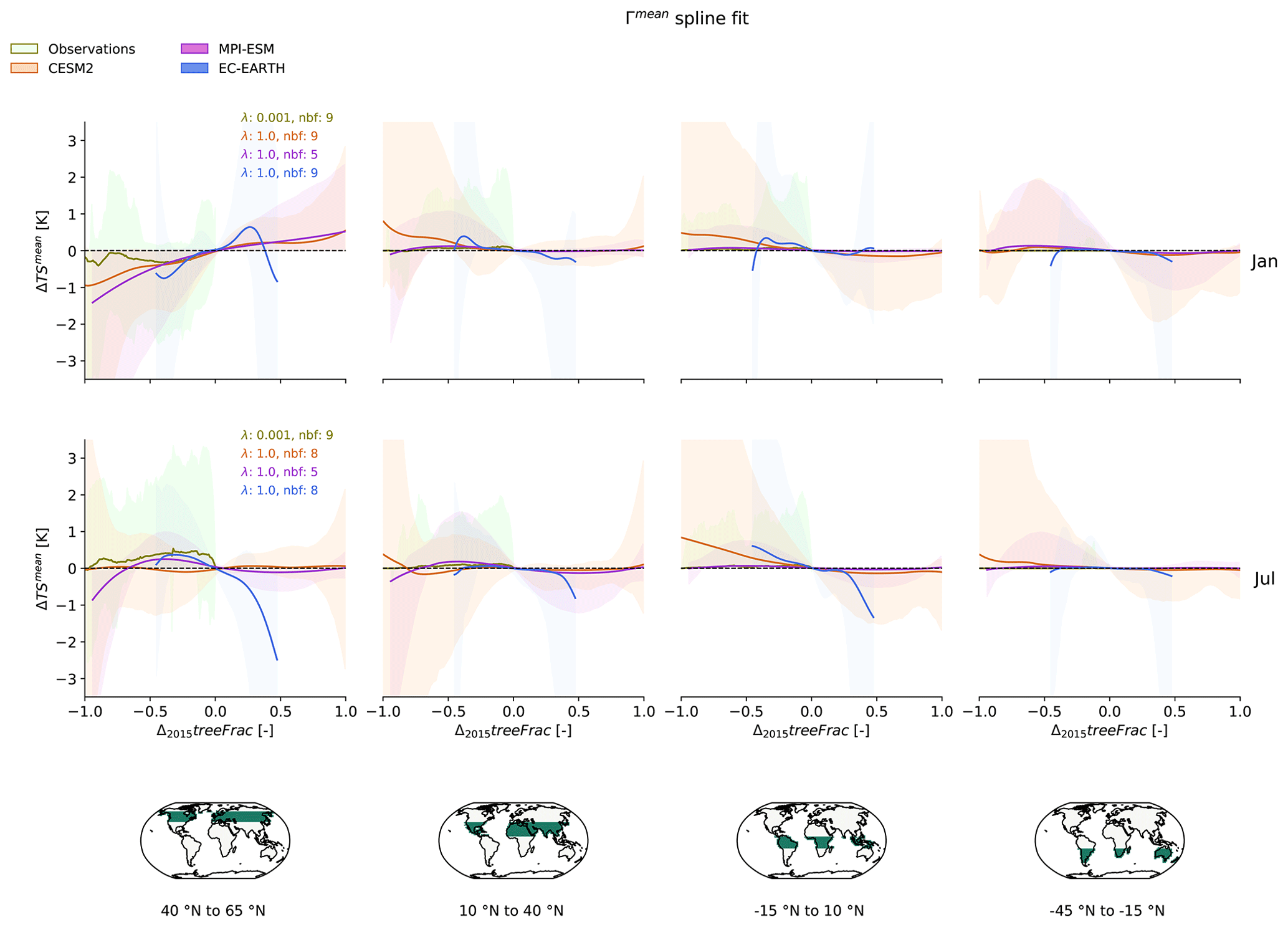
Figure 6's depiction of , shown for observations and ESMs (colours) for the months of January (first row) and July (second row) across the whole range of Δ2015 treeFrac and aggregated to latitudinal bands (columns). λ parameters and number of basis functions (nbfs) chosen through blocked cross-validation are given in the first column of their respective month and are colour coded according to their respective training data (observations or ESMs). Solid lines represent the mean predictions, and the surrounding band represents the 95 % interval calculated over predictions for all grid points within the respective latitudinal band.
As a preliminary check, the predictions can be roughly compared to the ESM outputs for the idealised AFF and DEF simulations as analysed by De Hertog et al. (2022). Only a rough comparison is possible, however, as we generate predictions for tree cover change maps of constant values across grid points, whereas the tree cover change maps applied within the AFF and DEF scenarios vary in values across grid points since they represent the full expansion of forest and/or cropland relative to the 2015 period. To this extent, predictions shown in Fig. 6 correspond well in terms of direction and magnitude to the results shown in Duveiller et al. (2018c) (for observations) or in De Hertog et al. (2022) (for ESMs; compare with their Figs. 2, 3, 5, and 6). For example, over the northern-hemispheric temperate region (40 to 65∘ N) in January, indicates a cooling (warming) following deforestation (afforestation) when trained on all ESMs and observations, while the temperature response in July is less clear but still rather indicates a warming from deforestation over these regions. Moreover, is notably able to capture the inter-ESM spread in values. For example, in the latitudinal band of 40 to 65∘ N, EC-EARTH-based predictions show a cooling trend after +25 % tree cover change in contrast to the warming trend seen in other ESMs. Such a difference was also noted in De Hertog et al. (2022) and was attributed to the lower amounts of boreal afforestation implemented.
Over all latitudinal bands and months shown, the largest 95 % intervals occur towards the extreme ends of tree cover change for both observations and ESM-based predictions. This is especially the case for deforestation, where the 95 % intervals are generally larger than those of afforestation. Higher 95 % intervals at extreme ends of tree cover change result from fewer grid points which undergo more extreme tree cover changes, ergo less training material. This highlights once more the higher uncertainty in the predictions by for extreme amounts of tree cover change (in both directions).
Mean observation-based predictions remain close to 0 across all latitudinal bands for both January and July owing to the high data sparsity which makes it difficult to extract significant responses during training. Nonetheless, observation-based 95 % intervals are in general agreement with those of ESMs across all latitudinal bands and months shown.
4.3 Surface to 2 m air temperature diagnosis
In this section, we apply the modified (Hooker et al., 2018) model (Eq. 3) to the outputs of and so as to derive the expected responses to tree cover change. Results are only shown for CESM2 as tree cover changes implemented in the experiments run by this ESM cover the whole range of possible Δ2015treeFrac (unlike observations and EC-EARTH) and provide local values (not available from MPI-ESM otherwise). We first ascertain that applying Eq. (3) in the ESM space does not introduce additional biases to predictions on top of those arising from the natural variability in observed values, after which we proceed with predicting responses based off outputs.
4.3.1 Tests on the modified Hooker et al. (2018) model applied to the ESM space
Figure 7 compares the spread of biases in calculated using ESM values to that obtained when using observational values. Positive values indicate more spread within the biases of ESM-derived values, suggesting that biases outside the range of those arising from natural variability may occur when calculating .
Across most months, fewer than 40 % of grid points have positive values, and these mostly occur in the Northern Hemisphere for the months between and including January and June. Such may result from the change in the length of day during these months such that values do not necessarily correspond to the values. To be specific, the times of overpass for measuring and are fixed at 01:30 and 13:30 LT (local time at the Equator), respectively; however, given the longer nights in northern-hemispheric winters, is likely to occur later and earlier than these times.
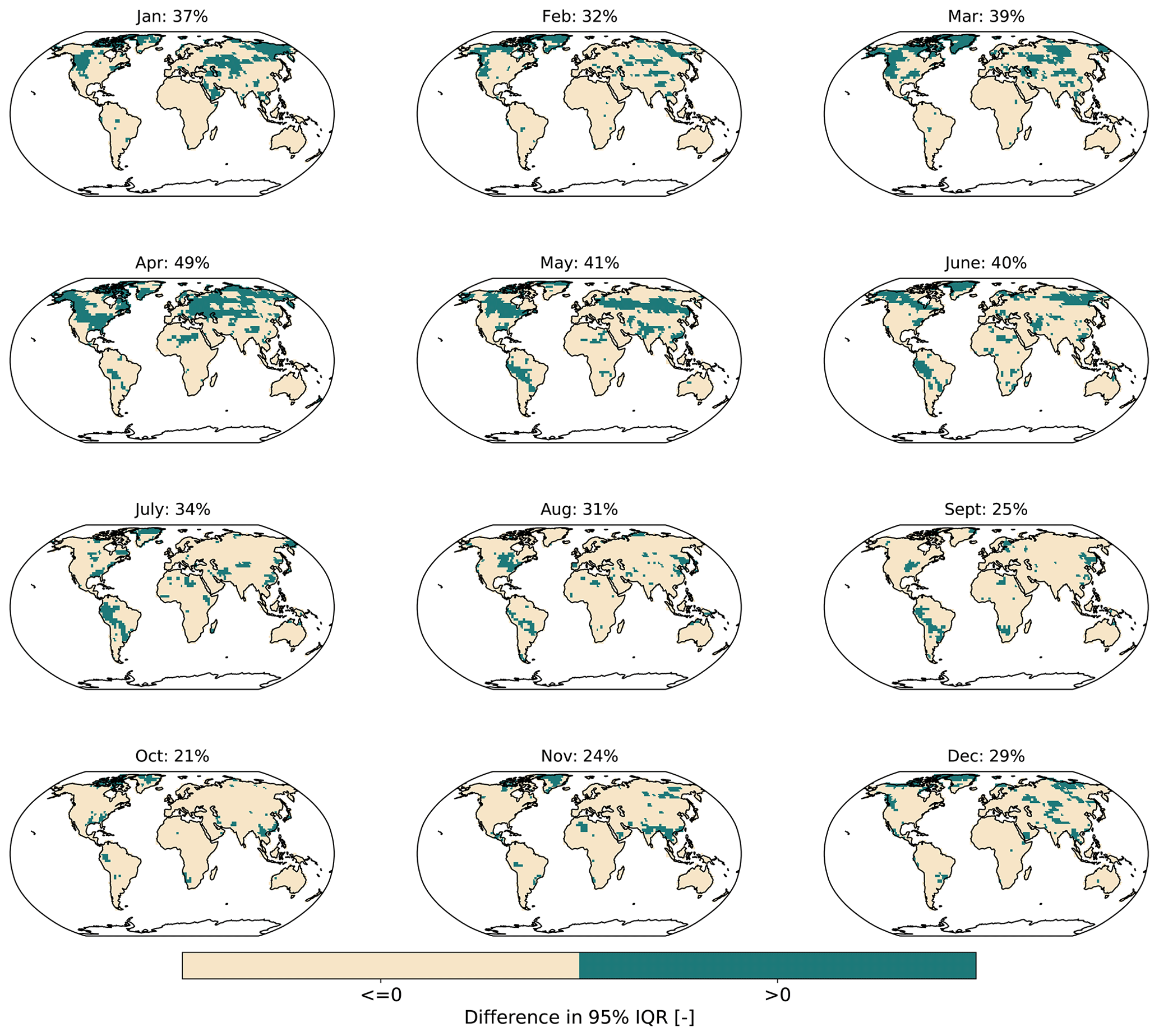
Figure 7Differences between the spread of biases for ESM vs. observationally derived values, obtained as described in Sect. 3.3. The inter-quartile range (IQR) is considered as a measure of spread, and results are shown for CESM2 across all months. Percentage values indicate the proportion of land grid points where ESM-derived values have a larger spread in bias as compared to observationally derived values.
4.3.2 2 m air temperature diagnoses
Since fewer than half of the grid points have positive values and since such values are isolated to certain months and geographical areas, we proceed with diagnosing from values outputted by . The calibration and evaluation results for are available in Appendix C and show similar results as those seen in Sect. 4.1, namely minimal additional RMSEs when predicting in relation to no-analogue conditions sampled out of the training dataset as compared to when predicting after having seen the full training dataset (i.e. comparing RMSE values from Figs. C3 and C4 in the Appendix to those of Fig. C2 in the Appendix). It should be noted that predictions show high RMSEs, especially for the DEF scenario where fewer than half of the grid points have RMSEs lower than 0.5. In relation to the absolute values (see Fig. C1 in the Appendix), however, these RMSEs are of similar relative magnitude to those of and . Moreover, RMSEs of are of similar magnitude when predicting in relation to no-analogue conditions as when predicting after having seen the whole training dataset.
Figure 8 shows the values obtained at different tree cover change values alongside the and predictions for the example months of January and July. Patterns of and predictions correspond well to one another and generally correspond well to values as derived in another study using the same ESM (Meier et al., 2018). An exception here is northern-hemispheric July values, for which a cooling was observed in Meier et al. (2018) in contrast to the warming seen in the training material used within this study (see Appendix C, Fig. C1). Such a discrepancy could arise from too-large albedo responses shown by CESM2 and highlights the caveats of diagnosing from , where physical inconsistencies in the surface temperature responses as represented within ESMs can be transferred to during diagnosis. Nevertheless, the task of Γm is to mimic ESM outputs irrespective of their realism, and to this end, the statistically derived relationships for in relation to tree cover changes match those of the ESM outputs trained on.
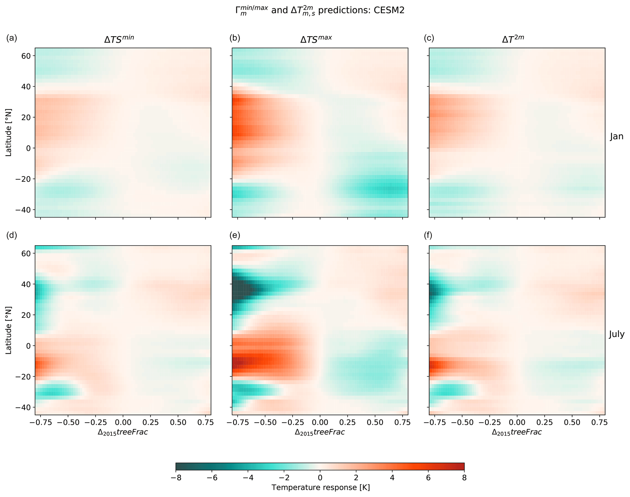
Figure 8Latitudinally aggregated given by (a, d, b, e) shown for CESM2 for the months of January (a, b, c) and July (d, e, f) across the full range of Δ2015treeFrac. The resulting values obtained using the modified (Hooker et al., 2018) model are shown in the third column.
4.4 Exploration of tree cover change effects within SSP scenarios
In this section, we showcase the results of applying TIMBER v0.1 calibrated on simulations conducted with CESM2 to the scenarios of future tree cover changes in SSP1-2.6 and SSP3-7.0. We employ the sampling method as described in Sect. 3.4 such that parametric uncertainties within the GAM are also represented. This provides a first step towards statistically emulating responses to tree cover change in a manner that not only provides the expected response but also gives an idea of the signal-to-noise ratio within predictions.
Figure 9 shows maps of end-of-century tree cover changes (shown in the first column) under SSP 1-2.6 and SSP 3-7.0 and their associated mean responses (second column), obtained by sampling values from , applying Eq. (3) to get and taking its sample average. The signal-to-noise ratio is furthermore given by taking the ratio between the absolute mean value and its standard deviation calculated across sample results for (third column). We consider areas with a signal-to-noise ratio lower than 0.5 to have an insignificant temperature response as their surrounding parametric uncertainty is double that of the magnitude of response.
SSP 1-2.6 shows substantial cooling from afforestation in southern Africa and Brazil for both January and July. A substantial July warming due to deforestation can also be seen in the Tibetan Plateau due to deforestation. SSP 3-7.0 shows a significant January and July warming due to deforestation in Central Africa, the Tibetan Plateau, and South America. Western North America shows a significant cooling from deforestation, especially in July, while parts of East Asia show significant cooling from afforestation for both January and July.
In general, areas with a tree cover change lower than 0.1 in magnitude tend to have a signal-to-noise ratio lower than 0.5 and thus an insignificant temperature response. Such systematically lower signal-to-noise ratios indicate that Γm is not only aware of the lack of information it has for smaller changes in tree cover but can also infer that temperature responses to such tree cover changes are likely to be trivial.
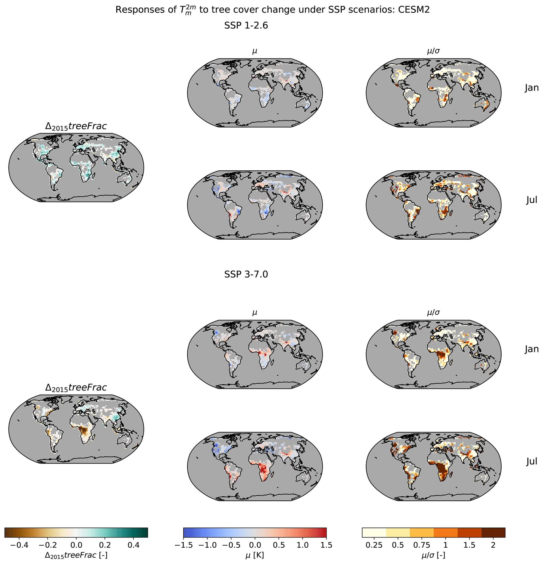
Figure 9 values resulting from end-of-century changes (i.e. 2100) relative to 2015 in tree cover for SSP 1-2.6 (upper panel) and SSP 3-7.0 (lower panel) scenarios for the months of January (top rows) and July (bottom rows). Mean values (second column) and their signal-to-noise ratios (third column) calculated over the sampling distributions are shown. Δ2015 treeFrac maps are given in the first column, and grid points with are not considered.
This study presents TIMBER v0.1, a conceptual framework for representing monthly temperature responses to changes in tree cover. TIMBER v0.1 starts by modelling minimum, mean, and maximum surface temperature responses to tree cover change with a month-specific GAM, which is trained over the whole globe; 2 m air temperature responses are then diagnosed from the modelled minimum and maximum surface temperatures using observational relationships derived by Hooker et al. (2018). Such an approach maintains the ESM-specific temperature response to tree cover change whilst ensuring a constant diagnosis and observationally consistent definition of 2 m air temperature.
The GAM is evaluated for its ability to predict in relation to unseen, i.e. no-analogue, background climate and tree cover change conditions. This is done using a blocked-cross-validation procedure in order to account for the spatial structure of the data when splitting into subsamples used for training and testing. Overall, the GAM shows good skill in predicting in relation to no-analogue conditions, with minimal RMSEs in addition to those that occur when predicting after having seen the full training dataset and thus all available background climate and tree cover change information. Such provides confidence in the GAM's ability to derive meaningful relationships from the training data provided by the ESMs. Nevertheless, poorer representation for extreme, localised tree cover changes was identified, such as for deforestation in the tropics, most likely due to the difficulty in adequately representing high spatial variability.
When predicting in relation to new tree cover change scenarios, we are especially mindful of the training data only including grid points which experience extreme tree cover change in the training simulations. To this extent, surface temperature responses are sampled from the GAM in a manner that explores all possible shapes of responses in between the two extreme ends of tree cover change as provided by the training data; 2 m air temperature responses are then diagnosed from the sampled surface temperature responses, and relevant responses are identified as those that have a high signal-to-noise ratio (>0.5).
The final outputs of TIMBER v0.1 are demonstrated for SSP 1-2.6 and SSP 3-7.0. Generally, areas with less than ±10 % tree cover change render a low signal-to-noise ratio, which is intuitive as responses to such low changes in tree cover are likely to be minimal. Employing TIMBER v0.1 thus provides an avenue to explore the impacts of tree cover change and their underlying uncertainty due to the availability of training data and model calibration. It should be stressed that, given the lack of comparable ESM simulations that employ the checkerboard approach to isolate local signals of land cover changes, TIMBER's outputs cannot be thoroughly validated and must therefore be cautioned with the limitations of its current set-up, specifically that they are produced with limited amounts of training data and that the 2 m air temperature is diagnosed using observational relationships – as provided by Hooker et al. (2018) – directly applied to the ESM space. In the following subsections, we further highlight areas of potential improvement, elaborate upon the suitable modes of application for TIMBER v0.1, and detail possible further developments.
5.1 Areas of potential improvement
One area of potential improvement pertains to the model calibration procedure. When inspecting the calibrated λ parameter values and the number of basis functions, the limits of values cross-validated for (0.001 and 1 for the λ parameter and 5 and 9 for the number of basis functions) seem to be favoured. Reasons behind this could be (1) the blocked cross-validation sometimes removes too-large chunks of data, leading to an overestimation of RMSEs chosen; and/or (2) the range of λ parameters and/or number of basis function values calibrated for is too narrow. The first reason could be tackled by further splitting the blocks such that each block has a predefined number of samples. Alternatively, the GAM could be fitted over specific climate regions, and blocked cross-validation could be conducted with uniformly sized blocks composed along latitude and longitude dimensions, although, here, it is likely that the complete spectrum of tree cover change information will be lost for some regions. The second reason is easily solved by cross-validating over a larger range of values.
Another area of improvement could be to derive ESM-specific coefficients for the Hooker et al. (2018) model. Such would entail fitting for the relationships between ESM minimum and maximum surface temperatures and the observational 2 m air temperatures as used by Hooker et al. (2018). Since the additional biases introduced by using the original Hooker et al. (2018) coefficients on the ESM surface temperatures were ascertained to be minimal (Sect. 4.3.1), such an exercise would mostly target deriving the complete Hooker et al. (2018) model for each ESM. The resultant ESM-specific Hooker et al. (2018) models obtained would allow for more consistent 2 m air temperature diagnoses, facilitating better comparison. Furthermore, considering that the difference between night and day surface temperatures (that are used as predictors in the original Hooker et al. (2018) model) and minimum and maximum surface temperatures may also be quite large (e.g. minimum winter temperatures in the Northern Hemisphere are likely to occur after the time of overpass when nighttime temperatures are measured), such would be an essential step in being able to accurately diagnose 2 m air temperatures.
5.2 Modes of application
TIMBER v0.1 provides a framework to explore local-level temperature implications of tree cover changes in an agile manner under different tree cover change scenarios. TIMBER v0.1 can be used as both a standalone device and as a supplement to other emulators. It should be noted that, to provide complete representation of the biophysical effects of tree cover change, albedo and thermal fluxes would have to be considered as well. To this extent, the temperature responses provided by TIMBER arise from a combination of the effects of albedo and thermal flux responses to tree cover changes on the atmospheric energy balance. Here, we summarise some key takeaways pertaining to the use of TIMBER v0.1 for generating new tree cover change scenarios.
Upon inspection of the response patterns across all tree cover changes (Fig. 6), inter-ESM differences become quite apparent. Such differences are continuously studied and mainly arise from differences in model physical representation (Boisier et al., 2012; Lawrence et al., 2016; Lejeune et al., 2018; Davin et al., 2020; Boysen et al., 2020; De Hertog et al., 2022). Being able to train the GAM across all ESMs presents the opportunity to capture these uncertainties due to model physical representation, which may sometimes be higher than the parametric uncertainty within the GAM given the training data. When exploring new tree cover change scenarios, the need to have as many ESMs represented should therefore be emphasised. Moreover, the outputs of TIMBER v0.1 should always be interpreted as representative of the ESM-simulated world, which does not necessarily translate to observed reality.
In applying TIMBER v0.1 to different tree cover change and climate scenarios, it should furthermore be acknowledged that the effects of initial starting conditions and those of background global warming levels have not been accounted for (e.g. see Winckler et al., 2017b, for the possible effects of initial starting conditions on temperature responses to land cover changes). In order to represent such effects, TIMBER would require more training data. Furthermore, if the Hooker et al. (2018) coefficients are recalibrated for the ESM space, the impacts of changing climate on 2 m air temperatures could well be represented through the CSWR coefficients. Nonetheless, outputs of TIMBER v0.1 should more so be treated as hypothetical sensitivities and not definite responses.
Finally, as a conceptual framework, TIMBER v0.1 comes with its limitations that need to be accounted for and improved in future versions. A noteworthy limitation is the diagnosis of 2 m air temperature that relies on the modified Hooker et al. (2018) model. Such a set-up was implemented so as to enable constant diagnosis and definition of 2 m air temperatures across ESMs and observations. However, since the original Hooker et al. (2018) model takes night and day surface temperatures as predictors, whereas the modified model used in this study takes minimum and maximum surface temperatures, current 2 m air temperature predictions should be treated with caution. As seen in Fig. 7, such differences are expected to introduce minimal biases since TIMBER looks at relative changes and not absolute values. However, for select months and regions (e.g. winter in Europe and North America), there are still added biases as night and day surface temperatures do not necessarily correspond to minimum and maximum surface temperatures. An additional limitation to TIMBER is the lack of available ESM data to evaluate it against. Such a problem was circumvented in this study by synthesising the closest representation to no-analogue condition predictions for TIMBER. Nevertheless, when applying TIMBER to different scenarios, predictions should always be treated as approximations. To this extent, the signal-to-noise ratio calculation from TIMBER is an essential feature as it represents the model confidence in predictions based on the available training material.
5.3 Future developments
It would be possible to extend TIMBER v0.1 to represent other impact-relevant climate variables. A variable to start with could be relative humidity, from which metrics such as wet-bulb globe temperature (WBGT) and labour productivity could be derived. In doing so, variable cross-correlations between temperature and relative humidity should be conserved, such that compound events – which largely affect WBGTs – are sufficiently captured. To this extent, a vectorised generalised additive model (VGAM) (Yee and Stephenson, 2007) could be employed, which retains variable cross-correlations by constructing a multivariate conditional probability distribution e.g. by using a bi-normal distribution as opposed to the normal distribution used within this study.
In its current set-up, TIMBER does not differentiate between plant functional types (PFTs). Temperature responses to tree cover changes, however, may differ between different PFTs. For example, needleleaf trees in temperate regions are associated with a stronger winter warming as compared to broadleaf trees, which otherwise lose their foliage during winter (Duveiller et al., 2018b). Representing the temperature responses to different PFTs instead of treating tree cover fraction as a single element would thus further enrich the outputs of TIMBER. A starting point to this could be differentiating between needle- and broadleaf trees. Each of these tree types could be treated as separate tensor spline terms within the GAM, and the final temperature results would be obtained by adding both terms. When doing so, the potential model accuracy gained should be assessed in relation to the added model complexity (i.e. increase in the number of tensor spline terms). Given that needle- and broadleaf trees are unevenly spread geographically (where broadleaf trees occur more in the tropics and needleleaf trees occur more in the temperate regions), it may also be worth training a separate GAM per geographical region so as to get an even representation of needle- vs. broadleaf trees, as well as to prevent model overfitting.
Looking into other land management practices such as irrigation and wood harvest could also be of interest, particularly as their effects on surface temperatures are expected to be similar in magnitude compared to those due to land cover changes (Luyssaert et al., 2014). In doing so, customisation of TIMBER v0.1's framework in relation to the land management practice of choice could be necessary. For example, when looking at irrigation, the implementation of irrigation can be extremely localised and seasonal (Thiery et al., 2017, 2020), and it would be preferable to train the GAM as region specific and across all months instead of month specific and across all grid points. To this extent, the GAM has the advantage of not prescribing any functional form, giving it flexibility in deriving climate responses to different types of LCLM forcings regardless of the format of the training data. In order to jointly explore future tree cover and GHG scenarios, coupling TIMBER v0.1 with other temperature emulators such as MESMER-M or -X (Beusch et al., 2020; Nath et al., 2022b; Quilcaille et al., 2022) also proves to be worthwhile. In doing so, care would have to be taken to not double-count the tree cover change signal as MESMER-M and -X are trained on SSP runs, which contain both GHG and tree cover change signals. Accordingly, it is advisable to first model the expected tree cover change signals within the SSP runs using TIMBER v0.1, following which MESMER-M or -X can be trained on the SSP runs with the modelled tree cover change signals removed.
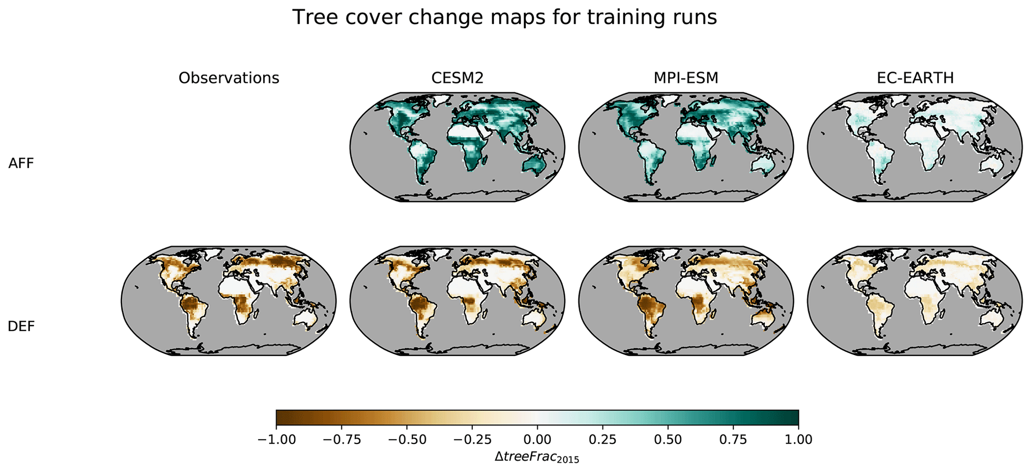
Figure A1The leftmost column shows tree cover change maps for full deforestation relative to the year 2015, as derived by Duveiller et al. (2018c) using observational data. The second to fourth columns show tree cover change maps relative to the year 2015 implemented in the LAMACLIMA afforestation, AFF (top row), and deforestation, DEF (bottom row), experiments in the CESM2, MPI-ESM, and EC-EARTH ESMs.
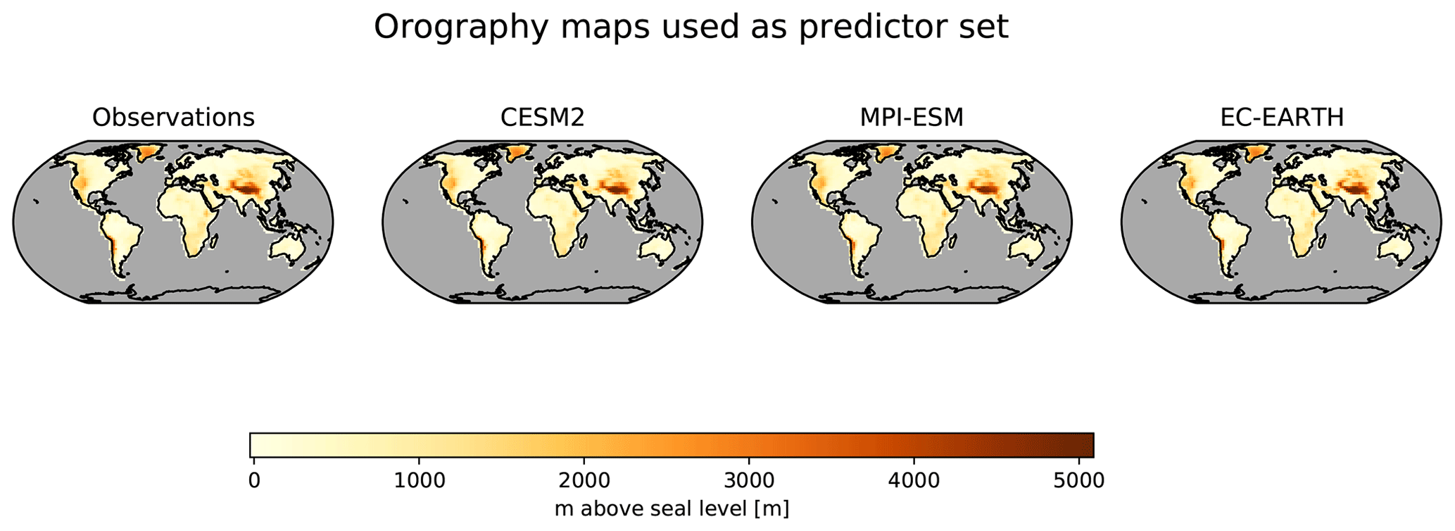
Figure A2Orography features, defined as metres above sea level, used in input predictor matrix for Γm for observations and ESMs (columns).
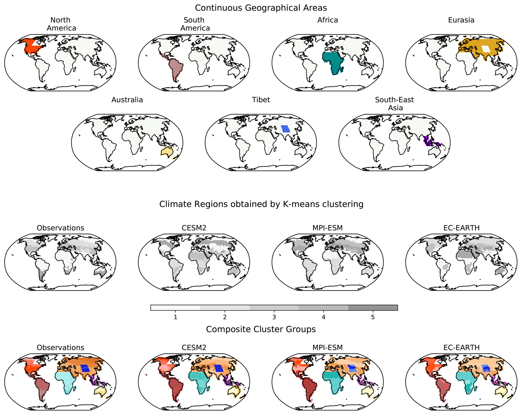
Figure B1Composite cluster blocks obtained by combining clusters of grid points with similar background climate and continuous geographical area. Grid points are clustered into groups with similar background climate using K-means clustering with temperature and relative humidity as indicator variables.
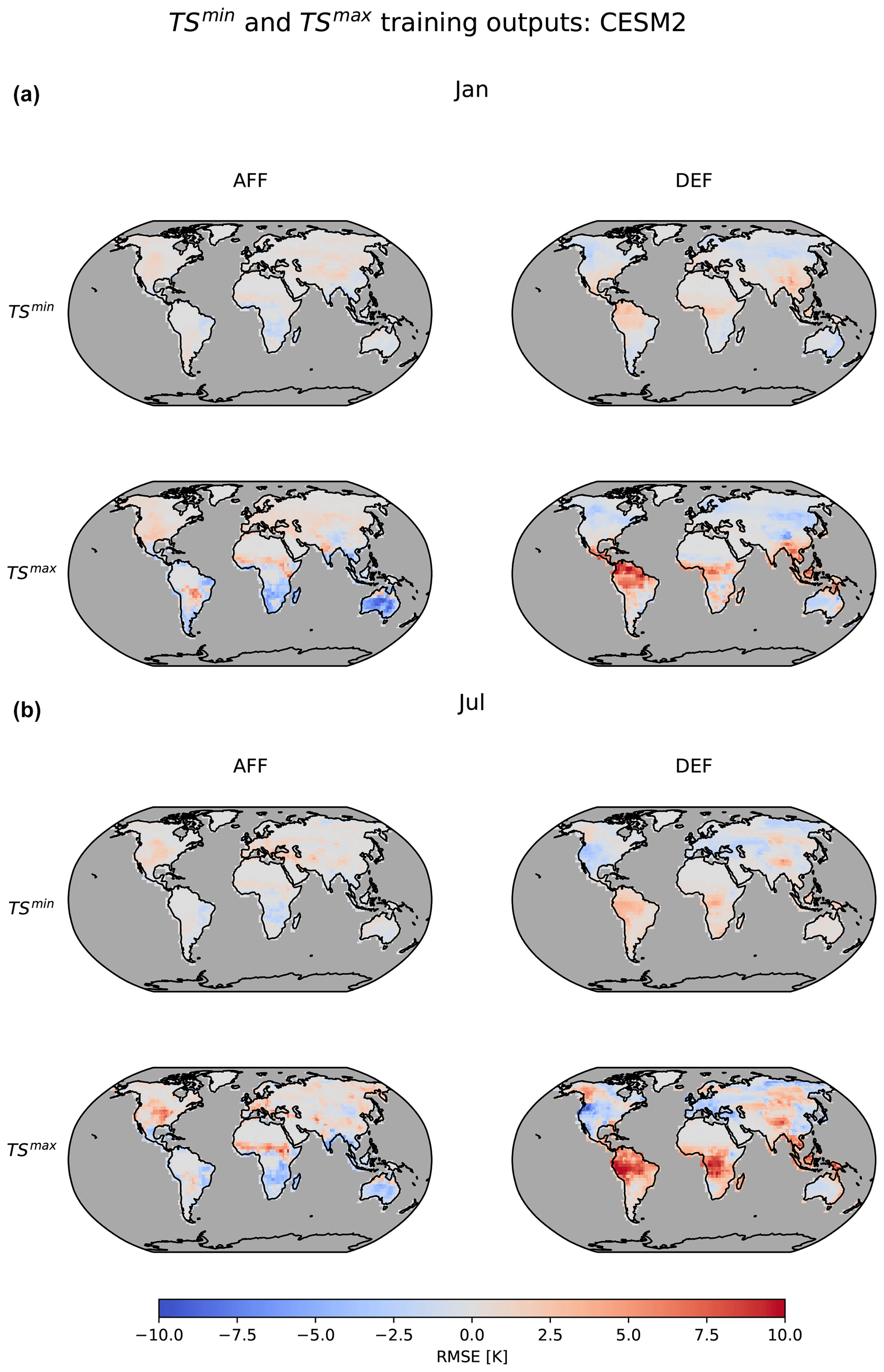
Figure C1 responses (rows) from the LAMACLIMA afforestation, AFF, and deforestation, DEF, experiments (columns) for the months of January (a) and July (b).
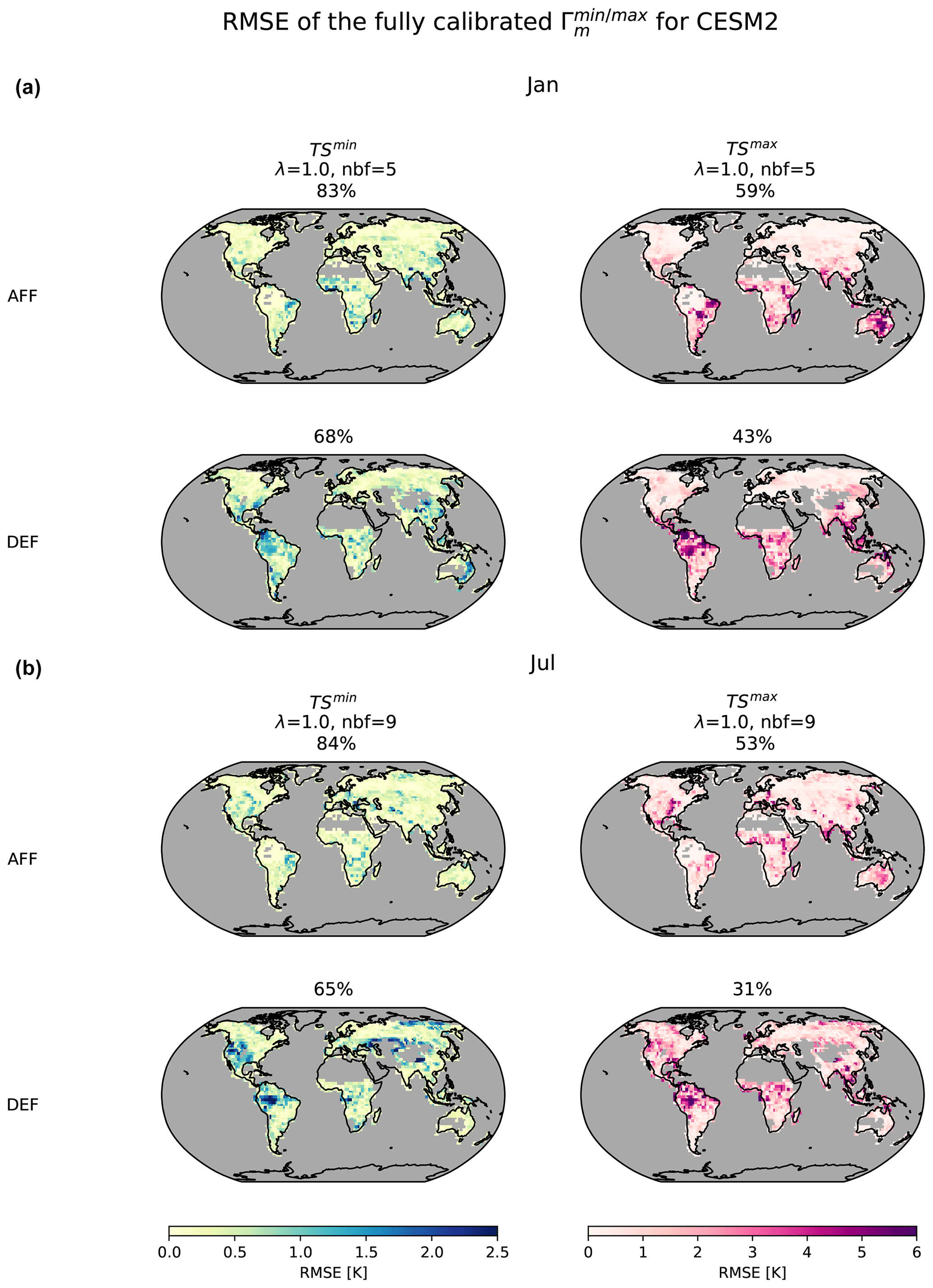
Figure C2Same as Fig. 3 but for CESM2, TSmin, and TSmax.
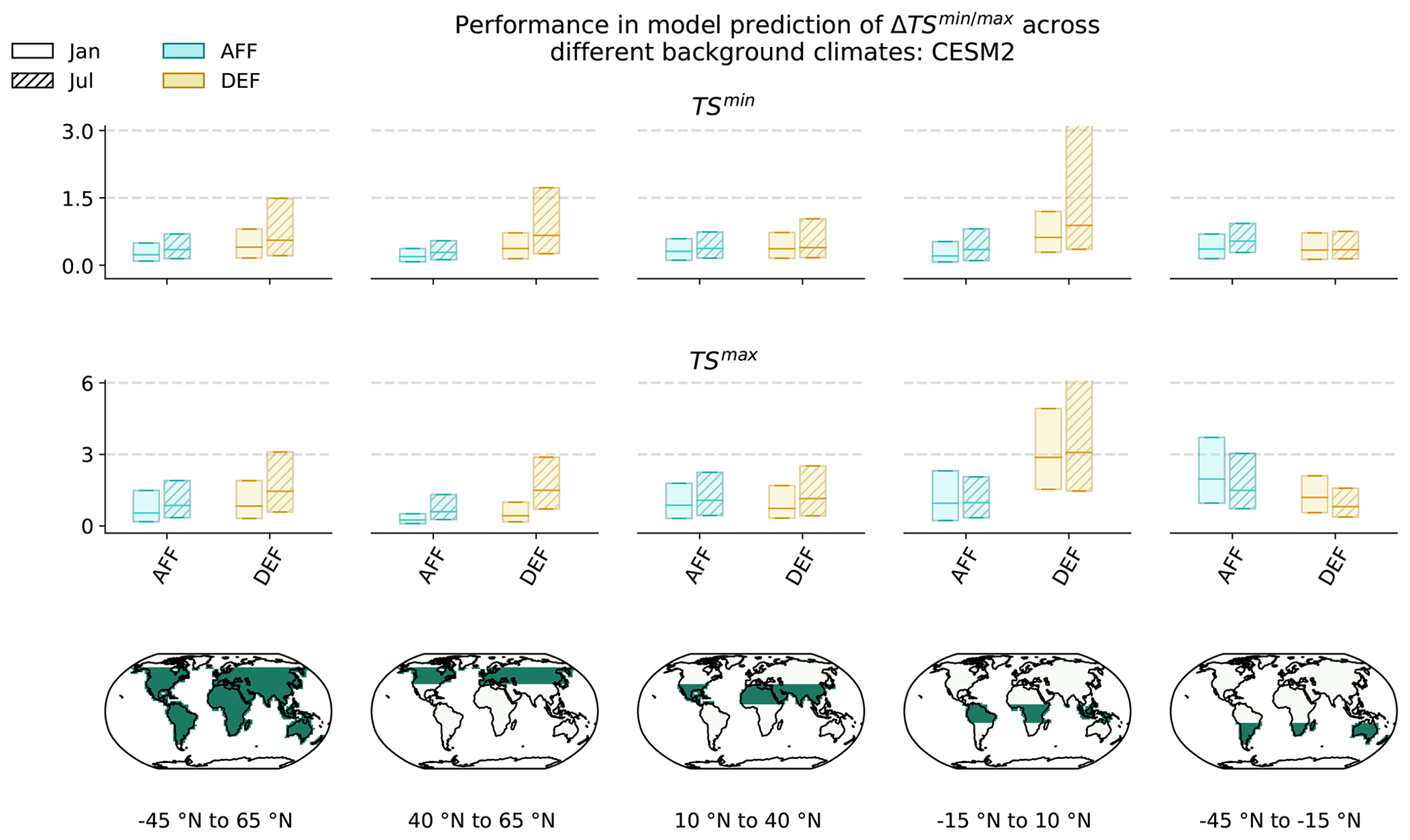
Figure C3Same as Fig. 4 but for CESM2, TSmin, and TSmax.
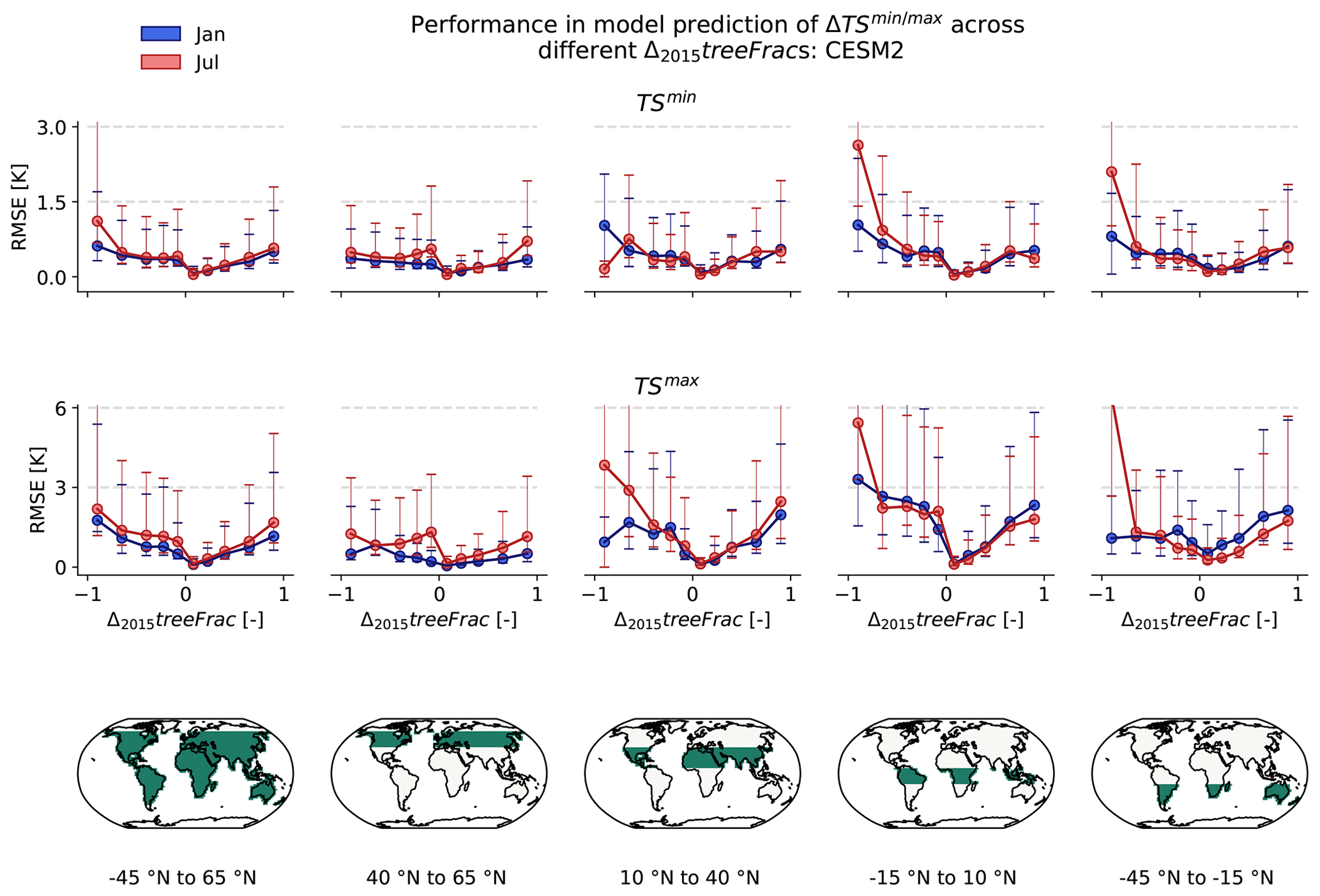
Figure C4Same as Fig. 5 but for CESM2, TSmin, and TSmax.
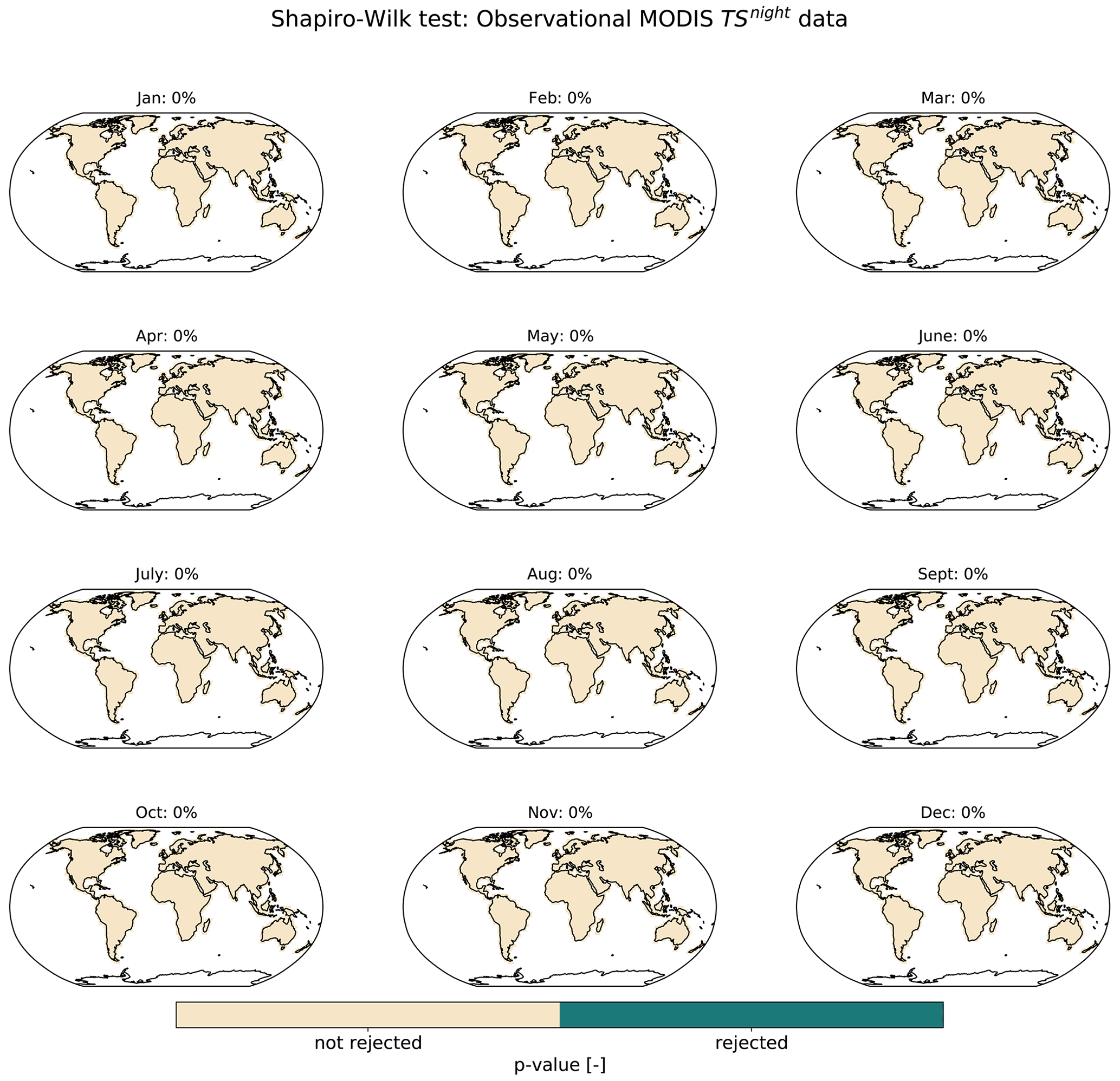
Figure D1Shapiro–Wilk test for normality of TSnight observational data obtained by the MODIS satellite. The null hypothesis is that the residuals are normally distributed. A Benjamini–Hochberg multiple-test correction (Benjamini and Hochberg, 1995) is applied to the p values before plotting them. Percentage values indicate the proportion of grid points for which the null hypothesis is rejected.
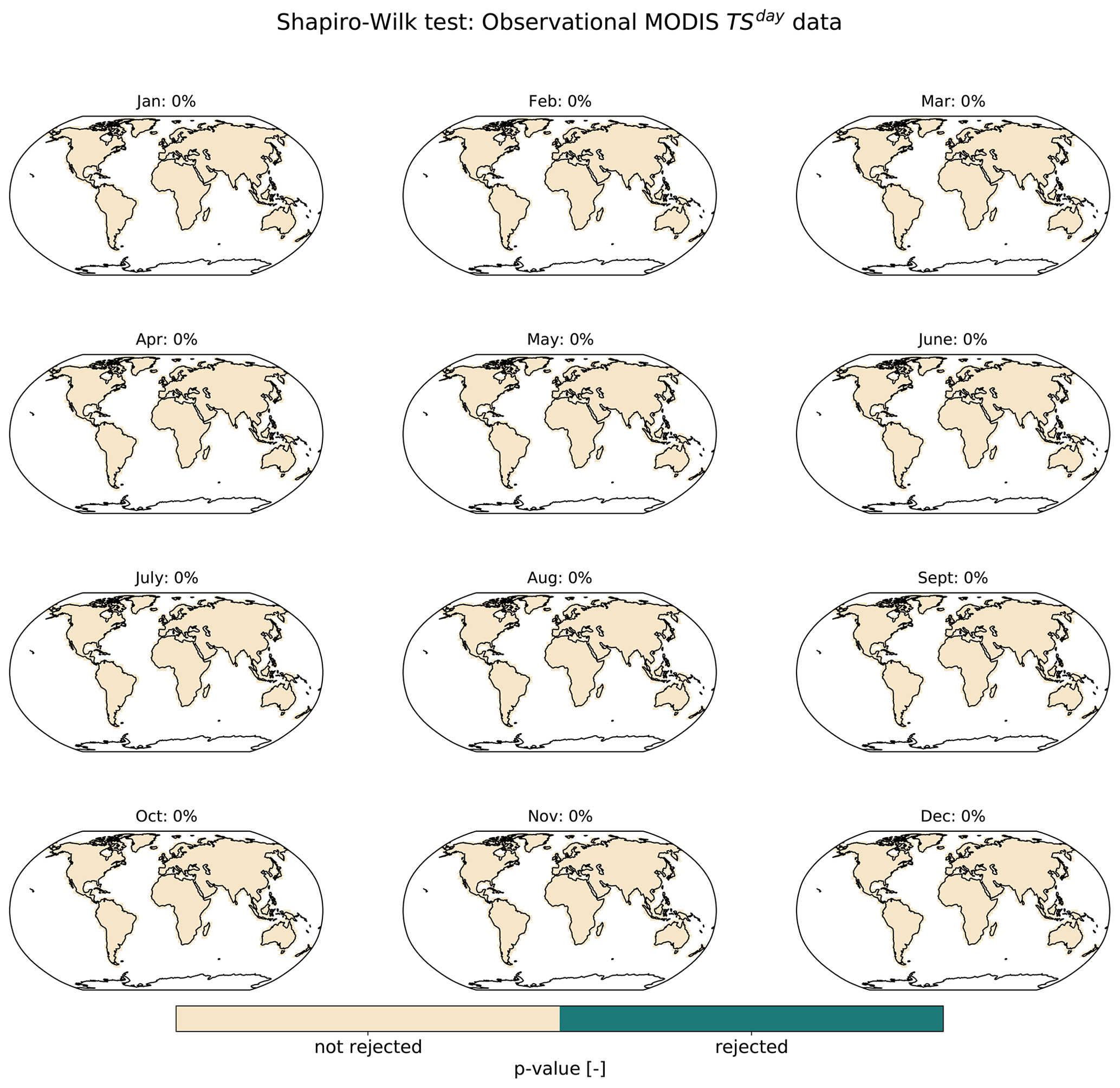
Figure D2Same as Fig. D1 but for TSday observational data obtained by the MODIS satellite.
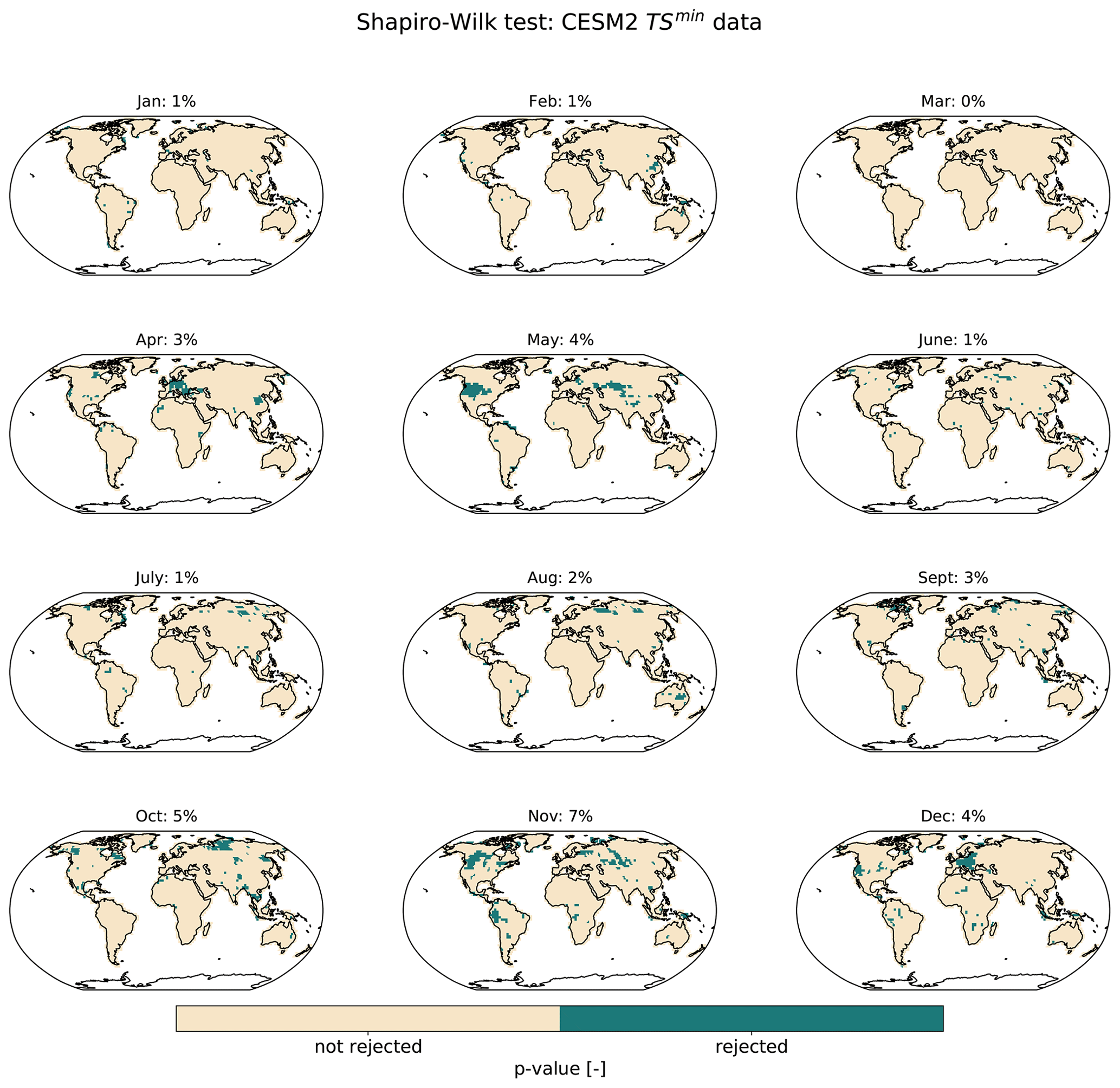
Figure D3Same as Fig. D1 but for TSmin data obtained from CESM2.
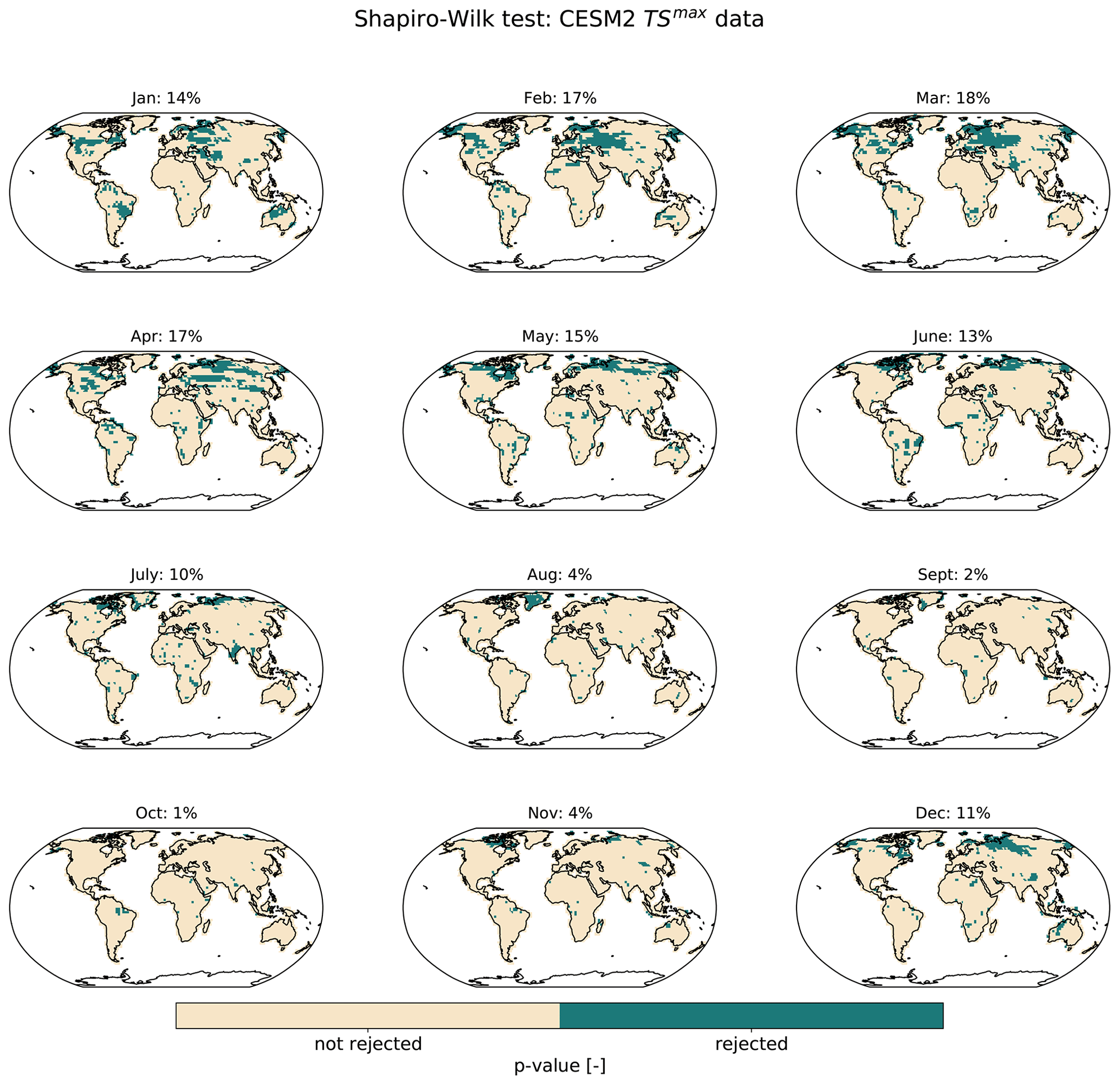
Figure D4Same as Fig. D1 but for TSmax data obtained from CESM2.
Data from the LAMACLIMA ESM experiments are archived on Zenodo under the link https://doi.org/10.5281/zenodo.7261374 (Nath et al., 2022a). Observational data used are available at Figshare https://doi.org/10.6084/m9.figshare.c.3829333.v1; see Duveiller et al. (2018d). The code used for the emulator calibration, evaluation, and sampling is archived on Zenodo under the link https://doi.org/10.5281/Zenodo.7261281 (Nath, 2022).
QL, CFS, and SIS identified the need for an emulator framework applied to representing land-cover-forced climate responses. SN developed the emulator set-up and the calibration and evaluation procedure with help from QL, LG ,and JS. QL and GD furthermore assisted SN in integrating the observationally based 2 m air temperature diagnosis scheme within the emulator. SJDH, QL, FH, FL, IM, JP, and WT produced the ESM output. All the authors contributed to interpreting the results and streamlining the text.
The contact author has declared that none of the authors has any competing interests.
Publisher’s note: Copernicus Publications remains neutral with regard to jurisdictional claims in published maps and institutional affiliations.
The authors wish to thank members of the Work Package 1 of the LAMACLIMA project for running and providing the ESM training data. Steven De Hertog, Wim Thiery, and Felix Havermann should particularly be acknowledged for their help in interpreting the LAMACLIMA outputs. Furthermore, we are grateful to Edouard Davin for providing guidance in designing the emulator.
This research has been supported by the LAMACLIMA project, which is part of AXIS, an ERA-NET initiated by JPI Climate and funded by DLR/BMBF (DE, grant no. 01LS1905A), NWO (NL), RCN (NO), and BELSPO (BE) with co-funding from the European Union (grant no. 776608), and the European Research Council, within the framework of the H2020 EXCELLENT SCIENCE proof-of-concept project MESMER-X (project no. 964013). Gregory Duveiller acknowledges funding from the European Research Council (ERC) Synergy Grant “Understanding and Modelling the Earth System with Machine Learning (USMILE)” under the Horizon 2020 Research and Innovation programme (grant agreement no. 855187).
This paper was edited by Christoph Müller and reviewed by two anonymous referees.
Alexeeff, S. E., Nychka, D., Sain, S. R., and Tebaldi, C.: Emulating mean patterns and variability of temperature across and within scenarios in anthropogenic climate change experiments, Climatic Change, 146, 319–333, https://doi.org/10.1007/s10584-016-1809-8, 2018. a
Benjamini, Y. and Hochberg, Y.: benjamini_hochberg1995, J. Roy. Stat. Soc. B, 57, 289–300, 1995. a
Beusch, L., Gudmundsson, L., and Seneviratne, S. I.: Emulating Earth system model temperatures with MESMER: from global mean temperature trajectories to grid-point-level realizations on land, Earth Syst. Dynam., 11, 139–159, https://doi.org/10.5194/esd-11-139-2020, 2020. a, b
Boisier, J. P., De Noblet-Ducoudré, N., Pitman, A. J., Cruz, F. T., Delire, C., Van Den Hurk, B. J., Van Der Molen, M. K., Mller, C., and Voldoire, A.: Attributing the impacts of land-cover changes in temperate regions on surface temperature and heat fluxes to specific causes: Results from the first LUCID set of simulations, J. Geophys. Res.-Atmos., 117, 1–16, https://doi.org/10.1029/2011JD017106, 2012. a
Boysen, L. R., Brovkin, V., Pongratz, J., Lawrence, D. M., Lawrence, P., Vuichard, N., Peylin, P., Liddicoat, S., Hajima, T., Zhang, Y., Rocher, M., Delire, C., Séférian, R., Arora, V. K., Nieradzik, L., Anthoni, P., Thiery, W., Laguë, M. M., Lawrence, D., and Lo, M.-H.: Global climate response to idealized deforestation in CMIP6 models, Biogeosciences, 17, 5615–5638, https://doi.org/10.5194/bg-17-5615-2020, 2020. a, b
Brunner, L., Hauser, M., Lorenz, R., and Beyerle, U.: The ETH Zurich CMIP6 next generation archive: technical documentation, Zenodo, https://doi.org/10.5281/zenodo.3734128, 2020. a
Calvin, K. and Bond-Lamberty, B.: Integrated human-earth system modeling – State of the science and future directions, Environ. Res. Lett., 13, 6, https://doi.org/10.1088/1748-9326/aac642, 2018. a
Castruccio, S., Hu, Z., Sanderson, B., Karspeck, A., and Hammerling, D.: Reproducing internal variability with few ensemble runs, J. Climate, 32, 8511–8522, https://doi.org/10.1175/JCLI-D-19-0280.1, 2019. a
COP: Glasgow leaders' declaration on forest and land-use, https://ukcop26.org/glasgow-leaders-declaration-on-forests-and-land-use/ (last access: 6 June 2022), 2021. a
Davin, E. L., Rechid, D., Breil, M., Cardoso, R. M., Coppola, E., Hoffmann, P., Jach, L. L., Katragkou, E., de Noblet-Ducoudré, N., Radtke, K., Raffa, M., Soares, P. M. M., Sofiadis, G., Strada, S., Strandberg, G., Tölle, M. H., Warrach-Sagi, K., and Wulfmeyer, V.: Biogeophysical impacts of forestation in Europe: first results from the LUCAS (Land Use and Climate Across Scales) regional climate model intercomparison, Earth Syst. Dynam., 11, 183–200, https://doi.org/10.5194/esd-11-183-2020, 2020. a, b
De Hertog, S. J., Havermann, F., Vanderkelen, I., Guo, S., Luo, F., Manola, I., Coumou, D., Davin, E. L., Duveiller, G., Lejeune, Q., Pongratz, J., Schleussner, C.-F., Seneviratne, S. I., and Thiery, W.: The biogeophysical effects of idealized land cover and land management changes in Earth system models, Earth Syst. Dynam., 13, 1305–1350, https://doi.org/10.5194/esd-13-1305-2022, 2022. a, b, c, d, e, f
De Noblet-Ducoudré, N., Boisier, J. P., Pitman, A., Bonan, G. B., Brovkin, V., Cruz, F., Delire, C., Gayler, V., Van Den Hurk, B. J., Lawrence, P. J., Van Der Molen, M. K., Müller, C., Reick, C. H., Strengers, B. J., and Voldoire, A.: Determining robust impacts of land-use-induced land cover changes on surface climate over North America and Eurasia: Results from the first set of LUCID experiments, J. Climate, 25, 3261–3281, https://doi.org/10.1175/JCLI-D-11-00338.1, 2012. a, b
Duveiller, G., Forzieri, G., Robertson, E., Li, W., Georgievski, G., Lawrence, P., Wiltshire, A., Ciais, P., Pongratz, J., Sitch, S., Arneth, A., and Cescatti, A.: Biophysics and vegetation cover change: a process-based evaluation framework for confronting land surface models with satellite observations, Earth Syst. Sci. Data, 10, 1265–1279, https://doi.org/10.5194/essd-10-1265-2018, 2018a.
Duveiller, G., Hooker, J., and Cescatti, A.: The mark of vegetation change on Earth's surface energy balance, Nat. Commun., 9, 679, https://doi.org/10.1038/s41467-017-02810-8, 2018b. a
Duveiller, G., Hooker, J., and Cescatti, A.: A dataset mapping the potential biophysical effects of vegetation cover change, Sci. Data, 5, 1–15, https://doi.org/10.1038/sdata.2018.14, 2018c. a, b, c
Duveiller, G., Hooker, J., and Cescatti, A.: A dataset mapping the potential biophysical effects of vegetation cover change, figshare [data], https://doi.org/10.6084/m9.figshare.c.3829333.v1, 2018d. a
Efron, B. and Tibshirani, R. J.: An Introduction to the Bootstrap, in: An Introduction to the Bootstrap, Chapman and Hall/CRC, https://doi.org/10.1201/9780429246593, 1993. a
Fujimori, S., Hasegawa, T., Masui, T., Takahashi, K., Herran, D. S., Dai, H., Hijioka, Y., and Kainuma, M.: SSP3: AIM implementation of Shared Socioeconomic Pathways, Global Environ. Chang., 42, 268–283, https://doi.org/10.1016/j.gloenvcha.2016.06.009, 2017. a
Hastie, T. and Tibshirani, R.: Generalized additive models, Stat. Sci., 1, 297–318, 1986. a, b
Hastie, T. and Tibshirani, R.: Varying Coefficients Model, J. Roy. Stat. Soc. B, 55, 757–796, 1993. a
Hirsch, A. L., Guillod, B. P., Seneviratne, S. I., Beyerle, U., Boysen, L. R., Brovkin, V., Davin, E. L., Doelman, J. C., Kim, H., Mitchell, D. M., Nitta, T., Shiogama, H., Sparrow, S., Stehfest, E., van Vuuren, D. P., and Wilson, S.: Biogeophysical Impacts of Land-Use Change on Climate Extremes in Low-Emission Scenarios: Results From HAPPI-Land, Earth's Future, 6, 396–409, https://doi.org/10.1002/2017EF000744, 2018. a
Hooker, J., Duveiller, G., and Cescatti, A.: Data descriptor: A global dataset of air temperature derived from satellite remote sensing and weather stations, Sci. Data, 5, 1–11, https://doi.org/10.1038/sdata.2018.246, 2018. a, b, c, d, e, f, g, h, i, j, k, l, m, n, o, p, q, r, s, t, u, v, w, x
Lawrence, D., Coe, M., Walker, W., Verchot, L., and Vandecar, K.: The Unseen Effects of Deforestation: Biophysical Effects on Climate, Frontiers in Forests and Global Change, 5, 1–13, https://doi.org/10.3389/ffgc.2022.756115, 2022. a
Lawrence, D. M., Hurtt, G. C., Arneth, A., Brovkin, V., Calvin, K. V., Jones, A. D., Jones, C. D., Lawrence, P. J., de Noblet-Ducoudré, N., Pongratz, J., Seneviratne, S. I., and Shevliakova, E.: The Land Use Model Intercomparison Project (LUMIP) contribution to CMIP6: rationale and experimental design, Geosci. Model Dev., 9, 2973–2998, https://doi.org/10.5194/gmd-9-2973-2016, 2016. a, b
Lejeune, Q., Davin, E. L., Gudmundsson, L., Winckler, J., and Seneviratne, S. I.: Historical deforestation locally increased the intensity of hot days in northern mid-latitudes, Nat. Clim. Change, 8, 386–390, https://doi.org/10.1038/s41558-018-0131-z, 2018. a, b
Li, Y., Zhao, M., Motesharrei, S., Mu, Q., Kalnay, E., and Li, S.: Local cooling and warming effects of forests based on satellite observations, Nat. Commun., 6, 6603, https://doi.org/10.1038/ncomms7603, 2015. a
Link, R., Snyder, A., Lynch, C., Hartin, C., Kravitz, B., and Bond-Lamberty, B.: Fldgen v1.0: an emulator with internal variability and space–time correlation for Earth system models, Geosci. Model Dev., 12, 1477–1489, https://doi.org/10.5194/gmd-12-1477-2019, 2019. a
Luyssaert, S., Jammet, M., Stoy, P. C., Estel, S., Pongratz, J., Ceschia, E., Churkina, G., Don, A., Erb, K., Ferlicoq, M., Gielen, B., Grünwald, T., Houghton, R. A., Klumpp, K., Knohl, A., Kolb, T., Kuemmerle, T., Laurila, T., Lohila, A., Loustau, D., McGrath, M. J., Meyfroidt, P., Moors, E. J., Naudts, K., Novick, K., Otto, J., Pilegaard, K., Pio, C. A., Rambal, S., Rebmann, C., Ryder, J., Suyker, A. E., Varlagin, A., Wattenbach, M., and Dolman, A. J.: Land management and land-cover change have impacts of similar magnitude on surface temperature, Nat. Clim. Change, 4, 389–393, https://doi.org/10.1038/nclimate2196, 2014. a
McKinnon, K. A. and Deser, C.: Internal variability and regional climate trends in an observational large ensemble, J. Climate, 31, 6783–6802, https://doi.org/10.1175/JCLI-D-17-0901.1, 2018. a
Meier, R., Davin, E. L., Lejeune, Q., Hauser, M., Li, Y., Martens, B., Schultz, N. M., Sterling, S., and Thiery, W.: Evaluating and improving the Community Land Model's sensitivity to land cover, Biogeosciences, 15, 4731–4757, https://doi.org/10.5194/bg-15-4731-2018, 2018. a, b
Menne, M. J., Williams, C. N., Gleason, B. E., Rennie, J. J., and Lawrimore, J. H.: The Global Historical Climatology Network Monthly Temperature Dataset, Version 4, J. Climate, 31, 9835–9854, https://doi.org/10.1175/JCLI-D-18-0094.1, 2018. a
Nath, S.: snath-xoc/TIMBER-v0.1_Nath_et_al_2022: TIMBER, Zenodo [code], https://doi.org/10.5281/zenodo.7261281, 2022. a
Nath, S., Hertog, S. J. D., Guo, S., Havermann, F., Luo, F., Manola, I., Pongratz, J., and Thiery, W.: LAMACLIMA_experiments_for_training_TIMBERv0.1, Zenodo [data], https://doi.org/10.5281/zenodo.7261374, 2022a. a
Nath, S., Lejeune, Q., Beusch, L., Seneviratne, S. I., and Schleussner, C.-F.: MESMER-M: an Earth system model emulator for spatially resolved monthly temperature, Earth Syst. Dynam., 13, 851–877, https://doi.org/10.5194/esd-13-851-2022, 2022b. a, b
Pitman, A. J., de Noblet-Ducoudré, N., Avila, F. B., Alexander, L. V., Boisier, J.-P., Brovkin, V., Delire, C., Cruz, F., Donat, M. G., Gayler, V., van den Hurk, B., Reick, C., and Voldoire, A.: Effects of land cover change on temperature and rainfall extremes in multi-model ensemble simulations, Earth Syst. Dynam., 3, 213–231, https://doi.org/10.5194/esd-3-213-2012, 2012. a
Popp, A., Calvin, K., Fujimori, S., Havlik, P., Humpenöder, F., Stehfest, E., Bodirsky, B. L., Dietrich, J. P., Doelmann, J. C., Gusti, M., Hasegawa, T., Kyle, P., Obersteiner, M., Tabeau, A., Takahashi, K., Valin, H., Waldhoff, S., Weindl, I., Wise, M., Kriegler, E., Lotze-Campen, H., Fricko, O., Riahi, K., and Vuuren, D. P.: Land-use futures in the shared socio-economic pathways, Global Environ. Chang., 42, 331–345, https://doi.org/10.1016/j.gloenvcha.2016.10.002, 2017. a, b
Quilcaille, Y., Gudmundsson, L., Beusch, L., Hauser, M., and Seneviratne, S. I.: Showcasing MESMER-X: Spatially resolved emulation of annual maximum temperatures of Earth System Models, Geophys. Res. Lett., 49, 1–11, https://doi.org/10.1029/2022GL099012, 2022. a
Riahi, K., van Vuuren, D. P., Kriegler, E., Edmonds, J., O'Neill, B. C., Fujimori, S., Bauer, N., Calvin, K., Dellink, R., Fricko, O., Lutz, W., Popp, A., Cuaresma, J. C., KC, S., Leimbach, M., Jiang, L., Kram, T., Rao, S., Emmerling, J., Ebi, K., Hasegawa, T., Havlik, P., Humpenöder, F., Da Silva, L. A., Smith, S., Stehfest, E., Bosetti, V., Eom, J., Gernaat, D., Masui, T., Rogelj, J., Strefler, J., Drouet, L., Krey, V., Luderer, G., Harmsen, M., Takahashi, K., Baumstark, L., Doelman, J. C., Kainuma, M., Klimont, Z., Marangoni, G., Lotze-Campen, H., Obersteiner, M., Tabeau, A., and Tavoni, M.: The Shared Socioeconomic Pathways and their energy, land use, and greenhouse gas emissions implications: An overview, Global Environ. Chang., 42, 153–168, https://doi.org/10.1016/j.gloenvcha.2016.05.009, 2017. a, b
Roberts, D. R., Bahn, V., Ciuti, S., Boyce, M. S., Elith, J., Guillera-Arroita, G., Hauenstein, S., Lahoz-Monfort, J. J., Schröder, B., Thuiller, W., Warton, D. I., Wintle, B. A., Hartig, F., and Dormann, C. F.: Cross-validation strategies for data with temporal, spatial, hierarchical, or phylogenetic structure, Ecography, 40, 913–929, https://doi.org/10.1111/ecog.02881, 2017. a, b, c
Seddon, N., Sengupta, S., Hauler, I., and Rizvi, A. R.: Nature-based solutions in nationally determined contributions, IUCN Library System, https://portals.iucn.org/library/node/48525 (last access: 6 June 2022), 2020. a
Seneviratne, S. I., Wartenburger, R., Guillod, B. P., Hirsch, A. L., Vogel, M. M., Brovkin, V., Van Vuuren, D. P., Schaller, N., Boysen, L., Calvin, K. V., Doelman, J., Greve, P., Havlik, P., Humpenöder, F., Krisztin, T., Mitchell, D., Popp, A., Riahi, K., Rogelj, J., Schleussner, C. F., Sillmann, J., and Stehfest, E.: Climate extremes, land-climate feedbacks and land-use forcing at 1.5C, Philos. T. Roy. Soc. A, 376, 2119, https://doi.org/10.1098/rsta.2016.0450, 2018. a
Thiery, W., Davin, E. L., Lawrence, D. M., Hirsch, A. L., Hauser, M., and Seneviratne, S. I.: Present-day irrigation mitigates heat extremes, J. Geophys. Res., 122, 1403–1422, https://doi.org/10.1002/2016JD025740, 2017. a
Thiery, W., Visser, A. J., Fischer, E. M., Hauser, M., Hirsch, A. L., Lawrence, D. M., Lejeune, Q., Davin, E. L., and Seneviratne, S. I.: Warming of hot extremes alleviated by expanding irrigation, Nat. Commun., 11, 290, https://doi.org/10.1038/s41467-019-14075-4, 2020. a
Van Vuuren, D. P., Batlle Bayer, L., Chuwah, C., Ganzeveld, L., Hazeleger, W., Van Den Hurk, B., Van Noije, T., Oneill, B., and Strengers, B. J.: A comprehensive view on climate change: Coupling of earth system and integrated assessment models, Environ. Res. Lett., 7, 2, https://doi.org/10.1088/1748-9326/7/2/024012, 2012. a
van Vuuren, D. P., Stehfest, E., Gernaat, D. E., Doelman, J. C., van den Berg, M., Harmsen, M., de Boer, H. S., Bouwman, L. F., Daioglou, V., Edelenbosch, O. Y., Girod, B., Kram, T., Lassaletta, L., Lucas, P. L., van Meijl, H., Müller, C., van Ruijven, B. J., van der Sluis, S., and Tabeau, A.: Energy, land-use and greenhouse gas emissions trajectories under a green growth paradigm, Global Environ. Chang., 42, 237–250, https://doi.org/10.1016/j.gloenvcha.2016.05.008, 2017. a
Winckler, J., Reick, C. H., and Pongratz, J.: Robust identification of local biogeophysical effects of land-cover change in a global climate model, J. Climate, 30, 1159–1176, https://doi.org/10.1175/JCLI-D-16-0067.1, 2017a. a
Winckler, J., Reick, C. H., and Pongratz, J.: Why does the locally induced temperature response to land cover change differ across scenarios?, Geophys. Res. Lett., 44, 3833–3840, https://doi.org/10.1002/2017GL072519, 2017b. a
Winckler, J., Reick, C. H., and Pongratz, J.: Robust identification of local biogeophysical effects of land-cover change in a global climate model, J. Climate, 30, 1159–1176, https://doi.org/10.1175/JCLI-D-16-0067.1, 2017c. a
Windisch, M. G., Davin, E. L., and Seneviratne, S. I.: Prioritizing forestation based on biogeochemical and local biogeophysical impacts, Nat. Clim. Change, 11, 867–871, https://doi.org/10.1038/s41558-021-01161-z, 2021. a
Wood, S. N.: Generalized Additive Models, Chapman and Hall/CRC, https://doi.org/10.1201/9781315370279, 2017. a, b, c, d
Yee, T. W. and Stephenson, A. G.: Vector generalized linear and additive extreme value models, Extremes, 10, 1–19, https://doi.org/10.1007/s10687-007-0032-4, 2007. a