Data space inversion for efficient uncertainty quantification using an integrated surface and sub-surface hydrologic model

It is incumbent on decision-support hydrological modelling to make predictions of uncertain quantities in a decision-support context. In implementing decision-support modelling, data assimilation and uncertainty quantification are often the most difficult and time-consuming tasks. This is because the imposition of history-matching constraints on model parameters usually requires a large number of model runs. Data space inversion (DSI) provides a highly model-run-efficient method for predictive uncertainty quantification. It does this by evaluating covariances between model outputs used for history matching (e.g. hydraulic heads) and model predictions based on model runs that sample the prior parameter probability distribution. By directly focusing on the relationship between model outputs under historical conditions and predictions of system behaviour under future conditions, DSI avoids the need to estimate or adjust model parameters. This is advantageous when using integrated surface and sub-surface hydrologic models (ISSHMs) because these models are associated with long run times, numerical instability and ideally complex parameterization schemes that are designed to respect geological realism. This paper demonstrates that DSI provides a robust and efficient means of quantifying the uncertainties of complex model predictions. At the same time, DSI provides a basis for complementary linear analysis that allows the worth of available observations to be explored, as well as of observations which are yet to be acquired. This allows for the design of highly efficient, future data acquisition campaigns. DSI is applied in conjunction with an ISSHM representing a synthetic but realistic river–aquifer system. Predictions of interest are fast travel times and surface water infiltration. Linear and non-linear estimates of predictive uncertainty based on DSI are validated against a more traditional uncertainty quantification which requires the adjustment of a large number of parameters. A DSI-generated surrogate model is then used to investigate the effectiveness and efficiency of existing and possible future monitoring networks. The example demonstrates the benefits of using DSI in conjunction with a complex numerical model to quantify predictive uncertainty and support data worth analysis in complex hydrogeological environments.

1 Introduction

Numerical hydrological models are often built to make predictions that support decision-making. In this paper we use the term “prediction” to refer to any quantity of management interest calculated by a numerical model, whether it is estimated in the future or is a by-product of data assimilation. Generally, Bayesian methods are applied to models so that the uncertainties associated with predictions of management interest can be quantified and reduced. Through this process, the prior uncertainties of these predictions are constrained by the assimilation of observations to provide estimates of posterior predictive uncertainties. A variety of Bayesian methods are available for this purpose. These include linear methods (James et al., 2009; Dausman et al., 2010), linear-assisted methods such as null-space Monte Carlo (Tonkin and Doherty, 2009; Doherty, 2015) and non-linear methods such Markov chain Monte Carlo (see, for example, Vrugt, 2016). More recently, ensemble methods such as those described by Chen and Oliver (2013) and White (2018) have been used in this context. The attractiveness of ensemble methods lies in their ability to accommodate a large number of parameters with a high degree of model run efficiency.

In many hydrogeological settings, geological structures such as elongate structural or alluvial features that embody interconnected permeability are of high conceptual relevance as they can have a major impact on management-salient predictions. Representation of these features typically requires the use of categorical parameterization schemes that maintain their relation and connectivity in space. Despite the efficiency of ensemble methods, it is difficult for them to adjust and maintain permeability connectedness as parameter fields are adjusted so that model outputs can respect field measurements (Lam et al., 2020; Juda et al., 2023). Additionally, theoretical problems arise from the multi-Gaussian assumption on which ensemble methods are based. Practical problems arise from the sometimes problematic behaviour of complex numerical models when endowed with stochastic parameter fields with high contrasts in hydraulic conductivity. These problems are generally exacerbated when solute transport is simulated in addition to flow. It follows that the use of model partner software such as PEST (Doherty, 2022) and PESTPP-IES (White, 2018) for parameter field conditioning and predictive uncertainty analysis and reduction is not always feasible. This makes it difficult to maintain the simulation integrity of physically based numerical models where potentially information-rich site data must be assimilated. Compromises in model structure, parameterization or process complexity may therefore be required (see, for example, Delottier et al., 2022).

To overcome these problems, methods have been developed to generate posterior distributions of predictions without the need to adjust the complex parameter fields of large, physically based numerical models (for example Satija and Caers, 2015; He et al., 2018; Hermans, 2017; Sun and Durlofsky, 2017). Computational advantages are gained by establishing a direct link between historical observations of system behaviour and predictions of interest. To establish this link, a numerical model of arbitrary process complexity is used. This model is equipped with parameter fields that can best express the hydrogeological characteristics of the simulated system. These may include complex structures that represent heterogeneous, three-dimensional configurations of hydraulic properties. Because no adjustment of the parameter fields is required, simulation integrity is maintained regardless of the complexity of hydrogeological site conceptualization. Instead, the model is used to build a prior probability distribution of predictions of interest based on samples of realistic hydraulic property fields. The same model runs that are used to explore prior predictive uncertainty are used to construct a joint probability distribution that links historical system behaviour with future system behaviour.

Some of the methods that adopt this approach to posterior predictive uncertainty analysis attempt to develop explicit relationships between historical observations of system behaviour on the one hand and predictions of future system behaviour on the other hand (Satija and Caers, 2015; Scheidt et al., 2015). In contrast, other methods develop a more implicit relationship between these two (Sun and Durlofsky, 2017; Lima et al., 2020). Once these relationships have been established, predictions of interest can be directly conditioned by real-world measurements of historical system behaviour. The need for manipulation and estimation of parameters is thereby obviated. Consequently, the numerical burden of predictive uncertainty reduction and quantification is significantly reduced, regardless of the complexity of the numerical model and regardless of the complexity of the prior parameter probability distribution.

In this paper, we employ a “data space inversion” (i.e. DSI) methodology that is similar to that described by Lima et al. (2020). At the same time, we extend the methodology to consider the worth of existing and future data. Assessment of data worth is based on the premise that the value of data increases with its ability to reduce the uncertainties of predictions. Because it requires uncertainty quantification, assessing the worth of data using methods that rely on explicit or implicit (through linear analysis) parameter adjustment can be computationally expensive, especially when performed in numerical and parameterization contexts that attempt to respect hydrogeological processes and hydraulic property integrity. The numerically inexpensive methodology for data worth assessment that is presented herein can support these assessments in modelling contexts where it would otherwise be computationally intractable. The proposed approach is therefore especially attractive for integrated surface and sub-surface hydrologic models (ISSHMs). Thus it can support attempts to achieve the goals of decision-support utility and failure avoidance that are set out in articles such as Kikuchi (2017) and Doherty and Moore (2020).

All of the methods described here can be applied using PEST (Doherty, 2022) and PEST$++$ (PEST$++$ Development Team, 2022). They are therefore readily available to the wider modelling community.

The paper is organized as follows: Sect. 2 describes the theory behind DSI. In the ensuing section, a synthetic alluvial river–aquifer system is introduced. This is then used to (i) validate DSI estimates of predictive uncertainty and (ii) demonstrate the use of DSI in quantifying the worth of existing and new data in reducing predictive uncertainty.

2 Theory

2.1 Statistical linkage between the past and the future

Let the vector o denote outputs of a model that correspond to field measurements of system behaviour (e.g. system states and fluxes). Meanwhile, we denote the actual field measurements of these quantities by the vector h. We use the symbol Z to characterize the operator through which model outputs o are calculated from model parameters; the latter are denoted by the vector k. Therefore,

$$\begin{array}{}\text{(1)}& \mathit{h}=\mathit{o}+\mathit{\epsilon }=\mathbf{Z}\left(\mathit{k}\right)+\mathit{\epsilon }.\end{array}$$

The vector ε denotes the noise associated with field measurements h. It may also include the model-to-measurement misfit which arises from the imperfect nature of numerical simulation. In the present case we combine both of these into a single “noise” term. It is generally assumed that ε has a mean of 0; we denote its covariance matrix by C(ε).

Ideally, k in Eq. (1) can represent any model inputs that are incompletely known. Conceptually, there is no limit to the number of elements that comprise the vector k and hence to the complexity of model parameterization. Typically, elements of k represent spatially distributed hydraulic and transport properties. They may also include historical system stresses, such as pumping and recharge rates that are poorly estimated, as well as some uncertain specifications of other boundary conditions.

Suppose the model is run over a period for which predictions are made. Let the vector s contain simulator predictions of interest. We depict these as being computed from model parameters using the operator Y. Thus,

$$\begin{array}{}\text{(2)}& \mathit{s}=\mathbf{Y}\left(\mathit{k}\right).\end{array}$$

Suppose that the model is run N times over its simulation period and that this simulation period spans both the time over which history matching is performed (that is, the “calibration period”) and the time over which predictions are required (that is, the “prediction period”); depending on the prediction, these two periods may coincide. Suppose further that on each of the N occasions on which the model is run, the vector k comprises a different sample of its prior probability distribution. The set of N realizations of o computed by the model over these N model realizations can be collected into a matrix O by arranging them in columns. Meanwhile, the set of N realizations of s in Eq. (2) can be similarly collected into a matrix S. From these realizations, vectors depicting the mean of O and the mean of S (i.e. o and s) are calculated as

$$\begin{array}{}\text{(3a)}& {\displaystyle }\underset{\mathrm{¯}}{\mathit{o}}={\displaystyle \frac{{\sum }_{i=\mathrm{1}}^N{\mathit{o}}_i}{N}},\text{(3b)}& {\displaystyle }\underset{\mathrm{¯}}{\mathit{s}}={\displaystyle \frac{{\sum }_{i=\mathrm{1}}^N{\mathit{s}}_i}{N}},\end{array}$$

where o_i and s_i in Eq. (3a) and (3b) depict the ith column of O and S, respectively. Let O and S designate matrices whose columns are comprised of replicates of o and s. Consider now the covariance matrix:

$$\begin{array}{}\text{(4)}& C\left(\left[\begin{array}{c}\mathit{o}\\ \mathit{s}\end{array}\right]\right)=\left[\begin{array}{cc}{C}_{\text{oo}}& C_{\text{os}}\\ C_{\text{so}}& C_{\text{ss}}\end{array}\right],\end{array}$$

where

$$\begin{array}{}\text{(5a)}& {\displaystyle }{C}_{\text{oo}}={\displaystyle \frac{\left(\mathbf{O}-\underset{\mathrm{¯}}{\mathbf{O}}\right){\left(\mathbf{O}-\underset{\mathrm{¯}}{\mathbf{O}}\right)}^{\mathrm{T}}}{N-\mathrm{1}}},\text{(5b)}& {\displaystyle }{C}_{\text{os}}=C_{\text{so}}^{\mathrm{T}}={\displaystyle \frac{\left(\mathbf{O}-\underset{\mathrm{¯}}{\mathbf{O}}\right){\left(\mathbf{S}-\underset{\mathrm{¯}}{\mathbf{S}}\right)}^{\mathrm{T}}}{N-\mathrm{1}}},\text{(5c)}& {\displaystyle }{C}_{\text{ss}}={\displaystyle \frac{\left(\mathbf{S}-\underset{\mathrm{¯}}{\mathbf{S}}\right){\left(\mathbf{S}-\underset{\mathrm{¯}}{\mathbf{S}}\right)}^{\mathrm{T}}}{N-\mathrm{1}}}.\end{array}$$

Submatrices appearing on the right side of Eq. (4) can be calculated from realizations of model outputs using Eq. (5a), (5b) and (5c).

Conditioning of predictions by historical observations of system state (see below) often benefits from transforming individual elements o_i and s_i of o and s into normally distributed variables $o_i^{\mathrm{g}}$ and $s_i^{\mathrm{g}}$ before calculating the covariance matrices that are depicted in Eq. (4). Unfortunately, Gaussian transformation of individual elements of o and s does not guarantee that the joint probability distribution of [o^gT,s^gT] is multi-Gaussian. However, this can be at least partially accommodated by undertaking an ensemble-based conditioning process in which o^g and s^g are linked by a surrogate model. This is now discussed. Meanwhile, to make the following notations a little less complex, we drop the “g” superscript.

2.2 The DSI surrogate model

Sun and Durlofsky (2017) and Lima et al. (2020) demonstrate the use of a covariance-matrix-derived surrogate model that can be used to link o and s. Conditioning of s by h (the measured counterpart of o) is then achieved by adjusting the parameters of this model using standard parameter conditioning methodologies. The former authors use the randomized maximum likelihood method, while the latter authors use an ensemble smoother.

The DSI prediction model is described by the following equation:

$$\begin{array}{}\text{(6)}& \left[\begin{array}{c}\mathit{o}\\ \mathit{s}\end{array}\right]=\left[\begin{array}{c}{\mathit{o}}_{\mathrm{p}}\\ {\mathit{s}}_{\mathrm{p}}\end{array}\right]+C^{\mathrm{1}/\mathrm{2}}\left(\left[\begin{array}{c}\mathit{o}\\ \mathit{s}\end{array}\right]\right)\mathit{x}.\end{array}$$

“Adjustable parameters” of this model comprise the vector x in Eq. (6). Meanwhile o_p and s_p are prior mean values of o and s. The prior probability distribution of elements x_i of x is such that they are independently normal with a standard deviation of 1.0. Thus,

$$\begin{array}{}\text{(7a)}& E\left(\mathit{x}\right)=\mathrm{0}\end{array}$$

and

$$\begin{array}{}\text{(7b)}& C\left(\mathit{x}\right)=\mathbf{I},\end{array}$$

where E(x) in Eq. (7a) denotes the expected value of x and C(x) in Eq. (7b) denotes the prior covariance matrix of x. The square root of the covariance matrix that is depicted in Eq. (6) is obtained using singular value decomposition. First,

$$\begin{array}{}\text{(8)}& C\left(\left[\begin{array}{c}\mathit{o}\\ \mathit{s}\end{array}\right]\right)=\mathbf{U}\mathbf{\Sigma }{\mathbf{U}}^{\mathrm{T}},\end{array}$$

where U in Eq. (8) is an orthonormal matrix and Σ is a diagonal matrix whose elements are positive singular values. The square root of this matrix is then obtained as

$$\begin{array}{}\text{(9)}& C^{\mathrm{1}/\mathrm{2}}\left(\left[\begin{array}{c}\mathit{o}\\ \mathit{s}\end{array}\right]\right)=\mathbf{U}{\mathbf{\Sigma }}^{\mathrm{1}/\mathrm{2}}{\mathbf{U}}^{\mathrm{T}}.\end{array}$$

Normally ${\mathbf{\Sigma }}^{\mathrm{1}/\mathrm{2}}$ in Eq. (9) is truncated so that unduly low singular values are excluded. The sum of squared singular values (i.e. the diagonal elements of ${\mathbf{\Sigma }}^{\mathrm{1}/\mathrm{2}}$) is a measure of the total variability in $\left[\begin{array}{c}\mathit{o}\\ \mathit{s}\end{array}\right]$. Normally truncation of ${\mathbf{\Sigma }}^{\mathrm{1}/\mathrm{2}}$ is such that 99 % or more of this variability is retained. Once singular value truncation has been accomplished, a linearized inverse problem can be formulated using the following Eq. (10). (Without loss of generality, we omit the vector of prior means $\left[\begin{array}{c}{\mathit{o}}_{\mathrm{p}}\\ {\mathit{s}}_{\mathrm{p}}\end{array}\right]$ in this and the following equations to simplify them.)

$$\begin{array}{}\text{(10)}& \left[\begin{array}{c}\mathit{h}\\ \mathit{s}\end{array}\right]=C^{\mathrm{1}/\mathrm{2}}\left(\left[\begin{array}{c}\mathit{o}\\ \mathit{s}\end{array}\right]\right)\mathit{x}+\left[\begin{array}{c}\mathit{\epsilon }\\ \mathit{0}\end{array}\right]=\mathbf{M}\mathit{x}+\left[\begin{array}{c}\mathit{\epsilon }\\ \mathit{0}\end{array}\right]\end{array}$$

The matrix operator M is defined through the above equation. Let the matrix N be an appropriate “selection matrix” comprised of 1s and 0s such that

$$\begin{array}{}\text{(11)}& \mathit{h}=\mathbf{N}\left[\begin{array}{c}\mathit{h}\\ \mathit{s}\end{array}\right].\end{array}$$

Then,

$$\begin{array}{}\text{(12)}& \mathit{h}=\mathbf{L}\mathit{x}+\mathit{\epsilon },\end{array}$$

where

$$\begin{array}{}\text{(13)}& \mathbf{L}=\mathbf{N}{C}^{\mathrm{1}/\mathrm{2}}\left(\left[\begin{array}{c}\mathit{o}\\ \mathit{s}\end{array}\right]\right).\end{array}$$

In Eqs. (10) to (12), the vector h contains measurements of historical system behaviour that correspond to model outputs o (same as in Eq. 1). We refer to the model M herein as the “DSI surrogate model” that links elements of observed system behaviour to elements of its predicted behaviour (normally those that have decision-relevance). As stated above, the former are encapsulated in the vector o, while the latter are encapsulated in the vector s. This surrogate model can be “calibrated” against field measurements of system state encapsulated in h to obtain a maximum a posteriori (MAP) estimate $\underset{\mathrm{¯}}{\mathit{x}}$ of x, from which a MAP estimate $\underset{\mathrm{¯}}{\mathit{s}}$ of s can be readily obtained using Eq. (6). Alternatively, or in addition, samples of the posterior distribution of x can be obtained using standard Bayesian methods. In the following analysis, we use an ensemble smoother as well as a linearized form of Bayes equation for prediction conditioning. Because the computations embodied in Eq. (10) are simple, the DSI surrogate model runs extremely fast.

2.3 Imposition of history-match constraints

In the examples that follow, we apply Eqs. (10) and (12) in a number of different ways. These will now be briefly described.

The first of these applications is similar to that described by Lima et al. (2020). That is, an ensemble smoother is used to directly sample the posterior probability distribution of x. The posterior probability distribution of s is then sampled by running the DSI surrogate model using these samples of x. We use the PESTPP-IES ensemble smoother described by the PEST$++$ development team (2022) for this purpose.

We then use Tikhonov-regularized inversion to “calibrate” the surrogate model, thereby obtaining a MAP estimate $\underset{\mathrm{¯}}{\mathit{x}}$ of x from which a MAP estimate $\underset{\mathrm{¯}}{\mathit{s}}$ of s is obtained from a single forward run of the calibrated DSI surrogate model. Calibration is achieved using PEST (Doherty, 2022). Because of Eq. (6) and the fact that the prior expected value of x is 0, the Tikhonov-regularized solution to the inverse problem described by Eq. (12) is (Doherty, 2015)

$$\begin{array}{}\text{(14)}& \underset{\mathrm{¯}}{\mathit{x}}=({\mathbf{L}}^t\mathbf{QL}+{\mathit{\beta }}^{\mathrm{2}}\mathbf{I}{)}^{-\mathrm{1}}{\mathbf{L}}^t\mathbf{Q}\mathit{h}.\end{array}$$

In Eq. (14), Q is the observation weight matrix; ideally,

$$\begin{array}{}\text{(15)}& \mathbf{Q}=C^{-\mathrm{1}}\left(\mathit{\epsilon }\right).\end{array}$$

In practice, Eq. (14) is solved iteratively as a value for β is sought that guarantees a model-to-measurement least squares objective function that is equal to, or greater than, a user-specified value. This value is calculated from the statistics of measurement noise (de Groot-Hedlin and Constable, 1991; Doherty, 2003).

As explained below, we also use a constrained optimization process to determine the maximum and minimum values that an individual prediction (i.e. an individual element of s) can take subject to the constraint that a least squares objective function does not rise above a user-specified value. This objective function is comprised of appropriately weighted model-to-field-measurement residuals, as well as departures of elements of x from their prior expected values of 0.

Because the prior expected value of x is 0, we can write

$$\begin{array}{}\text{(16)}& \mathit{0}=\mathit{x}+\mathit{\eta },\end{array}$$

where η in Eq. (16) is a random vector with the same statistical properties as x. Equation (12) can then be written as

$$\begin{array}{}\text{(17a)}& \left[\begin{array}{c}\mathit{h}\\ \mathit{0}\end{array}\right]=\left[\begin{array}{c}\mathbf{L}\\ \mathbf{I}\end{array}\right]\mathit{x}+\left[\begin{array}{c}\mathit{\epsilon }\\ \mathit{\eta }\end{array}\right].\end{array}$$

With obvious definitions for d, J and τ, Eq. (17a) can be re-written as

$$\begin{array}{}\text{(17b)}& \mathit{d}=\mathbf{J}\mathit{x}+\mathit{\tau }.\end{array}$$

From Eq. (7b), the covariance matrix of τ is

$$\begin{array}{}\text{(18)}& C\left(\mathit{\tau }\right)=C\left(\left[\begin{array}{c}\mathit{\epsilon }\\ \mathit{\eta }\end{array}\right]\right)=\left[\begin{array}{cc}C\left(\mathit{\epsilon }\right)& \mathrm{0}\\ \mathrm{0}& \mathbf{I}\end{array}\right].\end{array}$$

Let the vector y denote the sensitivity of an element s_i of s to surrogate model parameters x. For predictive uncertainty analysis, we define a least squares objective function ϕ_u as the sum of squared, weighted model-to-measurement misfit residuals and parameter misfit residuals from their preferred values of 0. Thus,

$$\begin{array}{}\text{(19)}& {\mathrm{\Phi }}_{\mathrm{u}}=(\mathit{h}-\mathit{o}{)}^{\mathrm{T}}\mathbf{Q}(\mathit{h}-\mathit{o})+{\mathit{x}}^{\mathrm{T}}\mathit{x}.\end{array}$$

Suppose that values of the objective function ϕ_u in Eq. (19) that exceed a user-specified value of ϕ_u0 are deemed to be unlikely (at a certain level of confidence). Vecchia and Cooley (1987) show that solution of the constrained optimization problem in which s_i is maximized/minimized subject to the constraint that ϕ_u≤ϕ_u0 can be obtained through iterative solution of the following Eq. (20a):

$$\begin{array}{}\text{(20a)}& \mathit{x}=({\mathbf{J}}^{\mathrm{T}}\mathbf{QJ}{)}^{-\mathrm{1}}\left\{{\mathbf{J}}^{\mathrm{T}}\mathbf{Q}\mathit{h}-{\displaystyle \frac{\mathit{y}}{\mathrm{2}\mathit{\lambda }}}\right\},\end{array}$$

where

$$\begin{array}{}\text{(20b)}& {\left({\displaystyle \frac{\mathrm{1}}{\mathrm{2}\mathit{\lambda }}}\right)}^{\mathrm{2}}=\pm {\displaystyle \frac{{\mathrm{\Phi }}_{\mathrm{u}\mathrm{0}}-{\mathit{d}}^{\mathrm{T}}\mathbf{R}\mathit{d}+{\mathit{d}}^{\mathrm{T}}\mathbf{RJ}({\mathbf{J}}^{\mathrm{T}}\mathbf{RJ}{)}^{-\mathrm{1}}{\mathbf{J}}^{\mathrm{T}}\mathbf{R}\mathit{d}}{{\mathit{y}}^t({\mathbf{J}}^{\mathrm{T}}\mathbf{RJ}{)}^{-\mathrm{1}}\mathit{y}}}\end{array}$$

and

$$\begin{array}{}\text{(20c)}& \mathbf{R}=C^{-\mathrm{1}}\left(\mathit{\tau }\right).\end{array}$$

Recall that d is defined by Eq. (17b). Maximization or minimization of s_i is chosen according to the sign used in Eq. (20b). In the following example, this process is carried out using the “predictive analysis” functionality of PEST (Doherty, 2022).

Finally, in the examples that we present below, we apply linear uncertainty analysis to evaluate the worth of various subsets of field data (i.e. elements of h). If we assume a linear relationship between surrogate model outputs (under both history-matching and predictive conditions) and surrogate model parameters, as well as Gaussian probability distributions for both x and ε, the posterior uncertainty of a prediction s_i can be calculated from the prior covariance matrix C(x) of model parameters on the one hand and the covariance matrix C(ε) of measurement noise on the other hand using the following Bayes-derived equation (Doherty, 2015; Fienen et al., 2010):

$$\begin{array}{}\text{(21)}& \begin{array}{rl}{\mathit{\sigma }}_{s_i}^{\mathrm{2}}=& {\mathit{y}}^{\mathrm{T}}C\left(\mathit{x}\right)\mathit{y}-{\mathit{y}}^{\mathrm{T}}C\left(\mathit{x}\right){\mathbf{L}}^{\mathrm{T}}\left[\mathbf{L}C\right(\mathit{x}){\mathbf{L}}^{\mathrm{T}}\\ & +C\left(\mathit{\epsilon }\right){]}^{-\mathrm{1}}\mathbf{L}C\left(\mathit{x}\right)\mathit{y}.\end{array}\end{array}$$

The first term on the right side of Eq. (21) is the prior uncertainty of the prediction s_i. The second term represents predictive uncertainty reduction accrued through history matching. In the implementation of Eq. (21), the sensitivities embodied in the matrix L can be calculated using finite perturbations of the MAP estimate $\underset{\mathrm{¯}}{\mathit{x}}$ of x. Meanwhile C(x) is the identity matrix I.

It is important to note that Eq. (21) includes the values of neither parameters nor observations; it features only sensitivities. Hence, as will be discussed below, it can be easily turned to the task of data worth evaluation. In particular, the ability of a new measurement to reduce the uncertainty of a prediction of interest can be evaluated without actually knowing the value of that measurement.

3 Application

The objective of this section is to demonstrate the performance and utility of DSI in quantifying posterior uncertainties of predictions made by a model whose run time is long and whose parameter field is complex. As is common in the literature, where the performance of a new method is tested and documented, we base our analyses on a synthetic model rather than on a real-world model. This allows us to assess, and document the performance of the method. It also dispenses with the need to account for epistemic uncertainties which accompany real-world modelling.

We discuss the application of the DSI methodology in a synthetic alluvial river–aquifer context, a common hydrogeological setting. Alluvial river corridors are used worldwide for drinking water supply. Up to 85 % of groundwater withdrawals from these systems come from surface water capture (Scanlon et al., 2023). They provide productive aquifer systems and natural riparian filtration (see, for example, Epting et al., 2022). Alluvial deposits have been formed by millennia of channel meander migration, aggregation and erosional flow processes. These processes result in highly heterogeneous aquifers in which palaeochannels provide preferential flow paths. These preferential flow paths significantly influence the spatial and temporal dynamics of the exchange fluxes between rivers and aquifers. Note that the stochastic characterization of these sub-surface structures is strongly non-Gaussian. This makes it difficult to evaluate the statistical properties of management-pertinent model predictions.

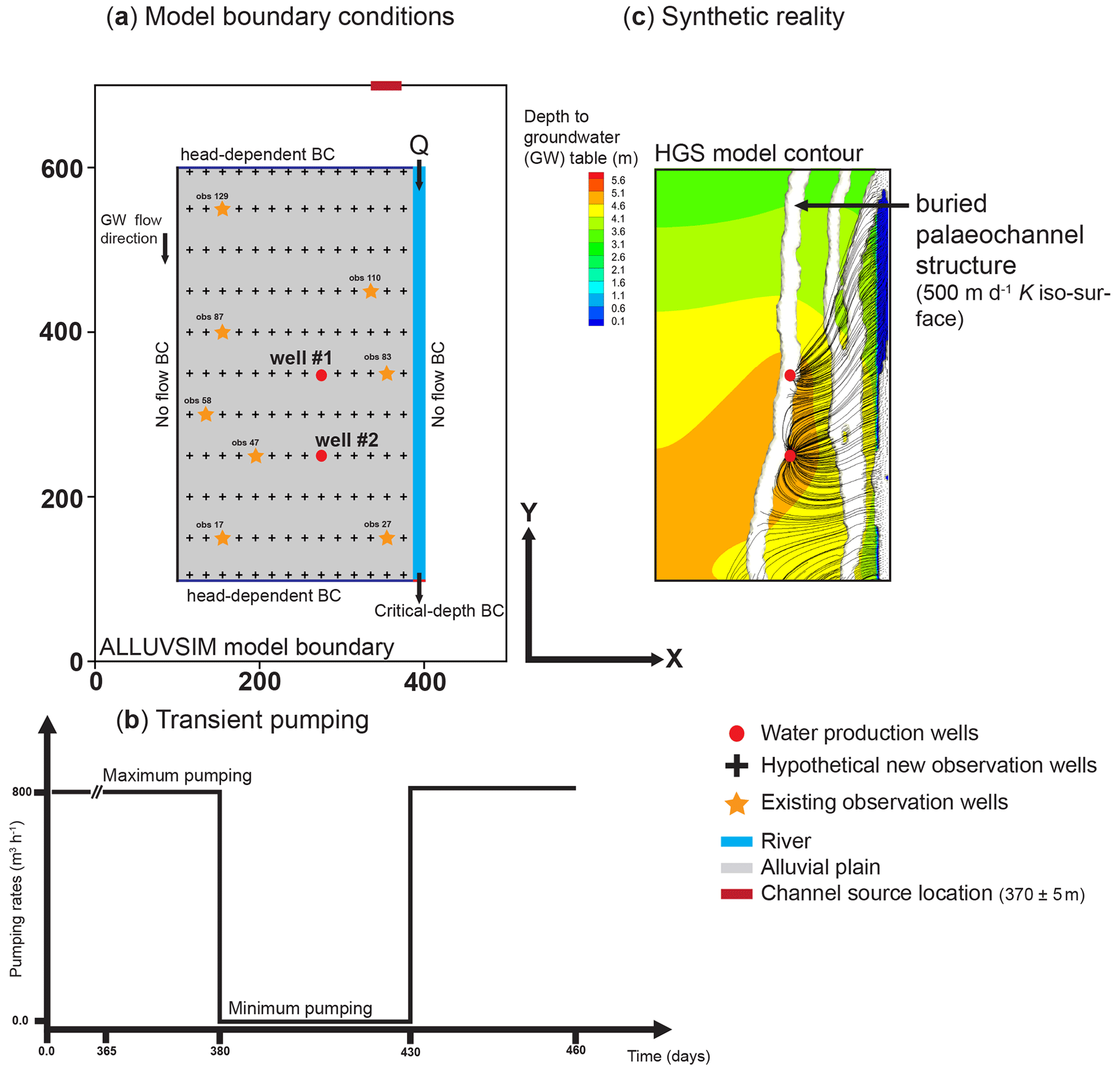
Figure 1 (a) Model boundary conditions and observation points that are discussed herein. (b) Transient pumping rates for the two production wells over a period of 95 d; note that the pumping rate is reduced to zero for a period of 50 d. (c) “Synthetic reality” showing “true” alluvial channels that govern hydraulic properties such as hydraulic conductivity and porosity. Depth to groundwater table under the maximum pumping regime is also shown and so too are the paths of particles (black lines converging towards water production wells) that are used to calculate travel times to water production wells.

In our synthetic example, the objective of our numerical experiments is to mimic real-world modelling as it is undertaken in many alluvial depositional environments with which we are familiar. The numerical model is therefore constructed to predict surface water infiltration along a river and surface water travel times to water production wells with particular emphasis on the shortest of these times. Both of these variables are relevant to the management of an alluvial aquifer used for drinking water supply. The provision of these predictions by a numerical model can, for example, assist water managers in operating a well field in a way that minimizes the potential for bacterial contamination of drinking water (Epting et al., 2018). In this example, we investigate the ability of DSI to associate uncertainties with management-pertinent predictions and to support data acquisition strategies which may further reduce these uncertainties.

3.1 Numerical model

It is essential to consider interactions and feedback mechanisms between the surface and sub-surface when simulating alluvial aquifers that are connected to rivers. Integrated surface and sub-surface hydrologic models (ISSHMs) provide a consistent framework for simulating flow and transport processes for such systems (Schilling et al., 2022; Brunner et al., 2017). An important feature of these models is that they can dynamically simulate feedback between the surface and sub-surface water regimes over a wide range of temporal and spatial scales (Simmons et al., 2020; Paniconi and Putti 2015). The ISSHM modelling platform HydroGeoSphere (HGS) (Aquanty Inc., 2022; Brunner and Simmons 2012; Brunner et al., 2012) is used to perform the numerical simulations documented herein. HGS simulates surface water (SW) and groundwater (GW) flow processes using a globally implicit, finite-difference flow formulation. Simulation of water flow within the surface water domain is based on the two-dimensional diffusion-wave equation, while the three-dimensional, variability-saturated Richards equation is used to simulate sub-surface flow processes.

3.2 Model setup

3.2.1 Geometry

The numerical flow model deployed to explore and document the capabilities of DSI has a spatial extent of 300 × 500 × 30 m in the x, y and z directions (Fig. 1a). An alluvial plain slopes gently towards the river outlet with a slope of 0.003 m m⁻¹ in the y direction. The river itself flows along the eastern boundary of the model domain in a 3 m deep and 15 m wide channel. The numerical grid is discretized using a two-dimensional unstructured triangular mesh with lateral internodal spacing that ranges between 4 m along the river and 7 m under the proximal alluvial plain. The two-dimensional mesh was generated using AlgoMesh (HydroAlgorithmics Pty Ltd, 2022). The model has 14 layers. Layer boundaries are at depths of 0.5, 1.0, 1.5, 2.0, 3.0, 4.0, 5.0, 8.0, 11.0, 14.0, 17.0, 20.0, 23.0 and 26.0 m. The bottom of the model is at a depth of 30 m. The resulting three-dimensional mesh consists of 112 240 nodes and 204 000 elements (or cells).

3.2.2 Boundary conditions

The surface water inflow on the upstream side of the river is conceptualized through a second-type (specified flux) boundary corresponding to a constant flow (Q) of 7200 m³ h⁻¹. The surface water outflow is implemented as a so-called “critical depth boundary”, which allows surface water to leave the overland flow area downstream (Fig. 1a). Meanwhile, an areal infiltration rate of 300 mm yr⁻¹ is imposed over all nodes of the alluvial plain that borders the river. This top boundary condition represents effective rainfall, as evapotranspiration processes are not explicitly simulated by the model. At the northern and southern ends of the groundwater system, a head-dependent (Cauchy-type) boundary condition is deployed to ensure regional groundwater in- and outflow at these upstream and downstream model boundaries, respectively. Lateral model boundaries, as well as the basal model boundary, are impermeable.

Two production wells are represented by nodal flux boundary conditions; each well extracts 400 m³ h⁻¹ from the groundwater system. In each well the pump is placed at an elevation of 85 m (i.e. at a depth of approximately 14 m). As in all ISSHMs, streamflow simulation is explicit. The exchange between the surface and the sub-surface is based on the heads calculated for the two flow domains and a coupling length between them (the so-called dual-node approach). For this example, we use a coupling length of 0.1 m.

The simulation covers a period of 460 d. Over this period, the model runs for 365 d for the initialization of hydraulic conditions. Then, over the next 95 d, extraction rates from the two water production wells are varied to mimic a controlled pumping experiment (Fig. 1b). During this experiment, well field extraction is shut down for 50 d. The pumping rate is then restored to its initial value of 400 m³ h⁻¹ per well, and the simulation continues for another 30 d. This pumping rate reduction experiment introduces significant transience to the groundwater system. The induced transience has the potential to provide a significant amount of information on the hydraulic properties of the system. This setup is loosely based on a real-world experiment that was conducted in the Aeschau plain, Switzerland (Schilling et al., 2017).

The average computational time required for the model to simulate the transient simulation is 10 min; the simulation is not parallelized. HGS employs adaptive time-stepping; however, the maximum time step is limited to a single day in order to ensure numerical stability.

3.2.3 Parameterization

The generation of realistic distributions of sub-surface hydraulic properties in depositional environments that are characterized by distinct, continuous features of complex geometry such as alluvial channels is often implemented using rule-based feature-generation codes. Alternatively, packages which implement multiple-point geostatistics (Remy et al., 2009; Linde et al., 2015) can be employed. Algorithms that underpin the former codes generate structures that can have similar geometric properties to alluvial channels, whereas the latter packages employ stochastic image analysis techniques to reproduce these structures while maintaining hydraulic property connectedness.

Table 1 Model parameters used for the synthetic reality and prior parameter means and uncertainties used for prior ensemble generation.

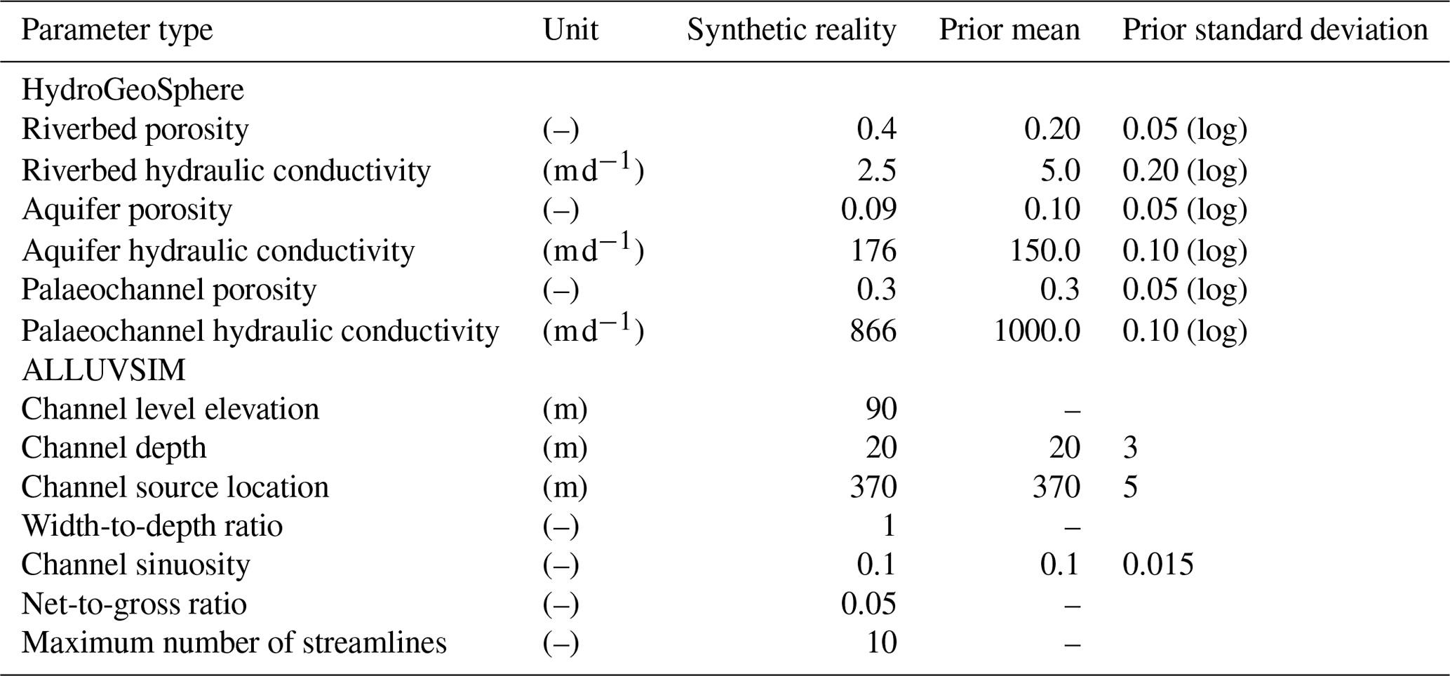
In the present case, we employed the ALLUVSIM alluvial channel simulator (Pyrcz et al., 2009) to generate distributions of the alluvial sub-surface. (Note that the distribution of the alluvial channels does not affect the present location of the river; conceptually they are remnants of historical river channels). The numerical generation of superimposed and intersecting alluvial channels is controlled by geometric (and stochastic) input parameters such as channel depth, width, porosity, starting location and sinuosity (Pyrcz et al., 2009); see Table 1. ALLUVSIM simulations were used to assign sets of alluvial channels to the HGS groundwater flow domain.

For the generation of ALLUVSIM channel sets we adopted a width-to-depth ratio of 1. Furthermore, the depth of channel deposits averages 20 m, this being a considerable portion of the modelled sub-surface. Recall that the depth of the base of the model is 30 m. We do not stack channels at different depths. Therefore, each distribution of the sub-surface contains a small number (up to 10) of alluvial channels, each of which is continuous from the north to the south of the model domain while extending from the surface to a depth that approaches the bottom of the alluvium. As is apparent in Table 1, the mean channel x coordinate (about 370 m from the western edge of the ALLUVSIM model boundary along its northern boundary) is such that channels tend to occupy parts of the sub-surface that are not too far from the course of the present river. Groundwater flow within the near-river part of the model domain is therefore dominated by the presence of these continuous, conductive channels. One of the ALLUVSIM-generated channel distributions (out of a total of 101) was adopted as the “reality” channel distribution. This is displayed in Fig. 1c. The other 100 channel distributions were used to generate realizations of prior hydraulic properties in the HGS groundwater flow domain. These prior realizations are required by the DSI process described above.

Prior realizations of hydraulic properties contain three facies; these facies are channel, non-channel and riverbed deposits. This last facies is present below the current river location and develops in the upper layer of the HGS model to a depth of 50 cm. For each HGS model realization, each of these facies was provided with a spatially uniform set of hydraulic properties (i.e. hydraulic conductivity and porosity). The value of each of these properties was randomly selected from probability distributions that are presented in Table 1. (Intra-facies heterogeneity was purposefully neglected to examine DSI's performance in geological settings where hydraulic properties are categorical, with one category exerting a dominant influence on groundwater flow.) Appendix A depicts a number of HGS model parameter realizations, coloured according to horizontal hydraulic conductivity.

A vertical anisotropy of 4 was assigned to all hydraulic conductivities in all realizations. This is consistent with alluvial depositional systems similar to those that our study attempts to represent (Gianni et al., 2018; Chen 2000; Ghysels et al., 2018).

Parameters that govern unsaturated flow are homogeneous and invariant between realizations. The van Genuchten–Mualem parameters a [m⁻¹] and β [–] were set to 3.48 and 1.75, respectively, these being typical of alluvial gravel (Dann et al., 2009). The residual soil water content was set to 0.095. The Manning's roughness coefficient was set to 1.7 × 10⁻⁶$\mathrm{d}{\mathrm{m}}^{-\mathrm{1}/\mathrm{3}}$.

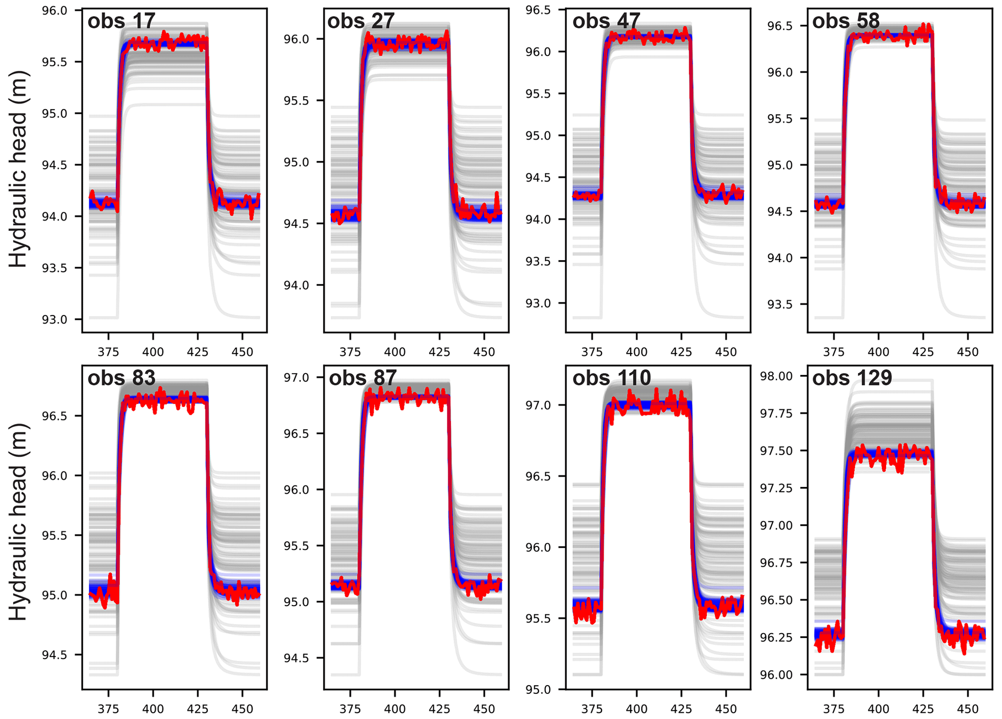
Figure 2 Observations of hydraulic heads (red); these are calculated by the “synthetic reality” of the HGS parameter field. Heads calculated by the remaining realizations are shown in grey. Heads calculated using posterior hydraulic property realizations are shown in blue; there are 70 of these.

3.3 History-matching dataset and model predictions

The dataset used for history matching consists of 95 observations of hydraulic heads in each of the eight observation wells, providing a total of 760 individual observations. These heads were calculated using the HGS “reality parameter field”. A random realization of measurement noise was added to each head measurement. The probability density distribution of synthetic head measurement noise has a mean of 0.0 m and a standard deviation of 0.05 m. Figure 2 shows “reality heads” together with heads calculated at the same locations using the remaining 100 hydraulic property realizations. There is considerable scatter in these plots. This suggests that the information content of these heads concerning sub-surface hydraulic properties is high. Their information content with respect to predictions of interest is pursued using the methodologies discussed above.

The predictions of interest are as follows:

• fast travel times (days) at the first well (well no. 1);

• fast travel times (days) at the second well (well no. 2);

• rate of surface water infiltration into the groundwater system (l s⁻¹) along the entire length of the river.

Travel times are calculated using particles; see Anderson et al. (2015) for details. For each realization of the alluvial architecture and accompanying hydraulic properties, particles are placed along the riverbed at the top of the sub-surface flow domain; see Fig. 1c. Most particles leave the model domain through one of the two extraction wells. The travel time that corresponds to the 5th percentile of the particle breakthrough curve at a particular well under normal operating conditions is deemed to be the “fast travel time” pertaining to that well. Our focus on fast-moving water acknowledges the likelihood of rapid flow processes being driven by preferential flow paths. These same rapid flow processes can threaten water extraction in the event of surface water contamination.

Fast times and surface water infiltration are calculated at t = 365 d. Thus they pertain to maximum well abstraction rates.

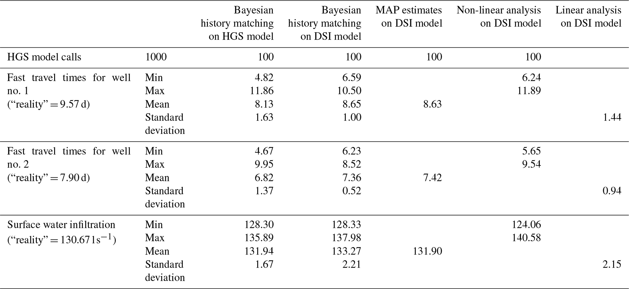
For the synthetic reality, the 5th percentile of travel times is 9.57 and 7.90 d for water production wells no. 1 and no. 2, respectively. Meanwhile, surface water infiltration along the entire river is 130.67 l s⁻¹.

4 Uncertainty quantification

In this section, we document how the posterior (i.e. post-history-matching) uncertainties of the three predictions of interest can be evaluated using four different approaches. One of these requires the adjustment of the parameters of the HGS model. The other three approaches require the adjustment of parameters of a surrogate model that is built to implement DSI-based predictive uncertainty evaluation in ways that are discussed in Sect. 2. In all cases parameter adjustment minimizes a least squares objective function that serves as a measure of model-to-measurement misfit. This objective function is calculated as the sum of weighted squared differences between observed and modelled heads in the eight observation wells discussed above. Weights are uniform to reflect the temporal uniformity of measurement noise; each has a value that is equal to the square of the standard deviation of this noise. The expected value of the history-matched objective function is therefore expected to be somewhat greater than 760, this being the number of observations which comprise the calibration dataset. The “somewhat greater” is an outcome of the fact that the number of “effective parameters” is unknown prior to solving an ill-posed inverse problem; see Doherty (2015) for details.

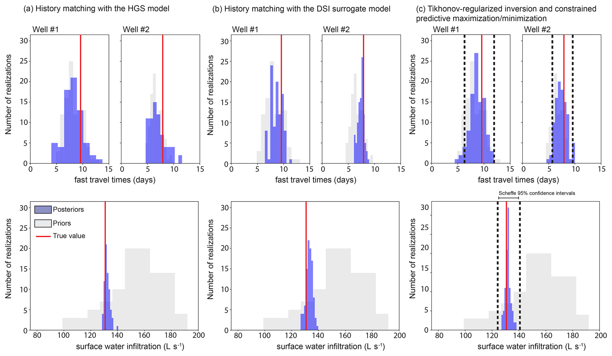
Figure 3 Posterior distributions of model predictions of fast travel times (days) and surface water infiltration (L s⁻¹) with (a) the application of IES (after three iterations) to the HydroGeoSphere (HGS) model ensemble, (b) the application of IES (after six iterations) to the surrogate model ensemble, and (c) the application of Eq. (21) (linear analysis) and Eq. (20) (non-linear analysis) with the MAP estimate of the DSI surrogate model. The dashed lines in (c) represent values for Scheffe 95 % confidence intervals.

4.1 Bayesian history matching

4.1.1 History matching with the HGS model

Prior to using DSI for the exploration of predictive uncertainty, we adjust HGS model parameters using the PESTPP-IES ensemble smoother. History-match-constrained parameter fields were then used to make the predictions of interest. The variability in these predictions between these posterior parameter fields is a measure of their posterior uncertainties.

The ensemble smoothing process begins with samples of the prior parameter probability distribution. In the present case, we used the 100 parameter fields that were obtained in the manner discussed above. These parameter fields are iteratively adjusted until model outputs fit field measurements. The HGS model has 204 000 adjustable elements, these being hydraulic conductivities and porosities ascribed to individual model cells. As is common practice when using parameter ensembles for history matching, each of these is considered a separate parameter when undertaking PESTPP-IES-based parameter adjustment.

Piecewise spatial uniformity of the initial parameter fields is lost during the ensemble parameter adjustment process as each parameter is subject to individual adjustment while maintaining a high level of spatial correlation with neighbouring parameters that is inherited from the initial realizations. See Chen and Oliver (2013) for mathematical details of the parameter adjustment process.

The objective function associated with all ensemble realizations was significantly reduced after three iterations of the IES parameter adjustment process. Objective function values ranged between 1075 and 16 098, except for 30 realizations which suffered excessively slow HGS model solution convergence and were therefore abandoned. Note that each iteration of the IES parameter adjustment process requires as many model runs – in this case HGS model runs – as there are realizations that comprise the ensemble. Figure 2 shows that model-calculated heads at the observation wells are indeed close to “measured” heads. The 70 realizations which remained after three IES iterations were used to make the predictions that are described above. The results are plotted in Fig. 3a.

It can be seen from Fig. 3a that the uncertainty of predicted surface water infiltration is significantly reduced by PESTPP-IES-based history matching of the HGS model. It can therefore be concluded that the information content of hydraulic heads with respect to this specific prediction is high. In contrast, the uncertainties of first arrival travel time predictions are not significantly reduced; see Fig. 3a. The information content of head responses to altered pumping rates with respect to these predictions is therefore lower than it is for surface water infiltration.

An interesting feature of Fig. 3a is that some posterior parameter fields have fast travel times that exceed those calculated using prior parameter fields. This can be explained by the fact that some posterior parameter fields have lost some of the connectivity exhibited by the prior parameter fields. (see Appendix B). This is an outcome of the PESTPP-IES parameter adjustment process which is only truly Bayesian where prior parameter distributions are Gaussian on a cell-by-cell basis (if cell-by-cell parameterization is employed). However, the prior realizations that compose the initial ensemble from which the IES inversion process has started are not multi-Gaussian (see Appendix A). Neither the theory on which IES is based nor numerical implementation of that theory in its history-matching algorithm can guarantee the maintenance of long-distance hydraulic property connectedness which cannot be characterized by a multi-Gaussian distribution. Indeed, history-match-constrained adjustment of connected and categorical parameter fields is still an area of active research (Khambhammettu et al., 2020). Note that while uncertainty analysis methods such as rejection sampling or Markov chain Monte Carlo approaches do not require a Gaussian prior or a Gaussian likelihood function, these methods are impractical in contexts where the number of parameters is high and model run times are long, which is the case for the many hydrogeological applications and for the example used in this paper.

4.1.2 History matching with the DSI surrogate model

The same 100 samples of the prior parameter probability distribution that were used to start the PESTPP-IES data assimilation process were then used to construct a DSI surrogate model using the methodology described in Sect. 2. Recall that this surrogate model is based on an empirical covariance matrix that relates history-matched model outputs to predictive model outputs. A singular value energy level of 0.999 was used in the construction of this surrogate model. This results in the use of 87 singular values (and corresponding eigencomponents) of this matrix and hence an 87-dimensional x vector; see Eq. (6). Note that the only HGS model runs that were required to construct and history-match the DSI surrogate model were those that were based on the 100 prior hydraulic property field realizations discussed above. No further runs of the HGS model were required to carry out any of the procedures described below.

Sampling of the posterior distribution of surrogate model parameters (i.e. elements of the x vector) was implemented using the PESTPP-IES ensemble smoother. However, in contrast to the previous use of PESTPP-IES, its use with the DSI surrogate model incurs a trivial numerical burden because of the extremely fast execution speed of this model. An ensemble comprising 100 realizations of the prior probability distribution of surrogate model parameters was adjusted. After six iterations of this process, all realizations yielded good model-to-measurement fits, with objective function values ranging between 814 and 830. Prior and posterior prediction histograms are shown in Fig. 3b.

The posterior prediction probability distributions for surface water infiltration calculated by HGS parameter adjustment on the one hand and by DSI surrogate model parameter adjustment on the other hand are very similar. The same cannot be said for fast travel times. The posterior uncertainty of this prediction is lower after DSI surrogate model parameter adjustment than after HGS model parameter adjustment. This suggests that estimation of DSI surrogate model parameters does not suffer the same degradation in uncertainty evaluation performance as that which is incurred by PESTPP-IES-based adjustment of HGS parameters which tend to lose their continuity as the history-matching process progresses. In contrast, parameters of the DSI surrogate model are not required to maintain any spatial patterns or relationships; they must simply represent observation-to-prediction relationships that are embodied in 100 HGS model outputs that were all calculated using continuous hydraulic property parameter fields.

4.2 Tikhonov-regularized inversion and constrained predictive maximization and minimization

The DSI surrogate model was calibrated using Tikhonov regularization; see Eq. (14). The MAP estimates of x obtained in this way were used to calculate MAP values of predictions. These are listed in Appendix C.

Following calibration of the DSI surrogate model, Eq. (21) was used to calculate the prior and posterior standard deviations of the uncertainties of the three predictions of interest based on an assumption of surrogate model linearity. Sensitivities of model outputs that correspond to members of the calibration dataset and that correspond to model predictions were calculated using finite difference perturbations from calibrated surrogate model parameter values. Linear-calculated standard deviations were then used to plot the probability density distributions for the three predictions so that they could be compared with ensemble-calculated standard deviations (Fig. 3c).

Next, posterior uncertainties of the three predictions of interest were calculated using the constrained maximization and minimization procedure that is described by Eq. (20). The objective function constraint provided to this equation was that which enables the calculation of Scheffe 95 % confidence intervals (see Vecchia and Cooley, 1987). The values obtained through this process agree reasonably well with maximum and minimum predictions obtained through Bayesian history matching of the DSI surrogate model (Fig. 3c).

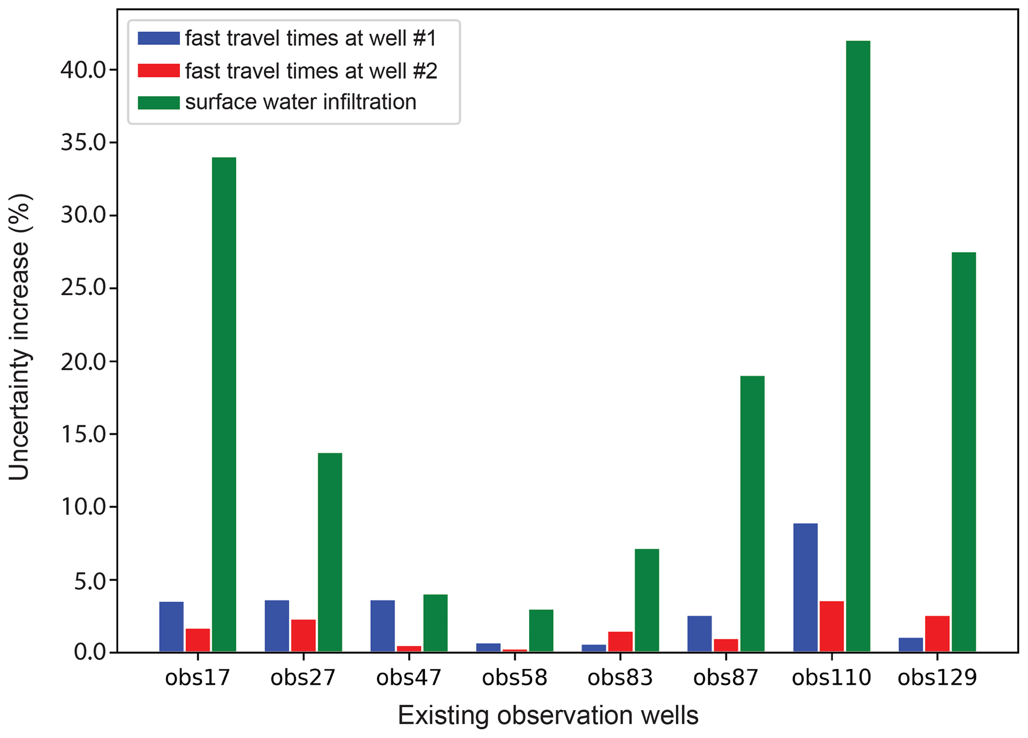
Figure 4 Percent increase in the standard deviation of posterior uncertainty of each of the three predictions discussed herein when one existing observation well is removed from the current observation dataset.

Differences between evaluated predictive uncertainties that appear in Fig. 3 (statistics are available in Appendix C) are generally small; however, some are large enough to warrant discussion. Differences between linear and non-linear uncertainty estimates can be at least partly attributed to approximations that the calculation of these estimates requires. Linear estimation of posterior predictive uncertainty not only requires an assumption of linearity of the DSI model, but it also assumes Gaussianality of the prior probability distributions of DSI model parameters (i.e. elements of the x vector of Eq. 6). Meanwhile, non-linear analysis, involving adjustment of HGS model parameters by PESTPP-IES, is prone to sampling errors incurred through the use of only 100 realizations; it is also affected by problems that beset PESTPP-IES in maintaining continuity of hydraulic properties (see above). Another factor that may degrade the accuracy of posterior uncertainties calculated using the HGS model is failure of model outputs based on some parameter realizations to fit measured heads to within limits that are set by the statistical properties of measurement noise. Nevertheless, in spite of these approximations, it is pleasing to note that the ratio of prior to posterior uncertainty is reasonably consistent between all linear and non-linear estimates of posterior predictive uncertainty. This increases confidence in the data worth analysis which is the subject of the next section.

5 Data worth

Quantifying the effectiveness and efficiency of existing and planned data acquisition and monitoring strategies can (and often should) be an important outcome of decision-support groundwater modelling. This is because the quantification of uncertainty brings with it an ancillary benefit, this being the quantification of the extent to which existing or anticipated data acquisition can reduce the uncertainties of one or more decision-critical model predictions. The worth of data increases in proportion to their ability to achieve this outcome.

5.1 Worth of existing data

The worth of data and subsets thereof that already comprise the calibration dataset can be evaluated according to two different metrics. The worth of subsets of existing data can be assessed by evaluating the extent to which the posterior standard deviations of decision-critical model predictions are increased by their omission from this dataset. The worth of these subsets can also be assessed by evaluating the extent to which the prior standard deviation of these predictions is reduced by including a particular subset as the only member of the history-matching dataset. In the present section, we evaluate the worth of existing data according to the first of these metrics only. This is implemented using linear analysis based on Eq. (21). It is worth noting that, because the surrogate model runs so fast, the ensemble smoother could also have been used to sample the posterior distribution of our predictions with the omission of certain subsets of the history-matching dataset.

Using Eq. (21), data are notionally omitted in a calibration dataset simply by setting their associated weights to values of zero. This was done for each of the observation wells that are featured in Fig. 1a. The outcomes of this analysis are presented in Fig. 4.

An inspection of Fig. 4 reveals that members of the existing observation network are more informative of predictive flux than they are of fast travel times. Furthermore, the cost of omitting OBS110 from the existing observation network appears to be greater than that of omitting any other observation well from the network. This implies a certain degree of uniqueness of information that is forthcoming from this well. This is not surprising as OBS110 is located upstream and closer to sources of surface water infiltration than most of the other observation wells. It is therefore close to the path of much of the water that flows from the river to production wells.

Of particular interest is the high information content of OBS17 data with respect to the prediction of induced infiltration. This is attributable to the fact that prior realizations of hydraulic properties display spatial uniformity within each stratigraphic unit (that is channels, riverbed and other alluvium). Therefore, while pumping-induced surface water infiltration is sensitive to the structure and disposition of palaeochannels which convey water from the river to production wells, it is also sensitive to aquifer properties that can control inflow/outflow of water to/from the northern and southern boundaries of the model domain. The difference in head between OBS17 and the southern head-dependent boundary is informative of these properties. The importance of these head measurements would be reduced if stratigraphic unit properties were internally heterogeneous.

5.2 Worth of a new observation point

Equation (21) can be readily turned to the evaluation of the issue of whether it is worth supplementing the existing observation network of eight observation wells with a new observation well. In our study, contenders for the new observation point are each of the 146 sites that are represented by black crosses in Fig. 1a. We establish the worth of including a new point in the monitoring network by including heads at that point in an expanded history-matching dataset, thereby assuming that observations from this well were available during the calibration period that has formed the basis for all investigations that have been discussed so far. The reduction in the uncertainty standard deviation of management-pertinent predictions that is accrued through the expansion of the history-matching dataset in this way is a measure of the worth of the hypothesized new data. Recall from the discussion in Sect. 2 of this paper that Eq. (21) does not require the values of observation to assess their worth. It requires only the sensitivities of corresponding model outputs to model parameters.

We base our exploration of data worth on a DSI surrogate model. However, HGS model outputs on which this model is based must be extended to include those at the candidate observation wells. This enables the construction of an expanded covariance matrix that links model outputs at these sites to predictions of interest. In our case, these were available from archived output files of the 100 HGS model runs which form the basis for results that are reported in previous sections of this paper. In other cases, another suite of large model runs may be required for the construction of a new surrogate model. Note, however, that once these model runs have been completed, all further analyses can be conducted using the DSI surrogate model.

To verify this linear approach to data worth assessment, reductions in predictive uncertainty that would result from updating the calibration dataset to include heads from each of the 146 potential observation wells that are shown in Fig. 1a were calculated using an alternative (and much more laborious) non-linear approach.

For each of the 100 prior realizations of HGS parameter fields, heads were calculated at each of the 146 trial observation points. For each of these observation points and for each of these parameter realizations, a new DSI model was constructed using the methodology discussed above. The history-matching dataset for each of these models included the existing dataset (comprised of eight observation wells) and the expanded dataset that is pertinent to that well and that particular realization of the prior HGS parameter field. Predictions were the same for each DSI surrogate model (i.e. fast travel times to the production wells and surface water infiltration). Each of these 14 600 DSI surrogate models was then history-matched against its respective history-matching dataset to obtain the posterior uncertainties of our predictions of interest. This was done using the PESTPP-IES ensemble smoother. For each trial observation well, the “total” posterior uncertainty of a prediction of interest was calculated by accumulating prediction realizations over all 100 DSI surrogate models that pertained to each expanded observation well. These were compared with the posterior uncertainties calculated using the original DSI surrogate model that was based on a history-matching dataset that did not include the new well.

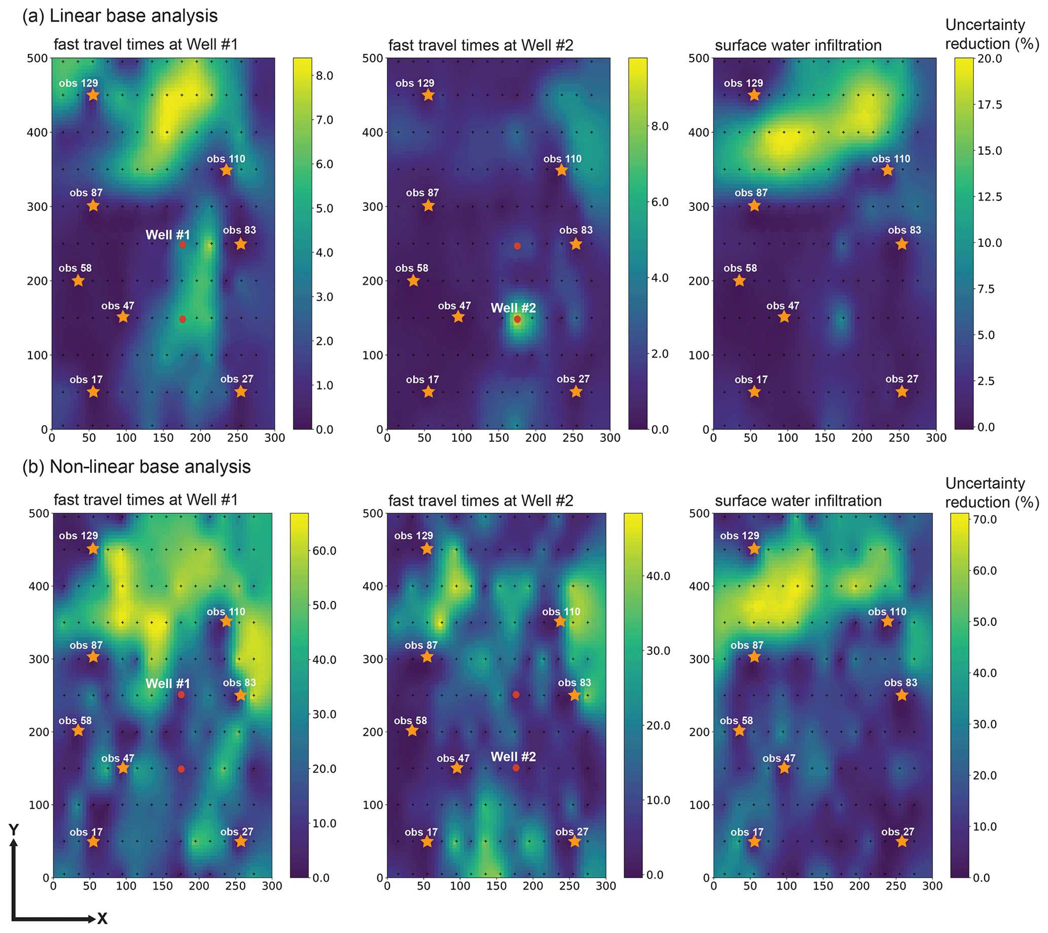
Figure 5 Percent decrease in posterior uncertainty of each of the three predictions accrued through supplementing the existing calibration dataset with head measurements gathered in an extra well following (a) linear analysis and (b) non-linear analysis.

For both approaches, the percent reduction in the standard deviations of the uncertainties of our predictions was calculated for each of the 154 observation wells. These were then interpolated over the model grid for presentation purposes; see Fig. 5.

Areas of high and low worth of installation of a new observation well are broadly similar between the upper and lower sets of maps that comprise Fig. 5, especially for the surface water infiltration prediction.

It is clear from Fig. 5 that the collection of new hydraulic head data in the northern part of the model has the potential to reduce the uncertainty associated with predictions of surface water infiltration. This also applies to fast travel times to the northern extraction well and to a lesser extent for fast travel times to the southern extraction well. The non-linear analysis also suggests that the acquisition of head data in the river corridor between the existing OBS110 and OBS83 observation wells may yield reductions in uncertainties of fast travel time predictions for both water production wells. To a lesser extent (especially for the southern production well), this is also established through linear analysis. This makes sense, as this zone is crossed by most of the particles that arrive at the production wells.

Both methods for data worth analysis that are described above are based on approximations. Non-linear analysis suffers from the limited number of realizations on which it is based. Obviously, linear analysis suffers from an assumption of DSI surrogate model linearity. Nevertheless, despite these approximations, the two approaches yield results that are in broad agreement with each other. Furthermore, they are both readily deployable in real-world contexts where hydraulic property distributions and processes are complex; this applies especially to DSI-based linear analysis.

6 Discussion and conclusions

The purpose of this paper is to document and demonstrate the use of data space inversion (DSI) as a means of quantifying and reducing the posterior uncertainties of predictions made by complex models with complex parameter fields. Both model attributes make the application of traditional uncertainty analysis difficult. Model complexity increases model run time; it can also increase the propensity of a model to exhibit unstable numerical behaviour when endowed with a stochastic parameter field. The complexity of parameterization, especially when it involves the use of continuous, connected hydraulic properties (as illustrated in our example), can violate the assumptions upon which these properties are adjusted in order for model outputs to respect measurements of system behaviour.

Data space inversion addresses the first of these challenges by replacing a numerical model with a fast-running DSI surrogate model. This surrogate model is tuned to the decision-support role for which the original, complex model was built. This is because the DSI surrogate model is designed to replicate the ability of a numerical model to simulate past measurements of system behaviour and to make predictions of future system behaviour that are of interest to management. Both of these complex model outputs can be calculated using parameter fields of arbitrary complexity that represent aspects of the sub-surface that are critical to past and future groundwater behaviour. In many cases, these will include structural or alluvial features that can rapidly transport water and dissolved contaminants to points of environmental impact.

Realizations that compose the initial ensemble from which model outputs are calculated do not have to be multi-Gaussian. The multi-Gaussian assumption used to link measurements of past system behaviour to predictions of future system behaviour is independent of any assumptions about the prior realizations. Because a direct link is made between measurements and predictions (thereby bypassing parameters), an assumption of multi-Gaussianality is likely to have a weaker effect on the results of the predictive uncertainty analysis process than highly parameterized methods that rely implicitly or explicitly on parameter adjustment (such as linear Bayesian methods, randomized maximum likelihood methods and iterative ensemble smoother methods). Thus, prior realizations used to start the DSI process can accommodate both aleatory and epistemic uncertainties. Uncertainties in prior parameter distributions can also be readily accommodated.

A strength of the DSI methodology is that it does not require the adjustment of hydraulic property fields for model outputs to replicate the past so that they can be used as a basis for posterior sampling of future groundwater behaviour. Instead, the parameters and predictions of a DSI surrogate model (rather than the original model) are subjected to adjustment and posterior sampling. The nature of these surrogate model parameters is such that they embody the parameterization complexity of the original model without replicating it. Instead, they are formulated to reproduce the effects of that complexity on the model outputs used for both history matching and system management. Thus, the complex nuances of system hydraulic properties are implicitly taken into account as predictions of future system behaviour are conditioned by measurements of past system behaviour.

This paper demonstrates that the use of a DSI surrogate model can extend beyond that of sampling the posterior probability distribution of one or several predictions of interest. Like a conventional numerical model, it can be used for the rapid assessment of the worth of existing or new data. The simplest (and most rapid) form of data worth analysis relies on an assumed linear relationship between surrogate model parameters and surrogate model outputs. There may be many circumstances where this linearity assumption is more applicable than that of a linear relationship between conventional model parameters and conventional model outputs, as the latter relationships are bypassed in the definition and construction of the DSI surrogate model and its parameters. The DSI-based evaluation of data worth may therefore be more reliable than the evaluation of data worth using a complex model. In fact, if a complex model has many parameters (as it should), and its run times are high (as they often are), the calculation of sensitivities that are required for linear analysis may not be possible. Meanwhile, by construction, the parameters of a DSI surrogate model can take the complex dispositions and connectivity relationships of real-world hydraulic properties into account.

This paper also demonstrates more complex uses to which a DSI surrogate model can be put. Tikhonov-regularized inversion and constrained, non-linear prediction optimization are demonstrated in Sect. 4. Section 5 demonstrates how more complex assessments of data worth can be made than that which relies on an assumption of surrogate model linearity. While the numerical costs associated with these assessments are high, they are far from prohibitive.

However, together with strength comes weakness. It is acknowledged that while the DSI methodology enables rapid and effective posterior uncertainty analysis in contexts that may otherwise render such analyses approximate at best and impossible at worst, a modeller is entitled to feel a sense of frustration at not being able to “see for themself” the parameter fields that give rise to predictive extremes. Not only may an understanding of these fields add to a modeller's understanding of a system, but it may accomplish the same thing for decision-makers and stakeholders as well.

Appendix A: Prior realizations of alluvial structural features

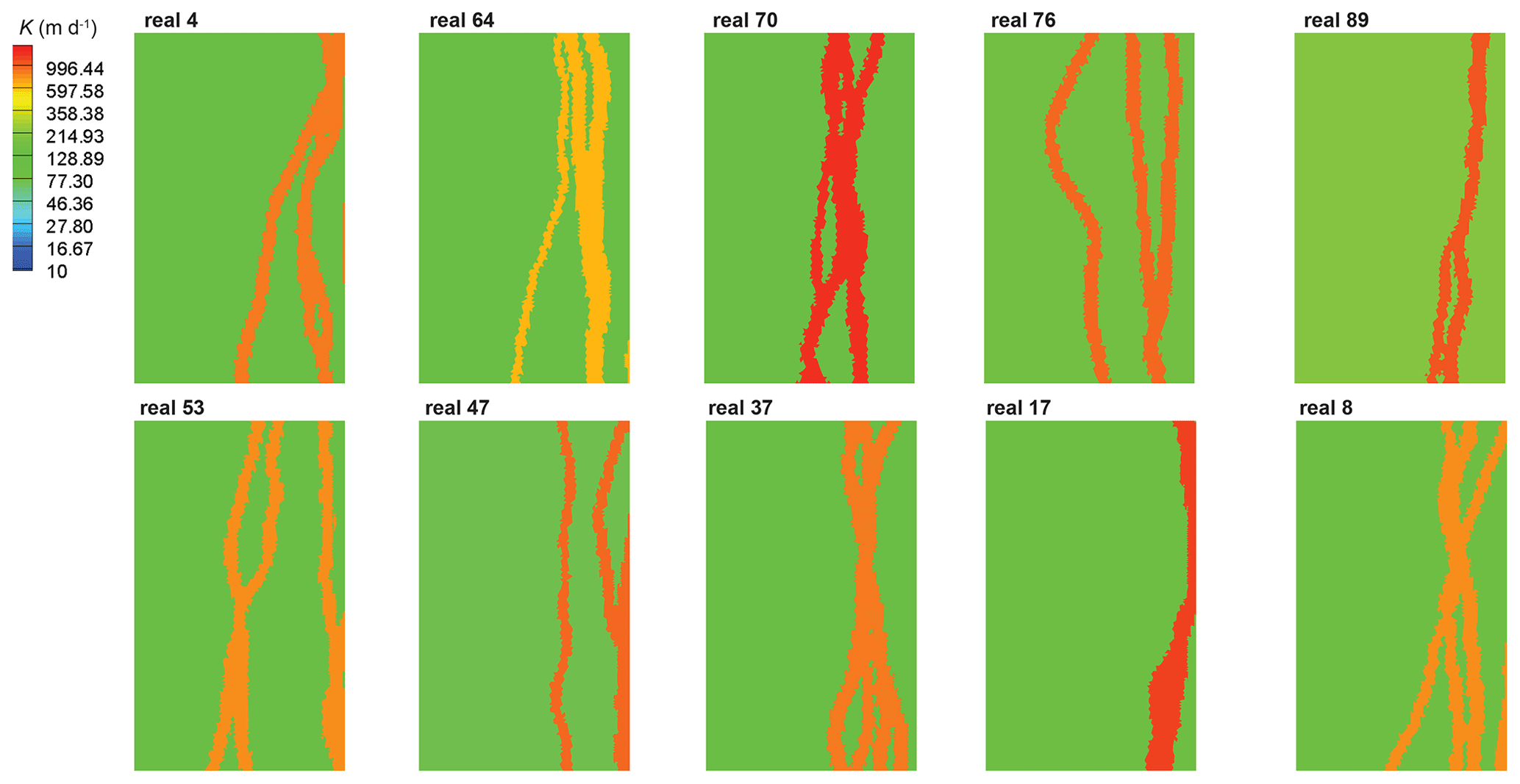
Figure A1 Prior realizations of alluvial structural features generated from ALLUVSIM and mapped into the HGS model for hydraulic conductivity (K) parameterization.

Appendix B: Posterior estimates of hydraulic conductivity fields

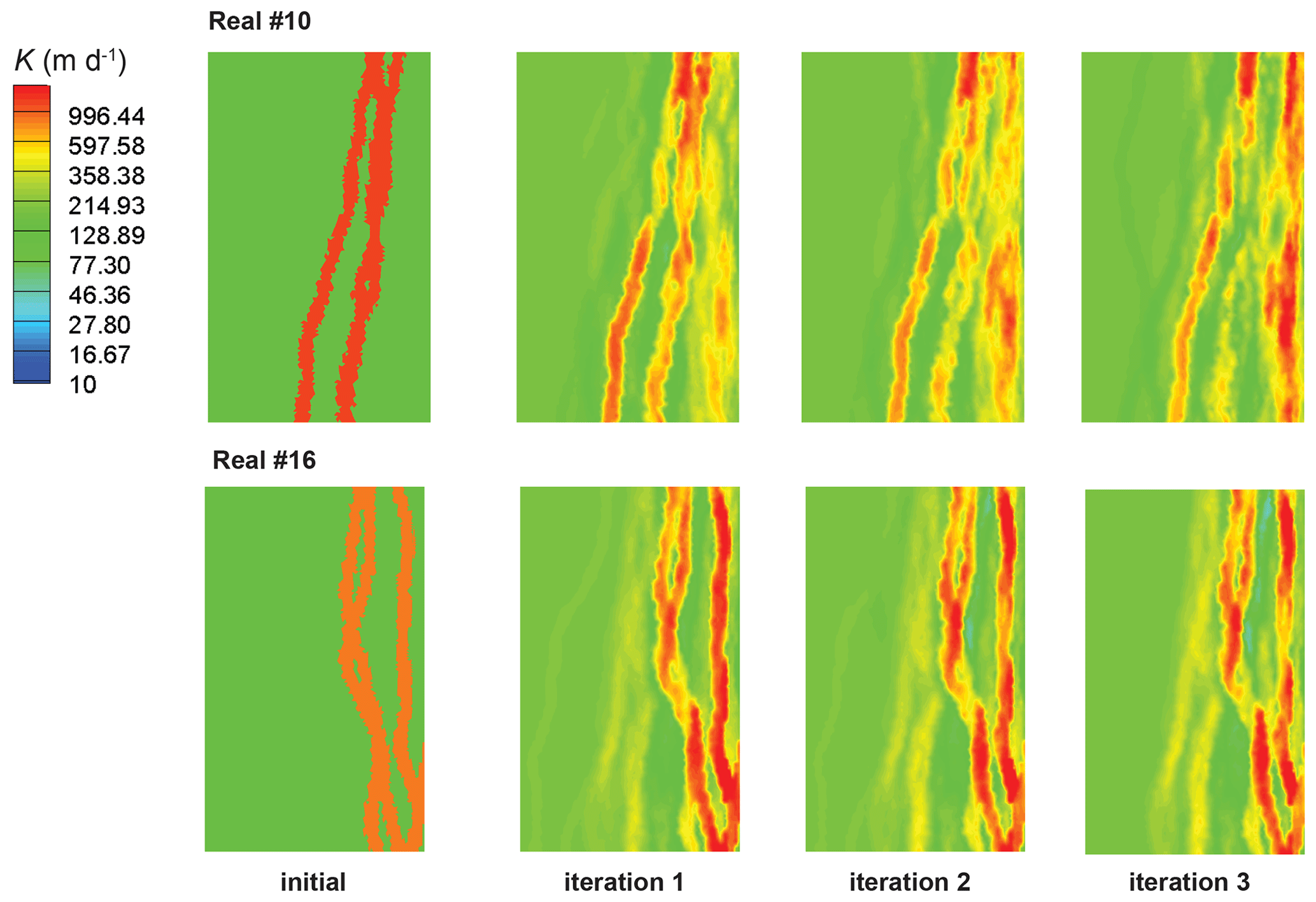
Figure B1 Posterior estimates (for realization numbers 10 and 16) of hydraulic conductivity (K) after applying the iterative ensemble smoother over three iterations by adjusting the HGS model parameters with the existing dataset.

Appendix C: Posterior uncertainty statistics

Table C1 Posterior uncertainty statistics of distributions shown in Fig. 3.