Evaluating precipitation distributions at regional scales: a benchmarking framework and application to CMIP5 and 6 models

As the resolution of global Earth system models increases, regional-scale evaluations are becoming ever more important. This study presents a framework for quantifying precipitation distributions at regional scales and applies it to evaluate Coupled Model Intercomparison Project (CMIP) 5 and 6 models. We employ the Intergovernmental Panel on Climate Change (IPCC) sixth assessment report (AR6) climate reference regions over land and propose refinements to the oceanic regions based on the homogeneity of precipitation distribution characteristics. The homogeneous regions are identified as heavy-, moderate-, and light-precipitating areas by K-means clustering of Integrated Multi-satellitE Retrievals for Global Precipitation Measurement (GPM) version 6 final run product (IMERG) precipitation frequency and amount distributions. With the global domain partitioned into 62 regions, including 46 land and 16 ocean regions, we apply 10 established precipitation distribution metrics. The collection includes metrics focused on the maximum peak, lower 10th percentile, and upper 90th percentile in precipitation amount and frequency distributions; the similarity between observed and modeled frequency distributions; an unevenness measure based on cumulative amount; average total intensity on all days with precipitation; and number of precipitating days each year. We apply our framework to 25 CMIP5 and 41 CMIP6 models, as well as six observation-based products of daily precipitation. Our results indicate that many CMIP5 and 6 models substantially overestimate the observed light-precipitation amount and frequency, as well as the number of precipitating days, especially over midlatitude regions outside of some land regions in the Americas and Eurasia. Improvement from CMIP5 to 6 is shown in some regions, especially in midlatitude regions, but it is not evident globally, and over the tropics most metrics point toward degradation.

1 Introduction

Precipitation is a fundamental characteristic of the Earth's hydrological cycle and one that can have large impacts on human activity. The impact of precipitation depends on its intensity and frequency characteristics (e.g., Trenberth et al., 2003; Sun et al., 2006; Trenberth and Zhang, 2018). Even with the same amount of precipitation, more intense and less frequent rainfall is more likely to lead to extreme precipitation events such as floods and drought compared to less intense and more frequent rainfall. While mean precipitation has improved in Earth system models, the precipitation distributions continue to have biases (e.g., Dai, 2006; Fiedler et al., 2020), which limits the utility of these simulations, especially at the level of accuracy that is increasingly demanded in order to anticipate and adapt to changes in precipitation due to global warming.

Multi-model intercomparison with a well-established diagnosis framework facilitates identifying common model biases and sometimes yields insights into how to improve models. The Coupled Model Intercomparison Project (CMIP; Meehl et al., 2000, 2005, 2007; Taylor et al., 2012; Eyring et al., 2016) is a well-established experimental protocol to intercompare state-of-the-art Earth system models, and the number of models and realizations participating in CMIP has been growing through several phases from 1 (Meehl et al., 2000) to 6 (Eyring et al., 2016). Given the increasing number of models, developed at higher resolution and with increased complexity, modelers and analysts could benefit from capabilities that help synthesize the consistency between observed and simulated precipitation. As discussed in previous studies (e.g., Abramowitz, 2012), our reference to model benchmarking implies model evaluation with community-established reference datasets, performance tests (metrics), variables, and spatial and temporal resolutions. The U.S. Department of Energy (DOE) envisioned a framework for both baseline and exploratory precipitation benchmarks (U.S. DOE. 2020) as summarized by Pendergrass et al. (2020). While the exploratory benchmarks focus on process-oriented and phenomena-based metrics at a variety of spatiotemporal scales (Leung et al., 2022), the baseline benchmarks target well-established measures such as mean state, the seasonal and diurnal cycles, variability across timescales, intensity and frequency distributions, extremes, and drought (e.g., Gleckler et al., 2008; Covey et al., 2016; Wehner et al., 2020; Ahn et al., 2022). The current study builds on the baseline benchmarks by proposing a framework for benchmarking simulated precipitation distributions against multiple observations using well-established metrics and reference regions. To ensure consistent application of this framework, the metrics used herein are implemented and made available as part of the widely used Program for Climate Model Diagnosis and Intercomparison (PCMDI) metrics package.

Diagnosing precipitation distributions and formulating metrics that extract critical information from precipitation distributions have been addressed in many previous studies. Pendergrass and Deser (2017) proposed several precipitation distribution metrics based on frequency and amount distribution curves. The precipitation frequency distribution quantifies how often rain occurs at different rain rates, whereas the precipitation amount distribution quantifies how much rain falls at different rain rates. Based on the distribution curves, Pendergrass and Deser (2017) extracted rain frequency peak and amount peak where the maximum non-zero rain frequency and amount occur, respectively. Pendergrass and Knutti (2018) introduced a metric that measures the unevenness of daily precipitation based on the cumulative amount curve. Their unevenness metric is defined as the number of wettest days that constitute half of the annual precipitation. In the median of station observations equatorward of 50^∘ latitude, half of the annual precipitation falls in only about the heaviest 12 d, and generally models underestimate the observed unevenness (Pendergrass and Knutti, 2018). In addition, several metrics have been developed to distill important precipitation characteristics, such as the fraction of precipitating days and a simple daily intensity index (SDII; Zhang et al., 2011). In this study we implement all these well-established metrics and several other complementary metrics into our framework.

Many studies have analyzed the precipitation distributions over large domains (e.g., Dai, 2006; Pendergrass and Hartmann, 2014; Ma et al., 2022). Often, these domains comprise both heavily precipitating and dry regions. Given that the emphasis on regional-scale analysis continues to grow as models' horizontal resolution increases, the interpretation of domain-averaged distributions could be simplified by defining regions that are not overly complex or heterogeneous in terms of their precipitation distribution characteristics. Iturbide et al. (2020) have identified climate reference regions that have been adopted in the sixth assessment report (AR6) of the Intergovernmental Panel on Climate Change (IPCC). Our framework is based on these IPCC AR6 reference regions for the objective examination of precipitation distributions over land. Over the ocean we have revised some of the regions of Iturbide et al. (2020) to better isolate homogeneous precipitation distribution characteristics.

In this study, we propose modified IPCC AR6 reference regions and a framework for regional-scale quantification of simulated precipitation distributions, which is implemented into the PCMDI metrics package to enable researchers to readily use the metric collection in a common framework. The remainder of the paper is organized as follows: Sects. 2 and 3 describe the data and analysis methods. Section 4 presents results including the application and modification of IPCC AR6 climate reference regions, evaluation of CMIP5 and 6 models with multiple observations, and their improvement across generations. Sections 5 and 6 discuss and summarize the main accomplishments and findings from this study.

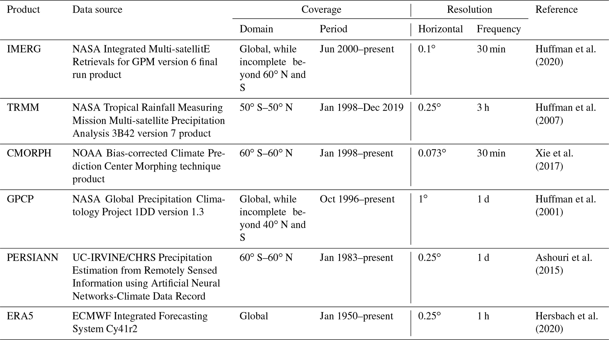
Table 1 Satellite-based and reanalysis precipitation products used in this study.

2 Data

2.1 Observational data

For reference data, we use six global daily precipitation products first made available as part of the Frequent Rainfall Observations on GridS (FROGS) database (Roca et al., 2019) and then further aligned with CMIP output via the data specifications of the Observations for Model Intercomparison Project (Obs4MIPs; Waliser et al., 2020). These include five satellite-based products and a recent atmospheric reanalysis product. The satellite-based precipitation products include the Integrated Multi-satellitE Retrievals for Global Precipitation Measurement (GPM) version 6 final run product (Huffman et al., 2020; hereafter IMERG), the Tropical Rainfall Measuring Mission Multi-satellite Precipitation Analysis 3B42 version 7 product (Huffman et al., 2007; hereafter TRMM), the bias-corrected Climate Prediction Center Morphing technique product (Xie et al., 2017; hereafter CMORPH), the Global Precipitation Climatology Project 1DD version 1.3 (Huffman et al., 2001; hereafter GPCP), and Precipitation Estimation from Remotely Sensed Information using Artificial Neural Networks (Ashouri et al., 2015; hereafter PERSIANN). The reanalysis product included for context is the European Centre for Medium-Range Weather Forecasts's (ECMWF) fifth generation of atmospheric reanalysis (Hersbach et al., 2020; hereafter ERA5). Table 1 summarizes the observational datasets with the data source, coverage of domain and period, resolution of horizontal space and time frequency, and references. We use the data periods available via FROGS and Obs4MIPs as follows: 2001–2020 for IMERG, 1998–2018 for TRMM, 1998–2012 for CMORPH, 1997–2020 for GPCP, 1984–2018 for PERSIANN, and 1979–2018 for ERA5.

Table 2 CMIP5 and CMIP6 models used in this study and their horizontal resolution. The number in parentheses indicates the number of realizations used for each model. Note that the horizontal resolution information is obtained from the number of grids, and it may vary slightly if the grid interval is not linear.

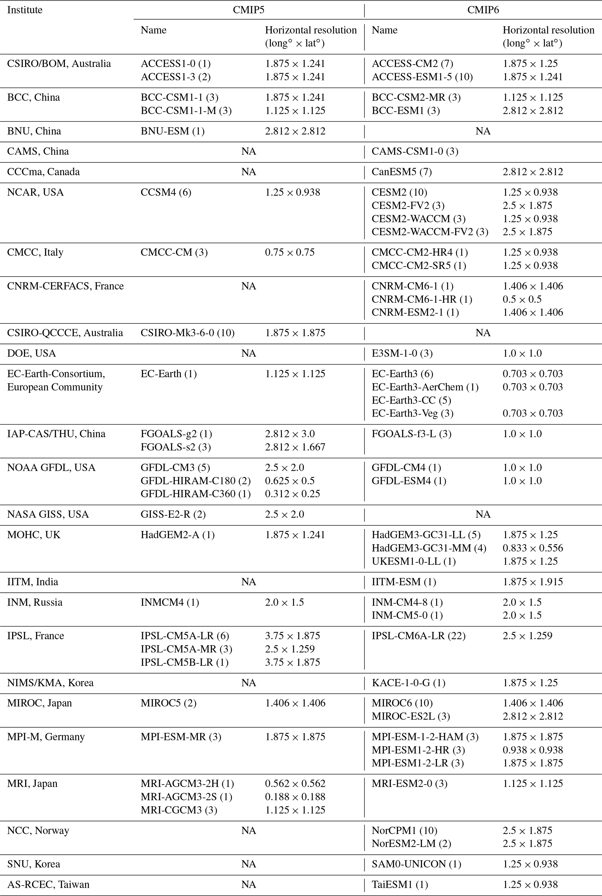
NA: not available

2.2 CMIP model simulations

We analyze daily precipitation from all realizations of Atmospheric Model Intercomparison Project (AMIP) simulations available from CMIP5 (Taylor et al., 2012) and CMIP6 (Eyring et al., 2016). We have chosen to concentrate our analysis on AMIP simulations rather than the coupled historical simulations because the simulated precipitation in the latter is strongly influenced by biases in the modeled sea surface temperature, complicating any interpretation regarding the underlying causes of the precipitation errors. Table 2 lists the participating models, the number of realizations, and the horizontal resolution in each modeling institute. We evaluate the most recent 20 years (1985–2004) that both CMIP5 and 6 models have in common for a fair comparison with satellite-based observations.

Table 3 Precipitation distribution metrics implemented in this study. OBS signifies observations.

3 Methods

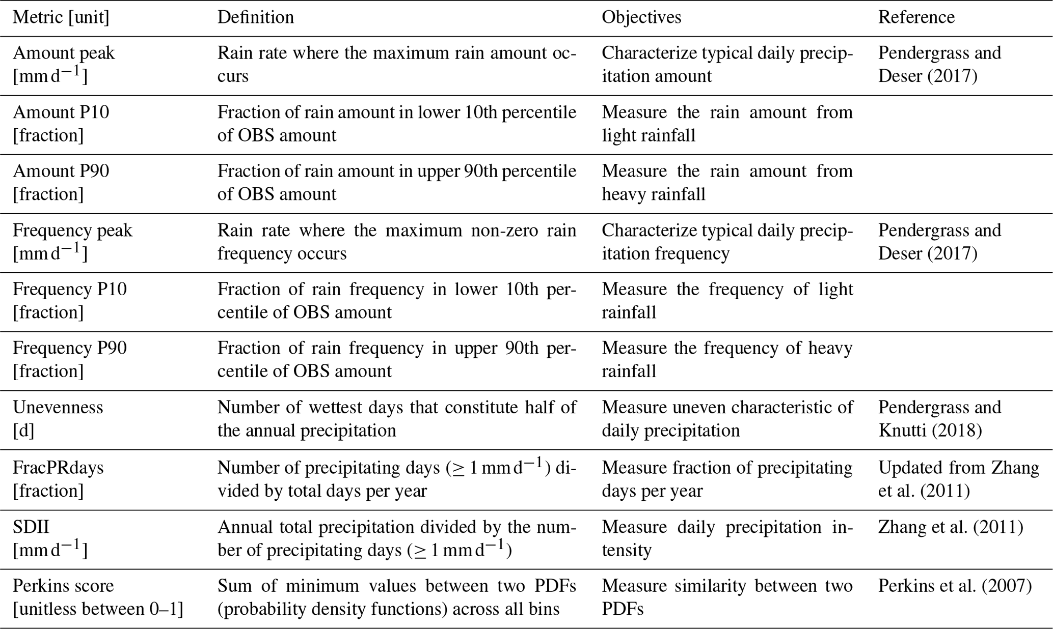
In our framework we apply 10 metrics that characterize different and complementary aspects of the intensity distribution of precipitation at regional scales. Table 3 summarizes the metrics including their definition, purpose, and references. The computation of the metrics has been implemented and applied in the PCMDI metrics package (PMP; Gleckler et al., 2008, 2016).

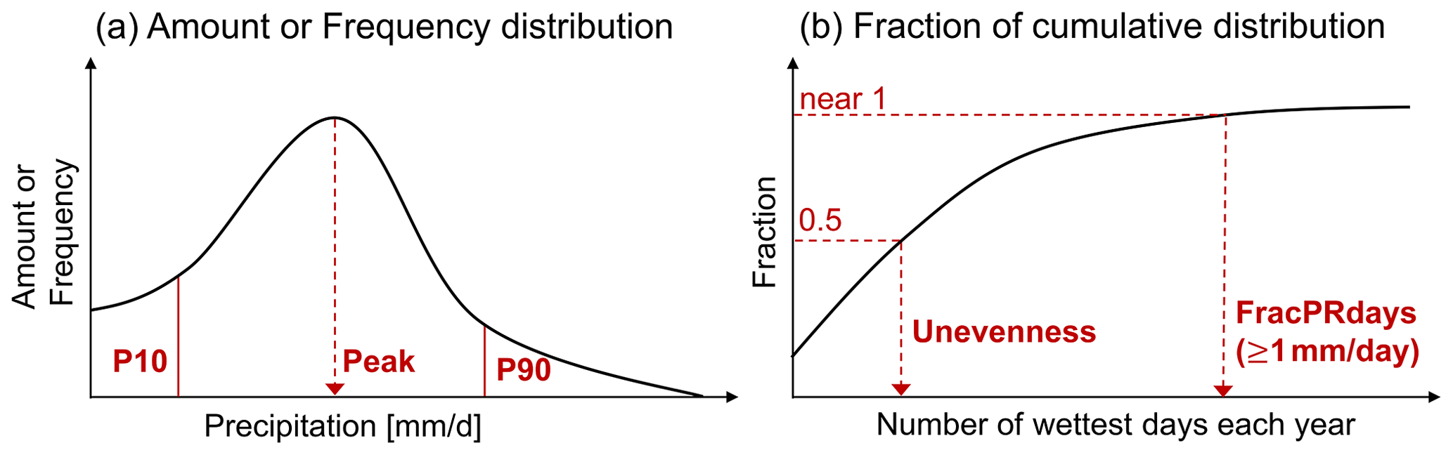
Figure 1 Schematics for precipitation distribution metrics. (a) Amount or Frequency distribution as a function of rain rate. Peak metric gauges the rain rate where the maximum distribution occurs. P10 and P90 metrics, respectively, measure the fraction of the distribution lower 10th percentile and upper 90th percentile. Perkins score is another metric based on the frequency distribution to quantify the similarity between observed and modeled distribution. (b) Fraction of cumulative distribution as a function of the number of wettest days. Unevenness gauges the number of wettest days for half of the annual precipitation. FracPRdays measures the fraction of the number of precipitating (≥ 1 mm d⁻¹) days per year. SDII is designed to measure daily precipitation intensity by annual total precipitation divided by FracPRdays.

3.1 Frequency and amount distributions

Following Pendergrass and Hartmann (2014) and Pendergrass and Deser (2017), we use logarithmically spaced bins of daily precipitation to calculate both the precipitation frequency and amount distributions. Each bin is 7 % wider than the previous one, and the smallest non-zero bin is centered at 0.03 mm d⁻¹. The frequency distribution is the number of days in each bin normalized by the total number of days, and the amount distribution is the sum of accumulated precipitation in each bin normalized by the total number of days. Based on these distributions (Fig. 1a), we identify the rain rate where the maximum peak of the distribution appears (Amount and Frequency peak; Pendergrass and Deser, 2017, also called mode; Kooperman et al., 2016) and formulate several complementary metrics that measure the fraction of the distribution's lower 10th percentile (P10) and upper 90th percentile (P90). The precipitation bins less than 0.1 mm d⁻¹ are considered dry for the purpose of these calculations. The threshold rain rates for the 10th and 90th percentiles are defined from the amount distribution as determined from observations. Here we use IMERG as the default reference observational dataset. The final frequency-related metric we employ is the Perkins score, which measures the similarity between observed and modeled frequency distributions (Perkins et al., 2007). With the sum of a frequency distribution across all bins being unity, the Perkins score is defined as the sum of minimum values between observed and modeled frequency across all bins: Perkins score = ${\sum }_{\mathrm{1}}^n\text{minimum }(Z_{\mathrm{o}},Z_{\mathrm{m}})$, where n is the number of bins, and Z_o and Z_m are the frequency in a given bin for observation and model, respectively. The Perkins score is a unitless scalar varying from 0 (low similarity) to 1 (high similarity).

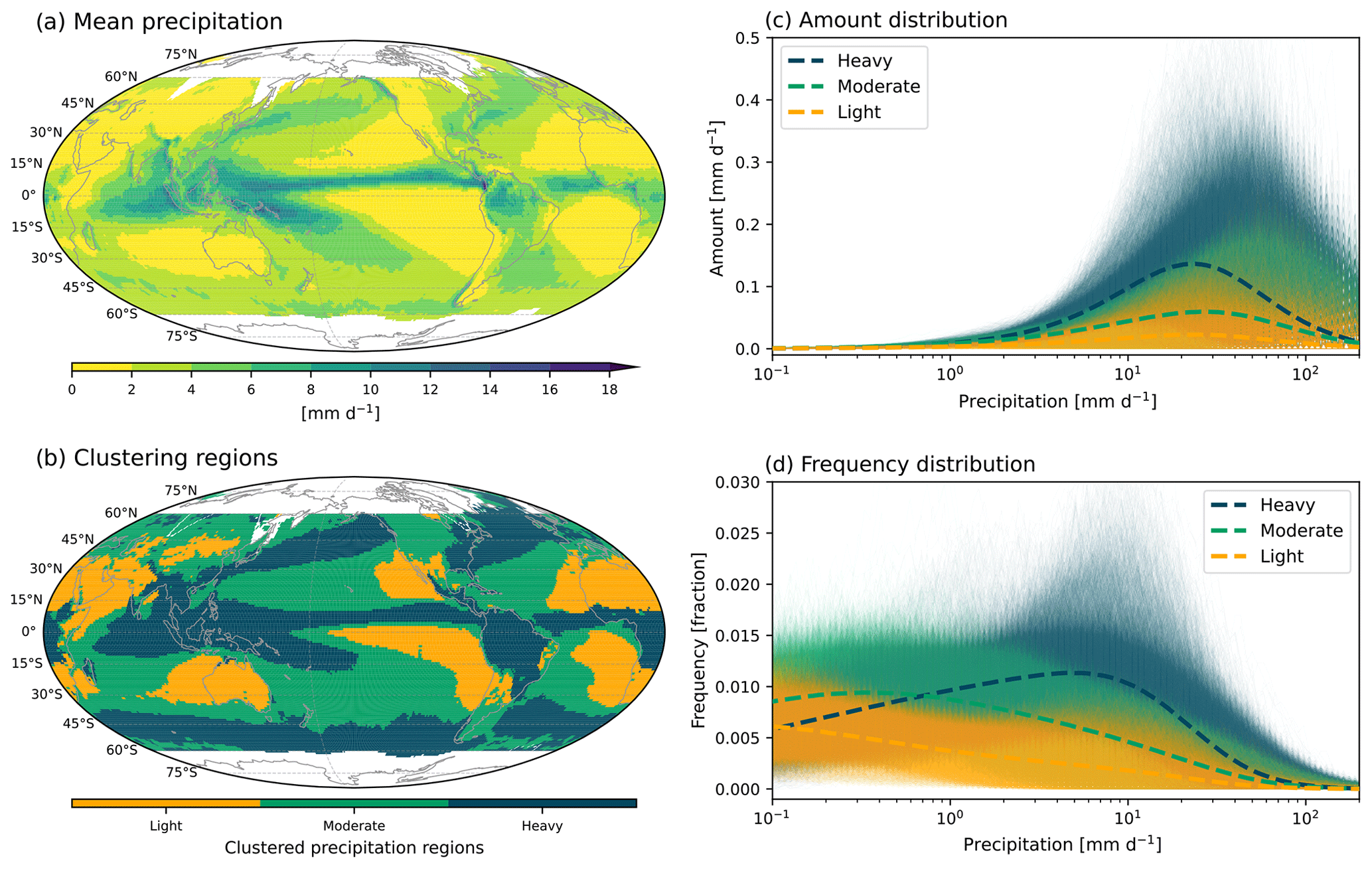
Figure 2 Spatial patterns of IMERG precipitation (a) mean state and (b) clustering for heavy-, moderate-, and light-precipitating regions by K-means clustering with amount and frequency distributions. Precipitation (c) amount and (d) frequency distributions as a function of rain rate. Different colors indicate different clustering regions and are the same as in (b). Thin and thick curves, respectively, indicate distributions at each grid and the cluster average.

3.2 Cumulative fraction of annual precipitation amount

Following Pendergrass and Knutti (2018), we calculate the cumulative sum of daily precipitation each year sorted in descending order (i.e., wettest to driest) and normalized by the total precipitation for that year. From the distribution for each individual year (see Fig. 1b), we obtain the metrics gauging the number of wettest days for half of the annual precipitation (Unevenness; Pendergrass and Knutti, 2018) and the fraction of the number of precipitating (≥1 mm d⁻¹) days (FracPRdays). To facilitate comparison against longer-established analyses (e.g., ETCCDI; Zhang et al., 2011), we include the daily precipitation intensity, calculated by dividing the annual total precipitation by the number of precipitating days (SDII; Zhang et al., 2011). To obtain values of these metrics over multiple years, we take the median across years following Pendergrass and Knutti (2018; for unevenness).

3.3 Reference regions

We use the spatial homogeneity of precipitation characteristics as a basis for defining regions, as in previous studies (e.g., Swenson and Grotjahn, 2019). In addition to providing more physically based results, this also simplifies interpretation with robust diagnostics when we average a distribution characteristic across the region. We use K-means clustering (MacQueen, 1967) with the concatenated frequency and amount distributions of IMERG over the global domain to identify homogeneous regions for precipitation distributions. K-means clustering is an unsupervised machine learning algorithm that separates characteristics of a dataset into a given number of clusters without explicitly provided criteria. This method has been widely used because it is faster and simpler than other methods. Here, we use three clusters to define heavy-, moderate-, and light-precipitating regions. Figure 2 shows the spatial pattern of IMERG precipitation mean state and clustering results defining heavy- (blue), moderate- (green), and light-precipitating (orange) regions. The spatial pattern of these clustering regions resembles the pattern of the mean state of precipitation, providing a sanity check indicating that the cluster-based regions are physically reasonable. Note that the clustering result with frequency and amount distributions is not significantly altered if we incorporate the cumulative amount fraction. However, the inclusion of the cumulative amount fraction to the clustering yields a slightly noisier pattern, and thus we have chosen to use the clustering result only with frequency and amount distributions.

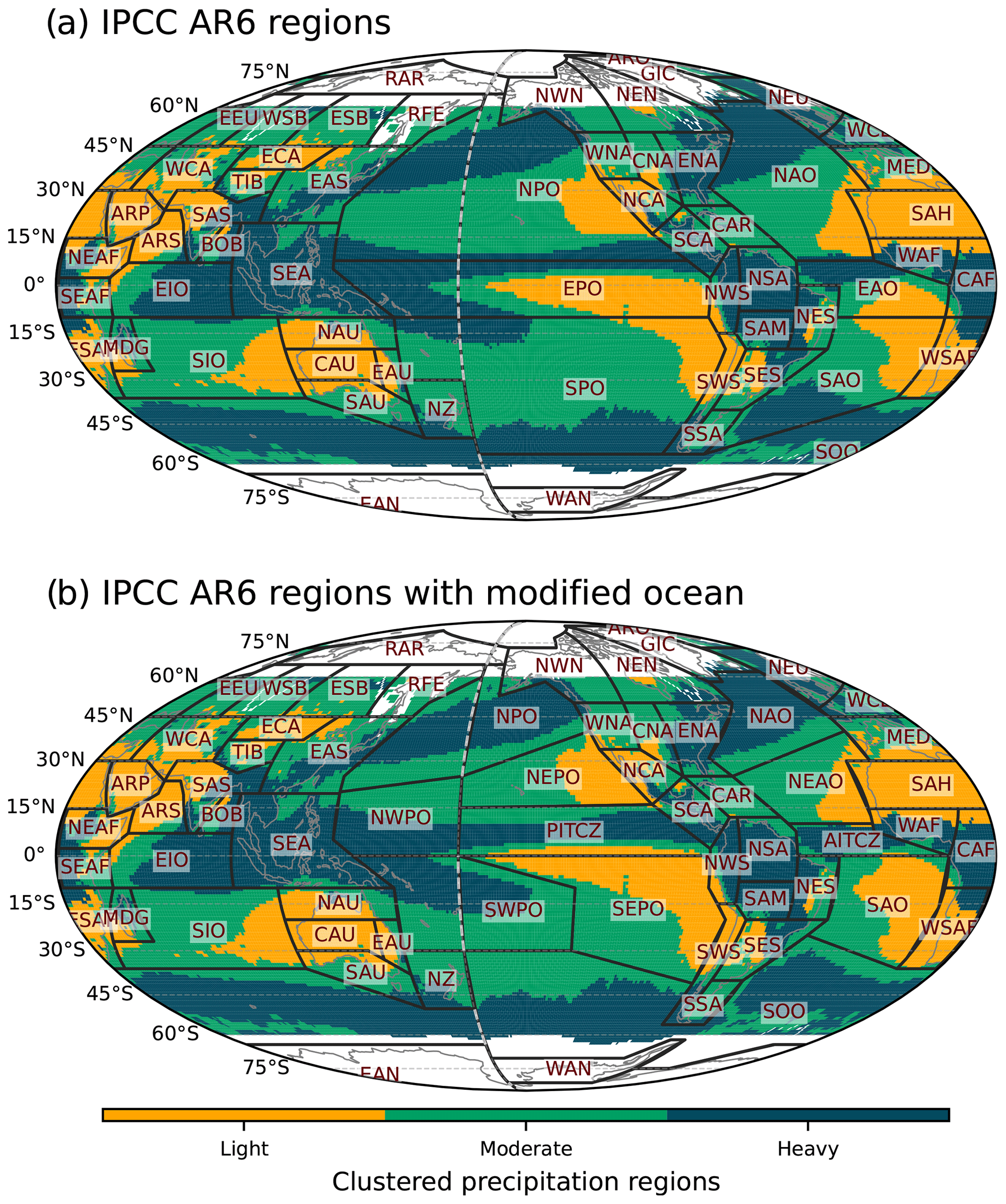
Figure 3 (a) IPCC AR6 climate reference regions and (b) modified IPCC AR6 climate reference regions superimposed on the precipitation distribution clustering map shown in Fig. 2b. Land regions are the same between (a) and (b), while some ocean regions are modified.

In support of the AR6, the IPCC proposed a set of climate reference regions (Iturbide et al., 2020). These regions were defined based on geographical and political boundaries and the climatic consistency of temperature and precipitation in current climate and climate change projections. When defining regions, the land regions use information from both current climate and climate change projections, while the ocean regions use only the information from climate change projections. In other words, the climatic consistency of precipitation in the current climate is not explicitly represented in the definition of the oceanic regions. Figure 3a shows the IPCC AR6 climate reference regions superimposed on our precipitation clustering regions shown in Fig. 2b. The land regions correspond reasonably well to the clustering regions, but some ocean regions are too broad, including both heavy- and light-precipitating regions (Fig. 3a). In this study, the ocean regions are modified based on the clustering regions, while the land regions remain the same as in the AR6 (Fig. 3b).

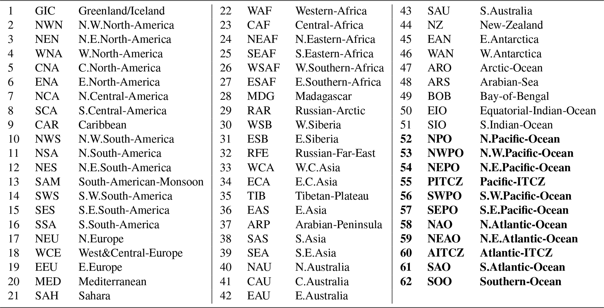
Table 4 List of climate reference regions used in this study. The new ocean regions defined in this study are highlighted in bold.

In the Pacific Ocean region, the original IPCC AR6 regions consist of equatorial Pacific Ocean (EPO), northern Pacific Ocean (NPO), and southern Pacific Ocean (SPO). Each of these regions includes areas of both heavy and light precipitation. EPO includes the Intertropical Convergence Zone (ITCZ), the South Pacific Convergence Zone (SPCZ), and also the dry southeast Pacific region. The NPO region includes the north Pacific storm track and the dry northeast Pacific. The SPO region includes the southern part of the SPCZ and the dry southeast area of the Pacific. In our modified IPCC AR6 regions, the Pacific Ocean region is divided into four heavy-precipitating regions (NPO, NWPO, PITCZ, and SWPO) and two light- and moderate-precipitating regions (NEPO and SEPO). Similarly, in the Atlantic Ocean region, the original IPCC AR6 regions consist of the equatorial Atlantic Ocean (EAO), northern Atlantic Ocean (NAO), and southern Atlantic Ocean (SAO), with each including both heavy- and light-precipitating regions. Our modified Atlantic Ocean region consists of two heavy-precipitating regions (NAO and AITCZ) and two light- and moderate-precipitating regions (NEAO and SAO). The Indian Ocean (IO) region is not modified as the original IPCC AR6 climate reference region separates well the heavy-precipitating equatorial IO (EIO) region from the moderate- and light-precipitating southern IO (SIO) region. The Southern Ocean (SOO) is modified to mainly include the heavy-precipitating region around the Antarctic. The original IPCC AR6 climate reference regions consist of 58 regions including 12 oceanic regions and 46 land regions, while our modification consists of 62 regions including 16 oceanic regions and the same land regions as the original (see Table 4). Note that the Caribbean (CAR), the Mediterranean (MED), and Southeast Asia (SEA) are not counted for the oceanic regions.

3.4 Evaluating model performance

We use two simple measures to compare the collection of CMIP5 and 6 model simulations with the five satellite-based observational products (IMERG, TRMM, CMORPH, GPCP, and PERSIANN). One gauges how many models within the multi-model ensemble fall within the observational range between the minimum and maximum observed values for each metric and each region. Another is how many models underestimate or overestimate all observations, i.e., are outside the bounds spanned by the minimum and maximum values across the five satellite-based products. To quantify the dominance of underestimation versus overestimation of the multi-model ensemble with a single number, we use the following measure formulation: $(\mathrm{nO}-\mathrm{nU})/\mathrm{nT}$, where nO is the number of overestimating models, nU is the number of underestimating models, and nT is the total number of models. Thus, positive values represent overestimation, and negative values represent underestimation. If models are mostly within the observational range or widely distributed from underestimation to overestimation, the quantification value would approach zero.

Many metrics that can be used to characterize precipitation, including those used here, are sensitive to the spatial and temporal resolutions at which the model and observational data are analyzed (e.g., Pendergrass and Knutti, 2018; Chen and Dai, 2019). As in many previous studies on the diagnosis of precipitation in CMIP5 and 6 models (e.g., Fiedler et al., 2020; Tang et al., 2021; Ahn et al., 2022), to ensure appropriate comparisons, we conduct all analyses at a common horizontal grid of 2^∘ × 2^∘ with a conservative regridding method. For models with multiple ensemble members, we first compute the metrics for all available realizations and then average the results across the realizations.

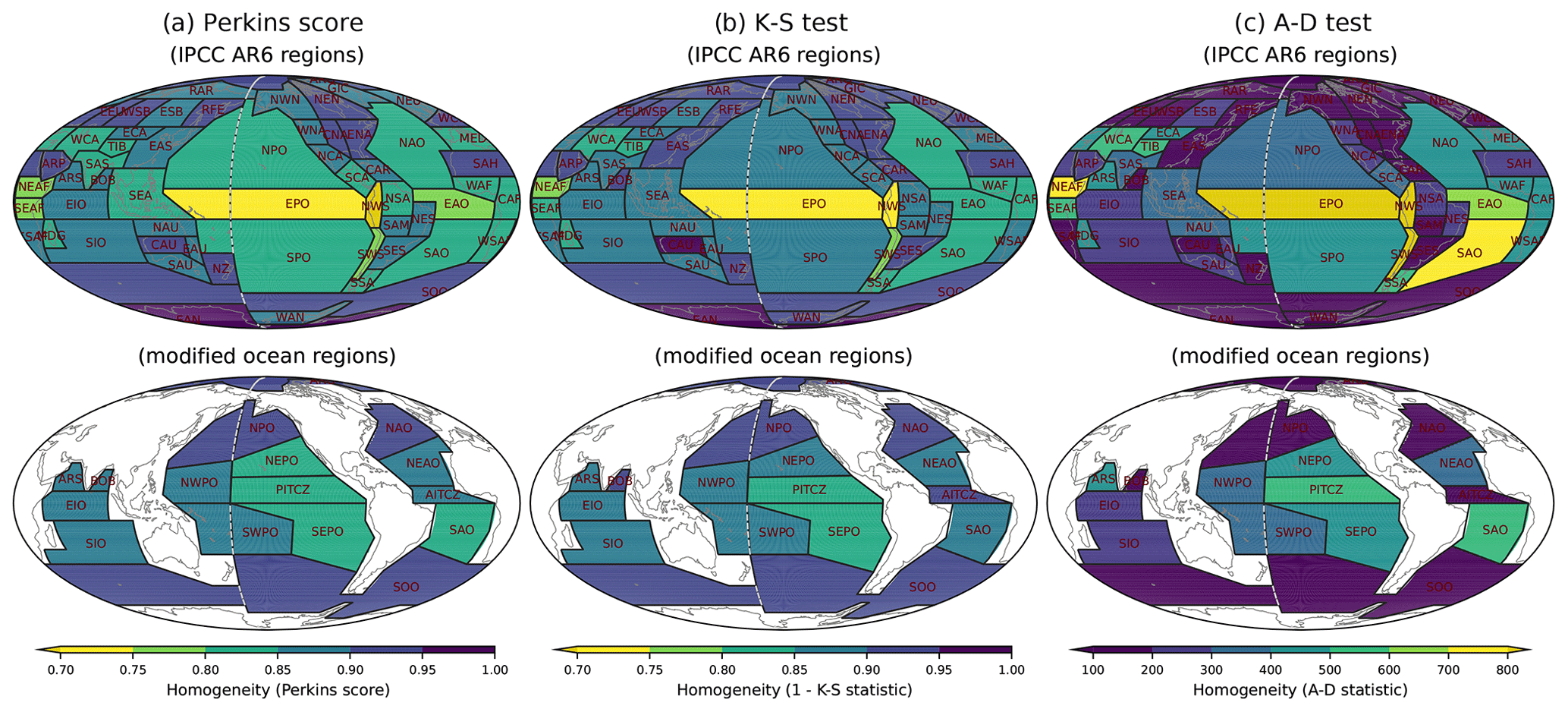
Figure 4 Homogeneity estimated by (a) Perkins score, (b) K-S test, and (c) A-D test between the region-averaged and each grid's frequency distributions of IMERG precipitation for the IPCC AR6 climate reference regions (upper) and the modified ocean regions (bottom). The darker color indicates higher homogeneity across all panels.

4 Results

4.1 Homogeneity within reference regions

For the regional-scale analysis, we employ the IPCC AR6 climate reference regions (Iturbide et al., 2020), while we revise the regional divisions over the oceans based on clustered precipitation characteristics as described in Sect. 3.3. To quantitatively evaluate the homogeneity of precipitation distributions in the reference regions, we use three homogeneity metrics: the Perkins score (Perkins et al., 2007), Kolmogorov–Smirnov test (K-S test; Chakravart et al., 1967), and Anderson–Darling test (A-D test; Stephens, 1974). The three metrics measure the similarity between the regionally averaged and individual grid cell frequency distributions within the region. The Perkins score measures the overall similarity between two frequency distributions, which is one of our distribution performance metrics described in Sect. 3.1. The K-S and A-D tests focus more on the similarity in the center and the side of the frequency distribution, respectively. The three homogeneity metrics could complement each other as their main focuses are on different aspects of frequency distributions.

Figure 5 As in Fig. 4 but for different observational datasets with Perkins score.

In the original IPCC AR6 reference regions, the oceanic regions show relatively low homogeneity of precipitating characteristics compared to land regions (Fig. 4). The Pacific and Atlantic Ocean regions show much lower homogeneity than the Indian Ocean, especially in EPO and EAO regions. In the modified oceanic regions, the homogeneities show an overall improvement with the three homogeneity metrics. In particular, the homogeneity over the heavy-precipitating regions where the homogeneity was lower (e.g., Pacific and Atlantic ITCZ and midlatitude storm track regions) are largely improved. The clustering regions shown here are obtained based on IMERG precipitation. However, since different satellite-based products show substantial discrepancies in precipitation distributions, it is important to assess whether the improved homogeneity in the modified regions is similarly improved across other different datasets. Figure 5 shows the homogeneity of precipitation distribution characteristics for different observational datasets using the Perkins score. Although the region modifications we have made are based on the clustering regions of IMERG precipitation, Fig. 5 suggests that the improvement of the homogeneity over the modified regions is consistent across different observational datasets. We further tested the homogeneity for different seasons (see Fig. S1 in the Supplement). The homogeneity is overall improved in the modified regions across the seasons even though we defined the reference regions based on annual data.

Figure 6 Precipitation amount (a, d, and g), frequency (b, e, and h), and cumulative (c, f, and i) distributions for (a–c) NWPO, (b–f) SEPO, and (g–j) ENA. Black, gray, blue, and red curves indicate the satellite-based observations, reanalysis, CMIP5 models, and CMIP6 models, respectively. Thin and thick curves for CMIP models, respectively, indicate distributions for each model and multi-model average. Gray dotted lines in the cumulative distributions indicate a fraction of 0.5. Note: all model output and observations were conservatively regridded to 2^∘ in the first step of analysis.

4.2 Regional evaluation of model simulations against multiple observations

The precipitation distribution metrics used in this study are mainly calculated from three curves: amount distribution, frequency distribution, and cumulative amount fraction curves. Figure 6 shows these curves for three selected regions based on the clustered precipitating characteristics (NWPO, which is a heavy-precipitation-dominated ocean region; SEPO, a light-precipitation-dominated ocean region; and ENA, a heavy-precipitation-dominated land region). The heavy- and light-precipitating regions are well distinguished by their overlaid distribution curves. The amount distribution has a distinctive peak in the heavy-precipitating region (Fig. 6a and g), while it is flatter in the light-precipitating region (Fig. 6d). The frequency distribution is more centered on the heavier precipitation side in the heavy-precipitating region (Fig. 6b and h) than in the light-precipitating region (Fig. 6e). The cumulative fraction increases more steeply in the light-precipitating region (Fig. 6f) than in the heavy-precipitating region (Fig. 6c and i), indicating there are fewer precipitating days in the light-precipitating region. NWPO and SEPO were commonly averaged for representing the tropical ocean region in many studies, but these different characteristics in the precipitation distributions demonstrate the additional information available via a regional-scale analysis. Although satellite-based observations are less reliable over the light-precipitating ocean regions (e.g., SEPO), the differences between heavy- and light-precipitating regions are well distinguishable.

In the precipitation frequency distribution, many models show a bimodal distribution in the heavy-precipitating tropical ocean region (Fig. 6b) but not in the light-precipitating subtropical ocean region (Fig. 6e) or the heavy-precipitating midlatitude land region (Fig. 6h). The bimodal frequency distribution is commonly found in models and is seemingly independent of resolution (e.g., Lin et al., 2013; Kooperman et al., 2018; Chen et al., 2021; Ma et al., 2022; Martinez-Villalobos et al., 2022; Ahn et al., 2023). Ma et al. (2022) compared the frequency distributions in AMIP and HighResMIP (High Resolution Model Intercomparison Project; Haarsma et al., 2016) from CMIP6 and DYAMOND (DYnamics of the Atmospheric general circulation Modeled On Non-hydrostatic Domains; Satoh et al., 2019; Stevens et al., 2019) models, where they showed that the bimodal frequency distribution appears in many AMIP (∼ 100 km), HighResMIP (∼ 50 km), and even DYAMOND (∼ 4 km) models. Ahn et al. (2023) further compared DYAMOND model simulations with and without a convective parameterization and showed that most DYAMOND model simulations exhibiting the bimodal distribution use a convective parameterization. ERA5 reanalysis also shows a bimodal frequency distribution (Fig. 6b), which is not surprising considering that the reproduced precipitation in ERA5 heavily depends on the model, and thus exhibits this common model behavior. Because of the heavy reliance on model physics to generate its precipitation (as opposed to fields like wind, for which observations are directly assimilated), in this study we do not include ERA5 precipitation among the observational products used for model evaluation.

Figure 7 Precipitation distribution metrics for (a) Amount peak, (b) Amount P10, (c) Amount P90, (d) Frequency peak, (e) Frequency P10, (f) Frequency P90, (g) Unevenness, (h) FracPRdays, (i) SDII, and (j) Perkins score over the modified IPCC AR6 regions. Black, gray, blue, and red markers indicate the satellite-based observations, reanalysis, CMIP5 models, and CMIP6 models, respectively. Thin and thick vertical marks for CMIP models, respectively, indicate distributions for each model and multi-model average. The open circle mark for CMIP models indicates the multi-model median. The green shade represents the range between the minimum and maximum values of satellite-based observations. Blue and red shades, respectively, represent the range between the 25th and 75th model values for CMIP5 and 6 models. The y axis labels are shaded with the same three colors as in Fig. 2b, indicating dominant precipitating characteristics. Note that regions 1–46 are land and land–ocean mixed regions and 47–62 are ocean regions.

Based on the precipitation amount, frequency, and cumulative amount fraction curves, we calculate 10 metrics (Amount peak, Amount P10, Amount P90, Frequency peak, Frequency P10, Frequency P90, Unevenness, FracPRdays, SDII, and Perkins score) as described in Sect. 3. Figure 7 shows the metrics with the modified IPCC AR6 climate reference regions for satellite-based observations (black), ERA5 reanalysis (gray), CMIP5 models (blue), and CMIP6 models (red). The metric values vary widely across regions, especially in Amount peak, Frequency peak, Unevenness, FracPRdays, and SDII, demonstrating the additional detail provided by regional-scale precipitation distribution metrics. In terms of the metrics based on the amount distribution (Fig. 7a–c), many models tend to simulate an Amount peak that is too light, an Amount P10 that is too high, and an Amount P90 that is too low compared to the observations, more so in oceanic regions (regions 47–62) than in land regions. Similarly for the metrics based on the frequency distribution (Fig. 7d–f), many models show light Frequency peaks, overestimated Frequency P10, and underestimated Frequency P90 compared to observations. The similarity between frequency distribution curves (i.e., Perkins score) is higher in land regions than in ocean regions. Also, many models overestimate Unevenness and FracPRdays and underestimate SDII. These results indicate that, overall, models simulate more frequent weak precipitation and less heavy precipitation compared to the observations, consistent with many previous studies (e.g., Dai, 2006; Pendergrass and Hartmann, 2014; Trenberth et al., 2017; Chen et al., 2021; Ma et al., 2022).

Figure 8 Observational discrepancies relative to spread in the multi-model ensemble for (a) Amount peak, (b) Amount P10, (c) Amount P90, (d) Frequency peak, (e) Frequency P10, (f) Frequency P90, (g) Unevenness, (h) FracPRdays, (i) SDII, and (j) Perkins score over the modified IPCC AR6 regions. The observational discrepancy is calculated by the standard deviation of satellite-based observations divided by the standard deviation of CMIP5 and 6 models for each metric and region.

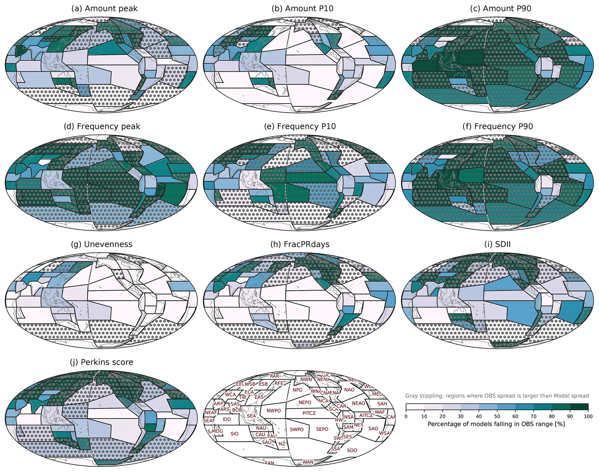
Figure 9 Percentage of CMIP6 models within range of the observational products for (a) Amount peak, (b) Amount P10, (c) Amount P90, (d) Frequency peak, (e) Frequency P10, (f) Frequency P90, (g) Unevenness, (h) FracPRdays, (i) SDII, and (j) Perkins score over the modified IPCC AR6 regions. The observational range is between the minimum and maximum values of five satellite-based products. Regions where the observational spread is larger than model spread shown in Fig. 8 are stippled gray.

As expected from previous work, observations disagree substantially in some regions (e.g., polar and high-latitude regions) and/or for some metrics (e.g., Amount P90, Frequency P90). In some cases the observational spread is much larger than that of the models. We examine the observational discrepancy or spread by the ratio between the standard deviation of the five satellite-based observations (IMERG, TRMM, CMORPH, GPCP, PERSIANN) and the standard deviation of all CMIP5 and 6 models (Fig. 8). The standard deviation of observations is much larger near polar regions and high-latitude regions compared to the models' standard deviation for most metrics, as expected from the orbital configurations of the most relevant satellite constellations for precipitation (which exclude high latitudes). The Amount P90 and Frequency P90 metrics show the largest observational discrepancy among the metrics, with standard deviations 1.5 to 3 times larger over some high-latitude regions and about 3–8 times larger over polar regions in observations compared to the models. On the other hand, Unevenness, FracPRdays, and Amount P10 show the least observational discrepancy – the models' standard deviation is about 2–8 times larger than for observations over some tropical and subtropical regions; nonetheless, the standard deviation among observations is larger over most of the high-latitude and polar regions. Model evaluation in the regions with large disagreement among observational products remains a challenge. Note that the standard deviation of five observations would be sensitive as there are outlier observations for some regions and metrics (e.g., many ocean regions in Amount P90). Moreover, observational uncertainties are rarely well quantified or understood, so agreements among observational datasets may not always allow us to rule out common errors among observations (e.g., for warm light precipitation over the subtropical ocean).

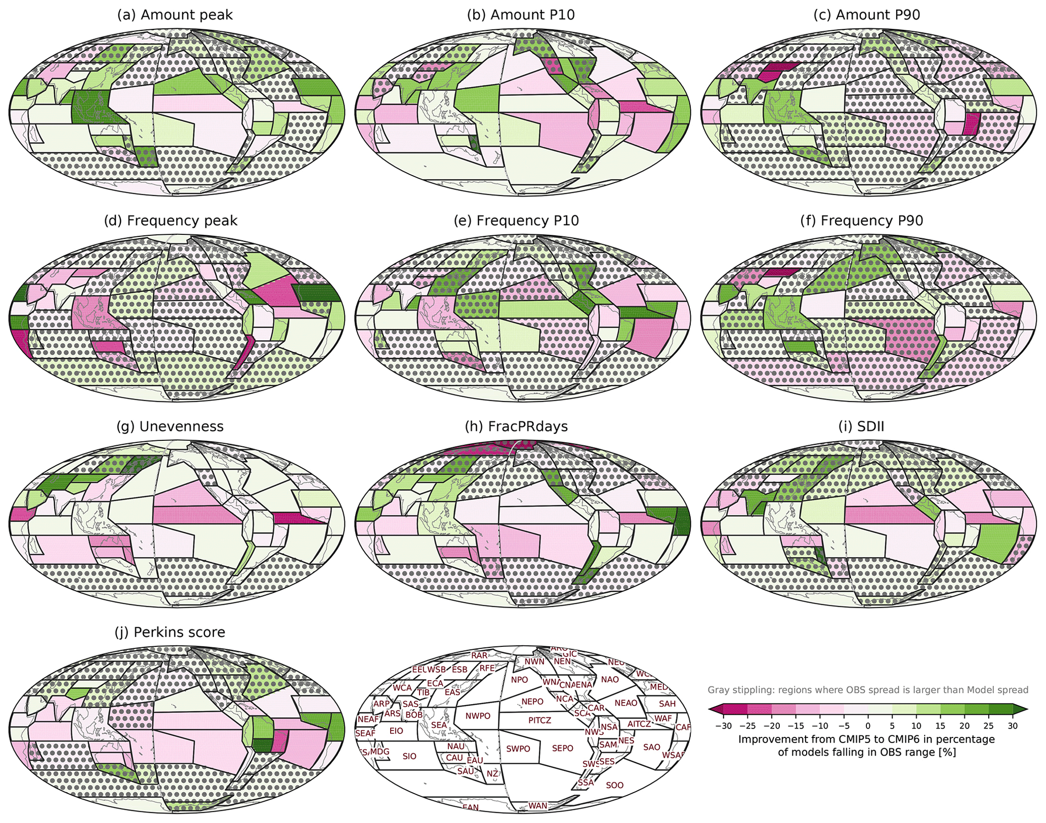
Figure 10 Improvement from CMIP5 to 6 as identified by the percentage of models in each multi-model ensemble that are within the observational min-to-max range. The improvement is calculated by the CMIP6 percentage minus the CMIP5 percentage so that positive and negative values, respectively, indicate improvement and deterioration in CMIP6. Regions where the observational spread is larger than model spread are stippled gray.

To attempt to account for discrepancies among observational datasets in the model evaluation framework, we use two different approaches to evaluate model performance with multiple observations, as described in Sect. 3.4. The first approach is to assess the number of models that are within the observational range. Figure 9 shows the CMIP6 model evaluation with each metric, and the regions where the standard deviation among observations is larger than among models are stippled gray to avoid them in the model performance evaluation. In Amount peak, some subtropical regions (e.g., ARP, EAS, NEPO, CAU, and WSAF) show relatively good model performance (more than 70 % of models fall in the observational range), while some tropical and subtropical (e.g., PITCZ, AITCZ, and SEPO) and polar (e.g., RAR, EAN, and WAN) regions show poor model performance (less than 30 % of models fall in observational range). For Amount P10, many regions are poorly captured by the simulations, except for some subtropical land regions (e.g., EAS, NCA, CAU, and WSAF). In Amount P90, most regions are uncertain (i.e., the standard deviation among observations is larger than among models) making it difficult to evaluate model performance, while some tropical regions near the Indo-Pacific warm pool (EIO, SEA, NWPO, and NAU) exhibit very good model performance (more than 90 % of models fall in observational range). In the Frequency metrics (peak, P10, and P90), it is difficult in more regions to evaluate model performance than in Amount metrics, while in some tropical and subtropical regions (e.g., PITCZ, SWPO, NWPO, SEA, SAO, and NES) model performance is good. However, good model performance could alternatively arise from a large observational range (see Fig. 7). Unevenness, FracPRdays, SDII, and Perkins score have a smaller fraction of models within the observational range in tropical regions than the Amount and Frequency metrics. In particular, fewer than 10 % of CMIP6 models fall within the observational range for Unevenness and FracPRdays over some tropical oceanic regions (e.g., PITCZ, NEPO, SEPO, AITCZ, NEAO, SAO, and SIO).

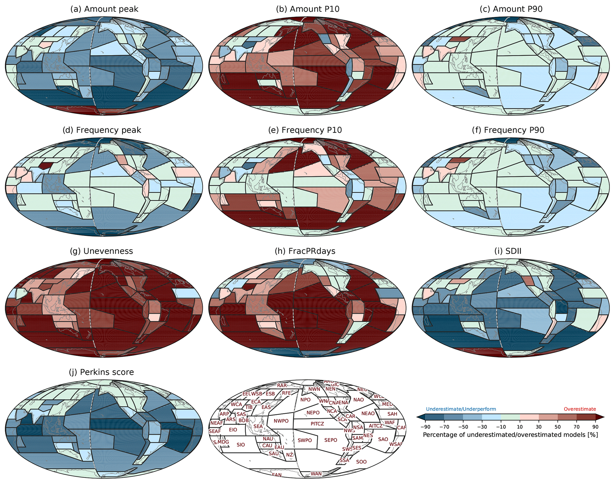
Figure 11 Percentage of CMIP6 models underestimating or overestimating observations for (a) Amount peak, (b) Amount P10, (c) Amount P90, (d) Frequency peak, (e) Frequency P10, (f) Frequency P90, (g) Unevenness, (h) FracPRdays, (i) SDII, and (j) Perkins score over the modified IPCC AR6 regions. The criteria for underestimation and overestimation are, respectively, defined by minimum and maximum values of satellite-based observations shown in Fig. 7. Positive and negative values, respectively, represent overestimation and underestimation by a formulation of $(\mathrm{nO}-\mathrm{nU})/\mathrm{nT}$ where nO, nU, and nT are, respectively, the number of overestimated models, underestimated models, and total models.

Examining the fraction of CMIP5 models falling within the range of observations, CMIP5 models have a spatial pattern of model performance similar to that of CMIP6 models (see Fig. S2), and the improvement from CMIP5 to CMIP6 seems subtle. We quantitatively assess the improvement from CMIP5 to CMIP6 by subtracting the percentage of CMIP5 from CMIP6 models falling within the range of observations (Fig. 10). For some metrics (e.g., Amount peak, Amount and Frequency P10, and Amount and Frequency P90) and for some tropical and subtropical regions (e.g., SEA, EAS, SAS, ARP, and SAH), the improvement is apparent. Compared to CMIP5, 5 %–25 % more CMIP6 models fall in the observational range in these regions. However, for the other metrics (e.g., Frequency peak, FracPRdays, SDII, Perkins score), CMIP6 models perform somewhat worse. Over some tropical and subtropical oceanic regions (e.g., PITCZ, NEPO, AITCZ, and NEAO), 5 %–25 % more CMIP6 than CMIP5 models are out of the observational range. This result is from all available CMIP5 and CMIP6 models, so it may reflect the fact that some models are in only CMIP5 or CMIP6 but not both (see Table 2). To isolate improvements that may have occurred between successive generations of the same models, we also compared only the models that participated in both CMIP5 and CMIP6 (see Fig. S3). Overall, the spatial characteristics of the improvement/degradation in CMIP6 from CMIP5 are consistent, while more degradation is apparent when we compare this subset of models, especially over the tropical oceanic regions (e.g., PITCZ, AITCZ, NWPO, and SEPO).

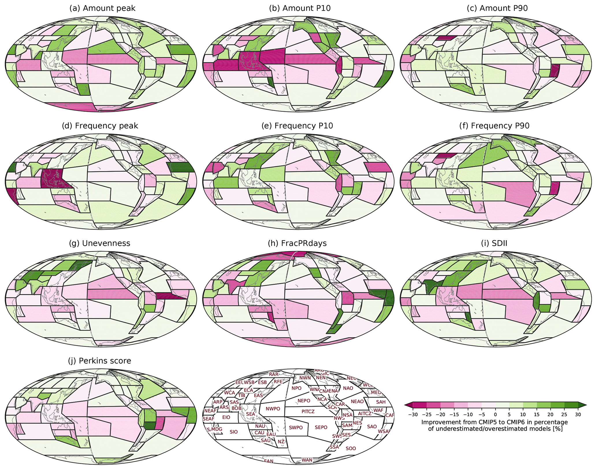
Figure 12 Improvement from CMIP5 to 6 in the percentage of underestimated or overestimated models. The improvement is calculated by the absolute value of CMIP5 percentage minus the absolute value of CMIP6 percentage so that positive and negative values, respectively, indicate improvement and deterioration in CMIP6.

The second approach to account for discrepancies among observations in model performance evaluation is to count the number of models that are lower or higher than all satellite-based observations for each metric and each region. Figure 11 shows the spatial patterns of the model performance evaluation with each metric for CMIP6 models. Underestimation is indicated by a negative sign, while overestimation is indicated by a positive sign via the formulation described in Sect. 3.4. Amount peak is overall underestimated in most regions, indicating the amount distributions in most CMIP6 models are shifted to lighter precipitation compared to observations. In many regions, more than 50 % of the CMIP6 models underestimate Amount peak. In particular, over many tropical and Southern Hemisphere ocean regions (e.g., PITCZ, AITCZ, EIO, SEPO, SAO, and SOO), more than 70 % of the models underestimate the Amount peak. The underestimation of Amount peak is accompanied by overestimation of Amount P10 and underestimation of Amount P90. More than 70 % of CMIP6 models overestimate Amount P10 in many oceanic regions; especially in the southern and northern Pacific and Atlantic, the southern Indian Ocean, and Southern Ocean more than 90 % of the models overestimate the observed Amount P10. For Amount P90, it appears that many models fall within the observational range; however, the observational range in Amount P90 (green boxes in Fig. 7c) is large and driven primarily by just one observational dataset (IMERG), especially in ocean regions.

For the frequency-based metrics (i.e., peak, P10, and P90; Fig. 11d–f), CMIP6 models show similar bias characteristics to Amount metrics (Fig. 11a–c), although performance is better than for Amount metrics. Over some tropical (e.g., NWPO, PITCZ, and SWPO ) and Eurasian (e.g., EEU, WSB, and ESB) regions, less than 10 % of models fall outside of the observed range. Unevenness and FracPRdays are severely overestimated in models. More than 90 % of models overestimate the observed Unevenness (Fig. 11g) and FracPRdays (Fig. 11h) globally, especially over oceanic regions, consistent with Pendergrass and Knutti (2018). SDII is underestimated in many regions globally, especially in some heavy-precipitating regions (e.g., PITCZ, AITCZ, EIO, SEA, NPO, NAO, SWPO, and SOO). For the Perkins score, model simulations have poorer performance in the tropics than in the midlatitudes and polar regions. The performance of these various metrics is generally consistent with the often-blamed light precipitation that is too frequent and heavy precipitation that is too rare in simulations.

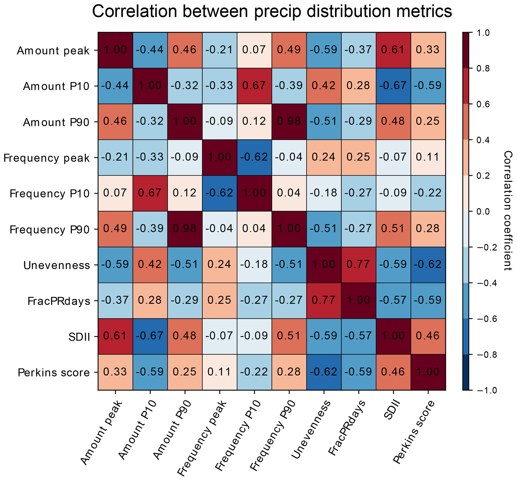
Figure 13 Correlation between precipitation distribution metrics across CMIP5 and 6 model performances. The correlation coefficients are calculated for the modified IPCC AR6 regions and then area-weight-averaged globally.

The characteristics of CMIP5 compared to CMIP6 simulations (Fig. S4) show little indication of improvement. Here we quantitatively evaluate the improvement in CMIP6 from CMIP5 for each metric and region. Figure 12 shows the difference between CMIP5 and CMIP6 in terms of the percentage of models that underestimate or overestimate each metric. In midlatitudes, there appears to have been an improvement in performance, however in the tropics, there appears to be more degradation. Over some heavy-precipitating tropical regions (e.g., PITCZ, AITCZ, EIO, and NWPO), 10 %–25 % more models in CMIP6 than in CMIP5 overestimate Amount P10, Unevenness, and FracPRdays and underestimate/underperform on Amount peak, SDII, and Perkins score. This indicates that CMIP6 models simulate more frequent light precipitation and less frequent heavy precipitation over the heavy-precipitating tropical regions. Over some midlatitude land regions (e.g., EAS, ESB, RFE, and ENA), on the other hand, 5 %–20 % more models in CMIP6 than in CMIP5 simulate precipitation distributions close to observations (i.e., less light precipitation and more heavy precipitation). To evaluate the improvement between model generation, we also compare only the models that participated in both CMIP5 and CMIP6 (Fig. S5) rather than all available CMIP5 and CMIP6 models. For the subset of models participating in both generations, the improvement characteristics are similar for all models, although more degradation is exhibited over some tropical oceanic regions (e.g., PITCZ, NWPO, and SWPO). This also indicates that some models newly participating in CMIP6, and not in CMIP5, have higher than average performance.

Figure 14 Scatterplot between 2^∘ and 4^∘ interpolated horizontal resolutions in evaluating precipitation distribution metrics for (a) Amount peak, (b) Amount P10, (c) Amount P90, (d) Frequency peak, (e) Frequency P10, (f) Frequency P90, (g) Unevenness, (h) FracPRdays, (i) SDII, and (j) Perkins score. The metric values are calculated for the modified IPCC AR6 regions and then weight-averaged globally. Black, gray, blue, and red marks indicate the satellite-based observations, reanalysis, CMIP5 models, and CMIP6 models, respectively. The number in the upper right of each panel is the correlation coefficient between the metric values in 2^∘ and 4^∘ resolutions across all observations and models.

4.3 Correlation between metrics

Each precipitation distribution metric implemented in this study is chosen to target different aspects of the distribution of precipitation. To the extent that precipitation probability distributions are governed by a small number of key parameters (as argued by Martinez-Villalobos and Neelin, 2019), we should expect additional metrics to be highly correlated. Figure 13 shows the global weighted average of correlation coefficients between the precipitation distribution metrics across CMIP5 and CMIP6 models. Higher correlation coefficients are found to be between Amount P90 and Frequency P90 (0.98) and between Amount P10 and Frequency P10 (0.67). This is expected because the amount and frequency distributions differ only by a factor of the precipitation rate (e.g., Pendergrass and Hartmann, 2014). Another higher correlation coefficient is between Unevenness and FracPRdays (0.77), indicating that the number of the heaviest-precipitating days for half of the annual precipitation and the total number of annual precipitating days are related. Amount and Frequency peak metrics are negatively correlated to P10 metrics and positively correlated to P90 metrics, but the correlation coefficients are not very high (lower than 0.62). This is because the peak metrics focus on typical precipitation rather than the light and heavy ends of the distribution that are the focus of P10 and P90 metrics. SDII is more negatively correlated with Amount P10 (−0.67) and positively correlated with Amount peak (0.61) and less so with Amount P90 (0.48), implying that SDII is mainly influenced by weak-precipitation amounts rather than heavy-precipitation amounts. The Perkins score shows relatively high negative correlation with Unevenness (−0.62), FracPRdays (−0.59), and Amount P10 (−0.59). This indicates that the discrepancy between the observed and modeled frequency distributions is partly associated with the overestimated light precipitation in models. The correlation coefficients between the metrics other than those discussed above are lower than 0.6. While there is some redundant information within the collection of metrics included in our framework, we retain all metrics so that others can select an appropriate subset for their own application. This also preserves the ability to readily identify outlier behavior of an individual model across a wide range of regions and statistics.

4.4 Influence of spatial resolution on metrics

Many metrics for the precipitation distribution are sensitive to the spatial resolution of the underlying data (e.g., Pendergrass and Knutti, 2018; Chen and Dai, 2019). Figure 14 shows how our results (which are all based on data at 2^∘ resolution) are impacted if we calculate the metrics from data coarsened to a 4^∘ grid instead. As expected, there is clearly some sensitivity to the spatial scale at which our precipitation distribution metrics are computed, but the correlation among datasets (both models and observations) between the two resolutions is very high, indicating that evaluations at either resolution should be consistent. At the coarser resolution, Amount peak and SDII are consistently smaller (as expected); Amount P10 and Frequency P10 tend to be smaller as well. Meanwhile, Unevenness and FracPRdays are consistently large (as expected); Amount P90, Frequency P90, and Perkins score are generally larger as well. Chen and Dai (2019) discussed a grid aggregation effect that is associated with the increased probability of precipitation as the horizontal resolution becomes coarser. This effect is clearly evident with increased Unevenness (Fig. 14g), FracPRdays (Fig. 14h), and decreased SDII (Fig. 14i) in coarser resolution. However, despite these differences, the relative model performance is not very sensitive to the spatial scale at which we apply our analysis. The correlation coefficients between results based on all data interpolated to 2 or 4^∘ horizontal resolution are above 0.9 for all of our distribution metrics. Conclusions on model performance are relatively insensitive to the target resolution.

5 Discussion

Analyzing the distribution of precipitation intensity lags behind temperature and even mean precipitation. Challenges include choosing appropriate metrics and analysis resolution to characterize this highly non-Gaussian variable and interpreting model skills in the face of substantial observational uncertainty. Comparing results derived at 2 and 4^∘ horizontal resolution for CMIP class models, we find that the quantitative changes in assessed performance are highly consistent across models and consequently have little impact on our conclusions. More work is needed to determine how suitable this collection of metrics may be for evaluating models with substantially higher resolutions (e.g., HighResMIP; Haarsma et al., 2016). We note that more complex measures have been designed to be scale independent (e.g., Martinez-Villalobos and Neelin, 2019; Martinez-Villalobos et al., 2022), and these may become increasingly important with continued interest in models developed at substantially higher resolution.

Several recent studies suggest that the IMERG represents a substantial advancement over TRMM and likely the others (e.g., Wei et al., 2017; Khodadoust Siuki et al., 2017; Zhang et al., 2018); thus we rely on IMERG as the default in much of our analysis. However, we do not entirely discount the other products because the discrepancy between them provides a measure of uncertainty in the satellite-based estimates of precipitation. Our use of the minimum to maximum range of multiple observational products is indicative of their discrepancy, but not their uncertainty, and thus is a limitation of the current work and challenge that we hope will be addressed in the future.

The common model biases identified in this study are mainly associated with the overestimated light precipitation and underestimated heavy precipitation. These biases persist from deficiencies identified in earlier-generation models (e.g., Dai, 2006), and as shown in this study there has been little improvement. One reason may be that these key characteristics of precipitation are not commonly considered in the model development process. Enabling modelers to more readily objectively evaluate simulated precipitation distributions could perhaps serve as a guide to improvement. The current study aims to provide a framework for the objective evaluation of simulated precipitation distributions at regional scales.

Imperfect convective parameterizations are a possible cause of the common model biases in precipitation distributions (e.g., Lin et al., 2013; Kooperman et al., 2018; Ahn and Kang, 2018; Chen and Dai, 2019; Chen et al., 2021; Martinez-Villalobos et al., 2022). Many convective parameterizations tend to produce precipitation that is too frequent and light, the so-called “drizzling” bias (e.g., Dai, 2006; Trenberth et al., 2017; Chen et al., 2021; Ma et al., 2022), and it is likely due to the fact that the parameterized convection is more readily triggered than that in nature (e.g., Lin et al., 2013; Chen et al., 2021). As model horizontal resolution increases, grid-scale precipitation processes can lead to resolving convective precipitation, as in so-called cloud-resolving, storm-resolving, or convective-permitting models. Ma et al. (2022) compare several storm-resolving models in DYAMOND to recent CMIP6 models with a convective parameterization and observe that the simulated precipitation distributions are more realistic in the storm-resolving models. However, some of the storm-resolving models still suffer from precipitation distribution errors, including bimodality in the frequency distribution. Further studies are needed to better understand the precipitation distribution biases in models.

6 Conclusion

We introduce a framework for the regional-scale evaluation of simulated precipitation distributions with 62 climate reference regions and 10 precipitation distribution metrics and apply it to evaluate the two most recent generations of climate model intercomparison simulations (i.e., CMIP5 and CMIP6).

To facilitate the regional scale for evaluation, regions where precipitation characteristics are relatively homogenous are identified. Our reference regions consist of existing IPCC AR6 climate reference regions, with additional subdivisions based on homogeneity analysis performed on precipitation distributions within each region. Our precipitation clustering analysis reveals that the IPCC AR6 land regions are reasonably homogeneous in precipitation character, while some ocean regions are relatively inhomogeneous, including large portions of both heavy- and light-precipitating areas. To define more homogeneous regions for the analysis of precipitation distributions, we have modified some ocean regions to better fit the clustering results. Although the clustering regions are obtained based on the IMERG annual precipitation, the improved homogeneity is fairly consistent across different datasets (TRMM, CMORPH, GPCP, PERSIANN, and ERA5) and seasons (March–May, MAM; June–August, JJA; September–November, SON; and December–February, DJF). The use of these more homogeneous regions enables us to extract more robust quantitative information from the distributions in each region.

To form the basis for evaluation within each region, we use a set of metrics that are well-established and easy to interpret, aiming to extract key characteristics from the distributions of precipitation frequency, amount, and cumulative fraction of precipitation amount. We include the precipitation rate at the peak of the amount and frequency distributions (Kooperman et al., 2016; Pendergrass and Deser, 2017) and define several complementary metrics to measure the frequency and amount of precipitation under the 10th percentile (P10) and over the 90th percentile (P90). The distribution peak metrics assess whether the center of each distribution is shifted toward light or heavy precipitation, while the P10 and P90 metrics quantify the fraction of light and heavy precipitation in the distributions. The Perkins score is included to measure the similarity between the observed and modeled frequency distributions. Also, based on the cumulative fraction of precipitation amount, we implement the unevenness metric counting the number of wettest days for half of the annual precipitation (Pendergrass and Knutti, 2018), the fraction of annual precipitating days above 1 mm d⁻¹, and the simple daily intensity index (Zhang et al., 2011).

We apply the framework of regional-scale precipitation distribution benchmarking to all available realizations of 25 CMIP5 and 41 CMIP6 models and 5 satellite-based precipitation products (IMERG, TRMM, CMORPH, GPCP, PERSIANN). The observational discrepancy is substantially larger compared to the models' spread for some regions, especially for midlatitude and polar regions and for some metrics such as Amount P90 and Frequency P90. We use two approaches to account for observational discrepancy in the model evaluation. One is based on the number of models within the observational range, and the other is the number of models below and above all observations. In this way, we can draw some conclusions on the overall performance in the CMIP ensemble even in the presence of observations that may substantially disagree in certain regions. Many CMIP5 and CMIP6 models underestimate the Amount and Frequency peaks and overestimate Amount and Frequency P10 compared to observations, especially in many midlatitude regions where more than 50 % of the models are out of the observational range. This indicates that models produce light precipitation that is too frequent, a bias that is also revealed by the overestimated FracPRdays and the underestimated SDII. Unevenness is the metric that models simulate the worst – in many regions more than 70 %–90 % of the models are out of the observational range. Clear changes in performance between CMIP5 and CMIP6 are limited. Considering all metrics, the CMIP6 models show improvement in some midlatitude regions, but in a few tropical regions the CMIP6 models actually show performance degradation.

The framework presented in this study is intended to be a useful resource for model evaluation analysts and developers working towards improved performance for a wide range of precipitation characteristics. Basing the regions in part on homogeneous precipitation characteristics can facilitate identification of the processes responsible for model errors, as heavy-precipitating regions are generally dominated by convective precipitation, while the moderate- and light-precipitating regions are mainly governed by stratiform precipitation processes. Although the framework presented herein has been demonstrated with regional-scale evaluation benchmarking, it can be applicable for benchmarking at larger scales and homogeneous precipitation regions.