the Creative Commons Attribution 4.0 License.
the Creative Commons Attribution 4.0 License.
 | 06 Jul 2023
Data assimilation sensitivity experiments in the East Auckland Current system using 4D-Var
Helen Macdonald
Joanne O'Callaghan
Brian Powell
Sarah Wakes
Sutara H. Suanda
This study analyses data assimilative numerical simulations in an eddy-dominated western boundary current: the East Auckland Current (EAuC). The goal is to assess the impact of assimilating surface and subsurface data into a model of the EAuC via running observing system experiments (OSEs). We used the Regional Ocean Modeling System (ROMS) in conjunction with the 4-dimensional variational (4D-Var) data assimilation scheme to incorporate sea surface height (SSH) and temperature (SST), as well as subsurface temperature, salinity and velocity from three moorings located at the upper, mid and lower continental slope using a 7 d assimilation window. Assimilation of surface fields (SSH and SST) reduced SSH root mean square deviation (RMSD) by 25 % in relation to the non-assimilative (NoDA) run. The inclusion of velocity subsurface data further reduced SSH RMSD up- and downstream the moorings by 18 %–25 %. By improving the representation of the mesoscale eddy field, data assimilation increased complex correlation between modelled and observed velocity in all experiments by at least three times. However, the inclusion of temperature and salinity slightly decreased the velocity complex correlation. The assimilative experiments reduced the SST RMSD by 36 % in comparison to the NoDA run. The lack of subsurface temperature for assimilation led to larger RMSD (>1 ∘C) around 100 m in relation to the NoDA run. Comparisons to independent Argo data also showed larger errors at 100 m in experiments that did not assimilate subsurface temperature data. Withholding subsurface temperature forces near-surface average negative temperature increments to the initial conditions that are corrected by increased net heat flux at the surface, but this had limited or no effect on water temperature at 100 m depth. Assimilation of mooring temperature generates mean positive increments to the initial conditions that reduces 100 m water temperature RMSD. In addition, negative heat flux and positive wind stress curl were generated near the moorings in experiments that assimilated subsurface temperature data. Positive wind stress curl generates convergence and downwelling that can correct interior temperature but might also be responsible for decreased velocity correlations. The few moored CTDs (eight) had little impact in correcting salinity in comparison to independent Argo data. However, using doubled decorrelation length scales of tracers and a 2 d assimilation window improved model salinity and temperature in comparison to Argo profiles throughout the domain. This assimilation configuration, however, led to large errors when subsurface temperature data were not assimilated due to incorrect increments to the subsurface. As all reanalyses show improved model-observation skill relative to HYCOM–NCODA (the model boundary conditions), these results highlight the benefit of numerical downscaling to a regional model of the EAuC.
- Article
(9948 KB) - Full-text XML
- BibTeX
- EndNote


The East Auckland Current (EAuC) is a western boundary current (WBC) that originates as the reattachment of the subtropical water flow to a continental margin on the New Zealand northeastern continental slope (NZNES) (Stanton et al., 1997) (Fig. 1 – see Fig. 5 in Chiswell et al., 2015, for a detailed schematic). The EAuC mean transport was estimated to be 9 sverdrups (Sv) (Roemmich and Sutton, 1998) with variability at periods longer than 100 d (Stanton and Sutton, 2003). Previous studies suggested that the EAuC intrudes on the continental shelf, bringing subtropical waters to shallow regions (60 m), possibly driven by bottom Ekman transport (Zeldis et al., 2004; Santana et al., 2021). Long-term variability (>100 d) in the EAuC was suggested to be driven by baroclinic Rossby waves (Laing et al., 1998; Chiswell, 2001). Santana et al. (2021) observed locally formed mesoscale eddies and their arrival from the east using a 1-year time series of in situ and remotely sensed sea surface height (SSH) and temperature (SST) data. The EAuC is more eddy-dominated compared to other WBCs, where the ratio between the eddy and mean kinetic energies is larger (0.3) than the East Australian Current's (EAC; 0.1) (Fig. 8 in Oke et al., 2019). Mesoscale eddies are generated by barotropic and baroclinic instabilities, which limit the predictability of the system (Marchesiello et al., 2003; Feng et al., 2005), and accurate simulation of the EAuC variability needs to incorporate observations, potentially through data assimilation, to realistically represent eddies and other features that vary on short timescales (Oke et al., 2005, 2013, 2015; Santana et al., 2020).
Data assimilation (DA) combines observations and numerical model outputs to obtain an improved estimation of the ocean system, called the analysis. The ocean analysis can be achieved via ensemble Kalman filters, which have flow-dependent information about the model error statistics but require a large (20+) number of simulations (Bannister, 2017). The ocean analysis can also be obtained using a variational method, which iteratively minimises a cost function that measures the misfit between the model simulation and available observations (Weaver et al., 2003; Di Lorenzo et al., 2007; Moore et al., 2011a). The 4-dimensional variational data assimilation (4D-Var) method reduces model–data misfits over a finite time interval (assimilation window) while preserving dynamical consistency, and it has been used in notable studies in oceanography (Powell et al., 2008; Zavala-Garay et al., 2012; Kerry et al., 2016; Powell, 2017; Pasmans et al., 2019; Siripatana et al., 2020; de Paula et al., 2021). These studies are realistic 4D-Var applications using the Regional Ocean Modeling system (ROMS), from which different values of assimilation window length, observational errors and decorrelation length scales were used for the tests performed in this study.
Observing system experiments (OSEs) aim to assess the importance of distinct sets of observations on the quality of different analyses (Oke et al., 2015). By withholding observational subsets, one can estimate the importance of those data in the ocean reanalysis. For instance, Zavala-Garay et al. (2012) used ROMS 4D-Var to show that assimilation of SST and SSH data increased temperature error between 350 and 750 m in comparison to a non-assimilative run. The authors found that further assimilating temperature from XBTs or synthetic temperature generated from its relation with SSH was needed to constrain the degradation in temperatures between 350 and 750 m. Pasmans et al. (2019) stated that assimilation of temperature and salinity from ocean gliders should be accompanied by surface measurements to prevent the generation of unrealistic instabilities. Siripatana et al. (2020) compared two reanalyses: (i) assimilated traditional observations only (satellite SSH and SST, as well as temperature and salinity from Argo floats) and (ii) assimilated traditional observations and data from moorings, gliders and high-frequency radar; they found improved subsurface results of temperature and velocity in the latter experiment.
The EAuC system lacks traditional subsurface data, where Argo profiles are rare, and the region can experience months without any water column measurement. Between May 2015 and May 2016, the EAuC region was sampled along the TOPEX/Poseidon 147 line, and five mooring lines (named M1 to M5) were deployed in coastal waters and the continental rise to measure velocity, temperature and salinity (Fig. 1) and were analysed in Santana et al. (2021). During this 1 year of observations, Santana et al. (2021) identified distinct periods of mesoscale activity in the region driven alternately by anti-cyclonic and cyclonic eddies, as well as a period of encroachment of the EAuC jet towards the continental slope. Intensive offshore sampling efforts such as these are potentially cost-prohibitive. Therefore, determining the most important variables and locations of interest for ocean sampling is key in the region, especially in this eddy-dominated WBC. The EAuC also showed strong velocity shear on the continental mid-slope (Santana et al., 2021), which might indicate the need for subsurface data for accurate velocity simulation.
The goal of this study is to evaluate the impact of assimilating subsurface observations into a model of the EAuC system. We conducted a set of OSEs where the most complete simulation assimilated surface fields (SSH and SST), mooring velocity, temperature and salinity (ASFUVTS) (Fig. 1). The other experiments suppressed observation types in the assimilation algorithm. They withheld velocities (NoUV), subsurface temperature and salinity (NoTS), and all mooring data (NoUVTS). As control, we examined a non-assimilative simulation (NoDA). Argo data were left out of all experiments for independent model–data comparison. Sensitivity tests on decorrelation length scales and the assimilation window were also conducted, which helps to decide the best assimilation configuration for an operational forecast of the EAuC.
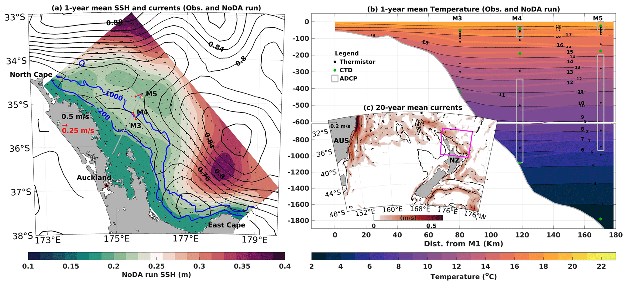
Figure 1(a) Study area showing the 1-year average SSH from AVISO (black contours) and the NoDA run (green–red shade) and the near-surface velocity NoDA run (black arrows). The stations M3 to M5 are indicated along the grey line. The coloured arrows represent the vertically averaged (bin =280 m) in situ velocities centred at 140 m (red), 420 m (cyan), 700 m (blue) and 980 m (yellow). (b) Temporal averages of temperature from in situ measurements (coloured contours) and the NoDA run (coloured shade). The grey rectangles show regions sampled by ADCPs at M4 and M5, and the vertical positions of thermistors and CTDs are indicated as black and green dots, respectively. (c) Location of the study area (magenta contour) in the southwest Pacific Ocean. The colours and arrows represent the 20-year average of geostrophic currents. Current speeds lower than 0.05 m s−1 were masked. The 200 and 1000 m isobaths are shown as blue and black contours in (a) and (c).
2.1 Numerical model
We use the Regional Ocean Modeling System (ROMS), a primitive-equation, hydrostatic and free-surface ocean model that solves the Reynolds-averaged form of the Navier–Stokes equations. ROMS is a fully nonlinear, finite-difference model that uses terrain-following (sigma) vertical coordinates and horizontal orthogonal curvilinear coordinates on a staggered Arakawa C grid (Shchepetkin and McWilliams, 2003, 2005; Haidvogel et al., 2008). The model domain (290×150) is rotated 52.14∘ clockwise to better resolve the NZNES and spans 332 km offshore at the widest point (near North Cape) (Fig. 1). The domain has a horizontal resolution of approximately 2 km, which roughly captures coastline variability and still resolves the continental shelf and slope without large computational cost. The model has 30 vertical sigma layers, and model bathymetry was interpolated from the 250 m resolution bathymetric dataset built by the National Institute of Water and Atmospheric Research (NIWA – https://niwa.co.nz/our-science/oceans/bathymetry, last access: 27 June 2023). We use a vertical discretisation scheme that increases the resolution near the surface and bottom by applying stretching function type 4 and transformation equation option 2 (Shchepetkin and McWilliams, 2005, 2009). The vertical resolution is higher at the upper 200 m (4th–30th layer). On the slope (depth <1000 m), the vertical resolution is higher than 66 m, and in the open ocean the thickest level is 233 m (3838.6 m depth). The effect of bottom friction is parameterised using a constant drag coefficient of (Lentz, 2008), and the vertical mixing of tracers and momentum is done with K-ϵ (Rodi, 1987), using the generic length scale (GLS) scheme (Umlauf and Burchard, 2003). Baroclinic modes are resolved using a time step of 180 s, while the barotropic time step is 6 s.
Model surface forcing is from the Japanese atmospheric 55-year reanalysis for driving ocean models (JRA55-do; Tsujino et al., 2018). A previous study demonstrated that JRA55-do had the highest correlation with observed winds in comparison to other atmospheric forcing datasets in the southwest Pacific (Taboada et al., 2019). Atmospheric forcing fields of wind speed, net shortwave radiation, downward longwave radiation, relative humidity, temperature, rain and pressure are provided every 3 h and are used to compute the surface fluxes of stress, heat and freshwater using the bulk flux parameterisation of Fairall et al. (2003). The model uses initial and boundary conditions of SSH, temperature, salinity and velocities from HYCOM–NCODA (Chassignet et al., 2009) versions 91.1 and 91.2, which cover the period focus of this study. Annual average discharge from several rivers are included as lateral forcing in the model. The boundary forcing is applied daily using the Chapman (1985) condition for free surface, Shchepetkin condition (Mason et al., 2010) for barotropic velocities and mixed radiation nudging (Marchesiello et al., 2001) for baroclinic velocities, temperature and salinity. A 5 d nudging coefficient is applied towards the lateral boundaries. The model aims to simulate continental shelf, slope and rise regions, including the offshore extent of the EAuC and its eddy variability. Tidal variability is not included in this study.
2.2 Observations
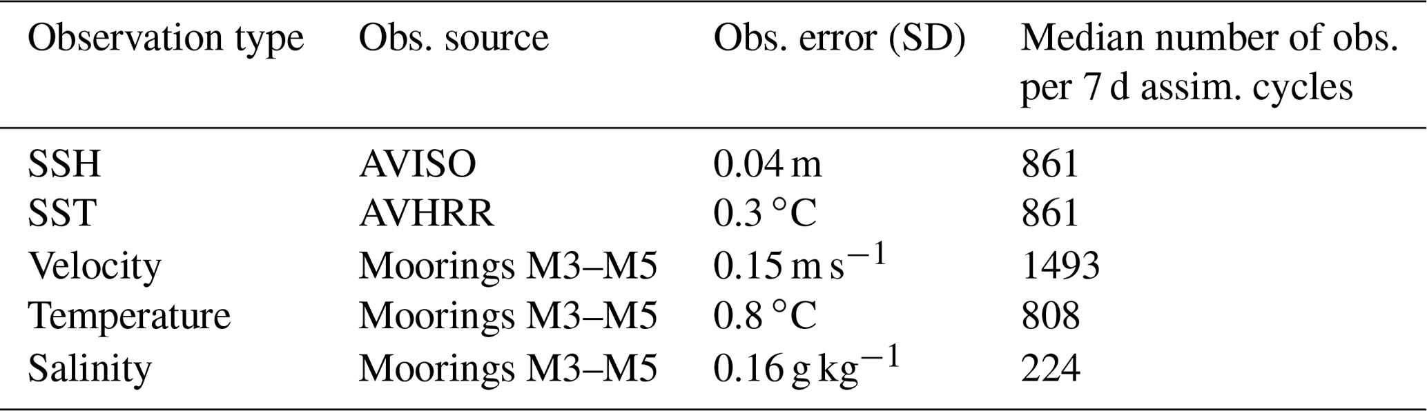
Remotely sensed observations of SSH and SST were used in all assimilative runs in this study. Optimally interpolated gridded maps of daily SSH with of horizontal resolution created by AVISO (Ducet et al., 2000) were assimilated into the model. Daily SSH offsets (annual mean of ∼51 cm) were calculated prior to every assimilation cycle as the difference between the spatial average of observations and model daily averages for each assimilative experiment (1-year averages are shown in Fig. 1a as examples of this offset). These offsets were removed from AVISO observations before assimilation to ensure the comparisons were made on the same reference surface. Daily maps of SST () from AVHRR Pathfinder (Casey et al., 2010) were used for assimilation into the model at a depth of 2 m. SSH and SST data were assimilated daily at 24:00 UTC in regions deeper than 200 m. Data points that are within 20 grid points of the boundaries were removed, and a total of 123 data points of SSH (or SST) were assimilated per day, with roughly an SSH/SST measurement every 12th grid point. We used an assimilation window of 7 d (see details in Sect. 2.3), which gives a total of 861 SSH/SST data points per assimilation cycle (Table 1).
A cross shelf–slope mooring transect collected data from 6 May 2015 to 21 May 2016 (Fig. 1a, b). In situ observations of temperature and salinity and u and v components of velocity from three moorings (M3, M4 and M5) were assimilated into the model (Fig. 1b). MicroCAT CTDs were located near the surface and bottom at the three stations, and two extra CTDs were located around 200 m at M4 and M5 (green dots in Fig. 1b). A total of 26 temperature sensors were evenly distributed between the three stations, with higher density of instruments in the upper 200 m water column (black dots in Fig. 1b). Two long-range (LR) and two short-range (SR) ADCPs were located at M4 and M5 (grey rectangles in Fig. 1b). The water column was binned every 15 m (LR) or 4 m (SR) by the upward-looking ADCPs. Velocity (temperature and salinity) measurements were taken during a period of 2 min (1 min) every 10 min or less. The dataset is freely available and can be found in O'Callaghan et al. (2015). All in situ observations were low-pass filtered at a period of 30 h to remove tidal signals and their interaction with other processes, as in Kerry et al. (2016). The observations were averaged at time bins of 6 h, centred at 03:00, 09:00, 15:00 and 21:00 UTC. Types of observations, their sources and the median number of observations per assimilation cycle are shown in Table 1.
Table 1Types of observations assimilated, their source and the median number of observations per assimilation cycle.
Independent data from 30 Argo profiles (Roemmich et al., 2019) were used for model–data-independent comparison. More details on model evaluation are described in Sect. 2.4.
2.3 Data assimilation
Data assimilation is applied in a series of time windows using strong-constraint 4D-Var, i.e. neglecting model errors (Di Lorenzo et al., 2007; Moore et al., 2011a). Tests using 2, 3, 4 and 7 d as assimilation windows were conducted, and the OSEs with a 7 d window had the most realistic results in comparison to observations. Results from a 2 d window reanalysis were also analysed in the current study. In this work, 4D-Var is used to adjust the control variables including initial, boundary and atmospheric conditions. The ocean analysis is obtained via minimisation of model-to-data discrepancy or cost function (J) given by
where δz is the state vector constituted of increments (corrections) to the initial δx(t0), lateral δb(t) and surface δf(t) conditions. D and R are the background and observation error covariance matrixes, respectively. Superscripts T and −1 represent the transpose and inverse operations, respectively.
G≡HMf, where H is the linearised version of the observation function ℋ that maps the model state to the observation time and locations. The operator Mf denotes the tangent linear operator of the model integration about the forecast (denoted by the subscript f) over the assimilation window. For the transpose, , HT maps from observation to model space, and the MT operation integrates backward in time over the assimilation window.
Gδz−d represents the mismatch between the tangent linear model fields mapped to the observations (Gδz) and the observations d, which is called the innovation vector and is defined as the difference between observations and model background interpolated to observation location. SSH observations had a daily bias (or offset) between data and model reduced from the observations before the innovation values were computed.
The combination of control variables δza that minimises J is yielded iteratively in the subspace spanned by the linear combinations of the observed model variables. The method chosen in the present work is the physical-space statistical analysis system (4D-PSAS), and the algorithm that minimises the cost function is shown in Fig. 2 in Moore et al. (2011a). 4D-PSAS defines δza as
δza can be equivalently written as δza=DGTwa, where wa is the subspace of the model state vector spanned by the observations (i.e. the dual space) and satisfies
The dual form has the advantage that the dimension of wa is equal to the number of observations, which is, in our case, several orders of magnitude smaller than the dimension of the full state vector. Thus, solving Eq. (3) may be less demanding than solving Eq. (2) (Moore et al., 2011a). In addition, the number of observations d in Eq. (2) increases with the assimilation window; therefore, it is expected that runs with longer assimilation windows (7 d) rely more on observations rather than on background terms.
In practice, we find an acceptable reduction in the model-to-data discrepancy after 20 iterations (inner loops) when atmospheric and lateral forcings are adjusted every 12 h along with initial conditions at the beginning of the assimilation cycle. For further details of the method and its application, readers are referred to Moore et al. (2011a, b).
The diagonal background/prior error covariance matrix D cannot be completely calculated or stored; it is rather estimated via factorisation (Weaver and Courtier, 2001). D takes into consideration the background error standard deviations of initial, boundary, and forcing conditions; spatial decorrelation scales; and normalisation factors (Moore et al., 2011a). The background error standard deviations were calculated from the average of 4 d variances computed from 2 years of the NoDA run ocean (initial conditions), boundary and forcing fields. Spatial decorrelation scales are implemented on D to limit the impacts of observations within certain ranges. Horizontal decorrelation length scales for SSH, velocities and active tracers (temperature and salinity) were 100, 50 and 100 km. Vertical decorrelation length scales for velocities and active tracers were 50 and 100 m. The normalisation factors are the costliest part of the covariance modelling, but they are computed only once for each combination of background error standard deviations and spatial decorrelation length scales. The normalisation factors were estimated via randomisation (Fisher and Courtier, 1995) using 7500 iterations. Figure 3 in de Paula et al. (2021) shows an example of convolution of a unit impulse function with the horizontal (vertical) decorrelation length scale set to 100 km (50 m). For more details on the computation of the background error covariance matrix D, see Moore et al. (2011a).
The observational error covariance matrix R is assumed to be diagonal. The standard deviation used was the largest value between an assigned standard deviation and the observation error obtained from the AVISO and AVHRR products, with the assigned value being the highest most of the time. This strategy was applied to satellite observations, whereas in situ data used a given standard deviation only. According to values used in the literature (e.g. Moore et al., 2011b; Kerry et al., 2016), different standard deviations were tested, and the values that gave the best results were 0.04 m for SSH, 0.3 ∘C for satellite SST, 0.8 ∘C for subsurface temperature, 0.16 g kg−1 for subsurface salinity, and 0.15 m s−1 for water column u and v components of velocities. A large standard deviation was attributed to in situ temperature due to strong internal tides in the region and blow-down events that often happened at the three moorings. Depth of the thermistors was obtained assuming an inverted pendulum relationship between CTDs located near the surface and bottom (Stanton and Morris, 2004), but a level of uncertainty remains in the depth of measurements. A summary of the observation standard deviation errors and the median number of observations per 7 d assimilation cycles is shown in Table 1.
2.4 Experiment design and evaluation metrics
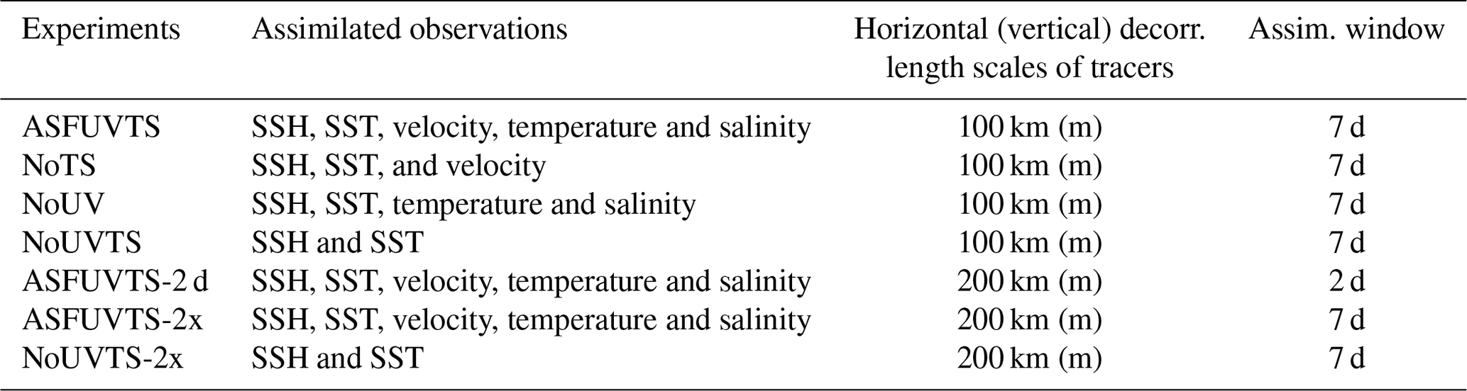
Four data assimilation experiments and one free-running simulation (no data assimilation; NoDA) are part of the OSEs. The first data assimilation experiment incorporated SSH and SST and u and v components of velocity, mooring temperature and salinity (ASFUVTS). The other data assimilative experiments were similar but withheld subsurface temperature and salinity (NoTS), subsurface velocities (NoUV), and all mooring data (NoUVTS). Another experiment assimilating surface and all mooring data was also conducted using a 2 d assimilation window (ASFUVTS-2 d), which was designed to better match the observations. This experiment (ASFUVTS-2 d) differed from the other simulations in three aspects. It used 7 d variances to compute background error standard deviations and 200 km (m) as horizontal (vertical) decorrelation length scales of active tracers (temperature and salinity). The last difference is the 2 d assimilation window, which makes increments to the initial conditions more frequent. These modifications made ASFUVTS-2 d less comparable to the rest of the OSEs, but they were needed in order to achieve the best match between assimilated and independent observations – for results, see Sect. 3.2 and 3.3. Two other 7 d assimilation window experiments (ASFUVTS-2x and NoUVTS-2x) were run assimilating the same observations as in ASFUVTS and NoUVTS but with the background error covariance matrix used in ASFUVTS-2 d (doubled decorrelation length scales and 7 d variances). Those experiments showed that using doubled decorrelation length scales of tracers can lead to larger errors in temperature if subsurface data are not available. Those experiments were needed and are recommended during the development of an ocean operational forecast. Table 2 summarises the experiments' configurations.
Table 2Assimilation experiments and their observations, decorrelation length scales of temperature and salinity, and assimilation window.
The numerical simulations started on 1 May 2015 using an initial condition interpolated from HYCOM–NCODA, and they ran until 31 May 2016. The simulations started assimilating SSH and SST observations on 1 May and mooring data between 8 May 2015 and 21 May 2016. The simulations assimilated SSH and SST until 31 May 2016, and 57 (200) assimilation cycles were performed in the 7 d (2 d) reanalyses. The NoDA run was integrated until 31 December 2016. Model results were interpolated to the observations' spatial resolution for evaluation.
The NoDA run and reanalyses were objectively validated using root mean square deviation (RMSD) given by
and linear correlation (r)
between observed (x) and modelled (y) results, where is the observation times or locations, and the averages − were applied in time or space. The daily offset between observed and modelled SSH was removed before performing the SSH RMSD calculation. SSH and SST RMSDs were computed using daily averaged model results (analysis) interpolated to observation locations inside the domain. Complex vector correlation was computed between simulated and observed 2D velocity vectors. Complex correlation converts a pair of 2D vector series into complex numbers and computes the correlation between their real parts and their relative angular displacement using their imaginary parts (Kundu, 1976). Model bias is defined as the difference between simulated and observed quantities. Statistics computed between model and in situ observations used daily averaged data processed and studied in Santana et al. (2021). A total of 30 Argo profiles were available inside the model domain (see Sect. 3.3 for details) during the reanalyses period, and these were used to provide independent temperature and salinity observations for model–data comparison. Argo data and model results were linearly interpolated from 0 to 2000 m depth using bins of 10 m. HYCOM–NCODA analyses, which assimilated SSH, SST and Argo profiles (Chassignet et al., 2009), were also compared against subsurface mooring and Argo data.
3.1 DA impact on surface fields
Documented periods with anti-cyclonic (A1 and A2) and cyclonic (C2) mesoscale eddies (Santana et al., 2021) were used to compare the NoDA and ASFUVTS runs. ASFUVTS' SSH height fields showed good agreement with observed SSH structures, where the centre of modelled high and low SSH tended to match with the core of anti-cyclonic (A1 and A2) and cyclonic (C2) eddies, respectively (Fig. 2a, c, e). The NoDA run generated anti-cyclonic and cyclonic eddies close to the observed ones; however, the eddies' centres were displaced by tens of kilometres (Fig. 2b, d, f). This result can be attributed to SSH and velocity boundary conditions from HYCOM–NCODA, which provided accurate SSH at the border and forced the generation of eddies with the correct cyclonicity albeit displaced from the observed eddies. Smaller eddies were modelled in the two simulations due to their higher resolution (∼2 km) in comparison to the observations (∼25 km) (Fig. 2c, d). Mesoscale eddies that had their centre near the domain boundary were not well simulated by either experiment, such as the cyclonic eddy centred at 34∘ S and 174∘ E on 9 October 2015 and the anticyclonic eddy centred at 36∘ S and 178∘ E on 9 April 2016 (Fig. 2a, b, e, f). A statistical analysis of the representation of mesoscale eddies (SSH and SST fields) by the numerical experiments is shown in the rest of this section.
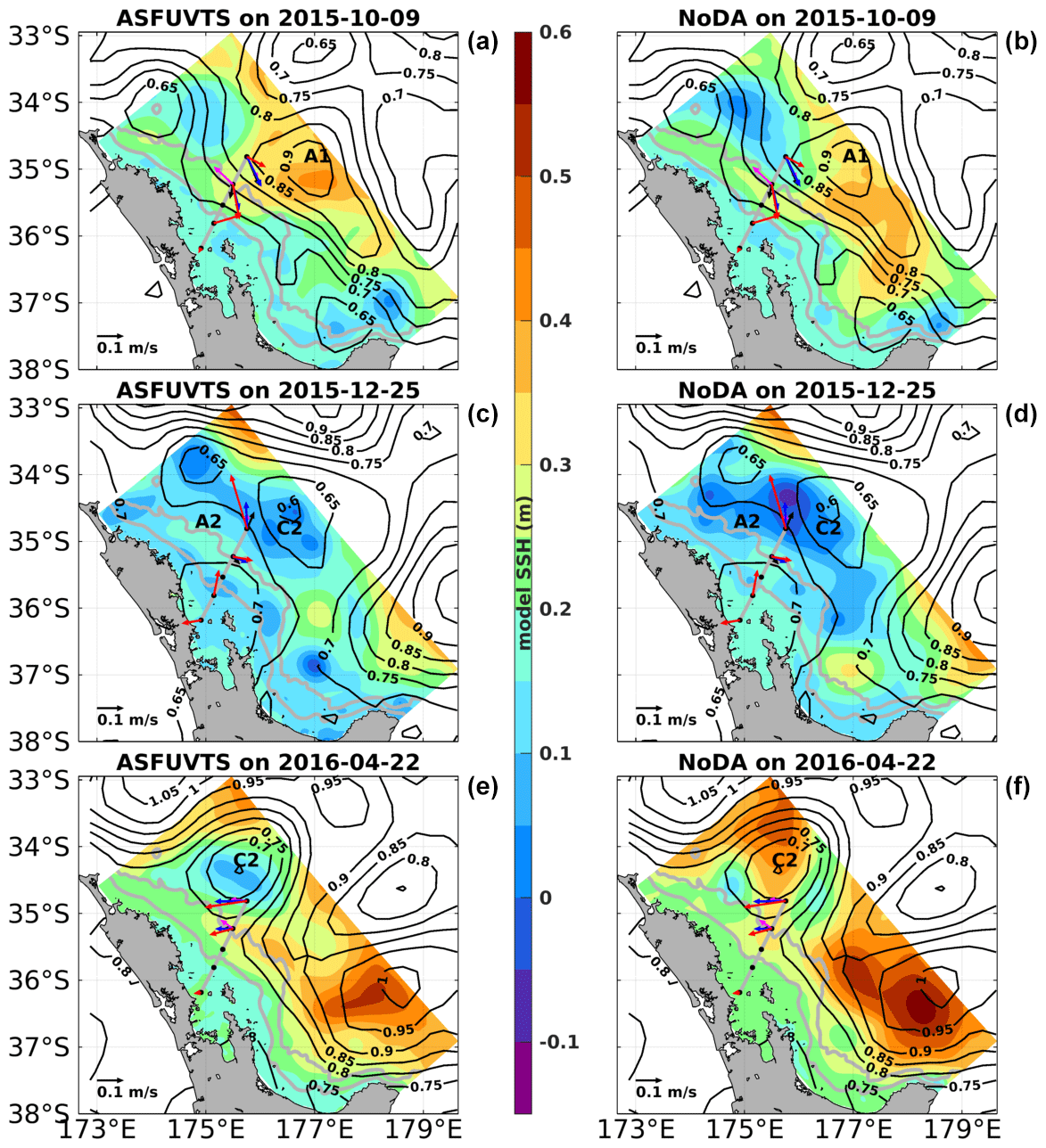
Figure 2Daily maps of observed SSH from AVISO (black contours) and modelled SSH (coloured shade) from experiments ASFUVTS (a, c, e) and NoDA (b, d, e) on the days of 9 October 2015 (a, b), 25 December 2015 (c, d) and 22 April 2016 (e, f). The abbreviations A1, A2 and C2 represent mesoscale eddies studied in Santana et al. (2021). The coloured arrows show in situ velocities as in Fig. 1a.
The RMSD was calculated in time and space against observations to objectively evaluate SSH and SST generated by the experiments. The RMSD is compared to the observations' standard deviation (SD), which shows regions or periods of larger mesoscale variability that might be harder to accurately simulate observed SSH and SST. All experiments had reduced SSH RMSD on the slope where observed SSH SD was smaller, and SSH RMSD tended to be higher in the open ocean (larger SSH SD) where mesoscale eddies are present (Fig. 3a, b, c, d). The most complete ocean analysis (ASFUVTS) had reduced SSH RMSD (mean =0.06 m) in comparison to the NoDA SSH RMSD (mean =0.08 m) for the majority of the domain (Fig. 3a, b). The NoUVTS run had similar average SSH RMSD (0.06 m) to the ASFUVTS run. However, ASFUVTS further reduced SSH RMSD upstream and downstream of the moorings (Fig. 3b, c). Experiments that assimilated in situ velocities (NoTS, ASFUVTS-2 d) also had a positive impact on SSH representation up- and downstream of the moorings (not shown). NoDA had large SSH RMSD, especially in areas of observed high SSH SD – north and east of the moorings and north of the East Cape (37∘ S, 178∘ E) (Fig. 3a, d). The dynamics in those regions were largely dominated by more than four mesoscale eddies that persisted for more than a month each (Santana et al., 2021).
The NoDA run had the highest average SST RMSD (0.72 ∘C) and showed the largest SST RMSD (4 ∘C) near the model NW boundary, which was also seen in the assimilative runs (Fig. 3f, g, h). Assimilation of surface and subsurface fields (ASFUVTS run) reduced the maximum (∼1.0 ∘C) and average (0.45 ∘C) SST RMSD values in comparison to the NoDA run (Fig. 3f, h). Withholding subsurface temperature data (NoUVTS run), as well as NoUV and NoTS runs (not shown), had small impacts on the maximum (decrease of ∼0.2 ∘C) and mean (increase of 0.01 ∘C) SST RMSDs (Fig. 3f, g).
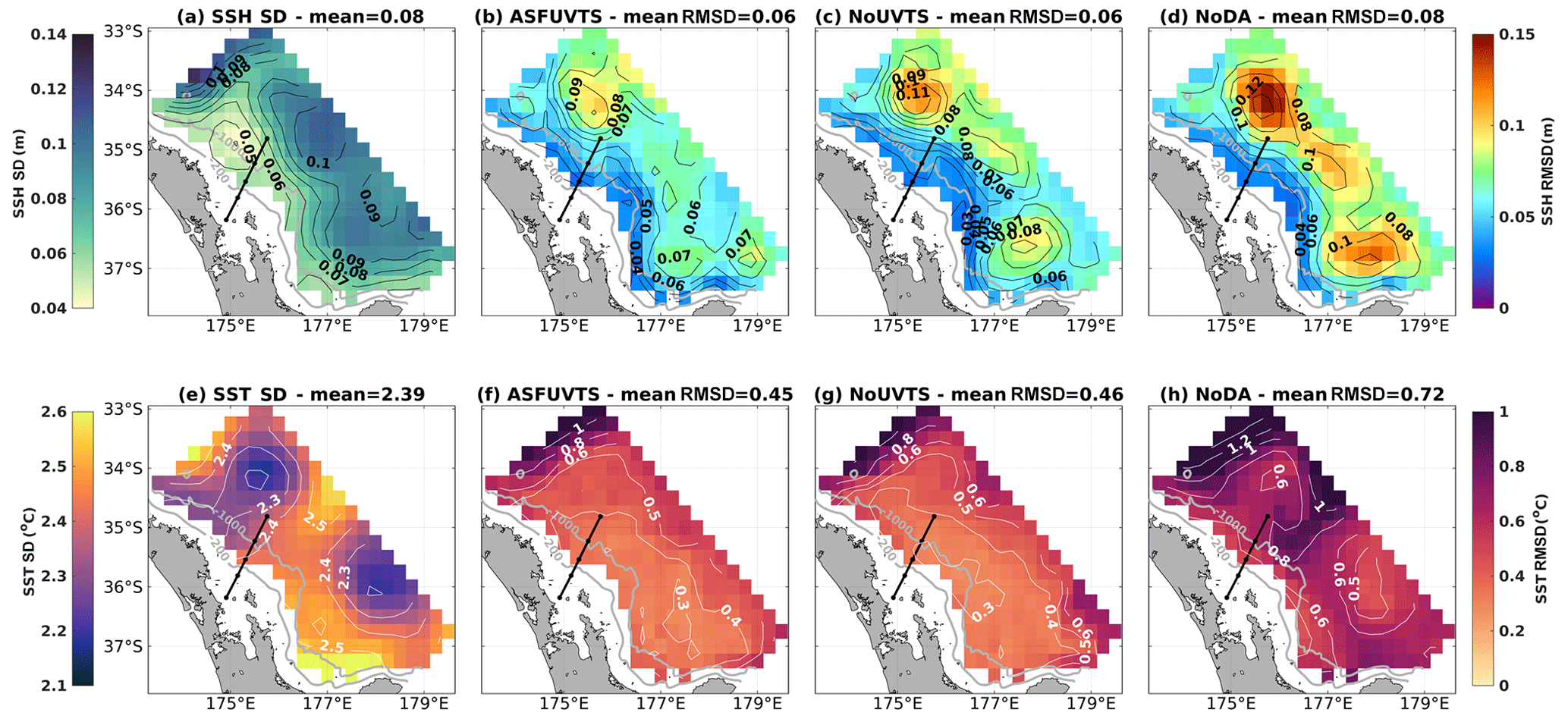
Figure 3Maps of SSH (a–d) and SST (e–h) statistics. Observed AVISO SSH SD (a) and AVHRR SST SD (e), modelled ASFUVTS run SSH (b) and SST RMSD (f), NoUVTS SSH (c) and SST RMSD (g), and NoDA SSH (d) and SST RMSD (h).
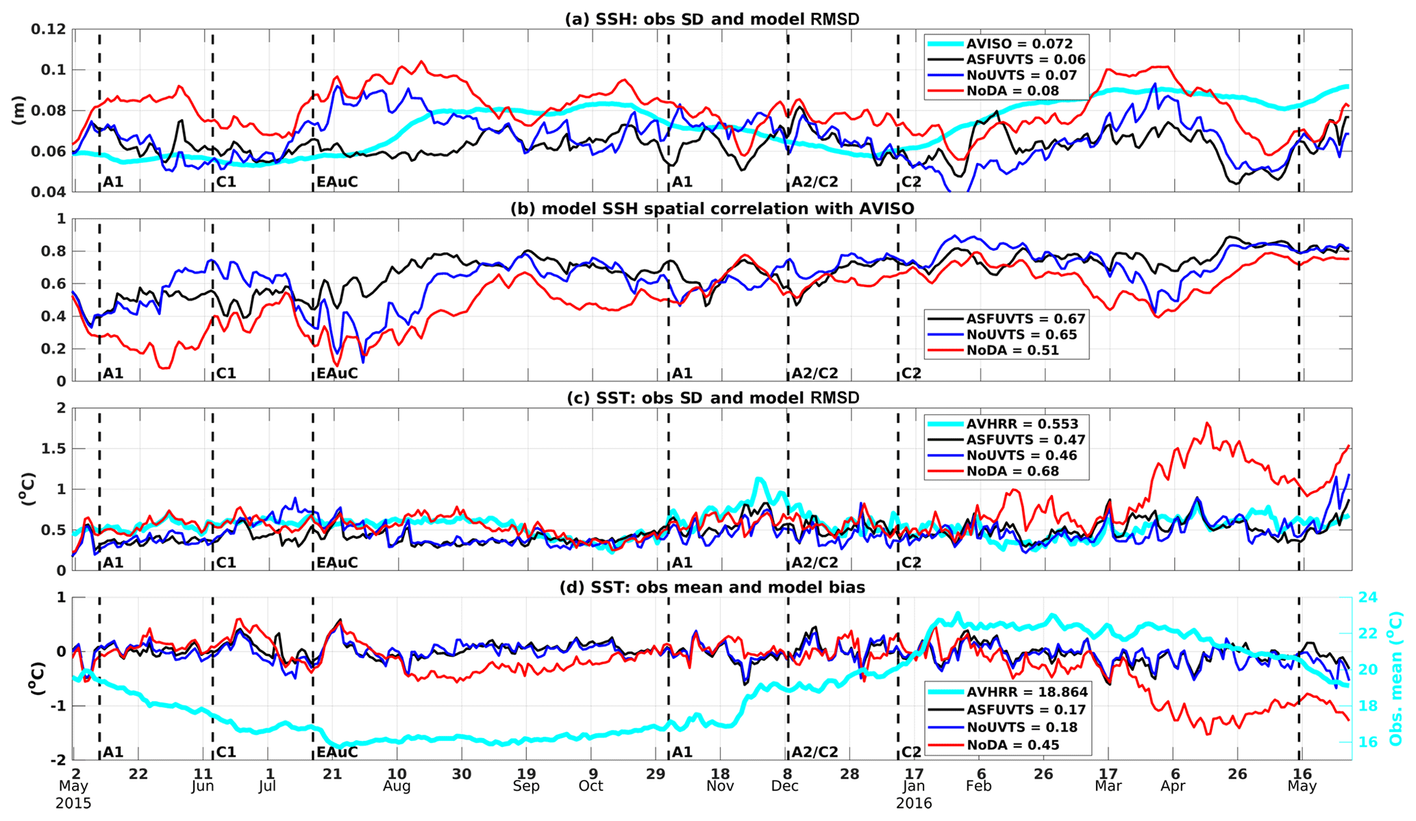
Figure 4Time series of SSH spatially observed SD and model RMSD (a), SSH spatial correlation (b), SST spatially observed SD and model RMSD (c), and SST spatial mean (right-hand axis) and model bias (left-hand axis) (d). The colours represent observations from AVISO/AVHRR (light blue) and model output from the NoDA run (red), NoUVTS run (dark blue), and ASFUVTS run (black). The mean SD, RMSD and correlation coefficients and SD SST bias are shown in the legend. The mean SST in (d) is shown in the right axis for better visualisation. The abbreviations A1, C1, EAuC, A1, A2/C2 and C2 represent mesoscale structures near M5, which were studied in Santana et al. (2021).
The NoDA run had larger spatial SSH RMSD in comparison to the ASFUVTS and NoUVTS runs for most of the year-long period of simulation (Fig. 4a). Assimilating subsurface velocity, temperature and salinity further reduced the average SSH RMSD by 14 %. The NoDA run average spatial SSH correlation was 0.51 and below 0.2 in some events (Fig. 4b). This shows the lack of skill in simulating the timing and location of the mesoscale eddies in the NoDA run. Assimilation of SSH and SST (NoUVTS) improved SSH correlation by 27 %, and the inclusion of subsurface data further increased the correlation (by 31 %), which was above 0.4 virtually during the entire year of simulation. The SSH represents the integral of subsurface density fields, which is a good proxy for representation of the whole ocean state, and the SSH was better represented when velocity, temperature and salinity observations were assimilated.
The NoDA run had spatial SST RMSD similar to the assimilative runs in the first two-thirds of the simulation period; however, it showed larger errors from February 2016 onwards and reached a maximum of 1.82 ∘C (Fig. 4c). The ASFUVTS run had smaller SST RMSD time mean (0.47 ∘C) in relation to the NoDA run (mean =0.68 ∘C). Withholding subsurface data (NoUVTS) had little impact on the SST RMSD (mean =0.46 ∘C). The NoDA run had small absolute SST difference to observations (<1.0 ∘C) during the first two-thirds of the time series, but a larger cold bias ( ∘C) was developed in April 2016 (Fig. 4d). Assimilation of surface fields only (NoUVTS) had absolute SST bias below 0.5 ∘C throughout the year-long period of simulation. The inclusion of subsurface data (ASFUVTS) did not have a well-marked impact on model SST bias; most of the surface field correction was done by assimilation of SSH and SST more specifically.
Assimilation of subsurface data (ASFUVTS) improved SST in comparison to the experiment that withheld subsurface observations (NoUVTS). A larger positive impact was shown in SSH RMSD when subsurface data were assimilated. Assimilation of in situ velocity, especially, further reduced the SSH RMSD up- and downstream of the moorings. The main differences between experiments appeared in the subsurface field comparisons, which are shown in the next section.
3.2 DA impact on subsurface fields
The NoDA run had very little velocity complex correlation (<0.1) with observations at M4 and M5 (Fig. 5a, b). DA improved complex correlation between modelled and observed velocity vectors in all experiments at the two stations. These results can be related to assimilation of SSH, which corrects the geostrophic circulation that is responsible for the long-term (>30 d) upper-half water column current variability in the region (Santana et al., 2021). The most complete assimilative run (ASFUVTS) had better results in comparison to the NoDA run but not against other assimilative runs. Withholding temperature and salinity (NoTS and NoUVTS) improved upon ASFUVTS, and NoTS had the best overall results. ASFUVTS-2 d, on the other hand, had the best overall results. HYCOM–NCODA poorly represented velocity at M4 probably due to less accurate representation of the slope bathymetry (Fig. 11 in de Souza et al., 2021). At M5, however, HYCOM–NCODA showed a velocity complex correlation coefficient similar to the 7 d assimilative runs. Velocity at M5 was more dominated by the mesoscale field and less controlled by topographic constraints when compared to M4 (Santana et al., 2021), which makes velocity easier to simulate even in lower-horizontal-resolution models.
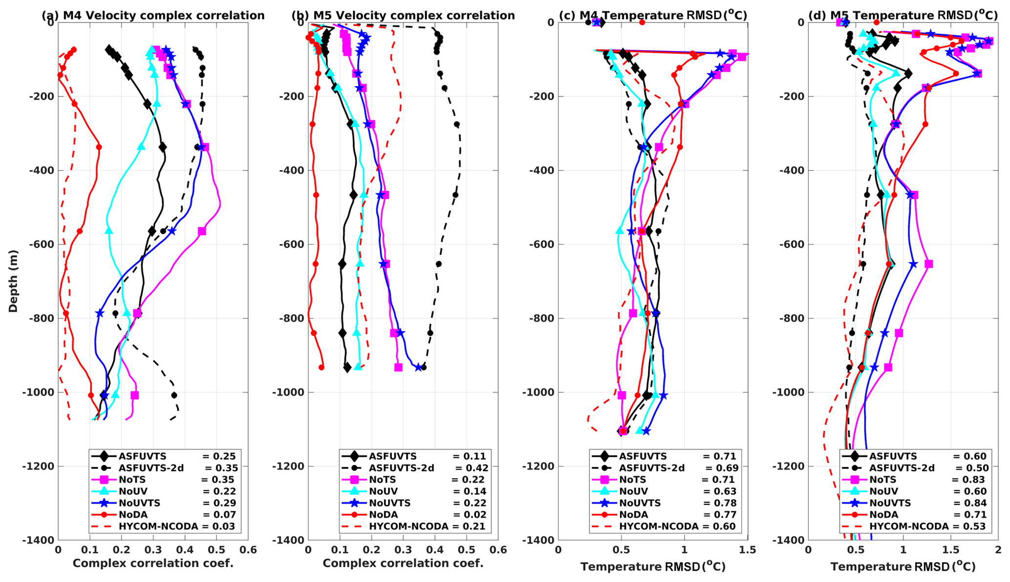
Figure 5Profiles of complex correlation coefficient between observed and modelled velocity vectors at (a) M4 and (b) M5. Profiles of temperature root mean square deviation between observed and modelled temperatures at (c) M4 and (d) M5. Black diamonds (ASFUVTS), black dots (ASFUVTS-2 d), magenta squares (NoTS), cyan triangles (NoUV), blue stars (NoUVTS) and red dots (NoDA) represent the median depth of thermistors and CTDs at each station, except at the surface where comparisons are against AVHRR SST. HYCOM–NCODA results are shown as dashed red lines. The depth-averaged values of complex correlation and temperature RMSD are shown in the legends.
The assimilative experiments had smaller temperature RMSD at the surface in comparison to the NoDA run at M4 and M5 (coloured markers at the surface in Fig. 5c, d). Assimilating subsurface temperature (ASFUVTS and NoUV) generated temperature RMSD smaller than the NoDA run RMSD in the upper 500 m at M4 and M5 (black and light blue lines in Fig. 5c, d). The lack of subsurface temperature for assimilation (NoTS and NoUVTS), however, led to larger RMSD (>1 ∘C) in the upper 200 m at M4 and M5 and below 500 m at M5 (pink and dark blue lines in Fig. 5c, d). The ASFUVTS-2 d run had improved temperature RMSD down to 1000 m at M5. HYCOM–NCODA showed improved temperature compared to the NoDA run (dashed and solid red lines in Fig. 5c, d). This is because HYCOM–NCODA assimilates temperature and salinity data from Argo floats.
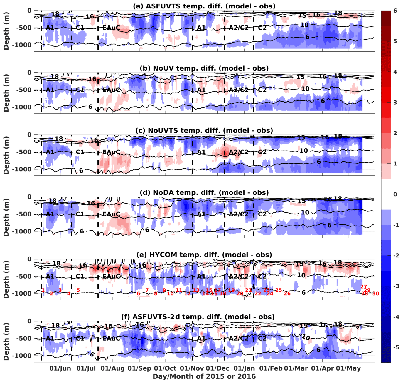
Figure 6(a) Difference between modelled and observed daily average temperature at M4 for experiments (a) ASFUVTS, (b) NoUV, (c) NoUVTS, (d) NoDA, (e) HYCOM–NCODA and (f) ASFUVTS-2 d. The red numbers in (e) show the dates when Argo profilers sampled the NZNES. The locations of the Argo floats are shown in Fig. 10e. The abbreviations A1, C1, EAuC, A1, A2/C2 and C2 represent mesoscale structures near M5, which were studied in Santana et al. (2021).
Temperature differences between models and observations at M4 showed small cold bias and relative warming at the beginning of the time series for all experiments (Fig. 6). The small biases can be attributed to the initial and boundary conditions obtained from HYCOM–NCODA analysis, which shows a relative warming between July and August 2015 when Argo data were not available in the region (red shade and numbers in Fig. 6e). Larger differences between the OSEs started to appear in September 2015. The ASFUVTS and NoUV runs are colder than observed between September and November 2015 and March and May 2016 ( ∘C – second-lightest blue shade in Fig. 6a, b). The NoUVTS and NoTS (not shown) runs are cooler in the upper 200 m water column from September 2015 onwards (Fig. 6c). Withholding subsurface temperature for assimilation (NoUVTS and NoTS) led to the continuous cooling of waters in the top 200 m until the end of the simulation. The NoDA run had a small temperature difference when compared to observations in September 2015, but these increased in October 2015 (Fig. 6d). The longest persistent cold bias in the NoDA run started in mid-March 2016, associated with the SST cold bias during the same period (Fig. 4d). Cooling of the upper water column in the NoTS and NoUVTS runs also occurred in the NoDA run. This effect might be intrinsic to the model configuration, and data assimilation of velocities and/or surface fields enhanced this bias. ASFUVTS-2 d had a marked negative temperature difference between August and September 2015 that was reduced in the rest of the year (Fig. 6e).
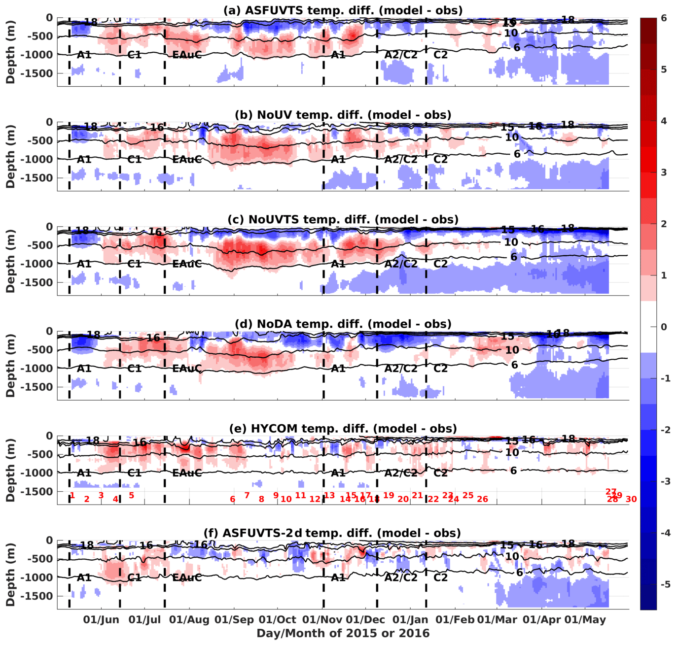
Figure 7(a) Difference between modelled and observed daily average temperature at M5 for experiments (a) ASFUVTS, (b) NoUV, (c) NoUVTS, (d) NoDA, (e) HYCOM–NCODA and (f) ASFUVTS-2 d. The red numbers in (e) show the dates when Argo profilers sampled the NZNES. The locations of the Argo floats are shown in Fig. 10e. The abbreviations A1, C1, EAuC, A1, A2/C2 and C2 represent mesoscale structures near M5, which were studied in Santana et al. (2021).
At M5, a mid-water-column warm bias (>1 ∘C) was simulated in the first half of the year-long period in all OSEs (second-lightest red shade in Fig. 7a, b, c, d). This also appeared in HYCOM–NCODA between June and September 2015 (Fig. 7e) probably due to the lack of Argo floats to the north of 35∘ S. ASFUVTS had the smallest differences to the observations out of all 7 d assimilation window experiments (Fig. 7a). In mid-August 2015, a near-surface cold bias ( ∘C) was pronounced in all experiments but was further developed in the NoDA, NoTS and NoUVTS runs towards the end of the simulation period. This is associated with the lack of subsurface temperature and the near-surface cold bias in the NoDA run. The ASFUVTS (NoUV) run reduced the cold (warm) differences to values above −1 ∘C (below 2 ∘C) for most of the period of the simulation. It showed that the assimilation of subsurface temperature and salinity had a positive impact by reducing temperature biases at M4 and M5. ASFUVTS-2 d better matched the observations and had the smallest temperature differences at M5 (Fig. 7f). However, this assimilation configuration led to larger temperature differences when mooring temperature was not assimilated. Consequently, this configuration is not advisable in this region for an operational forecast system, as Argo floats can spend months without sampling the region.
Observed salinity time series from CTDs located near 200 m depth at M4 and M5 were compared to simulated salinity from three experiments and HYCOM–NCODA (Fig. 8). All models' salinity tended to oscillate near the observed values, and average absolute biases were smaller than 0.1 g kg−1. The ASFUVTS run slightly degraded salinity results in comparison to the NoDA run; however, salinity RMSDs were smaller than the observation standard deviation (0.16 g kg−1). ASFUVTS-2 d and HYCOM–NCODA had larger peaks and troughs in salinity time series and the largest variances (0.02 g kg−1) at M5. This result can be attributed to the frequency of increments applied to the initial conditions – everyday in HYCOM–NCODA and every other day in ASFUVTS-2 d. Despite that, ASFUVTS-2 d had the best statistical performance amongst the simulations, which can also be attributed to the more frequent corrections to the initial conditions.
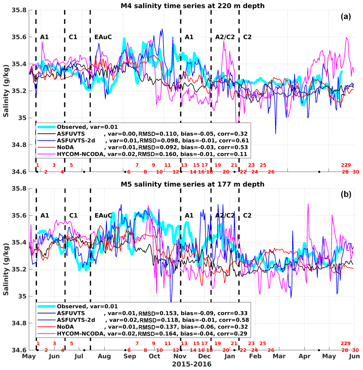
Figure 8Observed (light blue) and modelled daily average salinity near 200 m depth at M4 (a) and M5 (b) from experiments ASFUVTS (black), ASFUVTS-2 d (dark blue), NoDA (red) and HYCOM–NCODA (magenta/pink). Some experiments had their colour changed from previous plots for better visualisation. Var, RMSD, bias and corr represent variance, root mean square deviation, mean bias and correlation coefficient calculated between modelled and observed salinity. The red numbers show the dates when Argo profilers sampled the NZNES, and their locations are shown in Fig. 10e. The abbreviations A1, C1, EAuC, A1, A2/C2 and C2 represent mesoscale structures near M5, which were studied in Santana et al. (2021).
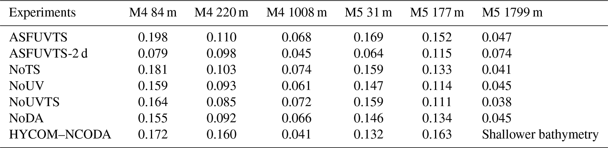
Salinity RMSD comparisons at three different depths at M4 and M5 are shown for all ROMS experiments and HYCOM–NCODA in Table 3. These experiments had salinity RMSDs oscillating around 0.16±0.04 g kg−1 in shallower depths (≤220 m) at M4 and M5 stations. An exception to this is ASFUVTS-2 d, which had the smallest salinity RMSD (<0.10 g kg−1) in the upper M4 and M5 depths. HYCOM–NCODA also had salinity RMSD around 0.16±0.04 g kg−1 in the upper and 200 m depth at both M4 and M5. Salinity RMSD was reduced near the bottom at M4 and M5 (<0.08 g kg−1) in all ROMS experiments as well as for HYCOM–NCODA. ASFUVTS-2 d, however, had the largest salinity RMSD near the bottom at M5. The bathymetry used in HYCOM–NCODA was shallower than near-bottom measurements at M5, and salinity RMSD was not calculated. These OSE's results suggest that future experiments should reduce salinity observation standard deviation (or error) below a certain depth. For instance, observed salinity error can be reduced to 0.06 g kg−1 below 1000 m as in Kerry et al. (2016), or an exponential decay can be applied from the surface (0.12 g kg−1) to 2000 m (0.02 g kg−1) (Xie and Zhu, 2010; Mignac et al., 2015; Santana et al., 2020). In the next section, model temperature and salinity are validated against Argo-independent observations.
Table 3Salinity root mean square deviation (RMSD) between experiments and CTD observations at M4 and M5.
3.3 Comparison to independent observations
A total of 30 non-assimilated temperature and salinity profiles spread in time (Fig. 9) and throughout the domain (Fig. 10e) were used for independent comparison. All experiments had small salinity differences when compared to the first five salinity profiles sampled by Argo floats, which can be attributed to HYCOM–NCODA's initial and boundary conditions (Fig. 9). Larger salinity differences, however, appeared in the OSE's results in late August when simulated sea water was fresher in the upper 200 m depth and saltier underneath. Assimilation of surface and mooring data using a 7 d window did not generate any notable positive/negative impact in salinity in comparison to the NoDA run. ASFUVTS-2 d had the smallest differences between simulated and observed salinity (Fig. 9f), and its results were similar to HYCOM–NCODA (Fig. 9e), which assimilates Argo data. However, fresher sea water was simulated in mid-May 2016 when mooring salinity data collection had ended.
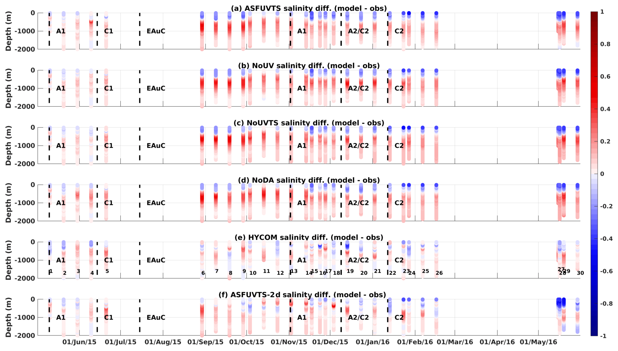
Figure 9Salinity difference between modelled and Argo observations from experiments (a) ASFUVTS, (b) NoUV, (c) NoUVTS, (d) NoDA, (e) HYCOM–NCODA and (f) ASFUVTS-2 d. The numbers in (e) show the dates when Argo profilers sampled the NZNES. The locations of the Argo floats are shown in Fig. 10e. The abbreviations A1, C1, EAuC, A1, A2/C2 and C2 represent mesoscale structures near M5, which were studied in Santana et al. (2021).
In this analysis, we included experiments using a 7 d assimilation window and doubled decorrelation length scales for tracers (NoUVTS-2x and ASFUVTS-2x) to show the impact of the larger decorrelation length scale on simulating temperature and salinity at Argo locations. All experiments' temperature RMSDs showed similar patterns to the results simulated at M4 and M5. When temperature was not assimilated (NoUVTS and NoTS), there was a higher temperature RMSD between 0 and 200 m in comparison to the NoDA run due to a colder bias ( ∘C) that developed in these runs (Fig. 10a, b). Assimilation of subsurface temperature data (ASFUVTS, ASFUVTS-2 d and NoUV runs) resulted in smaller temperature RMSD in comparison to the NoDA run from the near surface down to 2000 m (Fig. 10a, b). HYCOM–NCODA reanalysis, which assimilates Argo, SSH and SST data, had the overall best temperature representation at the Argo locations. Assimilation of surface and mooring data using doubled decorrelation length scales (ASFUVTS-2x) slightly improved temperature representation near the surface and around 1000 m depth in comparison to ASFUVTS (Fig. 10a, b). However, when subsurface data were not assimilated (NoUVTS-2x), larger temperature RMSDs were generated between 200 and 1200 m depth in relation to the NoUVTS run.
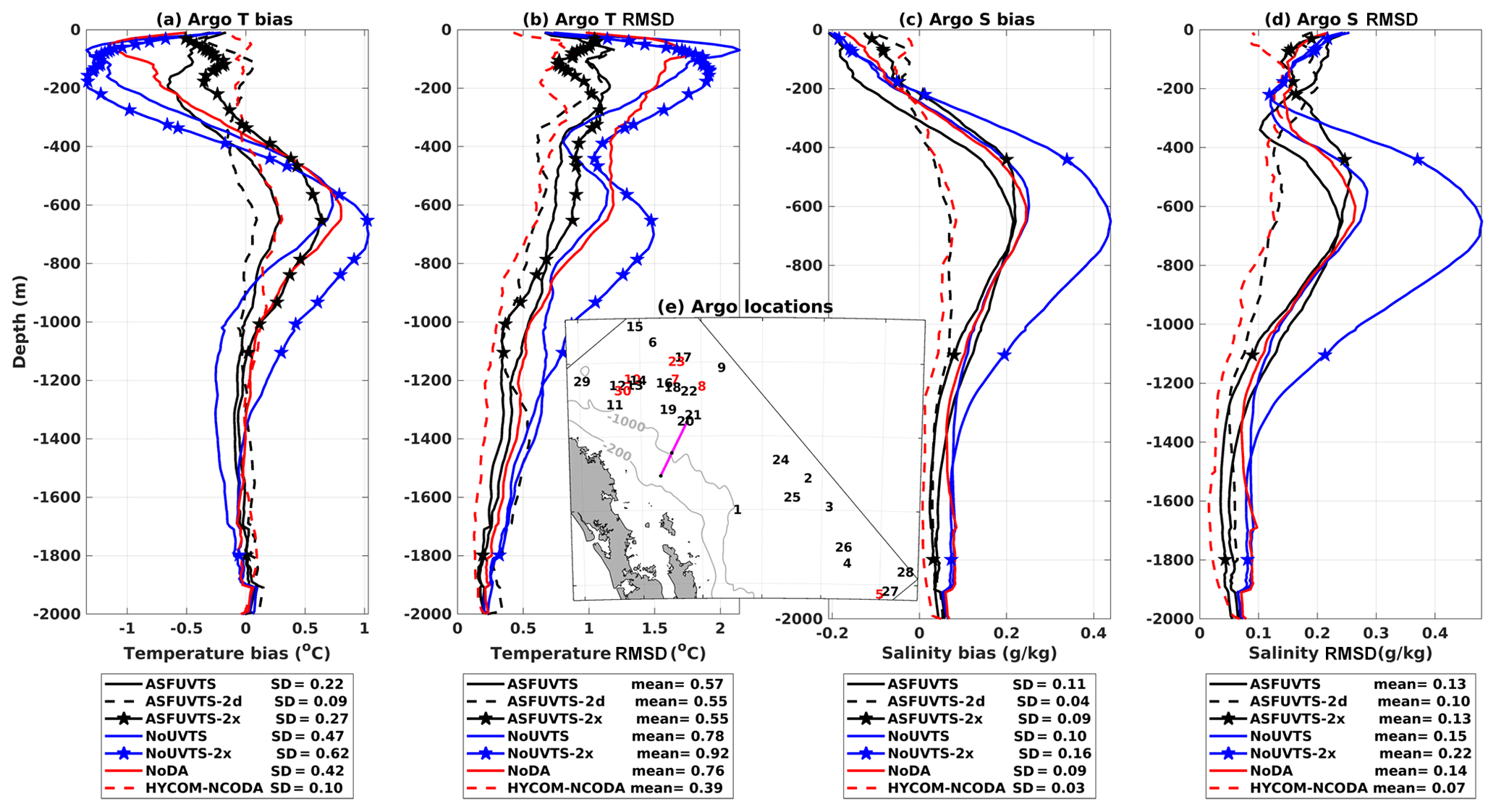
Figure 10Profiles of mean bias and root mean square deviation (RMSD) between model and independent Argo observations of temperature (a, b) and salinity (c, d). Solid black line (ASFUVTS), dashed black line (ASFUVTS-2 d), starred black line (ASFUVTS-2x), solid blue line (NoUVTS), starred blue line (NoUVTS-2x), red line (NoDA), and dashed red line (HYCOM–NCODA). The stars represent the median depth of thermistors and CTDs (CTDs) at M3, M4 and M5 in temperature (salinity) bias and RMSD profiles. Results from experiments NoUV and NoTS were not shown for better visualisation. (e) Map of Argo locations, which are represented as numbers in black or red for better visualisation only. The moorings' locations are shown as black dots on the magenta line.
Comparisons to Argo salinity measurements showed that all 7 d window experiments and the NoDA run had similar vertical structures in the salinity bias. Fresher salinity was modelled in the upper 200 m, and saltier waters were modelled below that, peaking at 600 m, in these experiments (Fig. 10c). ASFUVTS-2 d had the smallest salinity bias and RMSD in comparison to the 7 d window experiments (Fig. 10d). This suggests that more frequent corrections/increments to the initial conditions and doubled decorrelation length scales of tracers can improve salinity even with the small number of salinity observations. The ASFUVTS-2 d salinity results were close to HYCOM–NCODA reanalysis, which assimilated salinity data from Argo floats.
Applying doubled decorrelation length scales of tracers to the 7 d assimilation window experiments slightly reduced RMSD for temperature (3 %) and salinity (4 %) at the Argo locations when assimilating mooring temperature and salinity (ASFUVTS-2x) in comparison to using 100 km (100 m) as horizontal (vertical) length scale (Fig. 10). However, when subsurface data were withheld (NoUVTS-2x), it increased the mean temperature (salinity) RMSD by 18 % (47 %). Larger RMSD occurred when withholding mooring temperature and salinity data using a 2 d assimilation window and double decorrelation length scales of tracers (NoUVTS-2 d – not shown).
3.4 Increments to initial and surface conditions
Variability in temperature increments to the initial conditions at M4 revealed oscillation between positive and negative increments through time in all experiments (Fig. 11). The 7 d window experiments that assimilated subsurface temperature and salinity (ASFUVTS and NoUV) had positive increments extending from the surface down to 500 m (darker red shade in Fig. 11a, b). In contrast, experiments that did not assimilate temperature and salinity (NoTS and NoUVTS) had strong positive increments bounded to near the surface (Fig. 11c, d). ASFUVTS-2 d did not have large positive increments near the surface, but increments tended to vary from positive to negative values between assimilation cycles (Fig. 11e).
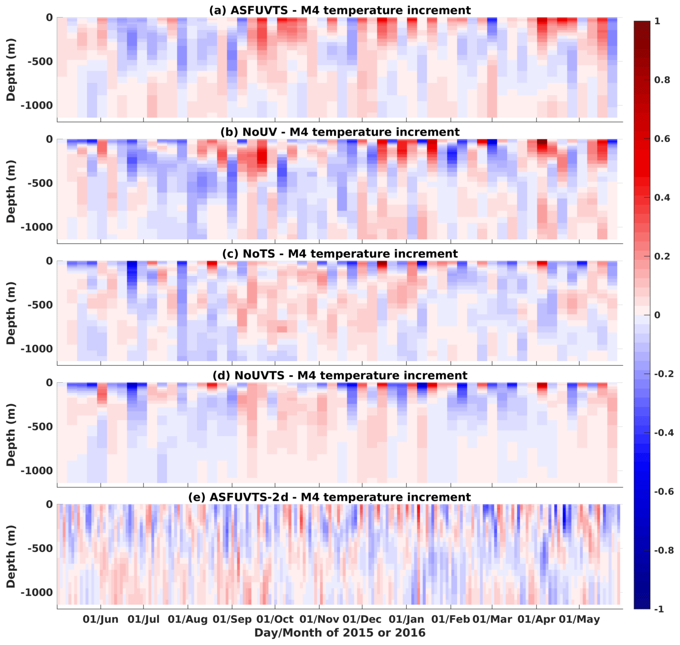
Figure 11Time variability in temperature increments (∘C) to the initial conditions at M4 from experiments (a) ASFUVTS, (b) NoUV run, (c) NoTS, (d) NoUVTS and (e) ASFUVTS-2 d.
Near-surface average temperature increments had a distinct difference between experiments that did and did not assimilate subsurface temperature at M4 and M5 (Fig. 12a, b). Assimilation of in situ temperature (ASFUVTS and NoUV) generated larger average positive increments (>0.04 ∘C) around 100 m depth in comparison to the simulations that withheld subsurface temperature (NoTS and NoUVTS). The latter experiments had near-surface mean negative temperature increments that increased towards 0 ∘C below 200 m. ASFUVTS-2 d had smaller average and standard deviation increments near the surface in comparison to the 7-day experiments (Fig. 12a, b).
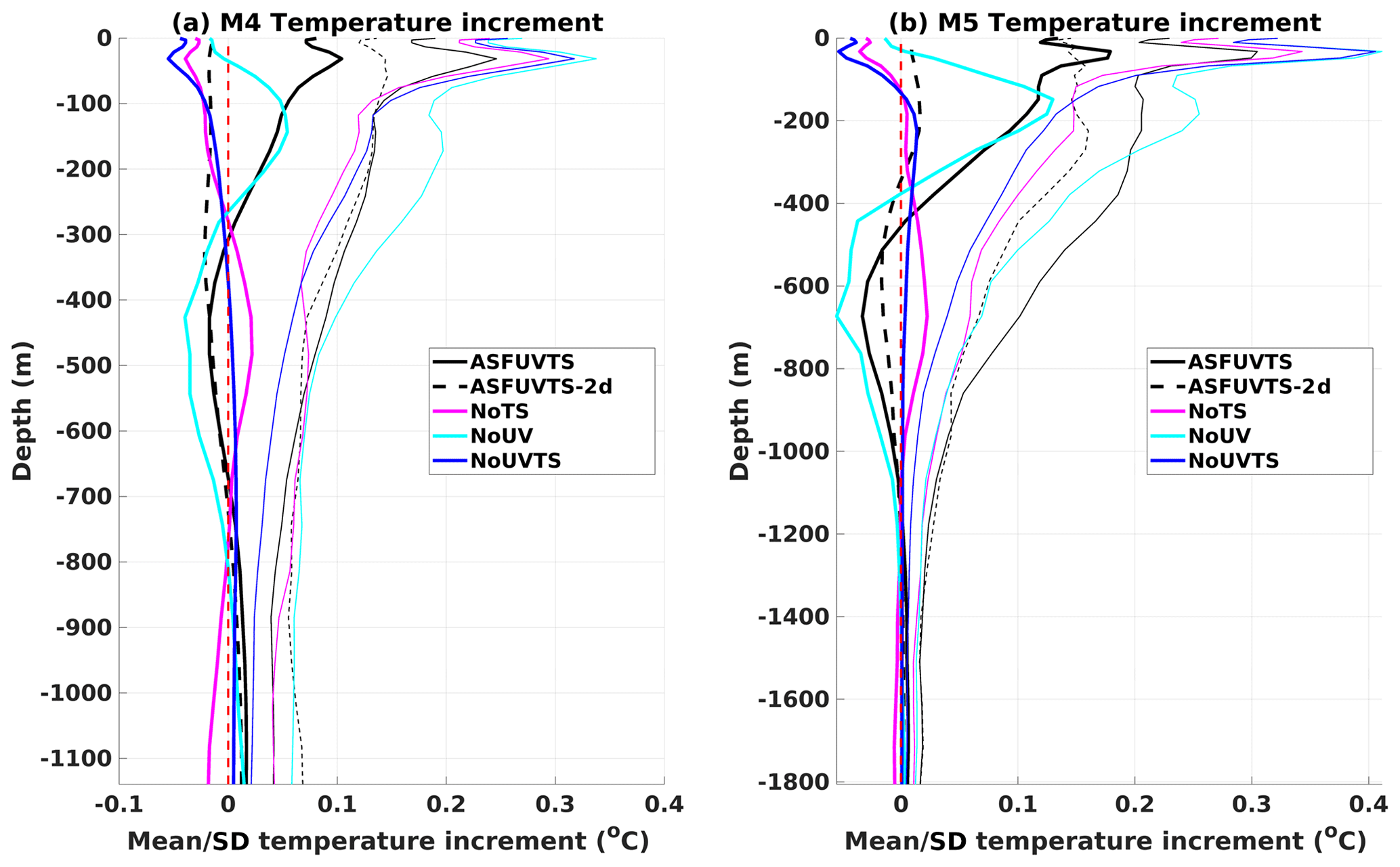
Figure 12Profile of average (thick lines) and standard deviation (thin lines) increments to initial conditions of temperature at M4 (a) and M5 (b). Solid black line (ASFUVTS), dashed black line (ASFUVTS-2 d), pink (magenta) line (NoTS), light blue (cyan) line (NoUV) and dark blue line (NoUVTS). The dashed red line marks the 0 ∘C increment.
Surface mean heat flux analysis fields varied according to the presence/absence of subsurface temperature for assimilation (Fig. 13). Simulations that withheld subsurface temperature (NoUVTS and NoTS) had large positive heat flux near the moorings and in the majority of the domain (Fig. 13a, b). The positive heat flux in the NoTS and NoUVTS runs was related to the near-surface negative temperature increments at M4 and M5 (dark blue and pink lines in Fig. 12). The combined positive heat flux and negative temperature increments corrected the surface cold bias present in the NoDA run but not the cooling trend around 200 m. Experiments that assimilated subsurface temperature (ASFUVTS, NoUV and ASFUVTS-2 d) had negative average heat flux (or near-zero heat flux – ASFUVTS-2 d) near the moorings that extended north and south with varying size between experiments (Fig. 13c, d, e). This negative heat flux increment balances the positive temperature increment at M4 and M5, which aims at correcting both surface and upper thermocline (∼200 m) cold biases. The large variability in heat flux analysis fields between experiments (Fig. 13) might be related to the 4 d variances used to compute the background error covariance. The 4 d variances used here include daily cycle and cloud coverage variabilities, which generated large heat flux uncertainty and increments.
The ASFUVTS-2 d run had smaller negative heat flux analysis near the moorings. This happened due to the smaller average negative increments (M4) and positive increments (M5) added to the initial condition of temperature at these stations (dashed black line Fig. 12). The NoDA run average net heat flux was mostly positive north of 35∘ S and was negative southwards (Fig. 13f). On average, the atmosphere has a warming effect on the ocean north of 35∘ S and a cooling effect south of 35∘ S. This is observed in JRA55-do (Fig. 48 in Tsujino et al., 2018), in which the NZNES is located near the average zero net heat flux contour line in the atmospheric forcing dataset.
Annual average wind stress is mainly from the northwest in the 7 d window runs and from the west in the ASFUVTS-2 d and NoDA runs (vectors in Fig. 14). Wind stress curl showed some spatial variability between the assimilative runs (red and green shade in Fig. 14). Experiments that did not assimilate subsurface temperature and salinity (NoUVTS and NoUV) had average negative wind stress curl at the moorings' location (Fig. 14a, b). Conversely, assimilation of subsurface temperature and salinity (NoUV and ASFUVTS) generated average positive wind stress curl on top of M5 (M3–M5 in ASFUVTS) (Fig. 14c, d). Positive wind stress curl generates convergence and downwelling of warmer water masses that might be acting to prevent the cold bias in the numerical model. These changes in wind stress curl can also explain why assimilation of subsurface temperature and salinity (ASFUVTS and NoUV) slightly degraded the representation of velocity at M4 and M5 compared to withholding subsurface temperature and salinity (NoTS and NoUVTS). The ASFUVTS-2 d run had smaller wind stress curl magnitude compared to the other simulations. Its wind stress curl field resembles the NoDA wind field forced with JRA55-do, especially in the regions of negative wind stress curl near the coast around 37.5∘ S and observed by Taboada et al. (2019) using the Cross-Calibrated Multi-Platform wind vector analysis (CCMP).
In this study, SSH, SST, mooring velocity, temperature and salinity observations were assimilated into an ocean model of the EAuC using 4D-Var with a 7 d assimilation window. Observing system experiments (OSEs) were conducted in order to elucidate the importance of in situ data assimilation in the EAuC region. Four OSEs were performed based on the most complete simulation called ASFUVTS, which assimilated surface fields (SSH and SST), mooring velocity, temperature and salinity. The other experiments withheld observation types from assimilation. They removed mooring velocities (NoUV), subsurface temperature and salinity (NoTS), and all mooring data (NoUVTS). A non-assimilative simulation (NoDA) was used as the control run. Argo data were left out for independent model–data comparison. Another run that assimilated surface and mooring data using a 2 d window (ASFUVTS-2 d) and aimed at better matching the observations rather than serving as a basis for an operational forecast was also evaluated. HYCOM–NCODA outputs, which provided boundary conditions, were also used in the model comparison.
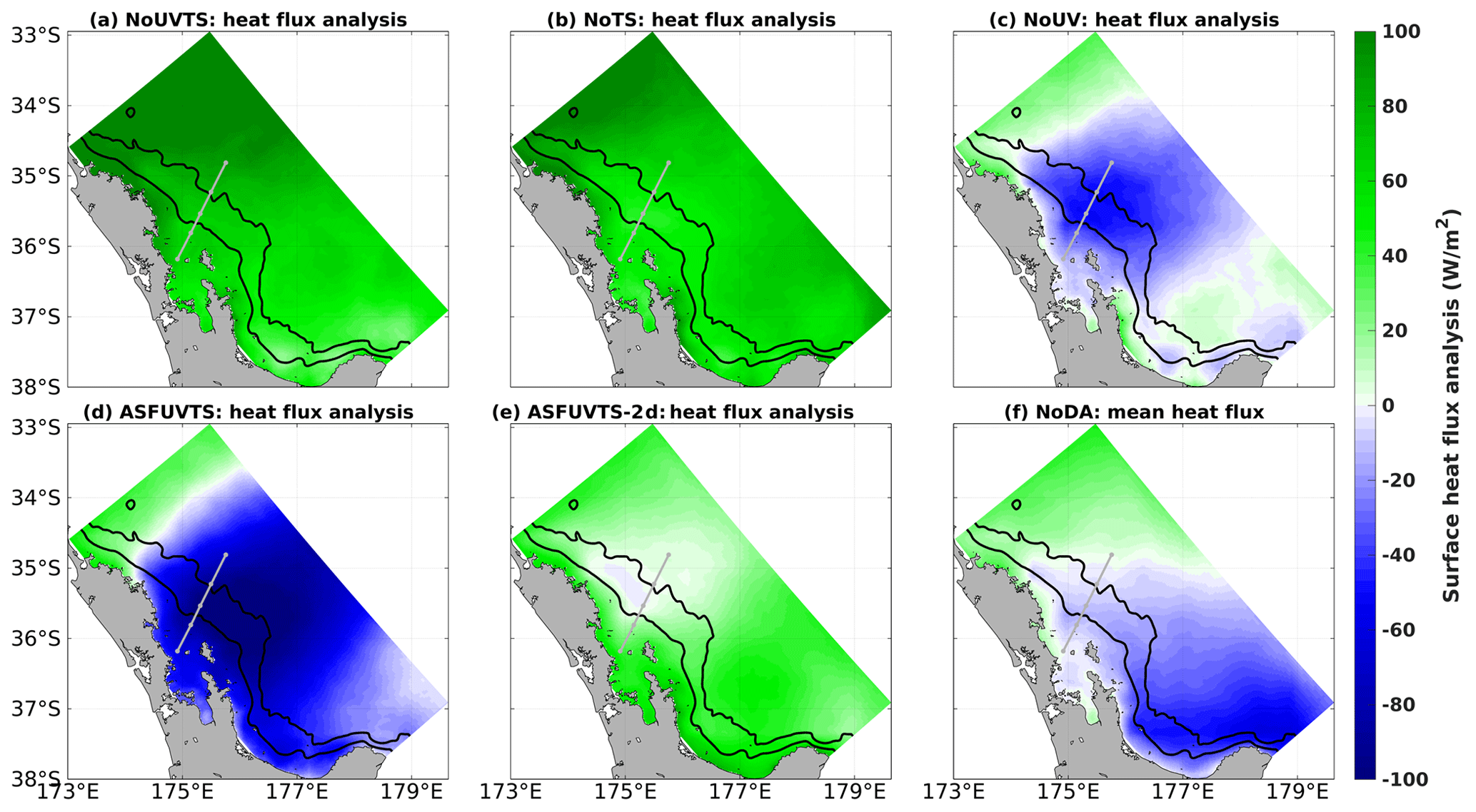
Figure 13Average surface net heat flux analysis (W m−2) (positive = downward) in experiments (a) NoUVTS, (b) NoTS, (c) NoUV, (d) ASFUVTS and (e) ASFUVTS-2 d. Panel (f) shows mean net heat flux in the freely evolving simulation (NoDA). Green (blue) colours show positive (negative) mean surface heat flux.
All assimilative experiments showed a reduction in SSH RMSD in comparison to the NoDA run of about 25 %. The improvements in SSH were small in comparison to achievements seen in other WBC 4D-Var studies, such as the East Australian Current (EAC) (∼63 % – Kerry et al., 2016) and the Brazil Current (BC) (48 % – de Paula et al., 2021). There was a smaller correction in SST (RMSD reduction of 37 %) when compared to 4D-Var studies in the East Australian Current (EAC) (∼60 % – Kerry et al., 2016) and the Brazil Current (BC) (27 % – de Paula et al., 2021). These studies used lower horizontal resolution in the open ocean (5 km in the EAC and 9 km in the BC) compared to our model spatial grid spacing (2 km), which might explain the differences in performance. According to Sandery and Sakov (2017), increasing model resolution towards the submesocale (from 10 to 2.5 km) reduces the skill of the analysis and forecast. They suggested that resolving the less predictable submesoscale lowers the predictability of the mesoscale, as there is an inverse cascade in the kinetic energy spectrum. Kerry et al. (2020) found larger errors when downscaling from a regional to a coastal domain (750–1000 m resolution) while simulating the cyclonic inshore side and frontal instabilities of the EAC.
All OSEs improved velocity complex correlation by at least three times at M4 and five times at M5 in comparison to the NoDA run (coef. <0.07). Assimilation of subsurface velocity (NoTS) simulated flow reversals at depth on the slope (M4) more accurately, and it improved on the simulation that assimilated only surface fields (NoUVTS). Counterintuitively, inclusion of temperature and salinity in the 7 d window runs (NoUV and ASFUVTS) degraded the velocity results in comparison to the NoUVTS run. This might be associated with increased positive wind stress curl near the moorings in experiments that assimilated subsurface temperature (ASFUVTS and NoUV runs). Positive wind stress curl causes downwelling of warmer waters and counterbalances the cold bias in the model but degrades velocity results in ASFUVTS and NoUV runs. The wind impact can be reduced by decreasing the number of days to estimate wind variance (uncertainty). Another factor that may have played a role was the low vertical resolution of salinity sensors, which was not enough to correct density fields and generate accurate geostrophic currents. For future data collection strategies, we suggest that higher vertical resolution for salinity data be used. The application of doubled decorrelation length scales of tracers improved temperature, salinity and velocity simulation when subsurface data were assimilated (ASFUVTS-2x and ASFUVTS-2 d). However, this strategy led to larger temperature and salinity errors when subsurface tracer data were not assimilated (NoUVTS-2x and NoUVTS-2 d).
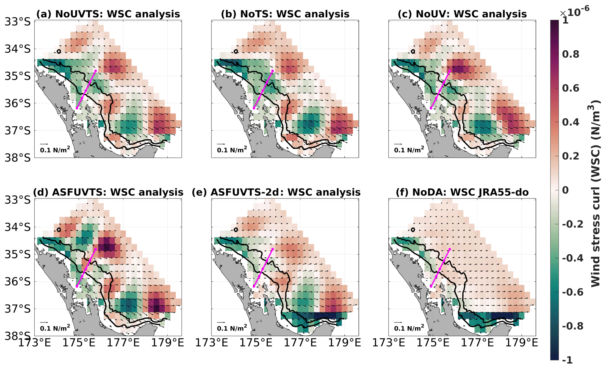
Figure 14Analysis field of wind stress (N m−2) and its curl (N m−3) (red–green shade) in experiments (a) NoUVTS, (b) NoTS, (c) NoUV, (d) ASFUVTS and (e) ASFUVTS-2 d. Panel (f) shows mean wind stress and its curl from JRA55-do. All fields were degraded from 2 km to to be similar to JRA55-do horizontal resolution.
The 2 d assimilation window run (ASFUVTS-2 d) had the highest complex correlation coefficients (>0.35) from a combination of doubled decorrelation length scales, larger model error estimates and more frequent increments. ASFUVTS-2 d was more efficient at extracting and spreading mooring observational information and generated the best results when compared to temperature and salinity from Argo observations. This ocean reanalysis can be used to estimate EAuC heat and volume transports, since it better represents observations. However, this approach should not be used if subsurface data availability is low because a large subsurface cold bias can be generated. This is the case for an operational forecast in which Argo floats might not be available for months. In Kerry et al. (2016), higher-velocity complex correlation coefficients (∼1) were obtained in a 2-year reanalysis of the EAC. However, the EAC has a more coherent jet (Mata et al., 2000; Bowen et al., 2005; Sloyan et al., 2016), which is well represented by the non-assimilative run (complex correlation ∼0.8 in some locations) (Kerry et al., 2016). In contrast, the EAuC has a more eddy-dominated field ( of 1 year) (Santana et al., 2021), which makes it harder for ocean free-running models and reanalyses to capture such variabilities.
Marked differences among the experiments appeared in the subsurface temperature. Experiments that withheld in situ temperature and salinity (NoTS and NoUVTS) generated a larger cold bias around 100 m at M4 and M5 in comparison to the NoDA run. At 100 m, RMSD was about 1.4 ∘C (1.9 ∘C) in the NoTS (NoUVTS) run at M4 and M5, whereas the NoDA run had a temperature RMSD of 1.1 ∘C (1.6 ∘C) at M4 (M5). Assimilation of in situ temperature and salinity (ASFUVTS and NoUV) reduced the cold bias. The lack of subsurface temperature assimilation also generated similar errors at the top of the thermocline in other regional studies (e.g. Zavala-Garay et al., 2012; Santana et al., 2020). Zavala-Garay et al. (2012) needed to assimilate XBT or synthetic CTD data to correct that large temperature RMSD (∼2 ∘C) between 200 and 500 m depth. The authors aimed at simulating the EAC variability between the years 2001 and 2002, and the Argo project was still in its beginning stages, with few sondes in the ocean. In our study, it is still an open question if assimilating the few Argo temperature and salinity profiles (30) and surface data would prevent the growth of the 100 m cold bias at M4 and M5. These experiments represent a good benchmark to assess proper assimilation windows and decorrelation length scales. Doubled length scales of tracers (200 km and 200 m) and a 2 d assimilation window led to colder biases in the experiments that withheld in situ temperature, which could be a problem when Argo data are not available for a long period. The 7 d assimilation window and smaller length scales (100 km and 100 m) seemed to be a good configuration to represent the surface (SSH and SST) and subsurface velocity fields well in an operational forecast system.
In ROMS 4D-Var, spatial decorrelation length scales are set using one value per model variable for the whole domain (Moore et al., 2011a). In reality, decorrelation length scales can vary in space depending on the main drivers of variability in each specific region. For instance, atmospheric heat flux dominates temperature variability at the surface, and SST at M4 has high correlation (>0.7) with points spread hundreds of kilometres across in the NoDA run (Fig. 15a). Nonetheless, this correlation is limited to a few metres below the surface (<20 m) (Fig. 15b). At 200 m depth, the high-correlation area covers a region spanning ∼50 km across and ∼350 m at depth (Fig. 15c, d). In this study, we showed that using 100 km (m) as horizontal (vertical) decorrelation length scales of tracers is a good approach to improve upon the non-assimilative (NoDA) run while preventing the degradation of subsurface temperature fields when water column data are not assimilated. However, more tests can be done while assimilating Argo data, and a non-trivial implementation of spatially variable decorrelation length scales is encouraged.
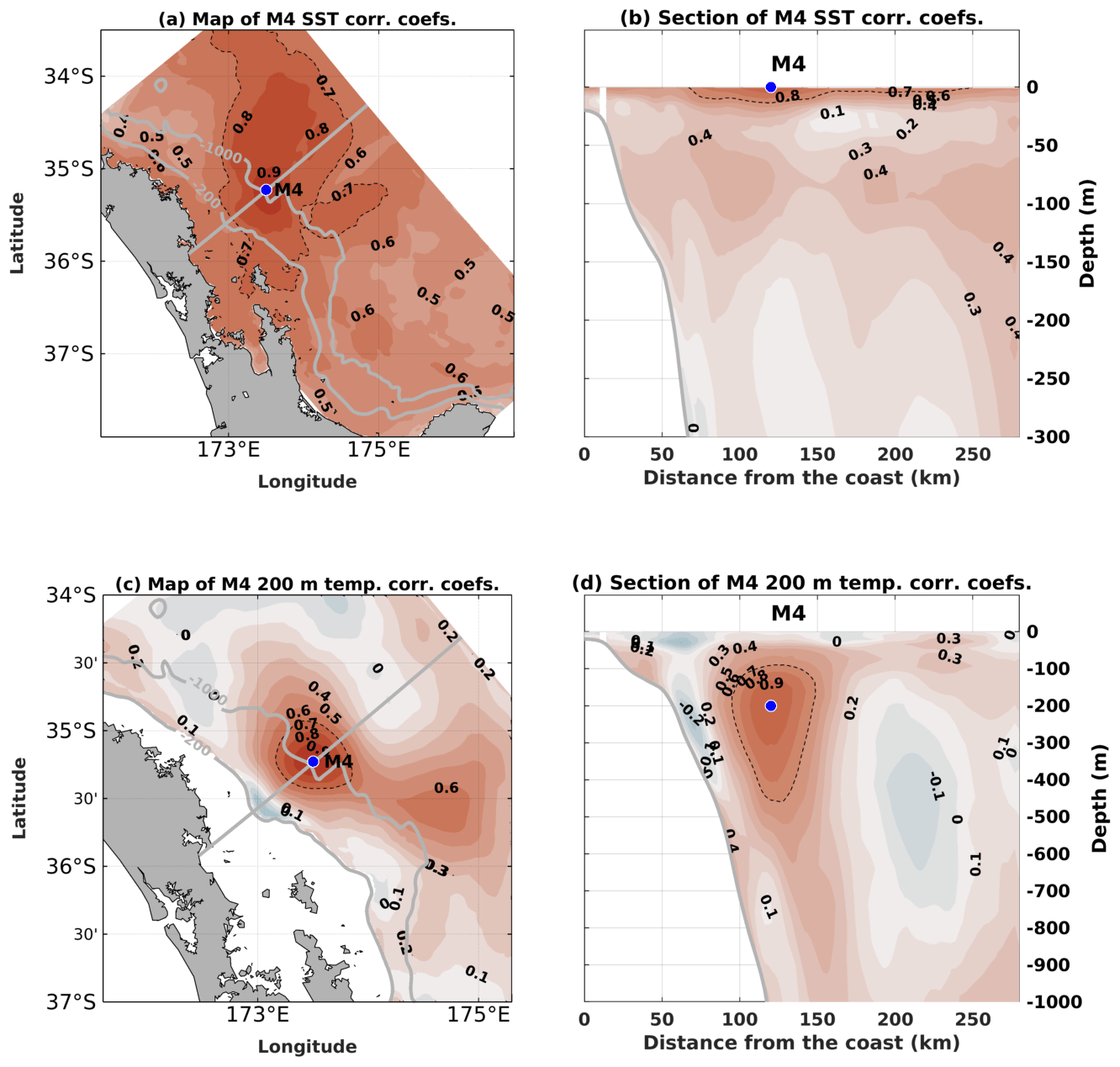
Figure 15Maps (a, c) and cross-sections (b, d) of linear correlation coefficients between surface (a, b) or 200 m (c, d) temperature at M4 and points in the rest of the domain from the NoDA run. The blue dots show observation locations used to correlate with surrounding model grid points. The dashed black line shows regions with correlation coefficients equal to 0.7. The cross-section used here follows the grid alignment, which is different from the moorings' orientation. The y axis in (b) and (d) is on the right-hand side for better visualisation.
Model temperature comparisons to Argo data showed similar results to comparisons at M4 and M5. NoTS and NoUVTS runs had a larger cold bias near 100 m depth, which generated a higher temperature RMSD (∼2 ∘C) in comparison to the NoDA run (∼1.6 ∘C). A warm bias was also evident around 600 m in all experiments with varying degrees. Assimilation of mooring temperature (ASFUVTS and NoUV) reduced the cold bias and the temperature RMSD (∼1 ∘C) in comparison to the NoDA run. The shallow cold and deeper warm biases are intrinsic to the NoDA run, which might be associated with biases in the boundary condition from HYCOM–NCODA when Argo data were not available (between June and September 2015) for assimilation north of 35∘ S. Even though larger temperature errors were observed in the simulations that withheld mooring temperature and salinity (1.6–2.1 ∘C), they were still comparable to freely evolving simulation temperature RMSD (∼1.9 ∘C) in other studies (e.g. Kerry et al., 2016; Siripatana et al., 2020) when assessed using Argo temperature.
Data assimilation of subsurface observations using a 7 d window and smaller decorrelation length scales had little impact in correcting salinity at the Argo locations. A small salinity degradation was simulated between 0 and 200 m in the assimilative experiments in comparison to the NoDA run. A negative impact on near-surface salinity was also observed when assimilating SST or SSH data only in the Brazil Current region (Santana et al., 2020). Some authors suggest that assimilation of salinity data is needed to constrain the model water column salinity (e.g. Oke and Schiller, 2007; Tanajura et al., 2014; Oke et al., 2015). Assimilation of surface and subsurface data every 2 d with a larger decorrelation length scale of tracers (ASFUVTS-2 d) was able to considerably correct model salinity below 400 m. The ASFUVTS-2 d run reached error values similar to HYCOM–NCODA, which assimilated salinity data from Argo floats.
Increments to temperature initial conditions were positive and deep (200 m) in the experiments that assimilated subsurface temperature (ASFUVTS and NoUV). In contrast, withholding in situ temperature (NoTS and NoUVTS) generated negative and shallower (50 m) increments. This generated differences in the atmospheric heat fluxes, where NoTS and NoUVTS had average positive heat flux in most of the domain to compensate for the negative increments to the temperature initial condition. The combined positive heat flux increments and negative temperature increments corrected the surface cold bias present in the NoDA run but not the cooling trend around 200 m. Conversely, experiments that assimilated subsurface temperature (ASFUVTS and NoUV) had negative average heat flux near the moorings. This negative heat flux balanced the positive temperature increment at M4 and M5, which aimed at correcting both surface and upper-thermocline (∼200 m) cold biases.
ASFUVTS, NoUV and ASFUVTS-2 d runs (assimilated subsurface temperature) had net-negative or near-zero surface heat flux varying from negative to positive flux from near to away from the moorings. This variability might be associated with the 4 d variances, which include the daily cycle of radiation and cloud coverage, and were used to compute the background error covariance of the forcing heat flux. Alternatively, there is a large spatial variability in heat flux that forced the NoDA run. It was positive north of 35∘ S and negative southwards. The NZNES is located near the zero heat flux line in the JRA55-do atmospheric forcing used in this study (Fig. 48 in Tsujino et al., 2018). For instance, the Hawaiian archipelago is also located near a zero-line heat flux in the atmospheric forcing product. 4D-Var experiments in the region also showed large average heat flux increments (±100 W m−2) and marked spatial variability with negative increments in the lee of the islands and positive increments to the west of them (Matthews et al., 2012).
Positive wind stress curl was generated on top of M5 when subsurface temperature data were assimilated (ASFUVTS and NoUV). Positive wind stress curl generates convergence and downwelling of warmer waters, which might be associated with corrections of the 200 m cold bias. Positive wind stress curl correction was also observed in the simulations on SE Brazil, which reduced the magnitude of upwelling in the region (de Paula et al., 2021). Changes in the wind stress curl in the ASFUVTS and NoUV runs (assimilated subsurface temperature) were also responsible for the lowered velocity complex correlation at M4 and M5 in comparison to the simulations that withheld subsurface temperature. If more subsurface salinity data were available, the solution ASFUVTS and NoUV runs could have converged to improved density structures that would have resulted in better-simulated currents, as we observed in ASFUVTS-2 d.
By running the OSEs we elucidate the importance of different datasets on the quality of ocean reanalyses. The representation of surface fields and consequent mesoscale eddies was improved by data assimilation of surface data only. The model high spatial resolution (2 km), which starts to resolve submesoscale processes, might be responsible for the lower skill compared to other 4D-Var regional studies that had lower horizontal resolution (>5 km). In our model, in situ subsurface temperature is of utmost importance to correctly simulate the top of the thermocline – one of the most difficult regions to simulate in ocean models. The lack of subsurface temperature for assimilation (NoTS and NoUVTS) increased the near-surface cold bias present in the freely evolving model run (NoDA). Assimilation of mooring temperature (ASFUVTS and NoUV) corrects this cold bias, even at distant Argo locations. Data assimilation using a 2 d window and doubled decorrelation length scales better matched the assimilated and independent observations. This approach must be used with care if subsurface data availability is low (e.g. using Argo floats only as subsurface data) because larger cold bias in the upper-thermocline can be generated (not shown). Nevertheless, all reanalyses showed improved velocity results on the mid-slope when compared to HYCOM–NCODA, which shows the importance of downscaling to better represent the slope bathymetry and possibly shelf–slope exchange.
The current work is part of a set of experiments that are preparing for a data assimilative ocean forecast for the NZNES. The computational cost to produce 1 d of reanalysis is about 52 min and 7 min to generate a 7 d forecast using 80 cores on the NeSI supercomputer (https://www.nesi.org.nz/, last access: 1 July 2023), a Cray XC50. Alongside the operational forecast development, improvements in the NoDA run configuration need to be conducted in order to understand and mitigate temperature and salinity biases. Tests should be conducted using the Mercator-Ocean forecast system (GLORYS) (Lellouche et al., 2018) as boundary conditions, since they showed better performance in comparison to HYCOM–NCODA (de Souza et al., 2021). New experiments based on the 7 d window configuration can be done using Argo and glider data. Questions regarding the absence or presence of glider data can be asked and the impact on the velocity field evaluated with observations. Continuous temperature and salinity sampling from ocean gliders would provide enough high vertical resolution and good spatial coverage to positively impact the simulation of the thermohaline field and ocean currents.
In the future, a posterior check of the consistency of the observation and background error hypotheses (Mattern et al., 2018) can be applied to improve the quality of the ocean reanalyses. Mattern et al. (2018) described how the covariance of residuals and innovations and the covariance of increments and innovations should be roughly equal to the assumed observation and background error variances, respectively. Posterior tests of these statistics probe whether the prior assumptions for error variances need adjusting to be consistent with the model intrinsic skill and representativeness error. This method has been applied to the GLORYS to obtain better performance (Lellouche et al., 2018). Moreover, an ensemble 4D-Var approach can be applied to improve the quality of the analysis on the NZNES. This methodology uses several perturbed simulations (ensemble) to estimate the model error covariance matrix (D) (e.g. Pasmans and Kurapov, 2019). This includes spatial and temporal variability to D compared to a fixed model covariance matrix used here. This method showed improved representation of glider temperature and salinity observations when compared to 4D-Var using a static D (Pasmans et al., 2020).
The Regional Ocean Modeling System (ROMS) is widely known in the modelling oceanographic community, and its source code, documentation and discussion forum can be found at https://www.myroms.org/ (Haidvogel et al., 2008). Configuration files and scripts for analysing model output can be found on https://doi.org/10.5281/zenodo.7306271 (Santana, 2022).
Moorings' dataset can be found in O'Callaghan et al. (2015) (https://doi.org/10.17882/78971). NIWA bathymetric data used in the model can be found on https://niwa.co.nz/oceans/resources/bathymetry/download-the-data (NIWA, 2016).
JO'C conducted the sampling experiment. HM set up the numerical model and lateral conditions. RS analysed the data, included new atmospheric forcing in the model, generated the data assimilative runs, analysed the results and wrote the paper. BP supervised the improvement of the reanalysis and provided SeaPy (Python library for ocean state estimate). RS, HM, JO'C, BP, SW and SHS discussed the results and reviewed the paper.
The contact author has declared that none of the authors has any competing interests.
Publisher’s note: Copernicus Publications remains neutral with regard to jurisdictional claims in published maps and institutional affiliations.
We thank everyone involved in data collection and curation at NIWA, as well as support from the New Zealand eScience Infrastructure (NeSI) that made this work possible. Funding was provided by the NIWA Strategic Science Investment Fund (SSIF) Ocean–Climate Interactions Programme, the Flows and Productivity Programme, and the MBIE endeavour Smart Ideas grant (CO1X1814). We also thank John Wilkin who provided extra comments that improved the manuscript.
This research has been supported by the NIWA Strategic Science Investment Fund (SSIF) Ocean-Climate Interactions Programme, the Flows and Productivity Programme, and the MBIE endeavour Smart Ideas grant (grant no. CO1X1814).
This paper was edited by Deepak Subramani and reviewed by Srinivasa Ramanujam Kannan and one anonymous referee.
Bannister, R.: A review of operational methods of variational and ensemble-variational data assimilation, Q. J. Roy. Meteor. Soc., 143, 607–633, 2017. a
Bowen, M. M., Wilkin, J. L., and Emery, W. J.: Variability and forcing of the East Australian Current, J. Geophys. Res.-Oceans, 110, C03019, https://doi.org/10.1029/2004JC002533, 2005. a
Casey, K. S., Brandon, T. B., Cornillon, P., and Evans, R.: The Past, Present, and Future of the AVHRR Pathfinder SST Program, Springer Netherlands, Dordrecht, 273–287, https://doi.org/10.1007/978-90-481-8681-5_16, 2010. a
Chapman, D. C.: Numerical treatment of cross-shelf open boundaries in a barotropic coastal ocean model, J. Phys. Oceanogr., 15, 1060–1075, 1985. a
Chassignet, E. P., Hurlburt, H. E., Metzger, E. J., Smedstad, O. M., Cummings, J. A., Halliwell, G. R., Bleck, R., Baraille, R., Wallcraft, A. J., Lozano, C., Tolman, H., Srinivasan, A., Hankin, S., Cornillon, P., Weisberg, R., Barth, A., He, R., Werner, F., and Wilkin, J.: US GODAE: global ocean prediction with the HYbrid Coordinate Ocean Model (HYCOM), Oceanography, 22, 64–75, 2009. a, b
Chiswell, S. M.: Determining the internal structure of the ocean off northeast New Zealand from surface measurements, New Zeal. J. Mar. Fresh., 35, 289–306, https://doi.org/10.1080/00288330.2001.9516999, 2001. a
Chiswell, S. M., Bostock, H. C., Sutton, P. J., and Williams, M. J.: Physical oceanography of the deep seas around New Zealand: a review, New Zeal. J. Mar. Fresh., 49, 286–317, https://doi.org/10.1080/00288330.2014.992918, 2015. a
de Paula, T. P., Lima, J. A. M., Tanajura, C. A. S., Andrioni, M., Martins, R. P., and Arruda, W. Z.: The impact of ocean data assimilation on the simulation of mesoscale eddies at Sao Paulo plateau (Brazil) using the regional ocean modeling system, Ocean Model., 167, 101889, https://doi.org/10.1016/j.ocemod.2021.101889, 2021. a, b, c, d, e
de Souza, J. M. A. C., Couto, P., Soutelino, R., and Roughan, M.: Evaluation of four global ocean reanalysis products for New Zealand waters–A guide for regional ocean modelling, New Zeal. J. Mar. Fresh., 55, 132–155, 2021. a, b
Di Lorenzo, E., Moore, A. M., Arango, H. G., Cornuelle, B. D., Miller, A. J., Powell, B., Chua, B. S., and Bennett, A. F.: Weak and strong constraint data assimilation in the inverse Regional Ocean Modeling System (ROMS): Development and application for a baroclinic coastal upwelling system, Ocean Model., 16, 160–187, 2007. a, b
Ducet, N., Le Traon, P. Y., and Reverdin, G.: Global high-resolution mapping of ocean circulation from TOPEX/Poseidon and ERS-1 and -2, J. Geophys. Res.-Oceans, 105, 19477–19498, https://doi.org/10.1029/2000JC900063, 2000. a
Fairall, C. W., Bradley, E. F., Hare, J., Grachev, A. A., and Edson, J. B.: Bulk parameterization of air–sea fluxes: Updates and verification for the COARE algorithm, J. Climate, 16, 571–591, 2003. a
Feng, M., Wijffels, S., Godfrey, S., and Meyers, G.: Do eddies play a role in the momentum balance of the Leeuwin Current?, J. Phys. Oceanogr., 35, 964–975, 2005. a
Fisher, M. and Courtier, P.: Estimating the covariance matrices of analysis and forecast error in variational data assimilation, ECMWF Tech. Mem. 220, https://doi.org/10.21957/1dxrasjit, 1995. a
Haidvogel, D. B., Arango, H., Budgell, W. P., Cornuelle, B. D., Curchitser, E., Di Lorenzo, E., Fennel, K., Geyer, W. R., Hermann, A. J., Lanerolle, L., Levin, J., McWilliams, J., Miller, A., Moore, A., Powell, T., Shchepetkin, A., Sherwood, R., Signell, W., Warner, J., and Wilkin, J.: Ocean forecasting in terrain-following coordinates: Formulation and skill assessment of the Regional Ocean Modeling System, J. Comput. Phys., 227, 3595–3624, 2008 (code available at: https://www.myroms.org/, last access: 4 July 2023). a, b
Kerry, C., Powell, B., Roughan, M., and Oke, P.: Development and evaluation of a high-resolution reanalysis of the East Australian Current region using the Regional Ocean Modelling System (ROMS 3.4) and Incremental Strong-Constraint 4-Dimensional Variational (IS4D-Var) data assimilation, Geosci. Model Dev., 9, 3779–3801, https://doi.org/10.5194/gmd-9-3779-2016, 2016. a, b, c, d, e, f, g, h, i
Kerry, C., Roughan, M., and Powell, B.: Predicting the submesoscale circulation inshore of the East Australian Current, J. Marine Syst., 204, 103286, 2020. a
Kundu, P. K.: Ekman Veering Observed near the Ocean Bottom, J. Phys. Oceanogr., 6, 238–242, https://doi.org/10.1175/1520-0485(1976)006<0238:EVONTO>2.0.CO;2, 1976. a
Laing, A. K., Oien, N. A., Murphy, R., and Uddstrom, M. J.: Coherent signals in the temperature and height of the sea surface off North Cape, New Zealand, New Zeal. J. Mar. Fresh., 32, 187–202, https://doi.org/10.1080/00288330.1998.9516819, 1998. a
Lellouche, J.-M., Greiner, E., Le Galloudec, O., Regnier, C., Benkiran, M., Testut, C.-E., Bourdalle-Badie, R., Drevillon, M., Garric, G., and Drillet, Y.: Mercator Ocean Global High-Resolution Monitoring and Forecasting System, New Frontiers in Operational Oceanography, 1, 563–592, 2018. a, b
Lentz, S. J.: Observations and a Model of the Mean Circulation over the Middle Atlantic Bight Continental Shelf, J. Phys. Oceanogr., 38, 1203–1221, https://doi.org/10.1175/2007JPO3768.1, 2008. a
Marchesiello, P., McWilliams, J. C., and Shchepetkin, A.: Open boundary conditions for long-term integration of regional oceanic models, Ocean Model., 3, 1–20, 2001. a
Marchesiello, P., McWilliams, J. C., and Shchepetkin, A.: Equilibrium structure and dynamics of the California Current System, J. Phys. Oceanogr., 33, 753–783, 2003. a
Mason, E., Molemaker, J., Shchepetkin, A. F., Colas, F., McWilliams, J. C., and Sangrà, P.: Procedures for offline grid nesting in regional ocean models, Ocean Model., 35, 1–15, https://doi.org/10.1016/j.ocemod.2010.05.007, 2010. a
Mata, M. M., Tomczak, M., Wijffels, S., and Church, J. A.: East Australian Current volume transports at 30∘ S: Estimates from the World Ocean Circulation Experiment hydrographic sections PR11/P6 and the PCM3 current meter array, J. Geophys. Res.-Oceans, 105, 28509–28526, https://doi.org/10.1029/1999JC000121, 2000. a
Mattern, J. P., Edwards, C. A., and Moore, A. M.: Improving variational data assimilation through background and observation error adjustments, Mon. Weather Rev., 146, 485–501, 2018. a, b
Matthews, D., Powell, B., and Janeković, I.: Analysis of four-dimensional variational state estimation of the Hawaiian waters, J. Geophys. Res.-Oceans, 117, C03013, https://doi.org/10.1029/2011JC007575, 2012. a
Mignac, D., Tanajura, C. A. S., Santana, A. N., Lima, L. N., and Xie, J.: Argo data assimilation into HYCOM with an EnOI method in the Atlantic Ocean, Ocean Sci., 11, 195–213, https://doi.org/10.5194/os-11-195-2015, 2015. a
Moore, A. M., Arango, H. G., Broquet, G., Powell, B. S., Weaver, A. T., and Zavala-Garay, J.: The Regional Ocean Modeling System (ROMS) 4-dimensional variational data assimilation systems: Part I–System overview and formulation, Prog. Oceanogr., 91, 34–49, 2011a. a, b, c, d, e, f, g, h
Moore, A. M., Arango, H. G., Powell, B., Broquet, G., Edwards, C., Veneziani, M., Foley, D., Doyle, J. D., Costa, D., and Robinson, P.: The Regional Ocean Modeling System (ROMS) 4-dimensional variational data assimilation systems: Part II–Performance and application to the California Current System, Prog. Oceanogr., 91, 50–73, 2011b. a, b
National Institute of Water and Atmospheric Research (NIWA): New Zealand's high resolution bathymetric data, https://niwa.co.nz/oceans/resources/bathymetry/download-the-data (last access: 5 July 2023), 2016. a
O'Callaghan, J., Mike, B., and Fiona, E.: Across-shelf mooring array from the northeast shelf of New Zealand, SEANOE [data set], https://doi.org/10.17882/78971, 2015. a, b
Oke, P., Schiller, A., Griffin, D., and Brassington, G.: Ensemble data assimilation for an eddy-resolving ocean model of the Australian region, Quarterly Journal of the Royal Meteorological Society: A journal of the atmospheric sciences, Appl. Meteorol. Phys. Oceanogr., 131, 3301–3311, 2005. a
Oke, P. R. and Schiller, A.: Impact of Argo, SST, and altimeter data on an eddy-resolving ocean reanalysis, Geophys. Res. Lett., 34, L19601, https://doi.org/10.1029/2007GL031549, 2007. a
Oke, P. R., Sakov, P., Cahill, M. L., Dunn, J. R., Fiedler, R., Griffin, D. A., Mansbridge, J. V., Ridgway, K. R., and Schiller, A.: Towards a dynamically balanced eddy-resolving ocean reanalysis: BRAN3, Ocean Model., 67, 52–70, 2013. a
Oke, P. R., Larnicol, G., Fujii, Y., Smith, G. C., Lea, D. J., Guinehut, S., Remy, E., Balmaseda, M. A., Rykova, T., Surcel-Colan, D., Martin, M., Sellar, A., Mulet, S., and Turpin, V.: Assessing the impact of observations on ocean forecasts and reanalyses: Part 1, Global studies, J. Oper. Oceanogr., 8, s49–s62, 2015. a, b, c
Oke, P. R., Roughan, M., Cetina-Heredia, P., Pilo, G. S., Ridgway, K. R., Rykova, T., Archer, M. R., Coleman, R. C., Kerry, C. G., Rocha, C., Schaeffer, A., and Vitarelli, E.: Revisiting the circulation of the East Australian Current: Its path, separation, and eddy field, Prog. Oceanogr., 176, 102139, https://doi.org/10.1016/j.pocean.2019.102139, 2019. a
Pasmans, I. and Kurapov, A. L.: Ensemble of 4DVARs (En4DVar) data assimilation in a coastal ocean circulation model, part I: methodology and ensemble statistics, Ocean Model., 144, 101493, 2019. a
Pasmans, I., Kurapov, A., Barth, J., Ignatov, A., Kosro, P., and Shearman, R.: Why Gliders Appreciate Good Company: Glider Assimilation in the Oregon-Washington Coastal Ocean 4DVAR System With and Without Surface Observations, J. Geophys. Res.-Oceans, 124, 750–772, 2019. a, b
Pasmans, I., Kurapov, A. L., Barth, J. A., Kosro, P. M., and Shearman, R. K.: Ensemble 4DVAR (En4DVar) data assimilation in a coastal ocean circulation model. Part II: Implementation offshore Oregon-Washington, USA, Ocean Model., 154, 101681, https://doi.org/10.1016/j.ocemod.2020.101681, 2020. a
Powell, B.: Quantifying how observations inform a numerical reanalysis of Hawaii, J. Geophys. Res.-Oceans, 122, 8427–8444, 2017. a
Powell, B., Arango, H., Moore, A., Di Lorenzo, E., Milliff, R., and Foley, D.: 4DVAR data assimilation in the intra-Americas sea with the Regional Ocean Modeling System (ROMS), Ocean Model., 23, 130–145, 2008. a
Rodi, W.: Examples of calculation methods for flow and mixing in stratified fluids, J. Geophys. Res.-Oceans, 92, 5305–5328, https://doi.org/10.1029/JC092iC05p05305, 1987. a
Roemmich, D. and Sutton, P.: The mean and variability of ocean circulation past northern New Zealand: Determining the representativeness of hydrographic climatologies, J. Geophys. Res.-Oceans, 103, 13041–13054, https://doi.org/10.1029/98JC00583, 1998. a
Roemmich, D., Alford, M. H., Claustre, H., Johnson, K., King, B., Moum, J., Oke, P., Owens, W. B., Pouliquen, S., Purkey, S., et al.: On the future of Argo: A global, full-depth, multi-disciplinary array, Front. Mar. Sci., 6, 439, https://doi.org/10.3389/fmars.2019.00439, 2019. a
Sandery, P. A. and Sakov, P.: Ocean forecasting of mesoscale features can deteriorate by increasing model resolution towards the submesoscale, Nat. Commun., 8, 1–8, 2017. a
Santana, R.: East Auckland Current ocean model configuration and analysis files, Zenodo [code], https://doi.org/10.5281/zenodo.7306271, 2022. a
Santana, R., Costa, F. B., Mignac, D., Santana, A. N., Vidal, V. F. d. S., Zhu, J., and Tanajura, C. A. S.: Model sensitivity experiments on data assimilation, downscaling and tides for the representation of the Cape São Tomé Eddies, Ocean Dynam., 70, 77–94, https://doi.org/10.1007/s10236-019-01307-w, 2020. a, b, c, d
Santana, R., Suanda, S., Macdonald, H., and O'Callaghan, J.: Mesoscale and wind-driven intra-annual variability in the East Auckland Current, Sci. Rep.-UK, 9764, https://doi.org/10.1038/s41598-021-89222-3, 2021. a, b, c, d, e, f, g, h, i, j, k, l, m, n, o, p, q
Shchepetkin, A. F. and McWilliams, J. C.: A method for computing horizontal pressure-gradient force in an oceanic model with a nonaligned vertical coordinate, J. Geophys. Res.-Oceans, 108, FET 4-1–FET 3-16, https://doi.org/10.1029/2001JC001047, 2003. a
Shchepetkin, A. F. and McWilliams, J. C.: The regional oceanic modeling system (ROMS): a split-explicit, free-surface, topography-following-coordinate oceanic model, Ocean Model., 9, 347–404, 2005. a, b
Shchepetkin, A. F. and McWilliams, J. C.: Computational kernel algorithms for fine-scale, multiprocess, longtime oceanic simulations, in: Handbook of Numerical Analysis, 14, 121–183, Elsevier, https://doi.org/10.1016/S1570-8659(08)01202-0, 2009. a
Siripatana, A., Kerry, C., Roughan, M., Souza, J. M. A. C., and Keating, S.: Assessing the Impact of Nontraditional Ocean Observations for Prediction of the East Australian Current, J. Geophys. Res.-Oceans, 125, e2020JC016580, https://doi.org/10.1029/2020JC016580, 2020. a, b, c
Sloyan, B. M., Ridgway, K. R., and Cowley, R.: The East Australian Current and Property Transport at 27∘ S from 2012 to 2013, J. Phys. Oceanogr., 46, 993–1008, https://doi.org/10.1175/JPO-D-15-0052.1, 2016. a
Stanton, B. and Sutton, P.: Velocity measurements in the East Auckland Current northeast of North Cape, New Zealand, New Zeal. J. Mar. Fresh., 37, 195–204, https://doi.org/10.1080/00288330.2003.9517157, 2003. a
Stanton, B. R. and Morris, M. Y.: Direct velocity measurements in the Subantarctic Front and over Campbell Plateau, southeast of New Zealand, J. Geophys. Res.-Oceans, 109, https://doi.org/10.1029/2002JC001339, 2004. a
Stanton, B. R., Sutton, P. J. H., and Chiswell, S. M.: The East Auckland Current, 1994-95, New Zeal. J. Mar. Fresh., 31, 537–549, https://doi.org/10.1080/00288330.1997.9516787, 1997. a
Taboada, F. G., Stock, C. A., Griffies, S. M., Dunne, J., John, J. G., Small, R. J., and Tsujino, H.: Surface winds from atmospheric reanalysis lead to contrasting oceanic forcing and coastal upwelling patterns, Ocean Model., 133, 79–111, https://doi.org/10.1016/j.ocemod.2018.11.003, 2019. a, b
Tanajura, C., Novaes Santana, A., Mignac, D., Nascimento Lima, L., Belyaev, K., and Ji-Ping, X.: The REMO ocean data assimilation system into HYCOM (RODAS_H): General description and preliminary results, Atmospheric and Oceanic Science Letters, 7, 464–470, 2014. a
Tsujino, H., Urakawa, S., Nakano, H., Small, R. J., Kim, W. M., Yeager, S. G., Danabasoglu, G., Suzuki, T., Bamber, J. L., Bentsen, M., et al.: JRA-55 based surface dataset for driving ocean–sea-ice models (JRA55-do), Ocean Model., 130, 79–139, 2018. a, b, c
Umlauf, L. and Burchard, H.: A generic length-scale equation for geophysical turbulence models, J. Marine Res., 61, 235–265, https://doi.org/10.1357/002224003322005087, 2003. a
Weaver, A. and Courtier, P.: Correlation modelling on the sphere using a generalized diffusion equation, Q. J. Roy. Meteor. Soc., 127, 1815–1846, 2001. a
Weaver, A., Vialard, J., and Anderson, D.: Three-and four-dimensional variational assimilation with a general circulation model of the tropical Pacific Ocean. Part I: Formulation, internal diagnostics, and consistency checks, Mon. Weather Rev., 131, 1360–1378, 2003. a
Xie, J. and Zhu, J.: Ensemble optimal interpolation schemes for assimilating Argo profiles into a hybrid coordinate ocean model, Ocean Model., 33, 283–298, 2010. a
Zavala-Garay, J., Wilkin, J., and Arango, H.: Predictability of mesoscale variability in the East Australian Current given strong-constraint data assimilation, J. Phys. Oceanogr., 42, 1402–1420, 2012. a, b, c, d
Zeldis, J. R., Walters, R. A., Greig, M. J., and Image, K.: Circulation over the northeastern New Zealand continental slope, shelf and adjacent Hauraki Gulf, during spring and summer, Cont. Shelf Res., 24, 543–561, https://doi.org/10.1016/j.csr.2003.11.007, 2004. a