AdaHRBF v1.0: gradient-adaptive Hermite–Birkhoff radial basis function interpolants for three-dimensional stratigraphic implicit modeling

Three-dimensional (3D) stratigraphic modeling is capable of modeling the shape, topology, and other properties of strata in a digitalized manner. The implicit modeling approach is becoming the mainstream approach for 3D stratigraphic modeling, which incorporates both the off-contact strike and dip directions and the on-contact occurrence information of stratigraphic interface to estimate the stratigraphic potential field (SPF) to represent the 3D architectures of strata. However, the magnitudes of the SPF gradient controlling the variation trend of SPF values cannot be directly derived from the known stratigraphic attribute or strike and dip data. In this paper, we propose a Hermite–Birkhoff radial basis function (HRBF) formulation, AdaHRBF, with an adaptive gradient magnitude for continuous 3D SPF modeling of multiple stratigraphic interfaces. In the linear system of HRBF interpolants constrained by the scattered on-contact attribute points and off-contact strike and dip points of a set of strata in 3D space, we add a novel optimizing term to iteratively obtain the optimized gradient magnitude. The case study shows that the HRBF interpolants can consistently and accurately establish multiple stratigraphic interfaces and fully express the internal stratigraphic attribute and orientation. To ensure harmony of the variation in stratigraphic thickness, we adopt the relative burial depth of the stratigraphic interface to the Quaternary as the SPF attribute value. In addition, the proposed stratigraphic-potential-field modeling by HRBF interpolants can provide a suitable basic model for subsequent geosciences' numerical simulation.

1 Introduction

The three-dimensional (3D) stratigraphic modeling and visualization technology is of great importance for the intelligent management of subsurface space (e.g., mineral resource assessment, reservoir characterization, groundwater management, and urban subsurface space planning) (Houlding, 1994; Mallet, 2002). The two main ways of representing 3D stratigraphic surface are so-called explicit and implicit modeling (Lajaunie et al., 1997). Traditional explicit modeling can be described as a way of representing 3D geological boundaries that relies heavily on a complicated and time-consuming process of human–computer interaction for connecting the geological boundary lines to form a 3D model of geological surfaces, and it is difficult to update the model. Implicit modeling defines a continuous 3D stratigraphic potential field (SPF) that describes the stratigraphic distribution and represents geological boundaries using an implicit mathematical function. The increasing importance of an implicit method in stratigraphic modeling stems from not only the advantages of efficiency, reproducibility, and topological consistency over the traditional explicit modeling method but also the full representation of stratigraphic structure through SPF. Although implicit modeling often requires a large solution system of linear equations to consume more computational time than explicit modeling, e.g., the Delaunay triangulation (Mallet, 2002; De Berg et al., 2008), we can overcome this difficulty with the help of increasing computational ability of computers. Three-dimensional stratigraphic-potential-field modeling is to implicitly represent the nature, shape, topology, and internal property of a given set of strata. The stratigraphic interface is expressed by a specific equipotential surface of the SPF. Therefore, using SPF to express a set of conformable strata and their attribute distribution in 3D space is convenient for spatial analysis, statistics, and simulation.

The strike and dip information can be incorporated into implicit modeling by setting up the gradients of implicit function. To control the orientation of the modeled strata, the dip and strike directions are encoded as the gradient directions. The difference between Hermite–Birkhoff radial basis function (HRBF) and standard radial basis function (RBF) is the presence of gradients; however, the existing HRBF method constructs implicit field functions separately for each geological interface and extracts the zero-value equipotential surfaces to locate the geological interface. Therefore, it is difficult to maintain topological and semantic consistency between geological bodies. For modeling multiple strata in an integrated and unique framework, however, setting up the gradient magnitudes to be adaptive to the orientation and thickness variations in strata is rather challenging. Assigning the adaptive gradient magnitudes to HRBF interpolant function is a “chicken-and-egg” problem: while the implicit function results from the gradients, the suitable gradient magnitudes are estimated from the reasonable implicit function.

In this study, we propose a gradient-adaptive HRBF framework for SPF modeling, AdaHRBF, which interpolates multiple interfaces among a set of conformable strata by a unified one-step process. In this linear system of HRBF interpolants, we iteratively obtain the optimized gradient magnitudes. The particular case where the SPF was reconstructed from geological maps and cross-sections demonstrates the advantages and general performance of stratigraphic-potential-field modeling using the AdaHRBF method, comparing with HRBF interpolants using constant unit normal gradients and RBF interpolants only using contact locations without orientations. The SPF attribute value is set to the relative burial depth of strata, i.e., mean distance from a given stratigraphic surface to the top surface of the Quaternary. The distributions of burial depth, thickness, and strike and dip of strata in 3D space can be fully expressed by the SPF and its gradient vector field.

2 Related works

The key of implicit modeling methods is to interpolate a 3D scalar field function whose equipotential surfaces indicate the boundaries of geological bodies. These surfaces can represent ore-grade boundaries or stratigraphic interfaces. This scalar field is interpolated from stratigraphic interface points and strike and dip data with either discrete-interpolation schemes or continuous-interpolation schemes.

2.1 Discrete interpolants

For discrete-interpolation schemes of implicit modeling with a special mesh, the GoCAD (https://app.pdgm.com/product-category/skua-gocad/, last access: 30 June 2022) software was developed based on the discrete smooth interpolation (DSI) method to meet the needs of geological, geophysical, and petroleum reservoir engineering modeling (Mallet, 2004; Frank et al., 2007). Caumon et al. (2013) proposed a discretizing finite-element method (FEM) to generate 3D models of horizons on a tetrahedral mesh, using stratigraphic interface traces of unknown attribute values and strike and dip measurements from 2D geological maps, remote sensing images, and digital elevation models. Hillier et al. (2013) presented a structural field interpolation (SFI) algorithm using an anisotropic inverse distance-weighted (IDW) interpolation scheme derived from eigen analysis of strike and dip measurements. Renaudeau et al. (2019) proposed an implicit structural modeling method using locally defined moving-least-squares shape functions and solved a sparse sampling problem without relying on a complex mesh. Irakarama et al. (2020) introduced a new method for implicit structural modeling by regularization operators on the Cartesian grid using finite differences. Grose et al. (2021b) presented LoopStructural, a new open-source 3D geological modeling Python package, in which discrete interpolators and polynomial trend interpolators can be mixed and matched within a geological model.

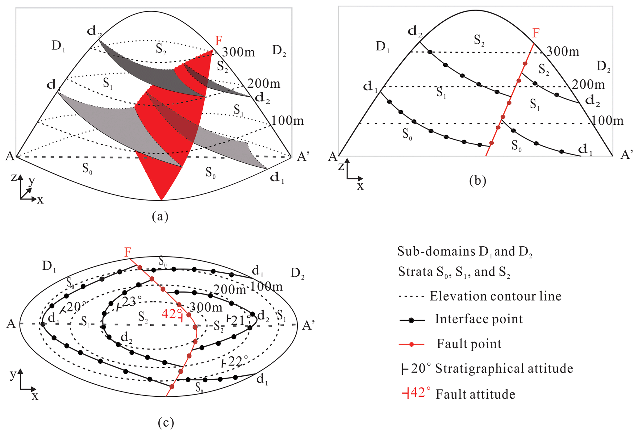
Figure 1 Data commonly used in (a) 3D geological modeling extracted from (b) cross-sections and (c) geological maps. A stratum S1 is between its bottom surface d₁ and top surface d₂ (Fig. 1a); a fault interface F divides the 3D space into two sub-domains, D₁ and D₂. We can extract the on-contact boundary points and off-contact strike and dip points of the strata and fault from the cross-section AA^′ (b) and geological map (c).

2.2 Continuous interpolants

Since the continuous-interpolation scheme does not depend on a mesh for its definition, the stratigraphic interfaces can be extracted at any desired resolution in the specific volume of interest. There is already a dual kriging or cokriging formulation for continuous potential-field modeling of multiple stratigraphic interfaces. Lajaunie et al. (1997) proposed an implicit potential-field modeling method using the dual formulation of kriging interpolation that considers known points on a geological interface and plane strike and dip data such as stratification or foliation planes. Calcagno et al. (2008) cokriged the location of geological interfaces and strike and dip data from a structural field to interpolate a continuous 3D potential-field scalar function describing the geometry of geological bodies. Geomodeller 3D (http://www.geomodeller.com, last access: 30 June 2022), an implicit geological modeling application, utilizes the implicit potential-field method by cokriging or the dual formulation of kriging (Lindsay et al., 2012; Hassen et al., 2016). Gonçalves et al. (2017) proposed a vector potential-field solution from a machine learning perspective, recasting the problem as multivariate classification in a compositional data framework, which alleviates some of the assumptions of the cokriging method. De la Varga et al. (2019) presented GemPy (https://github.com/cgre-aachen/gempy, last access: 30 June 2022), an open-source implementation, to generate 3D geological models based on an implicit potential-field cokriging interpolation approach and to enable stochastic geological modeling and inversions of gravity and topology in machine learning and Bayesian inference frameworks. To reduce the impact of regularly occurring modeling artifacts that result from data configuration and uncertainty, Von Harten et al. (2021) proposed an approach that is a combination of an implicit interpolation algorithm with a local smoothing method based on the concepts of nugget effect and filtered kriging known from conventional geostatistics.

For continuous radial basis function (RBF) or HRBF interpolation schemes of implicit modeling without a mesh, Cowan et al. (2003) constructed an implicit model of the orebody or stratigraphic interface using a volumetric RBF interpolation function with an equipotential surface that includes the interface points and conventionally assigned an attribute value of zero and a “±” sign to indicate the inside and outside of the interface. Hillier et al. (2014, 2016) presented a generalized interpolation framework using RBF in Surfe, an open-source library, to implicitly model 3D continuous geological interfaces from on-surface points with gradient constraints as defined by strike–dip data with assigned polarity. Leapfrog Geo (http://www.leapfrog3d.com, last access: 30 June 2022) is an implicit geological modeling software package that models scattered data for interfaces using fast RBF interpolation methods (Vollgger et al., 2015; Basson et al., 2016, 2017; Creus et al., 2018; Stoch et al., 2020). Martin and Boisvert (2017) developed a RBF-based implicit modeling framework using domain decomposition to locally vary orientations and magnitudes of anisotropy for geological boundary models. Zhong et al. (2019, 2021) introduced combination constraints for modeling ore bodies based on multiple implicit field interpolation through RBF methods, in which a multiply labeled implicit function was defined that combines different implicit sub-fields by the combination operations to construct constraints honoring geological relationships more flexibly. Guo et al. (2016, 2018, 2020, 2021) proposed an explicitly and implicitly integrated 3D geological modeling approach for the geometric fusion of different types of complex geological structure models; therein, the HRBF-based implicit method was used to model general strata, faults, and folds, and the skinning method and the free-form surface were used to model local detailed structures. Wang et al. (2018) proposed an implicit modeling approach to automatically build a 3D model for orebodies by means of spatial HRBF interpolation directly based on geological borehole data.

However, the above RBF and HRBF interpolants, which use only the on-contact point datasets for each geological interface or assign an approximate gradient vector for each on-contact point according to its nearest strike and dip measurements, cannot be accurately consistent with actual strike and dip survey data. To maintain topological consistency between geological bodies and represent their internal burial depth and structural orientations, our AdaHRBF interpolation scheme yields an HRBF linear system that is analogous in form to the previously developed implicit potential-field interpolation method based on cokriging of contact increments using parametric isotropic covariance functions.

3 Methodology

3.1 Modeling constraints

The geological boundaries and structural orientations on planar geological maps and cross-sections are the most common data used for 3D geological modeling. Besides the geological boundaries extracted from boreholes, cross-sections, and geological maps, structural orientation (including strike direction, dip direction, and dip angle) data from geological maps play important roles in characterizing the shape and distribution of geological bodies, as shown in Fig. 1. The SPF modeling method can jointly reconstruct a 3D geological model using these data extracted from geological maps and cross-sections.

A field in a spatial domain Rⁿ defines the function f=f(p) at a point p∈Rⁿ in domain Rⁿ, and f(p) is also called field function. The SPF defines the 3D space as a scalar function f(p) at any point p; meanwhile, the stratigraphic interfaces are simulated and expressed as specific equipotential surfaces satisfying $f\left(p\right)=f_k(i=\mathrm{1},$ …, K) in the SPF. In practice, this specific function value f_k may correspond to the age of the stratigraphic interface or a relative distance from a reference interface (Mallet, 2004). Therefore, a stratum occupies the space between its bottom surface f_k and top surface f_k+1, while there are countless disjoint equipotential surfaces in each stratum (Mallet, 2004). A well-known problem is how to interpolate unknown points by a function f(⋅) using known points of the space Rⁿ. The key problem of SPF modeling is to obtain surfaces that are consistent with known on-contact points on the stratigraphic interfaces and the off-contact strike and dip directions of the strata. The stratigraphic interface points define the distribution of reference equipotential surfaces, while the strike and dip points define the gradient vectors of the scalar field.

The SPF modeling by the HRBF interpolant satisfies both the on-contact attribute constraint and off-contact strike and dip constraint. To fit an implicitly defined SPF from known attribute values ${\left\{\left({\mathit{p}}_i,f_i\right)\right\}}_{i=\mathrm{1}}^N\in {\mathbf{R}}^n\times R$ and gradients $({\mathit{p}}_j,{\mathbf{g}}_j){\mathit{\}}}_{j=\mathrm{1}}^M\in {\mathbf{R}}^n\times {\mathbf{R}}^n$ derived from strike and dip data, we can search for a function $f:{\mathbf{R}}^n\to R$ which satisfies both the on-contact constraints f(p_i)=f_i for each $i=\mathrm{1},\mathrm{\dots },N$ and the off-contact gradient constraints ∇f(p_j)=g_j for each j=1, …, M. In particular, ${\mathit{p}}_i=\left[\begin{array}{lll}{p}_i^x& p_i^y& p_i^z\end{array}\right]$, and ${\mathbf{g}}_j=\left[\begin{array}{lll}{g}_j^x& g_j^y& g_j^z\end{array}\right]$ in space R³.

3.2 HRBF interpolant

Generally, the basic RBF reconstructs an implicit function with constraint f(p_i)=f_i; however, the HRBF reconstructs an implicit function which interpolates scattered multivariate Hermite–Birkhoff data (i.e., unstructured points and orientations) (Macedo et al., 2011). With the joint constraints of f(p_i)=f_i and ∇f(p_j)=g_j, the optional solution is to obtain equipotential surfaces that are as smooth as possible, that is, to ensure the energy function, which represents the degree of equipotential surface smoothness and unevenness of SPF, is as small as possible. Therefore, the energy function E of the SPF is defined by further combining the thin-plate regularizer of f (Wahba, 1990; Walder et al., 2006) as

$$\begin{array}{}\text{(1)}& \begin{array}{rl}E& =\sum _{i=\mathrm{1}}^N{\left(f\left({\mathit{p}}_i\right)-f_i\right)}^{\mathrm{2}}+\sum _{j=\mathrm{1}}^M{\left({\displaystyle \frac{\partial f\left({\mathit{p}}_j\right)}{\partial x}}-g_j^x\right)}^{\mathrm{2}}\\ & +{\left({\displaystyle \frac{\partial f\left({\mathit{p}}_j\right)}{\partial y}}-g_j^y\right)}^{\mathrm{2}}+{\left({\displaystyle \frac{\partial f\left({\mathit{p}}_j\right)}{\partial z}}-g_j^z\right)}^{\mathrm{2}}\\ & +\underset{R}{\overset{\mathrm{3}}{\int }}{\displaystyle \frac{{\partial }^{\mathrm{2}}f\left(\mathit{p}\right)}{{\partial }^{\mathrm{2}}x}}+{\displaystyle \frac{{\partial }^{\mathrm{2}}f\left(\mathit{p}\right)}{{\partial }^{\mathrm{2}}y}}+{\displaystyle \frac{{\partial }^{\mathrm{2}}f\left(\mathit{p}\right)}{{\partial }^{\mathrm{2}}z}}\\ & +\mathrm{2}{\displaystyle \frac{{\partial }^{\mathrm{2}}f\left(\mathit{p}\right)}{\partial x\partial y}}+\mathrm{2}{\displaystyle \frac{{\partial }^{\mathrm{2}}f\left(\mathit{p}\right)}{\partial y\partial z}}+\mathrm{2}{\displaystyle \frac{{\partial }^{\mathrm{2}}f\left(\mathit{p}\right)}{\partial z\partial x}}\mathrm{d}x\mathrm{d}y\mathrm{d}z,\end{array}\end{array}$$

where $\frac{\partial f\left({\mathit{p}}_j\right)}{\partial x}$, $\frac{\partial f\left({\mathit{p}}_j\right)}{\partial y}$, and $\frac{\partial f\left({\mathit{p}}_j\right)}{\partial z}$ are the first-order partial derivatives of implicit function f(p) at point p_j, and $\frac{{\partial }^{\mathrm{2}}f\left(\mathit{p}\right)}{{\partial }^{\mathrm{2}}x}$, $\frac{{\partial }^{\mathrm{2}}f\left(\mathit{p}\right)}{{\partial }^{\mathrm{2}}y}$, $\frac{{\partial }^{\mathrm{2}}f\left(\mathit{p}\right)}{{\partial }^{\mathrm{2}}z}$, $\frac{{\partial }^{\mathrm{2}}f\left(\mathit{p}\right)}{\partial x\partial y}$, $\frac{{\partial }^{\mathrm{2}}f\left(\mathit{p}\right)}{\partial y\partial z}$, and $\frac{{\partial }^{\mathrm{2}}f\left(\mathit{p}\right)}{\partial z\partial x}$ are the second-order partial derivatives of implicit function f(p). The first and second components of energy function represent the misfit between the estimated values and observed contact and orientation points, respectively, and the third component of a second-order derivative of implicit function guarantees the smoothness of SPF implicit function.

When using the HRBF interpolation method, we usually add a first-order polynomial C(p) to ensure the smoothness and continuity of equipotential surfaces. In particular, $C\left(\mathit{p}\right)=c_{\mathrm{1}}+c_{\mathrm{2}}{\mathit{p}}^x+c_{\mathrm{3}}{\mathit{p}}^y+c_{\mathrm{4}}{\mathit{p}}^z$. The HRBF interpolation function has a concrete estimation form f^∗(p):

$$\begin{array}{}\text{(2)}& {\displaystyle }\begin{array}{rl}{f}^{\ast }\left(\mathit{p}\right)& =\sum _{i=\mathrm{1}}^N{\mathit{\alpha }}_i\mathit{\phi }\left(∥\mathit{p}-{\mathit{p}}_i∥\right)\\ & +\sum _{j=\mathrm{1}}^M\langle {\mathit{\beta }}_j,{\mathrm{\nabla }}_{\mathit{\phi }}\left(∥\mathit{p}-\mathit{p}∥\right)\rangle +C\left(\mathit{p}\right)\end{array}\text{(3)}& {\displaystyle }\begin{array}{rl}\mathrm{\nabla }{f}^{\ast }\left(\mathit{p}\right)& =\sum _{i=\mathrm{1}}^N{\mathit{\alpha }}_i\mathrm{\nabla }\mathit{\phi }\left(∥\mathit{p}-{\mathit{p}}_i∥\right)\\ & +\sum _{j=\mathrm{1}}^M{\mathrm{\nabla }}^{\mathrm{2}}\mathit{\phi }\left(∥\mathit{p}-{\mathit{p}}_j∥\right){\mathit{\beta }}_j+\mathrm{\nabla }C\left(\mathit{p}\right)\end{array},\end{array}$$

where ∥p−p_i∥ denotes the Euclidean distance between locations p and p_i; φ(r) is the radial basis function, herein, for which the cubic function φ(r)=r³ is used in this study; ∇ is the Hamiltonian operator; ∇² is the Hessian operator, in particular, $\mathbf{\nabla }={\left[\begin{array}{lll}\frac{\partial }{\partial x}& \frac{\partial }{\partial y}& \frac{\partial }{\partial z}\end{array}\right]}^T$ and ${\mathbf{\nabla }}^{\mathrm{2}}=\left[\begin{array}{lll}\frac{{\partial }^{\mathrm{2}}}{{\partial }^{\mathrm{2}}x}& \frac{{\partial }^{\mathrm{2}}}{\partial x\partial y}& \frac{{\partial }^{\mathrm{2}}}{\partial x\partial z}\\ \frac{{\partial }^{\mathrm{2}}}{\partial y\partial x}& \frac{{\partial }^{\mathrm{2}}}{{\partial }^{\mathrm{2}}y}& \frac{{\partial }^{\mathrm{2}}}{\partial y\partial z}\\ \frac{{\partial }^{\mathrm{2}}}{\partial z\partial x}& \frac{{\partial }^{\mathrm{2}}}{\partial z\partial y}& \frac{{\partial }^{\mathrm{2}}}{{\partial }^{\mathrm{2}}z}\end{array}\right]$; and 〈a,b〉 is the inner product of vectors a and b. The scalar weight coefficients α_i∈R, vector weight coefficients β_j∈Rⁿ, and $\mathbf{c}\in {\mathbf{R}}^{n+\mathrm{1}}$ (in particular, ${\mathit{\beta }}_j={\left[\begin{array}{lll}{\mathit{\beta }}_j^x& {\mathit{\beta }}_j^y& {\mathit{\beta }}_j^z\end{array}\right]}^T$ and $\mathbf{c}={\left[\begin{array}{llll}{c}_{\mathrm{1}}& c_{\mathrm{2}}& c_{\mathrm{3}}& c_{\mathrm{4}}\end{array}\right]}^T)$ are unknown and uniquely determined by the joint constraints $f^{\ast }\left({\mathit{p}}_i\right)=f_i$ for each i=1, …, N and $\mathrm{\nabla }{f}^{\ast }\left({\mathit{p}}_j\right)={\mathbf{g}}_j$ for each j=1, …, M.

The HRBF interpolant defines the implicit function as a sum of chosen basic functions with their linear weights. Furthermore, the type of basic functions (e.g., Gaussian, multi-quadric, and thin-plate spline) affects the result of spatial interpolation (Wendland, 2005; Rasmussen and Williams, 2006), which is split into two categories, i.e., strictly positive definite (SPD) and conditionally positive definite (CPD) functions (Hillier et al., 2014). We adopt the cubic function as the basis function in this study, i.e., φ(R)=r³, since it minimizes the curvature in three dimensions (Eq. 1).

According to the joint constraints, the weight coefficients α, β, and c of the interpolant are determined by the following linear system:

$$\begin{array}{}\text{(4)}& \left[\begin{array}{lll}\mathbf{\Phi }& \mathrm{\nabla }\mathbf{\Phi }& \mathbf{C}\\ (\mathrm{\nabla }\mathbf{\Phi }{)}^{\mathrm{T}}& {\mathbf{\nabla }}^{\mathrm{2}}\mathbf{\Phi }& \mathrm{\nabla }\mathbf{C}\\ {\mathbf{C}}^{\mathrm{T}}& (\mathrm{\nabla }\mathbf{C}{)}^{\mathrm{T}}& \mathbf{0}\end{array}\right]\left[\begin{array}{l}\mathit{\alpha }\\ \mathit{\beta }\\ \mathbf{c}\end{array}\right]=\left[\begin{array}{l}\mathbf{f}\\ \mathbf{g}\\ \mathbf{0}\end{array}\right],\end{array}$$

where

$$\mathbf{\Phi }={\left[\begin{array}{cccc}{\mathit{\phi }}_{\mathrm{11}}& {\mathit{\phi }}_{\mathrm{12}}& \mathrm{\cdots }& {\mathit{\phi }}_{\mathrm{1}N}\\ {\mathit{\phi }}_{\mathrm{21}}& {\mathit{\phi }}_{\mathrm{22}}& \mathrm{\cdots }& {\mathit{\phi }}_{\mathrm{2}N}\\ \mathrm{⋮}& \mathrm{⋮}& \mathrm{\ddots }& \mathrm{⋮}\\ {\mathit{\phi }}_{N\mathrm{1}}& {\mathit{\phi }}_{N\mathrm{2}}& \mathrm{\cdots }& {\mathit{\phi }}_{NN}\end{array}\right]}_{N\times N},$$

whose element ${\mathit{\phi }}_{ij}=\mathit{\phi }\left(∥{\mathit{p}}_i-{\mathit{p}}_j∥\right)$ represents the RBF value between a pair of contact points;

$$\mathrm{\nabla }\mathbf{\Phi }={\left[\begin{array}{cccc}\mathrm{\nabla }{\mathit{\phi }}_{\mathrm{11}}& \mathrm{\nabla }{\mathit{\phi }}_{\mathrm{12}}& \mathrm{\cdots }& \mathrm{\nabla }{\mathit{\phi }}_{\mathrm{1}M}\\ \mathrm{\nabla }{\mathit{\phi }}_{\mathrm{21}}& \mathrm{\nabla }{\mathit{\phi }}_{\mathrm{22}}& \mathrm{\cdots }& \mathrm{\nabla }{\mathit{\phi }}_{\mathrm{2}M}\\ \mathrm{⋮}& \mathrm{⋮}& \mathrm{\ddots }& \mathrm{⋮}\\ \mathrm{\nabla }{\mathit{\phi }}_{N\mathrm{1}}& \mathrm{\nabla }{\mathit{\phi }}_{N\mathrm{2}}& \mathrm{\cdots }& \mathrm{\nabla }{\mathit{\phi }}_{NM}\end{array}\right]}_{N\times nM},$$

whose element $\mathrm{\nabla }{\mathit{\phi }}_{ij}=\mathrm{\nabla }\mathit{\phi }\left(∥{\mathit{p}}_i-{\mathit{p}}_j∥\right)$ represents the differential RBF value between a contact point and an orientation point;

$${\mathbf{\nabla }}^{\mathrm{2}}\mathbf{\Phi }={\left[\begin{array}{cccc}{\mathrm{\nabla }}^{\mathrm{2}}{\mathit{\phi }}_{\mathrm{11}}& {\mathrm{\nabla }}^{\mathrm{2}}{\mathit{\phi }}_{\mathrm{12}}& \mathrm{\cdots }& {\mathrm{\nabla }}^{\mathrm{2}}{\mathit{\phi }}_{\mathrm{1}M}\\ {\mathrm{\nabla }}^{\mathrm{2}}{\mathit{\phi }}_{\mathrm{21}}& {\mathrm{\nabla }}^{\mathrm{2}}{\mathit{\phi }}_{\mathrm{22}}& \mathrm{\cdots }& {\mathrm{\nabla }}^{\mathrm{2}}{\mathit{\phi }}_{\mathrm{2}M}\\ \mathrm{⋮}& \mathrm{⋮}& \mathrm{\ddots }& \mathrm{⋮}\\ {\mathrm{\nabla }}^{\mathrm{2}}{\mathit{\phi }}_{M\mathrm{1}}& {\mathrm{\nabla }}^{\mathrm{2}}{\mathit{\phi }}_{M\mathrm{2}}& \mathrm{\cdots }& {\mathrm{\nabla }}^{\mathrm{2}}{\mathit{\phi }}_{MM}\end{array}\right]}_{nM\times nM},$$

whose element ${\mathrm{\nabla }}^{\mathrm{2}}{\mathit{\phi }}_{ij}={\mathrm{\nabla }}^{\mathrm{2}}\mathit{\phi }\left(∥{\mathit{p}}_i-{\mathit{p}}_j∥\right)$ represents the second-order differential RBF value between a pair of orientation points, C=C(p), in particular,

$$\begin{array}{c}{\displaystyle }\mathbf{C}={\left[\begin{array}{cccc}\mathrm{1}& p_{\mathrm{1}}^x& p_{\mathrm{1}}^y& p_{\mathrm{1}}^z\\ \mathrm{1}& p_{\mathrm{2}}^x& p_{\mathrm{2}}^y& p_{\mathrm{2}}^z\\ \mathrm{⋮}& \mathrm{⋮}& \mathrm{⋮}& \mathrm{⋮}\\ \mathrm{1}& p_N^x& p_N^y& p_N^z\end{array}\right]}_{N\times (n+\mathrm{1})}\\ {\displaystyle }\text{and}\\ {\displaystyle }\mathbf{\nabla }\mathit{C}={\left[\begin{array}{cccc}\mathbf{0}& \mathrm{\nabla }{p}_{\mathrm{1}}^x& \mathrm{\nabla }{p}_{\mathrm{1}}^y& \mathrm{\nabla }{p}_{\mathrm{1}}^z\\ \mathbf{0}& \mathrm{\nabla }{p}_{\mathrm{2}}^x& \mathrm{\nabla }{p}_{\mathrm{2}}^y& \mathrm{\nabla }{p}_{\mathrm{2}}^z\\ \mathrm{⋮}& \mathrm{⋮}& \mathrm{⋮}& \mathrm{⋮}\\ \mathbf{0}& \mathrm{\nabla }{p}_M^x& \mathrm{\nabla }{p}_M^y& \mathrm{\nabla }{p}_M^z\end{array}\right]}_{nM\times (n+\mathrm{1})},\end{array}$$

whose elements are $\mathrm{\nabla }{p}_i^x={\left[\begin{array}{lll}\mathrm{1}& \mathrm{0}& \mathrm{0}\end{array}\right]}^T$, $\mathrm{\nabla }{p}_i^y={\left[\begin{array}{lll}\mathrm{0}& \mathrm{1}& \mathrm{0}\end{array}\right]}^T$, and $\mathrm{\nabla }{p}_i^z={\left[\begin{array}{lll}\mathrm{0}& \mathrm{0}& \mathrm{1}\end{array}\right]}^T$, respectively.

$$\begin{array}{c}{\displaystyle }\mathit{\alpha }={\left[\begin{array}{cccc}{\mathit{\alpha }}_{\mathrm{1}}& {\mathit{\alpha }}_{\mathrm{2}}& \mathrm{\cdots }& {\mathit{\alpha }}_N\end{array}\right]}^T;\mathit{\beta }={\left[\begin{array}{cccc}{\mathit{\beta }}_{\mathrm{1}}& {\mathit{\beta }}_{\mathrm{2}}& \mathrm{\cdots }& {\mathit{\beta }}_M\end{array}\right]}^{\mathrm{T}};\\ {\displaystyle }\mathbf{f}={\left[\begin{array}{llll}{f}_{\mathrm{1}}& f_{\mathrm{2}}& \mathrm{\cdots }& f_N\end{array}\right]}^T;\text{ and }\mathbf{g}={\left[\begin{array}{llll}{\mathbf{g}}_{\mathrm{1}}& {\mathbf{g}}_{\mathrm{2}}& \mathrm{\dots }& {\mathbf{g}}_M\end{array}\right]}^T.\end{array}$$

Once we have the weight coefficients (α_i, β_j) and the polynomial coefficients (c₁, c₂, c₃, c₄) by solving the above HRBF linear system, we can substitute the weight coefficients and polynomial coefficients into the HRBF equations; then the interpolant function f(p) and its gradient function ∇f(p) can be easily obtained.

3.3 Adaptive gradient constraint

3.3.1 Determination of gradient direction

The gradient of the SPF is an important feature of stratum shape because it indicates the strike and dip of a stratum. For construction of a scalar field f(p), the gradient constraints ∇f(p_j)=g_j can also be added into modeling process (Caumon et al., 2013; Hillier et al., 2014). As shown in Fig. 2, the gradient vector g of SPF and the normal vector n of the stratigraphic interface have the same direction, which can be obtained through geological observation.

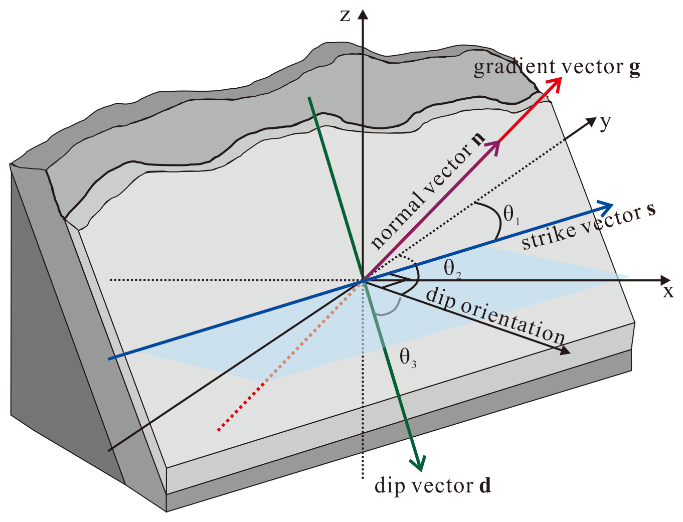
Figure 2 The gradient vector g, the strike vector s, and the dip vector d. The gradient vector g, the strike vector s, and the dip vector d of the SPF are orthogonal to each other. The strike θ₁ is the direction of the intersection of the stratigraphic interface and horizontal plane, which is represented by the angle between the strike vector s and the northern direction. The dip θ₂, which is the projected direction of the dip vector d onto the horizontal plane, is represented by the angle between the projected dip direction and the northern direction. Strike direction and dip direction are perpendicular to each other, i.e., ${\mathit{\theta }}_{\mathrm{2}}={\mathit{\theta }}_{\mathrm{1}}+\mathrm{90}$^∘. Dip angle θ₃ is the angle between the dip vector and projected dip direction. The three elements form the stratigraphic interface's strike and dip.

The gradient g is a vector with magnitude and direction (which is the same as the normal direction n of the stratigraphic interface). The x-axis, y-axis, and z-axis components of the normal direction, n^x, n^y, and n^z, in the 3D Cartesian coordinate system can be derived from the strike, dip, and angle of dip of the stratigraphic interface as follows:

$$\begin{array}{}\text{(5)}& \left\{\begin{array}{l}{\mathbf{n}}^x=\cos \left(\text{radians}\left({\mathit{\theta }}_{\mathrm{3}}\right)\right)\cdot \sin \left(\text{radians}\left({\mathit{\theta }}_{\mathrm{2}}\right)\right)\\ {\mathbf{n}}^y=\cos \left(\text{radians}\left({\mathit{\theta }}_{\mathrm{3}}\right)\right)\cdot \cos \left(\text{radians}\left({\mathit{\theta }}_{\mathrm{2}}\right)\right)\\ {\mathbf{n}}^z=-\sin \left(\text{radians}\left({\mathit{\theta }}_{\mathrm{3}}\right)\right)\end{array}\right..\end{array}$$

3.3.2 Optimization of gradient magnitude

The exact definition of gradient magnitude (∥g∥) is the change in an attribute value over unit distance along the gradient direction. The gradient magnitude reflects the rate of change in the scalar field values, which is caused by the difference in stratum thickness at different locations. A larger gradient magnitude indicates that the stratum becomes thinner, whereas a smaller gradient magnitude indicates that the stratum tends to become thicker. Laurent (2016) iteratively adjusted the magnitude of scalar field gradient in the direction obtained after previous iterations on a discrete mesh to prevent the interpolated gradient magnitude from varying too much. Grose et al. (2021b) used constant gradient regularization in LoopStructural to minimize the change in gradient of the implicit function between tetrahedra with a shared face. We assume that the gradient magnitude changes gradually everywhere in the scalar field instead of the constant gradient magnitude existing on the interfaces (Frank et al., 2007; Caumon et al., 2013); therefore, every equipotential surface inside of the stratum changes uniformly. In the application, it is difficult to determine the exact gradient magnitude through any geological measurement. However, if we force all gradient magnitudes to be equal, it may cause inconsistent SPF changes with neighbors, which results in artifacts whereby the trends of some equipotential surfaces inside of the stratum change suddenly compared to other equipotential surfaces. To estimate self-adaptive gradient magnitudes, we optimize the gradient magnitudes in the framework of the HRBF energy in Eq. (1), aiming at finding the smooth gradient magnitudes that minimize the energy like Eq. (1):

$$\begin{array}{}\text{(6)}& \begin{array}{rl}\sum _{i=\mathrm{1}}^N{\left(f\left({\mathit{p}}_i\right)-f_i\right)}^{\mathrm{2}}& +\sum _{j=\mathrm{1}}^M{\left({\displaystyle \frac{\partial f\left({\mathit{p}}_j\right)}{\partial x}}-l_j{n}_j^x\right)}^{\mathrm{2}}\\ & +{\left({\displaystyle \frac{\partial f\left({\mathit{p}}_j\right)}{\partial y}}-l_j{n}_j^y\right)}^{\mathrm{2}}\\ & +{\left({\displaystyle \frac{\partial f\left({\mathit{p}}_j\right)}{\partial z}}-l_j{n}_j^z\right)}^{\mathrm{2}}\\ & +\underset{R}{\overset{\mathrm{3}}{\int }}{\displaystyle \frac{{\partial }^{\mathrm{2}}f\left(\mathit{p}\right)}{{\partial }^{\mathrm{2}}x}}+{\displaystyle \frac{{\partial }^{\mathrm{2}}f\left(\mathit{p}\right)}{{\partial }^{\mathrm{2}}y}}\\ & +{\displaystyle \frac{{\partial }^{\mathrm{2}}f\left(\mathit{p}\right)}{{\partial }^{\mathrm{2}}z}}+\mathrm{2}{\displaystyle \frac{{\partial }^{\mathrm{2}}f\left(\mathit{p}\right)}{\partial x\partial y}}\\ & +\mathrm{2}{\displaystyle \frac{{\partial }^{\mathrm{2}}f\left(\mathit{p}\right)}{\partial y\partial z}}+\mathrm{2}{\displaystyle \frac{{\partial }^{\mathrm{2}}f\left(\mathit{p}\right)}{\partial z\partial x}}\mathrm{d}x\mathrm{d}y\mathrm{d}z\end{array},\end{array}$$

where l_j and ${\mathbf{n}}_j=\left[\begin{array}{ccc}{n}_j^x& n_j^y& n_j^z\end{array}\right]$ denote the gradient magnitude and a unit normal vector for jth gradient constraints, respectively, and $\mathbf{l}=\left\{l_{\mathrm{1}},\mathrm{\cdots },l_M\right\}$ is the vector of gradient magnitudes to be optimized. Given the optimization problem with respect to both f and l in Eq. (6), it is intractable to directly optimize both f and l using the common optimization techniques such as the variational approach. Instead, we use the alternating optimization (Bezdek and Hathaway, 2002) to optimize the problem in Eq. (6). The alternating optimization is an optimization scheme that alternately updates just some variables (while fixing other variables) at a time rather than updating of all variables simultaneously like gradient descendent techniques. The scheme is well suited to the scenario where the variables can be divided into several subsets, and an explicit partial minimizer of each subset exists. For our optimization problem in Eq. (6), since the variables f and l can be minimized individually by fixing each other, we can solve the minimizer of f and l by using the alternating optimization. Thus, we use an iteration to alternately update f and l, which is expected to converge to the solution of Eq. (6). This leads to a two-pass optimization at every iteration step: at the iteration step t, without loss of generality, we firstly optimize the f^t by fixing gradient magnitudes ${\mathbf{l}}^{t-\mathrm{1}}={\left\{l_j^{t-\mathrm{1}}\right\}}_{j=\mathrm{0}}^M$ at the iteration step t−1,

$$\begin{array}{}\text{(7)}& \begin{array}{rl}{f}^t& =\arg \sum _{i=\mathrm{1}}^N{\left(f\left({\mathit{p}}_i\right)-f_i\right)}^{\mathrm{2}}+\sum _{j=\mathrm{1}}^M{\left({\displaystyle \frac{\partial f\left({\mathit{p}}_j\right)}{\partial x}}-l_j^{t-\mathrm{1}}{n}_j^x\right)}^{\mathrm{2}}\\ & +{\left({\displaystyle \frac{\partial f\left({\mathit{p}}_j\right)}{\partial y}}-l_j^{t-\mathrm{1}}{n}_j^y\right)}^{\mathrm{2}}+{\left({\displaystyle \frac{\partial f\left({\mathit{p}}_j\right)}{\partial z}}-l_j^{t-\mathrm{1}}{n}_j^z\right)}^{\mathrm{2}}\\ & +\underset{R}{\overset{\mathrm{3}}{\int }}{\displaystyle \frac{{\partial }^{\mathrm{2}}f\left(\mathit{p}\right)}{{\partial }^{\mathrm{2}}x}}+{\displaystyle \frac{{\partial }^{\mathrm{2}}f\left(\mathit{p}\right)}{{\partial }^{\mathrm{2}}y}}+{\displaystyle \frac{{\partial }^{\mathrm{2}}f\left(\mathit{p}\right)}{{\partial }^{\mathrm{2}}z}}+\mathrm{2}{\displaystyle \frac{{\partial }^{\mathrm{2}}f\left(\mathit{p}\right)}{\partial x\partial y}}\\ & +\mathrm{2}{\displaystyle \frac{{\partial }^{\mathrm{2}}f\left(\mathit{p}\right)}{\partial y\partial z}}+\mathrm{2}{\displaystyle \frac{{\partial }^{\mathrm{2}}f\left(\mathit{p}\right)}{\partial z\partial x}}\mathrm{d}x\mathrm{d}y\mathrm{d}z.\end{array}\end{array}$$

And then we optimize gradient magnitudes l^t at the iteration step t by given f^t,

$$\begin{array}{}\text{(8)}& \begin{array}{rl}{\mathbf{l}}^t& =\arg \sum _{j=\mathrm{1}}^M{\left({\displaystyle \frac{\partial f^t\left({\mathit{p}}_j\right)}{\partial x}}-l_j^{t-\mathrm{1}}{n}_j^x\right)}^{\mathrm{2}}\\ & +{\left({\displaystyle \frac{\partial f^t\left({\mathit{p}}_j\right)}{\partial y}}-l_j^{t-\mathrm{1}}{n}_j^y\right)}^{\mathrm{2}}+{\left({\displaystyle \frac{\partial f^t\left({\mathit{p}}_j\right)}{\partial z}}-l_j^{t-\mathrm{1}}{n}_j^z\right)}^{\mathrm{2}}.\end{array}\end{array}$$

The above procedure is iterated until f^t and l^t converge.

Simply optimizing Eq. (7) would lead to a linear system as

$$\begin{array}{}\text{(9)}& \left[\begin{array}{lll}\mathbf{\Phi }& \mathrm{\nabla }\mathbf{\Phi }& \mathbf{C}\\ \mathrm{\nabla }{\mathbf{\Phi }}^{\mathrm{T}}& {\mathbf{\nabla }}^{\mathrm{2}}\mathbf{\Phi }& \mathrm{\nabla }\mathbf{C}\\ {\mathbf{C}}^{\mathrm{T}}& \mathrm{\nabla }{\mathbf{C}}^{\mathrm{T}}& \mathbf{0}\end{array}\right]\left[\begin{array}{l}\mathit{\alpha }\\ \mathit{\beta }\\ \mathbf{c}\end{array}\right]=\left[\begin{array}{l}\mathbf{f}\\ {\mathbf{l}}^{\mathbf{t}}⊡\mathbf{n}\\ \mathbf{0}\end{array}\right],\end{array}$$

where ⊡ denotes the Hadamard product between vectors. Equation (9) demonstrates that the gradients of potential function rigorously fit to l^t⊡n. However, the gradient magnitude l^t might not be reliable at the iteration step t. Instead, we relax the linear system in Eq. (9) by adding a diagonal matrix Λ to the associated rows of Eq. (4):

$$\begin{array}{}\text{(10)}& \left[\begin{array}{lll}\mathbf{\Phi }& \mathrm{\nabla }\mathbf{\Phi }& \mathbf{C}\\ (\mathrm{\nabla }\mathbf{\Phi }{)}^{\mathrm{T}}& {\mathbf{\nabla }}^{\mathrm{2}}\mathbf{\Phi }+\mathbf{\Lambda }& \mathrm{\nabla }\mathbf{C}\\ {\mathbf{C}}^{\mathrm{T}}& (\mathrm{\nabla }\mathbf{C}{)}^{\mathrm{T}}& \mathbf{0}\end{array}\right]\left[\begin{array}{l}\mathit{\alpha }\\ \mathit{\beta }\\ \mathbf{c}\end{array}\right]=\left[\begin{array}{l}\mathbf{f}\\ {\mathbf{l}}^t⊡\mathbf{n}\\ \mathbf{0}\end{array}\right],\end{array}$$

where the diagonal coefficient matrix is given by

$$\mathbf{\Lambda }=\left(\begin{array}{cccc}{\mathit{\lambda }}_{\mathrm{1}}& \mathrm{0}& \mathrm{0}& \mathrm{0}\\ \mathrm{0}& {\mathit{\lambda }}_{\mathrm{2}}& \mathrm{0}& \mathrm{0}\\ \mathrm{⋮}& \mathrm{⋮}& \mathrm{\ddots }& \mathrm{⋮}\\ \mathrm{0}& \mathrm{0}& \mathrm{0}& {\mathit{\lambda }}_M\end{array}\right);$$

in particular, ${\mathit{\lambda }}_j=\left[\begin{array}{ccc}{\mathit{\lambda }}_j^x& \mathrm{0}& \mathrm{0}\\ \mathrm{0}& {\mathit{\lambda }}_j^y& \mathrm{0}\\ \mathrm{0}& \mathrm{0}& {\mathit{\lambda }}_j^z\end{array}\right]$. With Λ≠0, the solution of Eq. (10) becomes a problem of approximations by the gradient magnitude l^t, where diagonal elements of Λ represents the degrees of approximations for each gradient constraint. When Λ→0, the solution is close to interpolation.

Figure 3 Pseudo-code of iterative algorithm for optimizing gradient magnitude.

On the other hand, to optimize l by given f^t, we can derive the update to each $l_j^t$ using simple algebra as

$$\begin{array}{}\text{(11)}& l_j^t=∥\mathrm{\nabla }{f}^t∥=\sqrt{{\left({\displaystyle \frac{\partial f^t}{\partial x}}\right)}^{\mathrm{2}}+{\left({\displaystyle \frac{\partial f^t}{\partial y}}\right)}^{\mathrm{2}}+{\left({\displaystyle \frac{\partial f^t}{\partial z}}\right)}^{\mathrm{2}}}.\end{array}$$

Using the above iteration scheme, we can optimize $l_j^t$ by tuning the coefficients ${\mathit{\lambda }}_j^t$ according to the reliability of $l_j^t$. Initially we set ${\mathit{\lambda }}_j^{\left(t=\mathrm{0}\right)}$ to a nonzero constant vector and $l_j^{(t=\mathrm{0})}=\mathrm{1}$. After solving the HRBF system, we can obtain the function of scalar field f(p); then the gradient vector on the observed strike and dip point p_j is easily obtained according to g_j=∇f(p_j). We record the HRBF coefficients calculated at the tth time as ${\mathit{\alpha }}_i^t$ and ${\mathit{\beta }}_j^t$ and record the gradient magnitude at the observed strike and dip point p_j as $l_j^t$. After the solution of the linear system in Eq. (10), we estimate the gradient magnitudes $l_j^t$ in terms of Eq. (11) and generate the gradient constraint at the next iteration step as ${\mathbf{g}}_j^t=l_j^t\times {\mathbf{n}}_j$. With the gradient magnitude becoming more reliable, we shrink the coefficient ${\mathit{\lambda }}_j^{t+\mathrm{1}}$ to fit more closely to the updated gradient constraint. Our idea is that when gradient magnitudes converge, the resulting implicit function interpolates the converged $l_j^t$.

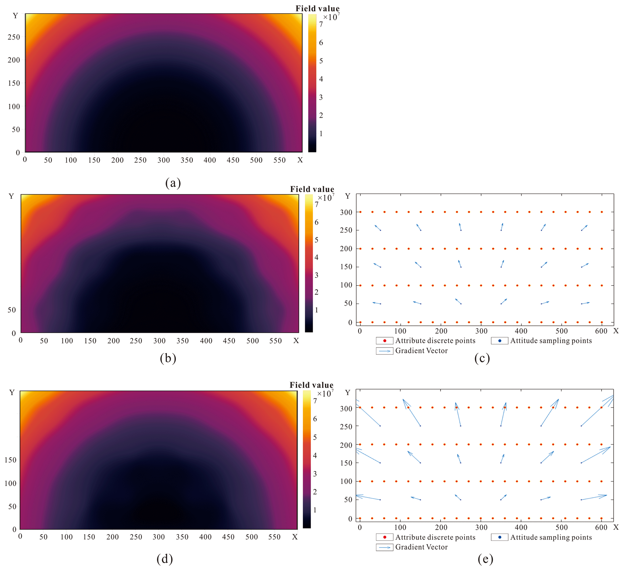
Figure 4 Experimental field 1: (a) original potential field, (b) field reconstructed when each gradient magnitude was set to a constant value of 1, (c) distribution of field attribute and unit gradient points, (d) field reconstructed when the gradient magnitude was obtained iteratively, and (e) distribution of field attribute and iteratively obtained gradient points.

In this study, we calculate the increment of λ from

$$\begin{array}{}\text{(12)}& {\mathit{\lambda }}_j^{t+\mathrm{1}}={\displaystyle \frac{a_{\mathrm{0}}}{\mathrm{1}+t}}+a_{\mathrm{1}}(l_j^t-l_j^{t-\mathrm{1}}{)}^{\mathrm{2}},\end{array}$$

where a₀ and a₁ are constant coefficients. We apply the same ${\mathit{\lambda }}_j^{t+\mathrm{1}}$ to three axes of x, y, and z. Given the updated ${\mathit{\lambda }}_j^{t+\mathrm{1}}$ and $l_j^t$, we substitute them into the (t+1)th HRBF system (Eq. 10) and solve for the updated coefficient of implicit function. This iterative process continues until the stopping criteria are satisfied.

We use two stopping criteria to finish the iterations. Firstly, for all observed strike and dip points, if the sum of differences in gradient magnitudes between two consecutive iterations is less than or equal to a small enough threshold ε, we stop the iterations when convergency is reached. Secondly, when the number of iterations reaches a given number N_iterate, we also obtain the final results of ${\mathit{\alpha }}_i^t$, ${\mathit{\beta }}_j^t$, and $l_j^t$.

$$\begin{array}{}\text{(13)}& \sum _{j=\mathrm{1}}^M\left|l_j^t-l_j^{t-\mathrm{1}}\right|\le \mathit{\epsilon },\end{array}$$

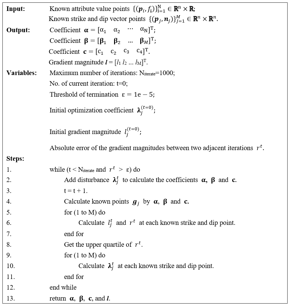
where $\left|\right|$ represents the absolute value of a real number, and M is the number of observed strike and dip points. The basic steps of the iterative calculation of gradient magnitude are given in the pseudo-code (Fig. 3).

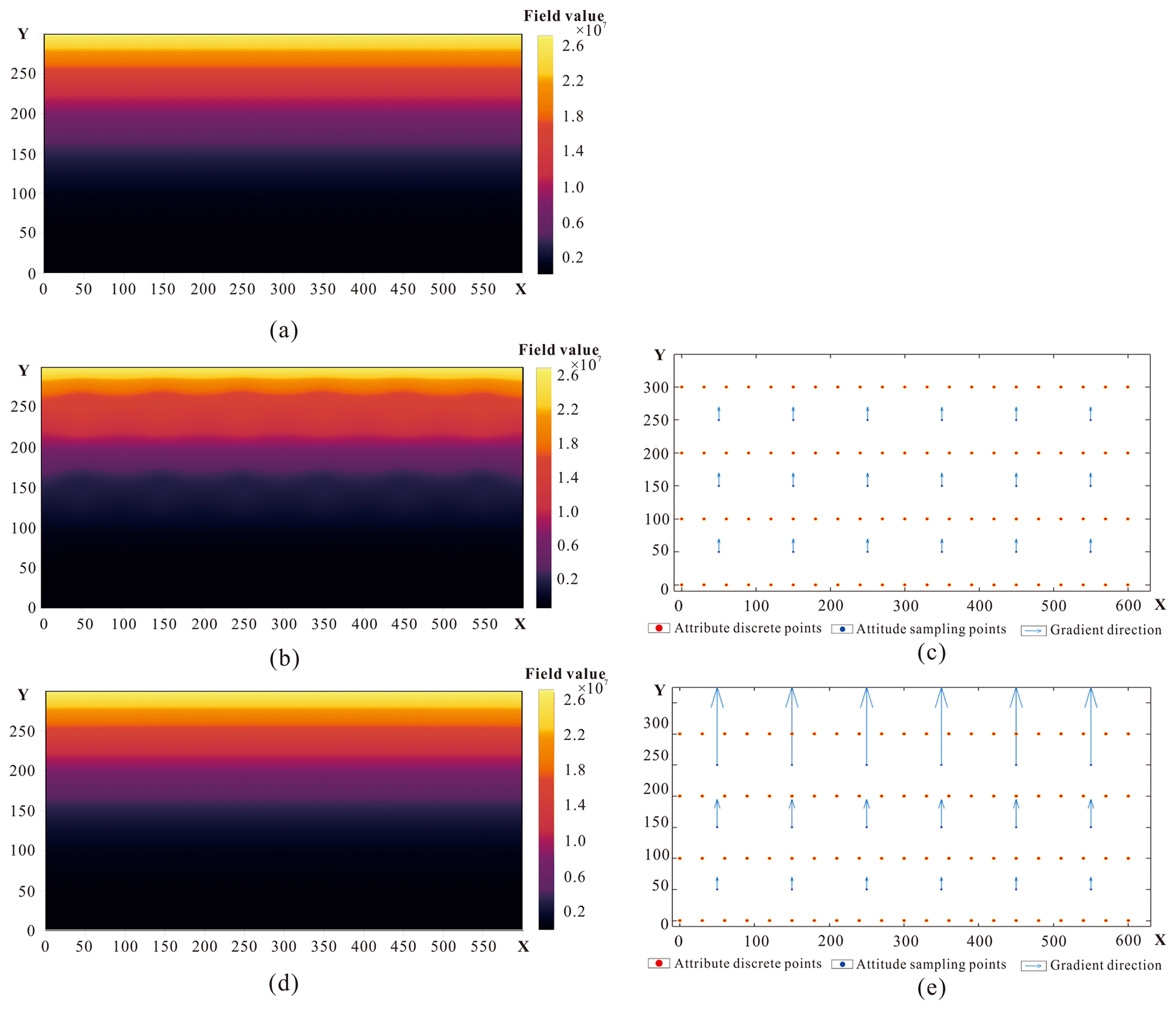
Figure 5 Experimental field 2: (a) original potential field, (b) field reconstructed when each gradient magnitude was set to a constant value of 1, (c) distribution of field attribute and unit gradient points, (d) field reconstructed when the gradient magnitude was obtained iteratively, and (e) distribution of field attribute and iteratively obtained gradient points.

4 Verification experiments

Two experimental fields in 2D space, with the gradient changing in direction or magnitude, were designed to verify the AdaHRBF method. The experimental results show that the different gradient magnitude settings apparently affect the modeled fields; moreover, the AdaHRBF method is effective to iteratively obtain the optimized gradient magnitude of the fields. We modeled an analytic field of $f_{\mathrm{1}}\left(\mathit{p}\right)=({\left({\mathit{p}}^x-\mathrm{300}\right)}^{\mathrm{2}}+{\left({\mathit{p}}^y\right)}^{\mathrm{2}}{)}^{\frac{\mathrm{3}}{\mathrm{2}}}$ with the changing gradient direction and magnitude, as shown in Fig. 4a. Then we sampled attribute and strike and dip points from the analytic field with different locations, as shown in Fig. 4b. Hence, we can retrieve the coefficients α_i and β_j of the HRBF formula and the polynomial coefficients, respectively. We compared two different experimental settings. (1) Assuming that the gradient is a unit vector, and each gradient magnitude is 1, we used the HRBF interpolant to reconstruct the field, as shown in Fig. 4c. Although the field values at the sampling points are equal to the given attribute values, the retrieved field values change irregularly; thus we obtained a large number of exceptional values in the reconstructed field. (2) The optimized gradient magnitude was obtained via the iterative AdaHRBF method introduced above. In this condition, we more accurately restored the field (as shown in Fig. 4d) and also got the optimized gradient magnitude after the iterations, which was close to the true value.

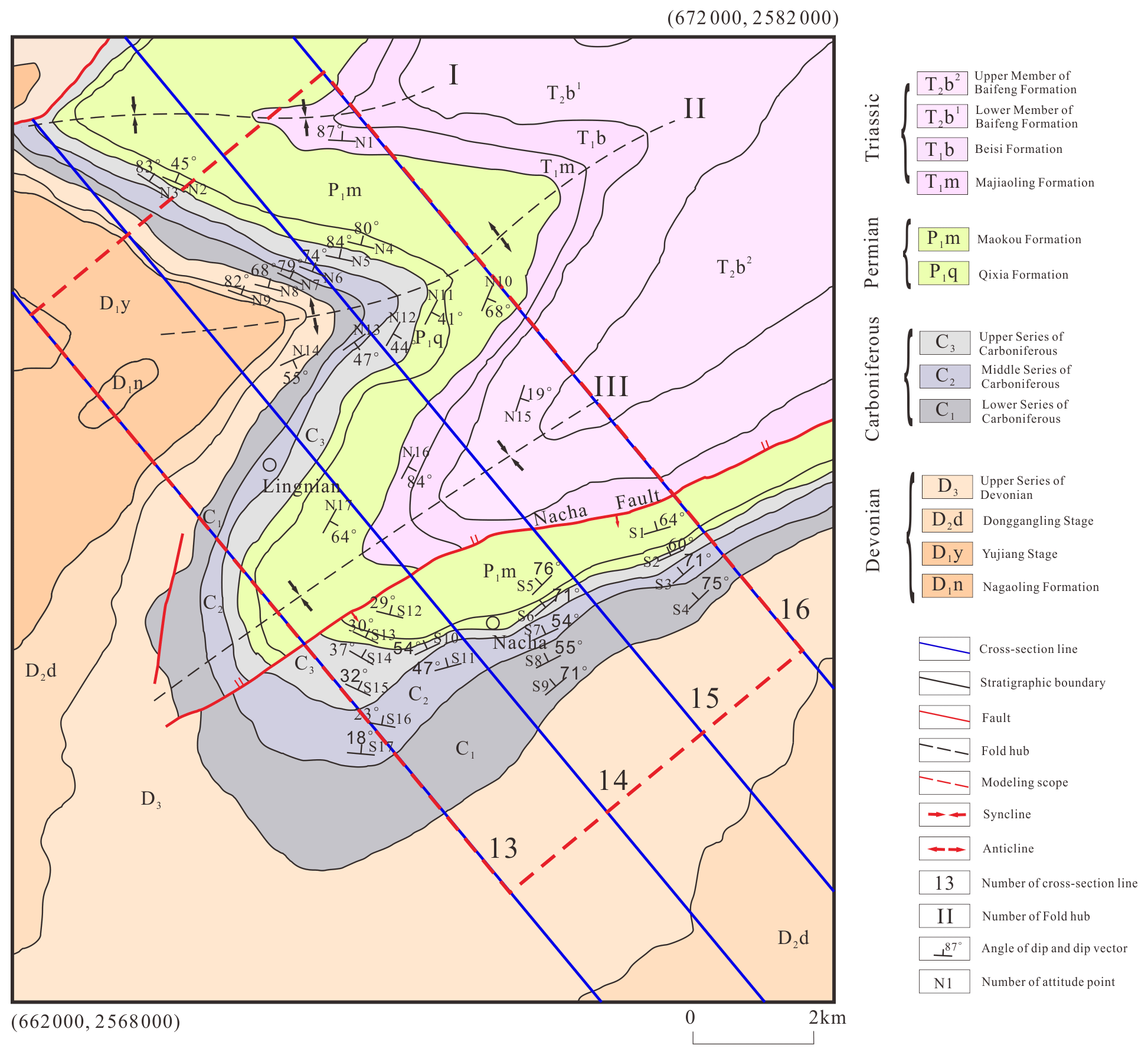
Figure 6 Geological map of the study area.

We also modeled a potential field of f₂(p)=(p^y)³ with the changing gradient magnitude, as shown in Fig. 5a. It is known that each direction of gradient points is the positive y-axis direction. We sampled attribute points and strike and dip points, as shown in Fig. 5b. We also compared two different experimental conditions: (1) assuming that each fixed gradient magnitude is 1, we used the HRBF interpolant to reconstruct the field, as shown in Fig. 5c, and (2) the optimized gradient magnitude was obtained via the iterative AdaHRBF method. In this condition, we more accurately restored the potential field (as shown in Fig. 5d) and also got the optimized gradient magnitude after the iterations.

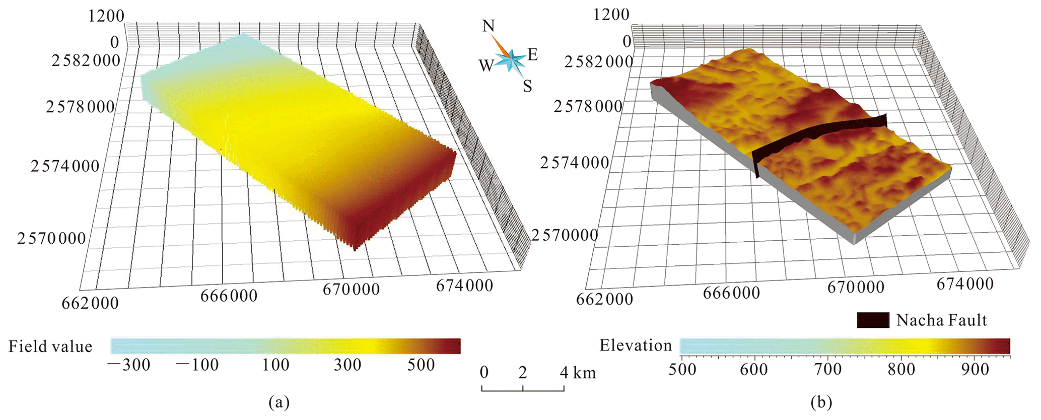
Figure 7 Model of Nacha Fault: (a) potential field and (b) surface model. We extracted the zero equipotential surface of the fault potential field (a) to reconstruct the surface model of the Nacha Fault, which divides the study area into two sub-domains (b). In each sub-domain, the coefficients of the HRBF linear system were separately solved according to the joint samplings of the SPF and its gradient.

5 Case study

5.1 Study area and dataset

The study area is located in the Lingnian–Ningping manganese ore zone, in Debao County, southwestern Guangxi Zhuang Autonomous Region, China (Fig. 6). The study area mainly consists of strata from the late Paleozoic to the late Triassic–Pliocene (T₃–N₂). The middle Permian (P₂) strata are in para-unconformity contact with early Triassic (T₁) strata; the middle Triassic (T₂) strata are in angular unconformity contact with the Quaternary. There is a left strike–slip inverse fault, the Nacha Fault, in the middle of the study area. It dips to the southeast, with a northeastern strike direction of 45^∘; a dip angle of about 70^∘; and a total length of about 12 km, extending outside the study area. The footwall slid to the west relative to the hanging wall, and the slip distance is about 600 m. There are two synclines (I and III) and an anticline (II) in the study area. Syncline III is located in the middle of the study area with a high symmetry. The axis of syncline III strikes nearly northeast, and its southern limb is cut by the Nacha Fault. Anticline II is located in the northwest of the study area with a good symmetry, the fold axis striking about 30^∘ northeast.

Faults, unconformable strata, and intrusive rocks all cause discontinuities in a SPF (Calcagno et al., 2008). We used the fault surface samplings to interpolate the potential field and extract the surface model of the Nacha Fault (Fig. 7).

According to the comprehensive stratigraphic column, the burial depth of each stratigraphic interface relative to the top surface of the Quaternary was used as the attribute value of the SPF (Fig. 8) for implicit-function interpolation. The SPF defines the 3D space as a scalar function f(p) at any point p, where f is defined as the relative burial depth in this study. Each point inside of a stratum has its own burial depth relative to the top surface of the Quaternary; therefore, the depth values in the field decrease gradually from bottom to top in strata. When the relative burial depth is used as the attribute value of the SPF, we can set the initial gradient magnitude ∥g∥≅1 if the strata underwent heterogenous deformation. However, if we use geological age as the attribute value of the SPF, ∥g∥ can no longer be initially assumed to be 1 because the stratigraphic age and distance along the gradient direction are from different measured variables.

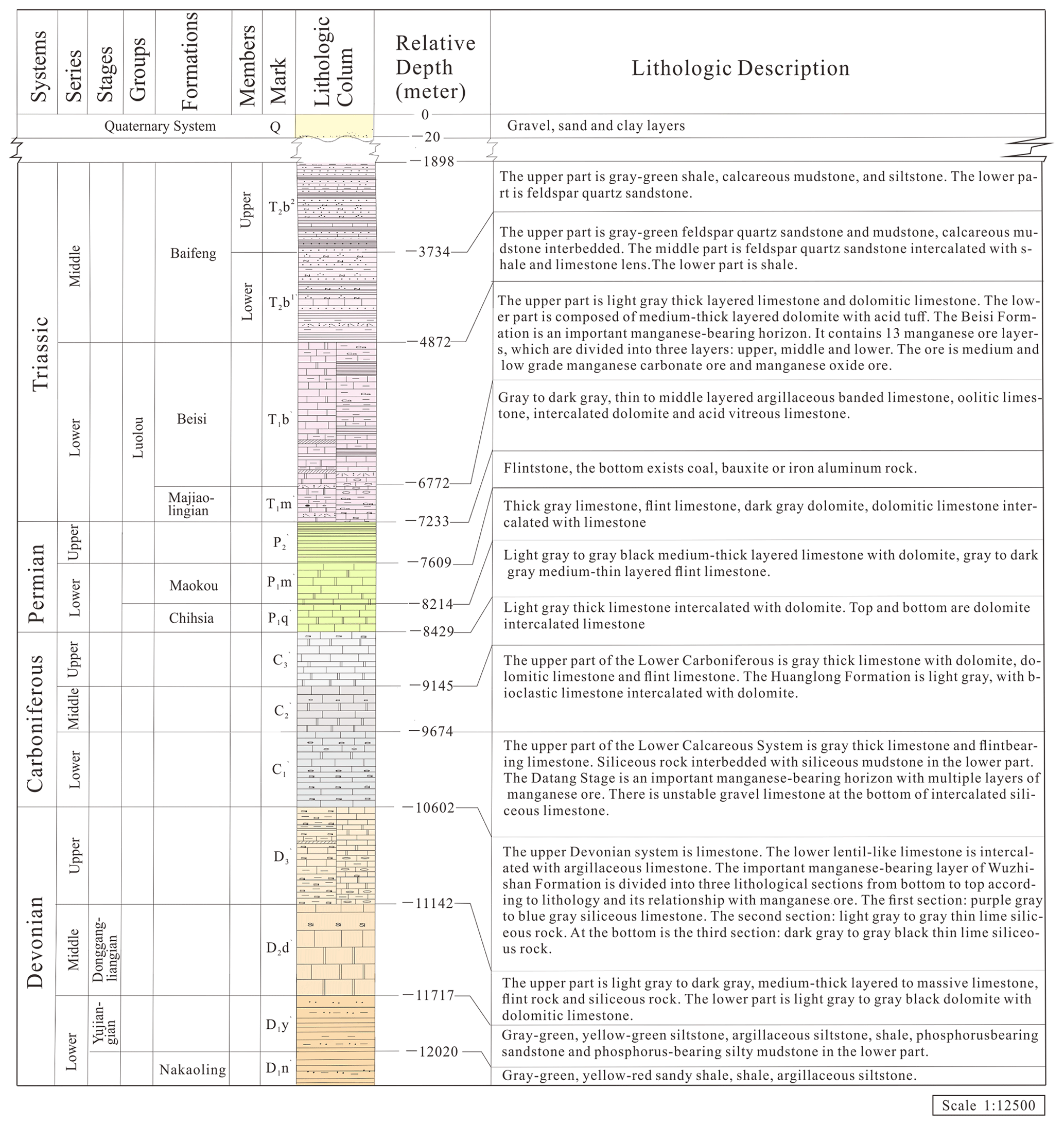
Figure 8 Comprehensive stratigraphic column of the study area. In this context, the SPF is fitted by a scalar function of the relative burial depth. Burial depth decreases as geological time progresses; therefore, earlier-deposited strata are assigned a relatively larger burial depth, while later-deposited strata are assigned a relatively smaller burial depth.

Based on the geological map and DEM of the study area, we produced a series of cross-sections (Fig. 9). However, the cross-sections were presented in 2D form. According to the necessary geographic projection parameters and scale, we derived the mapping relationship between 2D and 3D. Finally, we extracted the geological boundary points with 3D coordinates from 2D cross-sections.

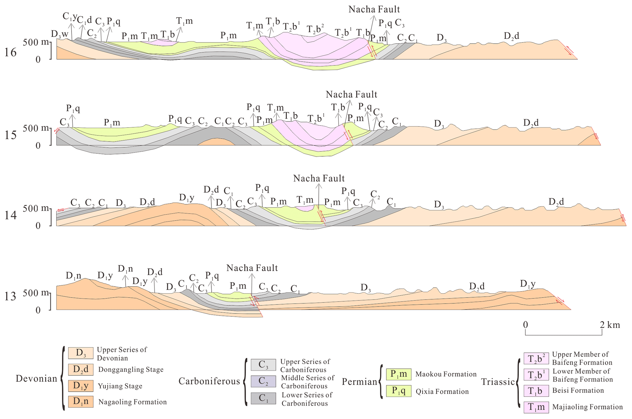
Figure 9 Geological cross-sections, mapped according to the planar geological map and DEM of study area. The cross-sections were mapped by vertical extension according to the boundaries and strike and dip points of strata along the layout lines of cross-sections.

The attribute points and strike and dip points of each stratigraphic interface and fault plane extracted from the geological map and cross-sections were used as the original dataset for 3D SPF modeling. The 3D points of stratigraphic interfaces extracted from the geological map and cross-sections were regarded as samplings of the SPF. The gradient vectors which are transformed from the off-contact stratigraphic strike and dip points were regarded as the samplings of the gradient of SPF.

5.2 Optimizing gradient magnitude

There are 1410 known on-contact attribute points and 34 off-contact strike and dip points scattered throughout the study area (Fig. 10a). The known strike and dip sampling points are scattered on the southern limb of fold I, the northern and southern limbs of fold II, and the northern and southern limbs of fold III. There are 17 strike and dip sampling points on the northern side of the Nacha Fault and 17 strike and dip sampling points on the southern side. The distribution of the dip directions and dip angles is shown in Fig. 10b.

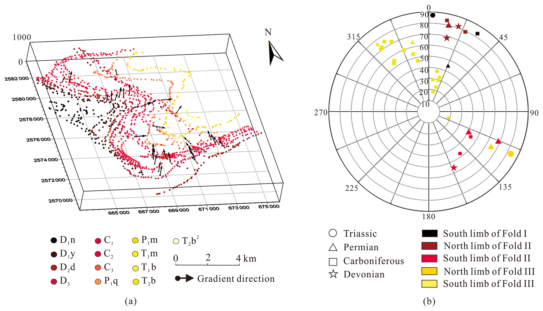
Figure 10 Scattered attribute points and strike and dip points of strata: (a) known attribute points and strike and dip points of strata and (b) distribution of the dip directions and dip angles of the strike and dip points, in which the symbols represent different strata, and the colors represent different limbs of folds.

First, we set the initial gradient magnitude to 1.0 and calculated the x-, y-, and z-axis components of the gradient vector field according to the dip direction and angle of the strike and dip points. We constructed HRBF solution matrices on the northern and southern side of the Nacha Fault, respectively. Then, we iterated to converge toward the optimized gradient magnitudes by adding an optimization term to the HRBF linear system. The termination conditions were met after 200 iterations in the northern sub-domain and 300 iterations in the southern sub-domain. The gradient magnitudes became stable, and finally the optimized magnitudes of the gradient were obtained. The changes in gradient magnitude are shown in Fig. 11.

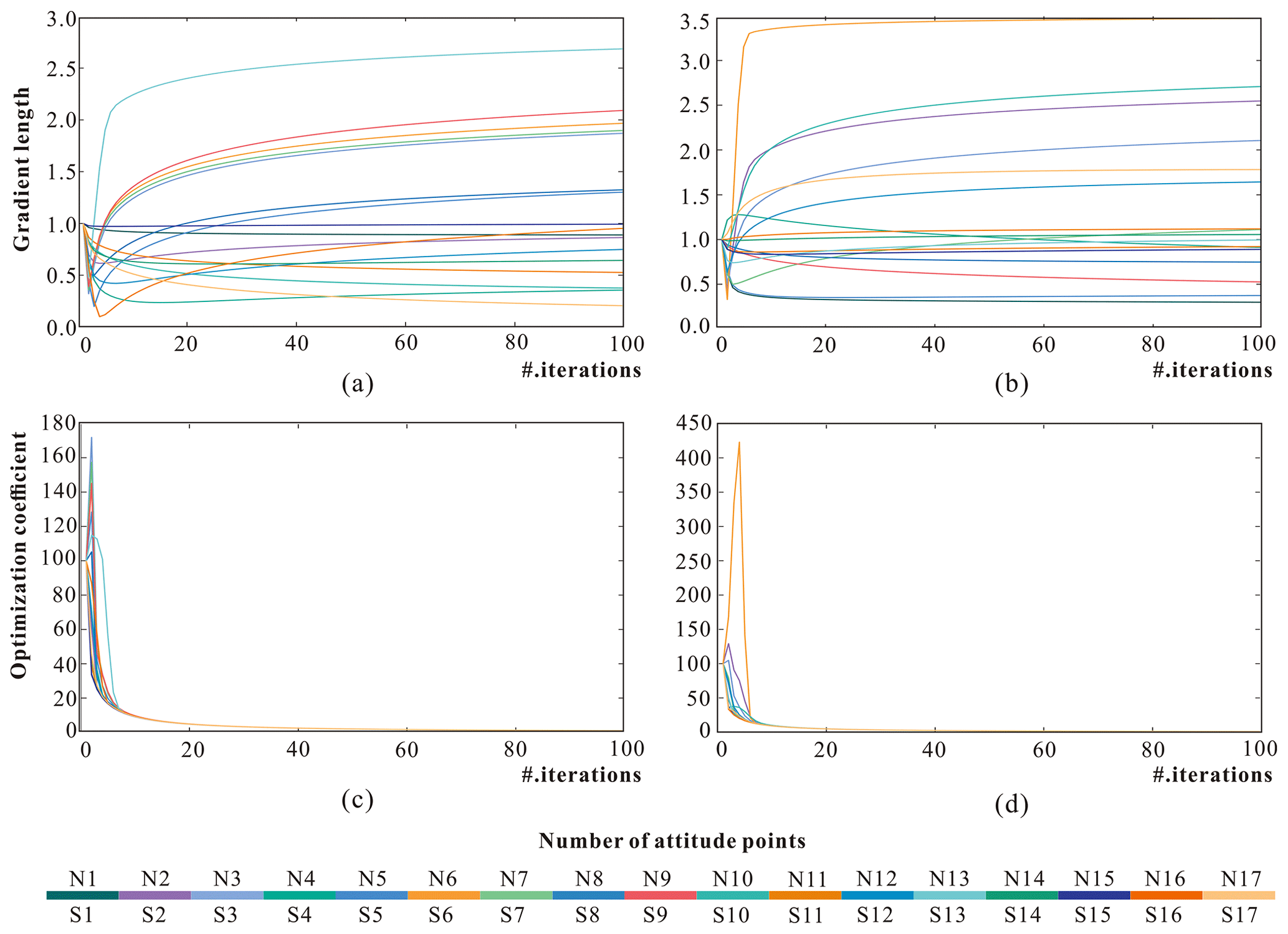
Figure 11 Changes in optimization coefficient λ and gradient magnitude: (a) gradient magnitudes for all strike and dip points in the northern sub-domain, (b) gradient magnitudes for all strike and dip points in the southern sub-domain, (c) optimization coefficients for all strike and dip points in the northern sub-domain, and (d) optimization coefficients for all strike and dip points in the southern sub-domain. The corresponding number of strike and dip points can be found in Fig. 6.

On a specific grid resolution, we modeled the scalar field of gradient magnitude before and after optimization for each strike and dip point (Fig. 12). Furthermore, we cut four cross-sections of the gradient magnitude scalar field, as shown in Fig. 13.

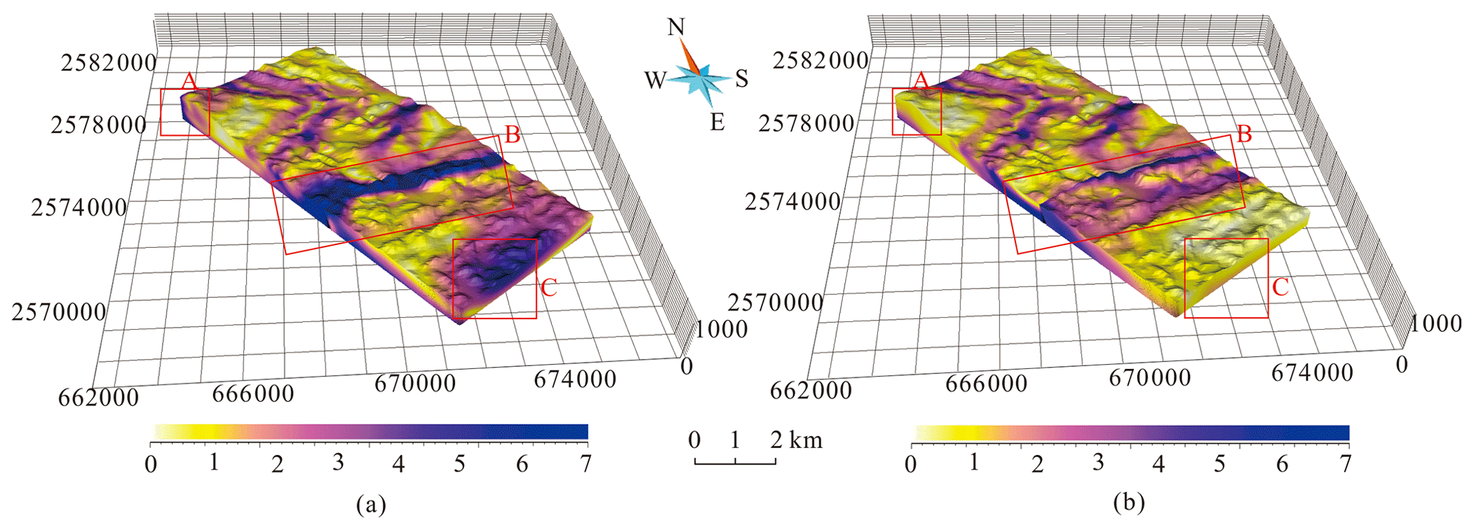
Figure 12 Scalar field of (a) gradient magnitude assigning an initial fixed gradient magnitude of 1 for each strike and dip point and (b) gradient magnitude after optimization. Along the northern side of the Nacha Fault in (a), the gradient magnitudes obtained by interpolation in area B exceed the maximum values. Compared with the scalar field of gradient magnitude before optimization, the scalar field of gradient magnitude after optimization (b) more smoothly represents changes in the strata. The Carboniferous strata have the largest optimized gradient magnitude, while the optimized gradient magnitudes of the Devonian strata are smallest.

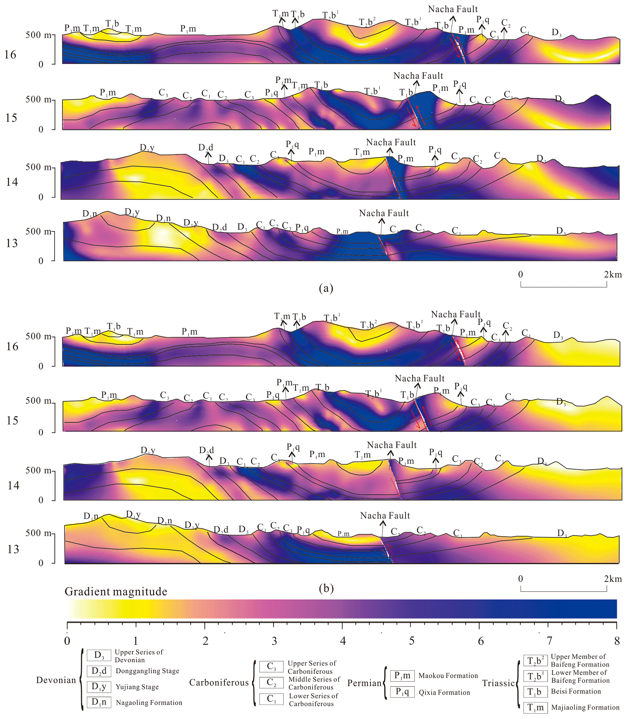
Figure 13 Cross-sections of the gradient magnitude field: (a) assigning an initial fixed gradient magnitude of 1 for each strike and dip point and (b) after optimization.

5.3 Stratigraphic potential field (SPF)

After the optimized gradient magnitude for each strike and dip point was obtained, all scattered attribute points and strike and dip points were finally substituted into the HRBF linear system to respectively solve the HRBF coefficients (α_i, β_j) and the polynomial coefficients (c₁c₂c₃c₄) for each side of the Nacha Fault. On a specific grid resolution, we generated the regular discrete grids as interpolated points in 3D space. Then the points above the digital elevation model (DEM) were removed from the interpolated points. Finally, we reconstruct the SPFs in 3D space before and after optimization of the gradient magnitude according to the respective HRBF interpolant of each sub-domain. In this study, the SPF represents the relative burial depth in 3D space. The larger field value represents earlier-deposited strata with larger relative burial depth, and vice versa. The same stratigraphic interfaces in different sub-domains share the same field value. The field values change abruptly at the Nacha Fault because the conformable strata were cut by the fault plane.

The SPFs are both constrained so that the interpolated SPF values at the attribute points are equal to the initial relative burial depths, but the SPF values may abruptly change or produce outliers at some locations. Obviously, the SPF values change nonuniformly with gradient magnitude before optimization (Fig. 14a), which caused the SPF values that originally belonged to the Carboniferous strata to be interpolated as those of other strata and sequentially resulted in incorrect extraction of the stratigraphic interfaces. This nonuniform gradient change in stratigraphic potential field causes separated, discontinuous, and dispersed stratigraphic interfaces to be extracted through equipotential surface tracking. However, reconstructing the SPF through optimization of gradient magnitude for each strike and dip point (Fig. 14b) avoids the generation of either abnormal field values or of the wrong equipotential surfaces. This geologically plausible SPF can be appropriately constrained by the known gradient direction and the optimized gradient magnitude at the strike and dip sampling points.

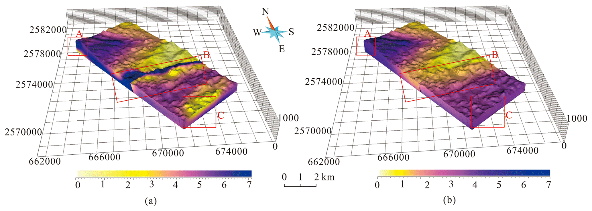
Figure 14 Stratigraphic potential field (a) before and (b) after optimization of gradient magnitude. The abnormal SPF values (areas A, B, and C in panel a) are not continuously distributed along stratigraphic interfaces but appear at irregular intervals.

We cut the SPF along four section lines, and the SPF value also changes more uniformly from older to younger strata after gradient magnitude optimization than using a fixed gradient magnitude of 1, as shown in Fig. 15.

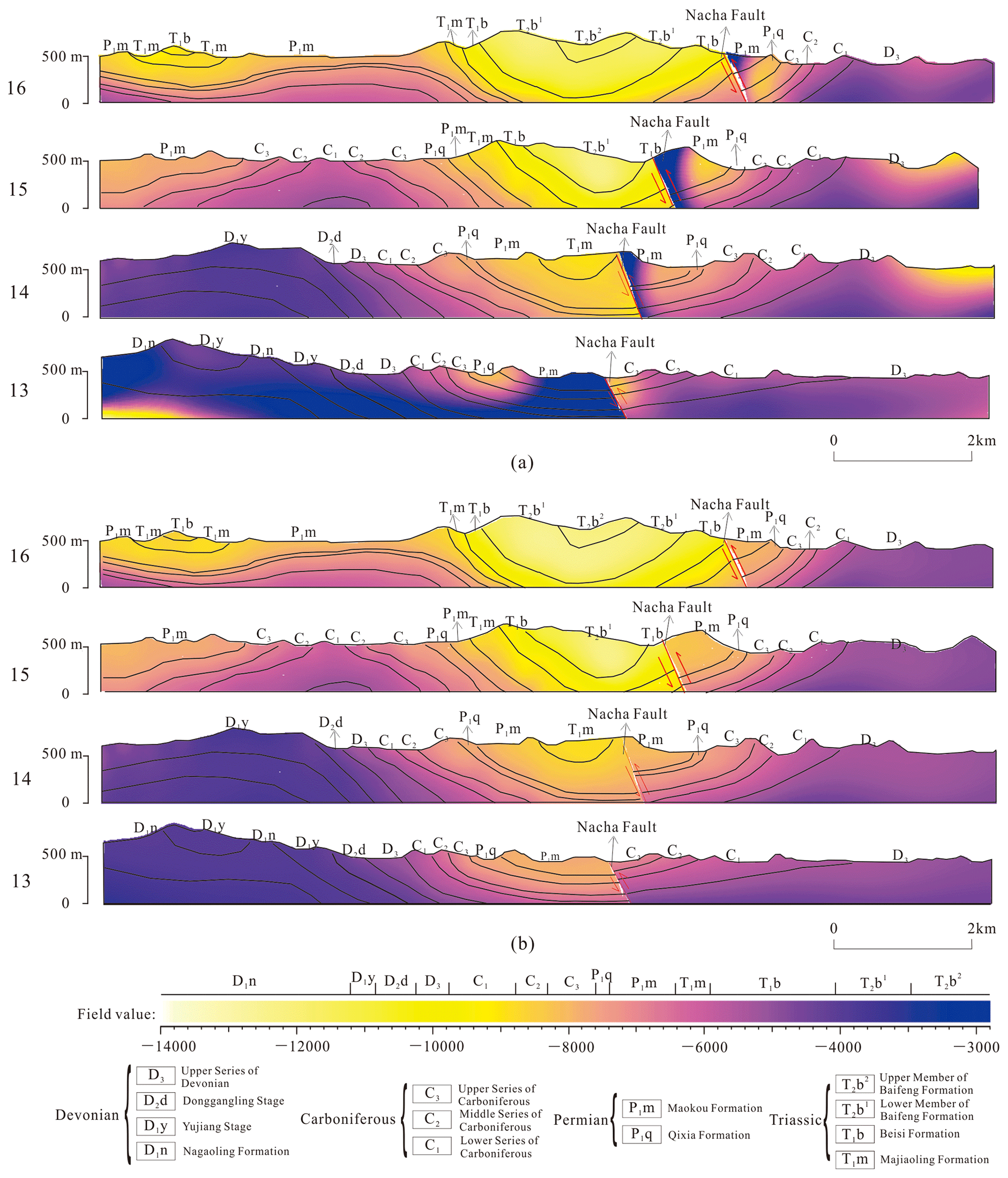
Figure 15 Cross-sections of the stratigraphic potential field (a) before and (b) after optimization of gradient magnitude.

5.4 Three-dimensional models of strata

Once the field was interpolated in 3D space, the specific equipotential surfaces were extracted from the implicit volumetric function as stratigraphic interfaces within each main-structure-bounded sub-domain. We used the marching cube method to extract the equipotential surfaces with a specific relative burial depth from the stratigraphic interfaces by connecting all the points with the same field value in the stratigraphic potential field (Fig. 16). The interface model on both sides of the Nacha Fault restores the location of the fault in the southern limb of syncline III.

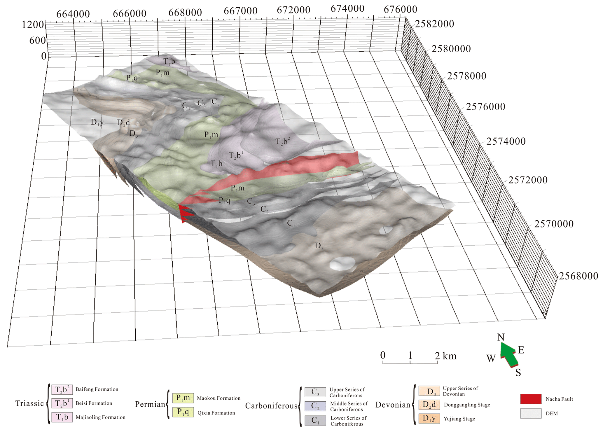
Figure 16 Three-dimensional model of the bottom surfaces of strata. The 3D surface model extracted from the potential field shows that the geometrical shape of each equipotential (iso-depth) surface is smooth, and the topology is consistent.

Sequentially, according to the range of relative burial depth of stratigraphic top and bottom, two solid stratigraphic models were reconstructed from these equipotential surfaces before and after optimization of gradient magnitude for each strike and dip point, respectively, combined with sub-domain boundaries and the DEM (Fig. 17). The HRBF interpolation with the initial fixed gradient magnitude of 1 roughly reflects stratigraphic on-contact information and captures the structure of syncline I in the north. However, several details are different from the stratigraphic structure on the geological map. Where the Nacha Fault passes through syncline III, the strata on the southern side of the fault plane should correspond to the same strata on the northern side. However, the Devonian strata corresponded to the Permian strata in area B, as shown in Fig. 17a and b, which is inconsistent with the geological structure. The geological model extracted using the optimized gradient magnitude for each strike and dip point is shown in Fig. 17c. Overall, the obtained geometries follow the shape of the folds and stratigraphic on-contact lines more closely. From north to south in the study area, anticline II and syncline III were successfully modeled with the Nacha Fault correctly represented as an inverse fault that cuts syncline III. On both sides of the Nacha Fault, the sequence of the strata is the same, and the model exhibits traces of the fault plane passing through the stratigraphic surfaces.

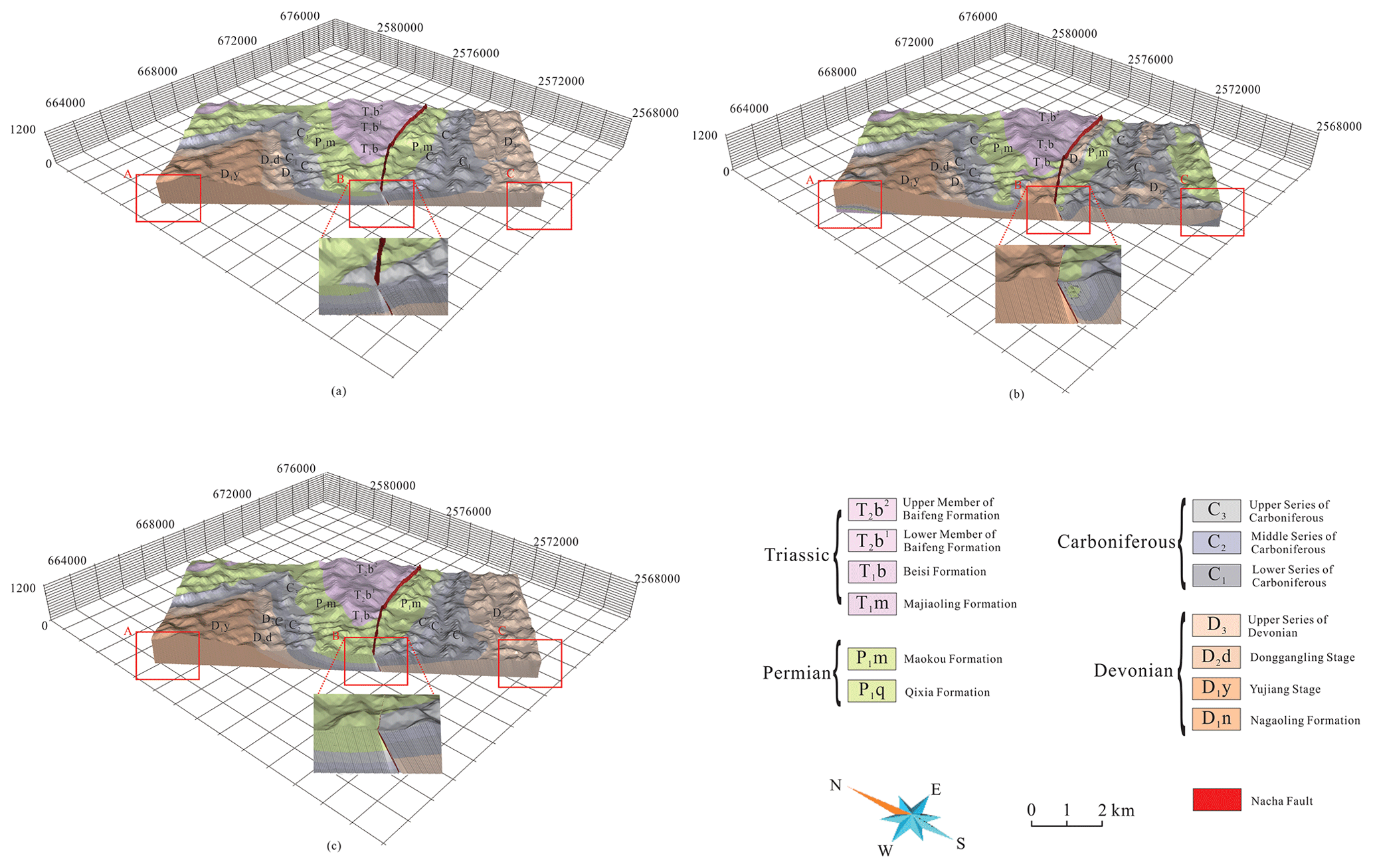
Figure 17 Three-dimensional stratigraphic models using (a) RBF without gradient constraint, (b) HRBF with unit gradient, and (c) AdaHRBF with optimized gradient magnitude. Many abnormal potential-field values and additional unreasonable geological bodies were extracted from the model before optimization, especially in areas A, B, and C, as shown in (a) and (b). These abnormal potential-field values lead to the occurrences of additional strata fragments that do not conform to the rule of sediments.

Four cross-sections through the solid models (see the geological map for cross-section lines) were cut, and the cross-sections of the solid model are more consistent with the original structural relationships on the geological map after gradient magnitude optimization than using HRBF with a fixed gradient magnitude of 1 and RBF without gradient constraint, as shown in Fig. 18.

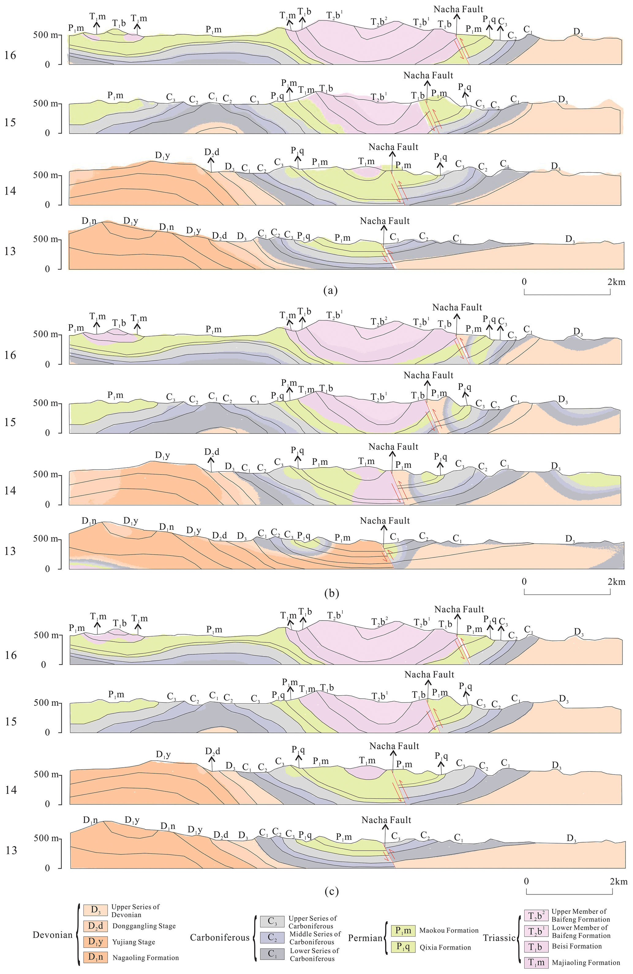
Figure 18 Cross-sections of the solid models. (a) RBF without gradient constraint, (b) HRBF with unit gradient, and (c) AdaHRBF with optimized gradient magnitude.

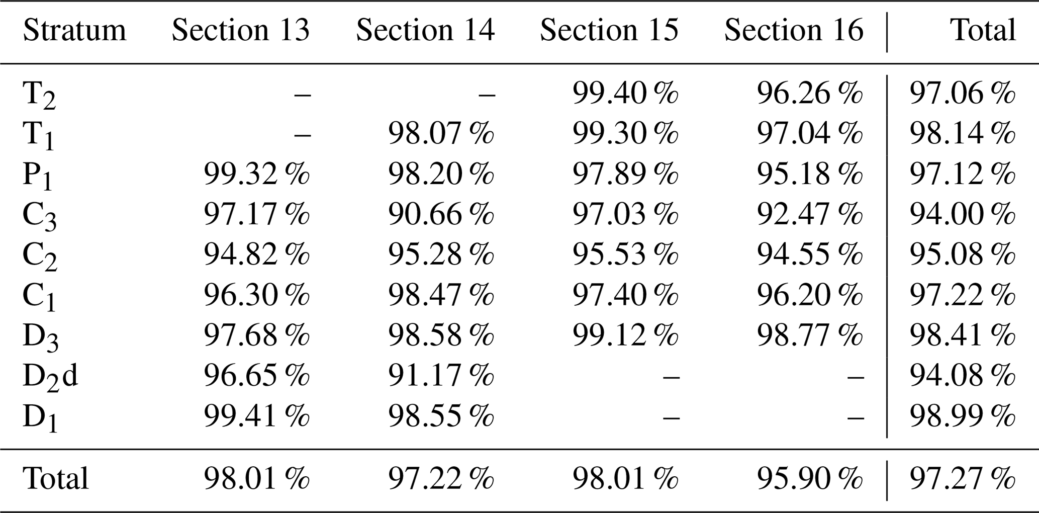
The highest stratum and section coincidence percentages on cross-sections are 74.50 % (T₂) and 78.03 % (Section 16) before optimization, respectively, as shown in Table 1. However, the highest stratum and section coincidence percentages on cross-sections are 98.99 % (D₁) and 98.01 % (Sections 13 and 15) using the optimized gradient magnitude for each strike and dip point, respectively, as shown in Table 2. The total coincidence percentage on cross-sections increases from 67.03 % to 98.27 % after optimizing the gradient magnitude.

Table 1 Coincidence percentages on cross-sections using RBF without gradient constraint.

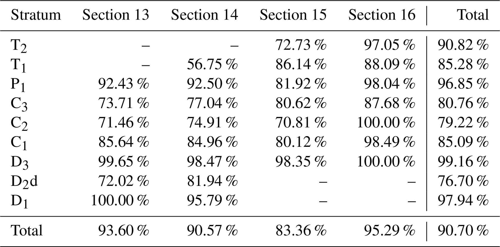
Table 2 Coincidence percentages on cross-sections using HRBF with an initial fixed gradient magnitude of 1 for each strike and dip point.

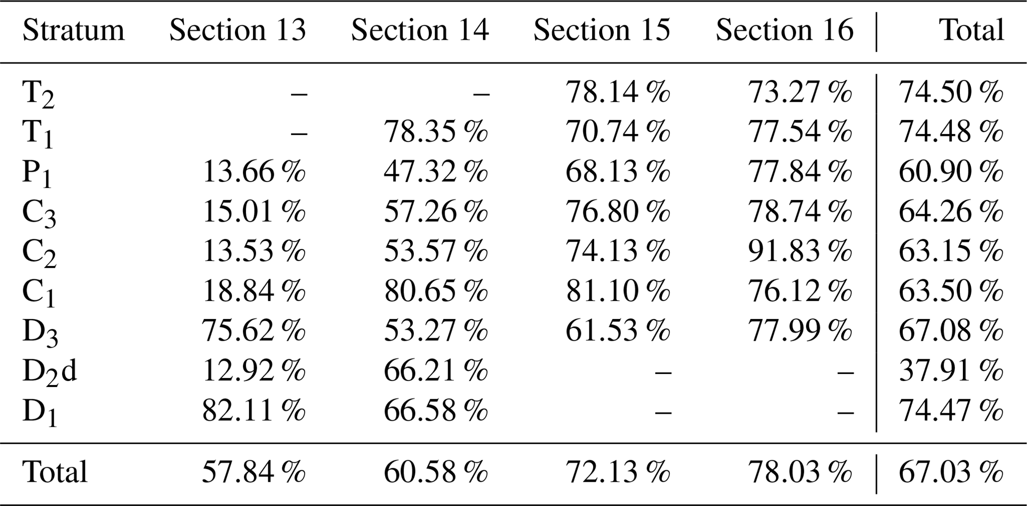
Table 3 Coincidence percentages on cross-sections using AdaHRBF with optimized gradient magnitude.

6 Discussions

The AdaHRBF proposed in this study improves the use of strike and dip data in SPF modeling by optimization of gradient magnitudes. In addition to use of strike and dip information as the gradient directions of SPFs, we use the gradient magnitude as a new constraint to control the rate of change in SPF values. The gradient of a SPF is a vector with certain direction and magnitude, in which the gradient magnitude provides constraints on the thickness of deformed strata. Therefore, it is extremely important to construct HRBF linear systems with accurate gradient magnitudes in 3D SPF modeling. As a “chicken-and-egg” problem, it is difficult to determine the exact gradient magnitude through the geological measurements or prior structural knowledge. We proposed an iterative optimization method which alternates between estimation of SPF and gradient magnitudes so that the gradient magnitudes progressively converge towards the values and are adaptive to the stratigraphic architecture. The optimized gradient magnitudes more accurately simulate the variations in the SPF between the top and bottom surfaces. Besides constraints of scattered multivariate Hermite–Birkhoff data, the generalized RBF (Hillier et al., 2014) reconstructs an implicit function with more constraints of lithologic markers (inequality) and lineations (tangent). How to integrate these constraints in our solution to utilize more kinds of modeling data shall be studied in future work.

Jessell et al. (2014) highlighted two limitations of current implicit modeling schemes: (1) they are incapable of interpolating or extrapolating a fold series within a continuous structural style; (2) the shape of fold hinges they produce is not controlled and may yield inconsistent geometries. To overcome these two limitations, we adopted two strategies: (1) a 3D stratigraphic-potential-field modeling method based on HRBF interpolants was used to interpolate a fold series within a structurally continuous domain; (2) a number of structural strike and dip points were sampled on both limbs of the folds to control the geometries of fold hinges. A novel method for modeling folds uses a fold coordinate system based on fold axis direction, fold axial surface, and extension direction and incorporates a parametric description of fold geometry (e.g., fold wavelength, amplitude, tightness, and rotation angle) into the interpolation algorithm (Laurent et al., 2016; Grose et al., 2017, 2019), which would be our future research direction of fine fold modeling based on AdaHRBF.

There are several choices for the value of the potential field, e.g., the sorted serial number, burial depth, or depositional time for each stratigraphic interface (Mallet, 2004). However, the thickness of the stratum is not necessarily proportional to the sorted serial number and deposition time. Compared with using the sorted serial number or depositional age of stratigraphic interfaces as the potential-field value, choosing the burial depth is more in line with 3D SPF modeling. We derived the gradient direction from the strike and dip points; moreover, we used the gradient magnitude as a constraint to control the rate of change in the SPF.

7 Conclusions

The purpose of this study is to establish a framework for 3D SPF modeling by using the HRBF interpolant with adaptive gradient optimization constrained by on-contact attribute points and off-contact structural strike and dip points. We applied this method to a study site in the Lingnian–Ningping area, and a geological map, four cross-sections, and a DEM were used as original data to model a SPF whose field value was taken from the relative burial depth of the stratigraphic interfaces. The results show that the implicit modeling of the SPF by HRBF interpolants and optimization of gradient magnitude can be effectively adapted to 3D geological modeling using the sampling points from a geological map and cross-sections. A SPF can express the parameters of a stratum such as property, shape, and topology in 3D space.

However, the modeling process is complicated because the sub-domains are required to be divided manually. In actual geological surveys, the geological structure may be more complex and include a large number of faults, unconformable strata, and intrusive rocks. Therefore, it is necessary to separately identify the boundary of the sub-domains according to the fault interfaces, unconformable strata, and intrusive rocks before the 3D geological modeling work. A goal for future work is to introduce a way to integrate faults (Grose et al., 2021a) into the implicit model to accommodate discontinuity of fault planes. In addition, the 3D orientations are usually surveyed on the outcrop strata; however, it would introduce uncertainty if we were to assume that the orientations of a totally subsurface terrain are consistent with its conformable outcrop strata. Therefore, this uncertainty in the model should be considered in the modeling process, and additional geophysical exploration data and geological interpretation should be incorporated into the modeling constraints.