PySubdiv 1.0: open-source geological modeling and reconstruction by non-manifold subdivision surfaces

Sealed geological models are commonly used as an input to process simulations, for example, in hydrogeological or geomechanical studies. Creating these meshes often requires tedious manual work, and it is therefore difficult to adjust a once-created model. In this work, we propose a flexible framework to create and interact with geological models using explicit surface representations. The essence of the work lies in the determination of the control mesh and the definition of semi-sharp-crease values, which, in combination, enable the representation of complex structural settings with a low number of control points. We achieve this flexibility through the adaptation of recent algorithms from the field of computer graphics to the specific requirements of geological modeling, specifically the representation of non-manifold topologies and sharp features. We combine the method with a particle swarm optimization (PSO) approach to enable the automatic optimization of vertex position and crease sharpness values. The result of this work is implemented in an open-source software (PySubdiv) for reconstructing geological structures while resulting in a model which is (1) sealed/watertight, (2) controllable with a control mesh and (3) topologically similar to the input geological structure. Also, the reconstructed model may include a lower number of vertices compared to the input geological structure, which results in reducing the cost of modeling and simulation. In addition to enabling a manual adjustment of sealed geological models, the algorithm also provides a method for the integration of explicit surface representations in inverse frameworks and the consideration of uncertainties.

1 Introduction

Parametric surface-based representation is one of the major approaches to the surface representation of geological objects (De Kemp, 1999; De Paor, 1996; Farin and Hamann, 1997). Several studies considered a surface-based approach in geological modeling since the outstanding features of the structure, e.g., heterogeneity, are explicitly demonstrated by the surfaces of the boundary without depending on grid cells (Moulaeifard et al., 2023; Jacquemyn et al., 2019). It is worth mentioning that Jacquemyn et al. (2019) comprehensively investigate the advantages of surface-based modeling compared to grid-based representation. Botsch et al. (2010) consider NURBS (non-uniform rational B splines) and subdivision surfaces as two major methods of parametric surface-based representation for generating controllable free-form surfaces. Subdivision surfaces convert an initial mesh (control mesh) to a smooth mesh by successive refinements until the final mesh is sufficiently fine. The final smooth mesh is a controllable free-form surface which can be controlled easily by the control points (vertices of the initial mesh). Although both NURBS and subdivision surfaces produce controllable free-form surfaces, subdivision surfaces give freedom from topological limitations, whereas NURBS underscores the smooth manipulation of the model (Cashman, 2010).

Previous studies of geological modeling have dealt with NURBS (Börner et al., 2015; Jacquemyn et al., 2019; Paluszny et al., 2007). However, NURBS surfaces suffer from two limitations: (1) for generating a model with complex topology, several NURBS patches have to be stitched together, which leads to difficulty in modeling, and (2) modification of NURBS surfaces is challenging in the complex cases since NURBS surfaces are based on grid structures (Botsch et al., 2010; DeRose et al., 1998; Sederberg et al., 2008).

Although extensive research has been carried out on exploiting NURBS for geological and reservoir modeling, researchers have not considered subdivision surfaces in much detail. Lévy and Mallet (1999) and Mallet (2002) investigate the subdivision surface method, which exploits discrete smooth interpolation (DSI) as the refinement scheme at each iteration. In their approach, all vertices (except the control vertices) are free to move in each iteration since DSI is a discrete fairing method. Although their work deserves appreciation, they mention that the formal proof of the convergence of the series of recursively refined meshes is an open question; however, it can be observed experimentally. Also, they do not investigate the compatibility of subdivision surfaces for the structures with non-manifold topologies, which is broadly observed in complex geological and reservoir modeling, e.g., connection between faults and horizons, channel intersection and hierarchically layered structures. In this paper, we focus on the non-manifold subdivision surface method based on the Loop algorithm, in which the convergence of the series of refined meshes is formally proved (Loop, 1987).

One of the typical examples of non-manifold surfaces in geological modeling is where several faces of the mesh share one edge (Fig. 1). Representations of non-manifold structures require complex algorithms (Rossignac and Cardoze, 1999). The lack of supporting non-manifold surfaces is one of the limitations of classical subdivision surfaces. Ying and Zorin (2001) modified the subdivision surface algorithm and made it compatible with the non-manifold topology which is implemented in the core of PySubdiv.

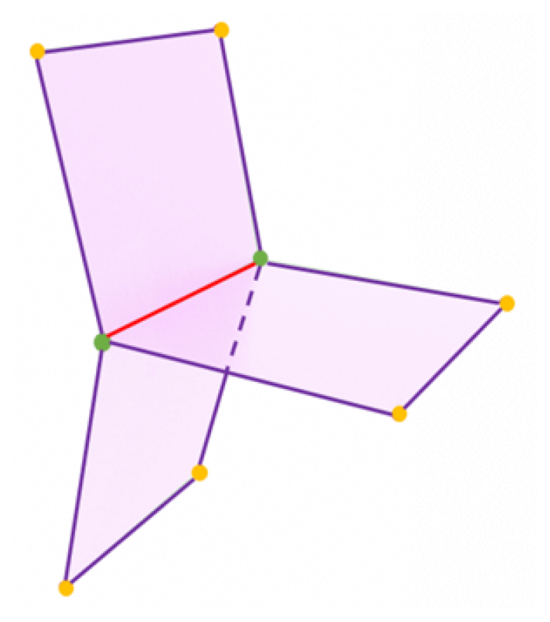
Figure 1 A common example of a non-manifold topology in geological modeling; multiple faces share one edge. Non-manifold vertices (green) and edge (red).

Classic subdivision surface algorithms tend to generate smooth surfaces. However, complex geological structures inherently consist of creases and corners (e.g., sharp fault bend), which require modified subdivision algorithms. Subdivision surfaces with the semi-sharp-crease approach generate creases on the mesh by increasing the resistance of the vertices to the smoothing procedure. In practice, the resistance of the vertices can be created by applying the crease sharpness value to the edges consisting of the respective vertices. The higher the crease sharpness value of the edge is, the sharper the creases on the structure. It is worth mentioning that PySubdiv exploits the semi-sharp creases for a better representation of the creases of complex geological structures.

Furthermore, the subdivision surfaces are used for reconstruction by fitting smooth surfaces to mesh or dense point cloud data (Ma et al., 2015). The goal of reconstruction in this paper is to generate the control mesh that gives control over the reconstructed mesh with few control points. In other words, the reconstructed mesh not only is fitted to the input mesh but also can be controlled by vertices of the control mesh. Moulaeifard et al. (2023) investigate the reconstruction of geological structures by non-manifold subdivision surfaces. However, they manually fit the smooth surfaces to the input data, which is a time-consuming process in complex geological structures. This paper presents the automatic reconstruction of geological structures which is implemented in the PySubdiv.

The structure of the control mesh is based on two critical variables: (1) the position of the control points and (2) the crease sharpness value of each edge. Therefore, for fitting the smooth mesh to input data, the position of the control points and crease sharpness values have to be set. Several researchers have studied the simplification method to estimate the control mesh from the input mesh (Hoppe et al., 1994; Suzuki et al., 1999; Wu et al., 2017). However, Ma et al. (2015) advise exploitation of the distinguished features of the input mesh instead of the simplification method since simplification would be time-consuming for structures with complex topology. It is worth mentioning that extensive research has been carried out on exploiting the key features of the input mesh for generating the control mesh; Ma et al. (2015) use the umbilics and ridges. Also, Marinov and Kobbelt (2005) and Kälberer et al. (2007) consider the curvatures for generating the control mesh.

After estimating the control mesh, we have to optimize the control mesh to find the best fit to input mesh. Wu et al. (2017) investigate automatic fitting to solve the optimization problem by using the augmented Lagrangian method. They show that their method provides significant gains over previous works, e.g., Marinov and Kobbelt (2005), by generating the reconstructed mesh with fewer control points while consisting of comparable errors. Therefore, for the sake of efficiency, PySubdiv makes use of the automatic reconstruction method proposed by Wu et al. (2017), which is explained in Sect. 2.4. The final reconstructed structure is controllable by control points, sealed (or watertight) and topologically similar to the input model.

To date, there is no practical software to generate and manipulate sealed geological models using subdivision surface approaches. We attempt to close this gap with the approach described in this paper and the implementation in the accompanying software package PySubdiv. This study investigates the advantages and limitations of PySubdiv for the modeling and reconstruction of geological and reservoir structures with a case study. Also, PySubdiv can export the final files as 3D objects based on common object formats, e.g., obj, which can be read by most computer graphics and meshing software.

2 Methods

The core functionality of PySubdiv consists of four fundamental parts, which are investigated in the following section: (1) subdivision surface algorithm, (2) modeling with semi-sharp creases, (3) supporting non-manifold topology and (4) automatic reconstruction.

2.1 Subdivision surface algorithm

The subdivision surface algorithm refines the input (control) mesh to generate the final desirable mesh based on mathematical rules (Peters, 2015; Halstead et al., 1993; Stam, 1998; Reif, 1995). Subdivision surfaces follow two steps at each refinement: (1) the splitting step, which includes implementing the new vertices on the surface, and (2) the averaging step for updating the location of the vertices. There are several subdivision surface schemes based on different criteria, e.g., type of input mesh (triangular or quad) and the approach for refinement. The Loop scheme (Loop, 1987) is one of the common subdivision schemes for triangular meshes and is already implemented in PySubdiv. In the following, the Loop algorithm is explained.

2.1.1 Loop subdivision scheme

Loop (1987) defines the Loop algorithm to generate smooth surfaces for triangular meshes by using splitting and averaging steps in each refinement stage. In the splitting step, a new vertex is inserted on the midpoint of each edge (blue vertex in Fig. 2), which results in the splitting of each triangle of the control mesh into four triangles.

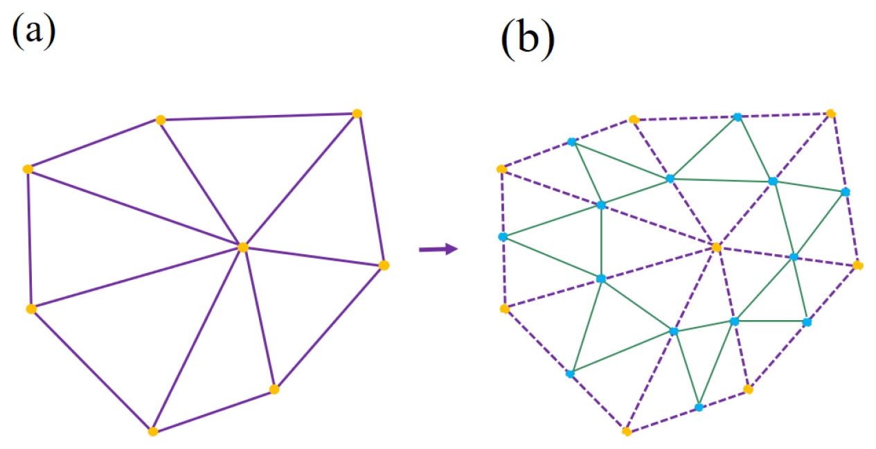
Figure 2 Splitting step of Loop scheme. (a) The control mesh. (b) Splitting each triangle into four by inserting new vertices (yellow vertices) in the middle of each edge.

Updating the position of the existing and midpoint vertices (yellow and blue vertices) is the averaging step of the Loop scheme (Fig. 3). To determine the new position of the existing vertex (q) with m adjunct vertices (r₁, r₂, r₃, …, r_k) the Loop scheme proposes (Fig. 3a)

$$\begin{array}{}\text{(1)}& q_{\mathrm{new}}=q\cdot \left(\mathrm{1}-m\mathit{\beta }\right)+\mathit{\beta }\sum _{\mathrm{1}}^m{r}_m,\end{array}$$

where

$$\begin{array}{}\text{(2)}& \mathit{\beta }={\displaystyle \frac{\mathrm{1}}{m}}\left({\displaystyle \frac{\mathrm{5}}{\mathrm{8}}}-{\left({\displaystyle \frac{\mathrm{3}}{\mathrm{8}}}+{\displaystyle \frac{\mathrm{1}}{\mathrm{4}}}\cos {\displaystyle \frac{\mathrm{2}\mathit{\pi }}{m}}\right)}^{\mathrm{2}}\right).\end{array}$$

Also, to compute the new location of the midpoint of an edge (h) enclosed by four existing vertices (e₁e₂e₃e₄), the Loop algorithm uses (Fig. 3b)

$$\begin{array}{}\text{(3)}& h={\displaystyle \frac{\mathrm{1}}{\mathrm{8}}}\left(e_{\mathrm{1}}+e_{\mathrm{3}}\right)+{\displaystyle \frac{\mathrm{3}}{\mathrm{8}}}\left(e_{\mathrm{2}}+e_{\mathrm{4}}\right).\end{array}$$

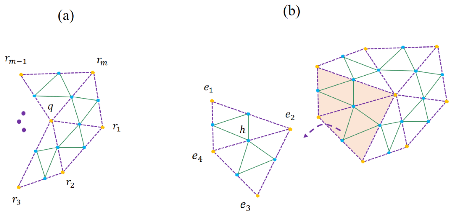
Figure 3 Averaging step of generating the smooth surface by the Loop subdivision scheme. (a) Updating the position of the existing vertices. (b) Updating the position of the new midpoint vertices.

2.1.2 Piecewise smooth subdivision surfaces

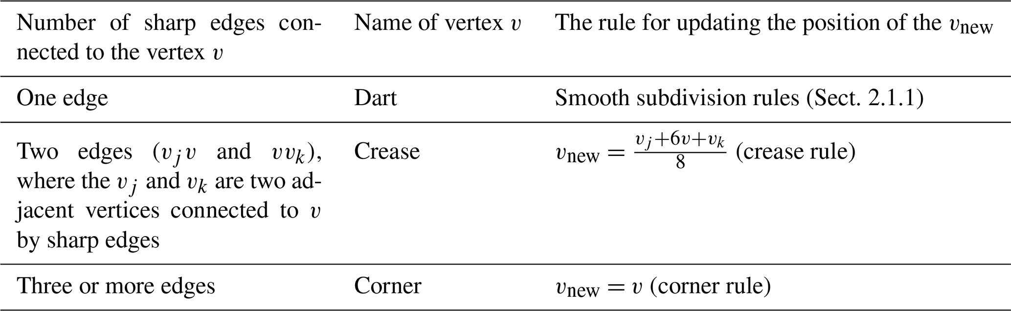
Representation of the objects consisting of sharp features by smooth subdivision algorithms leads to unsatisfactory results. Hoppe et al. (1994) propose to add new rules for the representation of the creases and corners to the Loop subdivision scheme in which the new location of the vertex v depends on the number of connected sharp edges as represented in Table 1 (DeRose et al., 1998).

Table 1 The rules for updating the positions of vertices connected to sharp edges based on piecewise smooth subdivision surfaces (DeRose et al., 1998).

The piecewise subdivision surface method presents an acceptable solution for generating the sharp regions of the model. However, in complex geological modeling, it is vital to model the semi-sharp regions which are not quite sharp.

2.2 Modeling with semi-sharp creases

The creases and corners can be made by considering the crease sharpness values for the edges of the control mesh (Fig. 4). This value can be between zero and one, which indicates zero and infinite sharpness, respectively. Modeling different geometric objects becomes flexible by regulating crease sharpness. As mentioned in Sect. 2.1.2, Hoppe et al. (1994) define the new rules for generating sharp regions during the subdivision procedure. DeRose et al. (1998) generalize the method of Hoppe et al. (1994) for updating the position of the vertices based on semi-sharp subdivision surfaces (Table 2).

Table 2 The rules of the semi-sharp-crease scheme for updating the positions of vertices (DeRose et al., 1998).

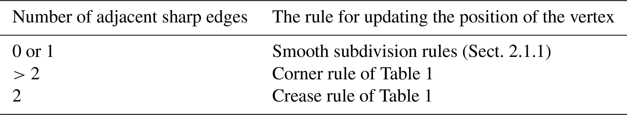
Figure 4a represents the control mesh with eight control points (red vertices). Also, Fig. 4b shows the final smooth mesh after applying the subdivision surfaces algorithm three times when all edges of the control mesh have no crease sharpness values. However, Fig. 4c represents the effect of the resistance of three sharp edges to the smoothing procedure (black edges, with crease sharpness values equal to one).

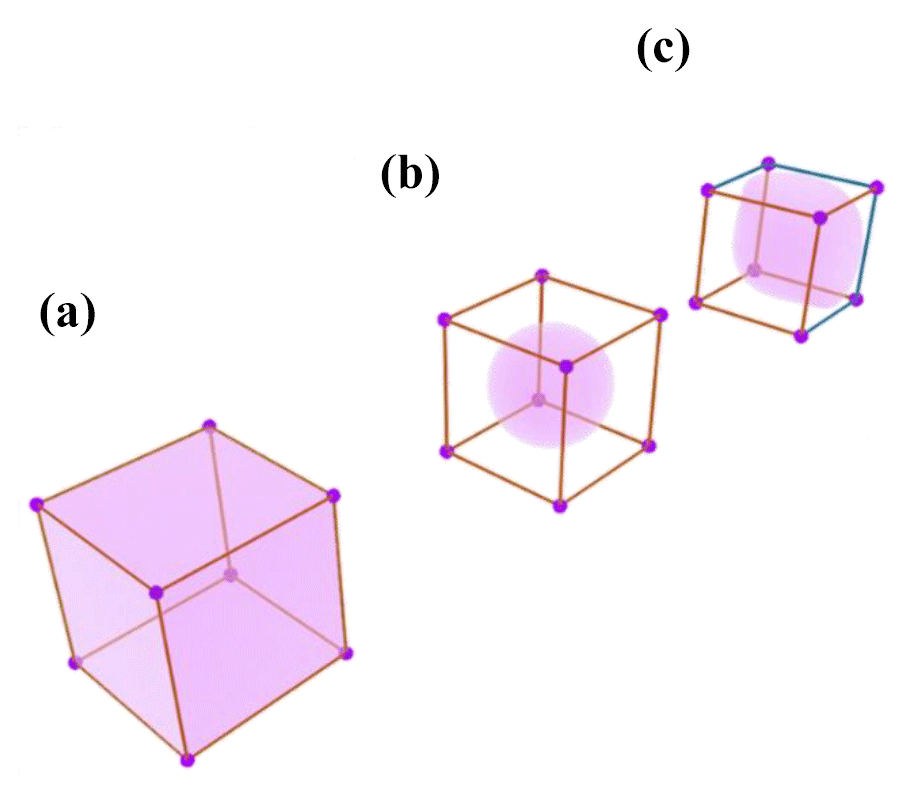
Figure 4 Generating creases on a mesh by applying the subdivision surface algorithm three times (Moulaeifard et al., 2023). (a) Control mesh (b). All edges of the control mesh are smooth edges (red edges). (c) Four edges are crease edges (blue edges), and nine edges are smooth (red edges).

2.3 Supporting non-manifold topology

Non-manifold topologies are extensively observed in complex geological and reservoir modeling. Figure 5 represents the surface intersections as a common example of non-manifold topology in geological modeling where multiple faces are shared by one edge (e.g., the intersection of different faults or intersections between a horizon and a fault).

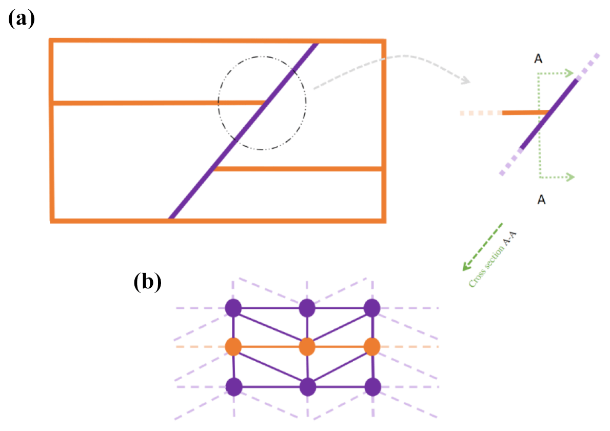
Figure 5 (a) A schematic representation of the intersection between a fault and a layer. (b) Mesh structure of the surface intersection includes the simple singular vertices (brown circles).

The classic subdivision surfaces cannot support non-manifold topology since there is at least one irregular vertex and/or edge. Ying and Zorin (2001) propose the non-manifold subdivision surface algorithm, which supports a wide variety of non-manifold topology problems. A full explanation of this method is beyond the scope of this paper, and in the following, we mention part of their work which is practical in geological modeling. However, Moulaeifard et al. (2023) extensively investigated non-manifold subdivision surfaces for geological and reservoir modeling with multiple examples.

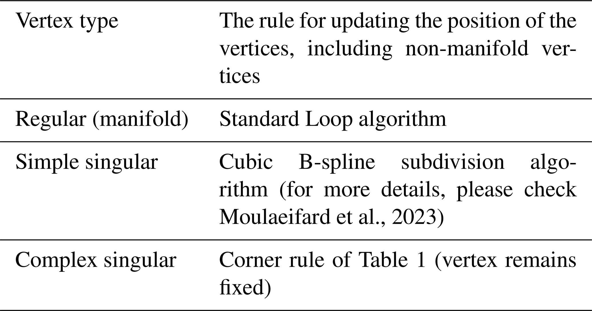
Ying and Zorin (2001) categorize the vertices of the mesh into three types and define the rule for updating the position of vertices (Table 3): (1) regular vertices; (2) simple singular non-manifold vertices that are connected to only two neighborhood vertices by two shared non-manifold edges (Fig. 6); and (3) complex singular non-manifold vertices, which are the other non-manifold vertices. PySubdiv exploits the non-manifold subdivision surfaces for geological modeling.

Figure 6 A representation of the simple singular vertex (v) (Moulaeifard et al., 2023).

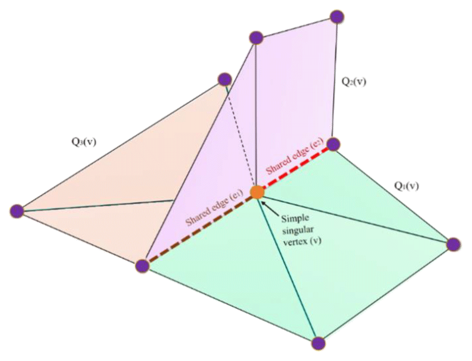
Table 3 The rules for updating the position of the vertices based on the non-manifold subdivision surface algorithm (Ying and Zorin, 2001).

2.4 Automatic reconstruction

The geological model can be constructed by various methods, e.g., marching cube from the implicit model. As mentioned in Sect. 1, the goal of surface reconstruction in this paper is to make the geological model manageable with a few numbers of control points (of the control mesh). In order to reconstruct the input mesh, the control mesh should be estimated first based on the salient features of the input mesh (e.g., the location of minima, maxima and saddle points). Exploiting the salient features of the input mesh leads to preserving the critical features of the input mesh (Ma et al., 2015). Then, the location of the control points and crease sharpness values of the edges are optimized to find the best fit of the reconstructed and input meshes.

It is worth mentioning that applying the subdivision surface algorithm to the watertight control mesh results in a watertight reconstructed mesh. Figure 7 represents the general workflow of the reconstruction process of an anticlinal structure. The input mesh contains two triangulated surfaces, which are generated by GemPy software (De La Varga et al., 2019). In order to obtain the initial control mesh, vertices on the input mesh are extracted (purple spheres) to generate the edges; faces; and, finally, a watertight initial control mesh. The initial control mesh runs through the optimization process to be optimized. The reconstructed mesh is generated by applying the subdivision surface algorithm to the optimized control mesh.

Figure 7 General workflow of subdivision surface fitting with an example of an anticlinal structure.

Also, the following conceptualized approach can be mentioned for the reconstruction process (Fig. 8).

A noisy input mesh ℳ (black curve), e.g., a rough geological interface, is generated from laser scanning or geophysical measurements. A coarse control mesh K (orange curve) is generated based on the features of the input mesh (e.g., minima and maxima), which contains the control points v_i. An unfitted subdivision surface S_K is generated based on the control mesh. On the subdivision surface, s(v_i) indicates the position of vertices v_i after subdivision. Hence, the distances d_i between s(v_i) and the input surface can be calculated by projecting the normal from the input mesh or finding the closest vertices (Marinov and Kobbelt, 2005). Finally, the distance is minimized by repositioning the control points v_i and setting the crease sharpness value to the edges.

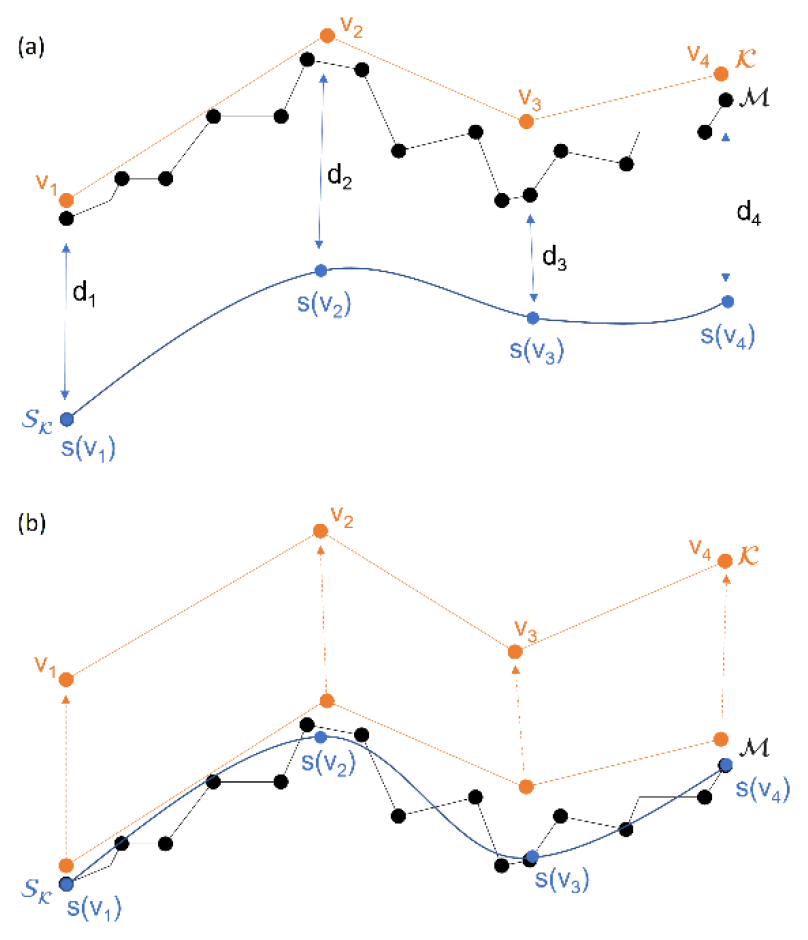
Figure 8 Synthesized and conceptualized approach for surface fitting with subdivision surfaces.

Wu et al. (2017) investigate the automatic reconstruction by solving an optimization problem. In their method, the positions of the control points and the crease sharpness value of each edge repeatedly change until the best fit is achieved. In both manual and automatic methods, the first step is the estimation of the control points (c) with outstanding features of the input geological mesh, e.g., local maxima and minima. PySubdiv proposes some critical points of the input mesh as suitable candidates for the generation of the control mesh. However, it is always possible to arbitrarily select a set of control points. Then PySubdiv used the Delaunay triangulation approach to generate the initial control mesh. The second step is the reconstruction through optimization of the location of control points and crease sharpness value for each edge of the control mesh to find the best fit of the reconstructed mesh to the input mesh.

Assume that the input geological mesh consists of m vertices $q=\left\{q_{\mathrm{1}},q_{\mathrm{2}},q_{\mathrm{3}},\mathrm{\dots }{q}_m\right\}$, the control mesh consists of n vertices $c=\left\{c_{\mathrm{1}},c_{\mathrm{2}},c_{\mathrm{3}},\mathrm{\dots }{c}_n\right\}$, and m edges have crease sharpness values of $h=\left\{h_{\mathrm{1}},h_{\mathrm{2}},h_{\mathrm{3}},\mathrm{\dots }{h}_m\right\}$. The goal is to minimize the vector k, which indicates the difference between q and the projection of q onto the reconstructed (subdivided) mesh. Hoppe et al. (1994) mention that each vertex of the reconstructed mesh can be approximated as an affine combination of control points (c). Therefore the foot point vector of the q on the reconstructed mesh can be approximated as f(h)c, where f(h) is a matrix dependent on h. Therefore, the optimization problem can be represented by

$$\begin{array}{}\text{(4)}& \min ∥k∥,\end{array}$$

subject to $k=q-f\left(h\right)c$. Wu et al. (2017) offer the following augmented Lagrangian function for solving Eq. (4) by using the augmented Lagrangian approach:

$$\begin{array}{}\text{(5)}& \begin{array}{rl}L\left(c,h,k;\mathit{\lambda }\right)& =∥k∥+\langle \mathit{\lambda },\left(k-\left(q-f\left(h\right)c\right)\right)\rangle \\ & +{\displaystyle \frac{b}{\mathrm{2}}}{∥k-(q-f\left(h\right)c)∥}^{\mathrm{2}},\end{array}\end{array}$$

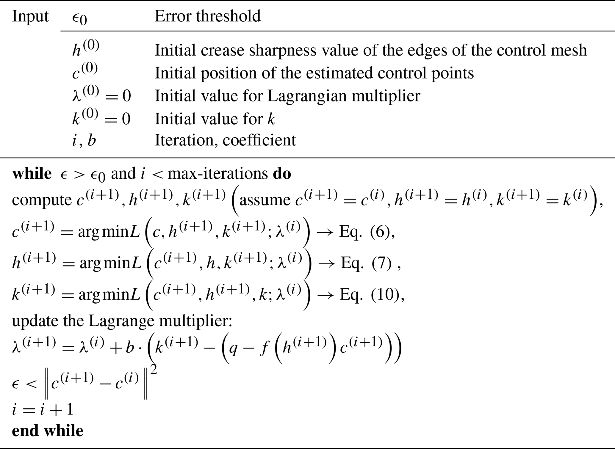
where λ is the Lagrange multiplier, 〈 〉 is the vector dot product operator, and b is a positive number. The following optimization algorithm (Table 4) is used for solving Eq. (5), which includes solving three sub-problems respecting c, h and k at each iteration.

Table 4 Reconstruction by semi-sharp subdivision surfaces based on Wu et al. (2017).

1. Sub-problem with respect to c. The position of the control points c can be calculated in each iteration of optimization by solving Eq. (6), which is a linear problem:

   $$\begin{array}{}\text{(6)}& \underset{c}{min}\left(\langle \mathit{\lambda },(k-(q-f\left(h\right)c\left)\right)\rangle +{\displaystyle \frac{b}{\mathrm{2}}}{∥k-(q-f\left(h\right)c)∥}^{\mathrm{2}}\right).\end{array}$$

2. Sub-problem with respect to h. The crease sharpness values, h, in each iteration can be captured by adapting particle swarm optimization (PSO) (Kennedy and Eberhart, 1995):

   $$\begin{array}{}\text{(7)}& \underset{h}{min}\left(\langle \mathit{\lambda },(k-(q-f\left(h\right)c)\rangle +{\displaystyle \frac{b}{\mathrm{2}}}{∥k-(q-f\left(h\right)c)∥}^{\mathrm{2}}\right).\end{array}$$

3. Sub-problem with respect to the k. In each iteration, k can be calculated by

   $$\begin{array}{}\text{(8)}& \underset{k}{min}\left(∥k∥+\langle \mathit{\lambda },(k-(q-f\left(h\right)c)\rangle +{\displaystyle \frac{b}{\mathrm{2}}}{∥k-(q-f\left(h\right)c)∥}^{\mathrm{2}}\right).\end{array}$$

   Calculating Eq. (8) results in the following:

   $$\begin{array}{}\text{(9)}& \mathrm{1}+\mathit{\lambda }+b\left(k-\left(q-\left(f\left(h\right)c\right)\right)\right)=\mathrm{0}.\end{array}$$

   Finally, k can be computed by

   $$\begin{array}{}\text{(10)}& k=q-f\left(h\right)c-{\displaystyle \frac{(\mathrm{1}+\mathit{\lambda })}{b}}.\end{array}$$

3 Core of PySubdiv

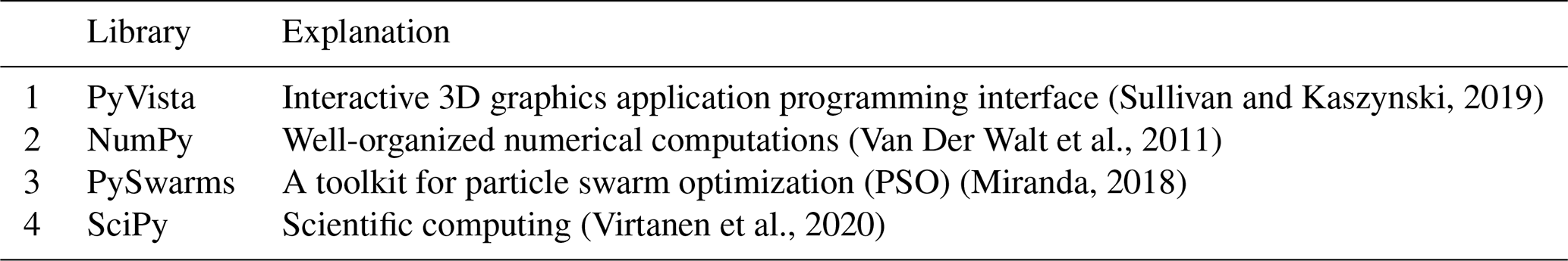
As mentioned in Sect. 2, the core functionality of PySubdiv includes (1) subdivision surface algorithm, (2) modeling with semi-sharp creases, (3) supporting non-manifold topology and (4) automatic reconstruction. PySubdiv is written with an object-oriented approach using the Python programming language (Rossignac and Cardoze, 1999). Also, PySubdiv exploits different varieties of open-source external libraries which are integrated into the core. Table 5 represents the main external libraries implemented in PySubdiv.

Table 5 The main external libraries implemented in PySubdiv.

Step-by-step workflow for the reconstruction of a geological mesh by PySubdiv

(I) Generating the control mesh (semi-automatic)

PySubdiv accepts the structures with the triangle mesh, while the input mesh can be generated by any arbitrary method (e.g., implicit or explicit). Also, the input mesh can be either watertight or non-watertight. If the input mesh is not triangulated, PySubdiv can convert the input mesh to the triangle mesh by using the triangulate function of the PyVista library (Sullivan and Kaszynski, 2019).

The estimation of the position and number of control points is the key stage in reconstruction which leads to the generation of the watertight modeling by providing the control points at surface intersections. PySubdiv offers some candidates to the user based on the features of the input geological structure, e.g., minima, maxima and boundaries. However, it is always possible for the user to select or generate the control points based on the requirements for the interpretation. For example, the geological models generated based on real data may be associated with uncertainties (Wellmann and Caumon, 2018). The user can consider some control points at the suspicious locations regardless of whether the locations are on the boundary or body part of the layer.

In order to show the general workflow of generating a control mesh in PySubdiv, an anticlinal structure model is investigated. Figure 9 represents the graphical user interface (GUI) window of PySubdiv containing the anticline model (two non-watertight surfaces), which is generated by GemPy (De La Varga et al., 2019). It is worth mentioning that watertight or non-watertight meshes can be imported as the input mesh. All of the elements inside the GUI are explained in the Appendix of this paper.

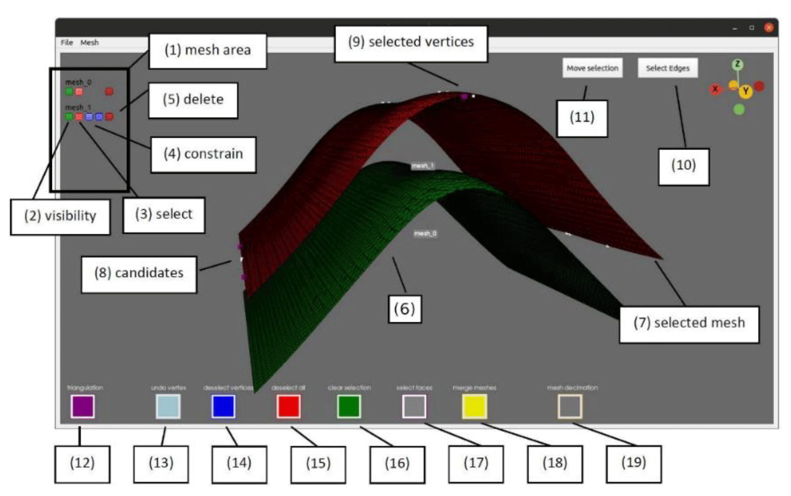
Figure 9 The GUI of PySubdiv allows the user to construct the control mesh for the (geological) model. The important GUI elements are labeled and explained in the following.

First, the top mesh is selected (the color changes from green to red after selection). Then, the control points should be chosen among the vertices of the selected mesh (Fig. 10a). The individual points can be selected by pressing the “P” button on the keyboard while the mouse cursor hovers above them. In this example, the maximal points on the anticline axis have been chosen, as well as an additional point in the center. Three points on the flanks have been sampled to support the control mesh at the turning point. Further important points lie in the corner of the mesh. The next step is to triangulate the selected points. Pressing the triangulation button (12) starts the triangulation. The users are asked if they want to define a polygon used as the “boundary” during the triangulation. If declined, the Delaunay algorithm is executed directly on the automatically detected boundaries. However, unwanted orthogonal faces might appear. It is worth noting that the polygon boundary for the Delaunay algorithm can be defined by the user. Finally, the triangulated control mesh is generated (Fig. 10b). Repeating the mentioned steps for the second input surface yields the second simplified surface for the control mesh.

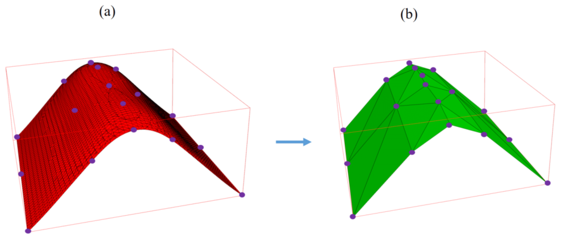
Figure 10 (a) Control points are generated based on the vertices of the input mesh. (b) Triangulated control mesh is constructed based on the control points and the Delaunay triangulation.

In order to create a watertight mesh, four additional sides should be created for the anticline model. Therefore, the boundary vertices of the two simplified surfaces are selected and triangulated. The vertices should be sampled from the simplified surfaces to generate the watertight control mesh (Fig. 11a). At the moment, the four sides must be meshed individually and then merged together. When all four sides are generated, the different meshes can be stitched together by merging. Finally, the sealed control mesh is generated and shown in Fig. 11b.

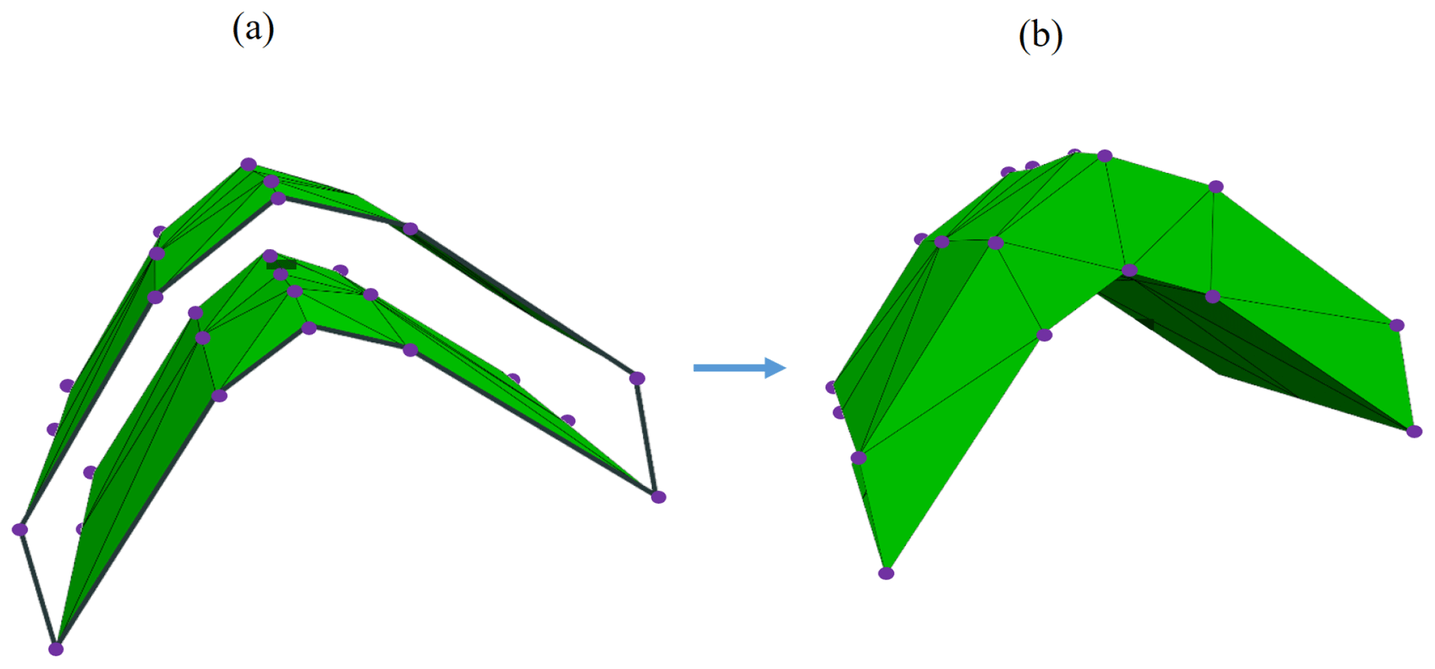
Figure 11 (a) Stitching and merging the different parts of the control mesh to make it watertight. (b) Final watertight control mesh.

(II) set the crease sharpness value to the edges (automatically done by software)

The next step is to assign the crease sharpness value for each edge of the initial control mesh (Fig. 11b). Wu et al. (2017) and Hoppe et al. (1994) suggest a threshold angle (θ₀) as a criterion for tagging the edges of the initial control mesh. The edge is tagged as sharp (i.e., crease sharpness value equal to one) if the angle between the normal of two adjacent faces (θ_e) is more than the threshold angle (θ_e>θ₀). It is worth reminding that this value is just an initial estimation for crease sharpness values.

(III) reconstruction (optimization) of control mesh (automatically done by software)

In the first step of optimization, the generated (initial) control mesh and the original input meshes are imported as the input data for the reconstruction algorithm (Table 4). “MeshOptimizer” class instantiates an object based on the input data, which can start the fitting process with the “optimize” method. It is worth mentioning that the final subdivided (reconstructed) mesh can be exported by applying the subdivision surface algorithm to the optimized control mesh.

4 Case study

As a case study, a part of the Upper Rhine Graben (URG) is reconstructed by PySubdiv. The URG is a long geological structure in the central part of the European Cenozoic Rift System that contains geothermal energy resources. The data set of the URG consists of several different geological units (grid nodes) published by Freymark et al. (2020), which consist of 616 464 individual nodes (Fig. 12). The dimensions of the original model are 292 km in the x direction, 525 km in the y direction and 130 km deep (z direction).

As mentioned in Sect. 3, the input data of PySubdiv should consist of the triangular mesh, which can be generated by any arbitrary method or software. In this case study, PyVista generates the triangular mesh from the individual grid nodes, resulting in 18 different surfaces and 10 volumes.

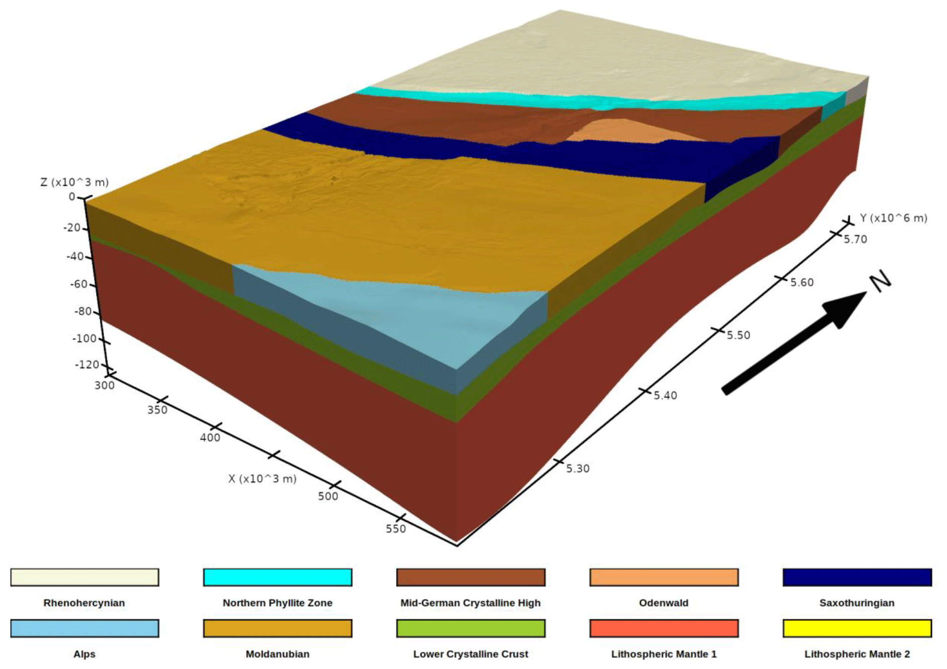
Figure 12 Grid-based representation of part of the URG model, which contains 616 464 individual nodes and 10 different volumes generated based on the data of Freymark et al. (2020).

4.1 Estimation of the control mesh

The initial watertight control mesh is prepared based on the prominent features of the input mesh, such as (a) minimal and maximal points and (b) surface intersections of different layers to ensure that the final mesh is watertight. Figure 13 represents the control mesh consisting of 832 control points distributed over 18 individual surfaces.

Also, the edges of the control mesh, which consist of a threshold angle of 80^∘ (Sect. 3.1), are considered sharp and given the crease sharpness values equal to one. Other edges are considered smooth and assigned crease sharpness values equal to zero. From our experience, exploiting the angle of 80^∘ as the threshold angle in this case study leads to acceptable results. However, this angle can be different depending on the complexity of the model.

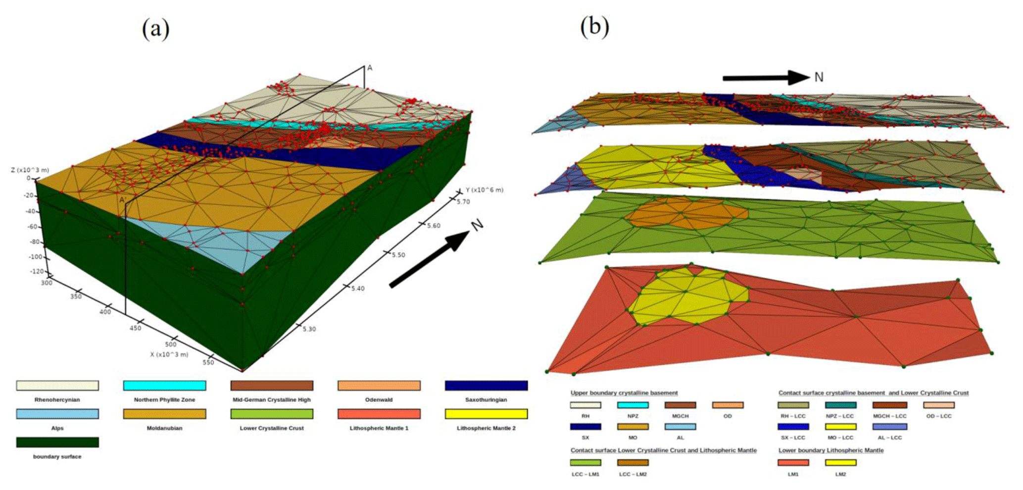
Figure 13 (a) Initial and unfitted control mesh of the URG model. Surfaces are colored concerning the different geological units. The surfaces of the lower crystalline crust and the lithosphere mantle are hidden by the boundary surface. The 832 control points are colored in red. (b) Approximate representation of the 3D side view of the model along the profile AA^′.

4.2 Optimization of the control mesh

The reconstructed mesh is generated after applying two subdivisions to the control mesh (Fig. 14). It consists of roughly 15 000 vertices. In order to evaluate the reconstructed structure, the distance metric between the points of the original and the reconstruction model is computed. Red-colored areas imply high deviations of the subdivided surface from the original model. The mean error for the whole domain is approximately 496±362 m, which is around 0.6 % of the total elevation height. Areas of high error concentrate mainly in regions where two individual geological units are connected and further on the lower boundary of the lithospheric mantle (lower boundaries of Fig. 12). On the lithospheric mantle, the highest errors are up to 5700 m, which is around 4.75 % of the total elevation (approximately 120 km). Most parts of the model consist of small deviations, indicated by the dark-blue color, and the more highly elevated layers are especially well fitted.

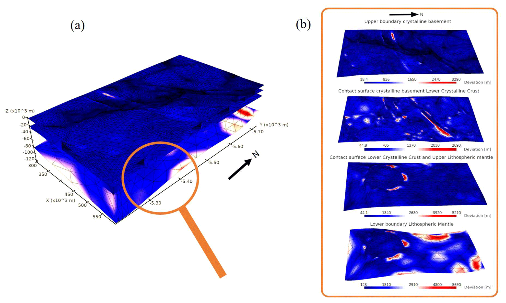
Figure 14 (a) Distance map of the subdivided surfaces compared to the input mesh (Fig. 12). Red areas indicate high deviation from the original input mesh, while blue areas indicate low deviation. (b) Enlarged view of the distance map of the four extracted sub-horizontal layers. Distances are scaled for each layer individually to emphasize the areas of high and low errors independent of the maximal global error.

5 Discussion

The following section discusses the advantages and limitations of PySubdiv in complex geological reconstruction.

5.1 User–PySubdiv interaction

PySubdiv provides a computational framework to generate meshes with limited user interaction. The control points play a key role in estimating, generating and exploiting the reconstruction mesh. The position of the control points can be estimated based on three major criteria: (1) the goal of the user for reconstruction, e.g., uncertainty analysis of the whole or a specific part of the structure; (2) salient features of the input mesh, e.g., maxima, minima and points with high curvature; and (3) surface intersections. Since the goal of the user for reconstruction, e.g. uncertainty analysis of the specific part of the structure, cannot be automatically recognized by the PySubdiv, the user is asked to interact with the software over the GUI to indicate the desired important locations.

However, exploiting the GUI inside the PySubdiv leads to several limitations. As mentioned in Sect. 3, PySubdiv uses PyVista for graphical visualization, which exploits PyQt for the GUI. Some of the PySubdiv users reported the crashes of PyQt with or without any error, especially when using macOS or Windows systems. The current version of PySubdiv suffers from this limitation, which we hope will be solved in future versions.

5.2 Challenges in generating the reconstructed mesh

PySubdiv exploits semi-sharp subdivision surfaces for the reconstruction algorithm which is used by several studies (Lavoué et al., 2007; Wu et al., 2017). However, some studies, e.g., Marinov and Kobbelt (2005), use classic subdivision surfaces for reconstruction. Although using semi-sharp subdivision surfaces would reduce the number of control points, the non-linear role of crease sharpness value in reconstruction optimization cannot be ignored since it is the most time-consuming part of the reconstruction process. As a remedy, the gradient-free method of Powell (1964) of the SciPy library (Virtanen et al., 2020) is implemented instead of PSO in PySubdiv to optimize the non-linear part of the reconstruction. However, it could not significantly reduce the time of this process.

Besides the crease sharpness values, it is worth mentioning that finding suitable locations for the control points based on the salient features of the input mesh is not always easy. For example, assume the geological surface contains two adjacent and approximately flat parts which come close together (Fig. 15). At first glance, this surface has no outstanding features (e.g., min, max, saddle points). However, it is necessary to consider more control points on the boundaries to distinguish the different parts of the surface during the reconstruction process (otherwise, the two different surface parts may be stitched together during reconstruction). This topic is beyond the scope of this paper, and we plan to investigate it in future research.

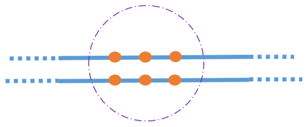
Figure 15 Distinguishing different parts of the surface by adding control points to avoid failure in the reconstruction process.

5.3 External library limitation

From a computational point of view, the major goal of PySubdiv is the calculation of the new location for the vertices of the control mesh based on the subdivision algorithm. Therefore, NumPy (Van Der Walt et al., 2011) and SciPy (Virtanen et al., 2020) libraries play key roles in the core of the software, which can be the source of problems when the input mesh is large, e.g., limited memory.

Although the structure of the PySubdiv is planned to avoid the generation of unnecessary big matrixes, the initial input data can also help to tackle this problem. For example, the suitable number of subdivisions is among the key input data in reconstruction (the number of subdivisions controls the smoothness of the final mesh, which is different from the number of iterations of the optimization process). Applying a small number of subdivisions cannot guarantee the acceptable generation of smooth and semi-sharp parts of a reconstructed mesh. However, applying a large number of subdivisions not only makes no significant differences in the smoothness of the reconstructed mesh but also remarkably increases the unnecessary calculation costs since more subdivisions mean dealing with more vertices.

6 Conclusion

This study illustrated the framework (PySubdiv) to generate suitable control meshes and fitted reconstructed meshes for complex geological structures and reservoir models based on the non-manifold subdivision surface algorithm. The reconstructed mesh is watertight and topologically similar to the input mesh. Also, the control mesh consists of those control points which play a key role in the flexibility and management of the reconstructed mesh. Subdivision surfaces, unlike spline surfaces, support arbitrary topology, which gives more freedom to the user during generation of the control mesh.

Appendix A: Explanation of the elements inside the GUI (Fig. 9) for generation of the control mesh

1. In the mesh area, any mesh resides that is imported or created inside the GUI. The different meshes can be accessed here.

2. This button regulates the visibility of a mesh, helping to keep the viewer clean by disabling unnecessary meshes.

3. This button selects a mesh allowing the user to sample the mesh vertices or edges. Selected meshes are colored red (7). More than one mesh can be selected at a time.

4. The two blue buttons can be toggled to constrain the selection to vertices on the boundary and intersection of two surfaces (left) or to minimal and maximal vertices (right) on the mesh. Constrained points are rendered white (8).

5. The red button deletes the mesh from the viewer.

6. Meshes that are not selected are colored green.

7. The selected mesh appears in red. Only vertices on the selected mesh can be sampled.

8. When a constraint is selected, candidates are shown as white points on the mesh, and only the candidates can be selected.

9. Selected vertices are marked in purple.

10. This button toggles the edge selection and vertex selection. The current selection is cleared when the mode is switched.

11. This button enables one to move the selected points. It also creates a widget that can be moved in space, and the direction is applied to the position of the vertices/edges as a vector.

12. This button triangulates the selected mesh. In PySubdiv, a 2D Delaunay algorithm from PyVista (Sullivan and Kaszynski, 2019) is implemented, which can be bounded by a polygon. Delaunay triangulation is a common method to approximate geological surfaces (Caumon et al., 2009). The polygon can be defined by the user. The order of the polygon is important. If the order is clockwise or counter-clockwise, define the inner boundaries (holes) or the outer boundary.

13. This button removes the last selected vertex from the selection.

14. Switch to deselection mode. Already-selected vertices can be deselected by picking them again.

15. This button deselects all current selected vertices or edges.

16. This button clears the selected vertices, edges and meshes.

17. This button switches to face selection mode. Selected faces can be deleted from the mesh, which is useful when triangulation creates additional faces.

18. This button merges two surface meshes together to form a watertight mesh. In order to form a watertight mesh, vertices on the intersection must be the same on both meshes.

19. This button starts the decimation of a selected mesh. The reduction factor can be set by the user.