the Creative Commons Attribution 4.0 License.
the Creative Commons Attribution 4.0 License.
 | 27 Jun 2023
Leveraging Google's Tensor Processing Units for tsunami-risk mitigation planning in the Pacific Northwest and beyond
Ian Madden
Simone Marras
Jenny Suckale
Tsunami-risk mitigation planning has particular importance for communities like those of the Pacific Northwest, where coastlines are extremely dynamic and a seismically active subduction zone looms large. The challenge does not stop here for risk managers: mitigation options have multiplied since communities have realized the viability and benefits of nature-based solutions. To identify suitable mitigation options for their community, risk managers need the ability to rapidly evaluate several different options through fast and accessible tsunami models, but they may lack high-performance computing infrastructure. The goal of this work is to leverage Google's Tensor Processing Unit (TPU), a high-performance hardware device accessible via the Google Cloud framework, to enable the rapid evaluation of different tsunami-risk mitigation strategies available to all communities. We establish a starting point through a numerical solver of the nonlinear shallow-water equations that uses a fifth-order weighted essentially non-oscillatory method with the Lax–Friedrichs flux splitting and a total variation diminishing third-order Runge–Kutta method for time discretization. We verify numerical solutions through several analytical solutions and benchmarks, reproduce several findings about one particular tsunami-risk mitigation strategy, and model tsunami runup at Crescent City, California whose topography comes from a high-resolution digital elevation model. The direct measurements of the simulation's performance, energy usage, and ease of execution show that our code could be a first step towards a community-based, user-friendly virtual laboratory that can be run by a minimally trained user on the cloud thanks to the ease of use of the Google Cloud platform.
- Article
(5386 KB) - Full-text XML
- BibTeX
- EndNote


The coast of the Pacific Northwest, from Cape Mendocino in California to northern Vancouver Island in Canada, as depicted in Fig. 1, is located on the seismically active Cascadia subduction zone (Heaton and Hartzell, 1987; Petersen et al., 2002). Along the 1200 km long Cascadia subduction zone, there have been no large, shallow subduction earthquakes over the approximately 200 years of modern-data monitoring, but large historic earthquakes have left an unambiguous imprint on the coastal stratigraphy (Clague, 1997). Sudden land level change in tidal marshes and low-lying forests provide testimony to 12 earthquakes over the last 6700 years (Witter et al., 2003), including one megathrust event that ruptured the entirety of the current Cascadia subduction zone in 1700 BCE (Nelson et al., 1995; Wang et al., 2013). The event created a massive tsunami that swept across the entire Pacific Ocean, devastating communities as far away as Japan (Satake et al., 1996; Atwater et al., 2011). Current seismic-hazard models estimate that the probability of another magnitude 9+ earthquake happening within the next 50 years is about 14 % (Petersen et al., 2002).
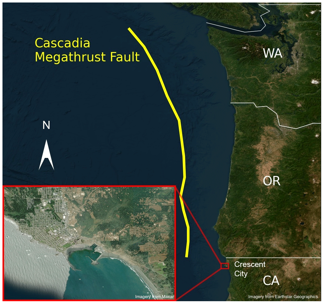
Figure 1Map of the Cascadia subduction zone in the Pacific Northwest of the United States. Relative location of Crescent City with respect to the megathrust fault line, with a more detailed picture of the Crescent City coastline. Esri provided access to the satellite imagery. Crescent City map at high resolution provided by Maxar. Pacific Northwest map provided by Earthstar Geographics.
A magnitude 9+ Cascadia earthquake and tsunami occurring during modern times would devastate many low-lying communities along the Pacific Northwest. A recent assessment suggests that deaths and injuries could exceed tens of thousands and entails economic damages on the order of several billions of dollars for Washington and Oregon State (see, Knudson and Bettinardi, 2013; Gordon, 2012), with potentially severe repercussions for the entire Pacific coast and country as a whole. The tsunami itself would put tens of thousands of people at risk of inundation, and threaten the low-lying coastal communities specifically in the Pacific Northwest with very little warning time for evacuation (Gordon, 2012). But how to confront this risk? Traditionally, the most common approach to reducing tsunami risk is the construction of seawalls, but this hardening of the shoreline comes at a staggering price in terms of the economic construction costs (e.g., 395 km of seawalls in Japan cost USD 12.74 billion) and in terms of long-term negative impact on coastal ecosystems (Peterson and Lowe, 2009; Dugan and Hubbard, 2010; Bulleri and Chapman, 2010) and shoreline stability (Dean and Dalrymple, 2002; Komar, 1998).
A potentially appealing alternative to seawalls are so-called hybrid approaches. Hybrid risk mitigation combines nature-based elements and traditional engineering elements to reduce risk while also providing co-benefits to communities and ecosystems. An example of a hybrid approach to tsunami-risk mitigation is a coastal mitigation park: this is a landscape unit on the shoreline built specifically to protect communities or critical infrastructure and provide vertical evacuation space, in the styles of Fig. 2. Communities across the Pacific Northwest are increasingly considering these nature-based or hybrid options (Freitag et al., 2011), but many important science questions regarding protective benefits and optimal design remain open (Lunghino et al., 2020; Mukherjee et al., 2023). This gap is particularly concerning given that existing models show that a careful design is necessary to avoid potential adverse effects (Lunghino et al., 2020). The design of current mitigation parks, such as the one being built in Constitución, Chile, is not yet underpinned by an in-depth quantification of how different design choices affect risk-reduction benefits, partly because numerical simulations of tsunami impacts are computationally expensive.
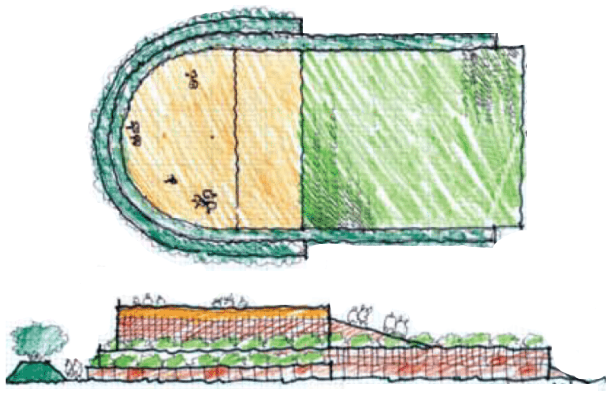
Figure 2Map view (top) and side view (bottom) of a proposed tsunami-mitigation berm as designed by Project Safe Haven. The berm provides vertical evacuation space for the adjacent community and could also lower the onshore energy flux that drives the damage created by tsunami impact. We show this design as one example of a hybrid approach to tsunami-risk mitigation as it combines an engineered hill and ramp with natural vegetation. Sketches are adapted from Freitag et al. (2011).
The goal of this paper is to leverage Google's Tensor Process Units (TPUs) for enabling a fast evaluation of different mitigation park designs and
ultimately advancing evidence-based tsunami-risk mitigation planning rooted in quantitative assessments. TPUs are a new class of hardware accelerators
developed by Google with the primary objective of accelerating machine learning computations. They are accessible via the Google Cloud Platform
(Jouppi et al., 2017) and have recently been used for many different applications in computational physics and numerical analysis
(Wang et al., 2022; Hu et al., 2022; Lu et al., 2020b, a; Belletti et al., 2020). We build upon and extend an existing implementation
(Hu et al., 2022) to simulate the impact of idealized tsunamis on the coastline. Our implementation of the shallow-water equations includes a
nonlinear advective term not considered in (Hu et al., 2022), within the software framework based on Google's TensorFlow necessary to
execute code on the TPU. We discretize the new equations using the weighted essentially non-oscillatory (WENO) method (Liu et al., 1994) and a
third-order Runge–Kutta scheme in time.
Numerical simulations of tsunamis have contributed to our understanding of and ability to mitigate wave impacts for many decades now, starting from the early work by Isozaki and Unoki (1964) for Tokyo Bay, and Ueno (1960) for the Chilean coast. The ability to capture the rupture mechanism that generates the initial condition for tsunami propagation then enabled the reproduction of many historical tsunamis (Aida, 1969, 1974). Since then, many numerical models have been developed to simulate tsunami generation (Borrero et al., 2004; Pelties et al., 2012; López-Venegas et al., 2014; Galvez et al., 2014; Ulrich et al., 2019), propagation (Titov et al., 2005; LeVeque et al., 2011; Chen et al., 2014; Allgeyer and Cummins, 2014; Abdolali and Kirby, 2017; Bonev et al., 2018; Abdolali et al., 2019), and inundation (Lynett, 2007; Park et al., 2013; Leschka and Oumeraci, 2014; Chen et al., 2014; Marsooli and Wu, 2014; Maza et al., 2015; Oishi et al., 2015; Prasetyo et al., 2019; Lunghino et al., 2020) by solving different variations of the shallow-water and Navier–Stokes equations.
The list of existing numerical models is long and was recently reviewed by Marras and Mandli (2021) and Horrillo et al. (2015). Some commonly used ones are FUNWAVE (Kennedy et al., 2000; Shi et al., 2012), pCOULWAVE (Lynett et al., 2002; Kim and Lynett, 2011), Delft3D (Roelvink and Van Banning, 1995), GeoCLAW (Berger et al., 2011), NHWAVE (Ma et al., 2012), Tsunami-HySEA (Macías et al., 2017, 2020b, a), and FVCOM (Chen et al., 2003, 2014). Our work here relies on well-known numerical techniques to solve idealized tsunami problems. Its novelty lies in demonstrating the capability and efficiency of TPUs to solve the nonlinear shallow-water equations to model tsunamis.
We intentionally use a hardware infrastructure that is relatively easy to use and accessible without specific training in high-performance computing. For the TPU infrastructure that we use here, comprehensive tutorials using Google Colab are available at https://cloud.google.com/tpu/docs/colabs (last access: 6 June 2023). The TPU may increasingly become a standard hardware on which physics-based machine-learning algorithms will be built (Rasp et al., 2018; Mao et al., 2020; Wessels et al., 2020; Fauzi and Mizutani, 2020; Liu et al., 2021; Kamiya et al., 2022). Through its relative ease of access and potential for rapid simulation capabilities, cloud computing provides a valuable alternative to higher-performance computing clusters (Behrens et al., 2022; Zhang et al., 2010), particularly for communities with limited access to local clusters. By leveraging these benefits of the Google Cloud TPU, we propose our implementation as one step towards a community-based, user-friendly virtual laboratory that can be run by a minimally trained user on the cloud. The tool, which is freely available on GitHub (tsunamiTPUlab, 2023) under an Apache License, Version 2.0, for collaborative open-source software development, can be modified to include machine learning capabilities and, eventually, extended to coupled models for earthquake generation, inundation, and human interaction.
Numerical approximation
We model tsunami propagation and runup with the 2D nonlinear shallow-water equations in the conservative formulation with a source term in a Cartesian coordinate system. Letting denote position, we define u(x,t) and v(x,t) as the flow velocities in the x and y directions, respectively. We define h(x,t) as the dynamic water height and b(x) as the imposed bathymetry, meaning that the quantity h+b represents the water surface level. We solve for h, hu, and hv in our implementation. We further place a lower bound h≥ϵ in all cells, meaning no properly “dry” cells are present, and handle cells with water depth h=ϵ (the value of ϵ is problem dependent and on the order of centimeters) using the TPU code provided by Hu et al. (2022). This ensures that no flux arrives from those cells with water height ϵ. While this approach has some important drawbacks (Kärnä et al., 2011), it has been used extensively (Bates and Hervouet, 1999; Bunya et al., 2009; Gourgue et al., 2009; Nikolos and Delis, 2009; Marras et al., 2018) and is sufficient to keep the code stable within the scope of this study. This leads to the following system of equations, a set very similar to that suggested by Xing and Shu (2005):
where g = 9.81m s−2 is the acceleration of gravity, and n is the Manning friction coefficient. Note that the left-hand side of our formulation of the shallow-water equations includes the full nonlinear advection terms.
For ease of future notation, we let , and we rewrite the above equations in a vector form, namely,
where F and G are the fluxes in the x and the y directions for the vector u, and S is a source term arising from variations in topography and Manning coefficient.
We implement these shallow-water equations using the finite volume method whereby the half-step flux and height values are determined through a fifth-order WENO scheme (Liu et al., 1994; Jiang and Shu, 1996). We approximate solutions to cell-wise Riemann problems by formulating fluxes using the Lax–Friedrichs method as in LeVeque (2011). We formulate the bed source term as suggested by Xing and Shu (2005) and formulate the friction term explicitly rather than using the implicit process suggested by Xia and Liang (2018). We use a third-order, total variation diminishing Runge–Kutta scheme (Shu, 1988) to step the numerical solution forward in time.
We begin the discretization of the equation in continuous variables t, x, and y, using respective step sizes Δt, Δx, and Δy, which indicate the distance between consecutive integral steps in the discrete indices n, i, and j, respectively. We use the fifth-order WENO scheme in the x and y directions, where two values of each quantity h, hu, and hv are determined at each half-step of x and y. These two values correspond to a positive and negative characteristic, due to the nature of the footprint that is chosen at a given point. In other words, given the conservative form with relevant variable u, ui,j centered on a finite volume cell, we label these outputs of WENO:
From here, we use the Lax–Friedrichs method to approximate flux values that serve as solutions to the Riemann problem; that is, we approximate
where αu is the associated Lax–Friedrichs global maximum characteristic speed. Now, we discretize Eq. (4) explicitly as
Note that in our case we also choose to formulate the source term explicitly and centered at the grid point. Since we use an entirely explicit formulation, we can rewrite Eq. (7) as a time-stepping operator for un+1, namely, . Because the Runge–Kutta scheme uses multiple stages within each time step, we reassign the output of the T operator to be , where (n+1) indicates an intermediate full time step forward. This means a full Runge–Kutta step progresses as follows:
The process outlined by Eq. (8) outputs a final un+1 representing a full-step forward in simulation time.
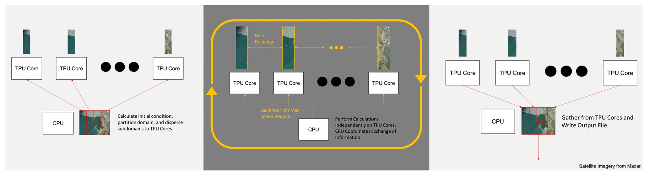
Figure 3Left: initialization of implementation takes advantage of CPU to allocate initial conditions and topography. Center: regular computation period occurring on each subdomain, run independently on TPU cores with some data sharing coordinated by CPU. Right: CPU gather to write results to output files. Esri provided access to the satellite imagery. Crescent City map at high resolution provided by Maxar.
TPU implementation
To leverage the TPU's several cores, we divide the domain into multiple subdomains and independently compute the numerical solution to the governing equations on each core. While a lot of the computation can take place independently, each subdomain remains dependent on the others via their boundaries and the Lax–Friedrichs global maximum in characteristic speed. We determine global maximum characteristic speed by sharing and reducing the Lax–Friedrichs maximum characteristic speed calculated on each core. We transfer subdomain boundary information with further care by using a halo exchange. The data transfer behavior and computation structure is summarized in Fig. 3.
Our implementation is inspired by Hu et al. (2022), who chose halo exchange as an instrument for the TPU to communicate information across subdomain boundaries in their formulation of the shallow-water equations. In the halo exchange process, we transfer slices of the domain from one core to the others immediately adjacent. While the methodology by Hu et al. (2022) only involved the exchange of a single slice from one core to the other, we transfer several slices in order to take full advantage of the high accuracy and larger footprint of the WENO scheme. These halo exchanges are then performed in every stage of the Runge–Kutta scheme, meaning that they occur multiple times in a single time step.
The initial conditions and results are communicated from the remote program, which resides on the CPU, to the TPU workers by means of
tpu.replicate which sends TensorFlow code to each TPU. We refer to Hu et al. (2022) for further details on the TPU
implementation.
We differentiate between model verification and validation in the manner suggested by Carson (2002). Specifically, we check for model and implementation error by quantifying the extent to which numerical solutions compare to correct analytical solutions (Carson, 2002): wet dam break (Sect. 2.1), oscillations in a parabolic bowl (Sect. 2.2), and steady-state flow down a slope with friction (Sect. 2.3). Following this, we validate by checking how well numerical solutions reflect the real system and apply to the context (Carson, 2002). To do this, we compare against an existing numerical benchmark from the Inundation Science and Engineering Cooperative (ISEC, 2004) and results from an investigation of nature-based solutions (Lunghino et al., 2020) in Sect. 2.4, and we consider the propagation of a computed tsunami over the observed topography of Crescent City in Sect. 2.5.
To quantify the accuracy of the solutions, we test our numerical solver against some classical analytical solutions to the shallow-water equations. We assess the model's ability to capture key physical processes relevant to inundation, including steep wave propagation, friction, and topography dependence. We use relative errors in the L∞ and L2 sense as the metric to determine model accuracy. These are approximated in this paper in the following manner:
where hc is the computed solution at the discretized cells, ha is the analytical solution at the corresponding cells, and Ω denotes the computational domain. We omit the cell sizes that often serve as weights in the L2 relative error norm, because all of our cells have the same size. The L2 relative error norm indicates the sum total error in water levels throughout the entire domain, while the L∞ norm indicates the maximal error in a single cell's water level compared to the actual solution.
We refer interested readers to the Appendix B for the corresponding grid convergence analysis under these relative error norms for the first three analytical cases, and we refer readers to Sect. 3.2 for grid convergence analysis of the tsunami modeling in the context of the Inundation and Science Engineering Cooperative (ISEC) benchmark as well as the Crescent City scenario.
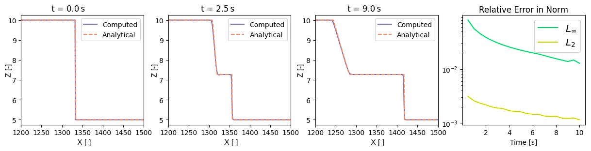
Figure 4On the left, several instances in time of the computed (purple) water heights to wet dam break compared with the analytical (orange, dashed) water heights. The rightmost figure plots the L2 and L∞ relative norms of the error between the analytical and computed solutions.
2.1 Wet dam break
The classical one-dimensional wet dam break scheme (Stoker, 1957) provides us with an opportunity to test the ability of our code to capture shock propagation and advection. In this case, there is no friction (n=0) and the topography is flat (b(x)=0). The boundaries are set at a constant height with zero flux. We impose the following initial conditions:
where hl and hr are the constant water heights on either side of a shock front x0. We compare our numerical solution for water height against the dynamic analytical solution from Delestre et al. (2013):
A qualitative comparison of the computed and analytical solutions for times t = 0, 2.5, and 9 s is shown in the left plots of Fig. 4. The relative error between the analytical and computed solutions in the infinity and 2-norms at a short distance away from the shock front are plotted on the right. We interpret the converging relative error norms to a low magnitude as verification of our implementation to sufficiently capture shock propagation and advection.
2.2 Planar parabolic bowl
The classical one-dimensional planar parabolic bowl, originally suggested by Thacker (1981), is an oscillating solution allowing us to test the source term for topography without friction (n=0). We enforce homogeneous Dirichlet conditions in both flux and water height, at a resolution of 1 m. Once again, we take the test directly from Delestre et al. (2013), resulting in the following description of the base topography:
corresponding with the following initial conditions:
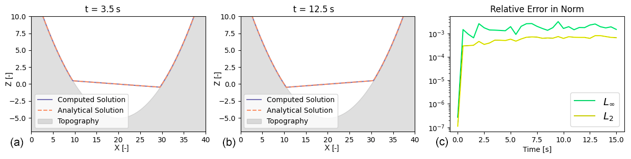
Figure 5On the left (a, b), several instances in time of the computed (purple) water heights to the one-dimensional parabolic bowl compared with the analytical (orange, dashed) water heights. The rightmost figure (c) plots the L2 and L∞ relative norms of the error between the analytical and computed solutions.
This leads to the following dynamic analytical solution for the water height:
where . A qualitative comparison of the parabolic bowl solution at the time instances t = 3.5 and t = 12.5 s can be seen on the left of Fig. 5. The analytical and computed solutions appear to correspond to one another well. For a more quantitative analysis, the relative error norms of the solutions are depicted on the right of Fig. 5. We interpret the converging relative error norms to a low magnitude as verification of our implementation to sufficiently capture the source term of the shallow-water equations induced by topography.
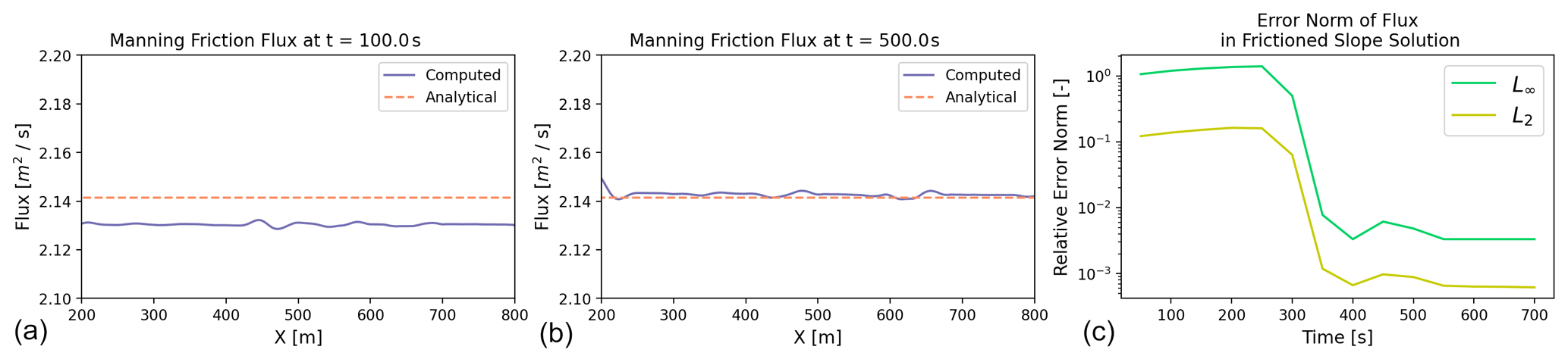
Figure 6On the left (a, b), several instances in time of the computed (purple) fluxes given a water level and a slope, compared to the analytical (orange, dashed) flux. The rightmost figure (c) plots the L2 and L∞ relative norms of the error between the analytical and computed solutions.
2.3 Steady flow down a slope with friction
We do a short test in order to assess the correctness of the discretized friction source term, focusing on a relatively simple flow down a slope with finite friction (n=0.033) as tested by Xia and Liang (2018). The steady-state flow down a slope then becomes
where bx is the slope. In this test, we initialize the problem with a wave height of 0.5 and a slope of , while allowing the flux to start at zero. This specific example and its convergence towards steady state is shown in Fig. 6. The left plots show the flux at t = 100 s and t = 500 s. We see that the flux rises from zero towards the steady-state flux level. On the right plot, the error norm of the steady-state flux takes some time to reach steady state, but reaches a very low level upon reaching time t=500 s. Because we approach the appropriate steady-state solution and achieve a very small error norm, our implementation is verified in capturing a manning friction law.
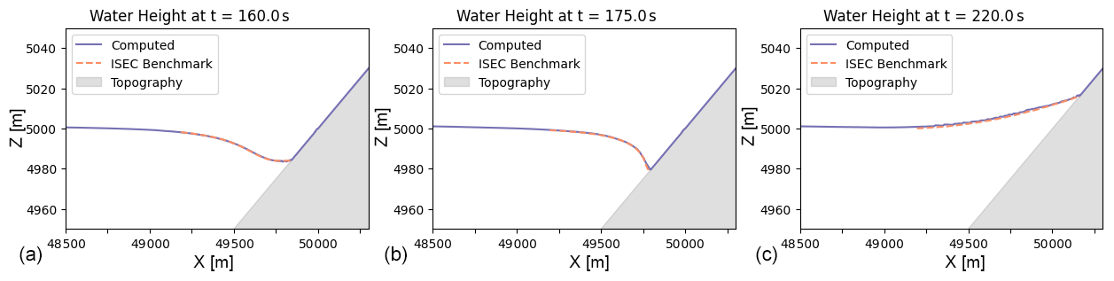
Figure 7Qualitative comparison of the computed solution with resolution 1 m compared to the ISEC benchmark at three different time instances.
2.4 Validation for tsunami simulations
To assess the ability of the code to capture tsunami propagation, we start with a popular numerical benchmark from the ISEC (ISEC, 2004) that represents tsunami runup over an idealized planar beach that provides solutions for tsunami runup at times t = 180, 195, and 220 s. We formulate the initial conditions for water height using Lunghino et al. (2020). The solutions from the benchmark (dashed, orange) are qualitatively compared with the numerical solution produced by our code (solid, purple) in Fig. 7. We take the qualitative agreement as validation of the model's ability to model the runup of a Carrier “N-wave” (Carrier et al., 2003).
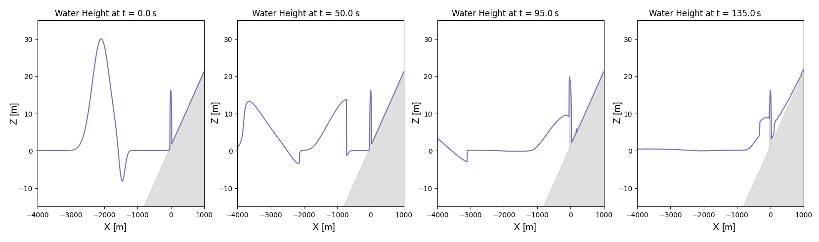
Figure 8Several snapshots in time of the tsunami's propagation over a modeled ellipsoidal hill on a slope. From left to right, the formulation of the initial Carrier N-wave at t=0, followed by the propagation of a wave front towards the hill at t=50, collision of the wave front of the hill at t=95, and the formation of a reflected wave at t=135.
Since we are interested in leveraging TPUs for tsunami-risk mitigation planning, we take a look at the ability of our shallow-water equation code to reproduce a few particular results by Lunghino et al. (2020), who investigated the effects of hills on a tsunami running up a planar beach. The tsunami is initialized as Carrier's N-wave (Carrier et al., 2003):
where , , , , , a1=A, and . While this is the analytically correct form, the flow origin in the code is not the shoreline, so there are some effective shifts and that we need to do. An example of the Carrier wave initial conditions and offshore propagation behavior for A = 15 m and λ = 2000 m is shown in Fig. 8. We apply free slip, no-penetration boundary conditions to the four domain boundaries, which means that the component of the boundary-normal component of the velocity vector is zero, whereas its tangential component is unaltered. The shallow-water equation model presented in this study is able to reproduce the wave reflection provided by a hill, consistent with results from Lunghino et al. (2020). Because this simulation is possible by the implementation, other further analysis can be conducted to understand the mitigative benefit of other nature-based solutions.
2.5 Real-world scenario
Past tsunamis impacting the west coast of the United States have caused more damage around the harbor of Crescent City in California than elsewhere along the Pacific coast (Arcas and Uslu, 2010). For this reason, we chose an area of approximately 105 km2 around Crescent City to demonstrate the code's ability to capture the impact of an idealized tsunami event for a real location at high resolution. To approximate the actual bathymetry and topography, we use a digital elevation model for this area with uniform grid spacing of 4 m provided by NOAA (NOAA National Geophysical Data Center, 2010; Grothe et al., 2011). For the sake of providing a proof of concept, we initialize the tsunami using the same Carrier's waveform defined above but with the following parameters: A = 10 m, λ = 2000 m, m, and m. The chosen parameters lead to maximum inundation patterns similar to that seen in one modeled extreme scenario from Arcas and Uslu (2010). In Fig. 9, we start with an absence of any nearshore wave (including at t = 50 s) and then a development of a tsunami front that is visible to the shoreline by t = 140 s. That front penetrates the harbor by t = 220 s and is soon followed by the inundation of the coastline as well as reflection of wave energy back to the ocean. We also observe that the mountain range on the upper part of the figure clearly provides a significant protective benefit to the land beyond it.
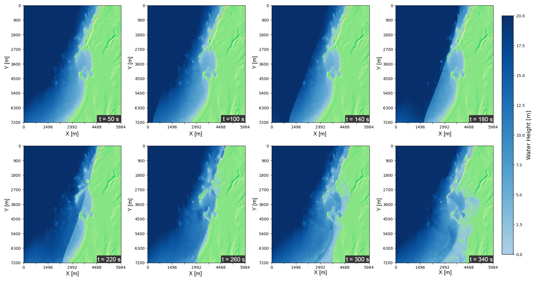
Figure 9Several snapshots of modeled tsunami propagation over terrain and geological features of Crescent City, CA, where any level of blue indicates water cover and where green depicts a stylized map of the topography above surface level. From left to right, then top to bottom, we have a steady state near shore at t = 50 s; followed by the propagation of a wave front at t = 100 and 140 s; contact with Crescent City harbor at t = 180 s; inundation of the harbor and some of the coastline at t = 220 and 260 s; and tsunami reflection and inundation at t = 300 and 340 s.
The protective benefit of the mountain range can be further seen in Fig. 10. This high-water map from a 10 min simulation of runup due to the Carrier N-wave shows the spatial variation of which locations see at least 1 m of inundation under different wave amplitudes. While more work would be necessary to leverage our tsunami software package to connect the inundation by a generated wave to the forcing generated by earthquakes, a risk manager can see how higher-magnitude tsunamis may disproportionately affect certain locations over others.
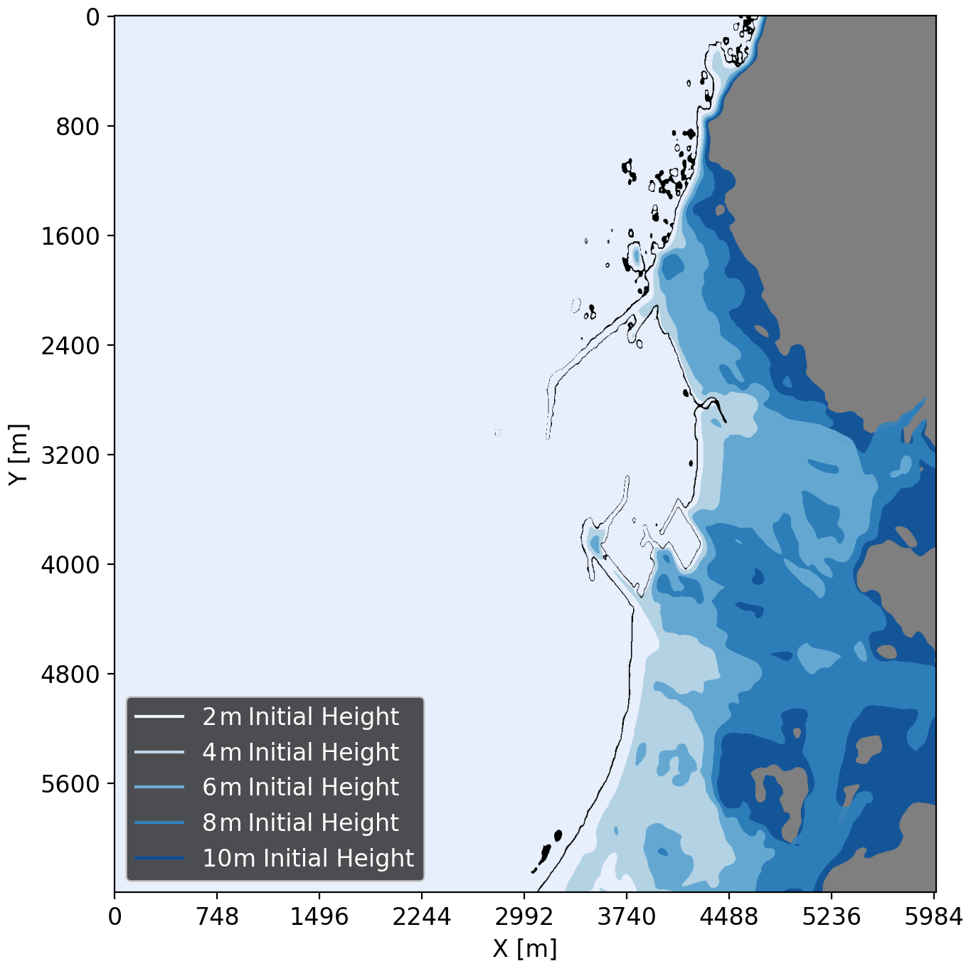
Figure 10The 1 m inundation high-water map for Crescent City, CA, under different amplitude Carrier N-waves initialized 1 km offshore (10 min of simulated time). Darker shades of blue indicate the extent reached by higher-amplitude N-waves.
3.1 Number of TPU cores
As noted in the Introduction, in communities where users may not have access to high-performance computing facilities, the cloud TPU platform provides a particularly valuable resource where users can perform large-scale computations rapidly. To quantify the potential speedup enabled by TPUs with increasing numbers of cores, we observe the average wall-clock time taken in computation for each time step with the exclusion of the first time step. This first time step includes several preprocessing functions, such as reading DEM files into TPU memory, setting up initial conditions, and initializing the TensorFlow workflow. Similarly, we calculate runtime based on the amount of time spent in computation with the exception of this first step, with time which is variable from run to run. As shown in Table 1, the problem size posed by the realistic scenario is sufficient to see rapid improvements in runtime based on the number of cores. We note that our analysis may vary user to user, depending on the TPU version that they are allocated and the number of cores available to them. Our simulations were all conducted with a TPUv2, and we extend our analysis only up to eight TPU cores because, at the time of writing, Google Colab only provides eight cores for free in our region.
Table 1Average TPU runtime per time step (in milliseconds) with varying numbers of TPUv2 cores. The Crescent City configuration at an 8 m resolution is used, with time steps of Δt = 0.02 s for a total of 400 simulated seconds. The domain is a grid of approximately 901 by 1992 elements; TPU cores find solutions to subdomains divided in the y direction as suggested by Hu et al. (2022) and graphically depicted in Fig. 3.
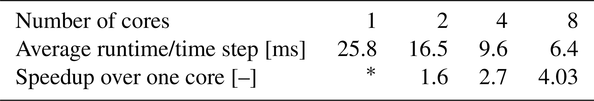
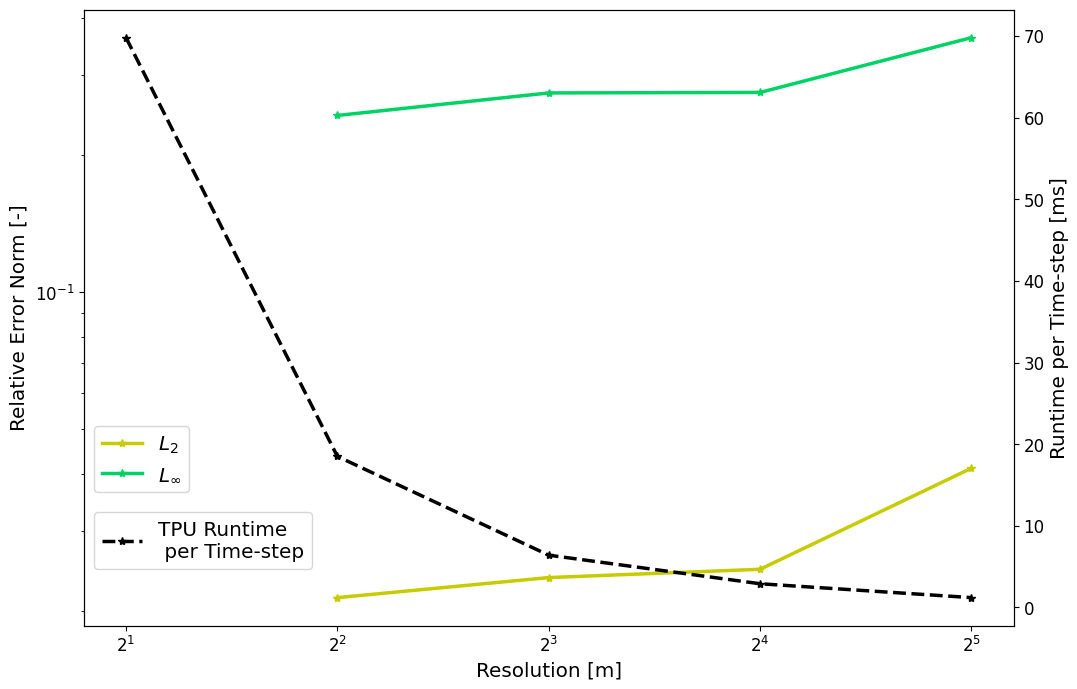
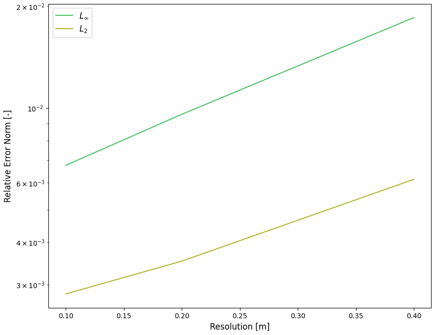
Figure 11Average TPU runtimes per time step (black) and relative L2 (gold) and L∞ (green) norms under varying resolutions for computing the tsunami propagation over the Crescent City DEM.
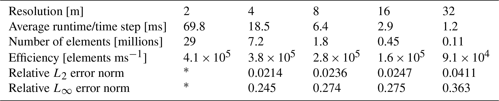
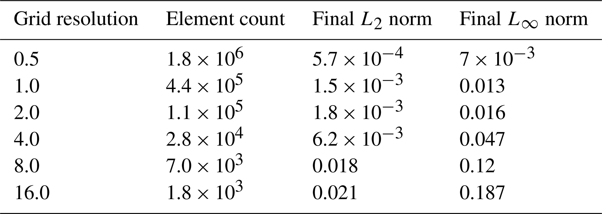
Table 2Approximate TPU runtimes (in seconds) for a 400 s simulation with varying resolutions of the Crescent City configuration using a time step of Δt = 0.02 s. We compute L error norms against the 2 m resolution for correctness at times t = 100, 200, 300, and 400 s in the coastal region. All simulations ran on a single TPUv2 with eight cores.
3.2 Geophysical problem resolution
Simulating tsunami runup typically requires large domains and sufficiently high resolution to accurately capture tsunami propagation and inundation over complex topography. Therefore, we continue analyzing our Crescent City scenario for both convergence and the average runtime spent for each time step under varying degrees of resolution, shown in Fig. 11 and with numerical results given in Table 2. As is expected, relative error norms fall as we reach higher resolutions and lower cell sizes, which in turn corresponds to increasing runtime spent for each time step. To expand upon the scaling of runtime, we calculate an accessory “efficiency” metric to more specifically understand how runtime scales with the number of elements, calculated by dividing the total number of elements over the average runtime per time step. Higher values for this efficiency metric would be associated with a greater number of computations for grid elements being completed per unit time. We see that this efficiency is maximized for high numbers of elements as expected while the TPU reaches capacity.
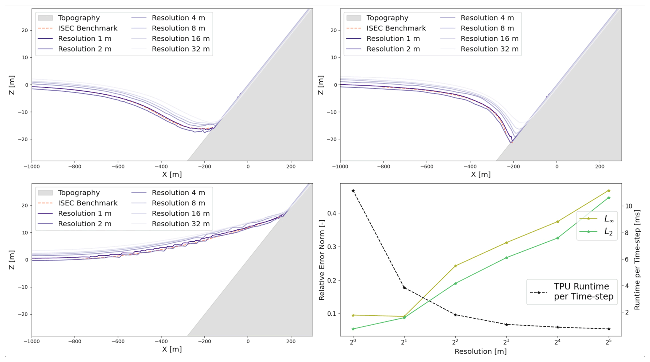
Figure 12(a) ISEC benchmark comparison at 160 s. (b) ISEC benchmark comparison at 175 s. (c) ISEC benchmark comparison at 220 s. (d) TPU runtime for each time step (black) and corresponding relative L2 (green) and L∞ (gold) error norms for varying simulation resolutions.
Table 3Average TPU runtimes per time step (in ms) under varying resolutions for the ISEC tsunami benchmark using a time step of Δt = 5 × 10⁻³ s, along with corresponding L norms calculated with respect to all three times when the ISEC benchmark was available. All simulations ran on a single TPUv2 with eight cores.
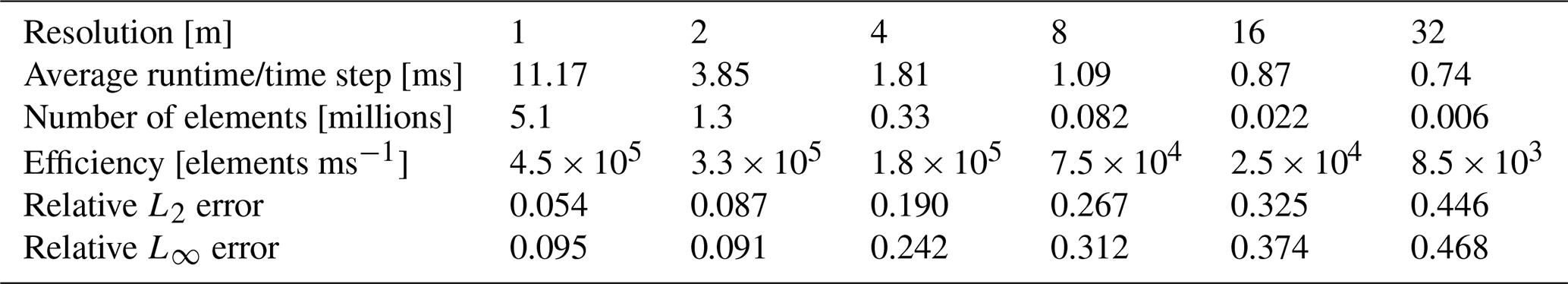
We perform the same analysis under varying degrees of resolution using the benchmark from the Inundation Science and Engineering Cooperative (ISEC, 2004) that we previously validated against in Sect. 2.4. We show a qualitative comparison of the tsunami propagation under different resolutions are graphically depicted in Fig. 12 in the top two and bottom left figures. In the bottom right plot of Fig. 12, we see the expected fall in runtime based on coarser resolution (black), and a rise in relative error, an error representing the accumulation of all three time instances for which the ISEC benchmark is defined. We provide an overview of the corresponding values and efficiency metrics in Table 3. Since the total number of elements is smaller for the ISEC benchmark as compared to the Crescent City scenario, we are able to see even lower efficiency as the TPU is even further away from reaching full capacity.
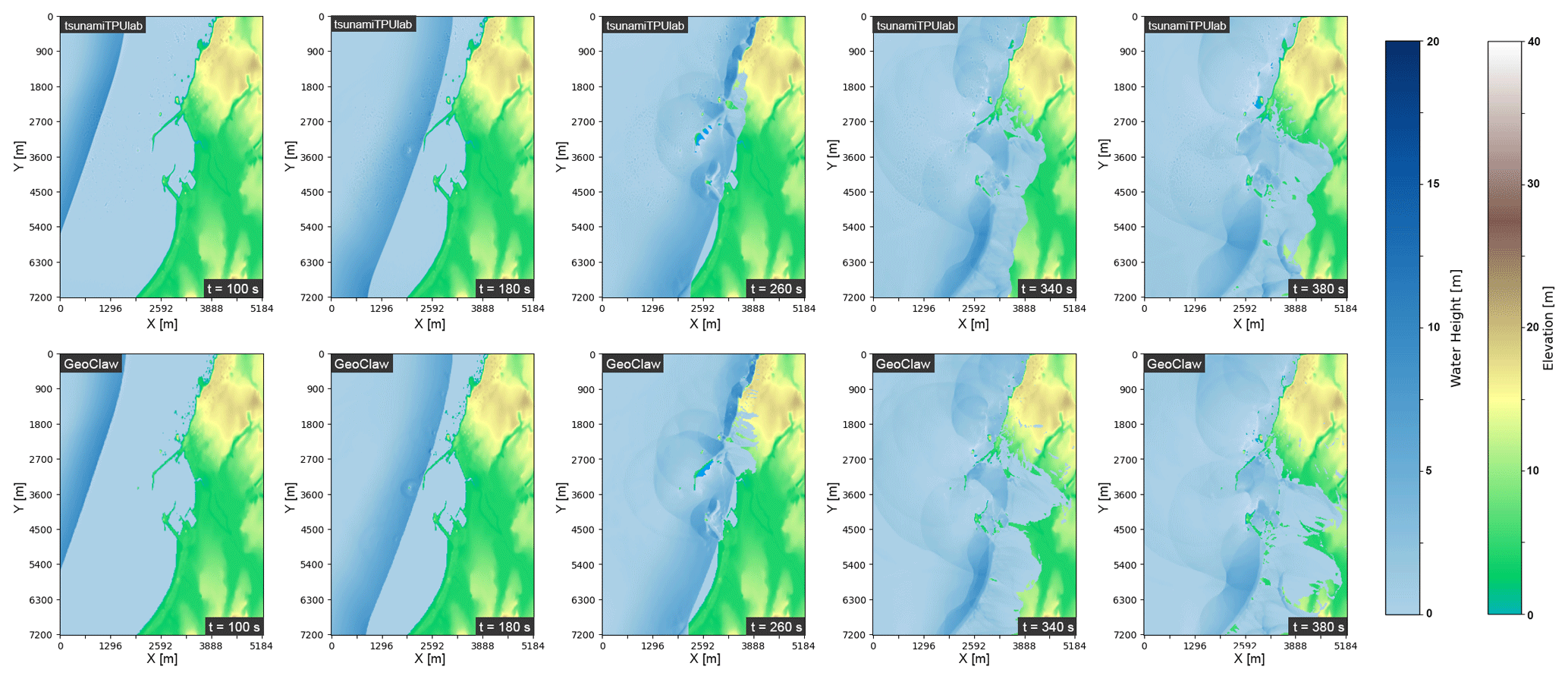
Figure 13TPU solution (top row) at several time instances compared to the GeoClaw solution (bottom row). The arrival of the tsunami front (t = 100, 180 s), the inundation of the harbor (t = 260 s), and coastal inundation and reflection are depicted and relatively comparable.
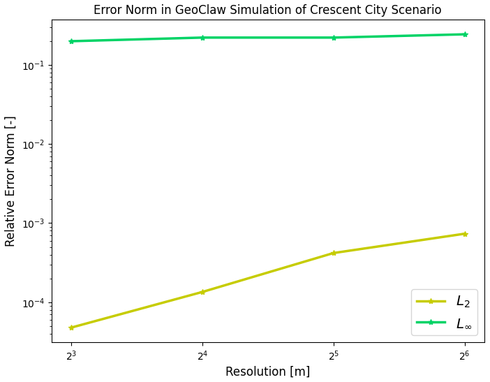
Figure 14GeoClaw relative error norms for a 100 s simulation for our Crescent City scenario under varying resolutions. The 4 m resolution is used as the benchmark.
3.3 Comparison with GeoClaw
For comparison purposes, we run GeoClaw (Clawpack Development Team, 2020; Mandli et al., 2016; Berger et al., 2011) using four CPU threads that were allocated for free via Google Colab. Our GeoClaw simulation uses the same DEM file and is computed at an 8 m resolution without mesh refinement. We use an adaptive time step bounded by the Courant–Friedrichs–Lewy condition, and we determine the spatial fluxes using a second-order, rate-limited Lax–Wendroff scheme. In Fig. 14, we see lower relative error norms as we approach higher resolution in our simulation of our Crescent City scenario. The GeoClaw numerical solution can be compared to our TPU numerical solution in Fig. 13, where the top row includes several instances in time of the TPU numerical solution, and the bottom row depicts the GeoClaw numerical solution at the same instances in time. Although some differences can be seen in inundation by t = 380 s in the rightmost plots, the solutions do generally appear similar over time, lending credibility to the validity of the numerical solution presented in this paper. One particular advantage of our TPU-based code lies in its comparatively rapid simulation. While our TPU-based code completes a 400 s simulation in approximately 2 min of wall-clock time, the adaptive-time-stepping GeoClaw implementation on the CPU takes approximately 275 min. The TPU sees even more significant speedup when we enforce a fixed time step equal to that of the TPU implementation; that GeoClaw simulation would take over 1300 min.
3.4 Energy utilization
Estimates of energy efficiency of computing operations are becoming increasingly popular, especially in response to progressing climate change (Fuhrer et al., 2018; Fourestey et al., 2014). To get a rough approximation of the comparative efficiency of a Google Cloud TPU over a CPU, we ran the Crescent City tsunami propagation problem at 8 m resolution using GeoClaw on a Google Cloud CPU node and our code on a Google Cloud TPU node. We do not have the information nor access to the physical devices needed to conduct rigorous energy profiles to calculate efficiency as is done by others (e.g., Ge et al., 2010), so we deliver an order-of-magnitude estimate based on the thermal design power of the devices that we are allocated via Google Colab. We only compared resources that are freely available through Colab in order to compare the efficiencies of computing resources that may be accessible to all users.
Based on Table 2, each time step takes an average of about 6.4 × 10⁻³ s on the TPUv2 that we were allocated by Google Colab, corresponding to about 0.32 s per simulated second under our current time-stepping regime. The TPUv2 we were assigned contains four chips with a thermal design power of 280 W per chip (Jouppi et al., 2021), meaning that each simulated second then has an energy cost of approximately 0.1 Wh, leading to an approximately 40 Wh energy cost for a 400 simulated-second simulation. At a price of 21 cents kWh−1 in the USA at the time of writing this article, this simulation has a monetary cost of 0.84 cents.
When we ran GeoClaw for our CPU comparison on energy utilization, we enforced a fixed time step on the GeoClaw package of equal size to that of our TPU (i.e., Δt = 0.02 s) rather than leveraging GeoClaw's adaptive time stepping to have a fair comparison in terms of the approximate number of operations. While the specific processor we were allocated for this CPU comparison is not immediately clear, we deduced from the model name, CPU family, and model number that we were allocated the Intel Xeon E5-2650 v4 with a base frequency of 2.2 GHz and a thermal design power of 105 W for 12 cores and 24 threads (Intel, 2016). Of this, we were allocated 2 cores/4 threads, and we took full advantage of all threads for our GeoClaw run. Each time step took approximately 4.2 s, corresponding to about 205 runtime seconds per simulated second. If we assume ideal conditions leading to perfectly proportional scaling of computational speed in increasing cores, we would expect that each simulated second would take approximately 34.2 s when the Intel Xeon E5-2650 v4 was used to full capacity. This means that each simulated second would have an associated energy cost on the order of 1.0 Wh. A 400 modeled-second simulation would imply a total cost of approximately 400 Wh of energy or a monetary cost of 8.4 cents. With the corresponding TPU energy calculation in mind, our conservative estimate suggests that a CPU simulation has approximately 10 times the energy cost of running an equivalent TPU simulation under the same time-stepping conditions.
While these two simulations accomplish the same thing, they have vastly different associated performances. At times, rapid computation and simulations are necessary in the context of risk analysis, and the associated energy costs of such a performant computation is worth estimating. To address this, we push our energy estimate a touch further, providing another order-of-magnitude estimate of what a CPU simulation conducted at TPU performance would be. We extrapolate our previous assumptions further, assuming proportional scaling of computational speed with increasing CPUs and that the thermal design power applies to each CPU within a system independently. Because a simulated second of a full-capacity Intel Xeon E5-2650 v4 CPU takes approximately 34.2 s compared to the TPUv2's 0.32 s, over 100 CPUs at full capacity would be needed for similar rapidity in simulation. Following similar logic as done in the previous paragraph, a CPU simulation of equivalent performance would have approximately 1000 times the energy cost of running a TPU simulation when ran under the same time-stepping conditions.
Sustainable tsunami-risk mitigation in the Pacific Northwest is a challenging task. Some challenges come from beneath, because previous large subduction zone earthquakes at Cascadia led to 0.5–1 m of co-seismic subsidence and the sudden sinking of land during an earthquake (Wang et al., 2013). Strong shaking can also lead to liquefaction (Atwater, 1992; Takada and Atwater, 2004). Other challenges come from the ocean, where sea-level rise (Church and White, 2006; Bindoff et al., 2007) and intensifying winter storms (Graham and Diaz, 2001) have increased wave heights (Ruggiero et al., 2010; Ruggiero, 2013) and accelerated coastal erosion (Ruggiero, 2008). A recent USGS report documented rapid shoreline changes at an average rate of almost 1 m yr−1 across 9087 individual transects (Ruggiero et al., 2013), suggesting the possibility that the shoreline might change significantly during the century-long return period of large earthquakes in Cascadia (Witter et al., 2003).
The picture that emerges is that of a highly dynamic coastline – maybe too dynamic for an entirely static approach. Nature is not only continuing to shape the coastline, but it is also a fundamental component of the region's cultural heritage, identity, and local economy. So, it is maybe not surprising that the Pacific Northwest is a thought-leader when it comes to designing hybrid approaches to sustainable climate adaptation through the Green Shores program (Dalton et al., 2013) and to vertical tsunami evacuation through Project Safe Haven (Freitag et al., 2011).
Project Safe Haven is a grass-roots approach to reducing tsunami risk mostly by providing accessible vertical-evacuation options for communities. Many proposed designs entail reinforced berm like the one shown in Fig. 2, intended to dissipate wave energy and provide vertical evacuation space during tsunami inundation. To build confidence in such a solution and its mitigation effects, risk managers must be able to quickly and precisely forecast a tsunami inundation, preferably via a publicly available, centralized modeling infrastructure.
This paper aims to be a first step towards a community-based infrastructure that will allow local authorities around the world to readily execute tsunami simulations for risk mitigation planning. We aim to provide a proof of concept rather than a complete implementation. As such, we used a very similar base framework used by Hu et al. (2022) of halo exchange in combination with a WENO (Liu et al., 1994; Jiang and Shu, 1996) and Runge–Kutta scheme (Shu, 1988). We choose easily implementable higher-order schemes to maintain high accuracy, necessary for simulating tsunami inundation over the complex topographies that risk managers often deal with in the real world, despite the fact that the large stencils within the current implementation may not be optimal for TPU performance. Future work could consider a convolution-based implementation of the quadrature of the shallow-water equations to test for maximum performance utilization of the TPUs.
Because our code is specifically an implementation of the shallow-water equations, it is currently unable to model tsunami initiation or any fluid structure interactions that may be desired to accompany analysis of nature-based solutions. Instead, it requires an initial condition for wave heights and fluxes, meaning a full tsunami simulation would require coupling the results of a tsunami initiation model as an input. While our implementation is relatively limited in scope, the model is able to provide a starting point for a more complete software package for communities as they evaluate nature-based options for tsunami mitigation.
We argue that cloud TPUs are preferable to large, heavily parallel simulations on CPUs or GPUs for risk managers across all communities, because the TPU-based simulations we show here do not require access to the large computing clusters hosted by laboratories and universities. These clusters require huge amounts of power to run and are usually only made available to scientists and engineers by means of competitive grants for computing time or by use of the cloud offered by private companies. However, an expert user knowledge of these systems from a scientific computing perspective is necessary to design, run, and interpret model results, and the compute infrastructure itself may not be available to early-warning centers in many parts of the world. In contrast, our code is available on GitHub and fully implemented in Python; it can be executed through a web browser and visualized through a simple notebook file using Google Colab without the knowledge otherwise required to run large parallel codes on high-performance computing systems. By taking advantage of Google Cloud Platform, we also ensure that a user's power demand is met entirely with renewable energy (Google, 2022). Performance can be enhanced with some knowledge about TPU architectures, but community risk managers do not need this knowledge to run high-quality tsunami simulations rapidly for real, physical domains with associated DEMs.
Finally, though not our focus here, we note our approach may also contribute to early tsunami warning. Once triggered, tsunamis move fast; this fact makes it necessary to model and assess their potential for damage ahead of time once they have been detected offshore. For a sufficiently fast early warning and prompt evacuation, the tsunami modeling infrastructure has an important time constraint (Giles et al., 2021) to be considered, and faster than real time (FTRT) simulations are necessary (Behrens et al., 2021; Løvholt et al., 2019). To make FTRT simulations a reality, tsunami models are being rewritten or adapted to run on graphical processing units (GPUs) (Løvholt et al., 2019; Behrens and Dias, 2015; Satria et al., 2012). A TPU-based implementation as proposed here might be another meaningful step in that direction.
We present a first step towards an accessible software package that leverages the powers of cloud-based TPU computing for improving the capabilities of risk managers and communities to mitigate the destructive onshore impacts of tsunamis. We verify and validate our current implementation to ensure that it is capable of simulating inundation from a Carrier N-wave over real topography. These simulations are comparable to that ran by the popular open-source solver GeoClaw (Clawpack Development Team, 2020; Berger et al., 2011) but can be run at higher speeds through Google Colab and requires less expertise in scientific computing. As a result, high-quality tsunami simulations are available to remote communities for rapidly evaluating different risk-mitigation options including but not limited to nature-based solutions. Future efforts can then be dedicated to better meeting the needs of risk managers with a platform available through the cloud, be that in coupling our shallow-water equations package to earthquake–tsunami generation models or experimenting with different numerical implementations to enable even more rapid simulation of these equations.
Due to the restrictions of the cloud TPU using Google Cloud Storage, a user must leverage Google's buckets to run the notebooks. At the time of
writing this article, eight TPU cores are readily available in North America on Google Colab for free, but Google Cloud Storage buckets are a paid
subscription service (see https://cloud.google.com/tpu/docs/regions-zones, last access: 6 June 2023, for information about
specific regions). With a computing project setup on Google Cloud and a corresponding bucket with open permissions (with steps specified in
https://cloud.google.com/storage/docs/creating-buckets, last access: 6 June 2023), users can quickly run any of the example
notebooks or design their own simulation. Any of the example notebooks available on GitHub (with the exclusion of tpu_tsunami.ipynb, which
contains the full implementation with all of the different scenarios; and Create_Scenarios.ipynb, which can aid users in generating a custom
DEM file) can be quickly ran by going through the notebook after a few setup steps.
-
Download the TPU-Tsunami Repository from https://github.com/smarras79/tsunamiTPUlab/releases/tag/v1.0.0 (last access: 6 June 2023) to your local machine. Create a project on Google Cloud Platform and associate a publicly available bucket with the project.
-
Modify the
user_constants.pyfile to specify thePROJECT_IDandBUCKETwith the specifics of your Google Cloud project. If you wish to change some simulation constants, modify the beginning of thetpu_simulation_utilities.pyfile. -
Navigate to https://colab.research.google.com/ (last access: 6 June 2023) and open the example notebook (or your own notebook) from the TPU-Tsunami Repository using Colab's “open from GitHub” tool.
-
Navigate to Runtime > Change runtime type, and verify that the TPU option is chosen as the hardware accelerator.
-
Upload your
user_constants.pyandtpu_simulation_utilities.pyfiles to your notebook session using the drag-and-drop feature under “Files”. Upload any corresponding DEM files to the session as well. -
Specify a function corresponding to an initial condition for your DEM file (or use one example initial condition).
-
Set initial conditions and boundary conditions as clarified in the bottom of any example notebook run. Set last simulation parameters defining numerical resolution (
resolution), time step size (dt), output file times, TPU core configuration (currently only capable of variation ofcy), and DEM file name on bucket (dem_bucket_filename). -
Run the simulation.
-
Analyze results.
In addition to the convergence analysis for the ISEC benchmark posed in Sect. 3.2, we have included some additional results constituting a convergence analysis for two of the other analytical scenarios that are particularly relevant for establishing an appropriate grid resolution.
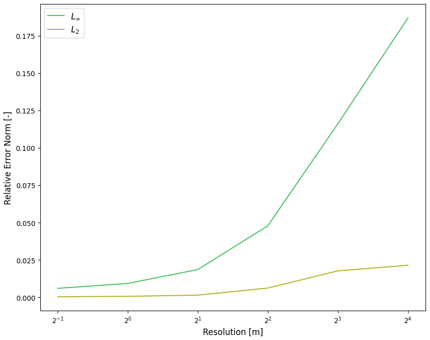
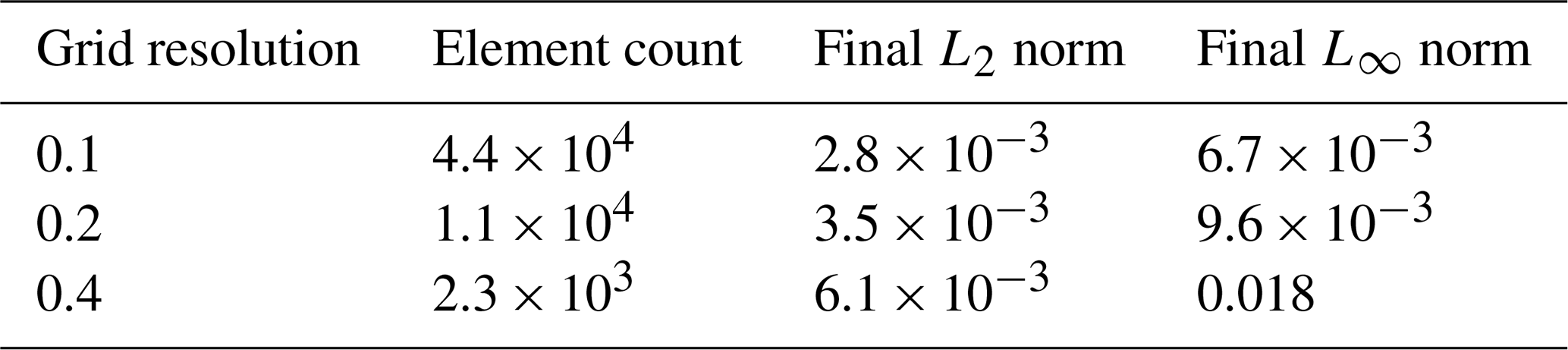
Figure B1Final relative error norms calculated at 10 s into the wet dam break problem under varying resolutions.
Table B1Grid convergence analysis for wet dam break, with values.
In Fig. B1, we can see how the wet dam break case converges with higher resolution. This is more concretely specified in Table B1 with specific values. In Fig. B2, we can see improvements in the grid convergence for the planar parabolic bowl problem from Sect. 2.2. We begin to see error convergence at high enough resolution.
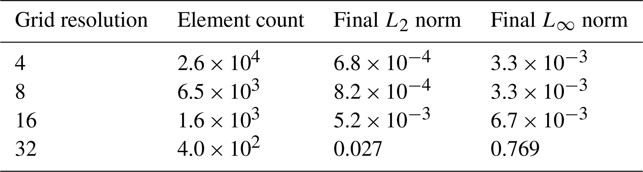
Finally, in Fig. B3, we can see how the wet dam break case converges with higher resolution. This is more concretely specified in Table B3 with specific values. In Fig. B3, we can see improvements in the grid convergence for the slope with manning friction problem from Sect. 2.3.
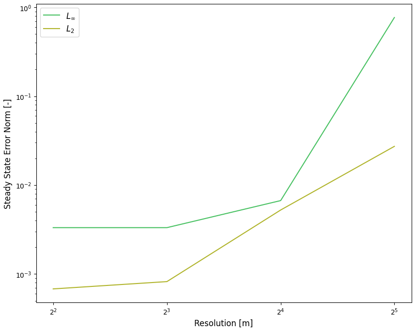
Figure B3Grid convergence analysis using flux as the error metric for slope with Manning friction.
Table B3Grid convergence analysis using flux as the error metric for slope with Manning friction.
Our work is available as a GitHub release at https://github.com/smarras79/tsunamiTPUlab/releases/tag/v1.0.0 (last access: 12 June 2023) or on archive at https://doi.org/10.5281/zenodo.7574655 (Madden et al., 2023).
IM: Methodology, Software, Analysis, and Writing. SM, PI: Conceptualization, Methodology, Writing, and Supervision. JS: Conceptualization, Methodology, Writing, and Supervision.
At least one of the (co-)authors is a member of the editorial board of Geoscientific Model Development. The peer-review process was guided by an independent editor, and the authors also have no other competing interests to declare.
Publisher's note: Copernicus Publications remains neutral with regard to jurisdictional claims in published maps and institutional affiliations.
This work was supported by the National Science Foundation's Graduate Research Fellowships Program (GRFP) awarded to Ian Madden.
This research has been supported by the National Science Foundation’s Graduate Research Fellowships Program (GRFP) awarded to Ian Madden (grant no. DGE-2146755).
This paper was edited by Deepak Subramani and reviewed by Ilhan Özgen-Xian and two anonymous referees.
Abdolali, A. and Kirby, J. T.: Role of compressibility on tsunami propagation, J. Geophys. Res.-Oceans, 122, 9780–9794, 2017. a
Abdolali, A., Kadri, U., and Kirby, J. T.: Effect of water compressibility, sea-floor elasticity, and field gravitational potential on tsunami phase speed, Sci. Rep.-UK, 9, 1–8, 2019. a
Aida, I.: Numercal experiments for the tsunami propagation of the 1964 Niigata tsunami and 1968 Tokachi-Oki tsunami, B. Earthq. Res. I. Tokyo, 47, 673–700, 1969. a
Aida, I.: Numerical computational of a tsunami based on a fault origin model of an earthquake, J. Seismol. Soc. Jpn., 27, 141–154, 1974. a
Allgeyer, S. and Cummins, P. R.: Numerical tsunami simulation including elastic loading and seawater density stratification, Geophys. Res. Lett., 41, 2368–2375, 2014. a
Arcas, D. and Uslu, B.: PMEL Tsunami Forecast Series: Vol. 2. A Tsunami Forecast Model for Crescent City, California, Tech. Rep. 3341, NOAA, Seattle, Washington, USA, 2010. a, b
Atwater, B. F.: Geologic evidence for earthquakes during the past 2000 years along the Copalis River, southern coastal Washington, J. Geophys. Res.-Sol. Ea., 97, 1901–1919, 1992. a
Atwater, B. F., Musumi-Rokkaku, S., Satake, K., Tsuji, Y., and Yamaguchi, D. K.: The orphan tsunami of 1700: Japanese clues to a parent earthquake in North America, University of Washington Press, Seattle, Washington, USA, https://doi.org/10.3133/pp1707, 2011. a
Bates, P. D. and Hervouet, J.-M.: A new method for moving–boundary hydrodynamic problems in shallow water, P. Roy. Soc. Lond. A Mat., 455, 3107–3128, 1999. a
Behrens, J. and Dias, F.: New computational methods in tsunami science, Philos. T. R. Soc. A, 373, 20140382, https://doi.org/10.1098/rsta.2014.0382, 2015. a
Behrens, J., Løvholt, F., Jalayer, F., et al.: Probabilistic tsunami hazard and risk analysis: a review of research gaps, Front. Earth Sci., 9, 628772, https://doi.org/10.3389/feart.2021.628772, 2021. a
Behrens, J., Schulz, A., and Simon, K.: Performance Assessment of the Cloud for Prototypical Instant Computing Approaches in Geoscientific Hazard Simulations, Front. Earth Sci., 10, 762768, https://doi.org/10.3389/feart.2022.762768, 2022. a
Belletti, F., King, D. Yang, K., Nelet, R., Shafi, Y., and Shen, Y.-F.and Anderson, J.: Tensor processing units for financial Monte Carlo, in: Proceedings of the 2020 SIAM Conference on Parallel Processing for Scientific Computing, Seattle, Washington, USA, 12–15 February 2020, 12–23, 2020. a
Berger, M., George, D., LeVeque, R., and Mandli, K.: The GeoClaw software for depth-averaged flows with adaptive refinement, Adv. Water Res., 34, 1195–1206, 2011. a, b, c
Bindoff, N. L., Willebrand, J., Artale, V., Cazenave, A., Gregory, J., Gulev, S., Hanawa, K., Le Quéré, C., Levitus, S., Nojiri, Y., Shum, C. K., Talley, L. D., and Unnikrishnan, A.: Observations: oceanic climate change and sea level, chap. in: Climate change 2007–the physical science basis: Working group I contribution to the fourth assessment report of the IPCC, Cambridge University Press, Cambridge, United Kingdom, and New York, New York, USA, 2007. a
Bonev, B., Hesthaven, J. S., Giraldo, F. X., and Kopera, M. A.: Discontinuous Galerkin scheme for the spherical shallow water equations with applications to tsunami modeling and prediction, J. Comput. Phys., 362, 425–448, 2018. a
Borrero, J. C., Legg, M. R., and Synolakis, C. E.: Tsunami sources in the southern California bight, Geophys. Res. Lett., 31, L13211, https://doi.org/10.1029/2004GL020078, 2004. a
Bulleri, F. and Chapman, M.: The introduction of coastal infrastructure as a driver of change in marine environments, J. Appl. Ecol., 47, 26–35, https://doi.org/10.1111/j.1365-2664.2009.01751.x, 2010. a
Bunya, S., Kubatko, E. J., Westerink, J. J., and Dawson, C.: A wetting and drying treatment for the Runge–Kutta discontinuous Galerkin solution to the shallow water equations, Comput. Methods Appl. Mech. Engr., 198, 1548–1562, 2009. a
Carrier, G. F., Wu, T. T., and Yeh, H.: Tsunami run-up and draw-down on a plane beach, J. Fluid Mech., 475, 79–99, 2003. a, b
Carson, J.: Model verification and validation, in: Proceedings of the Winter Simulation Conference, San Diego, California, USA, 8–11 December 2002, vol. 1, pp. 52–58, https://doi.org/10.1109/WSC.2002.1172868, 2002. a, b, c
Chen, C., Liu, H., and Beardsley, R. C.: An unstructured grid, finite-volume, three dimensional, primitive equations ocean model: application to coastal ocean and estuaries, J. Atmos. Ocean Techn., 20, 159–186, 2003. a
Chen, C., Lai, Z., Beardsley, R. C., Sasaki, J., Lin, J., Lin, H., Ji, R., and Sun, Y.: The March 11, 2011 Tohoku M9.0 Earthquake-induced Tsunami and Coastal Inundation along the Japanese Coast: A Model Assessment, Prog. Oceanogr., 123, 84–104, 2014. a, b, c
Church, J. A. and White, N. J.: A 20th century acceleration in global sea-level rise, Geophys. Res. Lett., 33, L01602, https://doi.org/10.1029/2005GL024826, 2006. a
Clague, J. J.: Evidence for large earthquakes at the Cascadia subduction zone, Rev. Geophys, 35, 439–460, 1997. a
Clawpack Development Team: Clawpack software, version 5.7.1, Zenodo [code and data set], https://doi.org/10.5281/zenodo.4025432, 2020. a, b
Dalton, M. M., Mote, P. W., and Snover, A. K.: Climate Change in the Northwest, Island Press, Washington, DC, ISBN 978-1610915601, 2013. a
Dean, R. G. and Dalrymple, R. A.: Coastal processes with engineering applications, Cambridge University Press, Cambridge, United Kingdom, ISBN 9780511754500, 2002. a
Delestre, O., Lucas, C., Ksinant, P.-A., Darboux, F., Laguerre, C., Vo, T.-N., James, F., and Cordier, S.: SWASHES: a compilation of shallow water analytic solutions for hydraulic and environmental studies, Int. J. Numer. Meth. Fl., 72, 269–300, 2013. a, b
Dugan, J. and Hubbard, D.: Ecological Effects of Coastal Armoring: A Summary of Recent Results for Exposed Sandy Beaches in Southern California, in: Puget Sound Shorelines and the Impacts of Armoring, U. S. Geol. Surv. Sci. Invest. Rep., edited by: Shipman, H., Dethier, M., Gelfenbaum, G., Fresh, K., and Dinicola, R., 2010. a
Fauzi, A. and Mizutani, N.: Machine Learning Algorithms for Real-time Tsunami Inundation Forecasting: A Case Study in Nankai Region, Pure Appl. Geophy., 177, 1437–1450, 2020. a
Fourestey, G., Cumming, B., Gilly, L., and Schulthess, T. C.: First Experiences With Validating and Using the Cray Power Management Database Tool, arXiv, arXiv:1408.2657, 2014. a
Freitag, B., Wiser, J., Engstfeld, A., Killebrew, K., Scott, C., Kasprisin, R., DeMarco, T., Vitulli, J., El-Anwar, O., Hochstatter, K., Schelling, J., Nelson, D., Mooney, J., Walker, B., Walsh, T., Biasco, T., Wood, N., González, F., Wilde, T., Fritts, S., Rowlett, D., Nelson, C., Shipman, L., and Miles, G.: Project Safe Haven: Tsunami Vertical Evacuation on the Washington Coast, Pacific County, Tech. rep., University of Washington and Washington Emergency Management Division, Seattle, Washington, USA, 2011. a, b, c
Fuhrer, O., Chadha, T., Hoefler, T., Kwasniewski, G., Lapillonne, X., Leutwyler, D., Lüthi, D., Osuna, C., Schär, C., Schulthess, T. C., and Vogt, H.: Near-global climate simulation at 1 km resolution: establishing a performance baseline on 4888 GPUs with COSMO 5.0, Geosci. Model Dev., 11, 1665–1681, https://doi.org/10.5194/gmd-11-1665-2018, 2018. a
Galvez, P., Ampuero, J.-P., Dalguer, L., S. N., S., and Nissen-Meyer, T.: Dynamic earthquake rupture modelled with an unstructured 3-D spectral element method applied to the 2011 M9 Tohoku earthquake, Geophys. J. Int., 198, 1222–1240, 2014. a
Ge, R., Feng, X., Song, S., Chang, H.-C., Li, D., and Cameron, K. W.: PowerPack: Energy Profiling and Analysis of High-Performance Systems and Applications, IEEE T. Parall. Distr., 21, 658–671, https://doi.org/10.1109/TPDS.2009.76, 2010. a
Giles, D., Gopinathan, D., Guillas, S., and Dias, F.: Faster Than Real Time Tsunami Warning with Associated Hazard Uncertainties, Front. Earth Sci., 8, https://doi.org/10.3389/feart.2020.597865, 2021. a
Google: Google Environmental Report 2022, Tech. rep., Google, https://www.gstatic.com/gumdrop/sustainability/google-2022-environmental-report.pdf (last access: 12 June 2023), 2022. a
Gordon, C.: Analytical Baseline Study for the Cascadia Earthquake and Tsunami, Tech. rep., National Infrastructure Simulation and Analysis Center, Department of Homeland Security, https://mil.wa.gov/asset/609ebfd1b819f (last access: 12 June 2023), 2012. a, b
Gourgue, O., Comblen, R., Lambrechts, J., Kärnä, T., Legat, V., and Deleersnijder, E.: A flux-limiting wetting-drying method for finite-element shallow-water models, with application to the Scheldt estuary, Adv. Water Res., 32, 1726–1739, 2009. a
Graham, N. E. and Diaz, H. F.: Evidence for intensification of North Pacific winter cyclones since 1948, B. Am. Meteorol. Soc., 82, 1869–1894, 2001. a
Grothe, P. R., Taylor, L. A., Eakins, B. W., Carignan, K. S., Caldwell, R. J., Lim, E., and Friday, D. Z.: Digital elevation models of Crescent City, California : procedures, data sources, and analysis, Tech. rep., National Geophysical Data Center, Marine Geology and Geophysics Division, https://repository.library.noaa.gov/view/noaa/1188 (last access: 12 June 2023), 2011. a
Heaton, T. H. and Hartzell, S. H.: Earthquake hazards on the Cascadia subduction zone, Science, 236, 162–169, 1987. a
Horrillo, J., Grilli, S., Nicolsky, D., Roeber, V., and Zhang, J.: Performance benchmarking tsunami models for NTHMP's inundation mapping activities, Pure Appl. Geophys., 172, 869–884, 2015. a
Hu, L. R., Pierce, D., Shafi, Y., Boral, A., Anisimov, V., Nevo, S., and Chen, Y.-F.: Accelerating physics simulations with tensor processing units: An inundation modeling example, Int. J. High Perform. C., 36, 510–523, https://doi.org/10.1177/10943420221102873, 2022. a, b, c, d, e, f, g, h, i
Intel: Intel Xeon Processor E5 v4 Product Family Datasheet, Volume One: Electrical, Tech. Rep. 33809, rev. 003US, Intel, Santa Clara, California, USA, 2016. a
ISEC: Benchmark problem 1 tsunami runup onto a plane beach in the third international workshop on long-wave runup models, Website, Inundation Science and Engineering Cooperative, http://isec.nacse.org/workshop/2004_cornell/bmark1.html (last access: 12 June 2023), 2004. a, b, c
Isozaki, I. and Unoki, S.: The numerical computation of the tsunami in Tokyo Bay caused by the Chilean earthquake in May, 1960, in: Studies on Oceanography – A Collection of Papers Dedicated to Koji Hidaka, 389–402, 1964. a
Jiang, G.-S. and Shu, C.-W.: Efficient Implementation of Weighted ENO Schemes, J. Comput. Phys., 126, 202–228, https://doi.org/10.1006/jcph.1996.0130, 1996. a, b
Jouppi, N. P., Young, C., Patil, N., Patterson, D., Agrawal, G., Bajwa, R., Bates, S., Bhatia, S., Boden, N., and Borchers, A.: In-datacenter performance analysis of a tensor processing unit, in: ACM/IEEE 44th Ann. Int. Symp. on Comp. Architecture (ISCA), Toronto, Ontario, Canada, 24–28 June 2017, 1–12, 2017. a
Jouppi, N. P., Yoon, D. H., Ashcraft, M., Gottscho, M., Jablin, T. B., Kurian, G., Laudon, J., Li, S., Ma, P., Ma, X., Norrie, T., Patil, N., Prasad, S., Young, C., Zhou, Z., and Patterson, D.: Ten Lessons From Three Generations Shaped Google's TPUv4i: Industrial Product, in: 2021 ACM/IEEE 48th Annual International Symposium on Computer Architecture (ISCA), Valencia, Spain, 14–18 June 2021, https://doi.org/10.1109/isca52012.2021.00010, 2021. a
Kamiya, M., Igarashi, Y., Okada, M., and Baba, T.: Numerical experiments on tsunami flow depth prediction for clustered areas using regression and machine learning models, Earth Planets Space, 74, 127, https://doi.org/10.1186/s40623-022-01680-9, 2022. a
Kärnä, T. de Brye, B., Gourgue, O., Lambrechts, J., Comblen, R., Legat, V., and Deleersnijder, E.: A fully implicit wetting–drying method for DG-FEM shallow water models, with an application to the Scheldt Estuary, Comp. Method. Appl. M., 200, 509–524, 2011. a
Kennedy, A., Chen, Q., Kirby, J., and Dalrymple, R.: Boussinesq modeling of wave transformation, breaking and runup, part I: 1D, J. Waterw. Port Coast., 126, 39–47, 2000. a
Kim, D. and Lynett, P.: Turbulent mixing and passive scalar transport in shallow flows, Phys. Fluids, 23, 016603, https://doi.org/10.1063/1.3531716, 2011. a
Knudson, B. and Bettinardi, A.: Estimated Economic Impact Analysis Due to Failure of the Transportation Infrastructure in the Event of a 9.0 Cascadia Subduction Zone Earthquake, State of Oregon Department of Transportation, Salem, Oregon, https://www.oregon.gov/odot/Data/Documents/Cascadia-Subduction-Zone-Earthquake-Economic-Impact.pdf (last access: 12 June 2023), 2013. a
Komar, P.: Beach processes and sedimentation, Prentice Hall, Hoboken, New Jersey, USA, ISBN 978-0137549382, 1998. a
Leschka, S. and Oumeraci, H.: Solitary waves and bores passing three cylinders-effect of distance and arrangement, Coast. Eng. Proc, 39, 34, https://doi.org/10.9753/icce.v34.structures.39, 2014. a
LeVeque, R., George, D., and Berger, M.: Tsunami modelling with adaptively refined finite volume methods, Acta Numer., 20, 211–289, 2011. a
LeVeque, R. J.: Finite volume methods for hyperbolic problems, Cambridge Univ. Press, Cambridge, United Kingdom, https://doi.org/10.1017/CBO9780511791253, 2011. a
Liu, C. M., Rim, D., Baraldi, R., and LeVeque, R. J.: Comparison of Machine Learning Approaches for Tsunami Forecasting from Sparse Observations, Pure Appl. Geophy., 178, 5129–5153, 2021. a
Liu, X., Osher, S., and Chan, T.: Weighted Essentially Non-oscillatory Schemes, J. Comput. Phys., 115, 200–212, 1994. a, b, c
López-Venegas, A., Horrillo, J., Pampell-Manis, A., Huérfano, V., and Mercado, A.: Advanced Tsunami Numerical Simulations and Energy Considerations by use of 3D-2D coupled Models: The October 11, 1918, Mona Passage Tsunami, Pure App. Geophys., 171, 2863–3174, 2014. a
Løvholt, F., Lorito, S., Macías, J., Volpe, M., Selva, J., and Gibbons, S.: Urgent tsunami computing, in: 2019 IEEE/ACM HPC for Urgent Decision Making (UrgentHPC), Denver, Colorado, USA, 17 November 2019, 45–50, https://doi.org/10.1109/UrgentHPC49580.2019.00011, 2019. a, b
Lu, T., Chen, Y., Hechtman, B., Wang, T., and Anderson, J.: Large-Scale Discrete Fourier Transform on TPUs, arXiv [preprint], arXiv:2002.03260, 2020a. a
Lu, T., Marin, T. Zhuo, Y., Chen, Y., and Ma, C.: Accelerating MRI Reconstruction on TPUs, in: 2020 IEEE High Performance Extreme Computing Conference (HPEC), 21–25 September 2020, 1–9, 2020b. a
Lunghino, B., Santiago Tate, A., Mazereeuw, M., Muhari, A., Giraldo, F., Marras, S., and Suckale, J.: The protective benefits of tsunami mitigation parks and ramifications for their strategic design, P. Natl. Acad. Sci. USA, 117, 1911857117, https://doi.org/10.1073/pnas.1911857117, 2020. a, b, c, d, e, f, g
Lynett, P., Wu, T., and P. L. F., L.: Modeling wave runup with depth-integrated equations, Coast. Eng., 46, 89–107, 2002. a
Lynett, P. J.: Effect of a shallow water obstruction on long wave runup and overland flow velocity, J. Waterw. Port Coast., 133, 455–462, 2007. a
Ma, G., Shi, F., and Kirby, J.: Shock-capturing non-hydrostatic model for fully dispersive surface wave processes, Ocean Modeling, 43–44, 22–35, 2012. a
Macías, J., Castro, M., Ortega, S., Escalante, C., and González-Vida, J.: Performance Benchmarking of Tsunami-HySEA Model for NTHMP's Inundation Mapping Activities, Pure Appl. Geophys., 174, 3147–3183, 2017. a
Macías, J., Castro, M., and Escalante, C.: Performance assessment of the Tsunami-HySEA model for NTHMP tsunami currents benchmarking. Laboratory data, Coast. Eng., 158, 103667, https://doi.org/10.1016/j.coastaleng.2020.103667, 2020a. a
Macías, J., Castro, M., Ortega, S., and González-Vida, J.: Performance assessment of Tsunami-HySEA model for NTHMP tsunami currents benchmarking. Field cases, Ocean Modelling, 152, 101645, https://doi.org/10.1016/j.ocemod.2020.101645, 2020b. a
Madden, I., Marras, S., and Suckale, J.: tsunamiTPUlab (1.0.0), Zenodo [code and data set], https://doi.org/10.5281/zenodo.7574655, 2023. a
Mandli, K. T., Ahmadia, A. J., Berger, M., Calhoun, D., George, D. L., Hadjimichael, Y., Ketcheson, D. I., Lemoine, G. I., and LeVeque, R. J.: Clawpack: building an open source ecosystem for solving hyperbolic PDEs, PeerJ Computer Science, 2, e68, https://doi.org/10.7717/peerj-cs.68, 2016. a
Mao, Z., Jagtap, A. D., and Karniadakis, G. E.: Physics-informed neural networks for high-speed flows, Comp. Method. Appl. M., 360, 112789, https://doi.org/10.1016/j.cma.2019.112789, 2020. a
Marras, S. and Mandli, K. T.: Modeling and Simulation of Tsunami Impact: A Short Review of Recent Advances and Future Challenges, Geosciences, 11, 5, https://doi.org/10.3390/geosciences11010005, 2021. a
Marras, S., Kopera, M., Constantinescu, E., Suckale, J., and Giraldo, F.: A Residual-based Shock Capturing Scheme for the Continuous/Discontinuous Spectral Element Solution of the 2D Shallow Water Equations, Adv. Water Res., 114, 45–63, 2018. a
Marsooli, R. and Wu, W.: Numerical investigation of wave attenuation by vegetation using a 3D RANS model, Adv. Water Resour., 74, 245–257, 2014. a
Maza, M., Lara, J., and Losada, I.: Tsunami wave interaction with mangrove forests:a 3-D numerical approach, Coast. Eng., 98, 33–54, https://doi.org/10.1016/j.coastaleng.2015.01.002, 2015. a
Mukherjee, A., Cajas, J., Houzeaux, G., Lehmkuhl, O., Suckale, J., and Marras, S.: Forest density is more effective than tree rigidity at reducing the onshore energy flux of tsunamis, Coast. Eng., 182, 104286, 2023. a
Nelson, A. R., Atwater, B. F., Bobrowsky, P. T., Bradley, L.-A., Clague, J. J., Carver, G. A., Darienzo, M. E., Grant, W. C., Krueger, H. W., Sparks, R., Stafford Jr., T. W., and Stuiver, M.: Radiocarbon evidence for extensive plate-boundary rupture about 300 years ago at the Cascadia subduction zone, Nature, 378, 371–374, 1995. a
Nikolos, I. and Delis, A.: An unstructured node-centered finite volume scheme for shallow water flows with wet/dry fronts over complex topography, Comp. Method. Appl. M., 198, 3723–3750, 2009. a
NOAA National Geophysical Data Center: Crescent City, California 1/3 arc-second NAVD 88 Coastal Digital Elevation Model, type: dataset, NOAA National Centers for Environmental Information, Silver Spring, Maryland, USA, 2010. a
Oishi, Y., Imamura, F., and Sugawara, D.: Near-field tsunami inundation forecast using the parallel TUNAMI-N2 model: Application to the 2011 Tohoku-Oki earthquake combined with source inversions, Geophys. Res. Lett., 42, 1083–1091, 2015. a
Park, H., Cox, D. T., Lynett, P. J., Wiebe, D. M., and Shin, S.: Tsunami inundation modeling in constructed environments: A physical and numerical comparison of free-surface elevation, velocity, and momentum flux, Coast. Eng., 79, 9–21, 2013. a
Pelties, C., de la Punte, P., Ampuero, J.-P., Brietzke, G., and Käser, M.: Three-dimensional dynamic rupture simulation with a high-order discontinuous Galerkin method on unstructured tetrahedral meshes, J. Geophys. Res., 117, 2156–2202, 2012. a
Petersen, M. D., Cramer, C. H., and Frankel, A. D.: Simulations of seismic hazard for the Pacific Northwest of the United States from earthquakes associated with the Cascadia subduction zone, in: Earthquake Processes: Physical Modelling, Numerical Simulation and Data Analysis Part I, Springer, Berlin, Germany, 2147–2168, https://doi.org/10.1007/s00024-002-8728-5, 2002. a, b
Peterson, M. and Lowe, M.: Implications of Cumulative Impacts to Estuarine and Marine Habitat Quality for Fish and Invertebrate Resources, Rev. Fish. Sci., 17, 505–523, 2009. a
Prasetyo, A., Yasuda, T., Miyashita, T., and Mori, N.: Physical Modeling and Numerical Analysis of Tsunami Inundation in a Coastal City, Front. Built Environ., 5, 46, https://doi.org/10.3389/fbuil.2019.00046, 2019. a
Rasp, S., Pritchard, M. S., and Gentine, P.: Deep learning to represent subgrid processes in climate models, P. Natl. Acad. Sci. USA, 115, 9684–9689, 2018. a
Roelvink, J. and Van Banning, G.: Design and development of DELFT3D and application to coastal morphodynamics, Oceanographic Lit. Review, 42, 925, 1995. a
Ruggiero, P.: Impacts of climate change on coastal erosion and flood probability in the US Pacific Northwest, in: Solutions to Coastal Disasters 2008, Oahu, Hawaii, USA, 13–16 April 2008, 158–169, 2008. a
Ruggiero, P.: Is the intensifying wave climate of the US Pacific Northwest increasing flooding and erosion risk faster than sea-level rise?, J. Waterw. Port Coast., 139, 88–97, 2013. a
Ruggiero, P., Komar, P. D., and Allan, J. C.: Increasing wave heights and extreme value projections: The wave climate of the US Pacific Northwest, Coast. Eng., 57, 539–552, 2010. a
Ruggiero, P., Kratzmann, M. G., Himmelstoss, E. A., Reid, D., Allan, J., and Kaminsky, G.: National assessment of shoreline change: historical shoreline change along the Pacific Northwest coast, Tech. rep., US Geological Survey, Reston, Virginia, USA, 2013. a
Satake, K., Shimazaki, K., Tsuji, Y., and Ueda, K.: Time and size of a giant earthquake in Cascadia inferred from Japanese tsunami records of January 1700, Nature, 379, 246–249, 1996. a
Satria, M. T., Huang, B., Hsieh, T.-J., Chang, Y.-L., and Liang, W.-Y.: GPU Acceleration of Tsunami Propagation Model, IEEE J. Sel. Top. Appl., 5, 1014–1023, https://doi.org/10.1109/JSTARS.2012.2199468, 2012. a
Shi, F., Kirby, J., Harris, J., Geiman, J., and Grilli, S.: A high-order adaptive time-stepping TVD solver for Boussinesq modeling of breaking waves and coastal inundation, Ocean Model., 43–44, 36–51, 2012. a
Shu, C.-W.: Total-Variation-Diminishing Time Discretizations, SIAM J. Sci. Stat. Comp., 9, 1073–1084, https://doi.org/10.1137/0909073, 1988. a, b
Stoker, J. J.: Water Waves, the Mathematical Theory with Applications, Interscience Publishers, New York, New York, USA, 333–341, ISBN-13: 978-0471570349, 1957. a
Takada, K. and Atwater, B. F.: Evidence for liquefaction identified in peeled slices of Holocene deposits along the lower Columbia River, Washington, B. Seismol. Soc. Am., 94, 550–575, 2004. a
Thacker, W. C.: Some exact solutions to the nonlinear shallow-water wave equations, J. Fluid Mech., 107, 499, https://doi.org/10.1017/s0022112081001882, 1981. a
Titov, V., González, F., Bernard, E., Eble, M. C., Mofjeld, H., Newman, J. C., and Venturato, A.: Real-Time Tsunami Forecasting: Challenges and Solutions, Nat. Hazards, 35, 41–58, 2005. a
tsunamiTPUlab: tsunamiTPUlab, Github [code and dataset], https://github.com/smarras79/tsunamiTPUlab/releases/tag/v1.0.0 (last access: 12 June 2023), 2023. a
Ueno, T.: Numerical computations for the Chilean Earthquak Tsunami, Oceanogr. Mag., 17, 87–94, 1960. a
Ulrich, T., Vater, S., Madden, E., Behrens, J., van Dinther, Y., van Zelst, I., Fielding, J., Liang, C., and Gabriel, A.-A.: Coupled, Physics-Based Modeling Reveals Earthquake Displacements are Critical to the 2018 Palu, Sulawesi Tsunami, Pure Appl. Geophys., 176, 4069–4109, 2019. a
Wang, P.-L., Engelhart, S. E., Wang, K., Hawkes, A. D., Horton, B. P., Nelson, A. R., and Witter, R. C.: Heterogeneous rupture in the great Cascadia earthquake of 1700 inferred from coastal subsidence estimates, J. Geophys. Res.-Sol. Ea., 118, 2460–2473, 2013. a, b
Wang, Q., Ihme, M., Chen, Y.-F., and Anderson, J.: A TensorFlow simulation framework for scientific computing of fluid flows on tensor processing units, Comput. Phys. Commun., 274, 108292, https://doi.org/10.1016/j.cpc.2022.108292, 2022. a
Wessels, H., Weißenfels, C., and Wriggers, P.: The neural particle method – An updated Lagrangian physics informed neural network for computational fluid dynamics, Comp. Method. Appl. M., 368, 113127, https://doi.org/10.1016/j.cma.2020.113127, 2020. a
Witter, R. C., Kelsey, H. M., and Hemphill-Haley, E.: Great Cascadia earthquakes and tsunamis of the past 6700 years, Coquille River estuary, southern coastal Oregon, Geol. Soc. Am. Bull., 115, 1289–1306, 2003. a, b
Xia, X. and Liang, Q.: A new efficient implicit scheme for discretising the stiff friction terms in the shallow water equations, Adv. Water Resour., 117, 87–97, https://doi.org/10.1016/j.advwatres.2018.05.004, 2018. a, b
Xing, Y. and Shu, C.-W.: High order finite difference WENO schemes with the exact conservation property for the shallow water equations, J. Comput. Phys., 208, 206–227, https://doi.org/10.1016/j.jcp.2005.02.006, 2005. a, b
Zhang, Q., Cheng, L., and Boutaba, R.: Cloud computing: state-of-the-art and research challenges, Journal of Internet Services and Applications, 1, 7–18, https://doi.org/10.1007/s13174-010-0007-6, 2010. a
- Abstract
- Introduction
- Methods
- Model verification and validation
- Performance analysis on TPU
- Discussion
- Conclusion
- Appendix A: Running the code
- Appendix B: Grid convergence analysis for wet dam break (Sect. 2.1) and planar parabolic bowl (Sect. 2.2)
- Code and data availability
- Author contributions
- Competing interests
- Disclaimer
- Acknowledgements
- Financial support
- Review statement
- References