Reconstructing tephra fall deposits via ensemble-based data assimilation techniques

In recent years, there has been a growing interest in ensemble approaches for modelling the atmospheric transport of volcanic aerosol, ash, and lapilli (tephra). The development of such techniques enables the exploration of novel methods for incorporating real observations into tephra dispersal models. However, traditional data assimilation algorithms, including ensemble Kalman filter (EnKF) methods, can yield suboptimal state estimates for positive-definite variables such as those related to volcanic aerosols and tephra deposits. This study proposes two new ensemble-based data assimilation techniques for semi-positive-definite variables with highly skewed uncertainty distributions, including aerosol concentrations and tephra deposit mass loading: the Gaussian with non-negative constraints (GNC) and gamma inverse-gamma (GIG) methods. The proposed methods are applied to reconstruct the tephra fallout deposit resulting from the 2015 Calbuco eruption using an ensemble of 256 runs performed with the FALL3D dispersal model. An assessment of the methodologies is conducted considering two independent datasets of deposit thickness measurements: an assimilation dataset and a validation dataset. Different evaluation metrics (e.g. RMSE, MBE, and SMAPE) are computed for the validation dataset, and the results are compared to two references: the ensemble prior mean and the EnKF analysis. Results show that the assimilation leads to a significant improvement over the first-guess results obtained from the simple ensemble forecast. The evidence from this study suggests that the GNC method was the most skilful approach and represents a promising alternative for assimilation of volcanic fallout data. The spatial distributions of the tephra fallout deposit thickness and volume according to the GNC analysis are in good agreement with estimations based on field measurements and isopach maps reported in previous studies. On the other hand, although it is an interesting approach, the GIG method failed to improve the EnKF analysis.

1 Introduction

Multiple hazards are associated with volcanic eruptions including lava flows, pyroclastic density currents, lahars, volcanic plumes, and tephra fallout. Specifically, the dispersal of volcanic plumes poses a serious threat to flight safety (e.g. Clarkson et al., 2016), and the subsequent fallout of tephra can cause structural damage to buildings and infrastructure due to excessive loading, as well as disrupting communication networks, airports, power plants, and water and energy distribution networks (Wilson et al., 2014). Additionally, fresh fallout deposits may be resuspended by aeolian processes, affecting the air quality and prolonging the impacts of an eruption many years afterwards (Folch et al., 2014; Dominguez et al., 2020; Mingari et al., 2020).

The characterisation and quantification of past eruptive events are also of paramount importance for volcano hazard and risk assessment studies, which infer the likelihood of future eruption scenarios based on past volcano behaviour. Explosive volcanic eruptions are often characterised and classified by means of tephra deposits (Bonadonna et al., 2015), which provide critical information to infer eruption source parameters (ESPs) relevant to hazards, such as eruption column height, mass eruption rate, and total erupted volume (Martí et al., 2016; Constantinescu et al., 2022). Traditionally, volcanologists rely on simple field-based models to obtain certain ESPs (e.g. erupted volume) assuming an exponential-like decay with distance for some deposit-related variables such as deposit thickness (Pyle, 1989; Bonadonna and Costa, 2013). However, it is well-recognised that this simplistic approach is inappropriate for tephra fall deposits with complex distribution patterns (e.g. Bonadonna et al., 1998; Martí et al., 2016). In fact, many deposits exhibit abrupt thickness variations over short distances, display well-developed secondary maxima, show grain-size bimodality (Durant et al., 2009), are stratified deposits with alternating layer characteristics, and include other complexities that make the reconstruction of tephra fallout deposits challenging (Scasso et al., 1994).

In contrast, physics-based approaches, built upon volcanic ash transport and dispersal (VATD) models, include multiple physical parameterisations and are a much more powerful tool for representing the real distribution of tephra deposits. However, the accuracy of deterministic models is highly sensitive to uncertain model input parameters (e.g. eruption column height or physical properties of particles) and the underlying meteorological fields. Alternatively, probabilistic modelling approaches provide a framework to incorporate uncertainties associated with model input data. Specifically, ensemble-based modelling strategies allow one to characterise and quantify model uncertainties and have been proven to enhance VATD model skills (Bonadonna et al., 2012; Madankan et al., 2014; Stefanescu et al., 2014). For example, several VATD models have been used to conduct ensemble simulations, including ASH3D (Denlinger et al., 2012), COSMO-ART (Vogel et al., 2014), HYSPLIT (Dare et al., 2016; Zidikheri et al., 2018), NAME (Dacre and Harvey, 2018; Beckett et al., 2020), and FALL3D (Sandri et al., 2016; Folch et al., 2022b; Martinez et al., 2022). Furthermore, different inversion modelling techniques based on ensemble approaches have been shown to produce improved volcanic ash forecasts consistent with observations by constraining ash emission estimates and model parameters (Pelley et al., 2015; Zidikheri et al., 2017; Harvey et al., 2020).

The incorporation of ensemble capabilities in VATD models lays the foundation for developing and implementing ensemble-based data assimilation and inversion techniques (see Folch and Mingari, 2023, for a recent detailed review). Two main approaches have been explored in the literature to assimilate volcanic aerosol observations from satellites: ensemble Kalman filters (Fu et al., 2016, 2017; Osores et al., 2020; Pardini et al., 2020; Mingari et al., 2022b) and ensemble particle filter methods (Zidikheri and Lucas, 2021a, b). Specifically, ensemble Kalman filter (EnKF) methods, used for sequential data assimilation, are based on the Kalman filter (Kalman, 1960). They approximate the probability distributions by an ensemble of system states and assume that the prior model errors and the observation noise are Gaussian. However, lower-bounded variables such as water-vapour mixing ratio (Kliewer et al., 2016), rainfall (Husak et al., 2007) and aerosol concentrations (O'Neill et al., 2000) frequently have skewed and near-zero distributions and are not well-described by Gaussian distributions. As a result, traditional EnKF methods in VATD models often yield suboptimal state estimates (Folch and Mingari, 2023).

This study explores two new ensemble-based data assimilation techniques for positive-definite variables and their implementation in VATD models, the Gaussian with non-negative constraints (GNC) method and the gamma, inverse-gamma, and Gaussian ensemble Kalman filter (GIGG-EnKF), a sequential method proposed by Bishop (2016) for highly skewed non-negative distributions. Posselt and Bishop (2018) applied this approach for the non-linear data assimilation of precipitation rate observations and compared the results with the analysis produced by a classical EnKF algorithm. It was concluded that the analysis ensemble of precipitation rates produced by the GIGG-EnKF bears a closer resemblance to the Bayesian posterior when the distribution is skewed.

This study aims to reconstruct the tephra fall deposit of the 2015 Calbuco eruption from a scattered set of observations. The rich existing dataset available for this eruption, consisting of deposit samples collected up to 500 km downwind from the volcano, provides an excellent test case to evaluate the proposed methodology. The Gaussian with non-negative constraints (GNC) method and the gamma inverse-gamma (GIG) method, based on the GIG equation set proposed by Bishop (2016), are used to assimilate deposit thickness data. Both methods are used here to reconstruct a complete map of the tephra fall deposit from a dataset of uncertain observations and an ensemble of model realisations based on numerical simulations performed with the FALL3D dispersal model. In addition, a technique for emission source inversion based on the GNC method is also presented and discussed. As an initial step, this paper is focused on the assimilation of tephra deposits, which is crucial for long-term tephra hazard assessment, leaving the assimilation of volcanic clouds and the potential use of these two methods in operational ash forecast contexts to future studies.

The paper is organised as follows. The ensemble-based data assimilation methods are introduced in Sect. 2. A brief description of the 2015 Calbuco eruption is outlined in Sect. 3 where details about the observational datasets are given. Subsequently, Sect. 3 describes the numerical experiments and shows the results obtained by both methods. In Sect. 4, the GNC method is used to invert the Calbuco source term. Section 5 focuses on potential implications of the proposed methodology, and possible future applications and limitations are further discussed. Finally, conclusions are drawn in Sect. 6.

2 Methodology

Data assimilation (DA) techniques have been widely used to study and forecast geophysical systems and have been applied in a variety of research and operational settings (Carrassi et al., 2018). Data assimilation methods aim at obtaining an estimation of the state of a dynamical system (e.g. a component of the Earth system such as the atmosphere or the ocean) by exploiting information from numerical models and observations.

The ensemble Kalman filter (EnKF) is a remarkable example of a sequential data assimilation scheme based on the Kalman filter theory (Kalman, 1960) using a Monte Carlo approach (Evensen, 1994; Burgers et al., 1998). Given a probability density function (PDF) of the model state (the so-called prior or forecast) and the observation likelihood, the goal is to estimate the updated PDF (the so-called posterior or analysis) taking into account the observation likelihood. Assume that the state of the physical system is represented by a model state vector x∈ℝⁿ, where n is the system dimension, and that the observations are given by a vector y^o∈ℝ^p, where p is the number of observations. EnKF uses an ensemble of model states to represent the distribution of the model state. Specifically, this ensemble-based data assimilation technique relies on a forward model, which is used to generate an ensemble of trajectories of the model dynamics, and the state estimate of the system is represented by an ensemble of m system state vectors x_i∈ℝⁿ, with m being the ensemble size. The average model state vector $\stackrel{\mathrm{‾}}{\mathit{x}}\in {\mathbb{R}}^n$ can be approximated by the ensemble mean:

$$\begin{array}{}\text{(1)}& \stackrel{\mathrm{‾}}{\mathit{x}}\approx {\displaystyle \frac{\mathrm{1}}{m}}\sum _{i=\mathrm{1}}^m{\mathit{x}}_i,\end{array}$$

whereas the ensemble-based error covariance matrix is used to approximate the covariance P according to

$$\begin{array}{}\text{(2)}& \mathbf{P}\approx {\displaystyle \frac{\mathrm{1}}{m-\mathrm{1}}}{\mathbf{X}}^{\prime }{\mathbf{X}}^{\prime ⊺},\end{array}$$

where the matrix of ensemble perturbations ${\mathbf{X}}^{\prime }\in {\mathbb{R}}^{n\times m}$ is given by $[{\mathit{x}}_{\mathrm{1}}-\stackrel{\mathrm{‾}}{\mathit{x}},\mathrm{\dots },{\mathit{x}}_m-\stackrel{\mathrm{‾}}{\mathit{x}}]$. In the EnKF framework, all PDFs are assumed to be Gaussian, and consequently Eqs. (1) and (2) for mean and covariance fully define the multivariate normal distribution. The EnKF method decomposes into a forecast step and an analysis step. In the forecast step, an ensemble of model states is evolved up to the observation time using the forward model in order to estimate a prior ensemble of model states ${\mathit{x}}_i^f$ (i=1…m). No observation information is included in this forecast or prior state estimate. The analysis step is performed by updating each individual ensemble member according to

$$\begin{array}{}\text{(3)}& {\mathit{x}}_i^{\mathrm{a}}={\mathit{x}}_i^f+\mathbf{K}\left({\mathit{y}}_i^{\mathrm{o}}-\mathbf{H}{\mathit{x}}_i^f\right)\end{array}$$

in order to generate a posterior ensemble of model states ${\mathit{x}}_i^{\mathrm{a}}$ (i=1…m). The p-dimensional vectors ${\mathit{y}}_i^{\mathrm{o}}$ in Eq. (3) represent an ensemble of perturbed observations with ensemble mean equal to the actual observation vector ($\stackrel{\mathrm{‾}}{{\mathit{y}}_i^o}={\mathit{y}}^{\mathrm{o}}$) and error covariance R; the observation operator is denoted by H, and the matrix K is the ensemble-based Kalman gain:

$$\begin{array}{}\text{(4)}& \mathbf{K}={\mathbf{P}}^f{\mathbf{H}}^{⊺}({\mathbf{HP}}^f{\mathbf{H}}^{⊺}+\mathbf{R}{)}^{-\mathrm{1}}.\end{array}$$

The ensemble-based versions of the matrices P and measurement covariance matrix R are used here. Using Eq. (3), it is possible to obtain the EnKF update equations for the (ensemble-based) mean and covariance (Evensen, 1994; Burgers et al., 1998):

$$\begin{array}{}\text{(5a)}& {\displaystyle }{\stackrel{\mathrm{‾}}{\mathit{x}}}^{\mathrm{a}}& {\displaystyle }={\stackrel{\mathrm{‾}}{\mathit{x}}}^f+\mathbf{K}({\mathit{y}}^{\mathrm{o}}-\mathbf{H}{\stackrel{\mathrm{‾}}{\mathit{x}}}^f),\text{(5b)}& {\displaystyle }{\mathbf{P}}^{\mathrm{a}}& {\displaystyle }=(\mathbf{1}-\mathbf{KH}){\mathbf{P}}^f.\end{array}$$

2.1 Deposit reconstruction methods

In this work, the state of the physical system is fully determined by the two-dimensional tephra deposit load (in kg m⁻²), and the components of the model state vector x represent the mass load at the n grid points of the computational domain. The FALL3D model for atmospheric passive transport and deposition of volcanic tephra is used to produce the prior ensemble of volcanic deposit states ${\mathit{x}}_i^f$ by running multiple instances of the forward model. The eruption source parameters (ESPs) are perturbed around a first-guess configuration in order to define a model run for each ensemble member, as detailed in Sect. 3.3.

The observations vector y^o represents a list of scattered deposit thickness observations (in cm). In consequence, the operator H that relates the model state to the measurements can be considered to be linear in the present case: the deposit mass load (model state) and the deposit thickness at the measurement site (observation) are related by a proportionality factor, i.e. the bulk density of the tephra deposit, which, for the sake of simplicity, is assumed to be constant and equal to 800 kg m⁻³. In addition, horizontal bi-linear interpolations are also required in order transform from the computational domain to the measurement sampling sites.

According to the analysis scheme in the EnKF, given the prior ensemble and the observations, the deposit can be reconstructed by means of Eq. (5a) since the analysis ensemble mean can be interpreted as the best estimate (e.g. see Burgers et al., 1998) due to the underlying assumption in Kalman filters that errors are Gaussian. However, the EnKF analysis becomes suboptimal for non-Gaussian distributions. Specifically, when dealing with dispersal models of aerosols and volcanic tephra, the Gaussian assumption is critical and the EnKF analysis scheme can lead to unrealistic results in those cases, as will be shown in Sect. 3. In consequence, two new methods are proposed for the reconstruction of volcanic deposits. To this purpose, let us rewrite Bayes' theorem in terms of model state mapped in the observation space. Assume that a linear observation operator $\mathbf{H}\in {\mathbb{R}}^{p\times n}$ exists, which translates the model state x into the observation space:

$$\begin{array}{}\text{(6)}& \mathit{y}=\mathbf{H}\mathit{x},\end{array}$$

where y represent a p-dimensional vector. In a probabilistic framework, the PDF of the state y conditioned to the observation y^o is relevant to the assimilation techniques and can be computed via Bayes' theorem (Jazwinski, 1970):

$$\begin{array}{}\text{(7)}& P\left(\mathit{y}\right|{\mathit{y}}^{\mathrm{o}})={\displaystyle \frac{P\left({\mathit{y}}^{\mathrm{o}}\right|\mathit{y}\left)P\right(\mathit{y})}{P\left({\mathit{y}}^{\mathrm{o}}\right)}},\end{array}$$

where P(y|y^o) is the posterior distribution, P(y) is the prior PDF, P(y^o|y) is the likelihood of the data conditioned on the state y, and P(y^o) is the marginal distribution of the observation. In consequence, the determination of the posterior PDF requires the specification of both the prior and the observational PDFs. This paper proposes two ensemble-based assimilation strategies which rely on Eq. (7) and differ in the assumptions made about these PDFs. The GNC method (Sect. 2.2) uses an all-at-once assimilation approach looking for the model state that maximises the vectorial form of Eq. (7) and observations are assimilated all at once. In contrast, the GIG method (Sect. 2.3) uses a serial assimilation approach in which the univariate version of Eq. (7) is explicitly written for each single observation and the full dataset of p observations is assimilated in a sequential way.

2.2 The GNC method

The Gaussian with non-negative constraints (GNC) method assumes a multi-dimensional Gaussian probability distribution for y, defined in Eq. (6), given as

$$\begin{array}{}\text{(8)}& P\left(\mathit{y}\right)\propto \exp \left\{-{\displaystyle \frac{\mathrm{1}}{\mathrm{2}}}(\mathit{y}-\stackrel{\mathrm{‾}}{\mathit{y}}{)}^{⊺}{\mathbf{P}}^{-\mathrm{1}}(\mathit{y}-\stackrel{\mathrm{‾}}{\mathit{y}})\right\},\end{array}$$

where $\mathbf{P}\in {\mathbb{R}}^{p\times p}$ is the error covariance matrix and $\stackrel{\mathrm{‾}}{\mathit{y}}\in {\mathbb{R}}^p$ is the average model state vector in the observation space. Similarly, for the sake of simplicity, measurements are assumed to be normally distributed with observation error covariance matrix $\mathbf{R}\in {\mathbb{R}}^{p\times p}$, i.e.

$$\begin{array}{}\text{(9)}& P\left({\mathit{y}}^{\mathrm{o}}\right|\mathit{y})\propto \exp \left\{-{\displaystyle \frac{\mathrm{1}}{\mathrm{2}}}({\mathit{y}}^{\mathrm{o}}-\mathit{y}{)}^{⊺}{\mathbf{R}}^{-\mathrm{1}}({\mathit{y}}^{\mathrm{o}}-\mathit{y})\right\}.\end{array}$$

The most likely state is the one that maximises the posterior PDF, as in Eq. (7), or, equivalently, the one that minimises the GNC cost function J:

$$\begin{array}{}\text{(10)}& J\left(\mathit{y}\right)\propto (\mathit{y}-\stackrel{\mathrm{‾}}{\mathit{y}}{)}^{⊺}{\mathbf{P}}^{-\mathrm{1}}(\mathit{y}-\stackrel{\mathrm{‾}}{\mathit{y}})+({\mathit{y}}^{\mathrm{o}}-\mathit{y}{)}^{⊺}{\mathbf{R}}^{-\mathrm{1}}({\mathit{y}}^{\mathrm{o}}-\mathit{y}).\end{array}$$

Note that the expression above is actually very similar to the cost function used in classical variational methods (e.g. 3D-Var, Carrassi et al., 2018) with the difference that $\stackrel{\mathrm{‾}}{\mathit{y}}$ plays the role of the model background state in VAR methods, and the first term in Eq. (10) is computed in the observation space rather than in the model space as usual. This is justified because expressing the functional J in the observation space is advantageous in cases in which observations are localised and/or nearly zero, i.e. circumscribed to a portion of the computational domain (this is what typically occurs for volcanic clouds and fallout deposits). Moreover, the functional in Eq. (10) yields a greatly reduced system when compared to classical VAR methods because the observation space normally has a much lower dimension (p≪n).

Given a prior ensemble of m state vectors x_i representing m model realisations at the analysis time, the GNC method looks for the best linear estimate of the system state in the subspace spanned by the ensemble of vectors:

$$\begin{array}{}\text{(11)}& \mathit{x}=w_{\mathrm{1}}{\mathit{x}}_{\mathrm{1}}+\mathrm{\dots }+w_m{\mathit{x}}_m,\end{array}$$

where w_i≥0 (i=1…m) is a set of non-negative weight factors for each ensemble member. The important point here is that the non-negative constraints on w_i relax the Gaussian hypotheses and avoid the occurrence of non-physical solutions. The linearity of the observation operator H allows the analysis to be expressed in the observation space as

$$\begin{array}{}\text{(12)}& \mathit{y}=w_{\mathrm{1}}{\mathit{y}}_{\mathrm{1}}+\mathrm{\dots }+w_m{\mathit{y}}_m=\mathbf{Y}\mathit{w},\end{array}$$

where y_i=Hx_i and the matrix $\mathbf{Y}\in {\mathbb{R}}^{p\times m}$ is defined by $[{\mathit{y}}_{\mathrm{1}},\mathrm{\dots },{\mathit{y}}_m]$. The ensemble mean is used to approximate the average model state vector $\stackrel{\mathrm{‾}}{\mathit{y}}\in {\mathbb{R}}^p$, i.e.

$$\begin{array}{}\text{(13)}& \stackrel{\mathrm{‾}}{\mathit{y}}\approx {\displaystyle \frac{\mathrm{1}}{m}}\sum _{i=\mathrm{1}}^m{\mathit{y}}_i,\end{array}$$

whereas the ensemble-based error covariance matrix is used to approximate P according to

$$\begin{array}{}\text{(14)}& \mathbf{P}\approx {\displaystyle \frac{\mathrm{1}}{m-\mathrm{1}}}{\mathbf{Y}}^{\prime }{\mathbf{Y}}^{\prime ⊺},\end{array}$$

where the matrix of ensemble perturbations ${\mathbf{Y}}^{\prime }\in {\mathbb{R}}^{p\times m}$ is given by $[{\mathit{y}}_{\mathrm{1}}-\stackrel{\mathrm{‾}}{\mathit{y}},\mathrm{\dots },{\mathit{y}}_m-\stackrel{\mathrm{‾}}{\mathit{y}}]$. Replacing Eqs. (12)–(14) in Eq. (10), the GNC cost function J can be expressed as the equivalent quadratic form:

$$\begin{array}{}\text{(15)}& J\left(\mathit{w}\right)={\displaystyle \frac{\mathrm{1}}{\mathrm{2}}}{\mathit{w}}^{⊺}\mathbf{Q}\mathit{w}+{\mathit{b}}^{⊺}\mathit{w}+\mathrm{\dots }\end{array}$$

with

$$\begin{array}{}\text{(16a)}& {\displaystyle }\mathbf{Q}& {\displaystyle }={\mathbf{Y}}^{⊺}({\mathbf{P}}^{-\mathrm{1}}+{\mathbf{R}}^{-\mathrm{1}})\mathbf{Y},\text{(16b)}& {\displaystyle }\mathit{b}& {\displaystyle }=-{\mathbf{Y}}^{⊺}({\mathbf{P}}^{-\mathrm{1}}\stackrel{\mathrm{‾}}{\mathit{y}}+{\mathbf{R}}^{-\mathrm{1}}{\mathit{y}}^{\mathrm{o}}).\end{array}$$

In order to find the optimal vector of weight factors w, the optimisation problem ${min}_{\mathit{w}\ge \mathrm{0}}J\left(\mathit{w}\right)$ must be solved. Then, the analysis vector state x^a can be computed by replacing the optimal w in Eq. (11). The minimisation of the quadratic form in Eq. (15) subject to the constraints $w_i\ge \mathrm{0}\forall i$ is a non-negative quadratic programming problem, and there is no analytical solution for the global minimum due to the non-negativity constraint. However, it can be solved using the iterative approach proposed by Sha et al. (2007) as

$$\begin{array}{}\text{(17)}& w_i\leftarrow w_i\left[{\displaystyle \frac{-b_i+\sqrt{b_i^{\mathrm{2}}+a_i{c}_i}}{a_i}}\right]\end{array}$$

as long as the matrix Q is symmetric and positive semi-definite, as can be easily verified from Eq. (16a). Under the multiplicative updates in Eq. (17), the cost function decreases monotonically to the value of its global minimum as shown by Sha et al. (2007). The vectors $\mathit{a}={\mathbf{A}}_{+}\mathit{w}$ and $\mathit{c}={\mathbf{A}}_{-}\mathit{w}$ must be updated in each iterative step, where ${\mathbf{A}}_{+}=\left|\mathbf{Q}\right|+\mathbf{Q}$ and ${\mathbf{A}}_{-}=\left|\mathbf{Q}\right|-\mathbf{Q}$. For illustrative purposes, Fig. 1 shows the decrease in the normalised cost function, defined as $\sqrt{J/p}$, under the multiplicative updates in Eq. (17) for the case study presented later in Sect. 3. More than 10⁴ iterative steps were required to get residuals low enough to satisfy the convergence criteria.

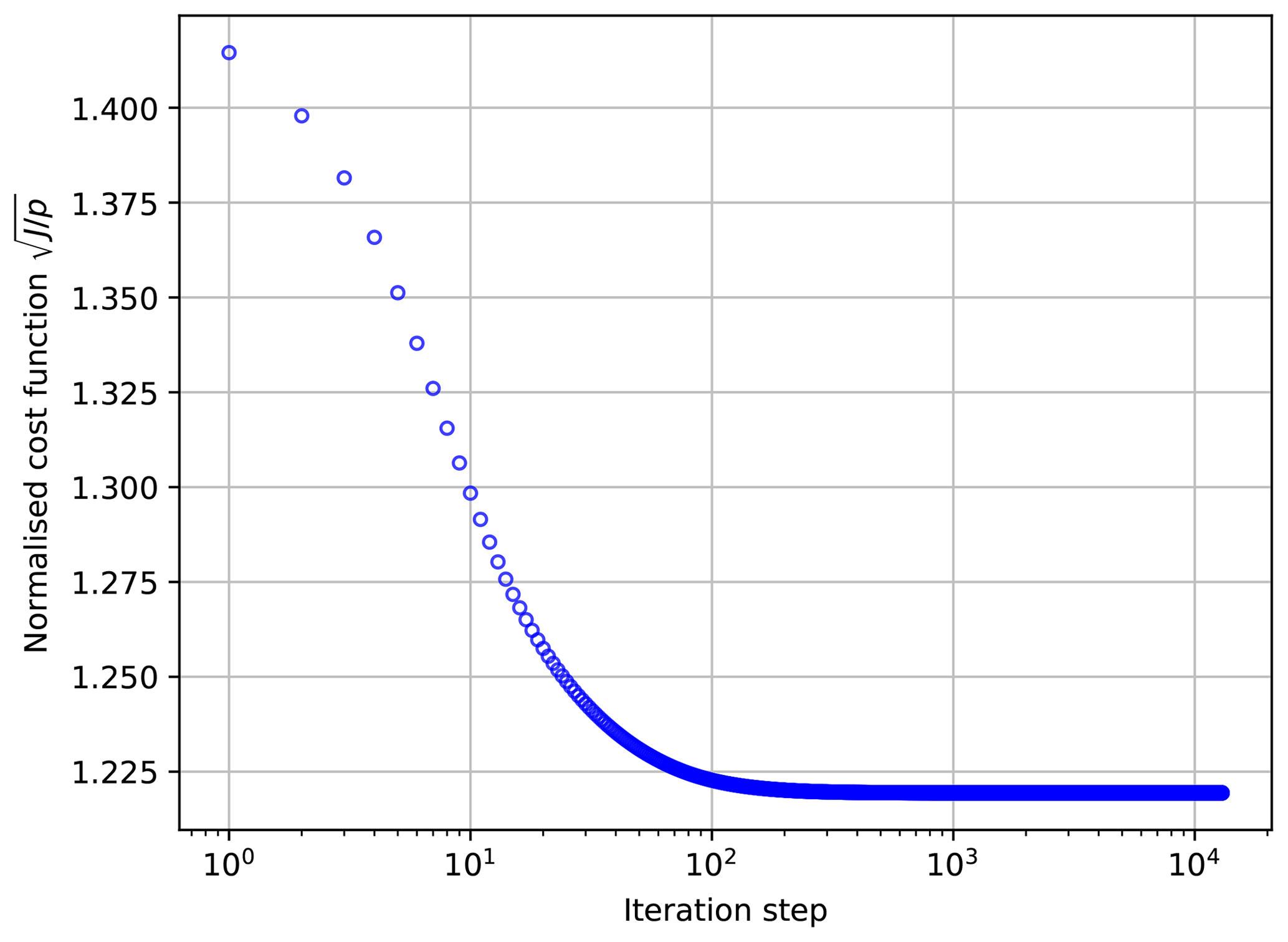
Figure 1 Iterative approach to minimise the GNC cost function J subject to the non-negativity constraints. Under the multiplicative updates in Eq. (17) the cost function decreases monotonically. In this particular example, the convergence required more than 10⁴ iterative steps.

2.3 The GIG method

Bishop (2016) introduced a variation of the ensemble Kalman filter (EnKF) that solves the univariate Bayes' theorem for non-negative variables with skewed (asymmetrical) probability distributions. The so-called GIGG-EnKF (with GIGG standing for gamma, inverse-gamma, and Gaussian) allows non-negative variables typically involving near-zero values (i.e. with right-skewed probability distributions), such as aerosol, water vapour, cloud, and precipitation concentrations, to be directly assimilated, thus avoiding the use of Gaussian anamorphosis non-linear transformations (e.g. Amezcua and Leeuwen, 2014). The GIGG-EnKF algorithm is based on the generalised two-stage multivariate ensemble filter described by Anderson (2003). The first stage involves the univariate GIGG-EnKF in which an ensemble-based estimate of the posterior distribution of the observed variable is generated from a single observation and a prior ensemble of state estimates. In the second stage, the univariate method is extended by propagating this information to the complete model state vector using a linear regression approximation.

According to the strategy proposed by Bishop (2016), in the first step, Bayes' theorem is solved in the univariate form of Eq. (7) assuming a distribution pair for the prior probability and the likelihood PDF of the error-prone observations given the truth, respectively. A single observation is assimilated using an appropriate equation set depending on three different cases: GIG, IGG, and G. The GIG equation set is aimed at situations in which the prior can be described by a gamma distribution and the observation likelihood can be represented by an inverse-gamma distribution. In addition, Bishop (2016) introduced the IGG equation set (inverse-gamma prior and gamma observation likelihood) and the G equation set (Gaussian distributions). Volcanic aerosols have been found to be well-approximated by gamma distributions (Mingari et al., 2022b). Similarly, it is shown in this paper that the prior distributions of deposit mass loading can be well-represented to some extent by gamma distributions (see Sect. 3.4). Consequently, this paper will focus exclusively on the GIG case. In the GIG case, the posterior probability is given by a gamma PDF:

$$\begin{array}{}\text{(18)}& P\left(y_j|y_j^{\mathrm{o}}\right)\propto y_j^{{\left({\mathrm{\Pi }}_j^{\mathrm{r}}\right)}^{-\mathrm{1}}-\mathrm{1}}\exp \left\{-{\displaystyle \frac{y_j}{{\mathrm{\Pi }}_j^{\mathrm{r}}{\stackrel{\mathrm{‾}}{y}}_j^{\mathrm{a}}}}\right\},\end{array}$$

where y_j and $y_j^{\mathrm{o}}$ are the jth components of the vectors y and y^o, respectively. The posterior univariate gamma PDF is characterised by two parameters, namely the analysis mean ${\stackrel{\mathrm{‾}}{y}}_j^{\mathrm{a}}$ and the type 1 relative error variance of the analysis ${\mathrm{\Pi }}_j^{\mathrm{r}}:=\mathrm{var}\left(y_j^{\mathrm{a}}\right)/({\stackrel{\mathrm{‾}}{y}}_j^{\mathrm{a}}{)}^{\mathrm{2}}$, that in the GIG method are given by

$$\begin{array}{}\text{(19a)}& {\displaystyle \frac{\mathrm{1}}{{\stackrel{\mathrm{‾}}{y}}_j^{\mathrm{a}}}}& {\displaystyle }={\displaystyle \frac{\mathrm{1}}{{\stackrel{\mathrm{‾}}{y}}_j^f}}+{\displaystyle \frac{{\stackrel{\mathrm{̃}}{P}}_j^{\mathrm{r}}}{{\stackrel{\mathrm{̃}}{R}}_j^{\mathrm{r}}+{\stackrel{\mathrm{̃}}{P}}_j^{\mathrm{r}}}}\left\{{\displaystyle \frac{\mathrm{1}}{y_j^o}}-\left({\stackrel{\mathrm{̃}}{R}}_j^{\mathrm{r}}+\mathrm{1}\right){\displaystyle \frac{\mathrm{1}}{{\stackrel{\mathrm{‾}}{y}}_j^f}}\right\},\text{(19b)}& {\displaystyle }{\left({\mathrm{\Pi }}_j^{\mathrm{r}}\right)}^{-\mathrm{1}}& {\displaystyle }={\left({\stackrel{\mathrm{̃}}{R}}_j^{\mathrm{r}}\right)}^{-\mathrm{1}}+{\left({\stackrel{\mathrm{̃}}{P}}_j^{\mathrm{r}}\right)}^{-\mathrm{1}},\end{array}$$

where ${\stackrel{\mathrm{̃}}{P}}_j^{\mathrm{r}}$ and ${\stackrel{\mathrm{̃}}{R}}_j^{\mathrm{r}}$ are the type 2 relative error variance of the prior and observations, respectively (see Table A1 in the Appendix for details).

In order to generate an analysis ensemble $y_{ji}^{\mathrm{a}}$ with the low-order moments of the posterior distribution being consistent with Eqs. (19a) and (19b), Bishop (2016) provides the following stochastic equation for the case of a univariate gamma prior and inverse-gamma observation-likelihood PDFs.

$$\begin{array}{}\text{(20)}& \begin{array}{rl}& {\displaystyle \frac{y_{ji}^{\mathrm{a}}-{\stackrel{\mathrm{‾}}{y}}_j^{\mathrm{a}}}{{\stackrel{\mathrm{‾}}{y}}_j^{\mathrm{a}}}}={\displaystyle \frac{y_{ji}^f-{\stackrel{\mathrm{‾}}{y}}_j^f}{\sqrt{{\left({\stackrel{\mathrm{‾}}{y}}_j^f\right)}^{\mathrm{2}}+\mathrm{var}\left(y_{ji}^f\right)}}}+{\stackrel{\mathrm{̃}}{P}}_j^{\mathrm{r}}{\left({\stackrel{\mathrm{̃}}{P}}_j^{\mathrm{r}}+{\stackrel{\mathrm{̃}}{R}}_j^{\mathrm{r}}\right)}^{-\mathrm{1}}\times \\ & \times \left\{{\displaystyle \frac{z_{ji}-{\stackrel{\mathrm{‾}}{z}}_j}{\sqrt{{\left({\stackrel{\mathrm{‾}}{z}}_j\right)}^{\mathrm{2}}-\mathrm{2}\mathrm{var}\left(z_{ji}\right)}}}-{\displaystyle \frac{y_{ji}^f-{\stackrel{\mathrm{‾}}{y}}_j^f}{\sqrt{{\left({\stackrel{\mathrm{‾}}{y}}_j^f\right)}^{\mathrm{2}}+\mathrm{var}\left(y_{ji}^f\right)}}}\right\}\end{array}\end{array}$$

Here, ${\stackrel{\mathrm{‾}}{y}}_j^{\mathrm{a}}$ can be computed using Eq. (19a). Equation (20) ensures that the analysis ensemble $y_{ji}^{\mathrm{a}}$ is consistent with the type 1 relative error variance of the posterior given by Eq. (19b) provided z_ji is randomly sampled from a gamma PDF with type 1 relative error variance $R_j^z$ and mean ${\stackrel{\mathrm{‾}}{z}}_j$ given by

$$\begin{array}{}\text{(21a)}& {\displaystyle }{\left(R_j^z\right)}^{-\mathrm{1}}& {\displaystyle }={\left({\stackrel{\mathrm{̃}}{R}}_j^{\mathrm{r}}\right)}^{-\mathrm{1}}+\mathrm{2},\text{(21b)}& {\displaystyle }{\stackrel{\mathrm{‾}}{z}}_j& {\displaystyle }={\displaystyle \frac{{\left({\stackrel{\mathrm{̃}}{R}}_j^{\mathrm{r}}\right)}^{-\mathrm{1}}+\mathrm{2}}{{\left({\stackrel{\mathrm{̃}}{R}}_j^{\mathrm{r}}\right)}^{-\mathrm{1}}}}{y}_j^{\mathrm{o}}.\end{array}$$

In addition, the ensemble generated in this way is ensured to converge to the true posterior PDF for large ensembles.

The univariate case is extended according to the second-stage linear regression step proposed by Anderson (2003) in order to find the analysis ensemble for the complete model state vector. The update of the kth model state vector variable of the ith ensemble member due to the jth observation is computed according to

$$\begin{array}{}\text{(22)}& x_{ki}^{\mathrm{a}}=x_{ki}^f+{\displaystyle \frac{\mathrm{cov}\left(x_k^f,y_j^f\right)}{\mathrm{var}\left(y_j^f\right)}}\left(y_{ji}^{\mathrm{a}}-y_{ji}^f\right).\end{array}$$

The inverse-gamma PDFs assign non-zero probability densities only for positive observations, and, as a result, zero observations cannot be properly assimilated using the GIG equation set (see e.g. Eq. 19a). This problem is addressed here by redefining zero observation data according to

$$\begin{array}{}\text{(23)}& y_j^{\mathrm{o}}\leftarrow r\times {\mathit{ϵ}}_{min},\end{array}$$

where $r\in (\mathrm{0},\mathrm{1}]$ is a random number and ϵ_min is a typical error expected for zero-valued observations of deposit thickness (assumed to be ϵ_min = 1 mm in this work since only visible tephra deposits are considered here).

The GIG method is a sequential procedure: a single observation is assimilated in order to update the prior ensemble forecast using the GIG equation set; subsequently, this procedure is repeated until all observations have been sequentially assimilated. In contrast, the GNC method described in Sec. 2.2 represents an all-at-once assimilation technique. Another important difference is that the GIG method is stochastic; i.e. different applications of the method will lead to different realisations of the analysis. To summarise, a pseudocode of the sequential procedure used to implement the GIG method is detailed in Algorithm 1.

Algorithm 1 Pseudocode of the GIG method based on the Bishop (2016) algorithm for the case in which the prior is a gamma distribution and the observation likelihood is an inverse-gamma distribution.

Require:

List of observations $\mathit{\left\{}{y}_j^{\mathrm{o}}\mathit{\right\}}$ with their relative errors

Ensure:

Analysis ensemble $x_{ki}^{\mathrm{a}}$

1:

get $x_{ki}^f$

▹Generate the prior ensemble

2:

procedure GIG Method

3:

randomly shuffle observation list

4:

for all $y_j^{\mathrm{o}}$ do

▹Iterate over observations

5:

if $y_j^{\mathrm{o}}=\mathrm{0}$ then

6:

$r\leftarrow \text{random number}\in (\mathrm{0},\mathrm{1}]$

7:

$y_j^{\mathrm{o}}\leftarrow r*{\mathit{ϵ}}_{min}$

▹Redefine zero observations

8:

end if

9:

${\stackrel{\mathrm{‾}}{y}}_j^{\mathrm{a}}\leftarrow$ Eq. (19a)

10:

$y_{ji}^{\mathrm{a}}\leftarrow$ Eq. (20)

11:

$x_{ki}^{\mathrm{a}}\leftarrow$ Eq. (22)

▹Generate the analysis ensemble

12:

$x_{ki}^f\leftarrow x_{ki}^{\mathrm{a}}$

▹Update the prior ensemble

13:

end for

14:

end procedure

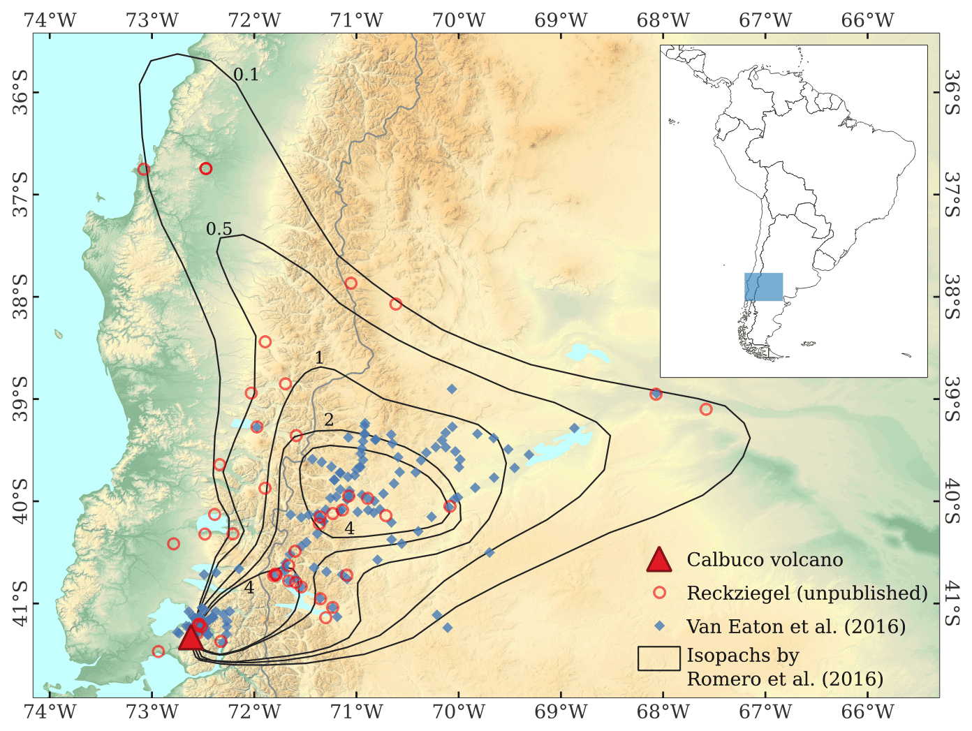
Figure 2 Location of the sampling sites corresponding to the dataset reported by Van Eaton et al. (2016) (blue diamond) and an independent dataset composed of 45 measurements (red circle) provided by Florencia Reckziegel (personal communication, September 2020). The map also shows the isopachs of fall deposit thickness in millimetres reported by Romero et al. (2016) used for validation purposes in this work.

3 Reconstruction of the 2015 Calbuco deposit

In this section, the procedures described in Sect. 2 are applied to the 2015 Calbuco eruption in order to obtain the analysed deposit thickness. With this in mind, a total of 204 field measurements of deposit thickness will be considered for assimilation and validation purposes. This dataset is composed of 160 measurements reported by Van Eaton et al. (2016) and an independent dataset of 44 measurements provided by Florencia Reckziegel (personal communication, September 2020). Figure 2 shows the location of the sampling sites for both datasets.

3.1 Fallout deposit and datasets

The 2015 eruption of the Calbuco stratovolcano (41.33^∘ S, 72.61^∘ W) in southern Chile involved two major eruptive pulses on 22–23 April along with a third minor pulse on 30 April (Romero et al., 2016). During the most energetic phase on 23 April, stratospheric eruption columns higher than 15 km above the vent level (∼ 17 km above sea level) were developed. Regions over southern Chile and the Argentinian Patagonia were severely affected by tephra fall. According to different estimations based on field studies, deposit volume ranges between 0.27 and 0.58 km³ (Romero et al., 2016; Van Eaton et al., 2016).

The availability of independent and comprehensive datasets of field observations makes the Calbuco tephra deposit an excellent case study. Van Eaton et al. (2016) reported the thickness and stratigraphy of the fall deposits at 163 sampling sites within a 500 km radius from the volcano summit. In addition, a complementary dataset composed of 45 independent measurements of deposit thickness (Florencia Reckziegel, personal communication) distributed over a larger region is also available (Fig. 2). Finally, a hand-drawn isopach map built from a third independent dataset (Romero et al., 2016) is also used to evaluate the tephra deposit distribution. The corresponding isopachs for 0.1, 0.5, 1.0, 2.0, and 4 mm are represented in Fig. 2. The three datasets are summarised in Table 1.

Van Eaton et al. (2016)Romero et al. (2016)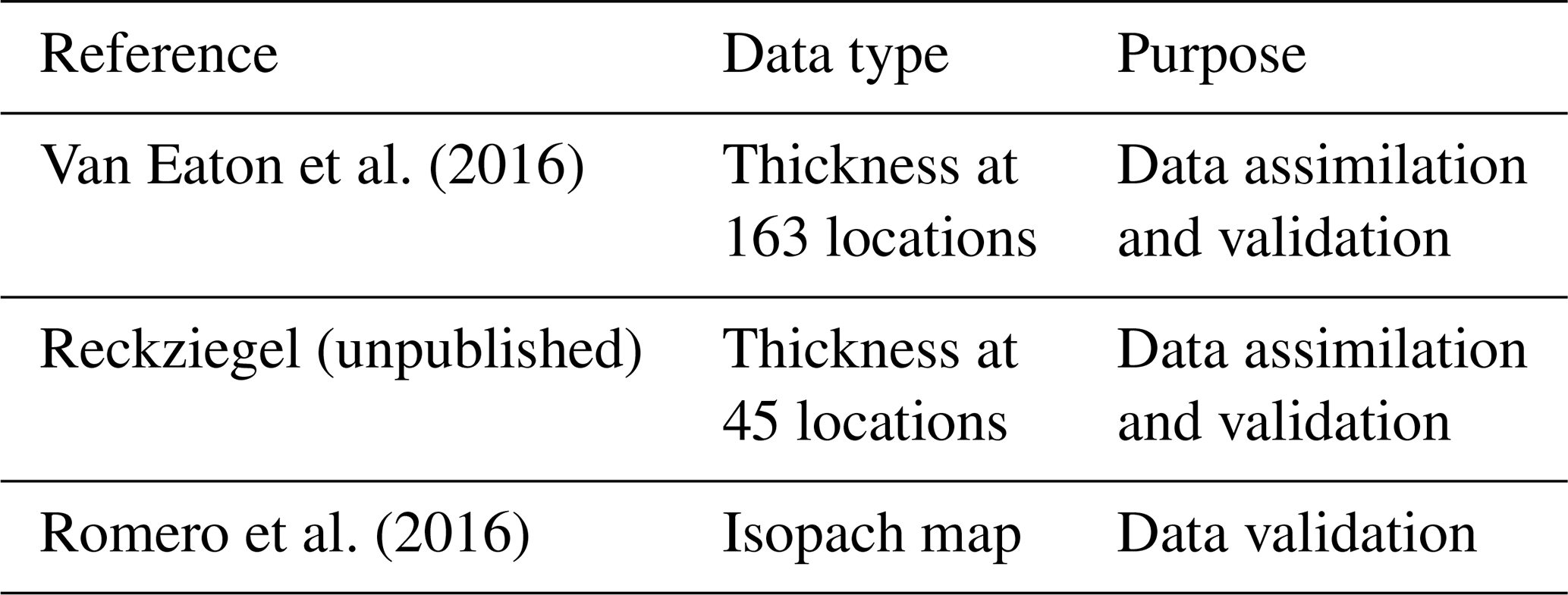

Table 1 Calbuco deposit datasets considered in this study.

It is interesting to note the presence of a secondary thickness maximum ∼ 200 km downwind from the vent, located around two major cities of the Argentinian Patagonia, Junín de los Andes (39.95^∘ S, 71.07^∘ W) and San Martín de los Andes (40.16^∘ S, 71.35^∘ W), likely due to ash aggregation processes (e.g. Costa et al., 2010). The emergence of this distal maximum indicates that complex plume dynamics were involved in the volcanic eruption.

The assimilation methods require a dataset of measurements along with the corresponding absolute or relative errors. Specifically, the GNC method requires the absolute error ϵ_j associated with the jth measurement $y_j^{\mathrm{o}}$ (the observation error covariance matrix R is assumed to be diagonal with elements ${\mathit{ϵ}}_j^{\mathrm{2}}$). On the other hand, the GIG method requires the relative error ${\mathit{ϵ}}_j^{\mathrm{r}}={\mathit{ϵ}}_j/y_j^{\mathrm{t}}$, where $y_j^{\mathrm{t}}$ is the true value of the jth observation.

The strategy adopted in this work to provide reasonable error estimates is based on a clustering algorithm, and observation error standard deviations are assumed to be dependent on the measured value. In summary, observational data are organised into groups with similar characteristics, and an absolute and relative error is assigned to each group or cluster. The error for the jth measurement $y_j^{\mathrm{o}}$ is approximated by the standard deviation associated with the corresponding cluster; the true value $y_j^{\mathrm{t}}$, required to estimate relative errors, is approximated by the cluster mean value. A more detailed explanation of the strategy used to estimate errors can be found in the Supplement.

3.2 Validation metrics

As validation metrics, we consider the weighted versions of the mean bias error (MBE) and the root mean square error (RMSE) to measure the differences between observations and analyses, defined as

$$\begin{array}{}\text{(24a)}& {\displaystyle }\mathrm{MBE}& {\displaystyle }={\displaystyle \frac{\mathrm{1}}{p}}\sum _{j=\mathrm{1}}^p{\mathit{\omega }}_i\left(y_j^{\mathrm{o}}-y_j\right),\text{(24b)}& {\displaystyle }\mathrm{RMSE}& {\displaystyle }=\sqrt{{\displaystyle \frac{\mathrm{1}}{p}}\sum _{j=\mathrm{1}}^p{\mathit{\omega }}_i^{\mathrm{2}}{\left(y_j^{\mathrm{o}}-y_j\right)}^{\mathrm{2}}}.\end{array}$$

Notice that if the non-weighted (ω_j=1) versions of Eq. (24b) are used, the MBE (in cm) quantifies the tendency to overestimate or underestimate observations for the overall dataset, whereas the RMSE (in cm) measures the average magnitude of the errors. These two metrics are suitable when a uniform distribution of errors is expected. However, the datasets in this work contain measurements spanning 4 orders of magnitude, and the assumption of a constant absolute error seems to be inappropriate in this case because only proximal data (i.e. the largest measurements of deposit thickness) contribute significantly to the non-weighted versions of MBE and RMSE. Instead, in order to treat the deviations more evenly, the observation uncertainties are used to define the weights according to ${\mathit{\omega }}_j=\mathrm{1}/{\mathit{ϵ}}_j$. These weighted versions of MBE and RMSE represent dimensionless evaluation metrics, and the impact of the assimilation can be better characterised by means of these metrics. Ideally, the MBE should be close to zero and RMSE should be close to 1.

Another relative metric used to evaluate the deposit reconstruction is the symmetric mean absolute percentage error (SMAPE), defined as

$$\begin{array}{}\text{(25)}& \mathrm{SMAPE}=\mathrm{100}\times {\displaystyle \frac{\mathrm{2}}{p}}\sum _{j=\mathrm{1}}^p{\displaystyle \frac{|y_j^o-y_j|}{\left|y_j^o\right|+\left|y_j\right|}},\end{array}$$

and is expressed in percentages. Notice that this metric does not depend on the observation errors.

3.3 Ensemble modelling

Numerical simulations were carried out using the latest version release of FALL3D (v8.2), an open-source offline Eulerian model for atmospheric transport and deposition of aerosols and particles, including tephra species. FALL3D solves the so-called advection–diffusion–sedimentation (ADS) equation (Folch et al., 2020; Prata et al., 2021). The new FALL3D version has been designed to support increasingly larger scientific workloads and prepare the code for the transition to extreme-scale computing systems (Folch et al., 2023). Specifically, the code version v8.x has been released with several improvements over previous versions, including improvements in the model physics, numerical algorithmic methods, and computational efficiency. In addition, from version v8.1 onwards, the FALL3D model enables ensemble simulations to be performed very efficiently by means of a single parallel task (Folch et al., 2022b). Ensemble modelling allows one to characterise and quantify model uncertainties due to poorly constrained input parameters and errors in the model physics parameterisations or the underlying model-driving meteorological data. In addition, the ability to generate ensemble runs makes it possible to improve forecasts by incorporating observations using different ensemble-based data assimilation techniques.

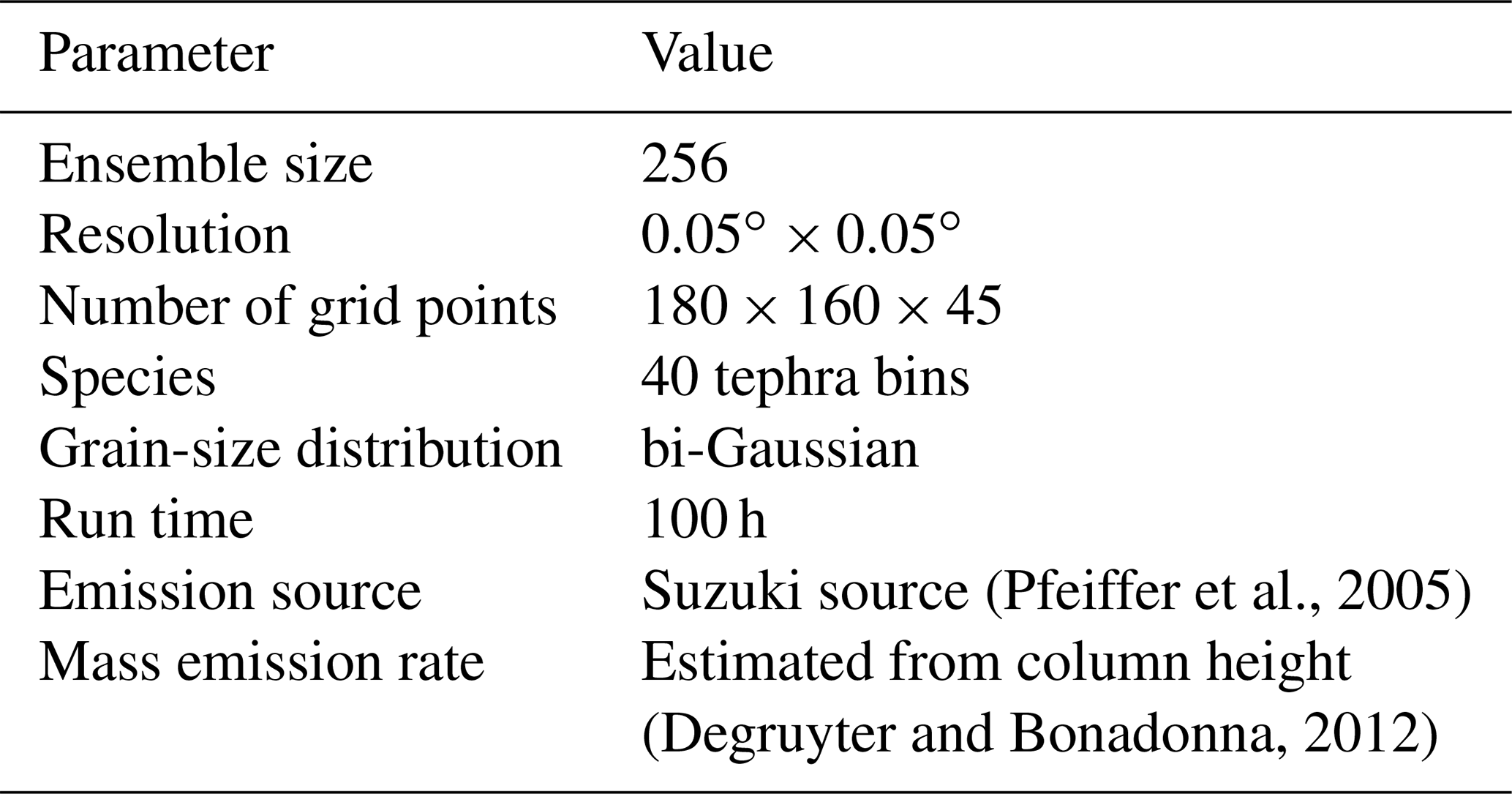
The configuration of the FALL3D model used in this work is summarised in Table 2. A three-dimensional computational domain with a horizontal resolution of ∼ 4 km (0.05^∘) and 180 × 160 × 45 grid points was defined. The total grain-size distribution (TGSD) of tephra injected into the atmosphere consists of the sum of two log-normal distributions (i.e. bi-Gaussian in Φ units) including 40 tephra bins. The modes and standard deviations of the bimodal distribution were computed using the parameterisation proposed by Costa et al. (2016), which estimates them from the eruption intensity and magma viscosity. The mode of the coarser population was located at −1.2Φ with a standard deviation of 1.71 Φ, while the mode of the finer population was 3.49 Φ with a standard deviation of 1.46 Φ. The weight of each subpopulation was set to p_c=0.15 and p_f=0.85 for the coarse and fine population, respectively. The vertical mass distribution of the source term depends on the eruptive column-top height (H) according to the following parameterisation (Pfeiffer et al., 2005):

$$\begin{array}{}\text{(26)}& {\displaystyle \frac{\mathrm{d}m}{\mathrm{d}z}}\propto {\left\{\left(\mathrm{1}-{\displaystyle \frac{z}{\mathbf{H}}}\right)\exp \left[A_{\mathrm{s}}\left({\displaystyle \frac{z}{\mathbf{H}}}-\mathrm{1}\right)\right]\right\}}^{{\mathit{\lambda }}_{\mathrm{s}}},\end{array}$$

where A_s and λ_s are the so-called Suzuki parameters (Suzuki, 1983; Pfeiffer et al., 2005). Finally, the mass emission rate was computed from the eruptive column-top height using the relationship proposed by Degruyter and Bonadonna (2012).

(Pfeiffer et al., 2005)(Degruyter and Bonadonna, 2012)

Table 2 FALL3D model configuration parameters for the 2015 Calbuco runs.

A 256-member prior ensemble was generated by perturbing the eruption source parameters (ESPs) and the horizontal wind components around a reference value using either uniform or truncated normal distributions. Table 3 lists the perturbed model parameters along with the corresponding reference values and sampling uncertainty ranges. Latin hypercube sampling (LHS, McKay et al., 1979) was used to efficiently sample the parameter space. Two eruptive phases were considered with reference values of column-top heights at H = 15 $\mathrm{km}\mathrm{a}.\mathrm{v}.\mathrm{l}.$ (above vent level) for each phase. The column-top height H was independently perturbed for each phase assuming a sampling range of ± 25 %. The source start time for the central member was defined at 21:00 UTC on 22 April 2015 (first phase) and at 04:00 UTC on 23 April 2015 (second phase) assuming a duration of 1.6 and 6 h for each phase. Source start times and phase duration were also perturbed.

Table 3 Ensemble configuration. The perturbed model parameters are eruption column height (H), eruption phase start time (T_i), phase duration (ΔT), parameters A_s and λ_s of the Suzuki vertical mass distribution, the fine mode of the bi-Gaussian TGSD, the density of aggregates, and the wind components.

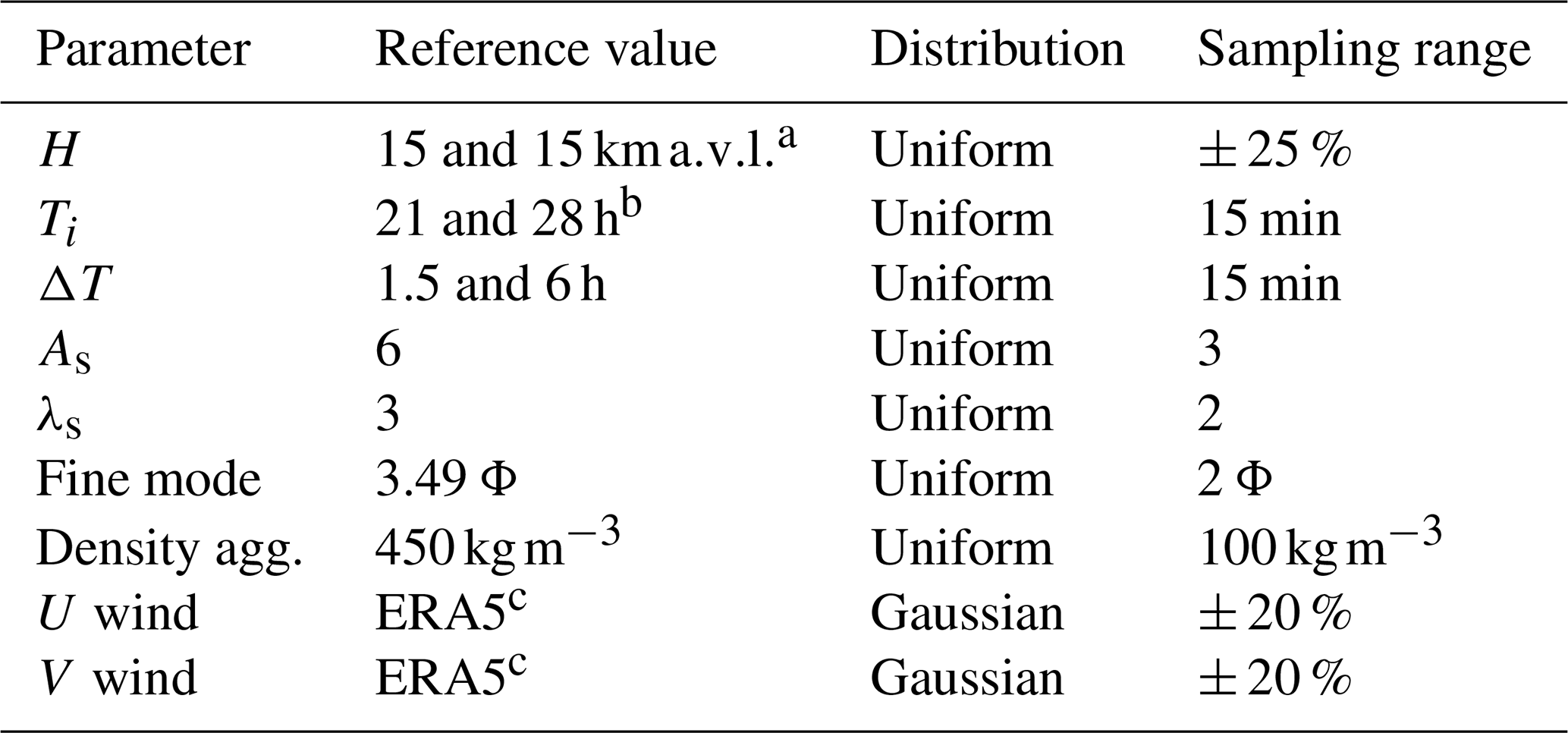
^a Two eruptive phases are considered. Heights are given in kilometres above the vent level. ^b Hours since 22 April 2015 at 00:00 UTC. ^c ECMWF atmospheric reanalysis (137 model levels).

3.4 Prior ensemble distribution

Before showing how the assimilation methods perform, it is worth characterising the prior ensemble distribution and checking whether the assumptions of the GIG method are fulfilled (i.e. the prior distribution can be approximated by a gamma PDF). To this purpose, the skewness ${\stackrel{\mathrm{̃}}{\mathit{\mu }}}_{\mathrm{3}}$ (i.e. the third standardised moment, ${\mathit{\mu }}_{\mathrm{3}}/{\mathit{\sigma }}^{\mathrm{3}}$) of the prior distribution was computed from the random samples $y_{ji}^f$, i.e. the forecasted deposit thickness according to the ith ensemble member (i=1…m) at the sampling site of the jth observation (j=1…p). Figure 3 shows the results for each observation point by plotting ${\stackrel{\mathrm{̃}}{\mathit{\mu }}}_{\mathrm{3}}$ as a function of the ratio of the standard deviation to the mean, i.e. $\sqrt{P_j^{\mathrm{r}}}$ (using the notation introduced in Sect. 2.3). For illustrative purposes, the skewness of three different theoretical distributions (Gaussian, log-normal, and gamma) is shown. As expected, the symmetric Gaussian distribution, characterised by ${\stackrel{\mathrm{̃}}{\mathit{\mu }}}_{\mathrm{3}}=\mathrm{0}$, does not reproduce the positively skewed prior distribution. The log-normal family of probability distributions represents an example of distributions for positive-definite variables with a lower bound. However, as shown in Fig. 3, the log-normal distribution cannot properly represent the prior distribution because the theoretical skewness is extremely large in this case. In contrast, the skewness computed from the prior distributions (blue dots) is well-approximated by the relationship ${\stackrel{\mathrm{̃}}{\mathit{\mu }}}_{\mathrm{3}}=\mathrm{2}\sqrt{P_j^{\mathrm{r}}}$, which is the theoretical expression corresponding to the gamma distribution (solid black line).

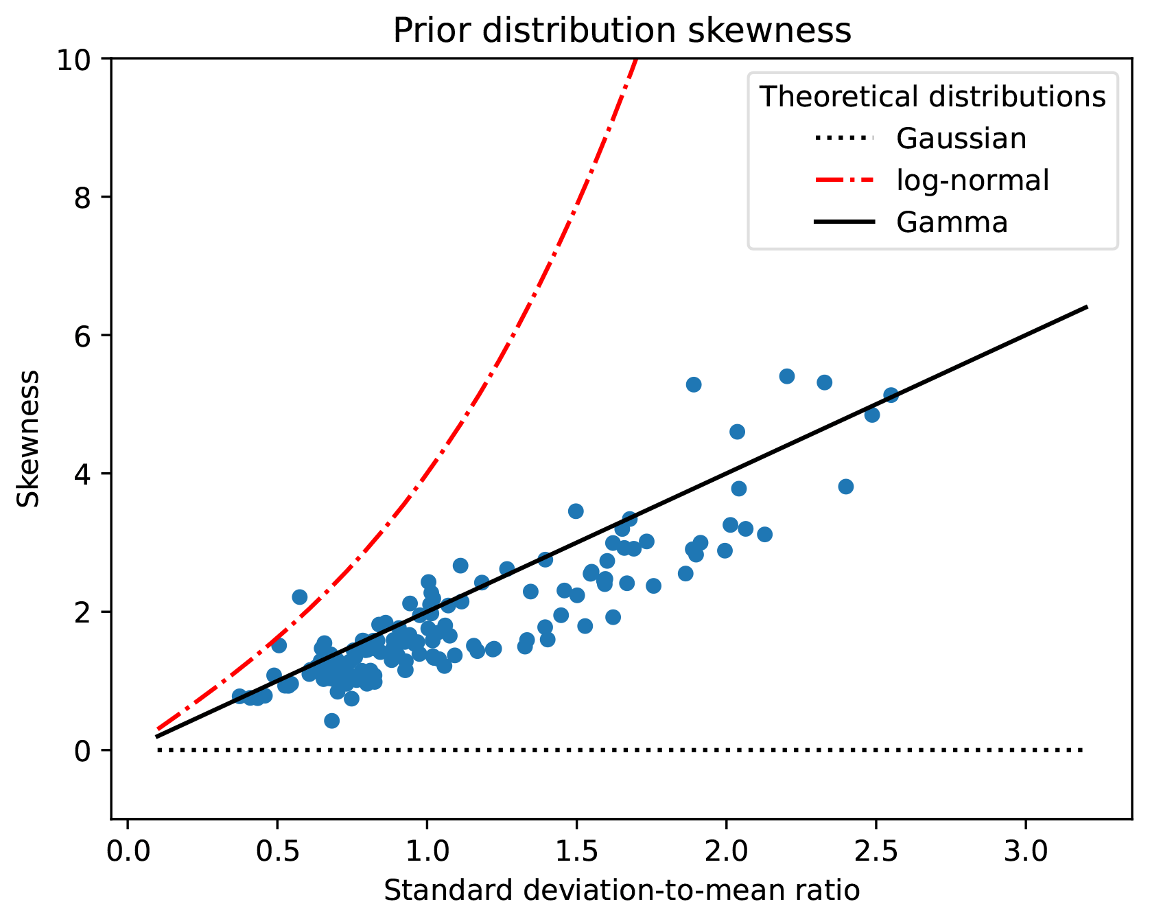
Figure 3 Skewness as a function of the ratio of the standard deviation to the mean for the prior distribution at the sampling locations (blue circles). Results for some theoretical distributions (Gaussian, log-normal, and gamma) are also shown for comparison.

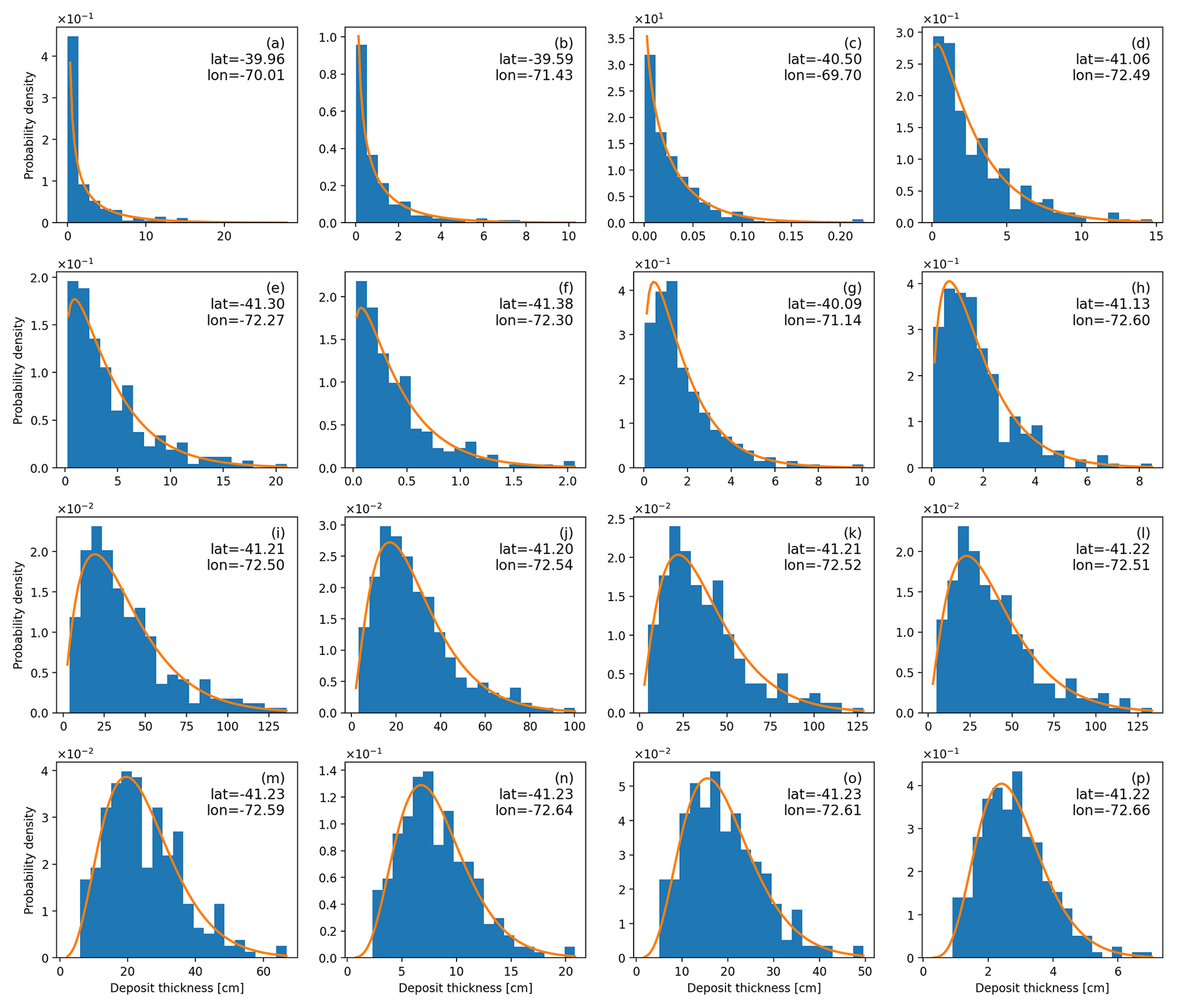
Figure 4 Histograms of sampled prior distributions along with the corresponding theoretical gamma distribution (solid line) at some selected observation sites.

In order to further understand the similarities between the gamma and prior distributions, Fig. 4 explicitly shows histograms of sampled prior distributions along with the corresponding theoretical gamma distribution for some observation sites. The theoretical gamma distributions were constructed using the sampled first and second moments. As observed, good agreement is found between the two distributions in almost all cases. Note that when the type 1 relative error variance is greater than 1 ($P_j^{\mathrm{r}}>\mathrm{1}$) the gamma probability density decreases monotonically (Fig. 4a–c) and the mode becomes zero. In contrast, when $P_j^{\mathrm{r}}<\mathrm{1}$ or, equivalently, when ${\stackrel{\mathrm{‾}}{y}}_j^{\mathrm{2}}>\mathrm{var}\left(y_j\right)$, the mode becomes positive (Fig. 4d–p). The results obtained is this section justify the suitability of the GIG method to deal with the assimilation of volcanic deposit data.

3.5 Analyses

In this section, we compare the tephra deposit field reconstructed according to four strategies: (i) forecast, i.e. the prior ensemble mean, (ii) the EnKF method, i.e. the analysis ensemble mean via Eq. (5a), (iii) the GNC method, and (iv) the GIG method. Notice that the GNC method gives a set of weight factors for each ensemble member w_i ($i=\mathrm{1},\mathrm{\dots },m$), and the best estimate of the system state is obtained by replacing the optimal weight factors in Eq. (11). On the other hand, the GIG method produces an ensemble of analysis states and the analysis ensemble mean is used for comparison purposes in this section. The full dataset of 204 measurements was assimilated to compute the analysis according to strategies (ii)–(iv).

The results of the tephra fall deposit reconstruction are shown in Fig. 5. For comparative purposes, the Romero et al. (2016) deposit contours (hand-drawn isopachs for 0.1, 0.5, 1, 2, and 4 mm) are superimposed in Fig. 5. These contours are based on an independent dataset of thickness measurements (different from the assimilation dataset). The presence of the distal secondary thickness maximum was reproduced by the reconstructed deposits taking into account the ash aggregation processes in the numerical simulation. To this purpose, the parameterisation proposed (Cornell et al., 1983; Folch et al., 2010) was used assuming an aggregate particle class having a diameter of 200 µm and a density sampled in a range centred around 450 kg m⁻³ (see Table 3).

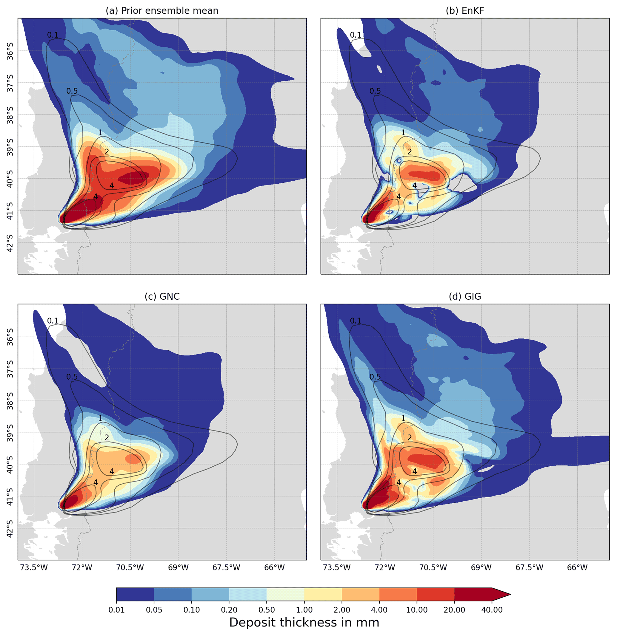
Figure 5 Reconstructed tephra fall deposit according to the forecast (a), EnKF method (b), GNC method (c), and GIG method (d). The Romero et al. (2016) deposit contours (isopachs for 0.1, 0.5, 1, 2, and 4 mm) are also superimposed for comparative purposes.

The forecast (Fig. 5a) indicates an excessively high deposited mass. In particular, the 2 and 4 mm contours are overestimated by almost an order of magnitude. This is corrected by the three methods (Fig. 5b and c), which yield analyses with reduced total mass on the ground.

The EnKF analysis shows a very noisy spatial distribution with large oscillations and negative values in some regions, leading to artificial spatial structures. On the other hand, the GNC shows smoother deposit thickness contours with a spatial distribution having a more physically plausible structure. The GIG method represents an intermediate case between the EnKF and GNC methods. Although this method gives unrealistic results as well, the fraction of negative values and the amplitude of oscillations are noticeably reduced compared to the EnKF method (negative data were remove and reassigned to zero).

3.6 Validation

In order to evaluate the performance of the analysis schemes, the full dataset of observations was split into two subsets: an assimilation dataset and a validation dataset. The assimilation dataset was used to produce new analyses, and the validation metrics defined in Sect. 3.2 were computed for the validation dataset. This methodology ensures that validation is done against non-assimilated observations. However, the validation metrics will be meaningless if the assimilation and validation datasets are strongly correlated (e.g. if measurement sites are very close to each other). The splitting procedure aims to reduce the correlation between the two subsets and is described in the Supplement.

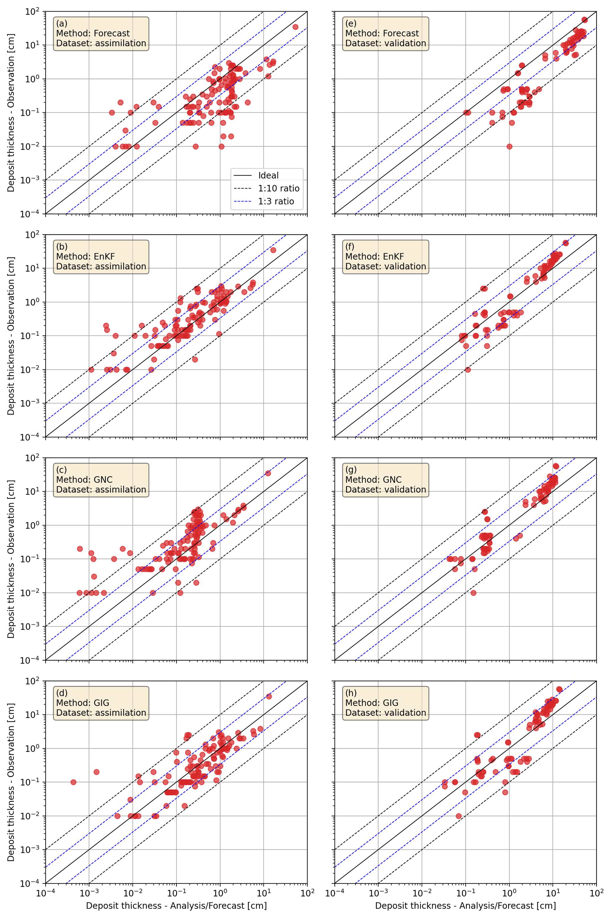
Figure 6 Comparison between analyses and observations for the forecast (a, e), EnKF (b, f), GNC (c, g), and GIG (d, h) methods. Panels in the left column (a–d) present the assimilation dataset (60 % of the full dataset), and the validation dataset (40 % of the full dataset) is shown in the right column (e–h).

Figure 6 compares the analysis results at each sampling site with observations from the assimilation dataset (Fig. 6a–d) and the validation dataset (Fig. 6e–h) considering a dataset partition of 60 % and 40 %, respectively. The forecast systematically overestimates observations (Fig. 6a and e), as already noted in Sect. 3.5. Since measurements span a range of 4 orders of magnitude between 10⁻² and 10² cm, good agreement for the entire range of data values turns out to be challenging. Nevertheless, results for the analyses corresponding to EnKF (Fig. 6b and f), GNC (Fig. 6c and g), and GIG (Fig. 6d and h) methods show that most of the data lie within the 1-to-10 ratio band (black dashed lines).

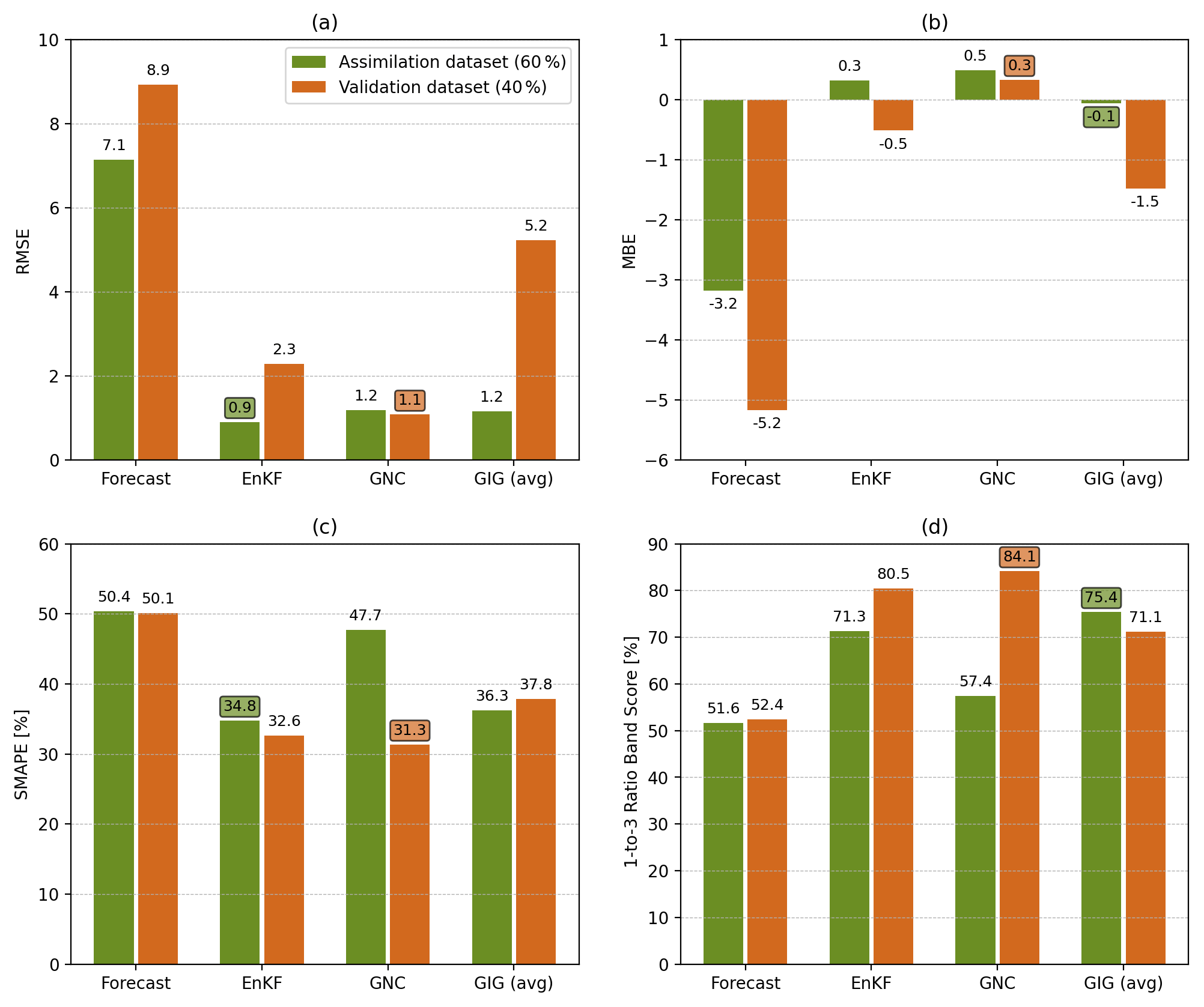
Figure 7 Evaluation metrics for the prior ensemble mean (forecast) and the EnKF, GNC, and GIG analysis schemes. The metrics were computed from the assimilation and validation datasets considering a partition of the full dataset of 60 % and 40 %, respectively.

In order to quantify deviations from observations according to the prior ensemble mean (forecast) and the analysis schemes, the evaluation metrics computed for the assimilation dataset (60 %) and the validation dataset (40 %) are reported in Fig. 7. Since the GIG method is stochastic, six realisations of the analysis were computed, and the average over the realisations are reported for each metric. The EnKF, GNC, and GIG methods improve all metrics compared to the forecast. In particular, the RMSE computed from the assimilation dataset (Fig. 7a, green bar) is reduced from 7.1 (forecast) to 0.9 (EnKF) and 1.2 (GNC, GIG). Since the EnKF provides the best estimate in terms of RMSE, this is an expected result. However, when the RMSE is computed for the validation dataset (Fig. 7a, brown bar), the performance of EnKF (2.3) and GIG (5.2) methods degrades significantly, and the best performance is achieved by the GNC method (1.1). Note that this result is very close to the ideal value RMSE = 1, meaning that deviations are similar to the observation uncertainty (see Eq. 24b).

The bias is presented in Fig. 7b. The GNC MBE (0.3) is positive, meaning that measurements are underestimated, but this bias is within the observation uncertainty range since MBE < 1. In contrast, the analysis overestimates observations according to EnKF (MBE = −0.5) and GIG (MBE = −1.5) methods. The best SMAPE results were obtained for GNC (SMAPE = 31.8 %) and EnKF (SMAPE = 32.6 %) as shown in Fig. 7c. Finally, Fig. 7d presents the 1-to-3 ratio band score, defined as the percentage of data points within the 1-to-3 ratio band (blue dashed lines in Fig. 6). Again, the best result was obtained for the GNC method (84.1 %).

In conclusion, the GNC method outperforms the EnKF and GIG methods in term of all metrics computed for the validation dataset. In contrast, the EnKF and GIG analyses perform well over regions around the observation sites, but the analyses cannot fully capture all deposit features beyond these regions. In order to illustrate this point, the uncorrected EnKF analysis (i.e. negative data were not removed) and the location of the assimilated observations (60 % of the full dataset) are presented in Fig. 8, where colour-shaded regions represent positive data and negative data are masked. Large oscillations emerge in regions without observation data, leading to artificial structures in the deposit field. This example clearly highlights the problems arising when the EnKF is applied to this case and the importance of dealing with the assimilation of volcanic deposit data using alternative approaches.

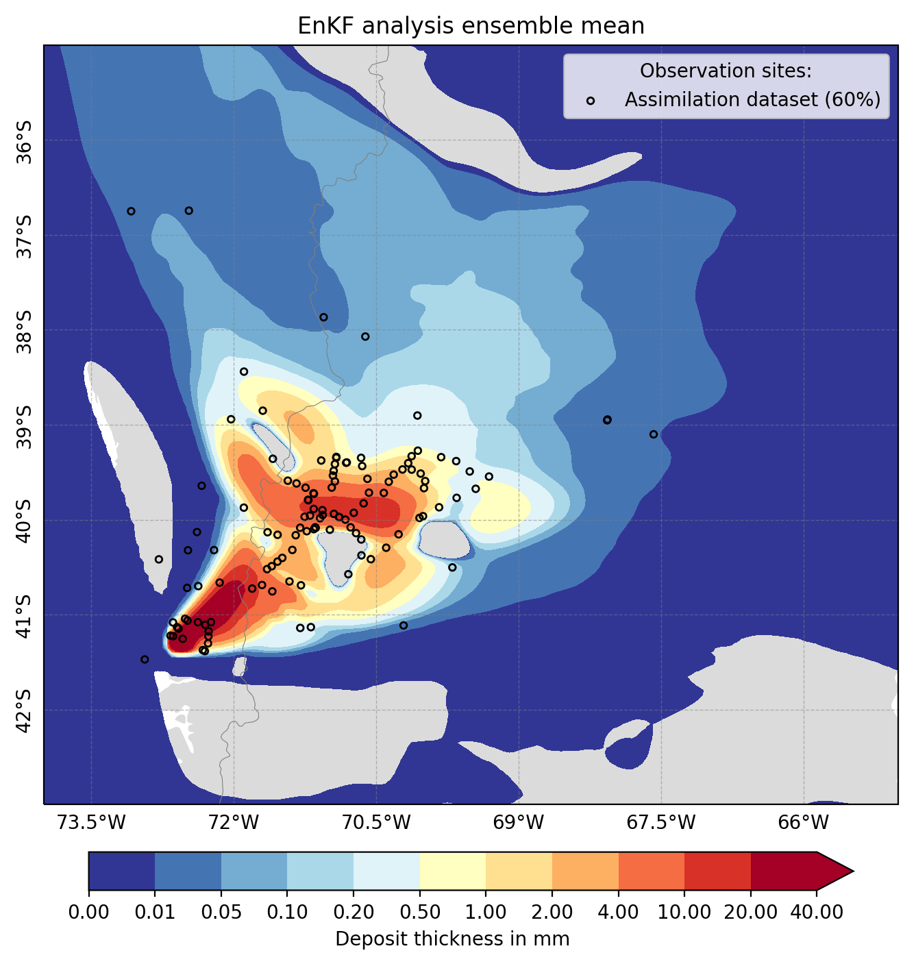
Figure 8 Tephra fall deposit according to the EnKF method and location of the assimilated observations (60 % of the full dataset). Colour-shaded regions represent positive data, and negative data are masked in order to illustrate the emergence of large oscillations and unphysical values in regions with scarce observational data.

To conclude this section, different partitions of the observational dataset are considered, and the RMSE is computed for the validation dataset. Results are shown in Fig. 9, expressed in terms of the percentage of assimilated observations for each partition. Again, the results show that the GNC outperforms the EnKF and GIG methods systematically, not just for a particular choice of the validation dataset. Unfortunately, it is not possible to conclude that the GIG method has improved the results of the EnKF analysis from the evidence presented in this paper.

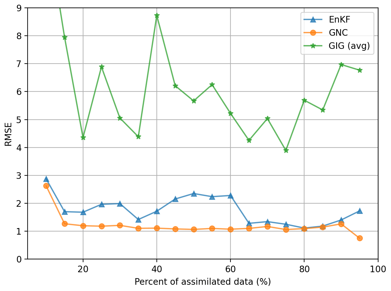
Figure 9 RMSE computed for the validation dataset for different partitions of the full dataset of observations expressed in terms of the percentage of assimilated observations.

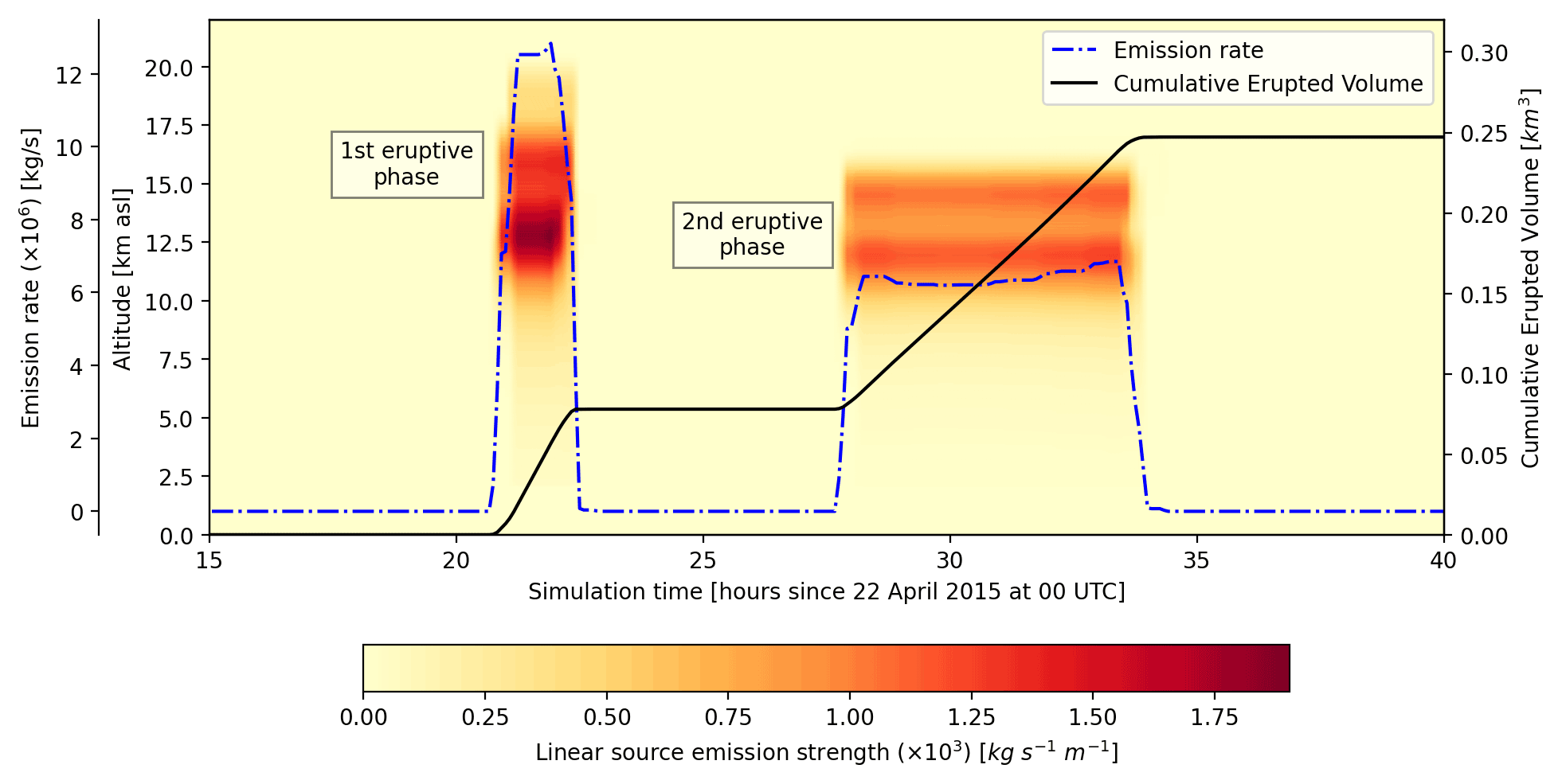
Figure 10 Profiles of emission rate and time series of eruption source parameters (ESPs) for the 2015 Calbuco eruption according to the GNC inverse modelling approach. The solid line represents the cumulative erupted volume (km³), and the dash-dotted line indicates the mass emission rate (kg s⁻¹).

4 Source term inversion: application to the 2015 Calbuco eruption

A major advantage of the GNC method is that it allows estimating the eruption source parameters (ESPs) in a straightforward way, with inverse modelling coming at no extra computational cost. This is because FALL3D solves an almost linear problem with weak non-linearity effects (e.g. due to gravity current, wet deposition, or aggregation), and consequently, a rescaling of the emission source term s_i associated with the ith ensemble member according to s_i→w_is_i leads to a deposit mass loading rescaled correspondingly, with w_i being the weight factor provided by the GNC method. In this case, the best estimation of the total source term is given by

$$\begin{array}{}\text{(27)}& s^{\mathrm{a}}=\sum _i{w}_i{s}_i,\end{array}$$

where {s_i} represents the emission source terms of the prior ensemble members (in $\mathrm{kg}{\mathrm{m}}^{-\mathrm{3}}{\mathrm{s}}^{-\mathrm{1}}$). Figure 10 shows the emission rate profiles resulting from the source inversion, expressed in terms of the linear source emission strength (in $\mathrm{kg}{\mathrm{m}}^{-\mathrm{1}}{\mathrm{s}}^{-\mathrm{1}}$), i.e. s^a×dA, where dA is the area of the grid cell.

As most of the 256 weight factors converge to zero, w_i→0, the profiles in Fig. 10 reflect only those ensemble members that effectively contribute to the analysed deposit mass loading. According to the GNC inverse modelling results, each eruptive phase is characterised by different vertical mass distribution and emission rates. The first phase results in higher cloud-top heights, reaching almost 20 $\mathrm{km}\mathrm{a}.\mathrm{s}.\mathrm{l}.$, whereas the column heights during the second phase remain at around 16 $\mathrm{km}\mathrm{a}.\mathrm{s}.\mathrm{l}.$ Also note that the prior ensemble was defined assuming the same emission source and sampling parameters for both eruptive phases. For instance, the ensemble configuration was defined assuming the same reference value for column heights, i.e. 15 km above vent level for both phases (Table 3) or approximately 17 $\mathrm{km}\mathrm{a}.\mathrm{s}.\mathrm{l}.$ Therefore, the resulting asymmetry between the two pulses observed in Fig. 10 is a consequence of the GNC inversion procedure. In other words, the GNC method can discard inappropriate ensemble members and pick out those that are consistent with observations.

The time series for mass eruption rate and total erupted volume are also depicted in Fig. 10. Although the maximum emission rate is reached during the more intense first phase, most of the total erupted mass stems from the longer second phase. In order to estimate the total erupted volume, a bulk density of ρ_b = 800 kg m⁻³ was assumed (a typical value for fresh deposits). In particular, the final total erupted volume was around 0.25 km³. According to the inversion, the erupted volumes corresponding to the first and second phases were 0.078 km³ (31.6 %) and 0.169 km³ (68.4 %), respectively. These results are in good agreement with the estimations reported by Romero et al. (2016), which give a total bulk tephra fall deposit volume of 0.27 ± 0.007 km³ with 62 % of the total volume corresponding to the second phase.

5 Discussion

Traditional ensemble-based DA methods such as the ensemble Kalman filter (EnKF) are based on the Gaussian hypothesis. However, it is well-known that analyses produced by these methods are suboptimal when either the model state variables or the observation errors are not Gaussian-distributed. Volcanic aerosol concentrations and tephra deposit mass loading are two remarkable examples of non-Gaussian-distributed variables with highly skewed distributions (Mingari et al., 2022b). This explains why the application of EnKF-like methods in VATD models often leads to non-physical results and oscillations (e.g. the occurrence of negative concentrations). The ensemble-based GNC method introduced in this paper and the GIG method (Bishop, 2016) represent potential alternatives for dealing with the assimilation of volcanic data. In addition, the proposed methodologies could be beneficial beyond volcanic tephra, for example in situations involving non-negative variables with right-skewed probability distributions, such as water-vapour mixing ratio, rainfall, or aerosol concentrations. The GNC and GIG methods differ in the assumptions made about the prior distribution and the likelihood of the observation conditioned on the true state. Both methods have been applied to the assimilation of volcanic deposit data, and the results were compared to the traditional EnKF analysis by means of different evaluation metrics. The GNC method produced physically plausible results and significantly outperformed the other methods and the prior ensemble mean. Unfortunately, it was not possible to conclude that the GIG method improved the EnKF analysis from the results presented here.

The GNC method assumes a multi-dimensional Gaussian distribution and solves an optimisation problem with non-negative constraints to ensure plausible physical solutions. The GNC method, constrained here to assimilate deposit observations, can be easily extended to other observables as long as the observation operator is linear. For example, VATD models could use it to assimilate column mass observations of volcanic aerosols, but the assimilation of other satellite-retrieved variables (e.g. aerosol optical depth) would require an alternative approach. The solution obtained through the minimisation process in Eq. (17) converges to an analysis state which, by construction, improves the prior ensemble mean and any individual ensemble member since the linear estimator Eq. (11) includes, among the possible solutions, the prior ensemble mean ($w_i=\mathrm{1}/m$) and any specific ensemble member (e.g. w_i=δ_ij is solution for the jth member). Furthermore, the GNC method ensures that the prior RMSE is reduced by the analysis state. This can be checked from Eq. (10) by noting that the weighted RMSE of the prior ensemble mean is the initial value of the normalised cost function (defined as $\sqrt{J/p}$), provided that the iterative solving procedure is started from the uniform vector with components $w_i=\mathrm{1}/m$ and the matrix R is diagonal. Figure 7a illustrates this property of the solution; e.g. the RMSE computed for the validation dataset was reduced from RMSE = 8.9 (prior ensemble mean) to RMSE = 1.1 (GNC). In contrast, the analysis RMSE is not ensured to be less than the RMSE associated with individual ensemble members. This is a desirable property of the solution for statistically non-significant members. In fact, note that the first term in Eq. (10) penalises deviations from the ensemble mean (i.e. statistically non-significant members), while the second term penalises deviations from the observations. As a result, the solution provided by the GNC method satisfies two properties: (i) the analysis is statistically significant, and (ii) deviations from the observations are small.

The GIG method is a sequential assimilation procedure proposed by Bishop (2016), in which single observations are sequentially assimilated. The GIG method is based on the GIG equation set for the special case in which the prior distribution can be described by a gamma PDF and the observation likelihood by an inverse-gamma PDF. This is a stochastic method providing an ensemble of analyses and does not require a linear observation operator in principle. These reasons make the GIG method a good candidate for implementation in VATD models as it would allow performing multiple assimilation cycles by restarting the model from the analysis ensembles. The GIG method enables near-zero semi-positive-definite variables with highly skewed uncertainty distributions to be assimilated and avoids the occurrence of negative mass loading at the observation site. However, the observation information is propagated to the extended model–observation state vector using the linear regression approximation in Eq. (22). This approach introduces artificial structures in the spatial distribution of the deposit beyond the observation sites, including a few negative values, and the validation metrics degrade significantly over regions with scarce observational data assimilated. As a conclusion, the linear regression approximation should be reformulated or corrected, e.g. exploring localisation techniques, in order to enhance the quality of the deposit reconstruction using the GIG method.

6 Conclusions

This paper has proposed two ensemble-based data assimilation methods for semi-positive-definite variables. The methods were applied to reconstruct the tephra fallout deposit of the 2015 Calbuco eruption in Chile by assimilating measurements of deposit thickness. An assessment based on an independent validation dataset was carried out for the GNC and GIG methods in terms of different evaluation metrics, and the results were compared to two references: the ensemble prior mean and the EnKF analysis.

The evidence from this study suggests that the GNC method was the most skilful approach and represents a promising alternative for assimilation of volcanic fallout data. The GNC method provides an ensemble of weight factors and can also be used for source term inversion in a straightforward way. Unlike the majority of source term inversion methods (e.g. Folch and Mingari, 2023), which focus on determining specific ESPs associated with oversimplified parameterisations of the source term, this approach reconstructs the overall space–time distribution of the source and it is not constrained by any specific parameterisation of the emission source term.

On the other hand, although it is an interesting approach, the GIG method failed to improve the EnKF analysis. Evidently, the linear regression used by the GIG method needs to be reformulated or corrected. The GIG method is a second-order method and provides an ensemble of analyses without the linear observation operator assumption. Consequently, it represents an attractive alternative for assimilation of volcanic aerosol observations from satellite retrievals. To this purpose, the analysis ensemble from the GIG method could be used to perform multiple assimilation cycles by restarting an ensemble forecast. This approach has the potential to improve the accuracy of operational forecasts of volcanic clouds. In its present form, the GNC method is not suitable for data assimilation of volcanic aerosol observations in the context of operational forecasting as it does not provide an analysis ensemble. To achieve this, future studies should focus on extending the method in order to formulate a second-order analysis scheme based on the GNC method.

Appendix A: List of symbols using the following convention: matrices in uppercase bold, vectors in lowercase bold, scalars in italics

Symbol	Description
General definitions
m	ensemble size
n	dimension of model state vector
p	number of observations
x∈ℝn	Model state vector
yo∈ℝp	Observations vector
y∈ℝp	Model state vector in the observation space
$\mathbf{H}\in {\mathbb{R}}^{p\times n}$	Observation operator
GNC method
$\mathbf{P}\in {\mathbb{R}}^{p\times p}$	Model covariance matrix
$\mathbf{R}\in {\mathbb{R}}^{p\times p}$	Observation error covariance matrix
w∈ℝm	Vector of weight factors
$\stackrel{\mathrm{‾}}{\mathit{y}}\in {\mathbb{R}}^p$	Average model state vector (obs. space)
$\mathbf{Y}\in {\mathbb{R}}^{p\times m}$	Ensemble model state matrix (obs. space)
${\mathbf{Y}}^{\prime }\in {\mathbb{R}}^{p\times m}$	Ensemble perturbation matrix (obs.space)
GIG method
yj	jth component of y
$y_j^{\mathrm{o}}$	jth component of yo
${\stackrel{\mathrm{‾}}{y}}_j^f$	Mean of prior distribution of yj
${\stackrel{\mathrm{‾}}{y}}_j^{\mathrm{a}}$	Mean of analysis distribution of yj(Eq. 19a)
$P_j^{\mathrm{r}}$	Type 1 relative error variance of prior
	$P_j^{\mathrm{r}}:=\mathrm{var}\left(y_j^f\right)/({\stackrel{\mathrm{‾}}{y}}_j^f{)}^{\mathrm{2}}$
${\mathrm{\Pi }}_j^{\mathrm{r}}$	Type 1 relative error variance of analysis(Eq. 19b)
	${\mathrm{\Pi }}_j^{\mathrm{r}}:=\mathrm{var}\left(y_j^{\mathrm{a}}\right)/({\stackrel{\mathrm{‾}}{y}}_j^{\mathrm{a}}{)}^{\mathrm{2}}$
$R_j^{\mathrm{r}}$	Type 1 relative error variance ofobservation∗
	$R_j^{\mathrm{r}}:=\mathrm{var}\left(y_j^o\right)/(y_j^t{)}^{\mathrm{2}}$
${\stackrel{\mathrm{̃}}{P}}_j^{\mathrm{r}}$	Type 2 relative error variance of prior
	$({\stackrel{\mathrm{̃}}{P}}_j^{\mathrm{r}}{)}^{-\mathrm{1}}=(P_j^{\mathrm{r}}{)}^{-\mathrm{1}}+\mathrm{1}$
${\stackrel{\mathrm{̃}}{R}}_j^{\mathrm{r}}$	Type 2 relative error variance ofobservation
	$({\stackrel{\mathrm{̃}}{R}}_j^{\mathrm{r}}{)}^{-\mathrm{1}}=(R_j^{\mathrm{r}}{)}^{-\mathrm{1}}+\mathrm{1}$
∗ Here, $y_j^{\mathrm{t}}$ is the true value of the jth observation.