the Creative Commons Attribution 4.0 License.
the Creative Commons Attribution 4.0 License.
 | 14 Jun 2023
Conservation of heat and mass in P-SKRIPS version 1: the coupled atmosphere–ice–ocean model of the Ross Sea
Alena Malyarenko
Alexandra Gossart
Mario Krapp
Ocean–atmosphere–sea ice interactions are key to understanding the future of the Southern Ocean and the Antarctic continent. Regional coupled climate–sea ice–ocean models have been developed for several polar regions; however the conservation of heat and mass fluxes between coupled models is often overlooked due to computational difficulties. At regional scale, the non-conservation of water and energy can lead to model drift over multi-year model simulations. Here we present P-SKRIPS version 1, a new version of the SKRIPS coupled model setup for the Ross Sea region. Our development includes a full conservation of heat and mass fluxes transferred between the climate (PWRF) and sea ice–ocean (MITgcm) models. We examine open water, sea ice cover, and ice sheet interfaces. We show the evidence of the flux conservation in the results of a 1-month-long summer and 1-month-long winter test experiment. P-SKRIPS v.1 shows the implications of conserving heat flux over the Terra Nova Bay and Ross Sea polynyas in August 2016, eliminating the mismatch between total flux calculation in PWRF and MITgcm up to 922 W m−2.
- Article
(9013 KB) - Full-text XML
-
Supplement
(16846 KB) - BibTeX
- EndNote


The Southern Ocean, the sea ice it produces, and the Antarctic continent play a central role in the global climate system. Antarctica’s coastal margins are sensitive to changes in any of the components of the system; there the glacier ice, the ocean, the atmosphere, and the sea ice come together. Ice–ocean–atmosphere interactions and feedbacks are crucial to our understanding of the present state of the Southern Ocean and Antarctica, if we want to be able to predict how the system changes under different conditions. For example, the Southern Ocean is the main source of moisture for the Antarctic continent (van Wessem et al., 2018; Agosta et al., 2019), and it controls the mass balance of land-locked ice and thus global sea level (e.g. Holland et al., 2020; Golledge et al., 2015; Krinner et al., 2007). How much and how far the moisture reaches into the continent is controlled by sea surface conditions (Kittel et al., 2018), such as sea ice extent (e.g. Bromwich, 1988; Wu et al., 1996; Wang et al., 2020). Antarctic mass loss is controlled by the atmosphere and the ocean. Ice shelves, the gatekeepers of glacial outflow from the continent (Hubbard et al., 2016; Kingslake et al., 2017; Bell et al., 2018; Scambos et al., 2000; Banwell et al., 2013; Rignot, 2004; Leeson et al., 2020), are affected by the atmospheric and the oceanic forcings. The ponding of surface meltwater (attributed to atmospheric warming) can cause hydrofracturing of ice shelves (e.g. Rott et al., 1996; Scambos et al., 2000; van den Broeke, 2005). Basal melting of ice shelves occurs due to contact with warmer oceanic masses (Etourneau et al., 2019; Shepherd et al., 2004) and can be impacted by the presence of sea ice. In turn, the extent of the sea ice cover is linked to ocean and atmosphere changes (Christie et al., 2022). Yet, despite the relevance of these ice–ocean–atmosphere interactions for the global climate system, Antarctica’s coastal margin and the Southern Ocean are still largely unexplored. Observational data are sparse both spatially and temporally, due to the remoteness of and harsh conditions prevailing in the Antarctic. Earth system models and global circulation models (ESMs and GCMs respectively; for simplicity we will refer to both as ESMs hereafter) present an alternative to explore the past, present, and future state of Antarctica and the Southern Ocean. Studies using ESMs have highlighted the importance of atmosphere–ocean–sea ice interactions in the representation of polar systems, especially for estimating the evolution of Antarctica in a future, warmer setting (e.g. Goosse et al., 2018). Warmer global mean surface temperatures lead to increased basal melting of ice shelves (Naughten et al., 2021). In addition, warmer ocean water masses in cavities can be induced by increased surface stress due to thinning of the sea ice (Hellmer et al., 2012) and increased incoming radiation causing surface melting. The latter can lead to ice shelf fragilisation and potential collapse (DeConto and Pollard, 2016). ESMs that are part of the Coupled Model Intercomparison Project (CMIP) experiments generally have coupled global ocean, atmosphere, land, and sea ice models (Meehl et al., 1997). However, the global atmosphere and ocean models that make up ESMs are not optimised for polar areas (e.g. Azaneu et al., 2014), and polar versions of these models are developed to represent processes specific to these regions. In addition, the spatial resolution of ESMs is rather coarse, which prevents them from representing local- or regional-scale processes. For example, Smith et al. (2021) raises the fact that accumulation and melt at the ice–ocean–atmosphere interface have refined spatial patterns that can not be represented in ESMs. And this leads to static ice boundaries and heavy parameterisation of these processes, limiting the inclusion of refined ice sheet or ice shelf cavity models into ESMs. Therefore, ice–ocean and ice–atmosphere interactions are usually not accurately represented in ESMs. In addition, the parameterisation of processes occurring at higher resolution in ESMs physics limits them in the representation of local-scale and regional features (e.g. the orography and associated local processes of the Antarctic Peninsula; Bozkurt et al., 2021), indicating that the global physics of ESMs are not optimised for polar areas (Agosta et al., 2015; Bozkurt et al., 2021), leading to various performances in the Arctic and Antarctic. Although there is a general improvement since previous experiments, the CMIP6 (Eyring et al., 2016) models still represent an ocean surface that is too warm and too fresh for the Southern Ocean, with too small an annual sea ice extent (Beadling et al., 2020). The models struggle to represent realistic sea ice cover (Mohrmann et al., 2021) and show a wide spread in the different terms of sea ice formation/dissipation, leading to large uncertainties in the sea ice budget across the different models (Li et al., 2021; Roach et al., 2020).
In contrast, regional climate models are applied at the regional scale and at higher resolution and can be adapted to represent the local atmospheric conditions over the ice sheets in a more accurate way, by physically and dynamically downscaling the global boundary conditions. Several regional models have been optimised to specifically represent the polar climate, RACMO (van Wessem et al., 2018), MAR (e.g. Fettweis et al., 2017; Kittel et al., 2018; Agosta et al., 2019), HIRHAM (Lucas-Picher et al., 2012), COSMO-CLM (Souverijns et al., 2019), and PWRF (Bromwich et al., 2013; Hines and Bromwich, 2008), or the Southern Ocean, MITgcm (Nakayama et al., 2017; Naughten et al., 2022), ROMS (Richter et al., 2022), ACCESS-OM (Morrison et al., 2020; Moorman et al., 2020), and NEMO (Madec et al., 2017). However, fully coupled ocean–atmosphere–sea ice (and ice sheets) models are rare for any of the regional models that have been set up and parameterised for polar regions. As a result, climate and/or ocean models are usually used in standalone mode (forced by external boundary conditions such as reanalyses or future climate projections) and are therefore unable to reflect the potential feedback between the different components. This is problematic for Antarctica and the Southern Ocean, where the atmosphere, the ocean and the sea ice interact and impact each other in complex ways. A few groups have undertaken the task of coupling some – or all – of the components over the Antarctic ice sheet or smaller domains. The TANGO model coupled the atmosphere MAR model to the NEMO-LIM ocean–sea ice models over the Ross Sea sector (Jourdain et al., 2011) and was used to investigate the feedbacks due to heat and moisture fluxes in polynyas. The HIRHAM-NAOSIM 2.0 (Dorn et al., 2018, 2019) evaluates the HIRHAM climate model coupled to the NAOSIM ocean–sea ice model over the Arctic. Within the PARASO framework, Pelletier et al. (2022) aim at building a fully coupled model using the suite of regional models: f.ETISh1.7 (ice sheet), NEMO3.6 (ocean), LIM3.6 (sea ice), and COSMO5.0 coupled to CLM4.5 (atmosphere–land).
Two frameworks have recently been developed to couple the atmosphere Polar Weather and Research Forecasting model (PWRF) and the ocean Massachusetts Institute of Technology general circulation model (MITgcm) (which includes a sea ice component). The Scripps-KAUST Regional model was applied to the Red Sea (Sun et al., 2019) and the Southern Ocean and Antarctica (Cerovečki et al., 2022). The Arctic regional coupled sea-ice–ocean–atmosphere model (ArcIOAM) was applied to the Arctic sea ice (Ren et al., 2021). Despite their rather good performance, these models nevertheless do not fully balance the heat and freshwater fluxes between the ocean and atmosphere components. This is necessary when modelling long-term air-ocean fluxes and interactions, in order to avoid model drift and inconsistencies between the two model components. For example, the amount of heat transferred from the atmosphere into the ocean or sea ice can have an impact on upwelling (Morrison et al., 2015; Skinner et al., 2020) and sea ice extent (Cerovečki et al., 2022), as well as impacting the atmospheric boundary layer processes (e.g. Alam and Curry, 1995). In this paper, we present P-SKRIPS version 1 (P-SKRIPS hereafter), an improved version of the Scripps-KAUST Regional Integrated Prediction System (SKRIPS; Sun et al., 2019) model, in a setup for the Ross Sea domain. We aim to improve the framework described in Cerovečki et al. (2022) by conserving the heat, freshwater, and mass fluxes between PWRF and MITgcm and compare the simulation results with those obtained using the setup of the previous model. The Ross Sea is an important location of ice–atmosphere–ocean interactions where relatively small-scale features have an over-proportionate effect on the global ocean circulation: up to 40 % of Antarctic Bottom Water is produced there (Orsi et al., 2002). Therefore, conservation of heat and mass fluxes in the Ross sea is crucial for quantifying air–ice–ocean interactions, now and in the future.
The paper is organised as follows: in the next section, we present the setup of these regional models and describe the different simulations carried out in this study. The results and main findings will be highlighted in the third section. A discussion and the final conclusions will be given in Sect. 4.
2.1 The ocean and sea ice model: MITgcm
We use a regional Ross Sea configuration of the Massachusetts Institute of Technology general circulation model (MITgcm checkpoint 67m) with dynamic/thermodynamic sea ice (Losch et al., 2010) and thermodynamic ice shelf (Losch, 2008) developments (https://zenodo.org/record/3492298, last access: October 2021). The domain is set up using a polar stereographic projection, and the horizontal domain has 210 × 240 grid cells with approximately 10 km horizontal resolution, generated by PWRF (Fig. 1). It has 70 vertical levels focused on the continental shelf on the Ross Sea and ranges from 10 m near the surface, 25–50 m mid-depth to 250 m at the deepest part of the domain. The model bathymetry, ice shelf draft, and grounding line are extracted from the BEDMAP-2 product (Fretwell et al., 2013). The coastline has been smoothed to avoid sea ice piling up and has been passed on to PWRF to coordinate the land masks in both models (see Fig. 2). The model initial and boundary conditions have been obtained from biogeochemical–sea ice–ocean state estimate B-SOSE, iteration 135 (Mazloff et al., 2010). The lateral boundary condition of the model is forced with 5 d mean fields: temperature, salinity, velocities, sea ice thickness, sea ice area, sea ice velocities, and snow thickness over sea ice. The ice shelf cavity is filled in by bringing the last available coastal profile southward. No spin-up was conducted for this paper as we focus on the technical aspects of the coupling, and the aim is not to match the observed state of the Ross Sea.
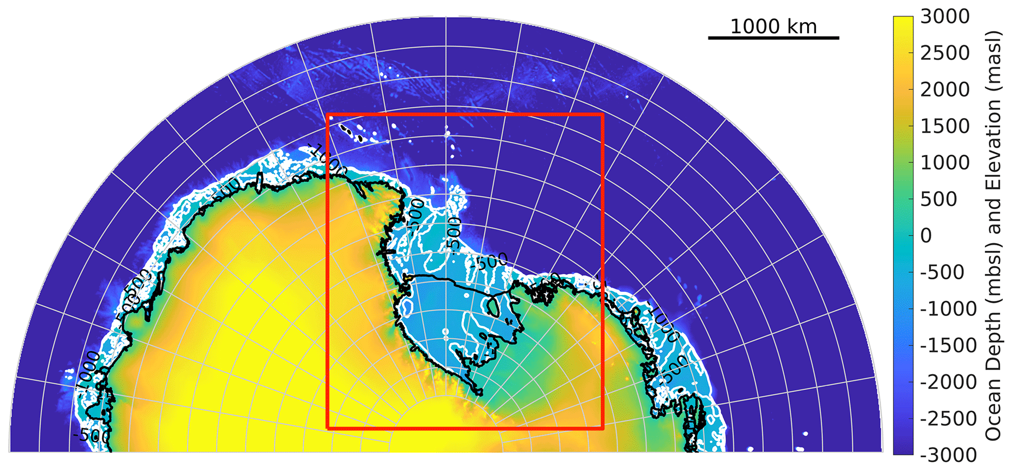
Figure 1Antarctic map with the domain of this study delimited in red. Over open ocean and within ice shelf cavities, colours represent the ocean bathymetry (IBCSO (Arndt et al., 2013)). Over grounded ice sheets, colours represent the surface elevation (topography, Bedmap2). Figure generated with the Antarctic Mapping Toolbox (Greene et al., 2017).
2.2 The atmosphere model: PWRF
The Weather Research and Forecasting model (WRF; Skamarok et al., 2019) is the atmospheric component of the coupled model. It is a non-hydrostatic mesoscale atmospheric model developed by the NCAR (National Center for Atmospheric Research) for both atmospheric research and operational forecasting applications. In this study, we use the Polar-optimised version (PWRF) of the Advanced Research WRF dynamic version 4.1.3 (https://www2.mmm.ucar.edu/wrf/users/download/get_source.html, last access: December 2020). This optimisation has been used to specifically represent the polar climate of the Arctic and Antarctic (Bromwich et al., 2013; Hines and Bromwich, 2008). It enables the sea ice mask to be updated during the simulation and the associated sea ice thickness and snow on sea ice values to be specified using an external field. The land component of PWRF is the community Noah land surface model with multi-parameterisation options (Noah-MP; Niu et al., 2011) and distinguishes between bare ground, land ice (glaciers), and sea ice. The latest version includes a three-layer snow model (Yang and Niu, 2003) and has been shown to perform well against observations at Col de Porte (French Alps) and Sleeper River Watershed (Vermont, USA) (Niu et al., 2011): it improves the representation of surface fluxes, surface meltwater production, percolation, and retention/refreezing in the snow layers and surface runoff and has a refined snow water equivalent reproduction (closer to reality) with an improved diurnal cycle of the snow skin temperature. In this study, PWRF is used over the model domain at approximately 10 km horizontal resolution on a polar stereographic grid. It has 210 × 240 grid cells and 61 vertical levels. The static input data come from the Reference Elevation Model of Antarctica (REMA; Howat et al., 2019) for the land topography and the land use product AntarcticaLC2000 (Hui et al., 2017), processed to be ingested by the WRF model by Gerber and Lehning (2020). The boundary conditions are updated every 6 h using the ERA5 reanalysis (Hersbach et al., 2020). The physics options are the WRF single-moment 5-class microphysics scheme, the latest RRTMG option for both long- and shortwave radiation schemes (Iacono et al., 2008), the conjunction of the Janjic Eta Monin–Obukhov surface layer scheme, and the Mellor–Yamada–Janjic boundary layer scheme (Janjic, 2002), and the setup uses spectral nudging above the 20th model layer for the u and v component of the wind, temperature, and geopotential. The preprocessing of the WRF input files followed the standard procedure (ungrib.exe – metgrid.exe – real.exe, Wang et al., 2019), but once the initialisation step is performed, the input files are altered to match the coastline from MITgcm, and the sea surface temperature and sea ice mask are updated to match those of MITgcm.
2.3 Model domain
We base our coupled model on the SKRIPS model, described in Cerovečki et al. (2022) for the Southern Ocean. This model couples the MITgcm ocean component to the PWRF atmosphere part using the Earth System Modeling Framework (ESMF; Hill et al., 2004) according to the National United Operational Prediction Capability (NUOPC; Sitz et al., 2017) protocols and is available at https://library.ucsd.edu/dc/collection/bb1847661c and https://zenodo.org/record/7336070#.Y_LLqhxBz0o (last access: March 2022). The study domain (Fig. 1) extends from Victoria Land and Cape Adare (160∘ E) to Mary Byrd Land (140∘ W) along the coastline and from 64∘ S, encompassing the Ross Sea, to 88∘ S, including the whole Ross Ice Shelf and the Transantarctic Mountains. This domain has been designed to retain enough of the continent to allow katabatic winds and mesocyclones to develop (Carrasco and Bromwich, 1993; Carrasco et al., 2003) . The same polar stereographic 10 km grid is used for both models, allowing direct transfer of information between the oceanic and atmospheric components (and vice versa) without the need of an additional step of regridding (although ESMF allows for multiple regridding options). Figure 2 illustrates the workflow.
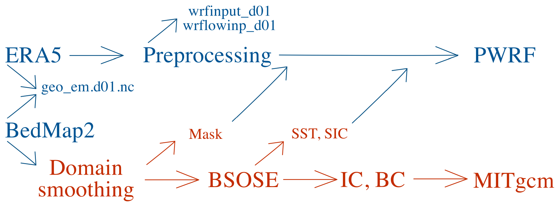
Figure 2Workflow chart of the preprocessing and setting up of the experiments. geo_em.d01.nc, wrfinput_d01, and wrflowinp_d01 are the intermediate files generated by the PWRF preprocessing; IC and BC indicate initial conditions and boundary conditions, respectively.
2.4 Experiments
We run the coupled model in concurrent mode, with a 20 s time step for the atmosphere component and a 1 min time step for the ocean component. We perform two sets of simulations: one set for the summer month of January 2016 and one set for the winter month of August 2016. The experiments were set up with the aim of comparing various model configurations for different sea ice cover conditions (winter vs summer). There are two experiments for each of the sets, (1) the SKRIPS model reflecting the published setup of Cerovečki et al. (2022) and (2) our case study including the conservation of heat and mass, the Polar-SKRIPS model version 1 (P-SKRIPS hereafter, Table 1). The code and experiments for this paper can be found at https://doi.org/10.5281/zenodo.7297744 (Malyarenko and Gossart, 2023a, b). Each of the simulations (1 and 2) is performed first over the whole month with a 10 min coupling time step to evaluate performance and secondly over only an hour with a 1 min exchange time step and 1 min output frequency to directly compare the exchanged variables at specific time steps. For each of the runs, we initialise MITgcm sea ice concentration, sea ice thickness, and snow on ice thickness from the B-SOSE dataset, which then evolves freely within the MITgcm model (except for the snow on sea ice). The updated sea ice concentration mask is then passed on to PWRF.
Table 1Import of heat and mass fluxes versus calculations in the two experiments.
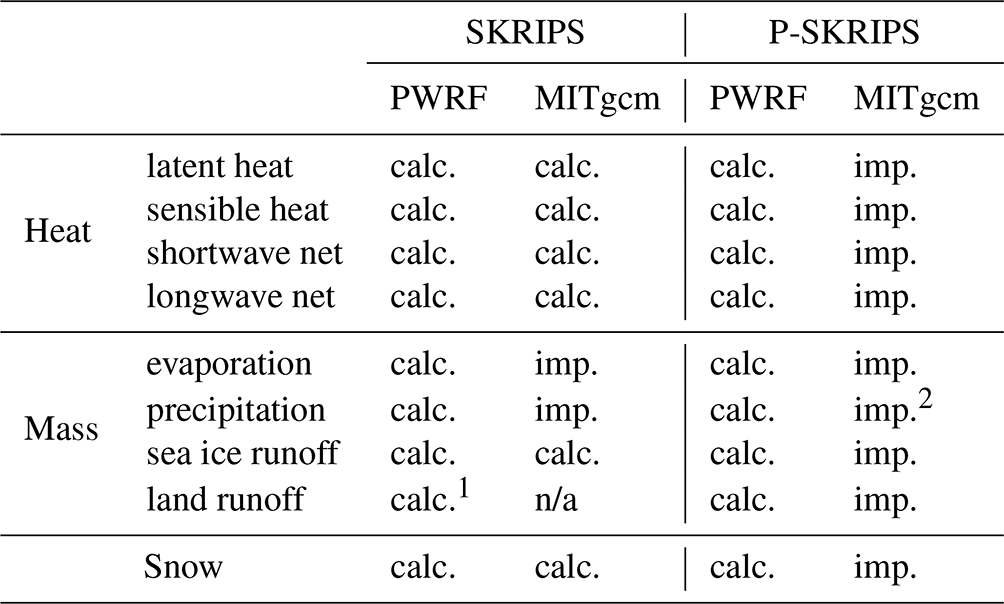
calc.: calculated by the model. imp.: imported from PWRF to MITgcm. 1 calculated but is not accounted for (disappears). 2 no snow deposition in sea ice growth routine. n/a: not applicable.
2.4.1 SKRIPS case
The SKRIPS case reflects the setup for the Southern Ocean by Cerovečki et al. (2022) on which this study is based. Within this framework, the 2 m temperature, specific humidity, 10 m u and v components of wind, and evaporation and precipitation rates, as well as downward longwave and shortwave radiation, are sent from PWRF to the ESMF/NUOPC coupler (Table 1). In MITgcm, all flux components (heat and freshwater mass) and the wind stress are re-calculated using the standard bulk formulae, with the meteorological variables received from PWRF. After the sea ice routine, the net surface heat and mass fluxes are scaled in the mixed cells containing ocean and sea ice in the ocean component. This parallel calculation of fluxes in the models is shown in Fig. 3b and d. The ocean variables are sent to the atmosphere to replace the reanalysis forcing in PWRF: the sea surface temperature, the sea ice concentration and thickness, and the sea surface currents.
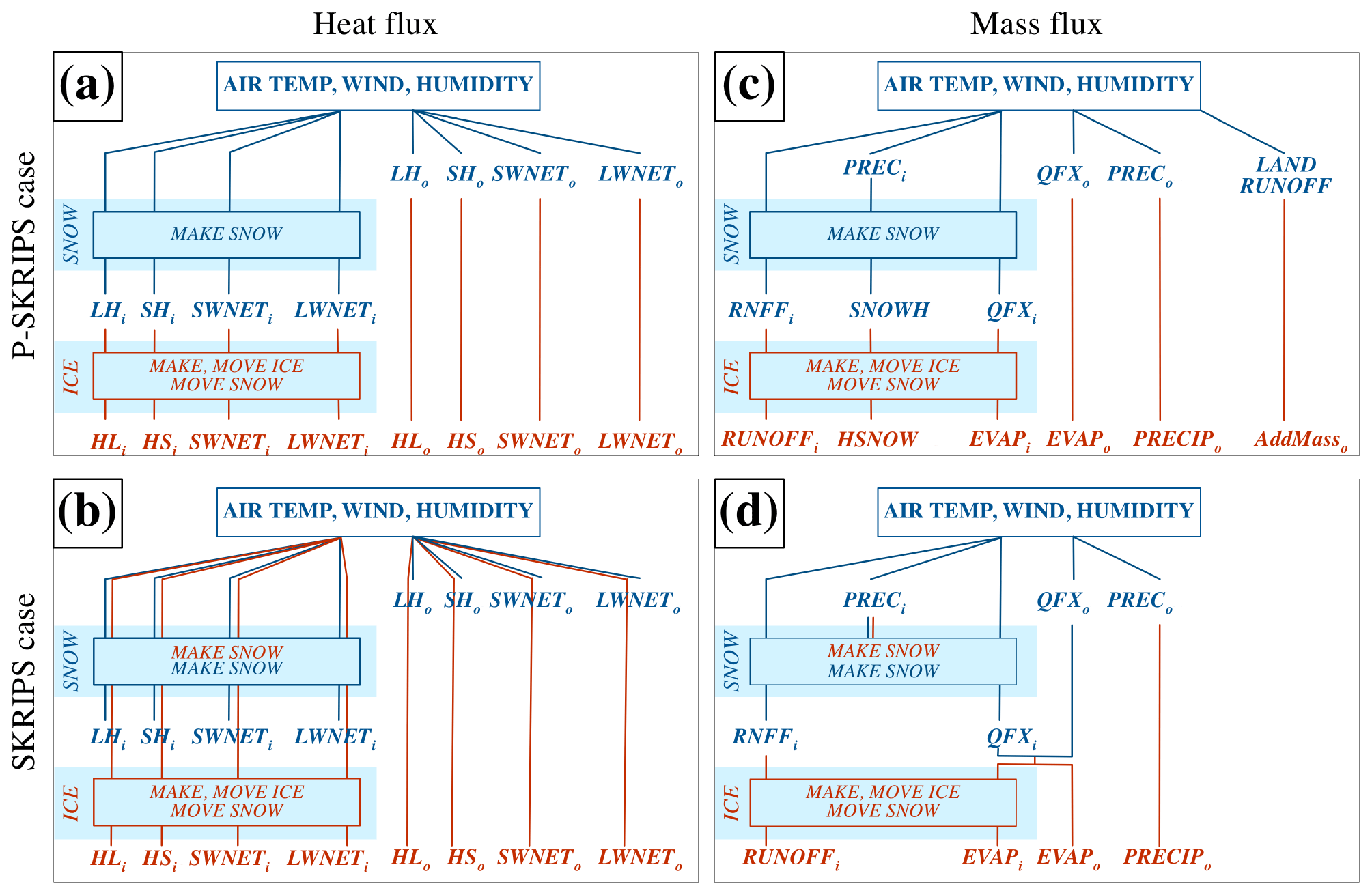
Figure 3Exchanged flux pathways through snow and sea ice routines in PWRF (blue) and MITgcm (red). Panels (a) and (c) represent the P-SKRIPS setup and (b) and (d) the SKRIPS. The i and o indices represent the variable over ice and ocean, respectively. LH, SH, SWNET, and LWNET stand for latent heat, sensible heat, net shortwave radiation, and net longwave radiation (in W m−2). Prec stands for precipitation, QFX and EVAP for surface evaporation and RNFF for surface meltwater runoff (all in mm). SNOWH is the variable for the amount of snow on sea ice (in m). In panels (b) and (d) the overlapping blue and red lines indicate the fluxes are re-calculated by MITgcm and WRF.
2.4.2 P-SKRIPS case
In this study, we attempt to conserve the heat and mass fluxes sent from the atmosphere into the ocean by importing the fluxes computed by PWRF to MITgcm directly, bypassing the recalculation in the oceanic component (Table 1). In the original code, part of the energy flux is changed by the PWRF snow pack calculations prior to sending the field to MITgcm. Because MITgcm also has a snow on sea ice routine, it calculates an additional change on snowpack physics. To avoid this double change, we capture the flux variables after they have gone through the snow on ice physics in PWRF (just after the seaice_noah call in surface_driver.F90) to pass to MITgcm. In addition, the calculation of fluxes (in seaice_solve4temp.F) and calculations of snow growth/melt (in seaice_growth.F) are turned off in MITgcm. PWRF calculates the surface evaporation and runoff resulting from the snow on sea ice melt. These freshwater fluxes are captured and transferred to MITgcm in the same fashion, including turning off the calculations representing these processes (in seaice_growth.F) in MITgcm. Precipitation over sea ice has been converted into sea ice surface snow thickness change by PWRF; we therefore do not account for snowfall deposition in MITgcm. Finally, the land surface runoff is integrated for the whole ice shelf in PWRF and added in MITgcm at the coastline as a freshwater mass flux into the ocean (utilising the AddMass option in MITgcm). The schematic representation of this flow of fluxes is shown in Fig. 3a and c. The coupling interface between the atmosphere and ocean models is defined as (1) air–ocean over open ocean and (2) between the sea ice (changes and advection of sea ice simulated by the ocean model) and the snow layer on top of it (accumulation and compaction are dealt with by the atmosphere model). Since multi-layer snowpacks have been reported as an improvement for snow on sea ice representation (Arduini et al., 2022), the Noah-MP multilayer snowpack is better suited to simulate the snowpack changes and properties in PWRF rather than snow on sea ice physics in MITgcm. The snow compaction/accumulation and thermodynamic changes (and interactions with radiative fluxes) all occur in PWRF, which then sends the snow thickness to MITgcm. The latter updates its snow on sea ice thickness variable accordingly. The ocean model then advects the sea ice (including the snow on top of it), and the new sea ice concentration and thickness are sent back to PWRF.
2.5 Scaling by the sea ice concentration mask
The development of P-SKRIPS includes the import of the individual heat and mass flux components from PWRF into MITgcm. The import of surface fluxes in the external forcing package (exf package) is prohibited when using the sea ice package in a standard version of MITgcm because the fluxes need to be calculated according to the sea ice mask. We have set up the two models with the same grid and the same ice–ocean mask between PWRF and MITgcm, so the fluxes can be directly used in the sea ice packages, without any mask mismatch. We thus remove this error flag from seaice_model.F (in MITgcm). This standard import method (used in SKRIPS) consists in directly importing the PWRF output variable (XPWRF) to MITgcm. When XPWRF refers to any component of the heat flux, latent, sensible, shortwave, and longwave net fluxes or evaporation, it is scaled to account for mixed grid cells, partially occupied by sea ice in the model cell in PWRF (Fig. 4a). This occurs mid-time step (module_surface_driver.F in PWRF), and the PWRF model output contains these scaled variables. The “direct import” variable path in Fig. 4b illustrates how this scaled XPWRF is then imported as is into the MITgcm exf package. This implies that when MITgcm receives the variable and accounts for the presence of sea ice in its own routines, the variables are scaled twice, thereby affecting the amount of heat gained or spent over the sea ice areas. In the P-SKRIPS version, we exchange the four heat flux components between the models for physical consistency. To tackle the double-scaling issue, we have developed a new technique (referred to as “separate fluxes”), illustrated in Fig. 4c, whereby the separate heat flux components are captured in PWRF over the sea ice and over the ocean separately (Xice and Xocean). In this new approach two variables are now imported from PWRF to MITgcm, for each heat flux component: Xocean becomes the exf variable, and Xice is used instead of the recalculation of fluxes (solve4temp.F in MITgcm) to determine the amount of heat available for sea ice growth/melt (F_ia variable). This ensures that the fluxes are calculated and scaled only once between the two models.
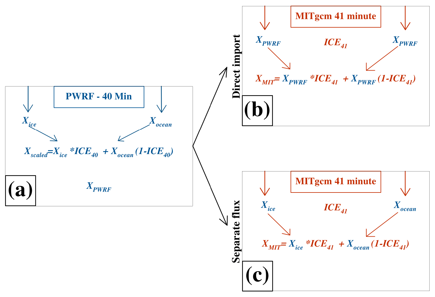
Figure 4Variations in the variables exchange between the models: (a) PWRF variable output and (b) direct import of variable (a) into the MITgcm model, versus (c) separate flux variable exchange. X represents any heat flux component in both models. Xice is the flux value over sea ice, and Xocean is the flux value over the open ocean. Xscaled is calculated mid-time step in PWRF, while XPWRF is available as output at the end of the time step. ICE40 and ICE41 represent the sea ice concentration calculated by MITgcm at the respective time step. XMIT is the heat flux received from PWRF and available for the ocean model after scaling (not calculated for each flux component in MITgcm, only for the total heat flux, but used here to directly compare to XPWRF).
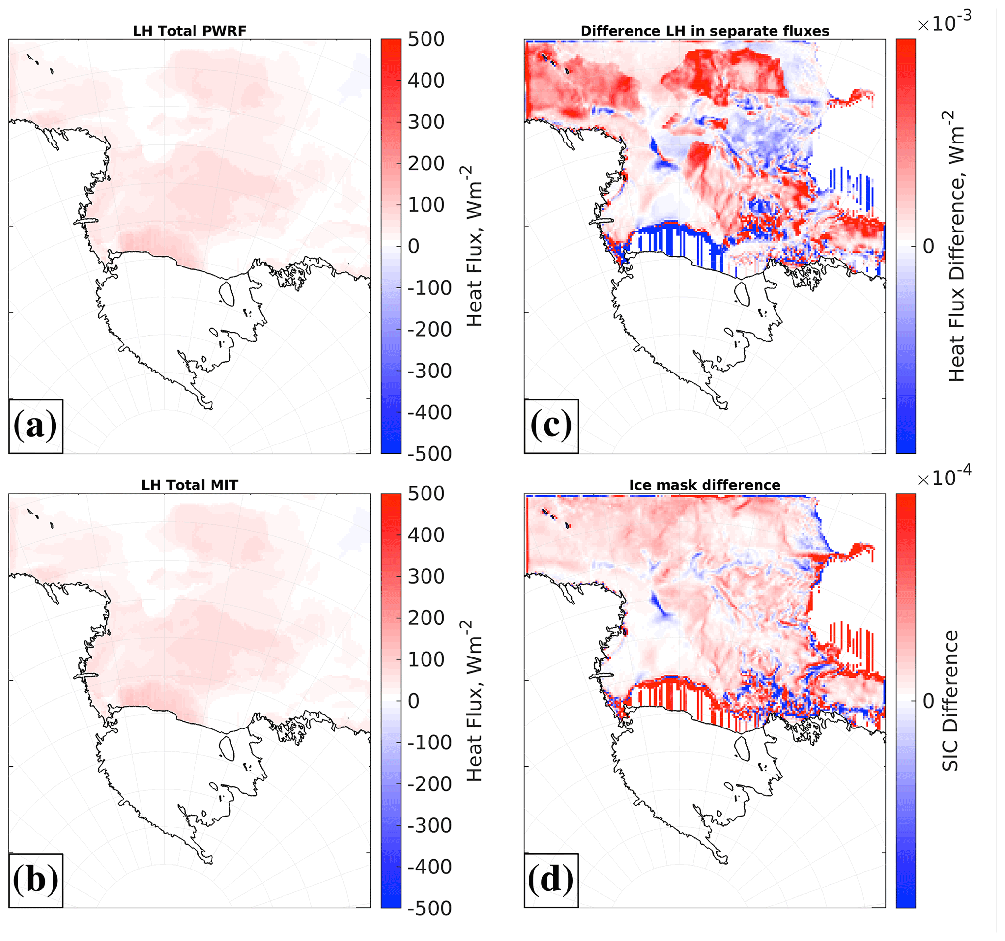
Figure 5(a) Latent heat (LH) flux: total heat flux in PWRF using the capture of the separate fluxes, (b) latent heat in MITgcm, (c) differences between (a) and (b), and (d) ice concentration mask difference between the two time steps. The full range of differences for (c) is −0.08 to 0.02 W m−2. See Sect. 2.5 for more details.
Figure 5 shows an example of this approach for the latent heat flux: (a) XPWRF, (b) XMIT, (c) XPWRF−XMIT, and (d) sea ice concentration difference ICE40 − ICE41. The separate flux approach reduces the differences between the two models to negligible amounts (Fig. 5c). Firstly, the differences between Xscaled and XPWRF (Fig. S2a) are due to the fact that the heat fluxes variables are affected by subsequent processes after the mid-time-step scaling in PWRF, when these variables are captured to be sent to MITgcm. Such processes encompass albedo changes affecting the upwelling shortwave, the skin surface temperature and the upwelling longwave radiation, but these are trivial compared to the range of the exchanged fluxes. Due to the nature of the coupling, the sea ice concentration mask evolves between minutes 40 and 41 (Fig. 5d). Thus, the values of XPWRF correspond to the flux using the sea ice concentration sent from MITgcm at 40 min. PWRF sends XPWRF to MITgcm to be used for time step 41, using the sea ice concentration mask at that time step. Hence even in the separate flux approach, Xscaled and XMIT are not exactly the same. Because the ice concentration mask difference is small, the scaling multiplication by XICE, which is ∼104 (Fig. 5d), results in subtle differences in the order of 10−3 W m−2. The sign definition of each of the flux components is listed in Table S1. We note that additional heat is spent on sea ice thermodynamics by MITgcm (in seaice_growth.F), so the resulting sum of fluxes available to the ocean model (Qnet) is not the same as a sum of the four heat flux components (XMIT). This is why we created extra diagnostic variables.
We now present results of the different experiments, looking first at the conservation of heat fluxes. We look into the conservation of mass, and we introduce the land runoff variable that describes the melting of snowpack on the ice sheet and its flow into the ocean. Lastly, we compare the results of the different model setups over a month-long simulation.
3.1 Conservation of heat
3.1.1 Import of the heat flux in the P-SKRIPS model
Figure 6 shows each of the fluxes exchanged or calculated in PWRF at 40 min and MITgcm at 41 min (from the high frequency exchange simulation, the time step was chosen close to the start of the simulation). The 1 min offset represents the fact that the fluxes are calculated in PWRF at 40 min (first column in Fig. 6) and then imported into MITgcm at the 41st min. In the P-SKRIPS setup (second column in Fig. 6), MITgcm directly receives the fluxes calculated in PWRF at the preceding time step, while in the SKRIPS case, MITgcm at 41 min uses PWRF 40 min output to recalculate the fluxes (third column in Fig. 6). In order to differentiate the fluxes over sea ice from over the ocean surface, we implement additional diagnostic variables in MITgcm (in seaice_solve4temp.F). The second and third columns in Fig. 6 merge the MITgcm sea ice and ocean components of each of the heat flux variables to ensure that we compare the same variables as in PWRF output. The comparison of the first column (PWRF) and the second column (MITgcm in P-SKRIPS) indicates that the fluxes were successfully imported from PWRF to MITgcm. While the P-SKRIPS and the SKRIPS cases (columns 2 and 3) show similar flux distributions and magnitude of fluxes, there are visible differences between the two. The differences are not clearly attributable to any single variable, as all of the surface atmosphere and sea ice state parameters are included in the flux calculations. The sea ice mask, the state of snow on ice (thickness, wetness, albedo), the calculation of surface temperature, and surface friction velocity in bulk formulas create a mosaic of differences between the heat flux maps. In January, the flux distribution differences are related to the presence or absence of sea ice. We attribute those differences to the calculation of fluxes in the sea ice package in MITgcm (maps in the last column of Fig. 6). In contrast, most of the domain is covered by sea ice in August. At that time, longwave and shortwave net heat fluxes show more homogenous differences, reflecting only different emissivity coefficients and albedo values. The turbulent heat fluxes are shown to be connected to the extra moisture brought by a precipitation event (Fig. S1). In general, the differences between the two cases reflect inconsistencies in the calculations between the two models: (1) there are differences in the momentum calculations used in bulk formulae for the latent and sensible heat components calculation and the evaporation over snow and ice calculation; (2) small distinctions arise due to slightly different emissivity coefficients used in the calculation of the upward longwave radiation; (3) the differences in the upward shortwave radiation are a result of conflicting albedo calculations between the two models, based on differing assumptions of dry/wet snow and snow threshold; and (4) the sea ice mask varies between the two cases, and PWRF internal heat flux calculations assess the presence of sea ice based on a predetermined threshold. By directly importing the heat fluxes from the atmosphere to the ocean and vice versa, we avoid the differences induced by the parallel calculations of fluxes in the two components that would lead to inconsistencies between the flux in the two coupled models. We thus highly recommend the import of fluxes in each model component in order to conserve the fluxes for the general balance of the coupled model.
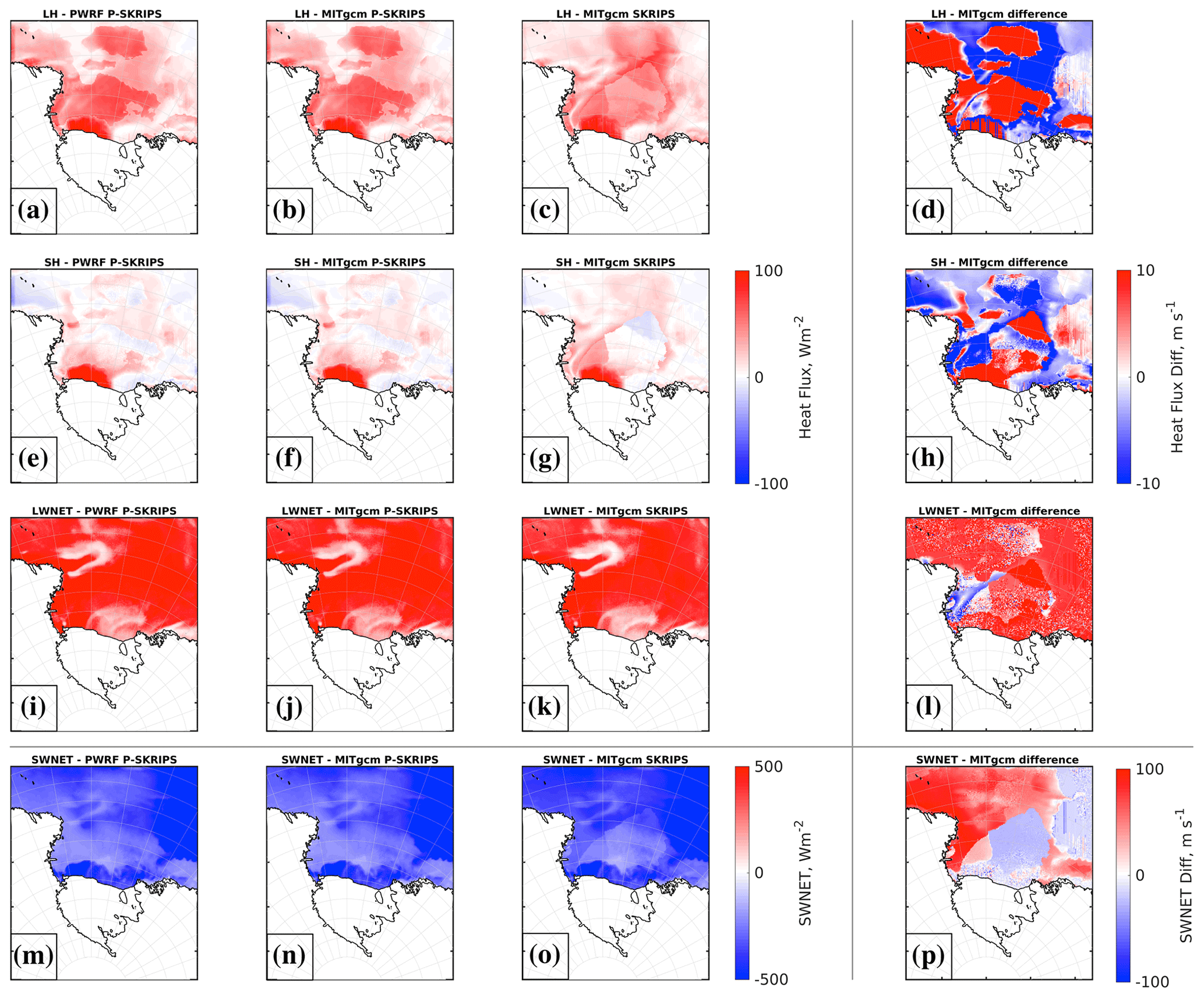
Figure 6Maps of fluxes calculated or imported between models (PWRF, first column; MITgcm in the P-SKRIPS model, second column; MITgcm in the SKRIPS case, third column; and difference between the MITgcm in P-SKRIPS and in SKRIPS, fourth column). See Sect. 3.1.1 for model details. Plots for the January experiment; see August experiment in the Fig. S1. Positive heat flux is defined upward.
3.2 Conservation of mass in the P-SKRIPS model
3.2.1 Precipitation, evaporation, and runoff
To avoid repeated accumulation of snowfall over sea ice in each model component, the deposition of snow is neglected in MITgcm (seaice_growth). The new mass of snow is accounted for by the exchange of the height of the snow on sea ice variable (SNOWH) sent by PWRF to MITgcm after the deposition, compaction, and metamorphism of the snow cover have taken place in the atmospheric component. The snow falling over the open ocean, however, is taken care of by MITgcm. The evaporation at the snow/ice surface due to interactions with the atmosphere is another process that is accounted for in both PWRF and MITgcm. Analogous to the heat fluxes, in the coupled model, the snowpack module of PWRF generates the evaporation flux that is directly imported by MITgcm (in seaice_growth). In addition, this time the scaling to resolve mixed ocean–sea ice cells is ignored in MITgcm (in seaice_growth) as it was already applied in PWRF. Figure 7 shows a similar range and pattern for the two simulations, where the variations occur for regions of differing sea ice concentration mask. Finally, the melt occurring at the surface of the snow and not retained in the snowpack (by refreezing) is exported in the form of runoff in PWRF (SFCRUNOFF). In MITgcm, the input of freshwater from runoff usually comes from river runoff but is used here to collect the water melted from the snow layer present over the sea ice. This variable is directly imported from PWRF and is captured in the atmosphere component by adding an option to store the variable over sea ice (in addition to the land-only variable). This evolution is also noticeable in Fig. 7 as the differences between columns 2 and 3 reflect the varying amounts of surface meltwater calculated by each of the models independently (SKRIPS case) or directly imported into MITgcm from PWRF (P-SKRIPS case).
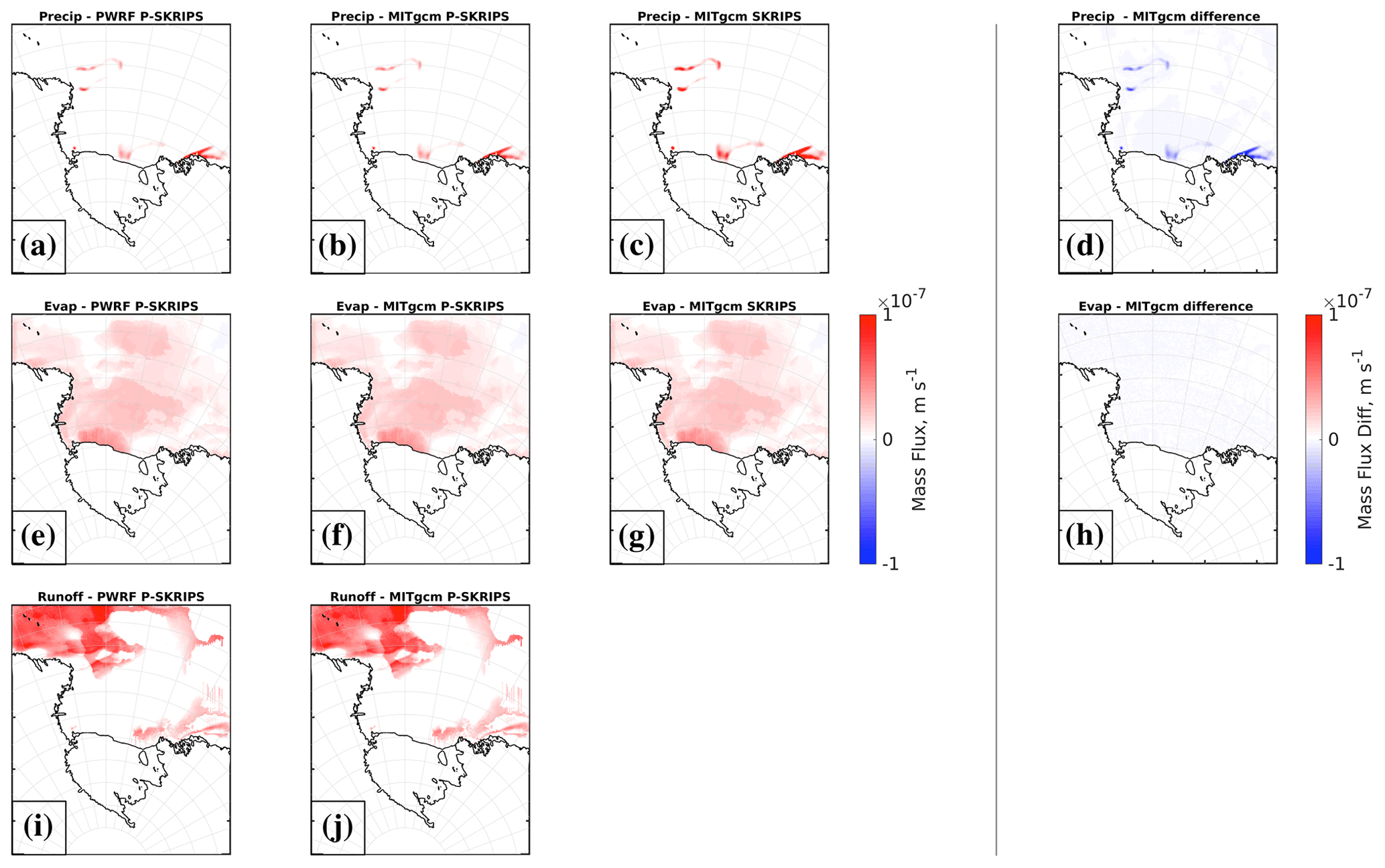
Figure 7Maps of fluxes calculated or imported between models (PWRF, first column; MITgcm in the P-SKRIPS model, second column; MITgcm in the SKRIPS case, third column; and difference between the MITgcm in P-SKRIPS and in SKRIPS, fourth column). See Sect. 3.1.1 for model details. Plots for the January experiment; see August experiment in the Fig. S3. Positive evaporation is defined upward, and positive precipitation and runoff are defined downward.
3.2.2 Ice sheet runoff
In addition to the meltwater runoff over sea ice, PWRF generates another surface mass balance term over land: runoff from the surface of the ice sheet that needs to be redirected to the ocean. In the standalone simulations of PWRF, the meltwater that does not refreeze into the snowpack and runs off is treated as a sink term and does not affect any other component. In the coupled framework, we identify the ice sheet meltwater runoff as an important component of the total mass budget that has an effect on any future projections (Golledge et al., 2019). For that reason, we capture the land ice meltwater runoff and send it to MITgcm. Because the land surface runoff is a cumulative variable, only the change in surface runoff (i.e. the amount from that coupling time step minus the amount from the previous coupling time step) is passed to the coupler and to MITgcm. The land surface runoff is integrated along the y axis (meridional integration) within the ESMF-MITgcm interface (get_field_parameters.F90; a new variable, land_runoff, is added as a part of the exf package). We use the MITgcm AddMass variable to add this meltwater into the ocean component. First, we create a mask variable (AddMassInit), read from an external file and fixed in time. It is used to mask the integrated land_runoff from the atmosphere component. This creates a variable AddMass null everywhere, except along the front of the Ross Ice Shelf, where it has the integrated value of the land surface runoff to be added to the ocean as freshwater. However, this approach creates issues. First, the meltwater is not collected from the whole of the ice sheet within the domain but only from cells at the same x-axis value as our mask identifies, which is along the coast of the ice shelf in an east–west direction. Thus, we are missing meltwater runoff from the Drygalski Ice Tongue, from other small ice shelves, and from the eastern and western edges of the Ross Ice Shelf that are not aligned with the ice shelf front (not at the same x-axis value in the grid). Second, we assume no lag for the runoff getting into the ocean, implying that the meltwater runoff originating at the southernmost part of the domain is added to the ocean within one coupling time step (1 min), not accounting for delay in the time it takes the meltwater to arrive to the ice shelf front. This will be addressed in the future developments. The code has been tested with a test value in the coupler (not shown), but the January and August 2016 simulations do not generate any meltwater runoff over the ice sheet due to the limited simulation time, meaning that the import of the variable gives a net zero flux. This new surface mass balance variable is nevertheless added to the coupled model in order to close the mass balance in future work.
3.3 Flux differences during a 1-month experiment
Figure 8 displays the January 2016 time series for each of the integrated fluxes presented in Figs. 6 and 7. We integrate all flux components over the ocean (we ignore land) and present the fluxes at the atmosphere–ocean or snow–sea ice interface, following Fig. 6 (through the coupling interface). The PWRF–P-SKRIPS and MITgcm–P-SKRIPS curves overlap closely for each of the variables. We have significantly reduced the differences between PWRF and MITgcm fluxes in the original SKRIPS setup and in our P-SKRIPS model (Fig. 9 for the January case and Fig. S5 for the August case). There are small differences in the PWRF flux variables between the P-SKRIPS and the SKRIPS cases, expressed either as larger minima (in the case of shortwave fluxes) or as divergence over time. This is because the simulations show different responses to the conservation of fluxes versus parallel calculation (see also Figs. 9 and S5). In summer, the incoming shortwave radiation is at its maximum in the middle of the day, and the differences in albedo parameterisation between PWRF and MITgcm account for the variations in the magnitude of the shortwave peak.
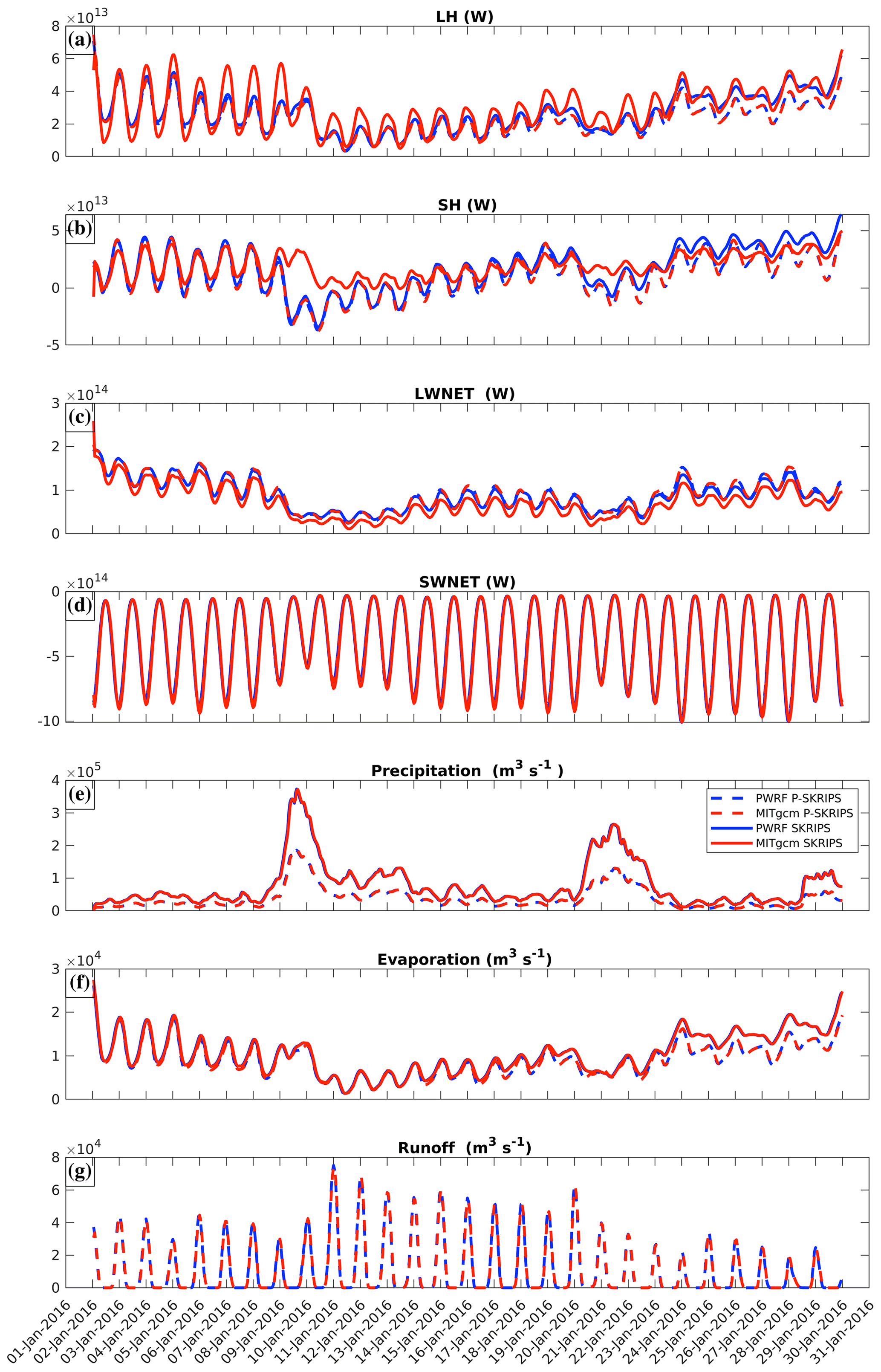
Figure 8Integrated flux time series through the coupling interface for the January 2016 experiment. The P-SKRIPS case is dashed, and the SKRIPS case is shown by solid lines. PWRF fluxes are in blue, and MITgcm are in red. Heat fluxes are defined positive upwards, the evaporation is defined positive upwards, and the precipitation and runoff are defined positive downwards. For more details, see Sect. 3.3. For the August experiment results, see Fig. S4.
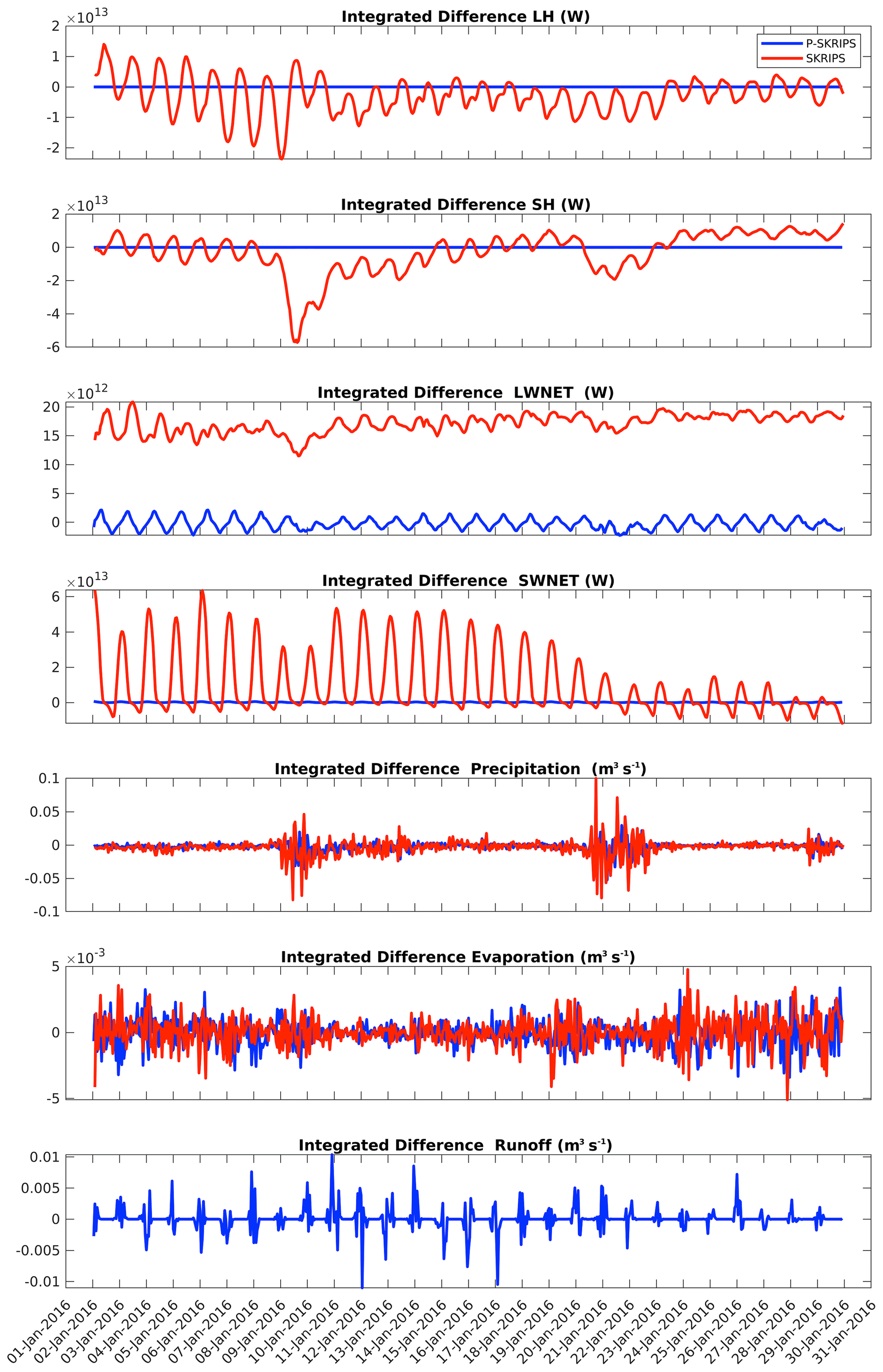
Figure 9Differences of the integrated flux time series through the coupling interface for the January 2016 experiment. The P-SKRIPS case is displayed in blue, and the SKRIPS case is in red. Heat fluxes are defined positive upwards, the evaporation is defined positive upwards, and the precipitation and runoff are defined positive downwards. For more details, see Sect. 3.3. For the August experiment results, see Fig. S5.
The largest discrepancies in heat fluxes are between the MITgcm results from the direct import method used in P-SKRIPS case and the independent calculation used in the SKRIPS case. In summer, differences in the shortwave net calculations between PWRF and MITgcm in the SKRIPS case dominate the heat flux inconsistencies (on average, an order of magnitude larger than the turbulent heat fluxes differences, Table S2). In August, when the sun is low on the horizon, the sensible heat and longwave radiation fluxes show the largest differences between PWRF and MITgcm (Fig. S4). The ocean receives a larger amount of latent heat in the SKRIPS simulation with an almost constant bias of 1.1013 W. The differences in sensible heat flux into the ocean vary over time between the two models. Larger discrepancies are associated with precipitation events (6–8 August, 12 August, 14–19 August, and 26–31 August, except 29 August), leading to a loss of heat from the ocean for the SKRIPS simulation, while the P-SKRIPS simulation indicates a gain for the ocean. The longwave net radiation in the SKRIPS case is always slightly underestimated, as compared to the P-SKRIPS, although both curves show very similar variations over time. Despite the fact that precipitation is directly imported from PWRF to MITgcm (also in the SKRIPS case), the amount of precipitation sent by PWRF to MITgcm is overestimated. This is because in the SKRIPS case the total precipitation is made out of the sum of the time step non-convective precipitation (RAINNCV) and non-convective snow and ice (SNOWNCV). However, the latter is defined as a component of the non-convective precipitation, which encompasses all species (rain, graupel, and snow and ice) and, therefore, is accounted for twice in the precipitation term. It is likely that over the course of the winter season, additional accumulation of snow over the sea ice affects the heat transfer through that layer, and in spring it will lead to increased freshwater flux into the surface of the ocean. In the P-SKRIPS, the components are added individually, and the non-convective precipitation term is ignored. As evaporation is directly imported from PWRF to MITgcm in both cases, no large difference exists between the two simulations. In the last week of the simulation, the fluxes in the two experiments diverge more and more, due to the (now correct) balancing of the fluxes. Finally, the runoff over sea ice is an additional modification in the P-SKRIPS that does not exist in the SKRIPS case. Therefore, only the PWRF and MITgcm balanced outputs are present and match almost perfectly (see Tables S3 and S4 for more information).
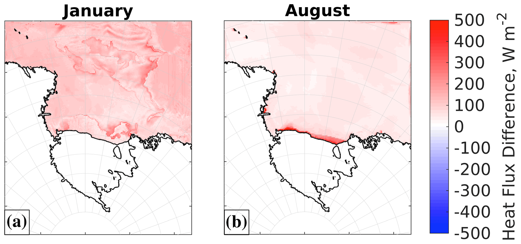
Figure 10Maximum differences of total heat flux exchanged for the January and August 2016 experiments.
The differences in heat flux calculation between PWRF and MITgcm have a clear spatial distribution, and the highest discrepancies are linked to areas of open water along the coast in August (ocean polynyas). Differences in the Fig. 10 and in the text hereafter are defined as PWRF-MITgcm, with heat fluxes defined as positive upward. Due to the strong winds keeping the polynyas open, the turbulent heat fluxes differ significantly in the SKRIPS simulation: maximum differences are 922 W m−2 for sensible heat flux and 318 W m−2 for latent heat flux (PWRF producing larger values). The total heat flux difference ranges from −295 to 1212 W m−2 in August. In January, the difference of the total heat flux is smaller (−466 to 392 W m−2) and is comparable with the shortwave heat flux difference alone (−455 to 424 W m−2). Maximum absolute differences are located at the edge of the sea ice, where snow on ice calculation is most important for the total heat flux. These reflect the imbalance of heat flux calculations in coupled models, now corrected in the P-SKRIPS model. It highlights the importance of conservation of heat and mass fluxes, especially when polynyas are considered.
In this paper we have conserved water and energy fluxes between the ocean and atmosphere components of the P-SKRIPS coupled model setup for the Ross Sea domain. We have provided a detailed analysis of flux pathways in each of the components of the coupled model and described strategies for the conservation of the variables exchanged. One-month test experiments for the January and August of 2016 have been carried out and show that the P-SKRIPS approach homogenises the ocean and atmosphere calculations. This is an improvement to pre-existing ocean–atmosphere coupling in regional climate models and is needed for balanced long-term simulations, especially in coastal polynyas.
P-SKRIPS also splits the processes related to sea ice between the two models. The formation and advection of sea ice stay in MITgcm. The snow cover changes were happening in both PWRF and MITgcm in the previous version of the model, leading to inconsistent snow on sea ice. In P-SKRIPS, the snow cover changes only happen in PWRF and are then sent to MITgcm. Its multi-layered snowpack and complex representation of snow on sea ice makes PWRF more suitable to represent the snow/ice–atmosphere interactions. As stated in Arduini et al. (2022), firstly, by its insulating effect, reducing the heat exchange from the ocean through the sea ice and snow on sea ice to the atmosphere, the representation of strong cooling events and surface-based inversions is enabled. Secondly, by having better (several layers of snow) schemes, changes in the atmosphere are better captured and the snow responds quicker to those changes. Thirdly, the ratio of snow on sea ice and sea ice thickness is thought to be almost constant in Antarctica (Jeffries et al., 1998; Toyota et al., 2011; Worby et al., 1996), which implies that changes in thickness of the snow on sea ice impact the sea ice thickness (Toyota et al., 2016). In addition, the snow on sea ice initialisation depends on a couple of settings in the atmospheric component and prescribing too thin a snow cover (0.0005 m, seaice_albedo_opt = 1 in PWRF namelist.input) leads to a unrealistically large negative latent heat flux over sea ice (400 W m−2). Hopefully, more detailed and accurate observations of the snow on sea ice cover will be available in the future, to help the initialisation of this parameter in the models and to enable their validation. We identify a series of potential improvements to P-SKRIPS that are listed below and will be the focus of future research:
-
In summer, large differences in shortwave fluxes are directly linked to the calculation of the albedo, which varies between the model components as they have different parameterisations of dry/wet snow. We believe that exchanging the snow on sea ice albedo value between the models, as suggested by Ren et al. (2021), would be an improvement, but it requires a series of alterations in the sea ice routine in PWRF (module_sf_noah_seaice.F90) to facilitate the use of the albedo variable.
-
The two-way exchange of snow on sea ice variables between the atmosphere and the ocean models would allow the snow cover thermodynamic changes to take place in PWRF. This would send the snow on sea ice thickness information to MITgcm that could then advect and flood the snow on top of sea ice as the ocean moves it around. At the moment, the snow on sea ice thickness information is passed from PWRF to MITgcm and moved around by the ocean component but not sent back to PWRF.
-
Sending back the snow on sea ice variable to PWRF once it has been advected in MITgcm is an important future development. Currently, PWRF does not have the ability to remove the snow on ice once the sea ice has been advected: if a sea ice cell moves and is replaced by an open ocean cell, the snow on sea ice layer will remain present in the now ocean cell. The snowpack calculations occur only for sea ice-filled cells; thus PWRF ignores the snow on sea ice values for now open ocean cells. The “old” snow on ice will be used in case of new sea ice advection or growth at this location, for example, within the polynyas where sea ice is constantly moving. This should be addressed in the future in order to get rid of the relict of the snow on sea ice layer over ocean cells.
-
The momentum variables have not been balanced in this version of the coupled model: the wind stress is calculated and accounted for in MITgcm, using the u and v wind components passed on from the atmosphere.
-
Bulk fluxes calculated by the ocean and atmosphere are quite different. The sea ice package in MITgcm was created for and tuned according to the ocean model. It needs further refinements to work smoothly with the directly imported fluxes from PWRF. In short, in the balanced coupled model, MITgcm needs tuning to the new atmospheric forcing.
The development of the coupled Polar Scripps-KAUST PWRF-MITgcm model presented in this paper makes conservation of heat and mass possible over long-term simulations, which is necessary for more reliable future projections. The energy imbalance of up to 922 W m−2 due to non-conservation of energy in the previous Scripps-KAUST version of the model likely affects the heat content of the atmosphere and deep convection of the ocean. While the atmosphere's response to the extra energy is the formation of localised weather events, the ocean's response to a reduced amount of heat flux leads to a weakening of the formation of the Antarctic Bottom Water in polynyas in the Ross Sea. The presented coupled model setup constitutes, to our knowledge, the most physically consistent representation of ocean–atmosphere–sea ice interactions for polar climates and is thus recommended for climate modelling in any Arctic and Antarctic region.
Our model code for the Ross Sea case is based on PolarWRF and MITgcm. The P-SKRIPS model code is an updated version of SKRIPS (https://doi.org/10.5281/zenodo.7336070, Sun, 2022) and can be found in the two directories due to size limits (https://doi.org/10.5281/zenodo.7739063, Malyarenko and Gossart, 2023a and https://doi.org/10.5281/zenodo.7739059, Malyarenko and Gossart, 2023b). The detailed instructions for converting WRF to PWRF (https://doi.org/10.1029/2012JD018139, Bromwich et al., 2013) can be found within the PSKRIPS main folder. The short description of steps for PWRF is as follows: find PSKRIPS/Models/WRF_4.1.3 within the repository, obtain PWRF-4.1.3 modifications by email and merge the code locally, add P-SKRIPS modifications to PWRF, and compile. ERA5 Reanalysis data (0.25∘ Latitude-Longitude Grid), generated by the European Centre for Medium-Range Weather Forecasts, are available at https://doi.org/10.24381/cds.bd0915c6 (Hersbach et al., 2023a) and https://doi.org/10.24381/cds.adbb2d47 (Hersbach et al., 2023b). BSOSE data are available at http://sose.ucsd.edu/SO6/ITER135/ (Mazloff et al., 2010). The Bedmap 2 data can be downloaded from https://www.bas.ac.uk/data/our-data/maps/thematic-maps/bedmap2/, (Fretwell et al., 2013).
The supplement related to this article is available online at: https://doi.org/10.5194/gmd-16-3355-2023-supplement.
AM and AG designed the study and developed the P-SKRIPS version of the model. MK and RS helped with the technical implementation of the model developments. Visualisation and analysis of results were carried out by AM and AG. All authors contributed to writing and editing the manuscript.
The contact author has declared that none of the authors has any competing interests.
Publisher’s note: Copernicus Publications remains neutral with regard to jurisdictional claims in published maps and institutional affiliations.
The modelling has been supported by the New Zealand e-Science Infrastructure (NeSI). Alena Malyarenko and Alexandra Gossart would like to thank Alexander Pletzer, Chris Scott, Wes Harrell, and Aleksandr Beliaev for technical help.
This research has been supported by the Ministry of Business, Innovation and Employment (grant no. ANTA 1801).
This paper was edited by Christopher Horvat and reviewed by Guillaume Boutin and one anonymous referee.
Agosta, C., Fettweis, X., and Datta, R.: Evaluation of the CMIP5 models in the aim of regional modelling of the Antarctic surface mass balance, The Cryosphere, 9, 2311–2321, https://doi.org/10.5194/tc-9-2311-2015, 2015. a
Agosta, C., Amory, C., Kittel, C., Orsi, A., Favier, V., Gallée, H., van den Broeke, M. R., Lenaerts, J. T. M., van Wessem, J. M., van de Berg, W. J., and Fettweis, X.: Estimation of the Antarctic surface mass balance using the regional climate model MAR (1979–2015) and identification of dominant processes, The Cryosphere, 13, 281–296, https://doi.org/10.5194/tc-13-281-2019, 2019. a, b
Alam, A. and Curry, J.: Lead-induced atmospheric circulations, J. Geophys. Res.-Oceans, 100, 4643–4651, https://doi.org/10.1029/94JC02562, 1995. a
Arduini, G., Keeley, S., Day, J., Sandu, I., Zampieri, L., and Balsamo, G.: On the importance of representing snow over sea-ice for simulating the Arctic boundary layer, J. Adv. Model. Earth Syst., 14, e2021MS00277, https://doi.org/10.1029/2021MS002777, 2022. a, b
Arndt, J., Schenke, H., Jakobsson, M., Nitsche, F., Buys, G., Goleby, B., Rebesco, M., Bohoyo, F., Hong, J. andBlack, J., Greku, R., Udintsev, G., Barrios, F., Reynoso-Peralta, W., Taisei, M., and Wigley, R.: The International Bathymetric Chart of the Southern Ocean (IBCSO) Version 1.0 – A new bathymetric compilation covering circum-Antarctic waters, Geophys. Res. Lett., 40, 3111–3117, https://doi.org/10.1002/grl.50413, 2013. a
Azaneu, M., Kerr, R., and Mata, M. M.: Assessment of the representation of Antarctic Bottom Water properties in the ECCO2 reanalysis, Ocean Sci., 10, 923–946, https://doi.org/10.5194/os-10-923-2014, 2014. a
Banwell, A., MacAyeal, D., and Sergienko, O.: Breakup of the Larsen B Ice Shelf triggered by chain reaction drainage of supraglacial lakes, Geophys. Res. Lett., 40, 5872–5876, https://doi.org/10.1002/2013GL057694, 2013. a
Beadling, R., Russell, J., Stouffer, R., Mazloff, N., Talley, L., Goodman, P., Sallee, J., Hewitt, H., Hyder, P., and Pandde, A.: Representation of Southern Ocean Properties across Coupled Model Intercomparison Project Generations: CMIP3 to CMIP6, J. Climate, 33, 6555–6581, https://doi.org/10.1175/JCLI-D-19-0970.1, 2020. a
Bell, R., Banwell, A., Trusel, L., and Kingslake, J.: Antarctic surface hydrology and impacts on ice-sheet mass balance, Nat. Clim. Change, 8, 1044–1052, https://doi.org/10.1038/s41558-018-0326-3, 2018. a
Bozkurt, D., Bromwich, D., Carrasco, J., and Ronadnelli, R.: Temperature and precipitation projections for the Antarctic Peninsula over the next two decades: contrasting global and regional climate model simulations, Clim. Dynam., 56, 3853–3874, https://doi.org/10.1007/s00382-021-05667-2, 2021. a, b
Bromwich, D.: Snowfall in High Southern Latitudes, Rev. Geophys., 26, 149–168, https://doi.org/10.1029/RG026i001p00149, 1988. a
Bromwich, D., Otieno, F., Hines, K., Manning, K., and Sihlo, E.: Comprehensive evaluation of polar weather research and forecasting model performance in the Antarctic, J. Geophys. Res.-Atmos., 118, 274–292, https://doi.org/10.1029/2012JD018139, 2013. a, b, c
Carrasco, J. and Bromwich, D.: Mesoscale Cyclogenesis Dynamics Over the Southwestern Ross Sea, Antarctica, J. Geophys. Res., 98, 12973–12995, https://doi.org/10.1029/92JD02821, 1993. a
Carrasco, J., Bromwich, D., and Monaghan, A.: Distribution and Characteristics of Mesoscale Cyclones in the Antarctic: Ross Sea Eastward to the Weddell Sea, Mon. Weather Rev., 131, 289–301, https://doi.org/10.1175/1520-0493(2003)131<0289:DACOMC>2.0.CO;2, 2003. a
Cerovečki, I., Sun, R., Bromwich, D., Zou, X., Mazloff, M., and Wang, S.-H.: Impact of downward longwave radiative deficits on Antarctic sea-ice extent predictability during the sea ice growth period, Environ. Res. Lett., 17, 084008, https://doi.org/10.1088/1748-9326/ac7d66, 2022. a, b, c, d, e, f
Christie, F., Benham, T., Batchelor, C., Rack, W., Montelli, A., and Dowdeswell, J.: Antarctic ice-shelf advance driven by anomalous atmospheric and sea-ice circulation, Nat. Geosci., 15, 356–362, https://doi.org/10.1038/s41561-022-00938-x, 2022. a
DeConto, R. and Pollard, D.: Contribution of Antarctica to past and future sea-level rise, Nature, 531, 591–597, https://doi.org/10.1038/nature17145, 2016. a
Dorn, W., Rinke, A., Köberle, C., Dethloff, K., and Gerdes, R.: HIRHAM–NAOSIM 2.0: The upgraded version of the coupled regional atmosphere-ocean-sea ice model for Arctic climate studies, Geosci. Model Dev. Discuss. [preprint], https://doi.org/10.5194/gmd-2018-278, 2018. a
Dorn, W., Rinke, A., Köberle, C., Dethloff, K., and Gerdes, G.: Evaluation of the Sea-Ice Simulation in the Upgraded Version of the COupled Regional Atmosphere-Ocean-Sea Ice Model HIRHAM-NAOSIM 2.0, Atmosphere, 10, 431, https://doi.org/10.3390/atmos10080431, 2019. a
Etourneau, J., Sgubin, G., Crosta, X., Swingedouw, D., Willmott, V., Barbara, L., Houssais, M.-N., Schouten, S., Sinninghe Damsté, J., Goosse, H., Escutia, C., Crespin, J., Massé, G., and Kim, J.-H.: Ocean temperature impact on ice shelf extent in the eastern Antarctic Peninsula, Nat. Commun., 10, 304, https://doi.org/10.1038/s41467-018-08195-6, 2019. a
Eyring, V., Bony, S., Meehl, G. A., Senior, C. A., Stevens, B., Stouffer, R. J., and Taylor, K. E.: Overview of the Coupled Model Intercomparison Project Phase 6 (CMIP6) experimental design and organization, Geosci. Model Dev., 9, 1937–1958, https://doi.org/10.5194/gmd-9-1937-2016, 2016. a
Fettweis, X., Box, J. E., Agosta, C., Amory, C., Kittel, C., Lang, C., van As, D., Machguth, H., and Gallée, H.: Reconstructions of the 1900–2015 Greenland ice sheet surface mass balance using the regional climate MAR model, The Cryosphere, 11, 1015–1033, https://doi.org/10.5194/tc-11-1015-2017, 2017. a
Fretwell, P., Pritchard, H. D., Vaughan, D. G., Bamber, J. L., Barrand, N. E., Bell, R., Bianchi, C., Bingham, R. G., Blankenship, D. D., Casassa, G., Catania, G., Callens, D., Conway, H., Cook, A. J., Corr, H. F. J., Damaske, D., Damm, V., Ferraccioli, F., Forsberg, R., Fujita, S., Gim, Y., Gogineni, P., Griggs, J. A., Hindmarsh, R. C. A., Holmlund, P., Holt, J. W., Jacobel, R. W., Jenkins, A., Jokat, W., Jordan, T., King, E. C., Kohler, J., Krabill, W., Riger-Kusk, M., Langley, K. A., Leitchenkov, G., Leuschen, C., Luyendyk, B. P., Matsuoka, K., Mouginot, J., Nitsche, F. O., Nogi, Y., Nost, O. A., Popov, S. V., Rignot, E., Rippin, D. M., Rivera, A., Roberts, J., Ross, N., Siegert, M. J., Smith, A. M., Steinhage, D., Studinger, M., Sun, B., Tinto, B. K., Welch, B. C., Wilson, D., Young, D. A., Xiangbin, C., and Zirizzotti, A.: Bedmap2: improved ice bed, surface and thickness datasets for Antarctica, The Cryosphere, 7, 375–393, https://doi.org/10.5194/tc-7-375-2013, 2013 (data available at: https://www.bas.ac.uk/data/our-data/maps/thematic-maps/bedmap2/, last access: October 2021). a, b
Gerber, F. and Lehning, M.: REMA topography and AntarcticaLC2000 for WRF, EnviDat [data set], https://doi.org/10.16904/envidat.190, 2020. a
Golledge, N., Kowalewski, D., Naish, T., Levy, R., Fogwill, C., and Gasson, E.: The multi-millennial Antarctic commitment to future sea-level rise, Nature, 526, 421–425, https://doi.org/10.1038/nature15706, 2015. a
Golledge, N., Keller, E., Gomez, N., Naughten, N., Bernales, J., Trusel, L., and Edwards, T.: Global environmental consequences of twenty-first century ice-sheet melt, Nature, 566, 65–75, https://doi.org/10.1038/s41586-019-0889-9, 2019. a
Goosse, H., Kay, J., Armour, K., Bodas-Salcedo, A., Chepfer, H., Docquier, D., Jonko, A., Kushner, P., Lecomte, O., Massonnet, F., Park, H.-S., Pithan, F., Svensson, G., and Vancoppenolle, M.: Quantifying climate feedbacks in polar regions, Nat. Commun., 9, 1919, https://doi.org/10.1038/s41467-018-04173-0, 2018. a
Greene, C., Gwyther, D., and Blankenship, D.: Antarctic Mapping Tools for Matlab, Comput. Geosci., 104, 151–157, https://doi.org/10.1016/j.cageo.2016.08.003, 2017. a
Hellmer, H., Kauker, F., Timmermann, R., Determann, J., and Rae, J.: Twenty-first-century warming of a large Antarctic ice-shelf cavity by a redirected coastal current, Nature, 485, 225–228, https://doi.org/10.1038/nature11064, 2012. a
Hersbach, H., Bell, B., Berrisford, P., Hirahara, S., Horányi, A., Muñoz-Sabater, J., Nicolas, J., Peubey, C., Radu, R., Schepers, D., Simmons, A., Soci, C., Abdalla, S., Abellan, X., Balsamo, G., Bechtold, P., Biavati, G., Bidlot, J., Bonavita, M., De Chiara, G., Dahlgren, P., Dee, D., Diamantakis, M., Dragani, R., Flemming, J., Forbes, R., Fuentes, M., Geer, A., Haimberger, L., Healy, S., Hogan, R., Hólm, E., Janisková, M., Keeley, S., Laloyaux, P., Lopez, P., Lupu, C., Radnoti, G., de Rosnay, P., Rozum, I., Vamborg, F., Villaume, S., and Thépaut, J.-N.: The ERA5 global reanalysis, Q. J. Roy. Meteor. Soc., 146, 1999–2049, https://doi.org/10.1002/qj.3803, 2020. a
Hersbach, H., Bell, B., Berrisford, P., Biavati, G., Horányi, A., Muñoz Sabater, J., Nicolas, J., Peubey, C., Radu, R., Rozum, I., Schepers, D., Simmons, A., Soci, C., Dee, D., and Thépaut, J.-N.: ERA5 hourly data on pressure levels from 1940 to present, Copernicus Climate Change Service (C3S) Climate Data Store (CDS) [data set], https://doi.org/10.24381/cds.bd0915c6, 2023a. a
Hersbach, H., Bell, B., Berrisford, P., Biavati, G., Horányi, A., Muñoz Sabater, J., Nicolas, J., Peubey, C., Radu, R., Rozum, I., Schepers, D., Simmons, A., Soci, C., Dee, D., and Thépaut, J.-N.: ERA5 hourly data on single levels from 1940 to present, Copernicus Climate Change Service (C3S) Climate Data Store (CDS) [data set], https://doi.org/10.24381/cds.adbb2d47, 2023b. a
Hill, C., DeLuca, C., Balaji, Suarez, M., and Silva, A.: The architecture of the Earth system modeling framework, Computing in Science and Engineering, 6, 18–28, https://doi.org/10.1109/MCISE.2004.1255817, 2004. a
Hines, K. and Bromwich, D.: Development and Testing of Polar Weather Research and Forecasting (WRF) Model, Part I: Greenland Ice Sheet Meteorology, Mon. Weather Rev., 136, 1971–1989, https://doi.org/10.1175/2007mwr2112.1, 2008. a, b
Holland, D., Nicholls, K. W., and Basinski, A.: The Southern Ocean and its interaction with the Antarctic Ice Sheet, Science, 367, 1326–1330, https://doi.org/10.1126/science.aaz5491, 2020. a
Howat, I. M., Porter, C., Smith, B. E., Noh, M.-J., and Morin, P.: The Reference Elevation Model of Antarctica, The Cryosphere, 13, 665–674, https://doi.org/10.5194/tc-13-665-2019, 2019. a
Hubbard, B., Luckman, A., Ashmore, D., Bevan, S., Kulessa, B., Kuipers-Munneke, P., Philippe, M., Jansen, D., Booth, A., Sevestre, H., Tison, J.-L., O’Leary, M., and Rutt, I.: Massive subsurface ice formed by refreezing of ice-shelf melt ponds, Nat. Commun., 7, 11897, https://doi.org/10.1038/ncomms11897, 2016. a
Hui, F., Kang, J., Liu, Y., Cheng, X., Gong, P., Wang, F., Li, Z., Ye, Y., and Guo, Z.: AntarcticaLC2000: The new Antarctic land cover database for the year 2000, Sci. China Earth Sci., 60, 686–696, https://doi.org/10.1007/s11430-016-0029-2, 2017. a
Iacono, M., Delamere, J., Mlawer, E., Shepherd, M., Clough, S., and Collins, W.: Radiative forcing by long-lived greenhouse gases: Calculations with the AER radiative transfer models, J. Geophys. Res., 113, D13103, https://doi.org/10.1029/2008JD009944, 2008. a
Janjic, Z. I.: Nonsingular Implementation of the Mellor-Yamada Level 2.5 Scheme in the NCEP Meso model, NCEP Office Note No. 437, 61 pp., 2002. a
Jeffries, M. O., Li, S., Jaña, R. A., Krouse, H. R., and Hurst-Cushing, B.: Late Winter First-Year Ice Floe Thickness Variability, Seawater Flooding and Snow Ice Formation in the Amundsen and Ross Seas, in: Antarctic Sea Ice: Physical Processes, Interactions and Variability, edited by: Jeffries, M. O., American Geophysical Union (AGU), 69—87, https://doi.org/10.1029/AR074p0069, 1998. a
Jourdain, N., Mathiot, P., Gallée, H., and Barnier, B.: Influence of coupling on atmosphere, sea ice and ocean regional models in the Ross Sector, Antarctica, Clim. Dynam., 36, 1523–1543, https://doi.org/10.1007/s00382-010-0889-9, 2011. a
Kingslake, J., Ely, J., Das, I., and Bell, R.: Widespread movement of meltwater onto and across Antarctic ice shelves, Nature, 544, 349–352, https://doi.org/10.1038/nature22049, 2017. a
Kittel, C., Amory, C., Agosta, C., Delhasse, A., Doutreloup, S., Huot, P.-V., Wyard, C., Fichefet, T., and Fettweis, X.: Sensitivity of the current Antarctic surface mass balance to sea surface conditions using MAR, The Cryosphere, 12, 3827–3839, https://doi.org/10.5194/tc-12-3827-2018, 2018. a, b
Krinner, G., Magand, O., Simmonds, I., Genthon, C., and Dufesne, J.-L.: Simulated Antarctic precipitation and surface mass balance at the end of the twentieth and twenty-first centuries, Clim. Dynam., 28, 215–230, https://doi.org/10.1007/s00382-006-0177-x, 2007. a
Leeson, A., Forster, E., Rice, A., Gourmelen, N., and van Wessem, J.: Evolution of supraglacial lakes on the Larsen B ice shelf in the decades before it collapsed, Geophys. Res. Lett., 47, e2019GL085591, https://doi.org/10.1029/2019GL085591, 2020. a
Li, S., Huang, G., Li, X., Liu, J., and Fan, G.: An Assessment of the Antarctic Sea Ice Mass Budget Simulation in CMIP6 Historical Experiment, Front. Earth Sci., 9, 649743, https://doi.org/10.3389/feart.2021.649743, 2021. a
Losch, M.: Modeling ice shelf cavities in a z coordinate ocean general circulation model, J. Geophys. Res., 113, C08043, https://doi.org/10.1029/2007JC004368, 2008. a
Losch, M., Menemenlis, D., Heimbach, P., Campin, J.-M., and Hill, C.: On the formulation of sea-ice models: Part 1: Effects of different solver implementations and parameterizations, Ocean Modell., 33, 129–144, https://doi.org/10.1016/j.ocemod.2009.12.008, 2010. a
Lucas-Picher, P., Wulff-Nielsen, M., Christensen, J. H., Aðalgeirsdóttir, G., Mottram, R., and Simonsen, S. B.: Very high resolution regional climate model simulations over Greenland: Identifying added value, J. Geophys. Res.-Atmos., 117, D02108, https://doi.org/10.1029/2011JD016267, 2012. a
Madec, G., Bourdallé-Badie, R., Bouttier, P.-A., Bricaud, C., Bruciaferri, D., Calvert, D., Chanut, J., Clementi, E., Coward, A., Delrosso, D., Ethé, C., Flavoni, S., Graham, T., Harle, J., Iovino, D., Lea, D., Lévy, C., Lovato, T., Martin, N., Masson, S., Mocavero, S., Paul, J., Rousset, C., Storkey, D., Storto, A., and Vancoppenolle, M.: NEMO ocean engine. In Notes du Pôle de modélisation de l'Institut Pierre-Simon Laplace (IPSL) (v3.6-patch, Number 27), Zenodo [code], https://doi.org/10.5281/zenodo.3248739, 2017. a
Malyarenko, A. and Gossart, A.: P-SKRIPS Version 1, Zenodo [data set], https://doi.org/10.5281/zenodo.7739063, 2023a. a, b
Malyarenko, A. and Gossart, A.: PSKRIPS Version 1 – Data for January Case, Zenodo [data set], https://doi.org/10.5281/zenodo.7739059, 2023b. a, b
Mazloff, M., Heimbach, P., and Wunsch, C.: An Eddy-Permitting Southern Ocean State Estimate, J. Phys. Oceanogr., 40, 880–899, https://doi.org/10.1175/2009JPO4236.1, 2010 (data available at: http://sose.ucsd.edu/SO6/ITER135/, last access: March 2021). a, b
Meehl, G. A., Boer, G. J., Covey, C., Latif, M., and Stouffer, R. J.: Intercomparison makes for a better climate model, Eos, 78, 445–51, https://doi.org/10.1029/97EO00276, 1997. a
Mohrmann, M., Heuzé, C., and Swart, S.: Southern Ocean polynyas in CMIP6 models, The Cryosphere, 15, 4281–4313, https://doi.org/10.5194/tc-15-4281-2021, 2021. a
Moorman, R., Morrison, A. K., and Hogg, A. M.: Thermal responses to Antarctic ice shelf melt in an eddy rich global ocean–sea-ice model, J. Climate, 33, 6599–6620, https://doi.org/10.1175/jcli-d-19-0846.1, 2020. a
Morrison, A. K., Frölicher, T. L., and Sarmiento, J. L.: Upwelling in the Southern Ocean, Phys. Today, 68, 27–32, https://doi.org/10.1063/PT.3.2654, 2015. a
Morrison, A. K., Hogg, A., England, M. H., and Spence, P.: Warm Circumpolar Deep Water transport toward Antarctica driven by local dense water export in canyons, Sci. Adv., 6, eaav2516, https://doi.org/10.1126/sciadv.aav2516, 2020. a
Nakayama, Y., Menemenlis, D., Schodlok, M., and Rignot, E.: Amundsen and Bellingshausen Seas simulation with optimized ocean, sea ice, and thermodynamic ice shelf model parameters, J. Geophys. Res.-Oceans, 122, 6180–6195, https://doi.org/10.1002/2016jc012538, 2017. a
Naughten, K., De Rydt, J., Rosier, S., Jenkins, A., Holland, P., and Ridley, J.: Two-timescale response of a large Antarctic ice shelf to climate change, Nat. Commun., 12, 1991, https://doi.org/10.1038/s41467-021-22259-0, 2021. a
Naughten, K. A., Holland, P. R., Dutrieux, P., Kimura, S., Bett, D. T., and Jenkins, A.: Simulated Twentieth-Century Ocean Warming in the Amundsen Sea, West Antarctica, Geophys. Res. Lett., 49, e2021GL094566, https://doi.org/10.1029/2021gl094566, 2022. a
Niu, G.-Y., Yang, Z.-L., Mitchell, K., Chen, F., Ek, M., Barlage, M., Kumar, A., Manning, K., Niyogi, D., Rosero, E., Tewari, M., and Xia, Y.: he community Noah land surface model with multiparameterization options (Noah-MP): 1. Model description and evaluation with local-scale measurements, J. Geophys. Res., 116, D12109, https://doi.org/10.1029/2010JD015139, 2011. a, b
Orsi, A. H., Smethie Jr., W. M., and Bullister, J. L.: On the total input of Antarctic waters to the deep ocean: A preliminary estimate from chlorofluorocarbon measurements, J. Geophys. Res.-Oceans, 107, 31-1–31-14, https://doi.org/10.1029/2001JC000976, 2002. a
Pelletier, C., Fichefet, T., Goosse, H., Haubner, K., Helsen, S., Huot, P.-V., Kittel, C., Klein, F., Le clec'h, S., van Lipzig, N. P. M., Marchi, S., Massonnet, F., Mathiot, P., Moravveji, E., Moreno-Chamarro, E., Ortega, P., Pattyn, F., Souverijns, N., Van Achter, G., Vanden Broucke, S., Vanhulle, A., Verfaillie, D., and Zipf, L.: PARASO, a circum-Antarctic fully coupled ice-sheet–ocean–sea-ice–atmosphere–land model involving f.ETISh1.7, NEMO3.6, LIM3.6, COSMO5.0 and CLM4.5, Geosci. Model Dev., 15, 553–594, https://doi.org/10.5194/gmd-15-553-2022, 2022. a
Ren, S., Liang, X., Sun, Q., Yu, H., Tremblay, L. B., Lin, B., Mai, X., Zhao, F., Li, M., Liu, N., Chen, Z., and Zhang, Y.: A fully coupled Arctic sea-ice–ocean–atmosphere model (ArcIOAM v1.0) based on C-Coupler2: model description and preliminary results, Geosci. Model Dev., 14, 1101–1124, https://doi.org/10.5194/gmd-14-1101-2021, 2021. a, b
Richter, O., Gwyther, D. E., Galton-Fenzi, B. K., and Naughten, K. A.: The Whole Antarctic Ocean Model (WAOM v1.0): development and evaluation, Geosci. Model Dev., 15, 617–647, https://doi.org/10.5194/gmd-15-617-2022, 2022. a
Rignot, E.: Accelerated ice discharge from the Antarctic Peninsula following the collapse of Larsen B ice shelf, Geophys. Res. Lett., 31, L18401, https://doi.org/10.1029/2004GL020697, 2004. a
Roach, L. A., Dörr, J., Holmes, C., Massonnet, F., Blockley, E. W., Notz, D., Rackow, T., Raphael, M., O’Farrell, S., Bailey, D., , and Bitz, C.: Antarctic sea ice area in CMIP6, Geophys. Res. Lett., 47, e2019GL086729, https://doi.org/10.1029/2019GL086729, 2020. a
Rott, H., Skvarca, P., and Nagler, T.: Rapid collapse of Northern Larsen Ice Shelf, Antarctica, Science, 271, 788–792, https://doi.org/10.1126/science.271.5250.788, 1996. a
Scambos, T., Hulbe, C., Fahnestock, M., and Bohlander, J.: The link between climate wargaming and break-up of ice shelves in the Antarctic Peninsula, J. Glaciol., 46, 516–530, https://doi.org/10.3189/172756500781833043, 2000. a, b
Shepherd, A., Wingham, D., and Rignot, E.: Warm ocean is eroding West Antarctic Ice Sheet, Geophys. Res. Lett., 31, L23402, https://doi.org/10.1029/2004GL021106, 2004. a
Sitz, L., Di Sante, F., Farnetti, R., Fuentes-Franco, R., Coppola, E., Mariotti, L., Reale, M., Sannino, G., Bareiro, M., Norgherotto, R., Giuliani, G., Graffino, G., Solidoro, C., Cossarini, G., and Giorgi, F.: Description and evaluation of the Earth System Regional Climate Model (RegCM-ES), J. Adv. Model. Earth Sy., 9, 1863–1886, https://doi.org/10.1002/2017MS000933, 2017. a
Skamarok, W., Klemp, J., Dudhia, J., Gill, D., Liu, Z., Berner, J., Wang, W., Powers, J., Duda, M., Barker, D., and Huang, X.-Y.: A description of the Advanced Research WRF Version 4, Tech. Rep. NCAR TechnicalNote: NCAR/TN-556+STR, NCAR, https://doi.org/10.5065/1dfh-6p97, 2019. a
Skinner, L., Menviel, L., Broadfield, L., Gottshalk, J., and Greaves, M.: Southern Ocean convection amplified past Antarctic warming and atmospheric CO2 rise during Heinrich Stadial 4., Commun. Earth Environ., 1, 23, https://doi.org/10.1038/s43247-020-00024-3, 2020. a
Smith, R. S., Mathiot, P., Siahaan, A., Lee, V., Cornford, S. L., Gregory, J. M., Payne, A. J., Jenkins, A., Holland, P. R., Ridley, J. K., and Jones, C. G.: Coupling the U.K. Earth System Model to Dynamic Models of the Greenland and Antarctic Ice Sheets, J. Adv. Model. Earth Sy., 13, e2021MS002520, https://doi.org/10.1029/2021MS002520, 2021. a
Souverijns, N., Gossart, A., Demuzere, M., Lenaerts, J. T. M., Medley, B., Gorodetskaya, I. V., Vanden Broucke, S., and van Lipzig, N. P. M.: A New Regional Climate Model for POLAR-CORDEX: Evaluation of a 30-Year Hindcast with COSMO-CLM2 Over Antarctica, J. Geophys. Res.-Atmos., 124, 1405–1427, https://doi.org/10.1029/2018JD028862, 2019. a
Sun, R.: SKRIPS Model v2.0b (v2.0b), Zenodo [code], https://doi.org/10.5281/zenodo.7336070, 2022. a
Sun, R., Subramanian, A. C., Miller, A. J., Mazloff, M. R., Hoteit, I., and Cornuelle, B. D.: SKRIPS v1.0: a regional coupled ocean–atmosphere modeling framework (MITgcm–WRF) using ESMF/NUOPC, description and preliminary results for the Red Sea, Geosci. Model Dev., 12, 4221–4244, https://doi.org/10.5194/gmd-12-4221-2019, 2019. a, b
Toyota, T., Massom, R., Tateyama, K., Tamura, T., and Fraser, A.: Properties of snow overlying the sea ice off East Antarctica in late winter 2007, Deep-Sea Res. Pt. II, 58, 1137–1148, https://doi.org/10.1016/j.dsr2.2010.12.002, 2011. a
Toyota, T., Massom, R., Lecomte, O., Nomura, D., Heil, P., Tamura, T., and Fraser, A.: On the extraordinary snow on the sea ice off East Antarctica in late winter, 2012, Deep-Sea Res. Pt. II, 131, 53–67, https://doi.org/10.1016/j.dsr2.2016.02.003, 2016. a
van den Broeke, M.: Strong surface melting preceded collapse of Antarctic Peninsula ice shelf, Geophys. Res. Lett., 32, L12815, https://doi.org/10.1029/2005GL023247, 2005. a
van Wessem, J. M., van de Berg, W. J., Noël, B. P. Y., van Meijgaard, E., Amory, C., Birnbaum, G., Jakobs, C. L., Krüger, K., Lenaerts, J. T. M., Lhermitte, S., Ligtenberg, S. R. M., Medley, B., Reijmer, C. H., van Tricht, K., Trusel, L. D., van Ulft, L. H., Wouters, B., Wuite, J., and van den Broeke, M. R.: Modelling the climate and surface mass balance of polar ice sheets using RACMO2 – Part 2: Antarctica (1979–2016), The Cryosphere, 12, 1479–1498, https://doi.org/10.5194/tc-12-1479-2018, 2018. a, b
Wang, H., Fyke, J. G., Lenaerts, J. T. M., Nusbaumer, J. M., Singh, H., Noone, D., Rasch, P. J., and Zhang, R.: Influence of sea-ice anomalies on Antarctic precipitation using source attribution in the Community Earth System Model, The Cryosphere, 14, 429–444, https://doi.org/10.5194/tc-14-429-2020, 2020. a
Wang, W., Bruyère, C., Duda, M., Dudhia, J., Gill, D., Kavulich, M., Werner, K., Chen, M., Lin, H.-C., Michalakes, J., Rizvi, S., Zhang, X., Berner, J., Munoz-Esparza, D., Reen, B., Ha, S., and Fossell, K.: WRF users' guide, https://www2.mmm.ucar.edu/wrf/users/docs/user_guide_v4/v4.1/contents.html (last access: December 2020, 2019. a
Worby, A., Jeffries, M., Weeks, W., Morris, K., and Jana, R.: The thickness distribution of sea ice and snow cover during late winter in the Bellingshausen and Amundsen Seas, Antarctica, J. Geophys. Res., 101, 28441–28455, https://doi.org/10.1029/96JC02737, 1996. a
Wu, X. G., Simmonds, I., and Budd, W. F.: Southern hemisphere climate system recovery from “instantaneous” sea-ice removal, Q. J. Roy. Meteor. Soc., 122, 1501–1520, https://doi.org/10.1002/qj.49712253503, 1996. a
Yang, Z.-L. and Niu, G.-Y.: The versatile integrator of surface and atmosphere processes (VISA) part I: Model description, Global Planet. Change, 38, 175–189, https://doi.org/10.1016/S0921-8181(03)00028-6, 2003. a