Combining regional mesh refinement with vertically enhanced physics to target marine stratocumulus biases as demonstrated in the Energy Exascale Earth System Model version 1

In this paper we develop a novel framework aimed to significantly reduce biases related to marine stratocumulus clouds in general circulation models (GCMs) while circumventing excessive computational cost requirements. Our strategy is to increase the horizontal resolution using a regionally refined mesh (RRM) over our region of interest in addition to using the Framework for Improvement by Vertical Enhancement (FIVE) to increase the vertical resolution only for specific physical processes that are important for stratocumulus. We apply the RRM off the coast of Peru in the southeastern Pacific, a region that climatologically contains the most marine stratocumulus in the subtropics. We find that our new modeling framework is able to replicate the results of our high-resolution benchmark simulation with much fidelity, while reducing the computational cost by several orders of magnitude. In addition, this framework is able to greatly reduce the long-standing biases associated with marine stratocumulus in GCMs when compared to the standard-resolution control simulation.

1 Introduction

Computational advances continue to allow for general circulation models (GCMs) to be run with finer horizontal and vertical resolutions. This is beneficial because it is found that running at deep convective permitting resolutions, for example, seems to solve many problems associated with conventional GCMs that are run with horizontal grid sizes on the order of 100 km (Caldwell et al., 2021). In addition, it is found that running GCMs with a higher vertical resolution, characteristic of those found in large eddy simulations (LESs), can substantially help to ameliorate certain long-standing cloud biases that are endemic to conventional GCMs (Bogenschutz et al., 2021; Lee et al., 2021). While this progress is encouraging and exciting, the goal of attaining GCMs that can be run globally for long-duration simulations with kilometer-scale resolution in the horizontal resolution and adequately high vertical resolution at a reasonable computational cost is something that is seemingly still in the distant future.

Despite the fact that global high-resolution models are currently impractical for long-term climate projections, tools exist that allow for a fraction of the globe, or a region of interest, to be run at higher horizontal resolution. This is known as a regionally refined model (RRM; Ringler et al., 2008; Tang et al., 2019). The RRM simulation cost is usually dominated by the high-resolution region, so the model cost is relative to the size of the region with the finer mesh. For example, a high-resolution mesh that covers 10 % of the globe would roughly be equal to 10 % of the cost of running the entire globe at the higher resolution.

The RRM approach has been used in the past decade for several applications. For example, Zarzycki and Jablonowski (2015) used a refined mesh over the Atlantic Ocean in the Community Atmosphere Model (CAM) to improve the skill of simulating tropical cyclones relative to a CAM simulation that uses the default horizontal resolution. Tang et al. (2019) used the Department of Energy's (DOE) Energy Exascale Earth System Model (E3SM) with a refined mesh over the continental United States (CONUS) and showed that this configuration can reproduce the benefits, including improved precipitation skill scores, over CONUS that a high-resolution model simulates but at a fraction of the computational cost.

The RRM approach is an efficient framework and test bed for high horizontal resolution model development and analysis. However, the RRM approach only refines the resolution in the horizontal direction and not the vertical direction. While this is reasonable for many applications, as most atmospheric processes seem to benefit more from changes in the horizontal rather than the vertical resolution, this is not the case for all cloud regimes on the globe. An obvious example is the simulation of subtropical marine stratocumulus clouds.

Subtropical marine stratocumulus typically form over oceans with relatively cold sea surface temperatures (SSTs) and are characterized by sharp gradients of temperature and moisture at the top of the boundary layer (Klein and Hartmann, 1993). Most GCMs tend to poorly simulate these clouds, which is manifested by a severe underrepresentation (e.g., Zhang et al., 2019; Medeiros et al., 2012). This is particularly problematic due to the fact that subtropical stratocumulus have large radiative effects and a strong relationship to climate sensitivity (Bony and Dufresne, 2005).

Despite many improvements found in higher-resolution simulations (i.e., 0.25^∘ horizontal resolution) using E3SM versus the low-resolution configuration (i.e., 1.0^∘ horizontal resolution), Caldwell et al. (2019) found only marginal improvements with regard to the simulation of marine stratocumulus clouds. However, Bogenschutz et al. (2021) found that a key ingredient towards improving the marine stratocumulus bias is increased vertical resolution in the lower troposphere. The study of Bogenschutz et al. (2021) found that running E3SMv1, at the standard 1.0^∘ horizontal resolution, with a vertical resolution of the order of 10 m from the surface to 700 hPa led to a substantial reduction in biases associated with marine stratocumulus due to better representation of the cloud-top cooling and turbulence feedback that drives this particular cloud regime.

While the results of Bogenschutz et al. (2021) provide key insights regarding how to improve marine stratocumulus, they note that the vertical resolution necessary for significant improvement comes with an excessively high computational expense. A companion paper (Lee et al., 2021) presents results from a configuration of E3SM interfaced with the Framework for Improvement by Vertical Enhancement (FIVE). FIVE allows for select processes to be run at a higher vertical resolution that is independent of the vertical grid used by the host model. For example, Lee et al. (2021) ran E3SM-FIVE with the turbulence, microphysics, radiation, and large-scale vertical advection on the same high-resolution vertical grid advocated by Bogenschutz et al. (2021), with the remaining processes (dynamics, deep convection, etc.) run on the standard E3SM vertical grid. Lee et al. (2021) found that E3SM-FIVE was able to replicate the results of the benchmark runs of Bogenschutz et al. (2021) and at a much reduced computational cost.

While Bogenschutz et al. (2021) and Lee et al. (2021) found that increasing the vertical resolution in the lower troposphere does lead to significant improvements in the representation of marine stratocumulus, it did not completely ameliorate biases. While more offshore stratocumulus were improved, stubborn biases remained directly along the coastline. However, a recent study by Lee et al. (2022) found that the combination of both high horizontal resolution and vertical resolution resulted in a dramatic reduction in stratocumulus biases that cannot be achieved by refining just one dimension of the model.

Therefore, it is clear that substantial increases in the horizontal and vertical resolutions are required to ameliorate biases related to marine stratocumulus clouds. However, the horizontal- and vertical-resolution requirements established by Bogenschutz et al. (2021) and Lee et al. (2022) are computationally very expensive and make climate projection simulations all but infeasible. The solution we propose is a novel framework that combines RRM in the horizontal with FIVE in the vertical. The idea is to provide a high horizontal resolution only where we want it (i.e., we will apply RRM for one subtropical marine stratocumulus region) and provide a high vertical resolution only for the particular physical process schemes that are important for representing marine stratocumulus. We seek to determine if the same improvements can be achieved in such a framework, for our region of interest, and at a reduced computational cost compared to running the model with a high horizontal resolution everywhere and a high vertical resolution for all processes.

This paper is organized as follows. Section 2 describes the methodology used, including the RRM we generated and a description of FIVE. Section 3 describes the details of the experiments we performed in this paper, while Sect. 4 presents the results of our new framework. Finally, Sect. 5 provides a discussion and summary, including the potential implications of this work for GCMs and global-convection-permitting models.

2 Methods

In this section we provide a description of the model used in this study and the tools used to refine the resolution in the horizontal and vertical directions.

2.1 The Energy Exascale Earth System Model

In this study we use the Energy Exascale Earth System Model version 1 (E3SMv1; Golaz et al., 2019), which was developed with funding by the United States Department of Energy (DOE). The E3SM atmosphere model (EAM; Xie et al., 2018; Rasch et al., 2019) was branched off from the National Center for Atmospheric Research's (NCAR) CAM but with significant changes made thereafter to both the dynamical and physical components. In terms of its physics packages, E3SM uses the Cloud Layers Unified by Binormals (CLUBB) parameterization (Golaz et al., 2002; Bogenschutz et al., 2013) to serve as a unified treatment of planetary boundary layer turbulence, shallow convection, and cloud macrophysics. For large-scale microphysics, CLUBB is coupled to version 2 of the Morrison and Gettelman microphysics scheme (MG2; Morrison and Gettelman, 2008; Gettelman and Morrison, 2015). Deep convection is treated using the parameterization as described by Zhang and McFarlane (1995; hereafter ZM).

2.2 RRM in the southeastern Pacific

Motivated by the results of Lee et al. (2022), we have implemented a new regionally refined mesh (RRM) over a stratocumulus (Sc) region. Their results show that marine stratocumulus clouds situated off the coast of South America appear to be the most responsive to changes in the horizontal and vertical resolution. This region also represents the most persistent area of marine boundary layer clouds in the subtropics, thus making it the ideal location to implement our experimental marine Sc domain. We refer to this as the southeastern Pacific RRM (SEP-RRM).

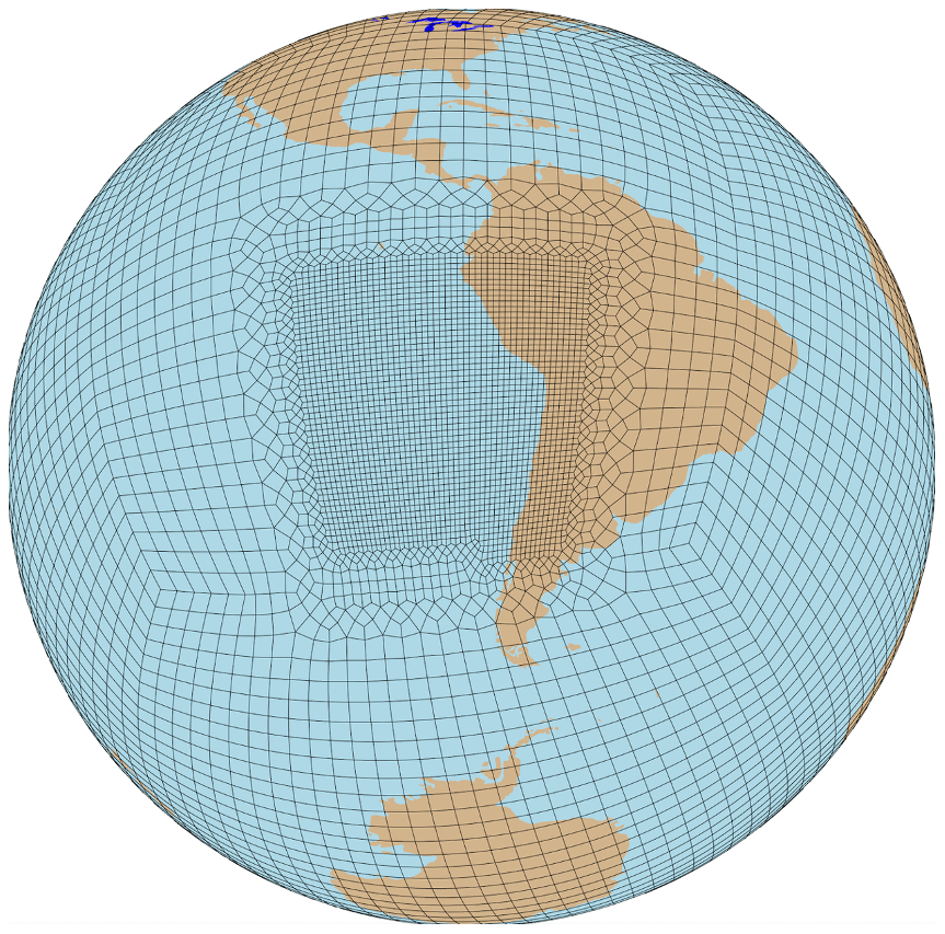
Figure 1 Depiction of the grid mesh used for the SEP-RRM-CNTL and SEP-RRM-FIVE simulations in this paper, with the ne120 resolution used within the refined region and the ne30 resolution used outside of this region. Note that each element shown contains additional 3×3 collocation cells.

The SEP-RRM consists of low-resolution (LR) and high-resolution (HR) regions and a transition area between them (Fig. 1). The HR grid is located over the heart of the southeastern Pacific stratocumulus area (Klein and Hartman, 1993; Bogenschutz et al., 2021; Lee et al., 2021). In addition, the HR grid includes much of the Andes Mountains over South America. We created the regionally refined grid with the offline software tool Spherical Quadrilateral Mesh Generator (SQuadGen; https://github.com/ClimateGlobalChange/squadgen, last access: 3 January 2023). The effective resolutions between the LR and HR regions are 1 and 0.25^∘, respectively. SEP-RRM has a total of 8351 quadrilateral elements on the globe, with these elements depicted in Fig. 1. As described in Dennis et al. (2012), the spectral element (SE) dynamical core operates on quadrilateral elements whose Gauss–Lobatto–Legendre (GLL) quadrature points form the physics columns in E3SM. The SEP-RRM covers approximately 4.5 % of the Earth's surface. In Sect. 3 we compare this number to the standard resolution configurations of E3SM; however, we note that the SEP-RRM is smaller in size to the RRM generated for the continental United States (CONUS; Tang et al., 2019), which contains 9905 elements.

2.3 Framework for Improvement by Vertical Enhancement

We utilize the novel Framework for Improvement by Vertical Enhancement (FIVE; Yamaguchi et al., 2017), which has been implemented into E3SM to improve marine stratocumulus clouds while substantially saving on computational cost (Lee et al., 2021). FIVE is unique because it allows for select processes or parameterizations to be run at a different vertical resolution to that of the host model. In the configuration of E3SM-FIVE used in this paper, three physics schemes are interfaced with vertically enhanced physics (VEP) to better represent low clouds, i.e., the CLUBB turbulence parameterization, the MG2 microphysics scheme, and the Rapid Radiative Transfer Module for GCM (RRTMG) longwave and shortwave radiation schemes (Iacono et al., 2008; Mlawer et al., 1997). In addition to the aforementioned physics schemes, large-scale vertical advection in the dynamical core is computed on the high-resolution grid, which is necessary to accurately balance entrainment via the turbulence scheme.

The tendencies calculated in VEP with a higher vertical resolution are averaged and applied to the host model (in this case E3SM) for prediction. The VEP calculation does not interfere with the order of the computation of processes in the host model, so the calculation of processes is not repeated between the host model and VEP. Lee et al. (2021) provides a detailed description of how FIVE is interfaced and implemented into E3SM.

3 Experiment design

We present results from a total of six experiments. Our low-resolution control model is E3SM run with the ne30 configuration (approximately 1^∘ horizontal resolution at the Equator) and with the standard 72 vertical layers (hereafter referred to ne30-CNTL). The high-resolution control model is E3SM run with the ne120 configuration (approximately 0.25^∘ horizontal resolution) and with the standard 72 vertical layers (hereafter referred to as ne120-CNTL).

In the first set of experiment simulations, we run them with FIVE turned on for each of the horizontal-resolution configurations (ne30 and ne120). We refer to these experiments as ne30-FIVE and ne120-FIVE. These simulations are the same as their CNTL experiment counterparts, except that FIVE is turned on, and thus the turbulence, microphysics, radiation, and large-scale vertical advection calculations are done on the VEP grid. In all FIVE simulations presented in this paper, the VEP grid represents an octupling of the vertical resolution compared to the standard vertical resolution in the lower troposphere (between 995 and 700 hPa; Fig. 2). Thus, the VEP grid contains 212 vertical levels, compared to the E3SM vertical grid of 72 levels. This is the exact vertical grid advocated by Bogenschutz et al. (2021) to achieve the best possible simulation of marine Sc.

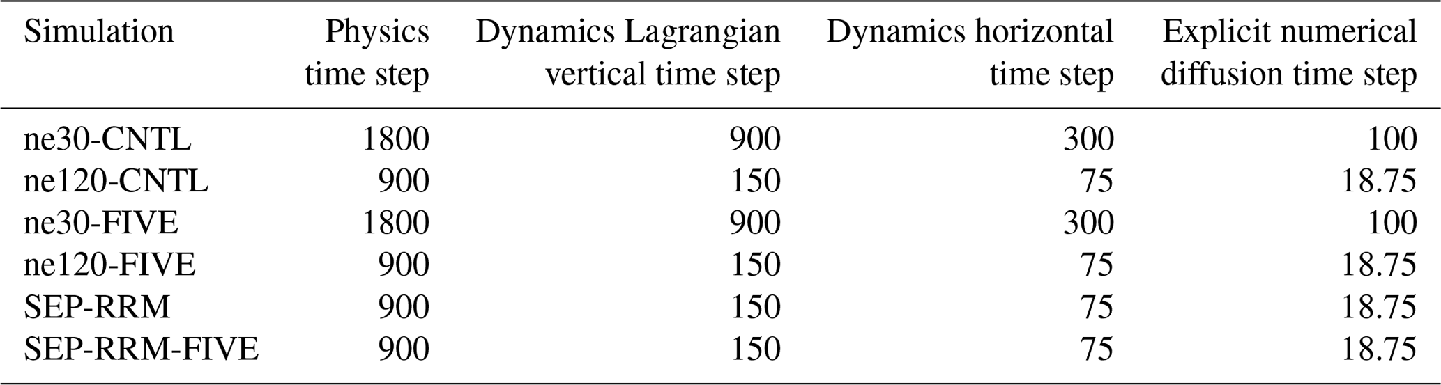
Table 1 Description of the simulations performed.

n/a: not applicable

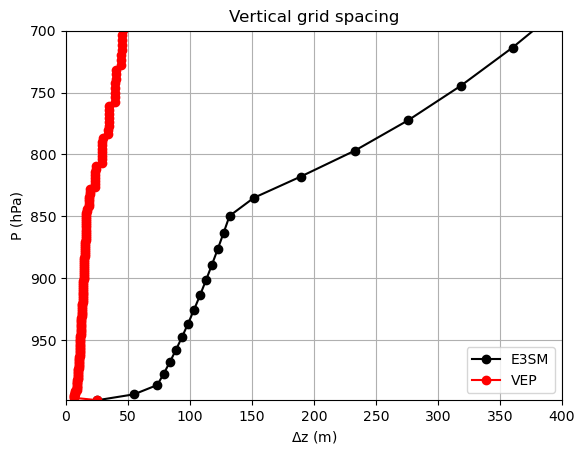
Figure 2 Estimated vertical grid spacing for the vertical grid used in E3SM (black curve) and for the vertically enhanced physics (VEP) used in the FIVE simulations in this paper.

For the second set of experiment simulations we use the newly generated southeastern Pacific regionally refined model (SEP-RRM) over the Peruvian region, both with the standard 72 vertical layers (hereafter referred to as SEP-RRM-CNTL) and with FIVE turned on, with the same vertical grid as the ne30-FIVE and ne120-FIVE experiments (hereafter referred to as SEP-RRM-FIVE). Table 1 provides details on the horizontal- and vertical-resolution configurations for each experiment.

For this study we treat ne30-CNTL as the default control simulation and the ne120-FIVE simulation as the high-resolution benchmark we strive to replicate within the southeastern Pacific with the SEP-RRM-FIVE simulation. We recognize that a true high-resolution benchmark simulation would involve running ne120 with 212 vertical levels. However, this simulation would have been computationally burdensome to perform (see Sect. 3.3). Furthermore, the work of Lee et al. (2021) has already established that simulations with FIVE can replicate the results of the high-resolution benchmark simulations with regard to the representation of marine stratocumulus.

In this study we perform atmosphere-only simulations forced by observed present-day climatology of aerosol emissions, greenhouse gases, sea surface temperatures (SSTs), and sea ice concentrations. The simulations use the interactive E3SM land model on the same grid as the atmosphere in each configuration. All simulations presented in Table 1 are run for 5 years.

Table 2 Description of the time steps used in each simulation.

3.1 Time steps

Table 2 presents the physics and dynamical time steps used for each simulation. We note that ne30-FIVE and ne120-FIVE simulations use exactly the same time step settings as their control simulation counterparts (ne30-CNTL and ne120-CNTL, respectively). Despite the fact that simulations with FIVE use 8 times the vertical resolution, compared to the standard E3SM 72-layer grid in the lower troposphere for several processes, no time step reduction is needed as the schemes interfaced with VEP grid use implicit schemes and are thus not constrained by the Courant–Friedrichs–Lewy (CFL) condition. Lee et al. (2021) report this as being a significant advantage of using FIVE versus refining the grid of the entire E3SM model (Bogenschutz et al., 2021) for the application of stratocumulus clouds, and this results in a major savings in terms of the computational cost.

We also note that simulations using SEP-RRM use the same time step settings as the ne120 simulations to retain the numerical stability in the high-resolution region. Though, we do note that this could introduce some degree of time step sensitivity in the LR region of our SEP-RRM experiments, as E3SM clouds and convection are known to exhibit some sensitivity to the time step (Wan et al., 2020).

In our study the ne30 (ne120) simulations are run with a 1800 s (900 s) physics time step. The dynamics use three layers of sub-stepping. For the ne30 (ne120) simulations, the Lagrangian vertical discretization time step is 15 min (2.5 min), the horizontal discretization time step is 5 min (75 s), and the explicit numerical diffusion time step is 100 s (18.75 s). As already stated, for the SEP-RRM simulations, we use the same physics and dynamics time step settings as the ne120 simulations.

3.2 Tunable parameters

We note that all simulations presented in this paper are run with exactly the same tunable parameters. While default ne30 and ne120 configurations of E3SMv1 are run with a slightly different set of tunable parameters in the CLUBB and Zhang–McFarlane (ZM) deep convection scheme (Zhang and McFarlane, 1995) to achieve radiation balance and optimal skill scores for coupled simulations, we chose to run all simulations with the default parameters for the ne30 configuration. This was a conscious decision that we made because otherwise it could be very difficult to disentangle whether the differences in our regime of interest (marine stratocumulus) would be due to tuning or resolution differences. This is similar to the approach that Caldwell et al. (2019) took when comparing low- and high-resolution E3SMv1 simulations when they wanted to avoid potential ambiguities that could arise from different tunable parameter sets.

In addition, it is common practice for RRM simulations to run with tunable parameters that are default for the HR mesh (Tang et al., 2019), with the argument being that they desire to mimic the HR behavior as closely as possible in their RRM runs. However, for our work, we feel that it is most appropriate to maintain the ne30 tunable parameters for SEP-RRM, regardless of whether or not we chose to maintain these tunable parameters for our ne120 simulations. The reason for this is that SEP-RRM is focused on a marine stratocumulus regime where the deep convection scheme is not active and most of the work is being done by the turbulence scheme of CLUBB. CLUBB is a scale-aware parameterization that has been shown to exhibit little sensitivity to the horizontal grid size (Larson et al., 2012), whereas the deep convection scheme in E3SMv1 is not scale aware. Therefore, since our area of interest does not contain deep convection, choosing to retain the ne30 tunable parameters so as not to modify the deep convection occurring in our LR region makes the most sense. Running the deep convective regime at ne30, and with ne120 tunable parameters, could potentially modify the Hadley circulation and thereby influence the results in our SEP-RRM domain.

Table 3 The computational expense of each simulation as run on Livermore Computing (LC) machines. SYPD stands for simulated years per day. Node hours are computed as nodes used multiplied by the number of hours required to simulate 1 year.

3.3 Computational cost

Table 3 displays the computational cost of each simulation. All of the runs presented in this paper were performed on Livermore Computing's (LC) Quartz machine. Table 3 provides the node hours required for each simulation per simulated year and is computed as the total number of nodes used multiplied by the hours to obtain a simulated year. As expected, the ne30-CNTL simulation is the least computationally expensive, while the ne120-FIVE simulation is the most computationally expensive (i.e., 2 orders of magnitude more expensive than ne30-CNTL).

In general, runs using FIVE tend to be 2–3 times as expensive as their CNTL run counterparts using the same horizontal resolution. As reported by Lee et al. (2021), the added cost associated with FIVE is small when compared to the cost of running the entire model at a high vertical resolution, which would have yielded costs that are an entire order of magnitude higher. We estimate that a simulation with the ne120 resolution and 212 vertical levels would have cost nearly 300 000 node hours per simulated year, with the majority of this expense being attributed by the need to run with a very small time step. Thus, without FIVE, this would make running ne120 simulations with a high vertical resolution infeasible for this study.

Table 3 demonstrates that while both SEP-RRM and SEP-RRM-FIVE are roughly 3 times more expensive than ne30-CNTL and ne30-FIVE, respectively, they are both an order of magnitude less expensive than their ne120 counterpart simulations. This represents the reasonable tradeoff in cost that is expected with these RRM simulations (Tang et al., 2019).

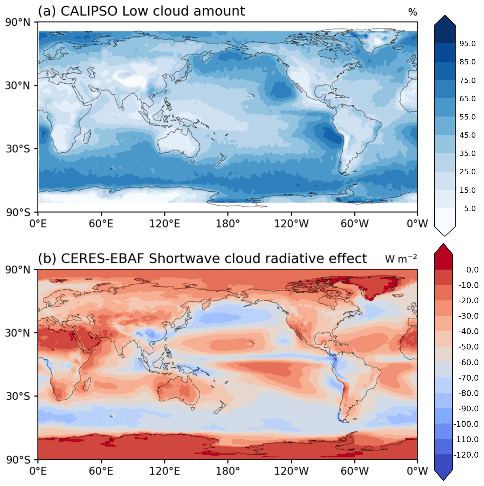
Figure 3 (a) Low cloud amounts from Cloud-Aerosol Lidar and Infrared Pathfinder Satellite Observation (CALIPSO) from January 2007 to January 2010 and (b) shortwave cloud radiative effect (SWCRE) from Clouds and Earth's Radiant Energy System (CERES) Energy Balance and Filled (CERES-EBAF) product from 2001 to 2018.

4 Results

4.1 Low cloud climatology

Since our target regime is subtropical marine stratocumulus, we will first focus on results relating to the simulated low cloud amount and the shortwave cloud radiative effect (SWCRE). Figure 3 displays the climatological observed values for these two quantities. Observations for low cloud amounts are provided from Cloud-Aerosol Lidar and Infrared Pathfinder Satellite Observation (CALIPSO) from January 2007 to January 2010, while those for SWCRE are provided by the Clouds and Earth's Radiant Energy System (CERES) Energy Balance and Filled (CERES-EBAF) product from January 2001 to January 2018. Focusing on the subtropics, we see three prominent local maxima of low cloud amounts off the western coasts of South America, California, and Namibia, with two lesser maxima near the western coast of Australia and North Africa. These cloud maxima are due to the subtropical marine stratocumulus (Klein and Hartman, 1993) and the areas also indicated in the observed figure of SWCRE as being areas of strong reflectivity.

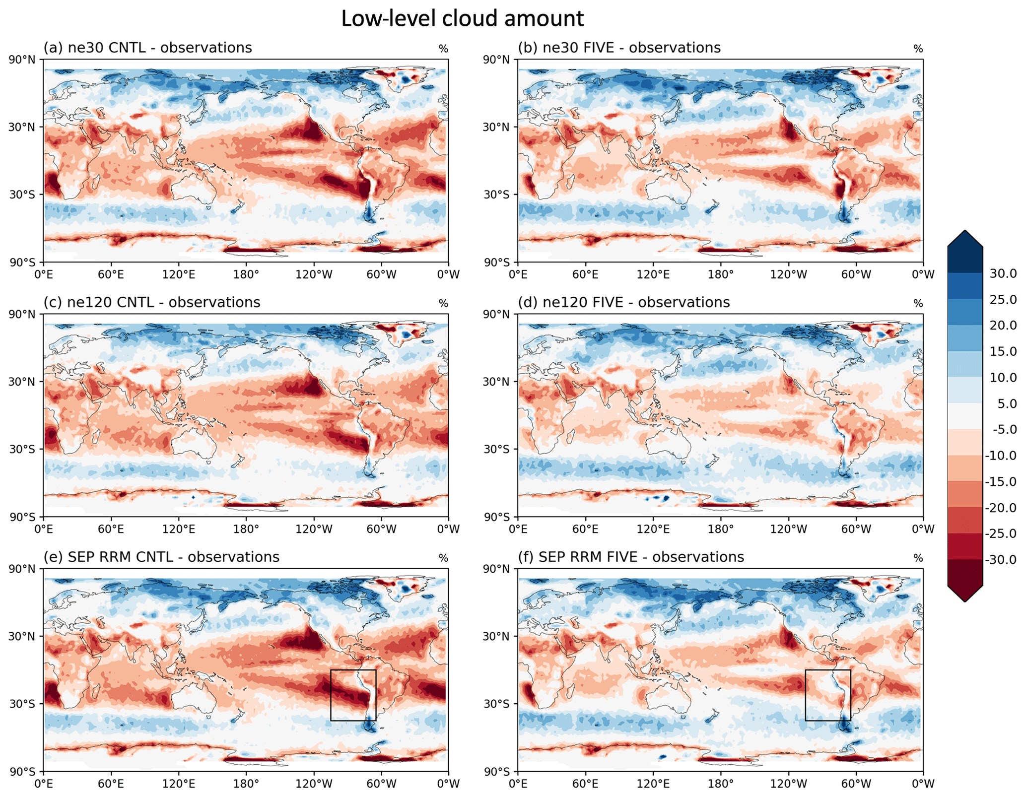
Figure 4 Annual low cloud amount biases computed relative to observations for (a) ne30-CNTL, (b) ne30-FIVE, (c) ne120-CNTL, (d) ne120-FIVE, (e) SEP-RRM-CNTL, and (f) SEP-RRM-FIVE. The box in panels (e) and (f) represents the area of the refined mesh in these simulations.

Figure 4 displays the geographical bias of the simulated low-level cloud amount for our six configurations computed relative to CALIPSO observations. We note that our E3SM simulations use the Cloud Feedback Model Intercomparison Project (CFMIP) Observation Simulator Package (COSP; Bodas-Salcedo et al., 2011), which contains several independent satellite simulators to diagnose model clouds in a similar way to how satellites would view an atmosphere. This allows for an apples-to-apples comparison of our simulated low cloud amount with CALIPSO observations. Low-level cloud amount represents the vertically integrated cloud fraction from the surface to 680 hPa, as defined in Chepfer et al. (2008). As already indicated by Bogenschutz et al. (2021) and Lee et al. (2021), the ne30-CNTL (Fig. 4a) simulation is characterized by a dearth of low-level cloud in the three main subtropical stratocumulus regions. This is a bias endemic to most GCMs and is not specific to E3SM. While the increasing vertical resolution through FIVE (ne30-FIVE) helps to ameliorate the bias associated with low cloud for stratocumulus cloud that resides offshore (Fig. 4b), biases near the coast remain. In addition, while increasing horizontal resolution (ne120-CNTL) alone appears to marginally improve biases of stratocumulus cloud along the coast, it does little towards reducing the overall bias associated with this cloud regime.

The concurrent increase in the horizontal and vertical resolutions (ne120-FIVE) has the most substantial impact on the local bias reduction in subtropical marine stratocumulus cloud (Fig. 4d; Lee et al., 2022). Here we seek to answer the question of whether RRM can help to replicate these results for one of the subtropical stratocumulus regimes – specifically that residing in the SE Pacific.

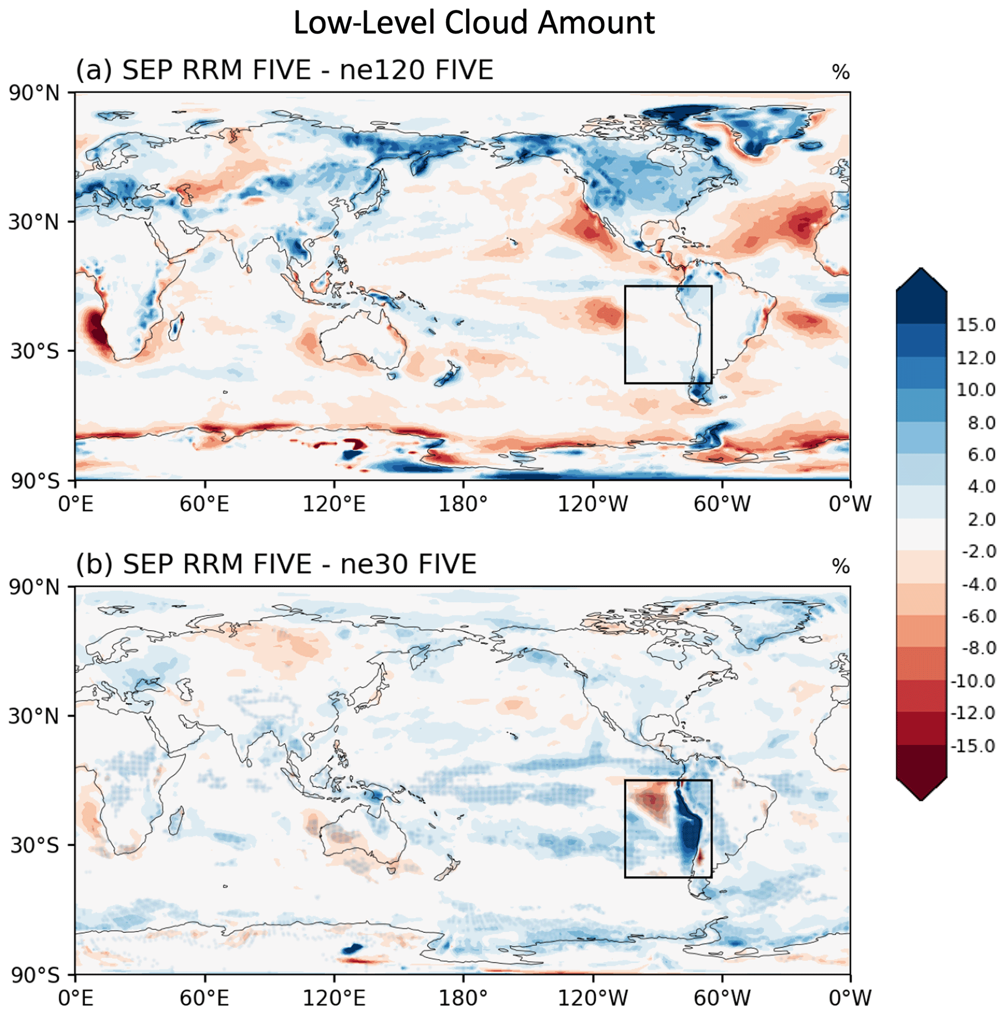
Figure 5 Differences in low cloud amount for the SEP-RRM-FIVE simulation calculated with respect to the (a) ne120-FIVE and (b) ne30-FIVE simulations. The bounded box represents the area of the refined mesh in these simulations. In panel (b), the light blue stipple indicates locations where differences are statistically significant at the 95 % confidence level.

Figure 4e–f display the low-level cloud amount biases for the SEP-RRM-CNTL and SEP-RRM-FIVE simulations, respectively. Our focus region is the stratocumulus in the southeastern Pacific, as denoted by the bounding box in these figures. The hope is that the bias displayed within the bounding box of Fig. 4e (SEP-RRM-CNTL) resembles that of the corresponding region of Fig. 4c (ne120-CNTL) and that the same applies for the sets of simulations using FIVE (Fig. 4f versus Fig. 4d). While the degree to which the results can be replicated in the RRM simulations will be quantified in further figures, it appears that this can be successfully done. This is especially obvious when comparing the SEP-RRM-FIVE results in the SEP to that of the ne120-FIVE simulation where the local bias reduction is substantial and very similar when comparing these two simulations.

Figure 5 directly compares the SEP-RRM-FIVE simulation with the ne120-FIVE and ne30-FIVE simulations for the refined and outer regions. Focusing on the differences with respect to the high-resolution benchmark ne120-FIVE simulation (Fig. 5a), we see virtually no difference in the change in low-level cloud amount within the refined region, while there are relatively large differences around the rest of the globe, including the subtropical stratocumulus regions near California and Namibia. On the other hand, the differences with respect to ne30-FIVE (Fig. 5b) show nearly the opposite behavior, with relatively large differences in the refined region and a smaller difference in the rest of the globe. Overall, this is the expected result and provides encouraging evidence that the new SEP RRM is performing as hypothesized. In Fig. 5b, since the horizontal and vertical resolutions in the outer domain are identical, this figure could presumably show the global impact of reduced stratocumulus biases in the SEP. To explore this, the stippled areas indicate where differences are statistically significant at the 95 % confidence level. This suggests improving stratocumulus biases in the SEP could have implications on the simulation within the Intertropical Convergence Zone (and associated double ITCZ problem) and Southern Hemisphere storm tracks. However, we caution that these two simulations do have different time step settings (Table 2) which could be contributing to these differences. In addition, these simulations use prescribed SSTs which could potentially be muting the global impact. Exploring the global effects from improved marine stratocumulus biases is something that could be pursued in future work. The SEP-RRM-FIVE configuration would provide the ideal framework to do such a study.

Figure 6 (a) Bias and (b) root mean squared error (RMSE) of low-level cloud amounts for each simulation computed relative to CALIPSO observations. Each skill metric is computed for the global domain (left) and the SE Pacific region (right), as bounded by the box in Fig. 4e. We note that, for skill scores computed for the SE Pacific region, only ocean columns (which we define as columns having a less than 0.5 land fraction) are considered to focus on scores for marine boundary layer clouds. Hatched bars represent simulations run with FIVE.

The bias and root mean squared error (RMSE) scores for low-level cloud amount can be found in Fig. 6. Here we have segregated the scores into two categories, namely one which includes the bias and RMSE for the entire globe for each configuration and the other which represents the skill scores exclusively for oceanic columns in SE Pacific region. Focusing first on the global skill scores, we see that all simulations using FIVE are characterized by an increase in the global low-level cloud. This is mostly due to an increase in stratocumulus and trade wind cumulus clouds across the entire subtropical oceans when FIVE is activated. However, in terms of RMSE, there is generally a less dramatic difference between the simulations, though the simulations using FIVE score slightly better than their CNTL counterparts.

Focusing on the skill scores for the SE Pacific region, however, we see a much more distinct behavior as the horizontal and vertical resolution changes. For the SE Pacific the expectation is that the skill metrics would be very similar for the SEP-RRM-CNTL and ne120-CNTL set of simulations and the SEP-RRM-FIVE and ne120-FIVE set of simulations. For both the bias and RMSE skill scores we see that both sets of simulations agree very well with each other, suggesting that the SEP-RRM is able to replicate the behavior of the ne120 configurations for marine stratocumulus well.

Beyond demonstrating the effectiveness of the SEP-RRM in replicating the behavior of high-resolution runs for marine stratocumulus, Fig. 6 also illustrates the importance of concurrent increases in the horizontal and vertical resolutions when simulating marine Sc. All three simulations that use the default 72 vertical levels for all processes greatly underestimate cloud cover with associated large errors for this region. Simply increasing the horizontal resolution, as evident in the ne120-CNTL simulation, does little to ameliorate error. The introduction of FIVE in the low-horizontal-resolution configuration, ne30-FIVE, demonstrates a noticeable reduction with regard to the bias and error. However, it is not until the horizontal and vertical resolutions are concurrently increased (ne120-FIVE and SEP-RRM-FIVE) that substantial reductions in the bias and RMSE are seen.

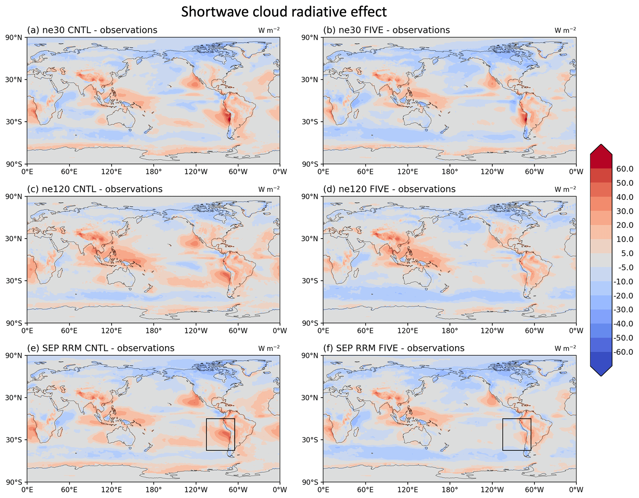
Figure 7 Same as Fig. 4 but for shortwave cloud radiative effect.

We are most concerned with the simulation of low clouds because of their impact on shortwave radiation. Therefore, we also examine the simulation of SWCRE for each simulation. The annually averaged observed SWCRE can be found in Fig. 3b, with the differences for each simulation compared to observations found in Fig. 7. In general, the same behavior found in the analysis with low-level cloud amount can be found in SWCRE. The ne30-CNTL simulation is characterized by too little reflectivity in the subtropics, with bull's eyes on the subtropical marine Sc. These biases are only marginally reduced in the ne120-CNTL simulation, with slight improvements seen in the coastal regions of the marine Sc. This follows the general conclusions of Caldwell et al. (2019). While the introduction of FIVE to the ne30 simulation goes a long way in helping to ameliorate the SWCRE biases in the subtropics, it is not until the horizontal resolution is concurrently increased in the ne120-FIVE simulation that large reductions in the biases are found. In addition, similar to the result of low-level cloud amount, the results for the two SEP-RRM runs (CNTL and FIVE) appear to behave as expected, with bias patterns and magnitude that look very similar to each ne120/ne30 counterpart within the refined/outer region.

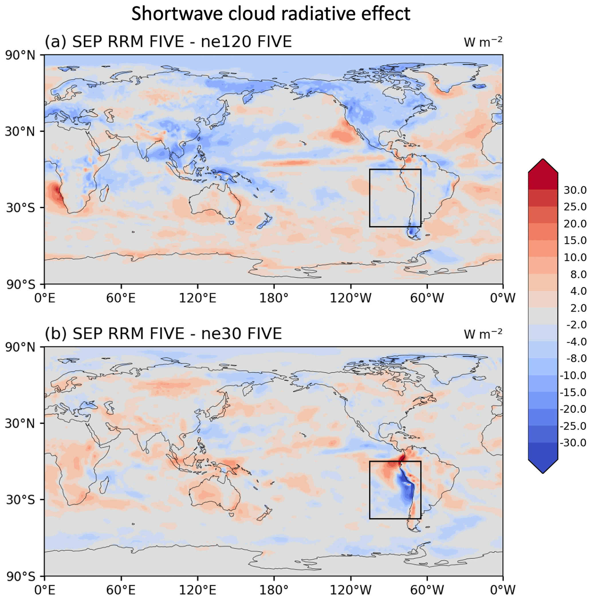
Figure 8 Same as Fig. 5 but for shortwave cloud radiative effect.

To exploit the behavior of the of the SEP-RRM for SWCRE we directly compare the SEP-RRM-FIVE simulation with the counterpart ne120-FIVE (Fig. 8a) and ne30-FIVE (Fig. 8b) simulations. Similar to the low-level cloud amount, we see an excellent agreement of SWCRE with the ne120-FIVE experiment within the refined region and relatively large differences for the rest of the globe. Conversely, there are large differences in SWCRE with the ne30-FIVE experiment within the refined region. Again, while this is the result we hoped for, a very interesting feature is the robustness of the simulated SWCRE within the refined region for SEP-RRM-FIVE with respect to ne120-FIVE, despite there being large differences in the simulated SWCRE in the rest of the globe. This is especially true in the tropics where there are relatively large differences in SWCRE. While this is not especially surprising, given that the resolutions of these two simulations are different in these regions and will cause a change in the simulated convection due to the convective parameterization of E3SM not being scale aware, it is often thought that a modified deep-convection simulation will alter the large-scale circulation, thereby inducing changes to the simulated marine Sc. However, here we see that refining the local resolution is the first-order sensitivity for marine Sc.

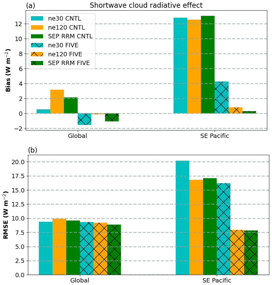
Figure 9 Same as Fig. 6 but for shortwave cloud radiative effect computed relative to CERES-EBAF observations.

Focusing on the quantitative skill score metrics for SWCRE, we see that most simulations have minimal bias with respect to global domain (Fig. 9a). This is not surprising since ne30-CNTL was tuned to achieve radiation balance, though the remainder of the simulations which were not tuned tend to exhibit either a slightly positive or negative bias. Conversely, when just examining the SE Pacific region, we see that all three CNTL simulations exhibit a large positive bias. This bias is substantially reduced with the introduction of FIVE but is especially better and comparable for the ne120-FIVE and SEP-RRM FIVE simulations, as expected. The global RMSE skill scores for all six simulations are very similar for the global domain (Fig. 9b) but again demonstrate considerable differences for the SE Pacific region. Here we see that ne30-CNTL has the largest error, with the ne120-FIVE and SEP-RRM-FIVE simulations having the best scores and being very comparable to one another.

Figure 10 Profiles of (a) cloud fraction, (b) cloud liquid water, (c) longwave heating rate, and (d) vertical velocity variance predicted by CLUBB for each simulation averaged over 5 years. The profiles are spatially averaged over the domain used for regional refinement, as illustrated in Fig. 1. Only oceanic columns are included in the averages and are defined as those with a land fraction of less than 0.5.

Figure 10 presents 5-year annual averaged profiles for oceanic columns from the SEP RRM domain. The profiles of cloud fraction and cloud liquid amount (Fig. 10a and b) demonstrate that the simulations including FIVE tend to simulate thicker cloud decks that contain more coverage and liquid water relative to their CNTL counterpart configurations. This is in general agreement with the results presented in Lee et al. (2021). Here we demonstrate that the SEP-RRM-FIVE simulation bears a remarkable agreement to the simulation characteristics of ne120-FIVE. This agreement is also present in the averaged profiles for the longwave cooling rate and the vertical velocity variance ($\stackrel{\mathrm{‾}}{w^{\prime \mathrm{2}}}$) predicted by CLUBB. The agreement provided by SEP-RRM-FIVE and ne120-FIVE suggests that the simulated turbulence and cloud top feedback at the process level are roughly the same between the two simulations.

Thus far we have demonstrated that the SEP-RRM is effective in replicating the results that global high-resolution simulations provide but with a refined patch over the region of interest. We have also demonstrated that the combination of an increased horizontal resolution and vertical resolution (through the use of FIVE) is required to produce the best possible results with regards to the simulation of marine stratocumulus. Bogenschutz et al. (2021) found that a LES-like vertical resolution was needed to achieve satisfactory simulation of marine stratocumulus, and the primary mechanism was a positive feedback between the cloud-top cooling, turbulence, and cloud macrophysics processes. They found that the high vertical resolution was better able to resolve the sharp cloud-top inversion, which leads to a more accurate representation of the height of maximum cloud and liquid when compared to satellite retrievals. This helps to generate copious amounts of cloud-top cooling, which encourages turbulence of the boundary layer to be primarily driven from cloud top. The lower vertical-resolution simulations lacked sufficient cloud cover, allowed an abundance of solar radiation to reach the surface during the daytime, and caused turbulence generation to be primarily surface driven. In turn, this led to decoupled profiles of $\stackrel{\mathrm{‾}}{w^{\prime \mathrm{2}}}$ and positive values of the third moment of the vertical velocity ($\stackrel{\mathrm{‾}}{w^{\prime \mathrm{3}}}$), which were more indicative of a shallow cumulus boundary layer and helped to further thin the cloud deck, as vertical velocity skewness (defined as ($\stackrel{\mathrm{‾}}{w^{\prime \mathrm{3}}}/\stackrel{\mathrm{‾}}{w^{\prime \mathrm{2}}}{)}^{\mathrm{3}/\mathrm{2}}$) is used in CLUBB to parameterize the cloud fraction and liquid water mixing ratio (Golaz et al., 2002; Larson et al., 2002). On the other hand, the higher vertical resolution case, where turbulence is primarily generated from the cloud top, produces neutral or negative values of vertical velocity skewness, which encourages more abundant cloud formation and a positive feedback.

Lee et al. (2021) found that this positive feedback loop to improve stratocumulus cloud could be replicated in FIVE as long as CLUBB, microphysics, radiation, and large-scale vertical advection are all interfaced with the vertically enhanced physics. Finally, Lee et al. (2022) found a substantial improvement to the simulated coastal stratocumulus with concurrent increases in the horizontal and vertical resolutions to better capture the coastlines and sharp terrain gradients, which is particularly important for the southeastern Pacific stratocumulus region, given its proximity to the Andes Mountains.

4.2 Seasonal cycle of low clouds in the southeastern Pacific

While we have thus far demonstrated the ability of SEP-RRM to represent stratocumulus through the climatological mean, in this section we seek to address how our highest-resolution configuration (ne120-FIVE) can represent the seasonal cycle of low clouds in the southeastern Pacific and how well the RRM-FIVE configuration can replicate this. Because we found that the simulations with FIVE are required to obtain superior results for the climatological mean, we will only focus our analysis on comparing the ne120-FIVE and SEP-RRM-FIVE simulations against observations and the ne30-CNTL model.

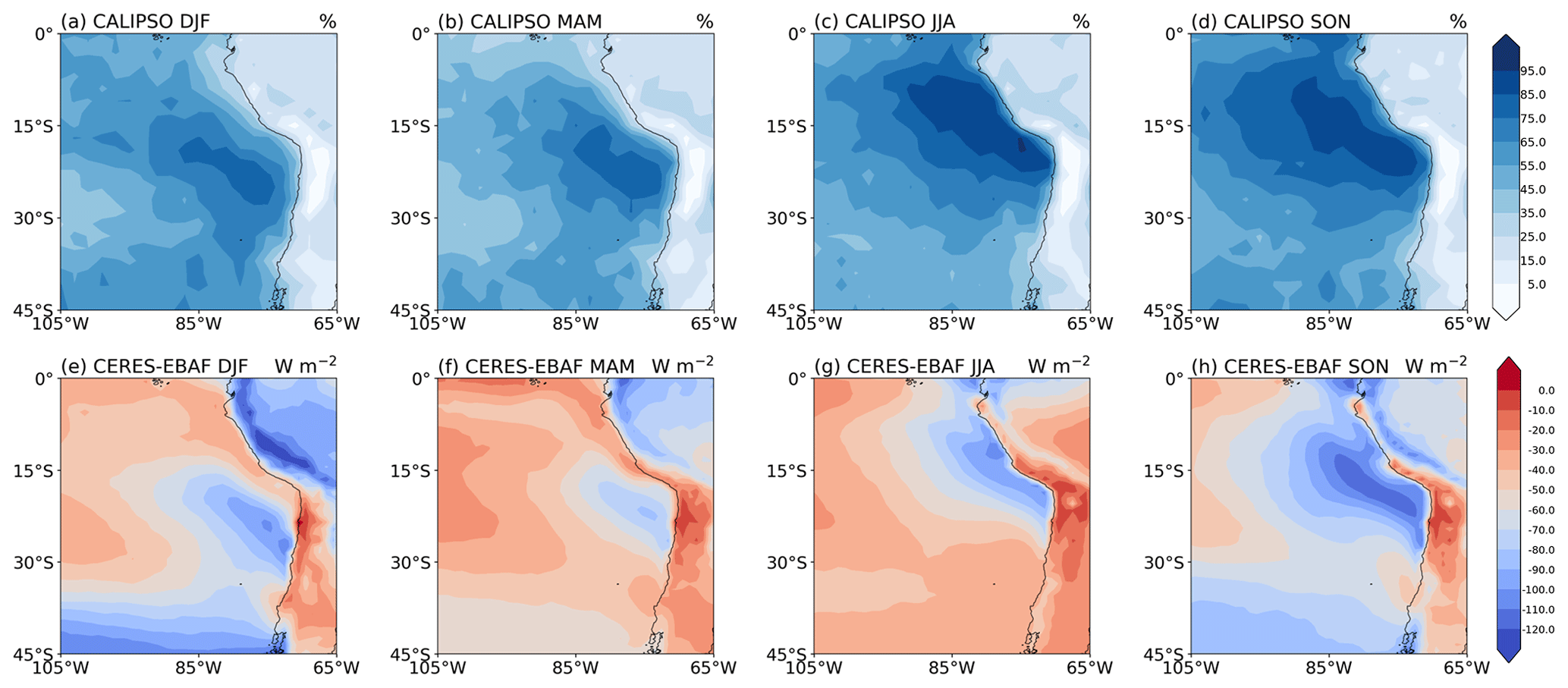
Figure 11 Observed low-level cloud amount from CALIPSO (a–d) and shortwave cloud radiative effect from CERES-EBAF (e–h), averaged over December, January, and February (DJF; a, e), March, April, and May (MAM; b, f), June, July, and August (JJA; c, g), and September, October, and November (SON; d, h).

Figure 11 displays the observed seasonal cycle of the low-level cloud amount and SWCRE for the SE Pacific region that is subject to regional refinement in our simulations. The figures are segregated by season, namely boreal winter (December, January, and February; DJF), spring (March, April, and May; MAM), summer (June, July, and August; JJA), and autumn (September, October, an November; SON). While marine stratocumulus persists over the ocean in all seasons for this region, the climatological maximum occurs during SON, with a minimum during MAM. The JJA and SON seasons see a relative northward shift and maximum of coastal Sc along the coast of Peru, while DJF and MAM see a southward shift in marine Sc and a maximum of coastal Sc along the Chilean coast.

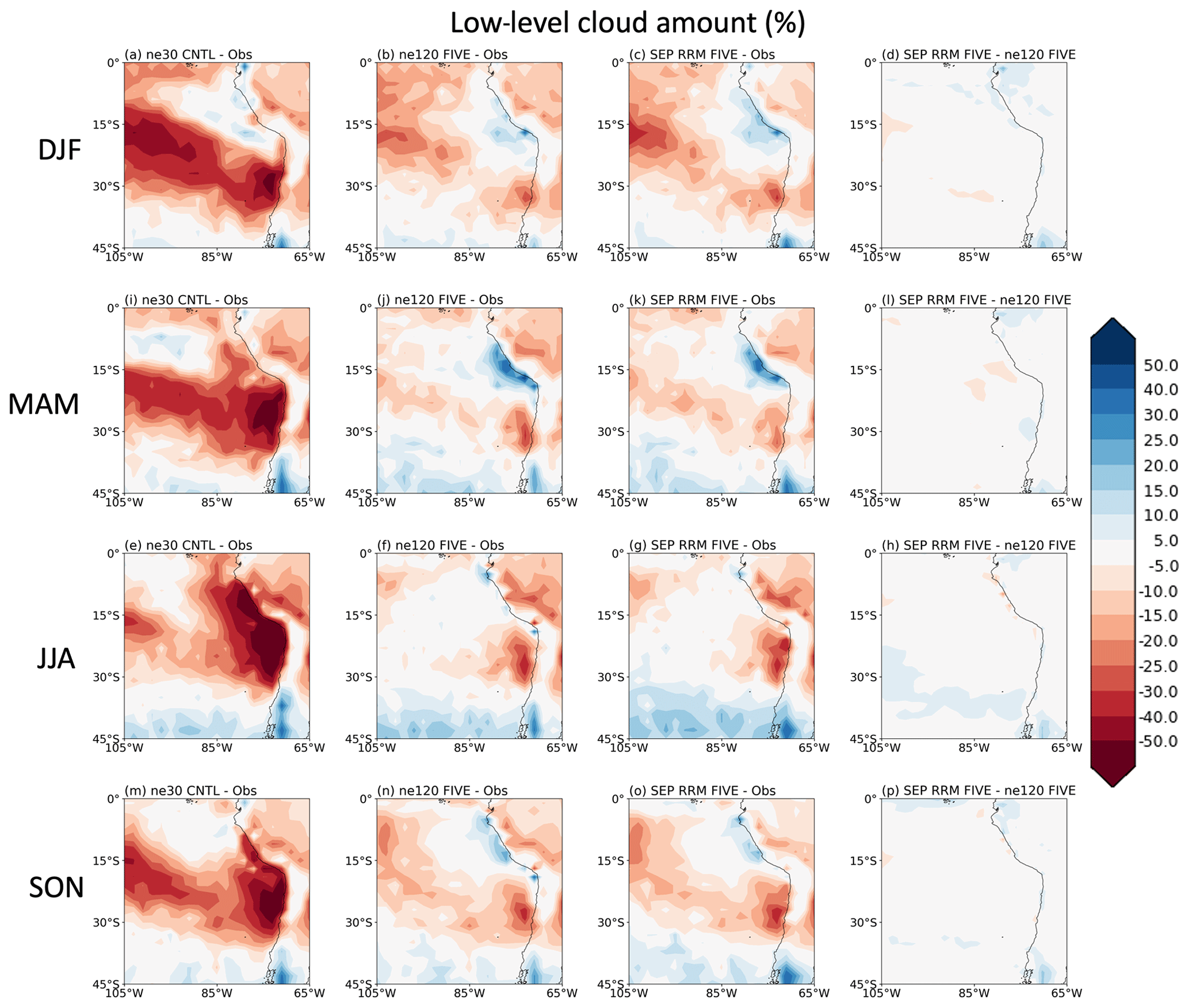
Figure 12 Differences in low-level cloud amount computed relative to CALIPSO observations for ne30-CNTL (a, i, e, m), ne120-FIVE (b, j, f, n), and SEP-RRM-FIVE (c, k, g, o). Also displayed are the differences in SEP-RRM-FIVE computed relative to ne120-FIVE (d, l, h, p). Results are displayed for the DJF (a–d), MAM (i–l), JJA (e–h), and SON (m–p) seasons.

Differences in low cloud amount for the ne30-CNTL and ne120-FIVE simulations, computed relative to CALIPSO observations, are displayed in the first two columns of Fig. 12. It is clear that the ne30-CNTL simulation systematically underestimates low-level cloud for all seasons. This bias is most severe along the coast but also persists offshore, particularly during DJF and MAM. It is also noteworthy that widespread regional deficits along the coast upwards of 50 % exist during the peak seasons of JJA and SON, highlighting the severity of the Sc bias in E3SM that is not as obvious when only considering the global annual averages.

Examining the biases of the ne120-FIVE simulation, we see noteworthy improvement for all seasons, though some biases still remain to a degree. The most stubborn bias in the ne120-FIVE simulation is slight underestimation of low cloud along the Chilean coast for all seasons, though the magnitude of this bias is significantly smaller when compared to ne30-CNTL. In addition, whereas ne30-CNTL has a persistent underrepresentation of low clouds along the Peruvian coast, ne120-FIVE now has a slight overestimation of low-level clouds in this area during the MAM and SON seasons. Can SEP-RRM-FIVE replicate the improvements that ne120-FIVE demonstrates at the seasonal timescale? An examination of the biases relative to observations of SEP-RRM-FIVE (third column of Fig. 12) shows very similar bias patterns and magnitude to that of ne120-FIVE. The similarity of these two simulations is further confirmed when looking at the differences between SEP-RRM-FIVE and ne120-FIVE (fourth column of Fig. 12), which shows near-perfect agreement for all seasons. This further demonstrates the ability of RRM to replicate the high-resolution behaviors of a Sc regime.

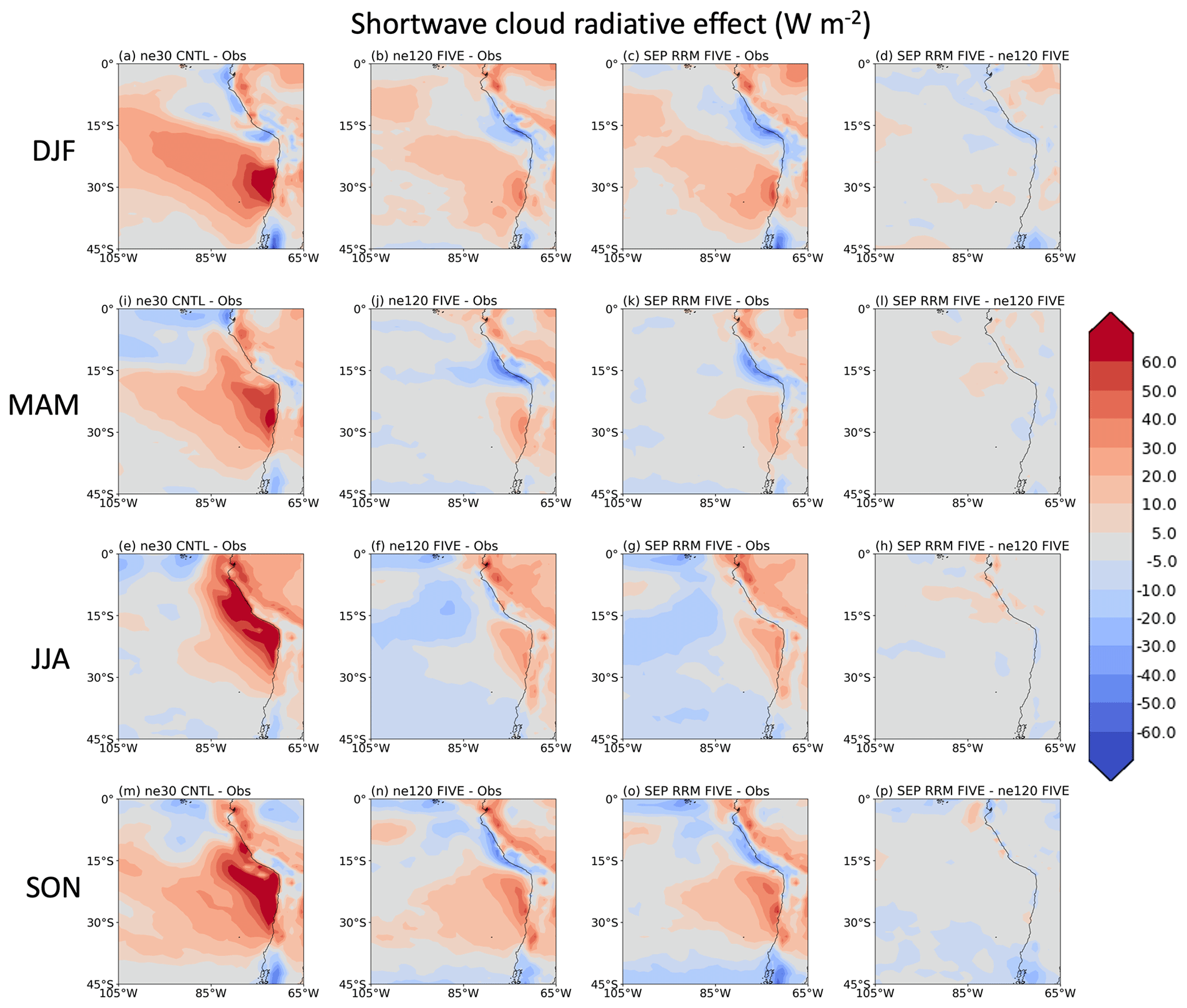
Figure 13 Same as Fig. 12 but for shortwave cloud radiative effect.

Figure 13 displays the seasonal biases for the SWCRE. Overall, we see the expected result, given the biases presented for the low-level cloud amounts in Fig. 12. The ne30-CNTL simulation suffers from systematic bias of too little reflectivity that is most severe along the coast. Whereas the ne120-FIVE simulation improves upon this bias, it is notable that relatively large biases exist for this configuration both along the coast and offshore during the DJF and SON seasons. These biases are somewhat larger than the biases in the low-level cloud amount may suggest and point to the need for further parameterization improvements or tuning of the parameterization suite in E3SM to enhance the agreement with observations. In addition, further refinement of the vertical grid in VEP could lead to additional improvements, as suggested in Lee et al. (2021). However, similar to the analysis of low-level cloud amount, we see that the SEP-RRM-FIVE has excellent agreement with the much more expensive ne120-FIVE simulation (third and fourth columns of Fig. 7).

4.3 General climatology

This paper has been focused on the simulation of low-level marine clouds and their sensitivity to horizontal and vertical resolutions. However, it is important to assess the credibility of the overall simulated global climate to ensure that potential significant degradations in our experimental simulations are not providing unrealistic boundary conditions to our region of interest. We have assessed the credibility of the global simulated climate and have verified that no configuration contains any major pathological error or bias relative to ne30-CNTL. Here, we succinctly present our findings to support this conclusion.

Table 4 Top-of-atmosphere radiation budgets for the simulations performed. All units are given in watts per meter squared (W m⁻²). Note that LWCRE is for longwave cloud radiative effect.

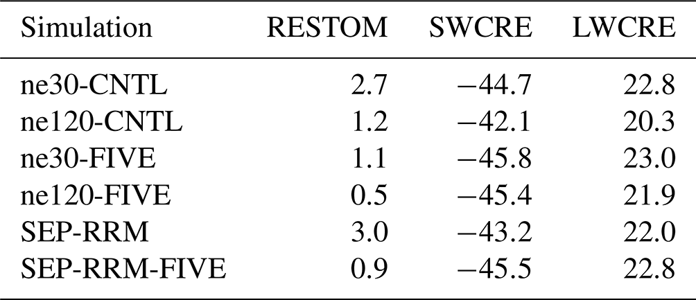
Table 4 displays the top-of-atmosphere radiation budget for each experiment. Since these simulations use present-day forcing, we cannot expect a near-zero top-of-atmosphere energy balance. The ne30-CNTL simulations show an energy balance (RESTOM) of about 2.77 W m⁻². As already noted, we chose to run our ne120 simulations with the same tunable parameters as the ne30 simulations; therefore it is not surprising that these simulations differ in terms of their RESTOM values. Therefore, it is clear that any experiment simulation presented in this paper would be subjected to some tuning to achieve radiation balance should they be run in coupled mode, which could have some minor impact on the overall results presented in this paper.

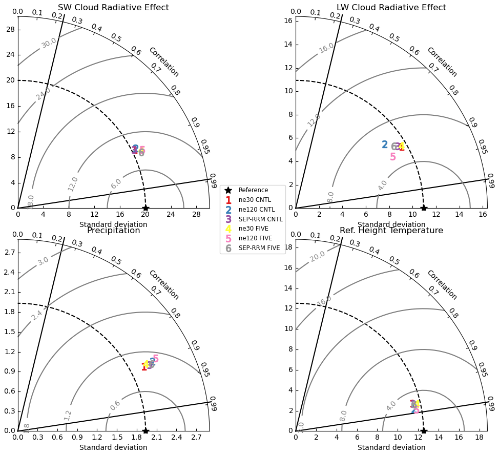
Figure 14 Taylor diagrams depicting the global skill for each simulation for 5 years for shortwave cloud radiative effect (SWCRE), longwave cloud radiative effect (LWCRE), precipitation, and reference height temperature.

Figure 14 displays diagrams (Taylor, 2001) to succinctly compare model skill between the various experiment simulations for climatologically important variables such as SWCRE, LWCRE, precipitation, and reference temperature height. It is expected that ne30-CNTL would tend to produce the best results, since that simulation was tuned for E3SM production runs, and overall, this does appear to be the case here. However, all simulations tend to produce similar skill score metrics, further highlighting the fact that our experimental simulations are credible at the global scale. The biggest spread between the simulations appears to be for LWCRE and precipitation, where the ne120 simulations tend to show slightly less skill than the remainder of the simulations.

5 Conclusions

In this paper we develop a novel framework that refines the horizontal resolution of E3SM in the southeastern Pacific (SEP) while simultaneously refining the vertical resolution for select physics processes to reduce biases related to subtropical marine stratocumulus clouds. Our regional refined mesh (RRM) is centered off the coast of Peru and Chile, with an effective resolution of 0.25^∘, with the standard 1.0^∘ resolution covering the remainder of the globe. Our vertical-resolution refinement takes advantage of the Framework for Improvement by Vertical Enhancement (FIVE; Yamaguchi et al., 2017) to run E3SM's turbulence, microphysics, and radiation schemes on a much higher vertical resolution than the standard 72-layer E3SM grid. In this study we refine the vertical resolution to near 10 m in the lower troposphere for FIVE, which is representative of the resolution often used in LES for stratocumulus.

We find that the superior results produced by the high-resolution benchmark simulation (ne120-FIVE) are reproduced with great fidelity in the SEP region with our new SEP-RRM-FIVE configuration. In addition, the computational cost of the SEP-RRM-FIVE simulation is much reduced compared to ne120-FIVE, as expected, as it uses only 5 % of the computational resources of the high-resolution benchmark simulation. We recognize that, in this paper, we did not perform a true high-resolution benchmark, which would have involved running ne120 with 212 vertical levels, due to the excessive computational cost that would demand (Bogenschutz et al., 2021) and due to the fact that it has already been established that FIVE can reproduce the results for marine stratocumulus clouds compared to running a high vertical resolution for all processes (Lee et al., 2021). However, we project that, compared to a true high-resolution benchmark (ne120 horizontal resolution with 212 vertical levels), the cost of the SEP-RRM-FIVE configuration would represent only 0.05 % of the total cost of said simulation. This highlights the major cost benefits of using horizontal mesh refinement in conjunction with FIVE to target marine stratocumulus biases.

We demonstrate that concurrent increases in the horizontal and vertical resolutions are needed for a substantial reduction in the stratocumulus biases and realistic seasonal representation in the Peruvian region. We also show that the SEP-RRM-FIVE configuration can replicate the results of the ne120-FIVE configuration in this regard. This provides an affordable framework to perform experiments related to climate sensitivity and aerosol affects in a simulation with improved and realistic stratocumulus representation. Nevertheless, we recognize that this work refines only one stratocumulus region. However, it is completely feasible for one to horizontally refine multiple regions of the globe. For instance, one could conceivably refine the Californian, Peruvian, and Namibian low-cloud regions simultaneously. Given the relatively small horizontal extent that marine stratocumulus cover, the size requirement of the horizontal refined patches would likely still allow for big computational cost savings.

Another opportunity to increase the throughput of these simulations is to only activate FIVE in the geographical regions of interest and run with the standard 72-layer grid for all columns and processes outside of these regions. Currently, the FIVE implementation into E3SM can only be activated in all (or no) columns globally and with the same number of VEP levels. An extension to make FIVE activate only in select columns is theoretically possible but made challenging by the fact that all parameterizations in E3SM (i.e., CLUBB, MG2, and RRTMG), and likely in most GCMs, are initialized with the same number of vertical levels in all columns and assumes that all columns will use the same number of vertical levels throughout the duration of the simulation. This provides a software engineering challenge, and one that would likely be worthwhile to overcome, given that stratocumulus are particularly sensitive to vertical resolution and cover a small portion of the globe.

Finally, while our prototype framework has been implemented in the context of the conventionally parameterized GCM, we expect this framework to be useful for the next generation of GCMs as we gradually move to cloud-resolving scales. In terms of the vertical resolution, most global cloud-resolving models (GCRMs; i.e., Caldwell et al., 2021) run with relatively coarse vertical resolution in the lower troposphere. Thus, this highlights the importance of tools such as FIVE to ensure that the minimum vertical resolution requirement to simulate stratocumulus is met (Lee et al., submitted) in these models. Though GCRMs often have horizontal resolutions of the order of 3 km, which is enough to adequately resolve the coastlines, boundary layer turbulence is still not resolved at these resolutions. While some GCRMs contain sufficient boundary layer parameterizations to represent stratocumulus reasonably enough, refining a horizontal mesh over a particular stratocumulus region could allow for simulations where the large eddies are resolved, providing a computationally affordable framework to assess the performance and potential benefits of LES in the context of a global simulation.