Adding sea ice effects to a global operational model (NEMO v3.6) for forecasting total water level: approach and impact

In operational flood forecast systems, the effect of sea ice is typically neglected or parameterized solely in terms of ice concentration. In this study, an efficient way of adding ice effects to the global total water level prediction systems, via the ice–ocean stress, is described and evaluated. The approach features a novel, consistent representation of the tidal relative ice–ocean velocities, based on a transfer function derived from ice and ocean tidal ellipses given by an external ice–ocean model. The approach and its impact are demonstrated over four ice seasons in the Northern Hemisphere, using in situ observations and model predictions. We show that adding ice effects helps the model reproduce most of the observed seasonal modulations in tides (up to 40 % in amplitude and 50^∘ in phase for M₂) in the Arctic and Hudson Bay. The dominant driving mechanism for the seasonal modulations is shown to be the under-ice friction, acting in areas of shallow water (less than 100 m) and its accompanied large shifts in the amphidromes (up to 125 km). Important contributions from baroclinicity and tide–surge interaction due to ice–ocean stress are also found in the Arctic. Both mechanisms generally reinforce the seasonal modulations induced by the under-ice friction. In forecast systems that neglect or rely on simple ice concentration parameterizations, storm surges tend to be overestimated. With the inclusion of ice–ocean stress, surfaces stresses are significantly reduced (up to 100 % in landfast ice areas). Over the four ice seasons covered by this study, corrections up to 1.0 m to the overestimation of surges are achieved. Remaining limitations regarding the overestimated amphidrome shifts and insufficient ice break-up during large storms are discussed. Finally, the anticipated trend of increasing risk of coastal flooding in the Arctic, associated with decreasing ice and its profound impact on tides and storm surges, is briefly discussed.

1 Introduction

The ice conditions in the Arctic are changing rapidly. As the onset of the ice season is delayed and the return to the ice-free season is advanced (Johnson and Eicken, 2016; Parkinson, 2022), the period of exposure to coastal flooding is lengthened. The provision of an accurate and timely forecast of total water level (TWL) in ice-infested waters is thus becoming increasingly important. Under global warming, the increasing effects of the receding ice that protects the shorelines, combined with permafrost thawing that leads to coastal erosion, are resulting in increased exposure to coastal hazards. Many coastal communities in the Arctic and nearby bays and seas are already affected by larger storm surges and rising sea level (Pörtner et al., 2022). For example, Shishmaref, a village on an island off the coast of northern Alaska, is facing the prospect of relocation. Tuktoyaktuk, the major port of the western Canadian Arctic, is experiencing severe coastal erosion (Whalen et al., 2022), and its shoreline protection structures have been rapidly destroyed by storm surges and accompanying waves.

Sea ice affects both tides and storm surges, the dominant components of TWL, by adjusting the air–sea momentum flux and providing additional friction to the underlying ocean flow. In situ observations made by tide and bottom pressure gauges have shown remarkable seasonal variability in the M₂ tidal amplitude in many parts of the Canadian Arctic, including the Beaufort Sea and the Amundsen Gulf (up to 50 %; Henry and Foreman, 1977; Godin and Barber, 1980), the Kitikmeot Sea (50 %–60 %; Rotermund et al., 2021), and the Hudson Bay (HB) system (8 %–40 %; Prinsenberg, 1988; St-Laurent et al., 2008). Large variability in the M₂ amplitude was also reported in the Russian Arctic (Kulikov et al., 2018, 2020), with up to 63 % in the Chukchi Sea (CS) and 9 % in the White Sea (Fig. 1). (We note, however, that the last two amplitude changes are calculated with respect to the annual mean and are thus larger compared to this and other studies that calculate changes using the maxima as the reference.) Significant delay or advance in the winter M₂ phase was also observed, with up to 40^∘ in the CS (Kulikov et al., 2018) and eastern HB (Prinsenberg, 1988). On the Ross Ice Shelf of the Antarctic, analyses of global positioning system solutions together with tide gauge data (Ray et al., 2021) reveal a counterintuitive M₂ seasonal cycle, associated with a suppressed amplitude (10 %) and retarded phase during the ice-free season. Recently, altimeter-derived data at high latitudes were also used to study the M₂ seasonality for the Arctic and connected regional seas (Bij de Vaate et al., 2021). Although hampered by low temporal resolution and the presence of ice cover, Bij de Vaate et al. (2021) showed opposing responses to winter ice condition, with the M₂ phase delayed in most of the Arctic but advanced in the HB.

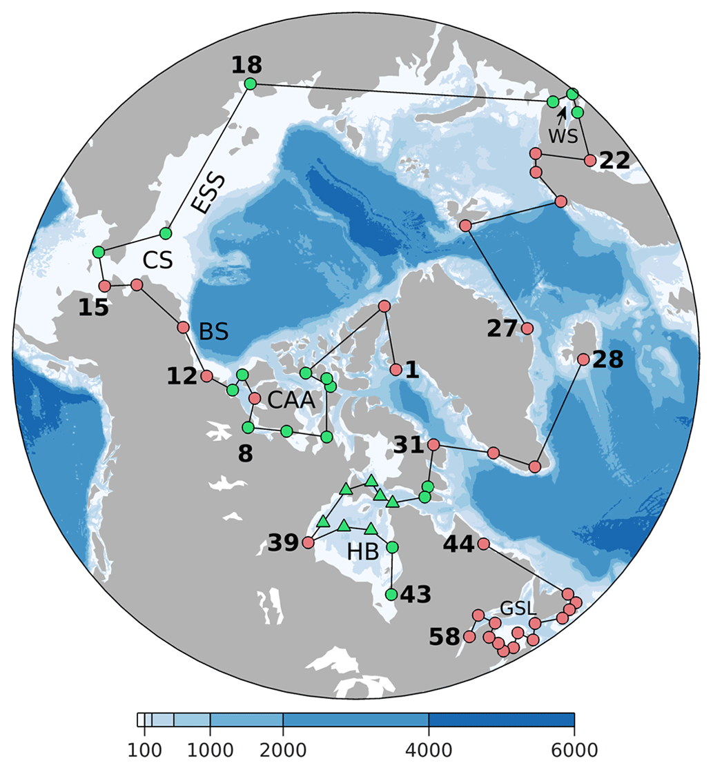
Figure 1 Tide gauges (circles) and in situ moorings (triangles) used in the present study. Red/green symbols indicate that data are available/unavailable during our study period from November 2018 to April 2022 (see Fig. 2 for data availability). The contour map shows bathymetry features in meters. Abbreviations are used for the White Sea (WS), East Siberian Sea (ESS), Chukchi Sea (CS), Beaufort Sea (BS), Canadian Arctic Archipelago (CAA), Hudson Bay (HB), and Gulf of St. Lawrence (GSL). The three subregions, their abbreviations, and stations numbers are as follows: (1) Arctic (Arctic, 1–27), (2) North Atlantic and Hudson Bay (NAHB, 28–43), and (3) northwestern Atlantic (NWA, 44–58).

To understand the underlying physics leading to the seasonal modulation of tides, it is desirable to isolate processes at play. Modeling studies can help separate ice effects from other relevant processes, such as the nonlinear tide–surge interaction (TSI; Bernier and Thompson, 2007) and baroclinicity (Müller et al., 2014). Using a coupled ice–ocean model, St-Laurent et al. (2008), and later Müller et al. (2014), showed that the observed seasonal M₂ modulation in the HB, derived from bottom pressure records, can be largely accounted for by the under-ice friction. As both studies focused on ice processes only, TSI and baroclinicity were not examined. Other studies are based on tide-only models, with under-ice friction expressed as additional bottom friction parameterized solely in terms of ice concentration (e.g., Dunphy et al., 2005; Kleptsova and Pietrzak, 2018) or applied over landfast ice only (Bij de Vaate et al., 2021; Rotermund et al., 2021). These simple methods help produce the ice-induced modulation of tides over particular regions and periods but cannot account for its complex spatial and temporal variability.

For storm surges, ice-induced attenuation has been observed in the Baltic Sea (Lisitzin, 1974) and Beaufort Sea (Henry, 1975). Efforts have been made to include such effects in storm surge modeling. Kowalik (1984) and Danard et al. (1989) applied models that include ice–ocean interactions in the Beaufort and Chukchi seas, but neither one verified the ice effects on surges for winter storm events. Zhang and Leppäranta (1995) applied an ice–ocean model in the Baltic Sea and found that the sea surface slope in ice-covered cases may get down to one-third of the ice-free value. More recently, Joyce et al. (2019) incorporated the ice effects on surges through parameterizations of the wind drag coefficient and showed improvements on the coast of Alaska over particular periods. Kim et al. (2021) adopted the method of Joyce et al. (2019) and showed improvements for simulated peak winter surges at Tuktoyaktuk. However, one particular challenge with such a parameterization is that ice concentration alone cannot fully represent the internal ice stress or the ice strength, which is important for the ice drift response to winds (e.g., Fissel and Tang, 1991; Heil and Hibler, 2002) and the subsequent ice–ocean momentum transfer. The ice strength is usually a function of both ice concentration and ice thickness (e.g., Heil and Hibler, 2002); for example, higher ice concentration and thicker ice can enhance the ice strength and reduce the ice–ocean momentum transfer.

In Canada, sea ice effects on TWL forecasts are a major concern; sea ice is a prominent feature in the Canadian Arctic and Hudson Bay and to a much lesser extent on the east coast of Canada. This process is missing in the recently developed global high-resolution ($\mathrm{1}/\mathrm{12}$^∘) TWL system (Wang et al., 2021, 2022) running operationally at Environment and Climate Change Canada (ECCC). The system is currently under active development, by addressing important physical processes, whilst keeping the system easy to maintain and computationally efficient, so that ensemble forecasts can be performed and made available with sufficient lead time to allow maximum response time for the authorities and the public. Following this principle, we have developed effective and efficient methods to address TWL contributions from tides, storm surges, baroclinicity, and their interactions (Kodaira et al., 2016a, b; Wang et al., 2021, 2022). In the present study, we attempt to further address sea ice effects following the same principle.

As in other operational centers, ECCC has recently developed advanced operational ice–ocean systems with data assimilation and more realistic representations of ice physics and its interaction with the ocean (Smith et al., 2016, 2018; Lemieux et al., 2015, 2016; Roy et al., 2015). These systems are generally not suitable for accurate and timely water level forecast, as their horizontal resolution is too coarse (1/4^∘), their computational cost is not sufficiently low, and/or tides or other processes critical to TWL forecasts are not considered. However, they can offer the information necessary to account for ice effects in higher-resolution, computationally efficient systems optimized to forecast TWLs. In this study, we aim to address the following questions: (1) can we design a new parameterization to include ice effects in a global ocean model for forecasting TWL and improve forecast skill in polar regions? (2) Can we isolate and explain the contribution of dominant physical processes (e.g., under-ice friction, baroclinicity, and nonlinear tide–surge interaction) to the seasonal modulation of tides?

The structure of the paper is as follows. The observations of coastal TWL are described in Sect. 2. The ocean model is introduced in Sect. 3. The new parameterization of ice effects, via the ice–ocean stress, is described in Sect. 4. The experimental design and analysis are presented in Sect. 5. The impact of adding ice effects on the forecast skill and the underlying physics are examined in Sect. 6. The results are summarized and discussed in the final section.

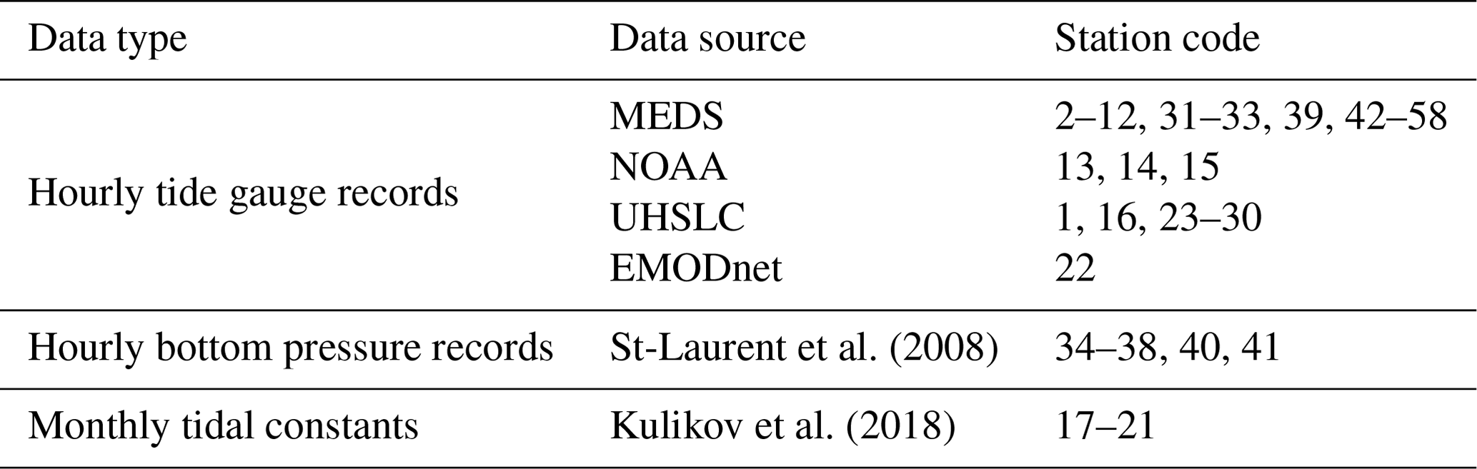
St-Laurent et al. (2008)Kulikov et al. (2018)

Table 1 Summary of water level observations collected from various institutes and publications (see Fig. 1 for station code and Fig. 2 for data availability). Abbreviations are used for Marine Environmental Data Service (MEDS), National Oceanic and Atmospheric Administration (NOAA), University of Hawaii Sea Level Center (UHSLC), and European Marine Observation and Data Network (EMODnet).

2 Observations

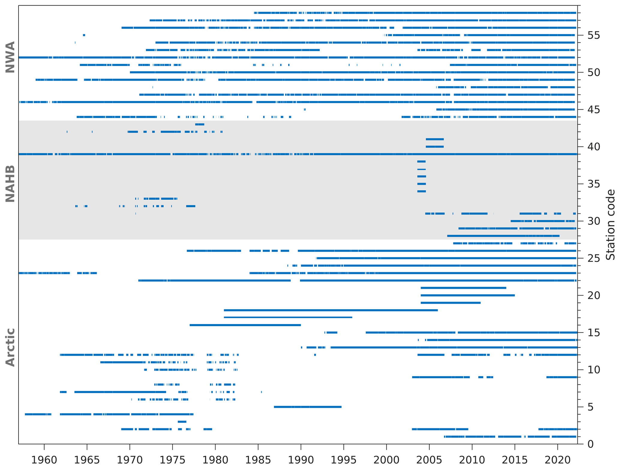
The present study uses 58 stations grouped into three subregions (Fig. 1). Permanent tide gauges (red circles) in the Arctic are very sparse and primarily located around the Beaufort Sea, Chukchi Sea, and northern Norway. In an effort to maximize observations available for verification, we collected data, including tide gauge records, bottom pressure records, and monthly tidal constants from various institutes and publications (Table 1), dating back as early as 1957. Our initial criteria were that stations have records of at least 12 continuous months. More details about data availability, for each station, are given in Fig. 2.

Data quality control was conducted by removing isolated and clustered spikes in TWL records and tidal residuals following careful visual inspection. In addition, the tide gauge record at station 2 before 1969 was not used, as it shows significantly different statistical properties (e.g., variance, seasonal cycle, and datum) than the remaining data. The bottom pressure record at station 40 from August 2003 to August 2004 was discarded, as it has a much coarser temporal resolution than the remainder of the record.

Figure 2 Availability of observed water levels as a function of station code (see Fig. 1) from January 1957 to April 2022.

3 The ocean model

The NEMO modeling framework (Madec, 2008) is used to solve the governing equations (i.e., the momentum equation, continuity equation, and equations for heat and salt transport). They are as follows:

$$\begin{array}{}\text{(1)}& {\displaystyle }\begin{array}{rl}{\displaystyle \frac{\partial {\mathit{u}}_{\mathrm{h}}}{\partial t}}& +\mathit{u}\cdot \mathrm{\nabla }{\mathit{u}}_{\mathrm{h}}+f\times {\mathit{u}}_{\mathrm{h}}=\\ & -{\mathrm{\nabla }}_{\mathrm{h}}\left[{\displaystyle \frac{p_{\mathrm{a}}}{{\mathit{\rho }}_{\mathrm{0}}}}+g(\mathrm{1}-{\mathit{\alpha }}_{\mathrm{s}})\mathit{\eta }-g{\mathit{\eta }}_{\mathrm{A}}+g\underset{\mathrm{z}}{\overset{\mathrm{0}}{\int }}{\displaystyle \frac{\mathit{\rho }-{\mathit{\rho }}_{\mathrm{0}}}{{\mathit{\rho }}_{\mathrm{0}}}}\mathrm{d}z\right]\\ & +A_{\mathrm{h}}{\mathrm{\nabla }}_{\mathrm{h}}^{\mathrm{2}}{\mathit{u}}_{\mathrm{h}}+{\displaystyle \frac{\partial }{\partial z}}\left(A_{\mathrm{z}}{\displaystyle \frac{\partial {\mathit{u}}_{\mathrm{h}}}{\partial z}}\right)-\mathit{\lambda }\left(\mathit{x}\right)\langle {\stackrel{\mathrm{‾}}{\mathit{u}}}_h-{\stackrel{\mathrm{‾}}{\mathit{u}}}_{\text{obs}}\rangle ,\end{array}\text{(2)}& {\displaystyle }\mathrm{\nabla }\cdot \mathit{u}=\mathrm{0},\text{(3)}& {\displaystyle \frac{\partial T}{\partial t}}+\mathrm{\nabla }\cdot \left(T\mathit{u}\right)=K_{\mathrm{h}}{\mathrm{\nabla }}_{\mathrm{h}}^{\mathrm{2}}T+{\displaystyle \frac{\partial }{\partial z}}\left(K_{\mathrm{z}}{\displaystyle \frac{\partial T}{\partial z}}\right)-r(T-T_{\mathrm{f}}),\text{(4)}& {\displaystyle \frac{\partial S}{\partial t}}+\mathrm{\nabla }\cdot \left(S\mathit{u}\right)=K_{\mathrm{h}}{\mathrm{\nabla }}_{\mathrm{h}}^{\mathrm{2}}S+{\displaystyle \frac{\partial }{\partial z}}\left(K_{\mathrm{z}}{\displaystyle \frac{\partial S}{\partial z}}\right)-r(S-S_{\mathrm{f}}),\end{array}$$

where u_h represents the horizontal velocity vector (u,v), u denotes the complete velocity vector in three dimensions ($u,v,w$), f is the Coriolis parameter, p_a denotes atmospheric pressure at the sea level, ρ₀ denotes the reference density (1025 kg m⁻³), η denotes the sea surface height, and η_A represents the gravitational tidal potential. The depth-dependent coefficient α_s is used to parameterize the impact of self-attraction and loading (Stepanov and Hughes, 2004). The lateral eddy viscosity and diffusivity coefficients are set to constant (A_h = 100 m² s⁻¹ and K_h = 10 m² s⁻¹), and the vertical eddy viscosity and diffusivity coefficients (A_z and K_z) are determined using the turbulent kinetic energy scheme introduced in Gaspar et al. (1990).

In Eq. (1), the last term on the right-hand side represents the tidal nudging technique introduced in Wang et al. (2021). It nudges the model's depth-averaged current ${\stackrel{\mathrm{‾}}{\mathit{u}}}_h$ towards the observed current ${\stackrel{\mathrm{‾}}{\mathit{u}}}_{\text{obs}}$ calculated using the tidal amplitude and phase of eight major tidal constituents (M₂, S₂, N₂, K₂, O₁, K₁, P₁, and Q₁) provided by TPXO8 (Egbert and Erofeeva, 2002). The angle brackets indicate that the nudging is filtered temporally to isolate the variability in tidal frequency bands. The strength of the nudging is determined by a spatially varying coefficient λ(x). South of 66^∘ N its global distribution is given by Wang et al. (2021). North of 66^∘ N, we set λ(x) to zero because the nudging would dampen the ice-induced seasonal modulation of tides. Recall that TPXO8 does not take ice effects into account, and so nudging is not desired when ice effects are considered.

In Eqs. (3) and (4), the last terms on the right-hand side correspond to the nudging of the model's temperature and salinity (T and S), towards operational forecasts (T_f and S_f) provided by a coarser-resolution ($\mathrm{1}/\mathrm{4}$^∘) data-assimilative system – the Global Ice Ocean Prediction System (GIOPS; Smith et al., 2016, 2018). The strength of the nudging is controlled by a spatially uniform coefficient r. We set r = 0.2 d⁻¹, and this adds the high-quality, low-frequency variability (with periods exceeding about 15 d) provided by the $\mathrm{1}/\mathrm{4}$^∘ model to our TWL model, while allowing high-frequency variability to evolve freely (Wang et al., 2022).

At the surface, the boundary condition for Eq. (1) is given by

$$\begin{array}{}\text{(5)}& \begin{array}{rl}{A}_{\mathrm{z}}{\left.{\displaystyle \frac{\partial {\mathit{u}}_{\mathrm{h}}}{\partial z}}\right|}_{z=\mathrm{0}}& ={\displaystyle \frac{{\mathit{\tau }}_{\mathrm{s}}}{{\mathit{\rho }}_{\mathrm{0}}}},\\ {\mathit{\tau }}_{\mathrm{s}}& ={\mathit{\tau }}_{\text{ao}}={\mathit{\rho }}_{\mathrm{a}}{C}_{\text{ao}}\left|{\mathit{u}}_{\mathrm{10}}\right|{\mathit{u}}_{\mathrm{10}}(\mathit{\alpha }=\mathrm{0}),\end{array}\end{array}$$

where ρ_a denotes the air density, and u₁₀ is the wind velocity at 10 m height. In the absence of sea ice (i.e., ice concentration α equals zero), the surface stress τ_s equals the air–ocean stress τ_ao. The air–ocean drag coefficient C_ao equals 1.2 × 10⁻³ for $\left|{\mathit{u}}_{\mathrm{10}}\right|<$ 8 m s⁻¹ and then increases linearly with $\left|{\mathit{u}}_{\mathrm{10}}\right|$, with a slope of 0.065 × 10⁻³ for every 1 m s⁻¹ increase in $\left|{\mathit{u}}_{\mathrm{10}}\right|$ (Bernier and Thompson, 2007). Hourly fields of u₁₀ and p_a were obtained from the assimilation component of ECCC's operational Global Deterministic Prediction System (GDPS; Buehner et al., 2015), with a grid spacing of roughly 15 km.

At the bottom, the boundary condition for Eq. (1) is

$$\begin{array}{}\text{(6)}& A_{\mathrm{z}}{\left.{\displaystyle \frac{\partial {\mathit{u}}_h}{\partial z}}\right|}_{z=-H}={\displaystyle \frac{{\mathit{\tau }}_{\mathrm{b}}}{{\mathit{\rho }}_{\mathrm{0}}}},{\mathit{\tau }}_{\mathrm{b}}={\mathit{\rho }}_{\mathrm{0}}{C}_{\text{db}}\left|{\mathit{u}}_{\mathrm{b}}\right|{\mathit{u}}_{\mathrm{b}},\end{array}$$

where τ_b refers to the bottom stress, u_b denotes the current velocity at the bottom, and C_db is the bottom drag coefficient, which is set equal to 2.5 × 10⁻³.

The extended version of a tripolar ORCA grid (eORCA12) is used as the model grid. It covers the Antarctic ice shelves and has a horizontal grid spacing of $\mathrm{1}/\mathrm{12}$^∘. The bathymetry is obtained from GEBCO_2014 (Weatherall et al., 2015), with local adjustments made in the HB and on the Labrador and Newfoundland shelves, based on bathymetric data provided by Florent H. Lyard (personal communication). Following Wang et al. (2022), the vertical grid is nine z levels, which is able to capture baroclinic variability via T and S nudging, whilst maintaining low computational cost. Partial steps are employed for the bottom layer to achieve a more accurate representation of the bathymetry. Mode splitting was used, with time steps of 240 and 6 s for the internal and external modes, respectively.

4 Surface stress in the presence of sea ice

In this section, we describe the surface stress τ_s in the presence of sea ice. We review parameterizations or models previously developed and introduce a new, cost-efficient, method for its parameterization in TWL systems.

In the presence of sea ice, τ_s is generally approximated by a combination of the air–ocean stress τ_ao (see Eq. 5) and the ice–ocean stress τ_io weighted by the ice concentration α as follows:

$$\begin{array}{}\text{(7)}& {\mathit{\tau }}_{\mathrm{s}}=(\mathrm{1}-\mathit{\alpha }){\mathit{\tau }}_{\text{ao}}+\mathit{\alpha }{\mathit{\tau }}_{\text{io}}.\end{array}$$

τ_io can be parameterized by a quadratic drag law in terms of the relative velocity between ice and surface currents (u_ice−u_surf) as follows:

$$\begin{array}{}\text{(8)}& {\mathit{\tau }}_{\text{io}}={\mathit{\rho }}_{\mathrm{0}}{C}_{\text{io}}|{\mathit{u}}_{\text{ice}}-{\mathit{u}}_{\text{surf}}|({\mathit{u}}_{\text{ice}}-{\mathit{u}}_{\text{surf}}),\end{array}$$

where C_io is the ice–ocean drag coefficient.

To address τ_io, there are several options with different levels of complexity. The most complex option is to couple the ocean model with a sophisticated ice model that simulates ice thermodynamics, dynamics, transport, and ridging (Hunke et al., 2010). Unfortunately, such an option is not suitable for relatively high-resolution systems built with computational efficiency in mind. A simpler option is to solve the ice momentum equation with prescribed ice concentration and ice thickness. However, the major time-consuming part in most modern ice modeling, the sub-cycling of the standard elastic–viscous–plastic solver for ice dynamics (Hunke and Dukowicz, 1997), is still required. In addition, the simplified coupling neglects mass transport, and so it has deleterious effects known as “artificial inertial resonance” in the presence of both tidal and wind forcing (Hibler et al., 2006). Another option is to take u_ice−u_surf directly from an external ice–ocean model, which requires only a negligible additional computational cost. The main issue with this option is the potentially large inconsistency in predicted tides between the TWL and external ice–ocean models. These differences can have various sources such as model resolution, bottom topography, open boundary conditions, and parameterization of dissipation. In the following section, we propose and evaluate a new approach to address these inconsistencies.

4.1 Mapping ice effects on currents

To address the inconsistency issue in tides associated with the use of an external ice–ocean model to define the ice–ocean stress while maintaining computational efficiency, we decompose the relative velocity into a tidal component (denoted with the superscript T) and a residual/surge component (superscript S) as follows:

$$\begin{array}{}\text{(9)}& {\mathit{u}}_{\text{ice}}-{\mathit{u}}_{\text{surf}}=\left({\mathit{u}}_{\text{ice}}^{\text{T}}-{\mathit{u}}_{\text{surf}}^{\text{T}}\right)+\left({\mathit{u}}_{\text{ice}}^{\mathrm{S}}-{\mathit{u}}_{\text{surf}}^{\mathrm{S}}\right).\end{array}$$

As ${\mathit{u}}_{\text{ice}}^{\text{T}}$ is mainly forced by ${\mathit{u}}_{\text{surf}}^{\text{T}}$, we introduce a transfer function, such that

$$\begin{array}{}\text{(10)}& {\mathit{u}}_{\text{ice}}^{\text{T}}\approx a^{\mathrm{T}}\left(\mathit{x}\right)\mathbf{R}\left(\mathit{\phi }\right(\mathit{x}\left)\right){\mathit{u}}_{\text{surf}}^{\text{T}},\end{array}$$

where

$$\begin{array}{}\text{(11)}& \mathbf{R}\left(\mathit{\phi }\right(\mathit{x}\left)\right)=\left[\begin{array}{lr}\cos \mathit{\phi }\left(\mathit{x}\right)& -\sin \mathit{\phi }\left(\mathit{x}\right)\\ \sin \mathit{\phi }\left(\mathit{x}\right)& \cos \mathit{\phi }\left(\mathit{x}\right)\end{array}\right],\end{array}$$

and the spatially varying scale factor a^T and the rotation angle φ can be inferred from ${\mathit{u}}_{\text{ice}}^{\mathrm{T}\ast }$ and ${\mathit{u}}_{\text{surf}}^{\mathrm{T}\ast }$ provided by external ice–ocean models (the asterisk ^∗ denotes quantities from external models). Specifically, a^T and φ are derived by scaling and rotating the ice and ocean tidal ellipses so that their semi-major axes are equal. The tidal relative velocity is thus written as

$$\begin{array}{}\text{(12)}& {\mathit{u}}_{\text{ice}}^{\text{T}}-{\mathit{u}}_{\text{surf}}^{\text{T}}=\left[a^{\mathrm{T}}\left(\mathit{x}\right)\mathbf{R}\left(\mathit{\phi }\right(\mathit{x}\left)\right)-\mathbf{I}\right]{\mathit{u}}_{\text{surf}}^{\text{T}},\end{array}$$

where I is the identity matrix.

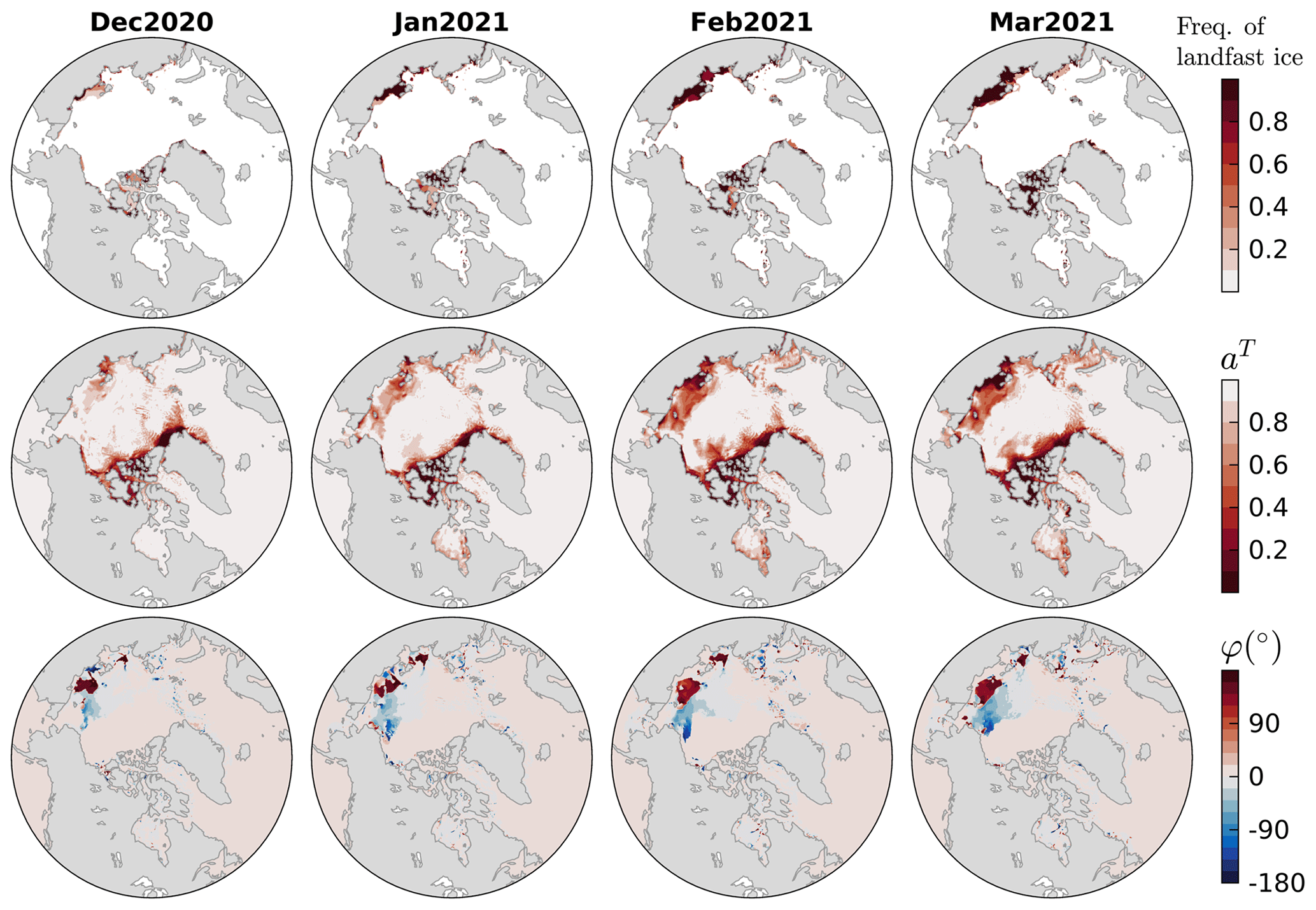
Figure 3 Top panels show the observed frequency of the landfast ice occurrence for December 2020 to March 2021, calculated based on the weekly fast ice extent provided by the U.S. National Ice Center (2020). Middle and bottom panels show the derived monthly a^T and φ for the M₂ tide for the same period. Note that for areas with very weak ${\mathit{u}}_{\text{ice}}^{\mathrm{T}\ast }$ (major axis velocity magnitude less than 5 × 10⁻³ m s⁻¹ in this study), φ is irrelevant, its estimation is also not reliable, and so it is set to 0.

Unlike periodic tides, storm surges are sporadic and occur on a local scale driven by the atmospheric forcing. Applying a transfer function to ${\mathit{u}}_{\text{surf}}^{\mathrm{S}}$, similar to Eq. (10), is not feasible, since ${\mathit{u}}_{\text{surf}}^{\mathrm{S}}$ is forced by ${\mathit{u}}_{\text{ice}}^{\mathrm{S}}$. Instead, we expect that the inconsistency in surges between our model and the external ice–ocean model is acceptable, given that their atmospheric forcings are similar. The residual relative velocity can thus be taken directly from the external model. Since the tidal and residual relative velocities are calculated based on surface currents coming from the TWL and external models, respectively, their valid surface levels could be different. To be consistent, an empirical scale factor, a^S, can be used to adjust the residual relative velocities to the surface levels of the TWL model as follows:

$$\begin{array}{}\text{(13)}& {\mathit{u}}_{\text{ice}}^{\mathrm{S}}-{\mathit{u}}_{\text{surf}}^{\mathrm{S}}=a^{\mathrm{S}}\left({\mathit{u}}_{\text{ice}}^{\mathrm{S}\ast }-{\mathit{u}}_{\text{surf}}^{\mathrm{S}\ast }\right).\end{array}$$

For example, if the surface level in the external model is shallower than the TWL model, then ${\mathit{u}}_{\text{surf}}^{\mathrm{S}\ast }$ will be stronger than ${\mathit{u}}_{\text{surf}}^{\mathrm{S}}$, and a^S should be larger than unity. In practice, a^S can be tuned to best reproduce the observed residual water level in the presence of ice.

Finally, the total relative velocity is

$$\begin{array}{}\text{(14)}& \begin{array}{rl}{\mathit{u}}_{\text{ice}}-{\mathit{u}}_{\text{surf}}=& \left[a^{\mathrm{T}}\left(\mathit{x}\right)\mathbf{R}\left(\mathit{\phi }\right(\mathit{x}\left)\right)-\mathbf{I}\right]{\mathit{u}}_{\text{surf}}^{\text{T}}\\ & +a^{\mathrm{S}}\left({\mathit{u}}_{\text{ice}}^{\mathrm{S}\ast }-{\mathit{u}}_{\text{surf}}^{\mathrm{S}\ast }\right).\end{array}\end{array}$$

In practice, ${\mathit{u}}_{\text{surf}}^{\text{T}}=\langle {\mathit{u}}_{\text{surf}}\rangle$ can be obtained using an efficient online tidal filter (Wang et al., 2021) denoted by the angle brackets. Note that the same filter is also used for the tidal nudging shown in the last term on the right-hand side of Eq. (1).

4.2 Ice–ocean stress

Gridded fields of hourly ice concentration (α), ice velocity (${\mathit{u}}_{\text{ice}}^{\mathrm{T}\ast }$; ${\mathit{u}}_{\text{ice}}^{\mathrm{S}\ast }$), and surface current (${\mathit{u}}_{\text{surf}}^{\mathrm{T}\ast }$; ${\mathit{u}}_{\text{surf}}^{\mathrm{S}\ast }$) were obtained from the assimilation component of GIOPS (Smith et al., 2016, 2018) developed and run operationally at ECCC. In GIOPS, the CICE-based (Hunke et al., 2010) ice component has 10 categories of ice thickness, and the NEMO-based ocean component has 50 vertical levels and a horizontal resolution of $\mathrm{1}/\mathrm{4}$^∘. The initialization of GIOPS involves using analyses created by Mercator Océan's System d'Assimilation Mercator, version 2 (SAM2; Tranchant et al., 2008). Further information regarding the initialization procedures can be found in Smith et al. (2018). We note that although GIOPS is a global system, its model grid has a southern limit at about 77^∘ S, which excludes ice cavities in the Ross Sea and Weddell Sea. In the present study, we thus focus on ice-infested waters of the Northern Hemisphere.

As in many global ice–ocean systems, the operational GIOPS does not include tides. To obtain ${\mathit{u}}_{\text{ice}}^{\mathrm{T}\ast }$ and ${\mathit{u}}_{\text{surf}}^{\mathrm{T}\ast }$, we reran GIOPS by activating the astronomical tidal potential forcing. In the present study, the transfer function is updated monthly, which is sufficient to capture its seasonality. We focus on four major tidal constituents (M₂, S₂, K₁, and O₁) in GIOPS, as they can be adequately resolved with monthly harmonic analyses.

Figure 3 (middle panels) illustrates the monthly estimates of a^T for M₂ from December 2020 to March 2021. Note that a^T captures the mobility of sea ice, with landfast for a^T=0, non-free drift for $\mathrm{0}<a^{\mathrm{T}}<\mathrm{1}$, and free drift for a^T=1. In theory, only landfast ice and non-free drift ice exert friction on the underlying ocean flow. Regions of a^T→0 are seen along the Arctic coast, in parts of the Canadian Arctic Archipelago (CAA), and the East Siberian Sea (ESS). Identified regions are in reasonable agreement with observed landfast ice occurrences (top panels). Non-free drift ice is found further away from the coast in the Arctic and HB, and in particular, it covers broad areas of the ESS and CS. We note that not all the identified landfast or non-free drift ice are relevant for the seasonality of tides. We return to this point later (see the end of Sect. 6.2.2). The rotation angle φ is only relevant for drift ice. Its main impact is found in the ESS and CS, where the tidal ice and ocean velocity vectors can be nearly 180^∘ out of phase (bottom panels of Fig. 3), effectively enhancing the under-ice friction. Elsewhere, the absolute value of φ is relatively small (within 20^∘), which has minimal effects on the calculation of the under-ice friction.

Results for the other three constituents are roughly similar to M₂ (not shown), although over some regions (e.g., ESS and CS) K₁ and O₁ are too weak to derive reliable estimates. This similarity between constituents indicates that the transfer function, or the response of sea ice relative to tidal current, is largely determined by ice characteristics. Thus each monthly transfer function for M₂ was applied to other constituents in the present study. We note that the main advantage of this new approach is that it is not sensitive to differences in predicted tides between the ice–ocean and TWL models, as the mapping of ice effects is achieved via a transfer function. Therefore, in theory, the approach can be used with any ice–ocean systems, regardless of the model skill in tides – as long as they are realistic.

4.3 Ice–ocean drag coefficient

The parameterization of the ice–ocean drag coefficient C_io is a complex issue, as C_io depends on various ice characteristics, such as surface roughness, floe size, ridge height, and keel depth (Lu et al., 2011; Tsamados et al., 2014). Instead, constant values are commonly used and determined by matching model predictions with observations (e.g., St-Laurent et al., 2008; Rotermund et al., 2021). Typical measured C_io values range from 1.05 × 10⁻³ to 4.70 × 10⁻² in field investigations (see Table 1 in Lu et al., 2011). GIOPS has 50 vertical levels, and its C_io was set to 2.32 × 10⁻², based on a log layer assumption, using its first-layer currents at 0.5 m and an undersurface sea ice roughness length scale of 0.030 m (Roy et al., 2015). In the TWL system, only nine vertical levels are used (Wang et al., 2022), and so our first-layer currents are valid at 7.5 m. The C_io value for our model is thus expected to be smaller than that used by GIOPS, but the log layer assumption used in GIOPS is not suitable for our first layer. Based on sensitivity tests, we set C_io to 1.00 × 10⁻², which produces reasonable agreement between observed and predicted seasonal M₂ modulations.

The empirical scale factor for residual relative velocity, a^S in Eq. (14), was tuned to 1.64, which produces reasonable agreement between observed and predicted residuals. To offer an alternative interpretation of this value, we note that the resulting drag coefficient (a^S)²C_io for the residual stress based on ${\mathit{u}}_{\text{ice}}^{\mathrm{S}\ast }-{\mathit{u}}_{\text{surf}}^{\mathrm{S}\ast }$ is 2.69 × 10⁻², indicating a slightly higher roughness length scale of about 0.036 m, compared to 0.030 m used in GIOPS (Roy et al., 2015), which is well within the range given in the literature. As an example, McPhee (2008) provides a mean value of 0.049 m, with a standard deviation ranging between 0.016 and 0.146 m, based on estimates for a typical multiyear sea ice floe.

5 Experimental design and analysis

Two basic runs, Run_AO and Run_AIO, were conducted to examine the impact of adding ice effects on predicted water levels. In Run_AO, ice effects are not considered, and τ_s equals τ_ao (see Eq. 5). In Run_AIO, τ_s is computed as the combination of τ_ao and τ_io (see Eq. 7). In order to quantify the contribution of individual physical processes on the seasonality of tide, four process-oriented runs were also conducted by gradually removing the relevant processes from Run_AIO, including the baroclinic effects (by using constant T and S; Run1), TSI due to τ_io (Run2), TSI due to τ_b (Run3), under-ice friction (by setting ${\mathit{u}}_{\text{ice}}^{\text{T}}-{\mathit{u}}_{\text{surf}}^{\text{T}}$ to zero; Run4). Specifically, for Run2, TSI due to τ_io was removed by setting ${\mathit{\tau }}_{\text{io}}={\mathit{\rho }}_{\mathrm{0}}{C}_{\text{io}}\left(\right|{\mathit{u}}_{\text{io}}^{\text{T}}|{\mathit{u}}_{\text{io}}^{\text{T}}+|{\mathit{u}}_{\text{io}}^{\mathrm{S}}\left|{\mathit{u}}_{\text{io}}^{\mathrm{S}}\right)$, where ${\mathit{u}}_{\text{io}}^{\text{T}}$ and ${\mathit{u}}_{\text{io}}^{\mathrm{S}}$ are, respectively, the tidal and residual relative ice–ocean velocities given by Eqs. (12) and (13). For Run3, TSI due to τ_b was removed by setting ${\mathit{\tau }}_{\mathrm{b}}={\mathit{\rho }}_{\mathrm{0}}{C}_{\text{db}}\left(\right|{\mathit{u}}_{\mathrm{b}}^{\text{T}}|{\mathit{u}}_{\mathrm{b}}^{\text{T}}+|{\mathit{u}}_{\mathrm{b}}^{\mathrm{S}}\left|{\mathit{u}}_{\mathrm{b}}^{\mathrm{S}}\right)$, where ${\mathit{u}}_b^{\text{T}}$ and ${\mathit{u}}_b^{\mathrm{S}}$ are isolated using the online tidal filter of Wang et al. (2021), with ${\mathit{u}}_b^{\text{T}}=\langle {\mathit{u}}_{\mathrm{b}}\rangle$; ${\mathit{u}}_b^{\mathrm{S}}={\mathit{u}}_{\mathrm{b}}-\langle {\mathit{u}}_{\mathrm{b}}\rangle$.

Table 2 Design of the model experiments.

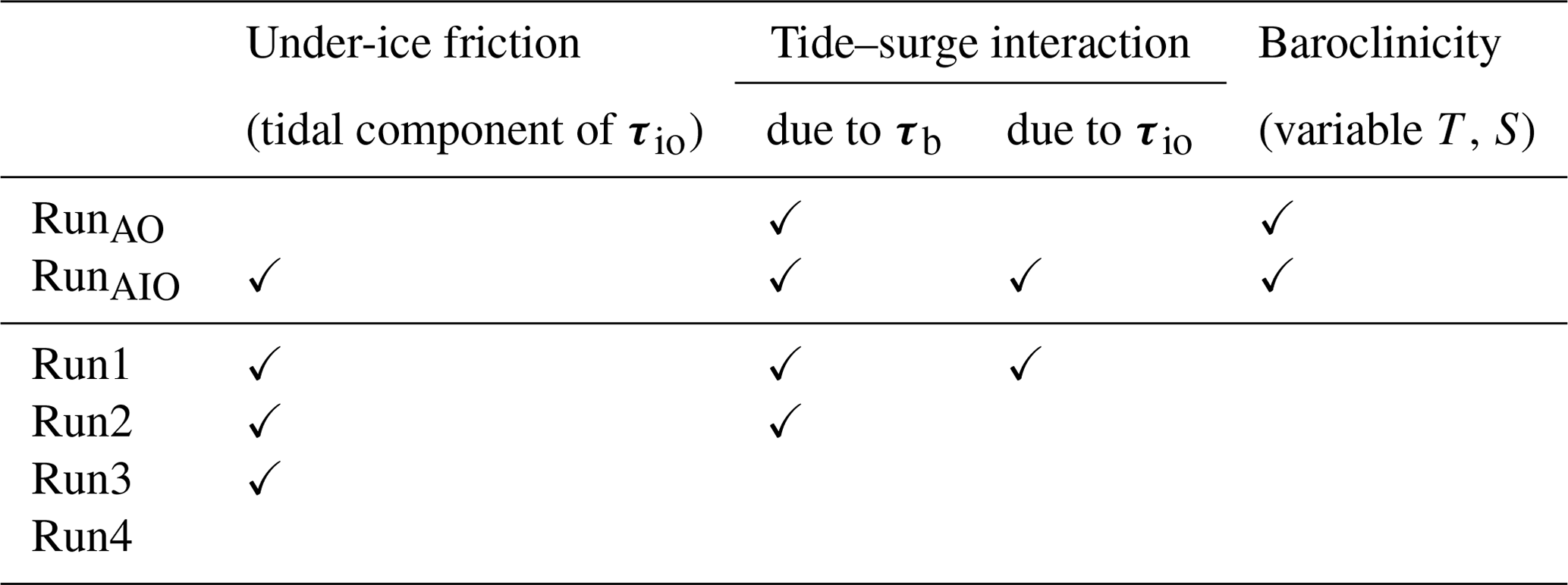
The six runs are summarized in Table 2. Note that we chose to remove processes gradually instead of the more traditional removal of a process at a time because it is not possible to completely isolate the under-ice friction which is a prerequisite for the TSI due to τ_io. Sensitivity studies (not shown) confirm that the impact of the combined removal approach on other processes that can be isolated (i.e., the TSI due to τ_io and τ_b) is negligible. Each model run starts on 21 September 2018 and finishes on 30 April 2022. The first 40 d of a run are discarded to allow for model spin-up, which is mainly determined by the spin-up of the tidal nudging (Wang et al., 2021).

We use the root mean square error (RMSE) to evaluate the model performance for individual stations. To facilitate the comparison with different scales, we also compute the root mean square (rms) of the observations. Both metrics were calculated for TWL, tides, and tidal residuals at each station. Tides were reconstructed based on the eight major tidal constituents used in this study (see Sect. 3), using the T_TIDE package of Pawlowicz et al. (2002).

Monthly harmonic analyses of observed and predicted TWL were conducted to examine the ice-induced seasonality of tides. It is noted that for diurnal tides, there is substantial variability in the standard monthly analysis, possibly due in part to the contamination from non-tidal energy (Cartwright and Amin, 1986). To minimize such an effect and focus on the seasonal variability, we conducted another set of monthly analyses, using a sliding window of 90 d to obtain the estimates for diurnal tides only. The unresolvable constituent K₂ (P₁) was inferred from S₂ (K₁), and the inference parameters including amplitude ratios and phase differences were taken from the yearly analysis. Nodal corrections were performed. Estimates for stations with a signal-to-noise ratio (SNR; see Pawlowicz et al., 2002, for details) lower than 2 are not used.

For each year, we calculate the normalized amplitude anomaly ($\mathrm{\Delta }{\stackrel{\mathrm{̃}}{A}}_i$) and phase anomaly (Δϕ_i) relative to their corresponding values in September (A_Sept, ϕ_Sept), when sea ice has the minimum cover in the Arctic. Thus,

$$\begin{array}{}\text{(15)}& {\displaystyle }& {\displaystyle }\mathrm{\Delta }{\stackrel{\mathrm{̃}}{A}}_i={\displaystyle \frac{A_i-A_{\text{Sept}}}{A_{\text{Sept}}}}\text{(16)}& {\displaystyle }& {\displaystyle }\mathrm{\Delta }{\mathit{\varphi }}_i={\mathit{\varphi }}_i-{\mathit{\varphi }}_{\text{Sept}},\end{array}$$

where the subscript i denotes a particular month. The ice-induced maximum modulation occurs in March ($\mathrm{\Delta }{\stackrel{\mathrm{̃}}{A}}_{\text{Mar}}$; ϕ_Mar) when sea ice reaches its maximum. We note that the seasonality of tides can be caused by a variety of mechanisms, including astronomical motions, frictional/advective interactions, and climate processes (e.g., baroclinicity, sea ice, and river discharge; Ray, 2022). In the main text, we focus on the seasonality of the dominant M₂ constituent, which has negligible astronomical contribution. Other minor constituents, including S₂, K₁, and O₁, are briefly discussed in the Supplement.

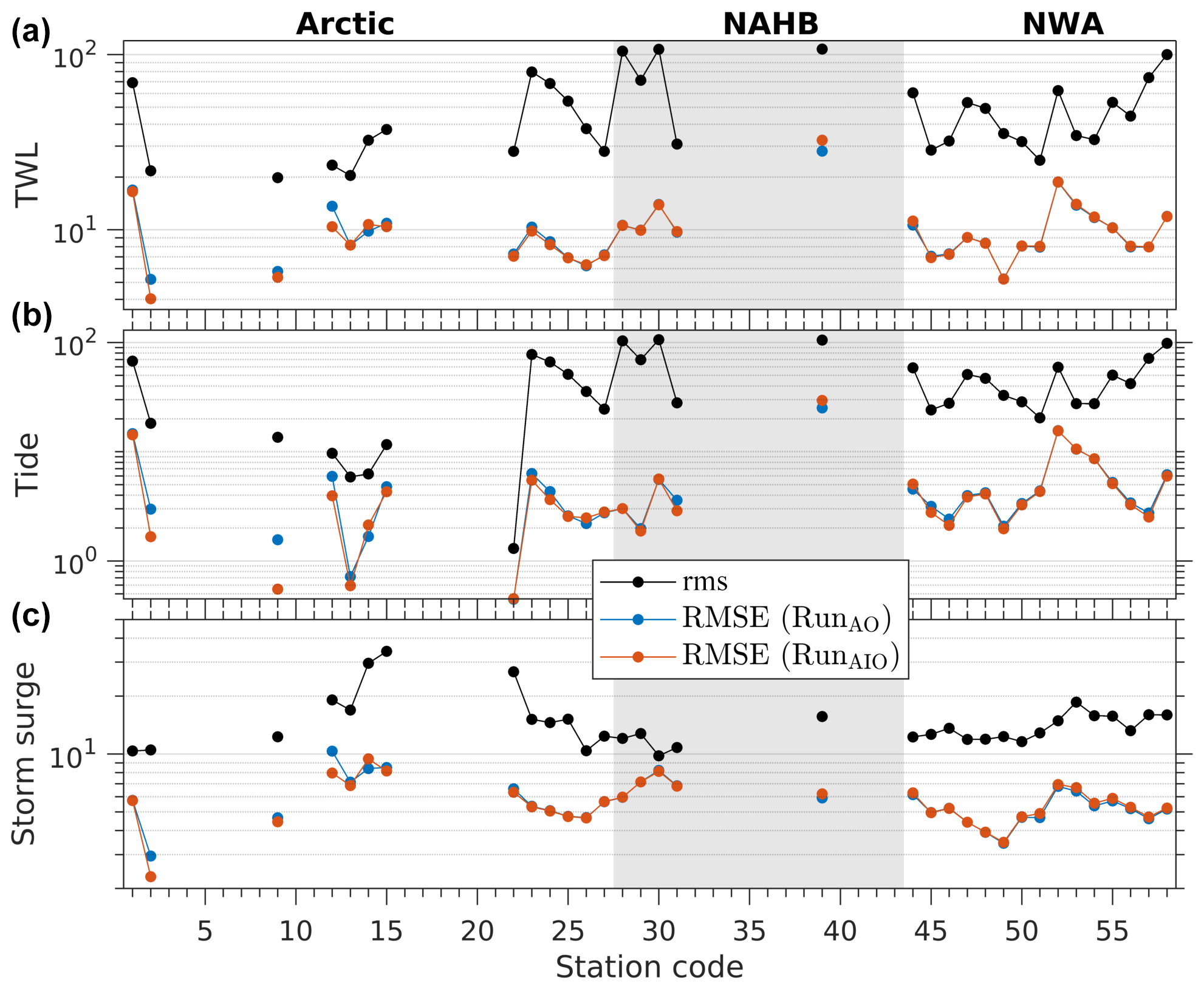
Figure 4 The rms of observations (black) and RMSE for Run_AO (blue) and Run_AIO (red) for TWL (a), tides (b), and storm surges (c). All rms and RMSE values are in centimeters. Note that the missing stations are those for which only historical observations are available, i.e., data do not overlap with the study period.

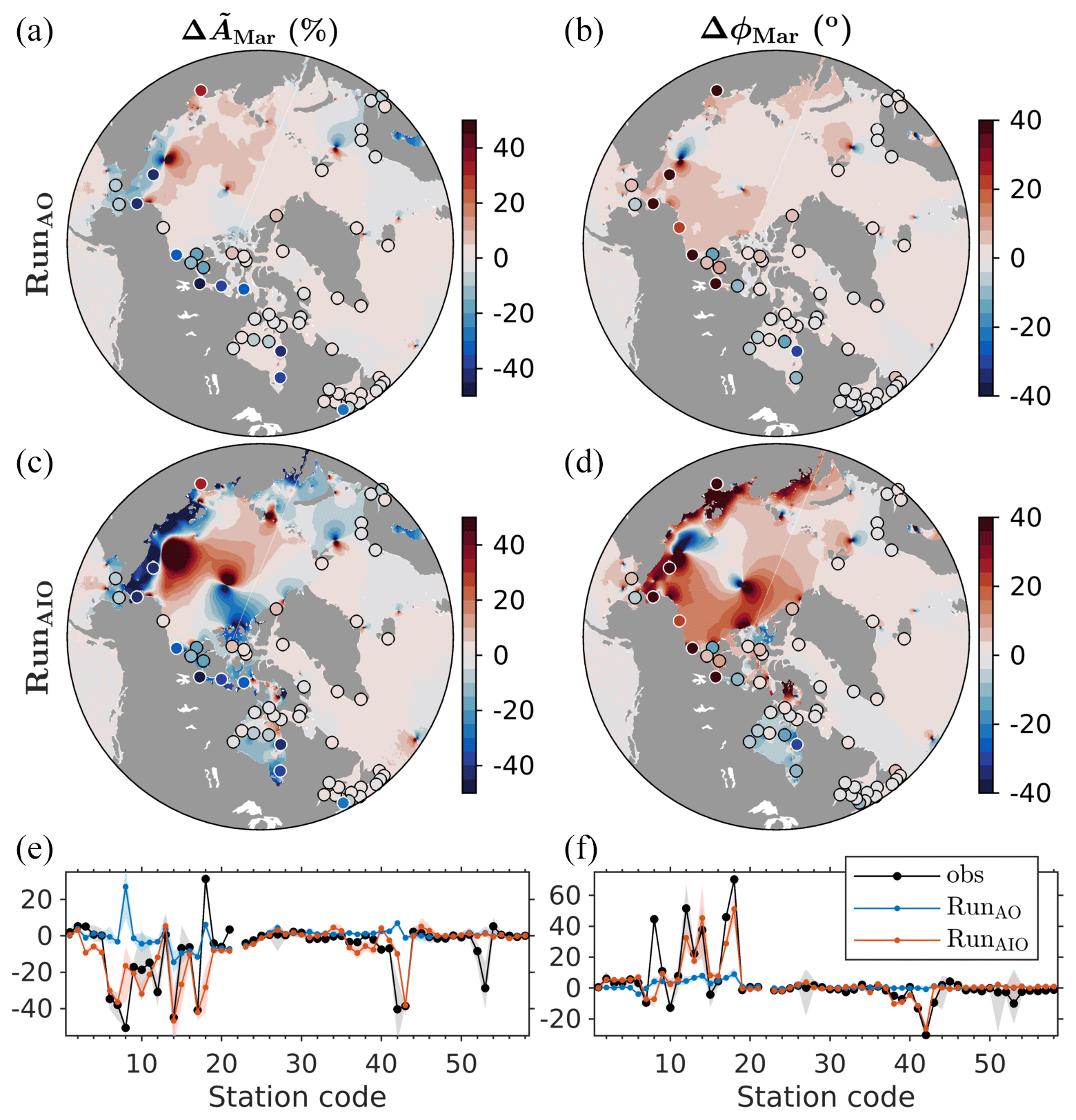
Figure 5 Modulation of the M₂ amplitude ($\mathrm{\Delta }{\stackrel{\mathrm{̃}}{A}}_{\text{Mar}}$; panels a, c, and e) and phase (Δϕ_Mar; panels b, d, and f) in March relative to September. The contour map shows results predicted by Run_AO (a, b) and Run_AIO (c, d) averaged over 2019–2021. Filled circles show results taken from available observations during 1957–2021. (e, f) Comparison between observation and prediction as a function of station code (Fig. 1). Shaded areas indicate the 10th–90th percentile range. Only stations with a SNR greater than 2 are plotted.

6 Results

6.1 Total water level

We first compare the model skill for Run_AO and Run_AIO in predicting TWL in terms of RMSE at 34 permanent tide gauges (Fig. 4a). Improvements from the addition of ice effects are seen in the Arctic, most particularly in the Canadian Arctic (stations 2, 9, and 12). The reductions in RMSE are relatively small (i.e., 1.0–3.3 cm). This is expected, considering that sea ice matters mostly in winter and, in particular, during winter storms which are relatively rare in parts of the Arctic. For example, over the four ice seasons of the study period, there are only two storms at station 2 and no storms at station 9, both of which are located in the CAA. We note, however, that the impact on peak water levels can be large (up to 1.0 m; see Sect. 6.3). The impact at stations in the northern North Atlantic (28–31) and Gulf of St. Lawrence (44–58) is negligible, indicating that the predicted ice is mostly in free drift over these regions. A slight increase in RMSE value of about 4.0 cm is noted at Churchill (station 39) in the HB. This is largely due to the existing bias in the predicted tides under ice-free conditions, thus adding the ice-induced modulation increases the bias in the ice season (Fig. 4b). However, we note that observations at Churchill have possible quality or drift issues, as observed tides have undergone large changes since 1998 (Ray, 2016). Finally, we note that this evaluation is limited to permanent gauges which are very sparse in the Arctic and HB. Next, we focus on the ice effects on the seasonality of tides at all available stations and storm surges during large storm events.

6.2 Tides

6.2.1 Seasonal variability

Figure 5 shows the M₂ modulation in March relative to September ($\mathrm{\Delta }{\stackrel{\mathrm{̃}}{A}}_{\text{Mar}}$, Δϕ_Mar). The ice effects on tides can be understood as a combination of two processes, namely (1) direct frictional effects that result in amplitude reductions (i.e., negative $\mathrm{\Delta }{\stackrel{\mathrm{̃}}{A}}_{\text{Mar}}$) and phase delays (i.e., positive Δϕ_Mar) and (2) indirect effects through the amphidrome shift that leads to both positive and negative changes in amplitude and phase. Comparison of predictions given by Run_AO and Run_AIO (Fig. 5a–d) reveals large ice-induced modulations in the Arctic and HB, with the largest modulations occurring around amphidromic points. Adding ice effects generally reduces the amplitudes at the coast (Fig. 5c), while the opposite also occurs due to the amphidrome shift. Adding ice effects also leads to phase delays in most of the Arctic and the CAA and phase advances in parts of the CAA and most of the HB (Fig. 5d) due to contributions from both the direct and indirect effects of friction. We return to the point regarding the amphidrome shift later (see Sect. 6.2.2). Figure 5a and b also reveal non-negligible M₂ modulations in Run_AO, indicating that nonlinear TSI and/or baroclinicity also contribute to seasonal variability (see Sect. 6.2.3 for details).

Observations (filled circles) are also plotted on top of predictions in Fig. 5a–d. Their comparison is further plotted as function of station code in the bottom panel. Adding ice effects significantly improves the model skill in predicting $\mathrm{\Delta }{\stackrel{\mathrm{̃}}{A}}_{\text{Mar}}$ (up to 40 %) and Δϕ_Mar (up to 50^∘) at most stations in the Arctic and HB. In the Arctic, improvements are also found for other smaller constituents (S₂, K₁, and O₁; see the Supplement for additional details). For M₂, one exception is station 18, where observations show an anomalous positive $\mathrm{\Delta }{\stackrel{\mathrm{̃}}{A}}_{\text{Mar}}$ (Fig. 5e), while Run_AIO generates a negative $\mathrm{\Delta }{\stackrel{\mathrm{̃}}{A}}_{\text{Mar}}$. The only possible scenario for positive $\mathrm{\Delta }{\stackrel{\mathrm{̃}}{A}}_{\text{Mar}}$ is the indirect effect of friction via a shift of the local amphidrome away from the coast where station 18 is located. Unfortunately, the shift predicted by Run_AIO is roughly parallel to that coast. We note, however, that Run_AIO reproduces the observed positive Δϕ_Mar at station 18 well because the direct frictional effects on Δϕ_Mar over this area are much stronger than the indirect effect associated with the amphidrome shift.

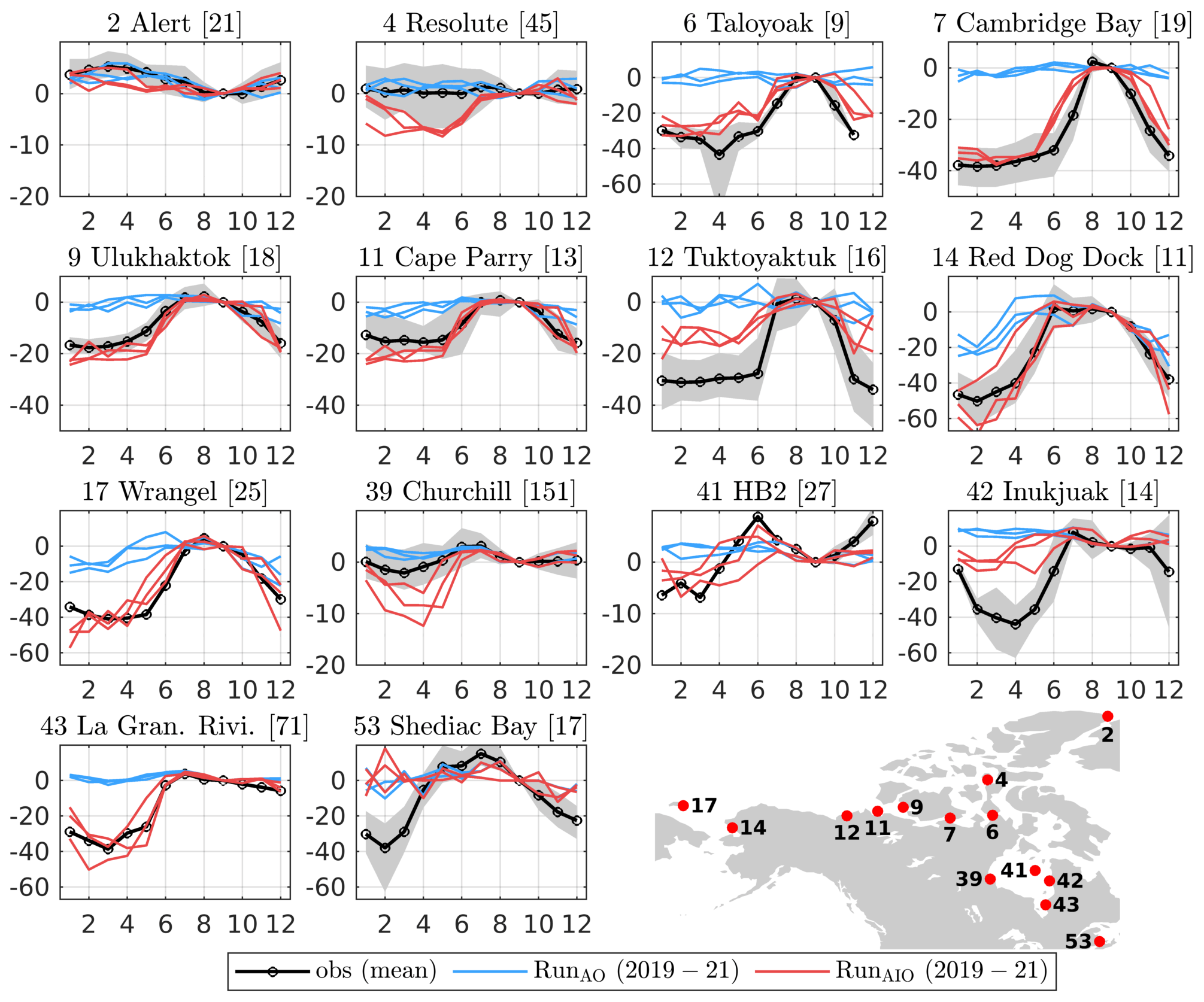
Figure 6 Normalized monthly M₂ amplitude anomaly ($\mathrm{\Delta }{\stackrel{\mathrm{̃}}{A}}_i$; %) relative to September at 14 selected stations. Observed mean (black line) and 10th–90th percentile range (gray shading) are presented, based on available data from 1957–2022. Model predictions from 2019–2022 are provided by Run_AO (blue lines) and Run_AIO (red lines). The title of each subplot gives the station code, station name, and averaged M₂ amplitude (in cm) in September (number in square brackets). The locations of selected stations and their numbering are shown in the bottom right panel.

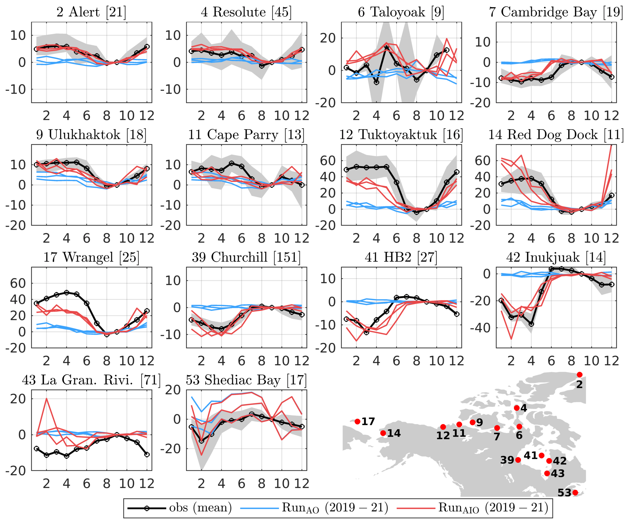
Figure 7 Same as Fig. 6 but for the monthly M₂ phase anomaly (Δϕ_i, ^∘) relative to September.

Figures 6 and 7 show monthly time series of $\mathrm{\Delta }{\stackrel{\mathrm{̃}}{A}}_i$ and Δϕ_i at 14 stations. Selected stations cover various geographical areas, where noticeable amplitude or phase modulations are observed, and they all have a M₂ amplitude of at least 9 cm and a phase modulation of at least 5^∘. Observations show large-amplitude reductions (up to 40 %–50 %; Fig. 6) in the Canadian Arctic (stations 6, 7, and 12), CS (stations 14 and 17), HB (stations 42 and 43), and Northumberland Strait (station 53) and large phase modulations (up to 40–50^∘; Fig. 7) at Tuktoyaktuk (station 12), in the CS (stations 14 and 17) and the eastern HB (station 42). Large modulations can last up to 8 months of the year (e.g., station 12). Model results show that in the absence of ice-induced stress (Run_AO), the predicted $\mathrm{\Delta }{\stackrel{\mathrm{̃}}{A}}_i$ and Δϕ_i are pretty flat, except in the CS (stations 14 and 17), where other processes (e.g., TSI and baroclinicity; see Sect. 6.2.3 for details) contribute up to 20 % to the amplitude modulation. When ice-induced stress is included (Run_AIO), forecasts of $\mathrm{\Delta }{\stackrel{\mathrm{̃}}{A}}_i$ and Δϕ_i are greatly improved at most stations across the season.

We note that there remains room for improvement. For example, $\mathrm{\Delta }{\stackrel{\mathrm{̃}}{A}}_i$ in Run_AIO (Fig. 6) shows slight overestimations (≤ 10 %) at Resolute and Churchill (stations 4 and 39), moderate underestimations (20 %) at Tuktoyaktuk and Inukjuak (stations 12 and 42), and large underestimations (40 %) at Shediac Bay (station 53). We note that Shediac Bay is located near the narrow Northumberland Strait (width of about 13 km) that the $\mathrm{1}/\mathrm{4}$^∘ external model cannot resolve. For Δϕ_i (Fig. 7), the results show moderate (10–20^∘) underestimation at Tuktoyaktuk, Wrangle, and La Grande Rivière (stations 12, 17, and 43) and overestimation at Red Dock dock (station 14). Some of these discrepancies can be explained by the overpredicted amphidrome shifts. We return to this point later (see Sect. 6.2.2).

We next examine the interannual variability in the seasonal M₂ modulation at five permanent gauges during the four ice seasons of the study period (Fig. 8). Observations show interannual variability in both the duration and magnitude of the maximum modulation; changes in duration are up to 2 months (e.g., station 14), while changes in magnitude are up to 10 % in amplitude and 10^∘ in phase. These features are apparently missed by Run_AO, while they are reasonably captured by Run_AIO. One exception is Churchill (station 39), where observations show almost no modulations in amplitude, while Run_AIO generates 5 %–10 % modulations. We note, as before, that observed tides at Churchill may have quality or drift issues (Ray, 2016).

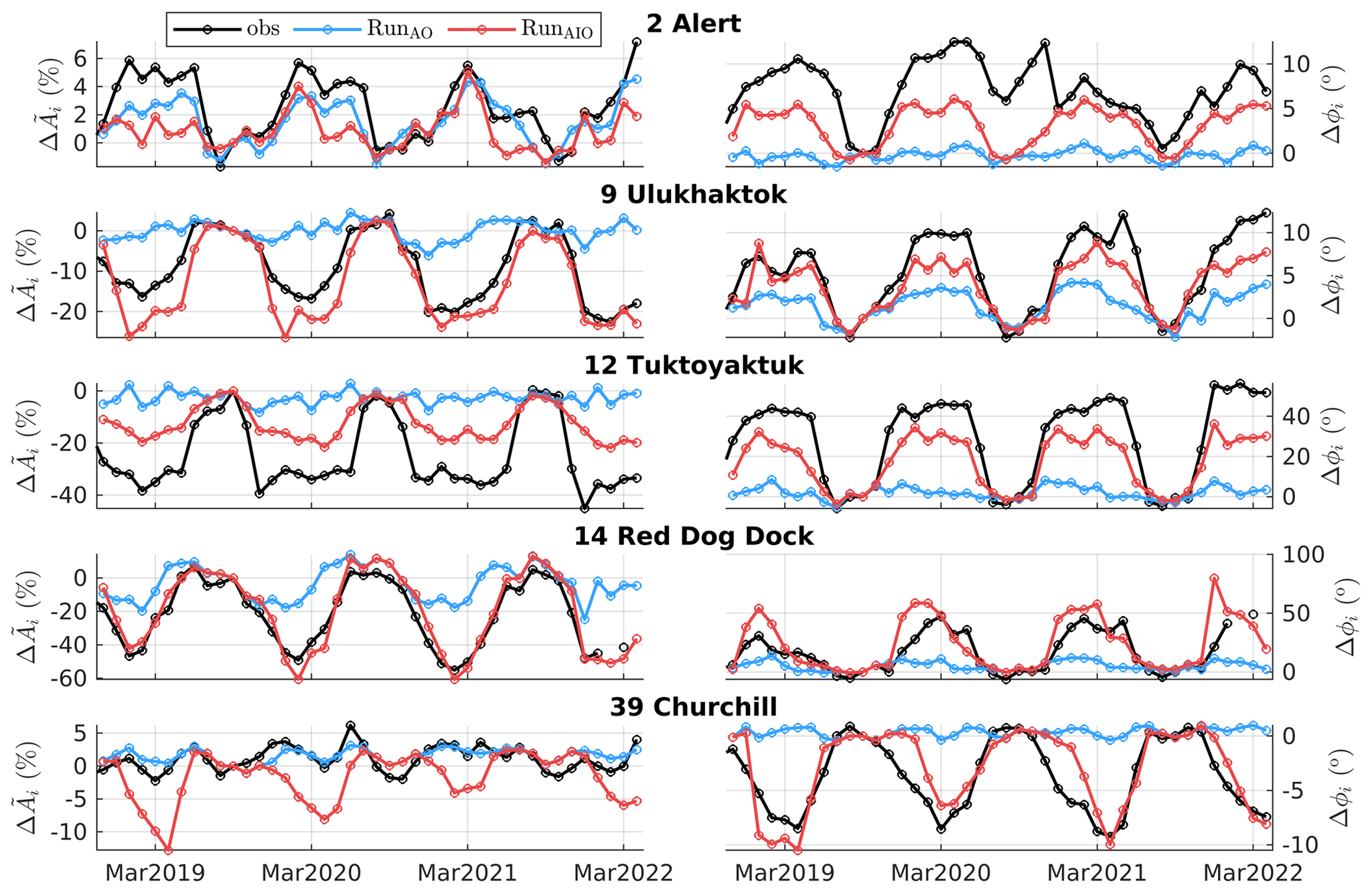
Figure 8 Monthly normalized M₂ amplitude anomaly ($\mathrm{\Delta }{\stackrel{\mathrm{̃}}{A}}_i$; left panels) and phase anomaly (Δϕ_i; right panels) relative to September 2019 at five permanent gauges observed (black), Run_AO (blue), and Run_AIO (red) for the period from November 2018 to April 2022.

6.2.2 Ice-induced amphidrome shift

Ice-induced tidal modulations are associated with shifts of amphidromes. In this section, we examine these shifts. We focus on March, at the peak of the ice cover, and examine the M₂ amphidrome shifts averaged over the study period (Fig. 9). We note that interannual variabilities in shifts are relatively small, except for several small amphidromes in the CS. In general, facing the direction of the shift, amplitudes decrease in the front, while they increase in the back. Still facing the direction of the shift, phase delays and phase advances occur on the left and right sides, respectively. The largest shift is found in the ESS where the amphidrome (marked “A”) moves towards the coast by 90–125 km (note that the arrows in Fig. 9b do not scale with the background distances) due to the ice-induced strong tidal dissipation on the onshore side of the system (see Fig. 5c). The second largest occurs close to the center of the Arctic, where the system (marked “B”) moves towards the Canadian Arctic by 70–90 km. The two shifts are clearly responsible for the dominant large-scale features of M₂ modulations in the Arctic (see Fig. 5). There are also small to moderate shifts (10–50 km) of numerous systems in the Russian Arctic and across the Bering Strait, which affect regional, small-scale modulations.

In the CAA and HB, the frictional effects in Taylor's problem of reflection of Kelvin waves in semi-enclosed basins (Taylor, 1922) explain most of the shifts. The primary effect is the exponential decay of Kelvin wave amplitude in the direction of wave propagation, which causes the amphidromes to shift towards the coast where the reflected Kelvin waves travel (Rienecker and Teubner, 1980; Prinsenberg, 1988; Roos and Schuttelaars, 2011). This behavior applies to both real amphidromes (i.e., amphidrome over the ocean, as marked by “D”–“G”) and virtual amphidromes (i.e., amphidrome over land, as marked by “C” and “H”). We note that real amphidromes may become virtual. This is the case for “D” and “E” in the CAA, which shift over land due to the frictional effects.

These shifts explain the observed and predicted M₂ modulations in the CAA and HB shown in Figs. 6 and 7. For example, the shift of “D” leads to the phase advance at station 7 located to its right side (recall that the relative direction is referred to the direction facing the amphidrome shift). The shift of “C” causes the phase delay at station 4 located to its left side. The shift of “E” is found to be responsible for the overestimated amplitude modulation at station 4, suggesting this shift is overestimated. In the HB, the shifts of “F” and “G” led to the phase advance in most of the HB. In the southern extension of HB, the shift of “H” led to a phase delay on its left side, where station 43 is located, which counters the phase advance induced by the shifts of “F” and “G”. The overall effect is an underestimated phase advance at station 43, indicating that the shift of “H” is overestimated.

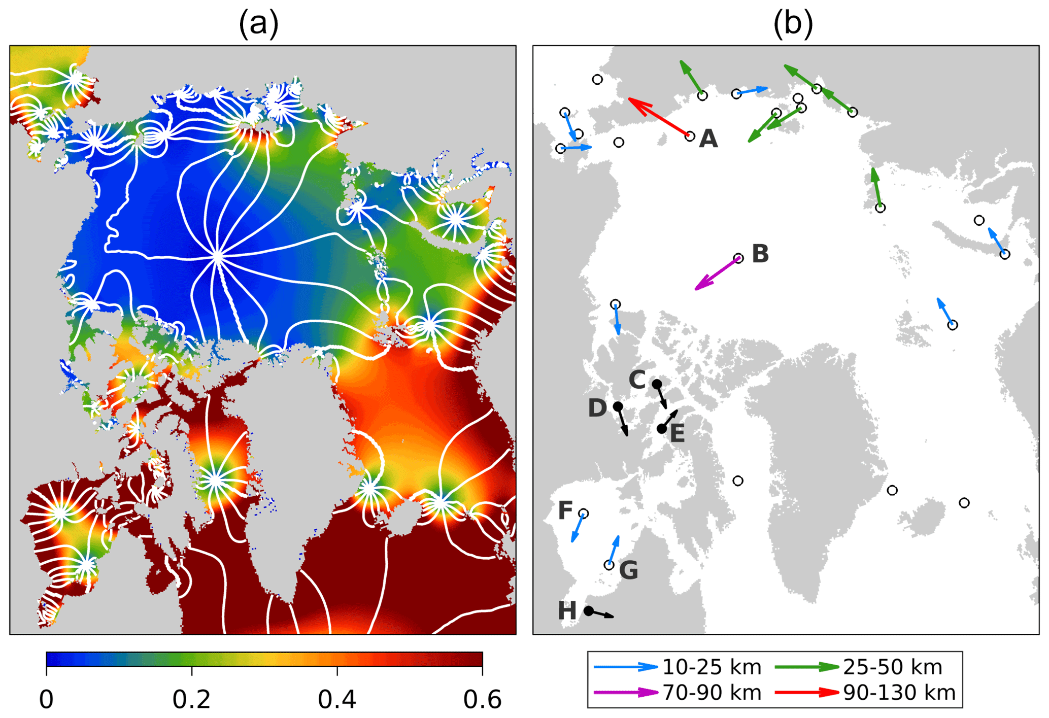
Figure 9 (a) M₂ amphidromes in March predicted by Run_AO, with amplitude (m) in the contour map and phase (every 30^∘) shown with white lines. (b) Ice-induced shifts of M₂ amphidromes in March, taken as the difference in the predicted amphidromic points between Run_AIO and Run_AO. The unfilled circles denote real amphidromes. Their shifts, averaged for 2019–2022, are denoted by colored arrows. The filled circles denote virtual amphidromes or amphidromes that become virtual after the shift. Their positions and shifts (denoted by black arrows) are for illustration purpose only (not to scale).

With ice conditions changing rapidly in the Arctic, it is important to know where the presence of ice or the under-ice friction is most relevant for the amphidrome shifts shown above. Similar to bottom friction, we expect that the impact of the under-ice friction is most relevant over shallow waters where tidal dissipation is significant. We thus conducted four additional sensitivity runs by applying the under-ice friction over regions with water depths of less than 50, 100, 150, and 200 m, respectively. We found that applying the friction over a water depth less than 100 m can reproduce almost all modulations and the associated amphidrome shifts of Run_AIO. These important regions (see Fig. 1 for bathymetry), combined with significant presence of landfast or non-free drift ice (see the middle panels of Fig. 3), cover the bulk of the ESS and CS and the shallow waters (less than 100 m) of the Canadian Arctic and the HB system. This also indicates that although there are large volumes of landfast ice in the deeper waters (greater than 100 m; middle panels of Fig. 3) of the CAA, due primarily to arch formation between islands, their impact on tides is insignificant.

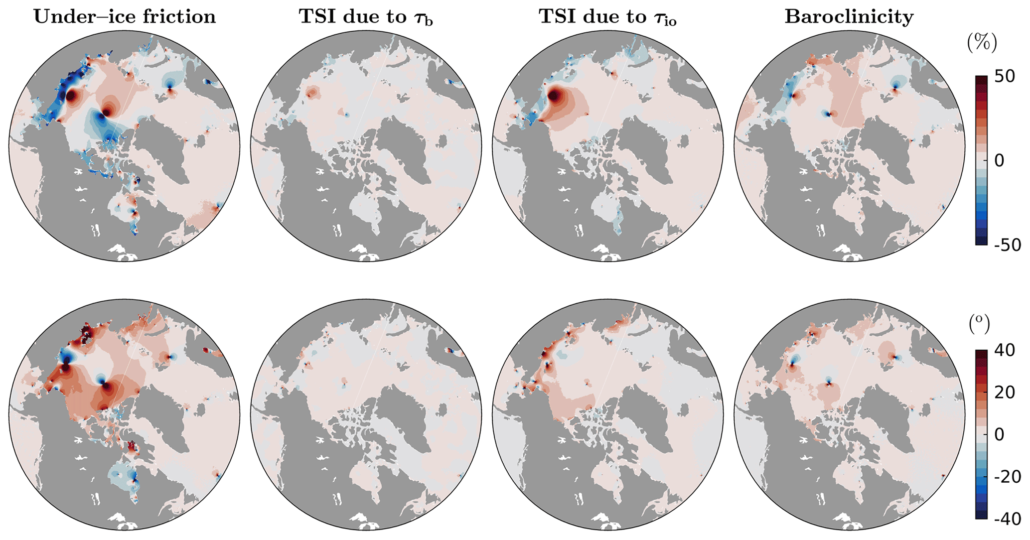
Figure 10 Differences in $\mathrm{\Delta }{\stackrel{\mathrm{̃}}{A}}_{\text{Mar}}$ (top panels) and Δϕ_Mar (bottom panels) for M₂ tides between process-oriented runs, including Run3–Run4 (left), Run2–Run3 (middle left) and Run1–Run2 (middle right), and Run_AIO–Run1 (right), corresponding to effects of the under-ice friction, TSI due to τ_b, TSI due to τ_io, and baroclinicity.

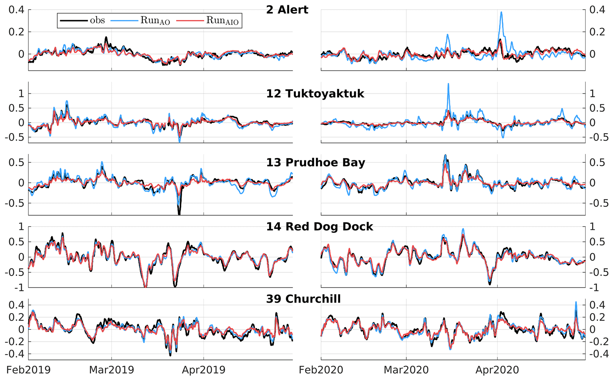
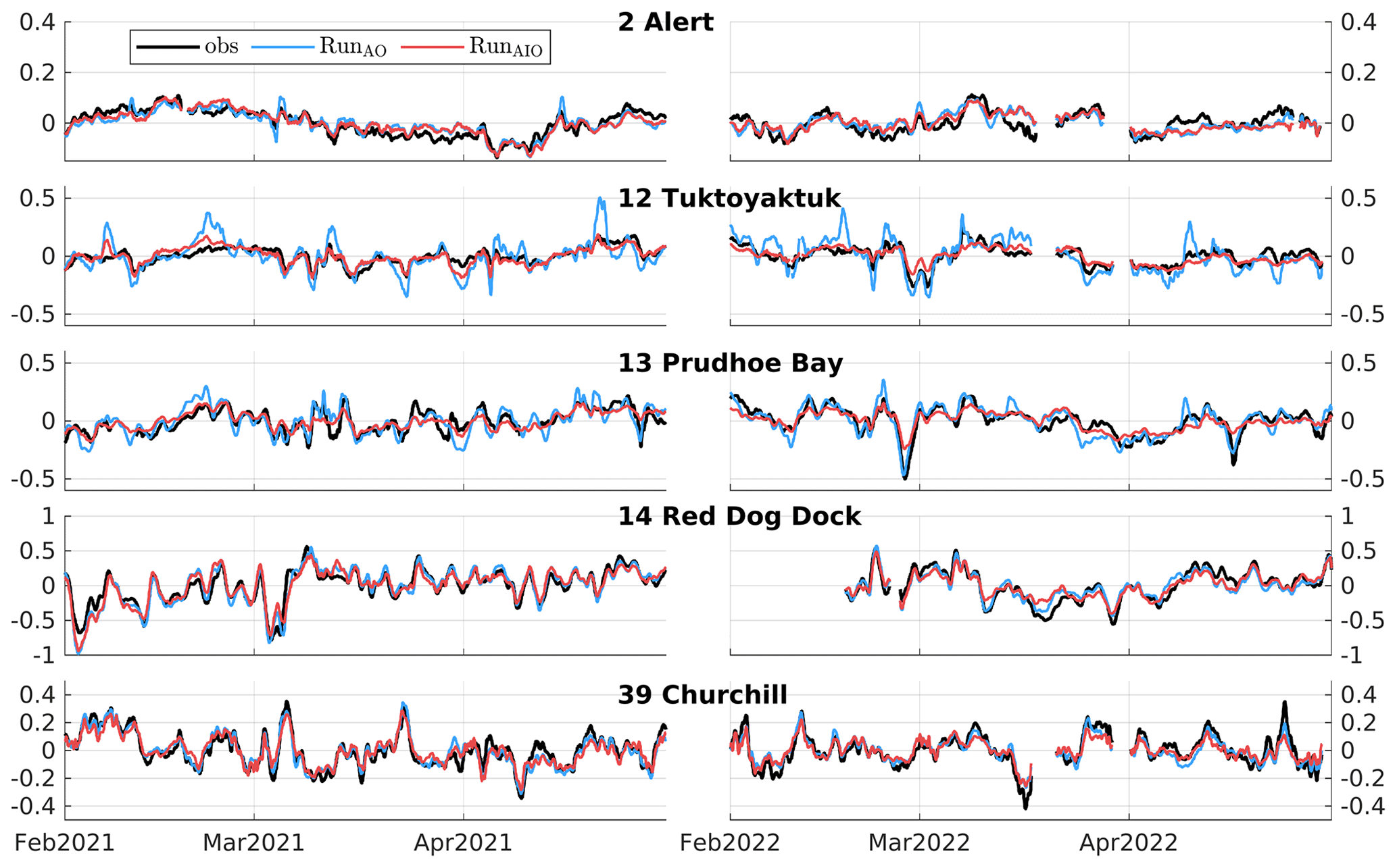
Figure 11 Time series of η_W observed (black) and predicted by Run_AO (blue) and Run_AIO (red) at five permanent gauges during February 2019–April 2020. All values are in meters.

6.2.3 Impact of tide–surge interaction and baroclinicity

We next examine the individual contributions from TSI, baroclinicity, and under-ice friction to $\mathrm{\Delta }{\stackrel{\mathrm{̃}}{A}}_{\text{Mar}}$ and Δϕ_Mar for M₂ (Fig. 10), based on process-oriented runs (Runs 1–4; Table 2). As expected, the under-ice friction (left panels) has the largest influence, while the effect of TSI due to bottom stress is negligible (middle left panels), due to weak bottom currents. The effects of TSI due to τ_io (middle right panels) and the effects of baroclinicity (right panels) are non-negligible. The two mechanisms act in different ways, leading to different spatial and temporal signatures. Strong TSI due to τ_io occurs predominantly over the ESS and CS in March, due to the combination of large ice cover and strong wind-driven surface currents induced by frequent winter storms. Its main effect is to reduce the local M₂ amplitude (> 10 %), resulting in shifts in many small to moderate local amphidromes. It also drives a phase delay of 10–40^∘ over most of the ESS, CS, and Beaufort Sea. Overall, over most of the affected areas, this mechanism reinforces the modulations induced by the under-ice friction (compare panels to the left and middle right).

In contrast, we found that modulations induced by baroclinicity occur mainly in September. This is consistent with Müller et al. (2014), who found that the annual maximum tide occurs in summer in the western Yellow Sea and North Sea. This can be explained by baroclinic effects on the vertical profile of eddy viscosity (Müller et al., 2014); the presence of the pycnocline leads to a stabilized water column and thus reduced tidal dissipation through turbulent processes. Baroclinic effects appear to have a larger scale, mainly affecting several relatively large amphidromes in the Arctic (right panels of Fig. 10). In September, relative to March, this mechanism leads to increased amplitudes (up to 10 %) in the ESS, CS, and north of Norway. The corresponding amphidrome shifts are responsible for most of the phase modulations (about 10^∘). Compared to the left panels of Fig. 10, baroclinicity also reinforces the modulations induced by the under-ice friction.

Figure 12 Same as Fig. 11 but for 2021–2022.

6.3 Storm surges

Storm surges are primarily driven by surface winds and air pressure, and they are usually represented as the tidal residuals, the differences between observed water levels, and predicted tides. However, tidal residuals also contain high-frequency contributions, such as instrument errors and seiches (see Fig. 5 of Wang et al., 2022), which could interfere with the comparison of surges. To attenuate such high-frequency contributions, we applied a low-pass filter with a cutoff period of 10 h to tidal residuals to obtain η_S. We further decompose η_S into a wind and pressure-driven component so that

$$\begin{array}{}\text{(17)}& {\mathit{\eta }}_{\mathrm{S}}\approx {\mathit{\eta }}_{\mathrm{W}}+{\mathit{\eta }}_{\mathrm{P}},\end{array}$$

where η_W is the isostatic wind adjustment part of η_S, and η_P is the inverse barometer effect. A significant contribution to the variability in surges comes from η_P, and this part of the surge signal is almost unaffected by τ_io. This causes difficulties in visualizing and analyzing the ice effects. For this reason, in this section we remove η_P from the surge level (${\mathit{\eta }}_{\mathrm{W}}={\mathit{\eta }}_{\mathrm{S}}-{\mathit{\eta }}_{\mathrm{P}}$). To obtain η_P, we produced an inverse barometer-only prediction (i.e., a run driven with surface air pressures only). We then removed the predicted η_P from both observed and predicted η_S. Figures 11 and 12 show time series of observed and predicted η_W at five permanent gauges where the ice effects are sufficiently large to affect η_W. Adding ice effects in Run_AIO significantly improves the model skill during storm events. For example, it attenuates the peaks in η_W by up to 1.0 m at Tuktoyaktuk (station 12) and 0.25 m at Alert (station 2). Low-frequency variability is also improved (e.g., at Alert) due to the persistent presence of sea ice. However, some over-attenuated peaks in η_W are also found, particularly at Prudhoe Bay (station 13) with, for instance, the largest negative η_W in 2019 and largest positive η_W in 2020 (third row of Fig. 11). Further investigation shows that increasing the ice–ocean drag coefficient even to unrealistically large values does not help. This leads us to speculate that ice velocities are underestimated by GIOPS, possibly as a result of insufficient ice break-up during strong storms.

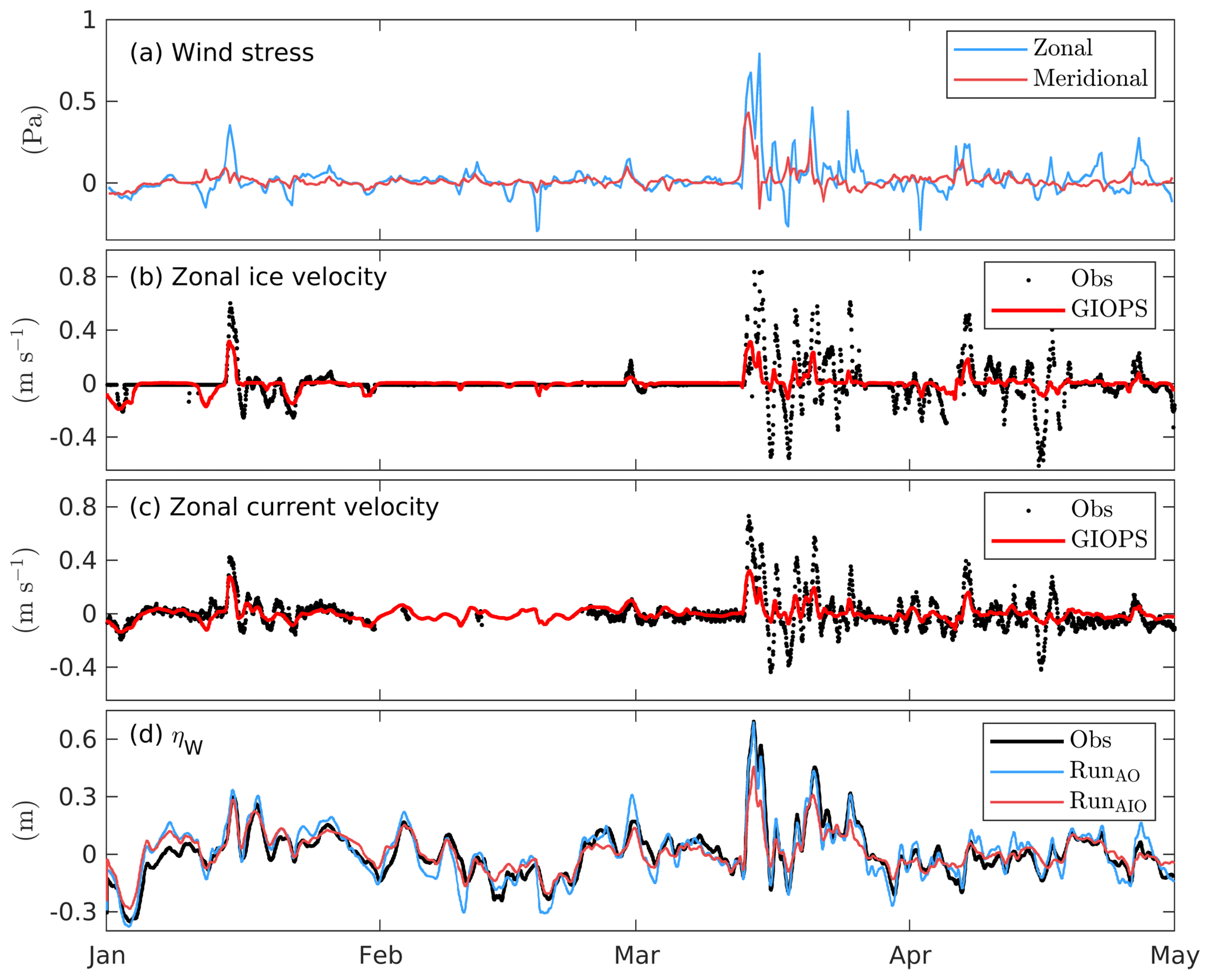
Figure 13 Time series of (a) wind stress provided by the GDPS and (b, c) observed and predicted zonal ice and surface current velocities at an offshore mooring near Jones Islands, located about 50 km west of Prudhoe Bay (station 13), from January to April 2020. (d) Time series of observed and predicted η_W at Prudhoe Bay.

To verify this speculation, we use in situ measurements of ice and surface current velocities collected at an offshore mooring (station S2 offshore in Hošeková et al., 2021) located only about 50 km west of Prudhoe Bay. The wind stress, ice, and current velocities are primarily zonal and parallel to the coast of Prudhoe Bay (Fig. 13). Prior to 15 March, the observed ice was mainly landfast (i.e., ice velocity close to zero), except during a storm event in mid-January. The currents predicted by GIOPS agree well with observations and are consistent with reasonable attenuations of η_W in Run_AIO (Fig. 13d). Around 15 March, during the passage of another storm, observations indicate an ice break-up event associated with strong ice and current velocities (up to 0.8 m s⁻¹). These observed values are greatly underestimated (about 60 %) by GIOPS. After 15 March, the observed ice appears to keep drifting most of the time. This feature was poorly modeled by GIOPS, leading to systematically underestimated ice and current velocities and results in an over-attenuation of η_W in Run_AIO from mid-March to mid-April (Fig. 13d).

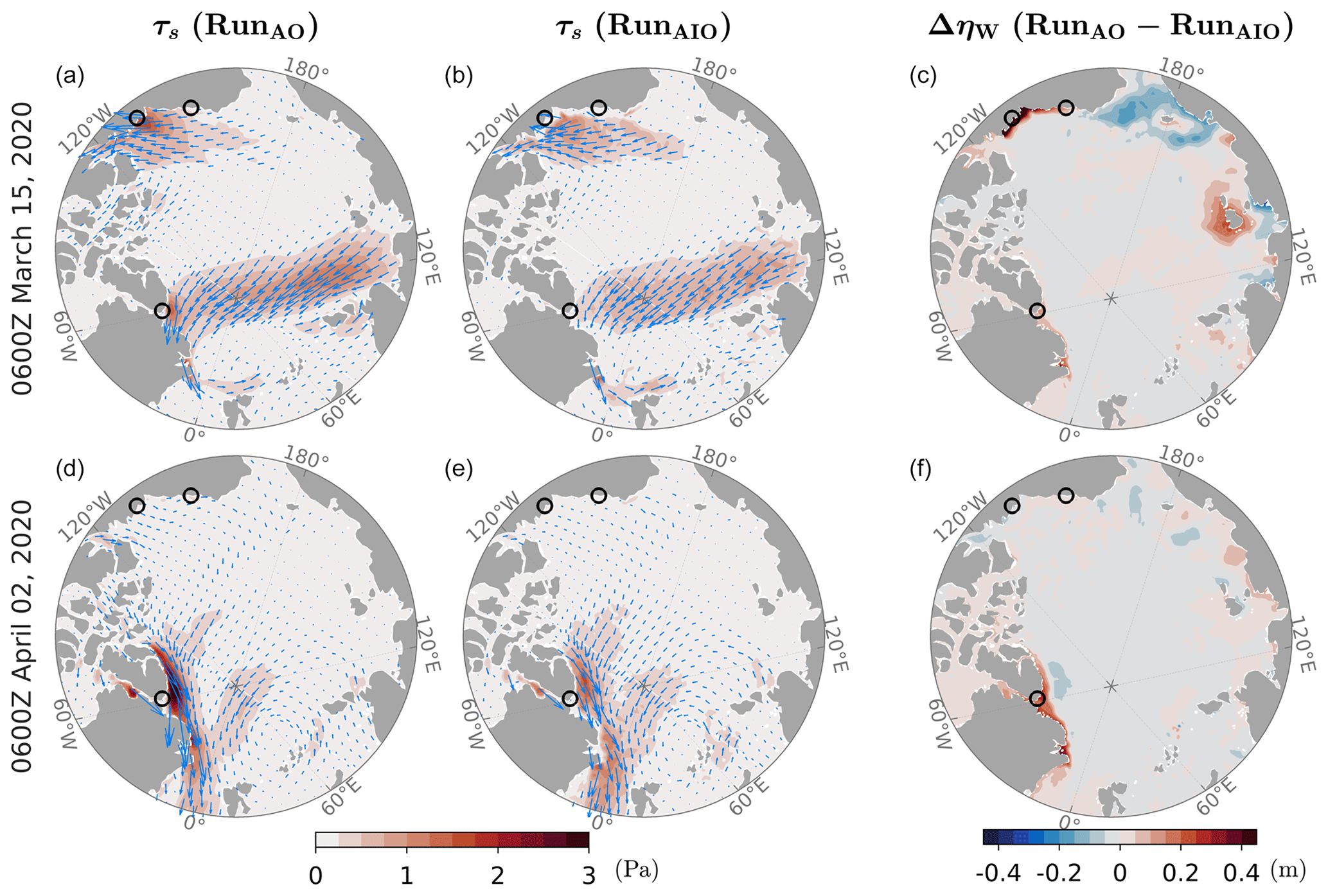
Figure 14 Snapshots of surface stress (τ_s) used in Run_AO (left) and Run_AIO (middle) and differences, Δη_W (Run_AO-Run_AIO), during two storm events on 15 March 2020 (a–c) and 2 April 2020 (d–f). Arrows in the left two columns show the wind stress vectors. Circles show the location of three tide gauges (clockwise from the bottom are station 2 at Alert, station 12 at Tuktoyaktuk, and station 13 at Prudhoe Bay).

In contrast, the successful attenuation of η_W predicted by Run_AIO at Tuktoyaktuk and Alert throughout February–April suggests that sea ice over the two regions has much stronger resistance to large storms. To further illustrate the impact of ice, we examine the ice-induced changes in τ_s during two large storm events on 15 March 2020 at Tuktoyaktuk and 2 April 2020 at Alert (Fig. 14). In both cases, winds blow parallel to the coast (Fig. 14a and d), generating the Ekman setup associated with large η_W predicted by Run_AO, up to 1.3 m at Tuktoyaktuk, and 0.4 m at Alert. In Run_AIO, sea ice associated with strong internal stress greatly reduces τ_s. Reductions in τ_s in the Tuktoyaktuk region are concentrated closer to the coast, and in particular, τ_s is completely shut down at the coast by landfast ice. Reductions in τ_s in the Alert region reach 70 %–80 % for the entire storm. This leads to significant η_W attenuation, spanning about 1000 km along the coast for each storm (Fig. 14c and f), including the western Canadian Arctic (up to 1.0 m attenuation), northeastern Canadian Arctic, and northern Greenland (up to 0.5 m attenuation).

Finally, we note that the comparison of results from Run_AO and Run_AIO also shows large attenuations of η_W up to 1.0 m in the Russian Arctic. Although observations are not available, the estimation is expected to be reasonable considering the large volume of landfast ice in the ESS (see Fig. 3).

7 Summary and conclusions

The present study outlines, and evaluates, a novel approach for adding sea ice effects to a global TWL forecast model. The following two overriding questions are addressed: (1) can we design an efficient parameterization to include ice effects in a global ocean model for forecasting TWL and improve forecast skill in polar regions? (2) Can we isolate and explain the contribution of dominant physical processes (e.g., under-ice friction, baroclinicity, and nonlinear tide–surge interaction) to the seasonal modulation of tides?

The approach incorporates the total (tide plus surge) ice-induced ocean stress by taking advantage of already available external forecast fields (i.e., ice concentration, ice velocity, and surface ocean currents) produced by operational ice–ocean systems. The new method's novel feature is a consistent representation of the tidal relative ice–ocean velocity based on a transfer function derived from ice and ocean tidal ellipses given by external ice–ocean models. This effectively helps circumvent inconsistencies in tides among different models. The approach was applied to ECCC's high-resolution ($\mathrm{1}/\mathrm{12}$^∘) global operational TWL forecast system. The external model is a coarser-resolution ($\mathrm{1}/\mathrm{4}$^∘), data-assimilative global ice–ocean prediction system also running operationally at ECCC. Model predictions of TWL were generated for the period from November 2018 to April 2022, covering four ice seasons.

The impact of adding ice effects was quantified using observed hourly sea level at 58 tide gauges and moorings in ice-infested waters of the Northern Hemisphere. Adding ice effects is shown to help reproduce most of the observed seasonal modulations in the dominant M₂ tide (up to 40 % in amplitude and 50^∘ in phase) in the CS, Canadian Arctic, and HB. The observed interannual variability in the modulation (up to 10 % in amplitude and 10^∘ in phase) during the four ice seasons is also captured by the model, with the addition of ice effects. Improvements are also found, mostly in the Arctic, for other smaller constituents (i.e., S₂, K₁, and O₁; see the Supplement).

The dominant mechanism for seasonal modulations is the under-ice friction due to the presence of landfast or non-free drift ice. It is mostly relevant in areas of shallow waters (less than 100 m) with strong tidal dissipation. These areas cover most of the ESS and CS and parts of the Canadian Arctic and HB system. The under-ice friction leads to amplitude reductions and phase delays. In turn, they can drive large shifts of amphidromes (up to 125 km), resulting in opposite responses (i.e., amplitude enhancement and phase advance). Remote effects of overpredicted shifts help explain some of the discrepancies between observations and model predictions. In addition to the under-ice friction, important contributions from baroclinicity and TSI due to ice–ocean stress were found. The impact of TSI due to ice–ocean stress is found predominantly in March, in shallow areas (i.e., ESS and CS), where large ice cover and strong winter storms occur. In contrast, baroclinic effects are prominent in September, owing to the presence of a pycnocline. The baroclinic mechanism also affect amphidromes and, in particular, the relatively large amphidromes located in the Arctic Ocean. Both mechanisms, TSI and baroclinic effects, generally reinforce the seasonal modulations induced by under-ice friction.

Adding ice effects also greatly improves the model skill in predicting storm surges. This is achieved via ice-induced surge attenuation (up to 1.0 m) over regions (e.g., western and northeastern Canadian Arctic) associated with weak ice mobility and thus strong ice strength. The attenuation is due to considerable ice-induced reductions (70 %–100 %) of the surface stress. Large attenuations, up to 1.0 m, are also predicted along the coast of ESS associated with strong ice strength. Forecast challenges remain in regions with intermediate ice strength (i.e., the coast of northern Alaska), where the inclusion of ice effects leads to over-attenuated surges. Insufficient ice break-up during strong storms in the external model was shown to lead to underestimated ice and current velocities (about 60 %) compared to in situ measurements, and they carry across in the form of over-attenuated surges in the TWL system.

Over the next 100 years, climate change is expected to accelerate, causing a general reduction in ice cover in the Arctic (Pörtner et al., 2022). Our results imply that the reduction in ice concentration and strength over areas of shallow waters, in particular, will dramatically increase tidal amplitudes over most coastal areas. As effects of ice and baroclinicity are expected to decrease and increase, respectively, in winter, tidal amphidromic systems will be pushed towards their ice-free states. The reduced ice cover is also expected to enhance the intensification of winter storms (Crawford et al., 2022), contributing to higher storm surges. Future changes in both tides and storm surges thus pose an increasing risk of coastal flooding and erosion, particularly for coastal areas in the Canadian Arctic currently fully or partially protected by the ice cover.

In terms of future work, we plan to extend the present study to the Antarctic once ice cavities in the Ross Sea and Weddell Sea are included in the external ice–ocean model. It will also be interesting to investigate the dynamical mechanisms behind the observed counterintuitive M₂ modulation in the Ross Sea, as reported by Ray et al. (2021).