the Creative Commons Attribution 4.0 License.
the Creative Commons Attribution 4.0 License.
 | 09 Jun 2023
A comparison of 3-D spherical shell thermal convection results at low to moderate Rayleigh number using ASPECT (version 2.2.0) and CitcomS (version 3.3.1)
Grant T. Euen
Shangxin Liu
Rene Gassmöller
Timo Heister
Scott D. King
Due to the increasing availability of high-performance computing over the past few decades, numerical models have become an important tool for research in geodynamics. Several generations of mantle convection software have been developed, but due to their differing methods and increasing complexity it is important to evaluate the accuracy of each new model generation to ensure published geodynamic research is reliable and reproducible. Here we explore the accuracy of the open-source, finite-element codes ASPECT and CitcomS as a function of mesh spacing using low to moderate-Rayleigh-number models in steady-state thermal convection. ASPECT (Advanced Solver for Problems in Earth's ConvecTion) is a new-generation mantle convection code that enables modeling global mantle convection with realistic parameters and complicated physical processes using adaptive mesh refinement (Kronbichler et al., 2012; Heister et al., 2017). We compare the ASPECT results with calculations from the finite-element code CitcomS (Zhong et al., 2000; Tan et al., 2006; Zhong et al., 2008), which has a long history of use in the geodynamics community. We find that the globally averaged quantities, i.e., root-mean-square (rms) velocity, mean temperature, and Nusselt number at the top and bottom of the shell, agree to within 1 % (and often much better) for calculations with sufficient mesh resolution. We also show that there is excellent agreement of the time evolution of both the rms velocity and the Nusselt numbers between the two codes for otherwise identical parameters. Based on our results, we are optimistic that similar agreement would be achieved for calculations performed at the convective vigor expected for Earth, Venus, and Mars.
- Article
(3626 KB) - Full-text XML
- BibTeX
- EndNote


While there have been significant efforts to develop software capable of modeling mantle convection in a 3-D spherical shell (e.g., Baumgardner, 1985; Bunge et al., 1996; Ratcliff et al., 1996; Zhong et al., 2000; Kageyama and Sato, 2004; Yoshida and Kageyama, 2004; Choblet, 2005; Stemmer et al., 2006; Tan et al., 2006; Choblet et al., 2007; Tackley, 2008; Stadler et al., 2010; Burstedde et al., 2013; Davies et al., 2013; Hüttig et al., 2013), there are few detailed comparison studies of results from more than one code. The modeling software CitcomS has a long history of use in mantle convection studies (e.g., Zhong et al., 2000; Tan et al., 2002; McNamara and Zhong, 2004; Roberts and Zhong, 2004; McNamara and Zhong, 2005; Zhong, 2006; Tan et al., 2006; King, 2008; Foley and Becker, 2009; Sekhar and King, 2014; Liu and Zhong, 2015; King, 2018) and has been compared with analytic kernel solutions and other published results using thermal convection at low Rayleigh number (Zhong et al., 2008). ASPECT (Advanced Solver for Problems in Earth's ConvecTion) is a new-generation, massively parallel mantle convection code combining adaptive mesh refinement (AMR) technology with modern numerical methods (Kronbichler et al., 2012; Heister et al., 2017), built on top of the deal.II finite-element library (Bangerth et al., 2007; Arndt et al., 2021). Three distinct features set ASPECT apart from most other mantle convection codes: (1) its governing equations are dimensional and are written to allow both incompressible and fully compressible flow to be calculated; (2) AMR technology combined with linear and nonlinear solvers allows users to perform mesh adaptation with various refinement or coarsening strategies; and (3) second-order finite elements are employed to discretize the velocity and temperature in the domain, which should lead to better accuracy for a given number of degrees of freedom and a better convergence rate with increasing resolution (Kronbichler et al., 2012; Heister et al., 2017).
There have been a number of studies comparing ASPECT results with other codes using Cartesian geometry (Kronbichler et al., 2012; Tosi et al., 2015; Puckett et al., 2017; Heister et al., 2017; He et al., 2017; Glerum et al., 2018); however, ASPECT has not yet had a systematic benchmark using a 3-D spherical shell geometry. Both the solvers for incompressible Boussinesq Stokes flow and thermal convection of CitcomS have been systematically benchmarked in 3-D spherical shell geometry. The ASPECT solver for incompressible Boussinesq Stokes flow has been benchmarked through analytical propagator matrix solutions (Liu and King, 2019) and a new family of special analytical solutions at spherical harmonic degree 1 and order 0 (Thieulot, 2017). However, the accuracy of the thermal convection calculations (i.e., the energy equation) of ASPECT in 3-D spherical shell geometry has not been tested. No resolution studies of thermal convection in a 3-D spherical shell have been reported for either CitcomS or ASPECT.
In this work we report a comparison of steady-state thermal convection at low to moderate Rayleigh number using both CitcomS and ASPECT. A number of previous studies have focused on the low-Rayleigh-number calculations (7×10³) with viscosity variations up to a factor of 105 (Zhong et al., 2008, and references therein). Zhong et al. (2008) also includes calculations of Rayleigh number 105, a more moderate value, with viscosity variations up to a factor of 30. These allow for steady-state solutions that facilitate comparison between codes. In this work we include both Rayleigh number 7×10³ and 105 calculations. We report the Rayleigh number using the traditional definition where the length scale (D) is the thickness of the spherical shell rather than the radius of the planet. In addition, we reproduce these calculations on a number of different resolution meshes to document the convergence of the globally averaged diagnostics of the steady-state temperature and velocity fields, including root-mean-square (rms) velocity, mean temperature, and Nusselt number at the inner and outer boundaries of the shell.
The conservation of mass, momentum, and energy equations for an incompressible Boussinesq fluid in their nondimensional forms are given by
where t is time, v is velocity, P is pressure, is the radial unit vector pointing toward the center of the planet, and T is temperature (Schubert et al., 2001).
Table 1Parameters used in Zhong et al. (2008) experiments for ASPECT.
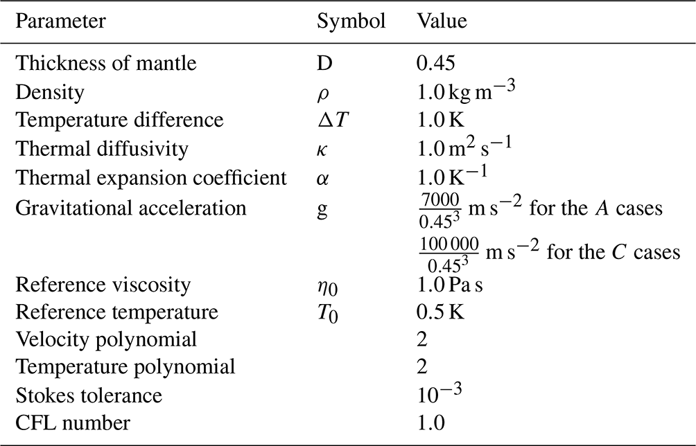
The Rayleigh number and appropriate boundary conditions can describe this problem if all material properties and gravity are held constant. The Rayleigh number is given by
where ρ is the density, α is the coefficient of thermal expansion, g is gravity, ΔT is the change in temperature across the domain, D is the depth of the domain, κ is the thermal diffusivity, and η is the dynamic viscosity. For this work, the Rayleigh number is defined with viscosity at T=0.5. Because ASPECT by default solves the equations in dimensional form, but this benchmark is calculated using a nondimensional scaling, we report the parameters used in the ASPECT calculations to achieve a Rayleigh number of 7×10³ and 105 in Table 1. Boundary conditions are set to be free slip for the inner and outer shell velocity. Temperature is set to a constant T=0 on the outer boundary and T=1 on the inner boundary. The thickness of the shell is set to 0.45, with an inner boundary radius, rb, of 0.55 and an outer boundary radius, rt, of 1.0. By using these values, as well as values of 1 for most other parameters, the Rayleigh number can be controlled by the value of gravity alone (Table 1).
For the ASPECT calculations, we use version 2.2.0 (Bangerth et al., 2020b; Kronbichler et al., 2012; Heister et al., 2017; Bangerth et al., 2020a) published under the GPL2 license to solve Eqs. (1)–(3) using the Boussinesq formulation option. For CitcomS we use version 3.3.1 (Tan et al., 2006; Zhong et al., 2000; McNamara and Zhong, 2004; Moresi et al., 2014), which is also published under the GPL2 license. Both codes are available from the GitHub repository of the Computational Infrastructure for Geodynamics (CIG).
The cases that we consider use temperature-dependent, nondimensional viscosity expressed as
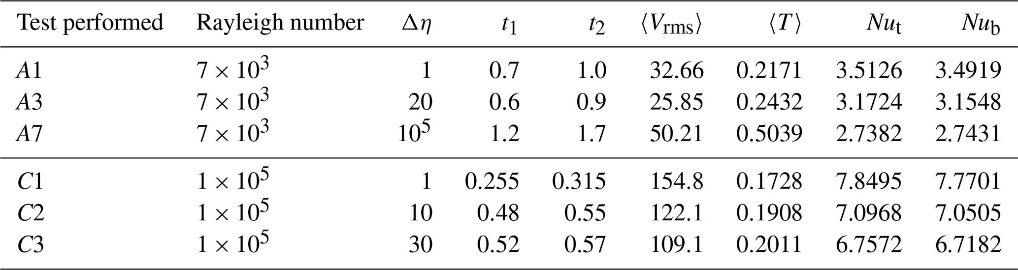
where E is a viscosity parameter similar to activation energy and T is temperature. Following the model naming convention used in Zhong et al. (2008), the letter A refers to cases with Rayleigh number 7×10³ in a tetragonal steady state, while the letter C refers to cases with Rayleigh number 105 in a cubic steady state. The numbers following the letter represent each individual case, which differ by their total variation in viscosity, Δη=eE. We focus on a limited number of viscosity variations, ranging from Δη=1, or constant viscosity, to Δη=105. The value of Δη for each case tested in this study is reported in Table 2.
Table 2Values of the A and C cases presented in this work taken from Zhong et al. (2008). The A cases used a 32-element radial mesh with refinement at the top and bottom. The C cases used a 48-element radial mesh with refinement at the top and bottom.
We compare the results from ASPECT and CitcomS on a variety of meshes and we report the top and bottom Nusselt number, mean temperature, and rms velocity. The Nusselt number, Nu, is the ratio of convective to conductive heat transfer normal to the boundary of the domain. We report the top and bottom Nusselt numbers, defined as
and
where Qt and Qb are the surface and bottom heat fluxes, respectively; rb=0.55; and rt=1.0. We also report the mean temperature and the spherically averaged rms velocity. The volume of the spherical domain is given by
This makes the mean temperature
and the spherically averaged rms velocity
The values of the rms velocity, mean temperature, and top and bottom Nusselt numbers are averaged over the same nondimensional time intervals as those reported in Zhong et al. (2008) (Table 2).
ASPECT uses quadratic velocity and temperature elements by default and has the capability to refine the mesh based on a variety of measured properties of the solution. CitcomS, by comparison, uses linear velocity and temperature elements with a mesh spacing that remains fixed throughout the calculation. The authors of Zhong et al. (2008) refined the CitcomS mesh at the outer and inner boundaries of the shell. In contrast, in order to facilitate the comparison between ASPECT and CitcomS, we use a uniformly spaced mesh in the radial direction. We test meshes at various refinements, including higher levels than those used by Zhong et al. (2008). In order to have a more systematic view of how increasing resolution improves model accuracy, we chose not to refine the CitcomS mesh in our calculations, and AMR and other mesh refining or coarsening strategies for ASPECT are turned off unless otherwise stated. This allowed us to isolate differences between the two codes stemming from their different numerical methods, as opposed to different mesh structures.
In order to more accurately reproduce the CitcomS results, the rheology (Eq. 5) was added to ASPECT as a standalone plugin, which is possible because ASPECT is written to allow adding new features without modifying the main source code itself. By writing and compiling plugins, a user can modify existing features or add completely new ones. A complete description of how to write plugins is available in the ASPECT manual (Bangerth et al., 2022). Specifically, one plugin was written to implement a Frank-Kamenetskii rheology as a standalone material model, and a second plugin was written to allow multiple spherical harmonic perturbations to be used simultaneously as initial conditions. This was necessary to reproduce the cubic-planform cases later in the study.
For CitcomS we used the default parameter setting in the CitcomS-3.3.1 version from CIG with the following exceptions: down_heavy and up_heavy, which are the number of smoothing cycles for downward and upward smoothing, respectively, are set to 3; vlowstep and vhighstep, which are the number of smoothing passes at the lowest and highest levels, are set to 30 and 3 respectively; and max_mg_cycles is the maximum number of multigrid cycles per solve and is set to 50. Our experience showed that fewer downward and upward smoothing cycles lead to time-dependent results for some meshes, while all the other meshes achieved steady solutions. For example, the mesh for C1 was time dependent, with down_heavy and up_heavy set to 2, whereas when down_heavy and up_heavy are set to 3, the solution was steady, as it was for all other meshes. Increasing these parameters had no discernible impact on the overall run time. We caution the reader that the calculation did not converge using the default setting of these parameters in the 3.3.1 version; therefore, we recommend users set down_heavy and up_heavy to 3.
CitcomS requires the user to specify the coarsest mesh and number of multigrid levels with the formula for each direction being
where nprocx is the number of processors in the x dimension, mgunitx is the size of the coarsest mesh in the multigrid solver, and levels is the number of multigrid levels. For each mesh we use at least three multigrid levels, as experience shows that fewer multigrid levels can lead to convergence problems. The parameters that we use for each mesh is shown in Table 3. Using different parameters leads to small differences in the final global quantities reported in Tables 5–10.
Table 3The mesh structure used for CitcomS calculations. The terms nodex, nodey, and nodez are the number of nodes in each direction for each of the 12 cubes making up the sphere. The formula for each direction is nodex = 1 + nprocx × mgunitx , where nprocx is the number of processors in the x dimension, mgunitx is the size of the coarsest mesh in the multigrid solver, and levels is the number of multigrid levels.
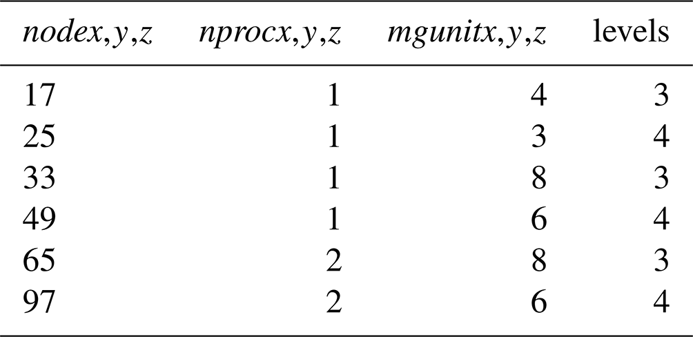
Table 4Degrees of freedom (DoFs) for each resolution of each code. Note that Zhong et al. (2008) did not report the DoFs for their models. The values in parentheses under mesh resolution are the global refinement parameter. In ASPECT, this controls the starting mesh resolution.
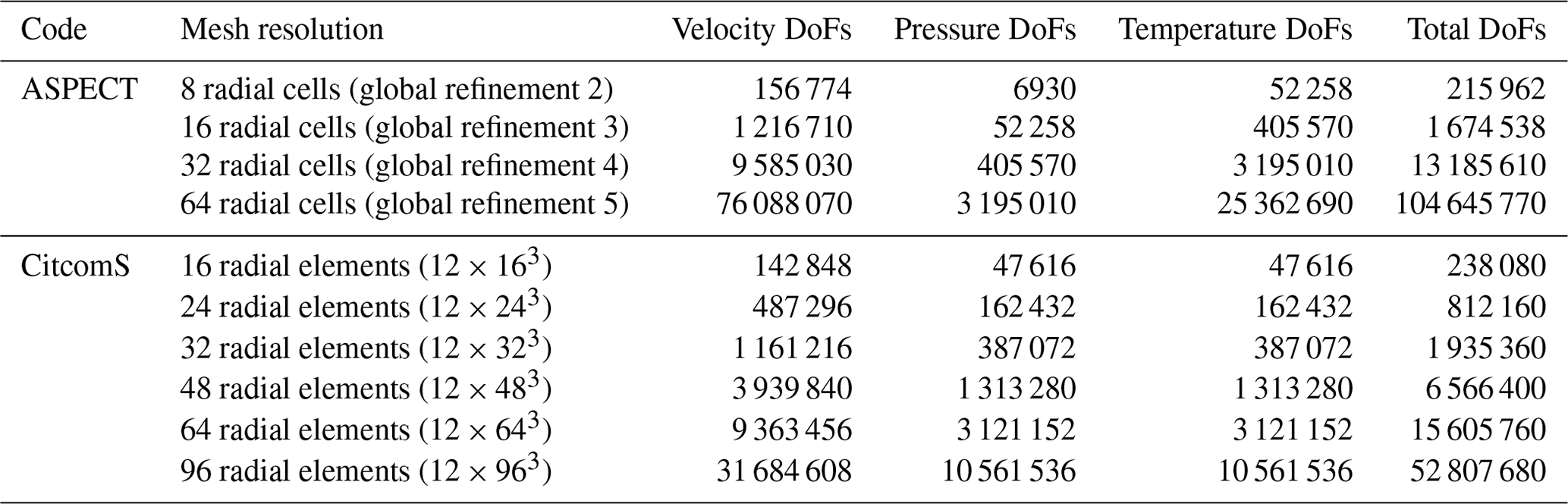
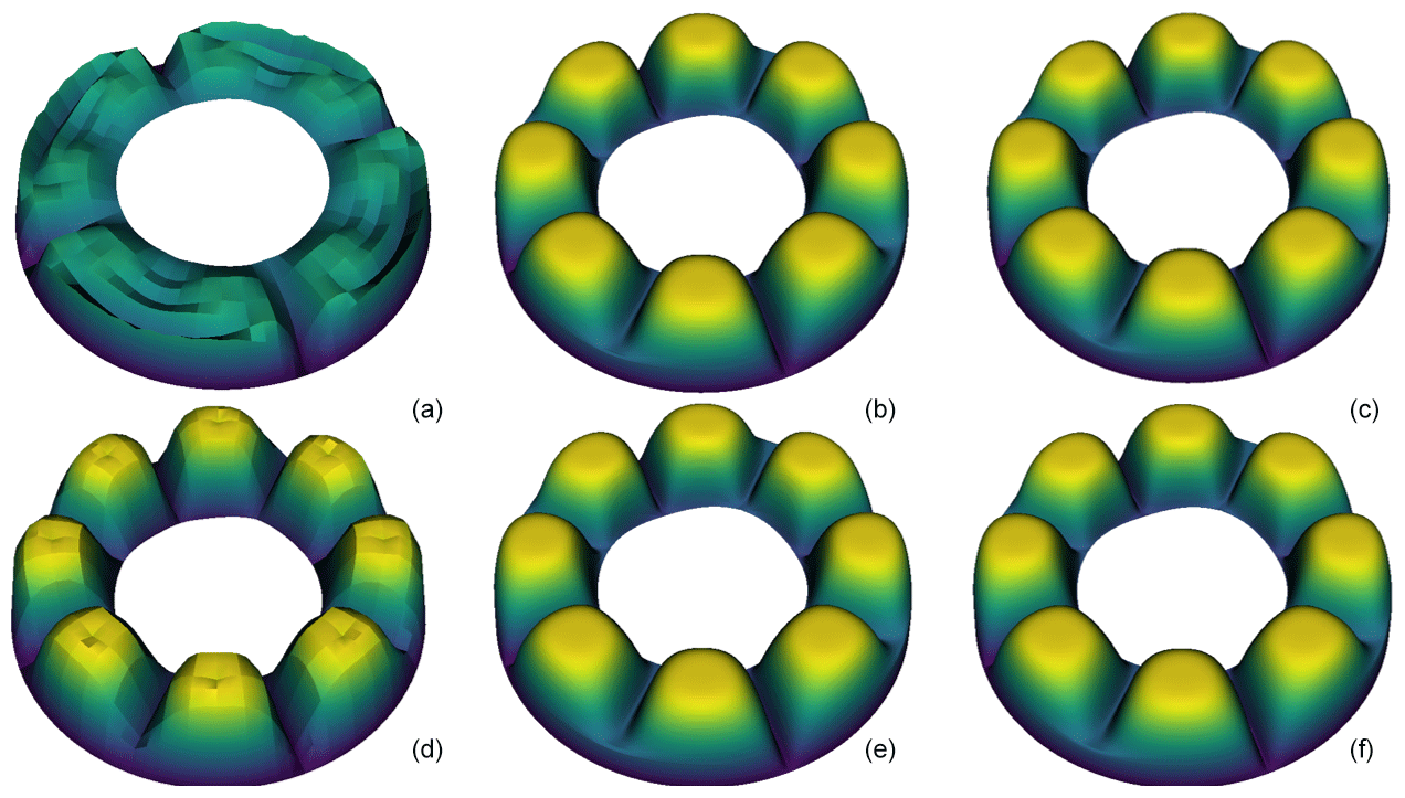
Figure 1Results from the advection-in-annulus benchmark in ASPECT. This shows how mesh refinement influences the heat flux out of the system depending on whether entropy viscosity (a–c) or SUPG (d–f) is used. Both solver schemes produce nearly identical results at moderate mesh refinement (b, e) and high mesh refinement (c, f); however, coarser meshes (a, d) allow for very large differences in heat advection between the two methods. For models in two-dimensions, this is not an issue, as very high refinement can be used without a major increase in computing cost. However, this is an issue for three-dimensional models, as each increase in mesh refinement represents a significant increase in computational resources.
The default ASPECT temperature solver is the entropy viscosity (EV) method (Guermond et al., 2011; Kronbichler et al., 2012). The ASPECT team implemented a streamline upwind Petrov–Galerkin (SUPG) advection-diffusion solver (Brooks and Hughes, 1982) as a part of this work. The SUPG algorithm is also implemented in CitcomS (Zhong et al., 2000) and ConMan (King et al., 1990). ASPECT has several benchmarks included to test robustness of these advection stabilization methods. One test of an advection-diffusion solver is to advect a pattern of known shapes in a 2-D box and rotate them 360∘ at a prescribed velocity (see advection stabilization benchmarks in Bangerth et al., 2022). Another test was created using a simple, four-cell convection pattern in an annulus (Fig. 1). These tests show that the solution using EV is surprisingly diffusive when using more coarse meshes. However, SUPG shows much less diffusion even when coarse meshes are used. With sufficient mesh refinement, the solutions from the two advection stabilization methods are almost identical. This is essentially a non-issue when performing tests in 2-D, as mesh resolution can be adjusted higher without significant change in computational difficulty or run time. However, for 3-D spherical tests, increasing resolution can cause a significant increase in the required computational resources, making highly refined models infeasible. This means that the EV solution is more diffusive for the refinements typically used in 3-D spherical calculations. The ASPECT results shown here primarily use the SUPG implementation, which was part of the ASPECT 2.2.0 release. In the ASPECT 2.2.0 release, the EV parameters have been updated and the results are significantly improved over the results from older versions. In the tables we report the EV results for selected cases.
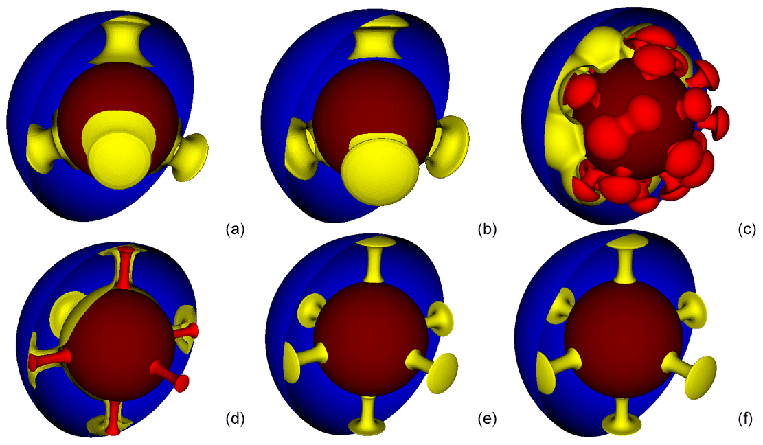
Figure 2Isotherms from Cases A1, A3, A7, C1, C2, and C3 using a 32-cell radially uniform mesh with ASPECT. Isotherms (a), (b), and (c) are the tetragonal-planform cases A1, A3, and A7, respectively. Isotherms (d), (e), and (f) are the cubic-planform cases C1, C2, and C3, respectively. For each image, the central dark red sphere represents the core, the yellow plumes are hotter upwelling material, and the blue half-shell is the surface. In A7 and C1 (c, d) there is also a brighter red layer, which is hotter material than the yellow layer. This is visualized to show more details for the complex convection of A7 and the cores of the plumes of C1. Isotherm values are 1 for dark red, 0.8 for bright red, 0.5 for yellow, and 0.000001 (essentially 0) for blue.
3.1 Low-Rayleigh-number, tetragonal-planform, steady-state thermal convection
In this section we focus on the Rayleigh number 7×10³, tetragonal-planform, steady-state, thermal convection cases labeled A1–A9 in Zhong et al. (2008). The A cases use the same Rayleigh number and initial condition; the label 1–9 refers to the viscosity contrast. Results for the first three cases, A1–A3, were also reported in Ratcliff et al. (1996), Yoshida and Kageyama (2004), and Stemmer et al. (2006).
To create a tetragonal pattern, a degree 3 and order 2 spherical harmonic perturbation is used. The magnitude of this perturbation for both the cosine and sine terms is . The final steady-state pattern of the temperature isotherms can be seen in Fig. 2a and b. The four plumes represent the four corners of a uniform tetrahedron; hence, we refer to this as a tetragonal planform.
To assess how each code handles temperature-dependent rheology, we selected three cases: A1 (constant viscosity), A3 (Δη=20), and A7 (Δη=105). The constant viscosity case provides a baseline result without the added complexity of temperature-dependent rheology. Case A3 (Fig. 2b) was chosen because its viscosity is weakly temperature dependent and can be compared with published results from a number of mantle convection codes. Case A7 was chosen because with this large viscosity contrast the flow transitions into a stagnant-lid mode of convection, causing a much more complex planform (Fig. 2c). Each case was run with both codes using multiple mesh refinement levels Table 4. The results of these runs were then used to extrapolate the theoretical results of a “mesh of infinite refinement” using a Richardson extrapolation. We computed each case using both the default spherical-shell ASPECT mesh and the radially uniform mesh. For CitcomS we used a uniform vertical mesh spacing, which differs slightly from the refined mesh spacing at the top and bottom boundaries used in Zhong et al. (2008). We confirm that we can reproduce the output flow diagnostics reported in Zhong et al. (2008) when using the CitcomS-3.3.1 version downloaded from CIG with the exact parameters used in Zhong et al. (2008). Results for these three cases can be found in Tables 5–7.
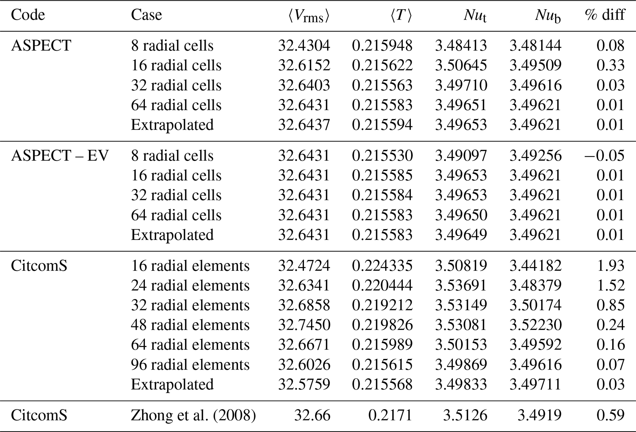
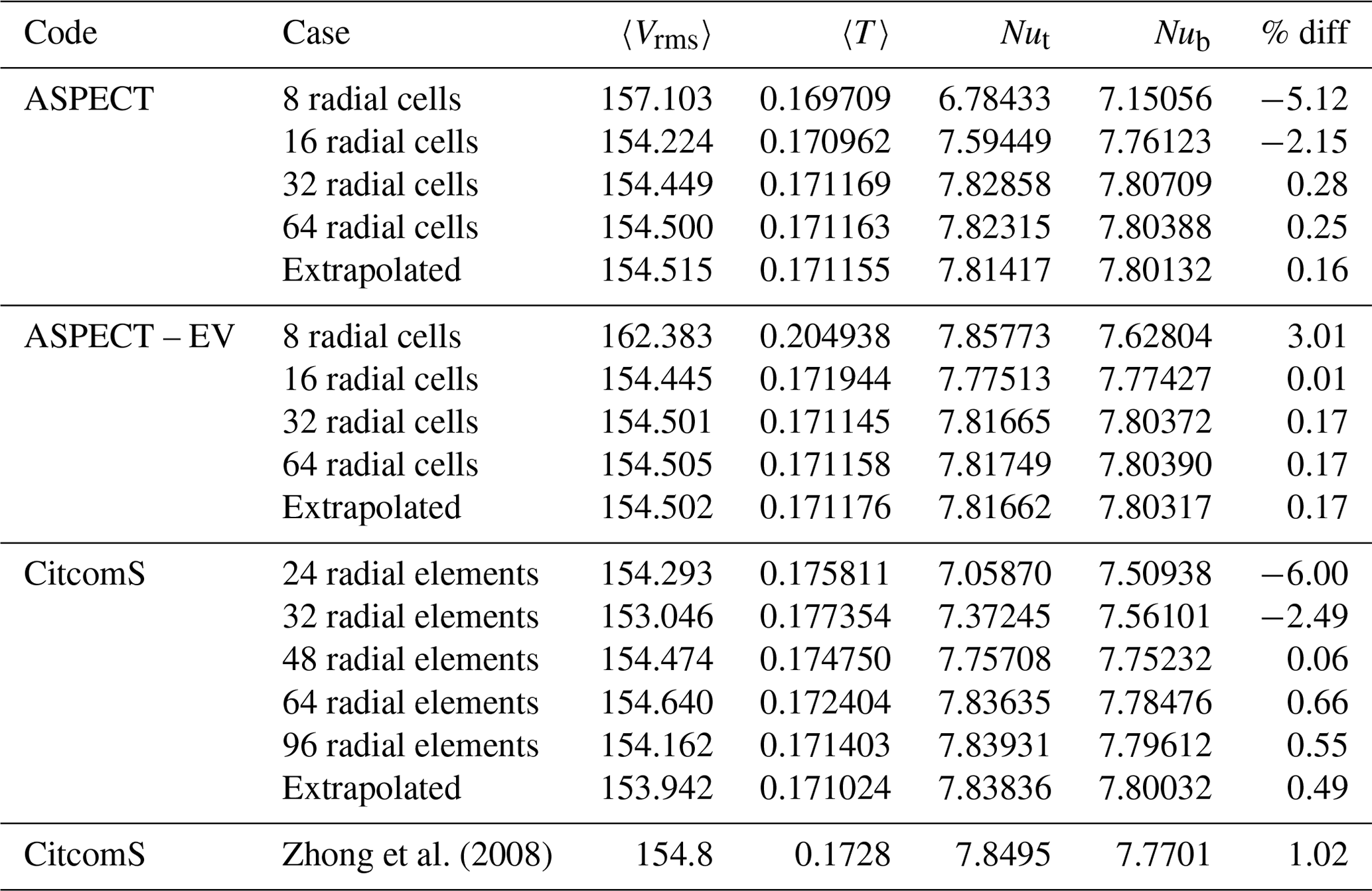
Zhong et al. (2008)Table 5Results for Case A1 on all meshes tested. The column labeled “% diff” represents the percent difference between top and bottom Nusselt numbers for each case. A Richardson extrapolation was applied to the different data sets to estimate the values of a theoretical mesh of infinite refinement.
The results from A1 and A3 on the CitcomS and uniform radial spacing ASPECT meshes are well resolved and in good agreement. Case A7 has larger differences between the two codes, but the overall results are still well resolved and steady. Plots of radially averaged (averaged over shells of constant radii) horizontal and vertical velocity and temperature also show excellent agreement between both codes (Fig. 3).
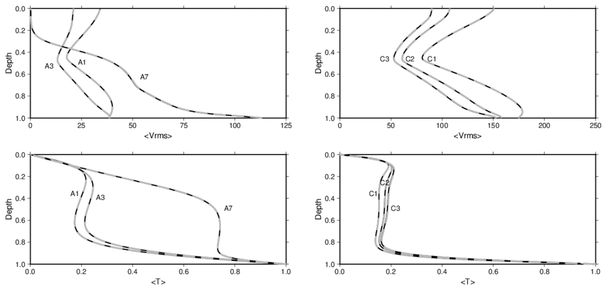
Figure 3Plots of rms velocity and average temperature with respect to depth for all cases tested. Dashed dark grey lines are CitcomS data, and solid black lines are ASPECT data. All cases are in excellent agreement across both codes.
3.1.1 The 3-D results for the constant and weakly temperature-dependent viscosity cases: A1 and A3
We compare the convergence of the solutions from CitcomS and ASPECT for the A1 cases (Fig. 2a) by comparing the rms velocity, mean temperature, and top and bottom Nusselt numbers on a series of increasingly refined meshes. For our ASPECT calculations we use global mesh resolutions of 8, 16, 32, and 64 radial cells to test convergence of model values. For our CitcomS calculations we use 16, 24, 32, 48, 64, and 96 radial elements. Throughout this paper we use cells to describe the ASPECT meshes and elements to describe the CitcomS meshes because this is how the grids are described in the documentation. For CitcomS, where the mesh is divided into 12 cubic regions, each cube has the same number of elements on each side, and thus the 16-radial-element mesh is comprised of elements. For comparison, the results reported in Zhong et al. (2008) were calculated on a mesh with increased refinement at the outer and inner shell boundaries. To facilitate the comparison between our present work and Zhong et al. (2008), we reproduce the results reported in Zhong et al. (2008) in Table 5.
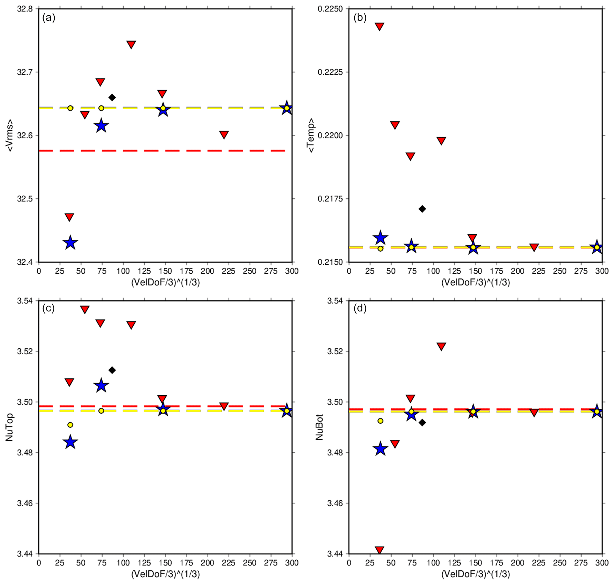
Figure 4The rms velocity, average temperature, and Nusselt number at the top and bottom of the model for Case A1 run at various refinements using CitcomS (red triangles), ASPECT using SUPG (blue stars), and ASPECT using EV (yellow dots). The values reported in Zhong et al. (2008) are also shown (black diamonds). Dashed lines are the extrapolated values for each code. ASPECT and CitcomS show strong agreement in their individual convergence paths with mesh refinement; only rms velocity has a slight difference, though the difference is in the second decimal place.
The plots of rms velocity, mean temperature, and Nusselt numbers at the outer and inner shell boundaries on different meshes for each code (Fig. 4) share a number of common features. For each code, as we increase the mesh size, the values of mean temperature, rms velocity, and top and bottom Nusselt number converge. The top and bottom Nusselt numbers converge to within 0.07 % for CitcomS and 0.01 % for ASPECT, which is to be expected as the top and bottom Nusselt numbers should be equal if the codes conserve energy. The ASPECT mesh produces nearly identical results, with differences only appearing well past the number of significant figures reported by Zhong et al. (2008). Radially averaged values also show nearly identical solutions (Fig. 3). We then extrapolate the values to an infinitesimal mesh using a Richardson extrapolation (Table 5). These extrapolations are slightly different than the values determined by Zhong et al. (2008); however, this is not surprising because Zhong et al. (2008) reported the values from a single 323 mesh with refinement near the surface and the base with no extrapolation to an infinitesimal mesh spacing. The ASPECT results for coarse meshes are closer to the extrapolated value than the CitcomS results for the same mesh, which is not surprising because ASPECT uses second-order elements, whereas CitcomS uses first-order elements. One might argue that the 32 radial cell ASPECT results should be compared with the 64 element CitcomS results. We note that for ASPECT cases A1, the Entropy viscosity results are almost identical to, and in some cases superior to, the SUPG results (Table 5).
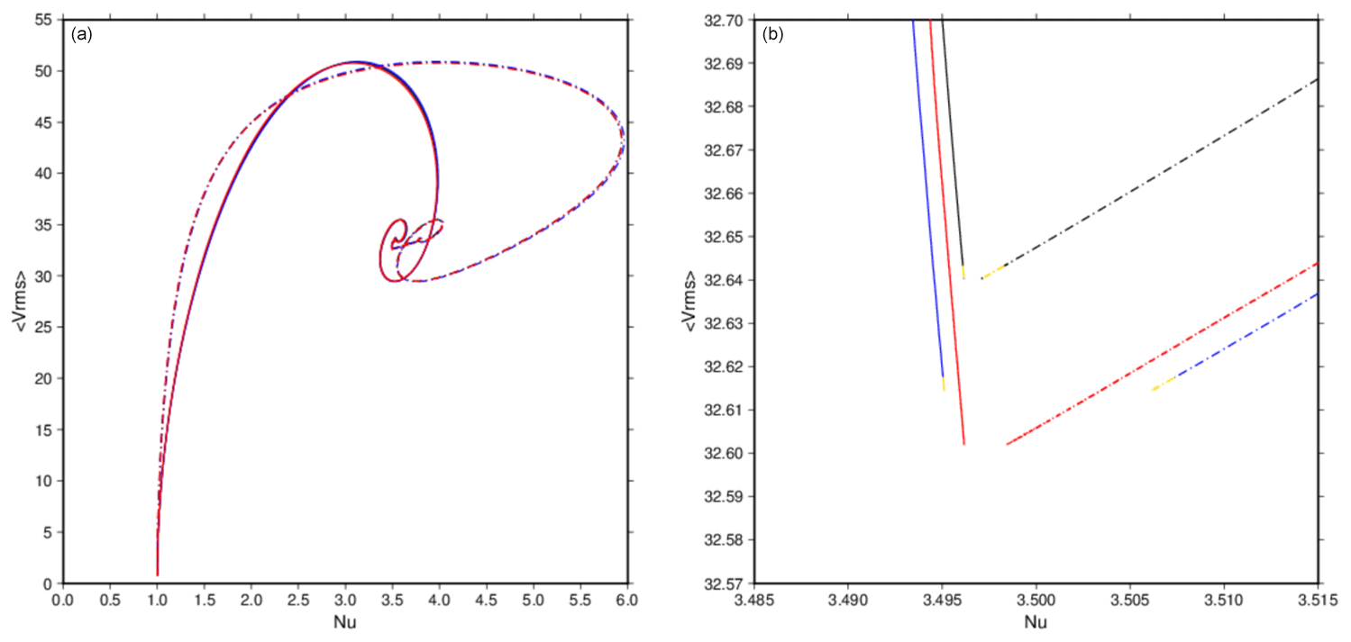
Figure 5The rms velocity plotted against Nusselt numbers at both the top (dashed lines) and bottom (solid lines) of the model for Case A1 run using ASPECT at mesh refinements 12×163 (blue) and 12×323 (black) and CitcomS at mesh refinement 12×963 (red). In the ASPECT runs, gold segments represent the interval used in Zhong et al. (2008) to calculate averages (Table 2). These panels show the similarity in solution between the two codes. It also shows that the model is steady; most of the change happens in the early stage. As the solid and dashed lines approach each other, they slow down. The averaging interval accounts for about one-third of the model runs but are only small pieces of each line.
We also show that in addition to the small differences in the steady-state global quantities between the two codes, the time series evolutions of the global diagnostics follow nearly identical paths. Figure 5 shows rms velocity against both Nusselt numbers for two ASPECT calculations and one CitcomS calculation of Case A1. The path taken to arrive at the solution is the same for all calculations. The specific refinement of the mesh and the code used determines the exact values calculated, but the behavior of the solutions between both codes is consistent.
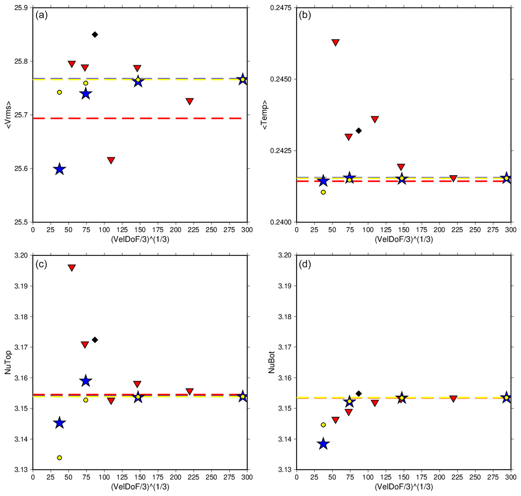
Figure 6The rms velocity, average temperature, and Nusselt number at the top and bottom of the model for Case A3 run at various refinements using CitcomS (red triangles), ASPECT using SUPG (blue stars), and ASPECT using EV (yellow dots). The values reported in Zhong et al. (2008) are also shown (black diamonds). Dashed lines are the extrapolated values for each code. ASPECT and CitcomS show strong agreement in their individual convergence paths. The rms velocity shows a slight difference at the final convergence numbers, though it is small. CitcomS also has an outlier in the convergence path of rms velocity at 12×483 (third point), which can be seen in the average temperature and top Nusselt number as well (though it is not as prominent).
For the A3 cases (Fig. 2b) we compare the results using the same meshes and diagnostics described for A1 (Table 6). Case A3 is very similar to A1 but has a weakly temperature-dependent viscosity, Δη=20 (Table 2). Still, the tetragonal planform is maintained throughout the run. As before, higher mesh refinements allow for greater convergence in both codes. The top and bottom Nusselt numbers converge within 0.08 % for CitcomS and within 0.01 % for ASPECT. The ASPECT results follow a different evolution for convergence with increasing mesh resolution to those for CitcomS, except for the bottom Nusselt number (Fig. 6). The rms velocity and bottom Nusselt number both taper to a high point. The pattern of the average temperature is slightly different, with the coarsest mesh refinement being slightly lower than the other data points. However, the top Nusselt number pattern includes a slightly high outlier at the 16-element (radial) mesh for ASPECT. CitcomS too has an outlier at the 48-element mesh, seen most prominently in rms velocity. We note that for ASPECT Case A3, the entropy viscosity results are almost identical to, and in some cases superior to, the SUPG results (Table 6).
Zhong et al. (2008)Table 6Results for Case A3 on all meshes tested. The column labeled “% diff” represents the percent difference between top and bottom Nusselt numbers for each case. A Richardson extrapolation was applied to the different data sets to estimate the values of a theoretical mesh of infinite refinement.
3.1.2 The 3-D results for the stagnant-lid case: A7
Case A7 has the highest viscosity contrast of all of the cases reported here. Case A6 reported in Zhong et al. (2008) was identified by the authors as a transitional state between mobile-lid and stagnant-lid behavior; all prior models had been mobile-lid examples, and all that followed were stagnant-lid examples. Case A7 was partly chosen because it falls into this category of stagnant-lid behavior. It also has the smallest Δη of the three stagnant-lid cases, the other two being A8 and A9, and thus A7 was also chosen for its relative speed as the time to solve the velocity matrix depends on the viscosity contrast. Case A7 is calculated using ASPECT at mesh resolutions of 8, 16, and 32 radial elements.
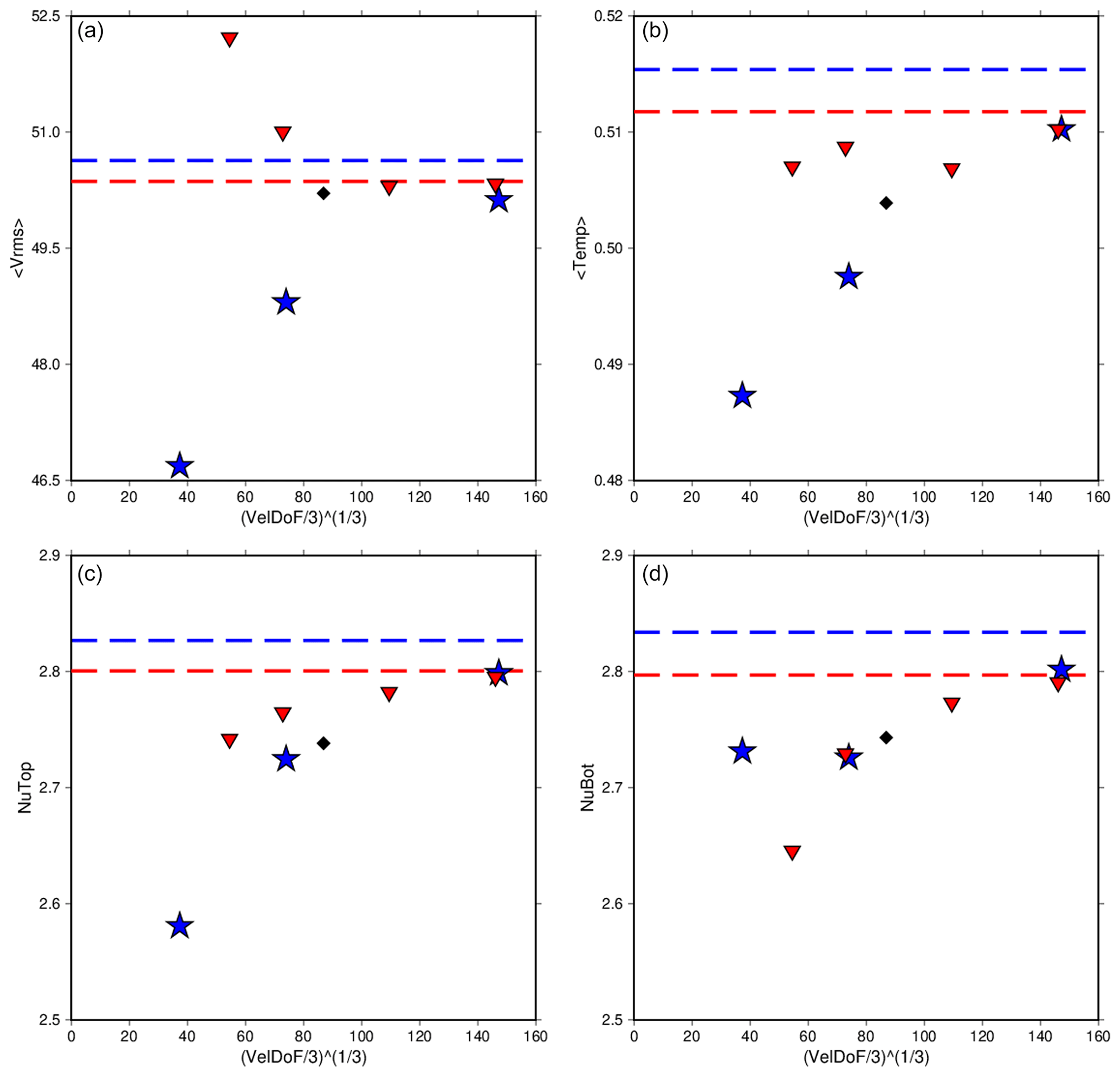
Figure 7The rms velocity, average temperature, and Nusselt number at the top and bottom of the model for Case A7 run at various refinements using CitcomS (red triangles) and ASPECT (blue stars). The values reported in Zhong et al. (2008) are also shown (black diamonds). Dashed lines are the extrapolated values for each code. Of note are the ASPECT solutions for the bottom Nusselt number, which do not show as clear of a trend towards convergence as the other parameters. However, the values are in good agreement with CitcomS, and based on the other parameters they would very likely converge with higher mesh resolution. Extrapolated values between the two codes show small differences for each parameter, larger than previous cases, though higher mesh resolution would again likely cause these values to converge.
Solutions for Case A7 have the most strongly varying results based on the mesh refinement used of all of the A cases (Fig. 7). This is to be expected, as this is the most computationally challenging run in this study. Though it is still amongst the low-Rayleigh-number cases, it has the largest viscosity contrast throughout the mantle.
Zhong et al. (2008)Table 7Results for Case A7 on all meshes tested. The column labeled “% diff” represents the percent difference between top and bottom Nusselt numbers for each case. A Richardson extrapolation was applied to the different data sets to estimate the values of a theoretical mesh of infinite refinement.
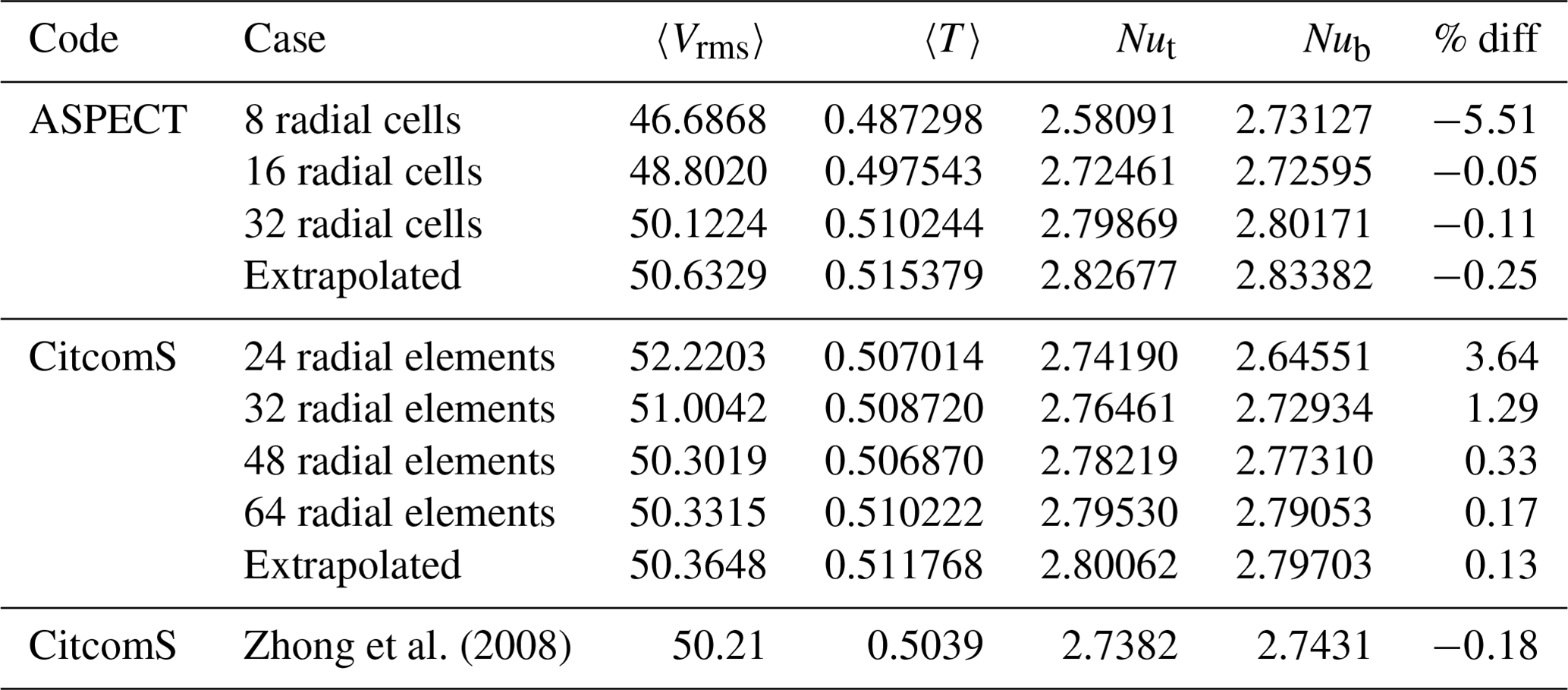
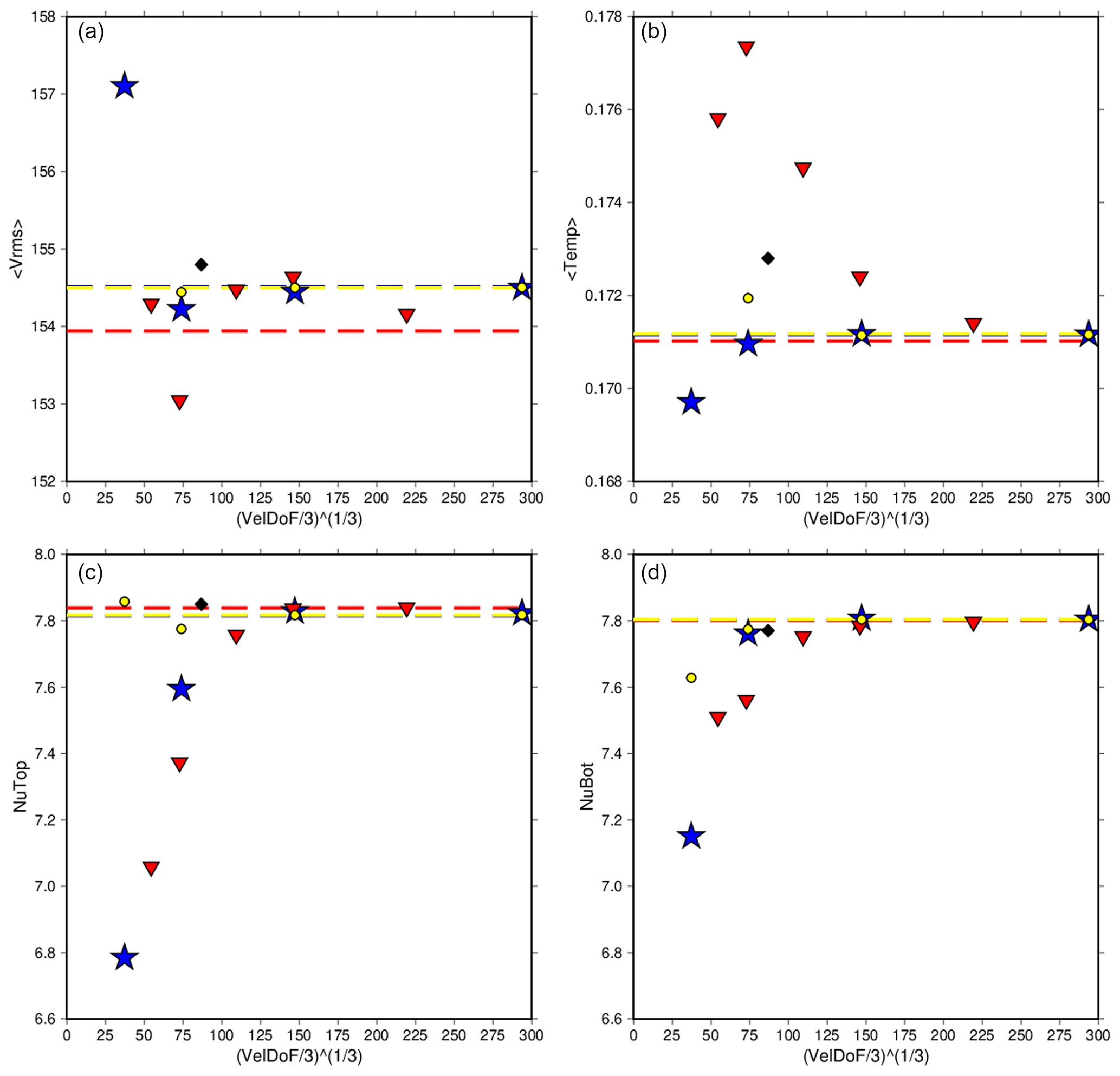
Figure 8The rms velocity, average temperature, and Nusselt number at the top and bottom of the model for Case C1 run at various refinements using CitcomS (red triangles), ASPECT using SUPG (blue stars), and ASPECT using EV (yellow dots). The values reported in Zhong et al. (2008) are also shown (black diamonds). Dashed lines are the extrapolated values for each code. ASPECT and CitcomS show strong agreement in all reported parameters. It should be noted that the coarsest meshes of ASPECT using EV (global refinement 2, yellow dots) are not shown for rms velocity and average temperature. These values are higher than others (Table 8) and only make it more challenging to see the convergence of the rest of the data, and thus they were omitted from this figure.
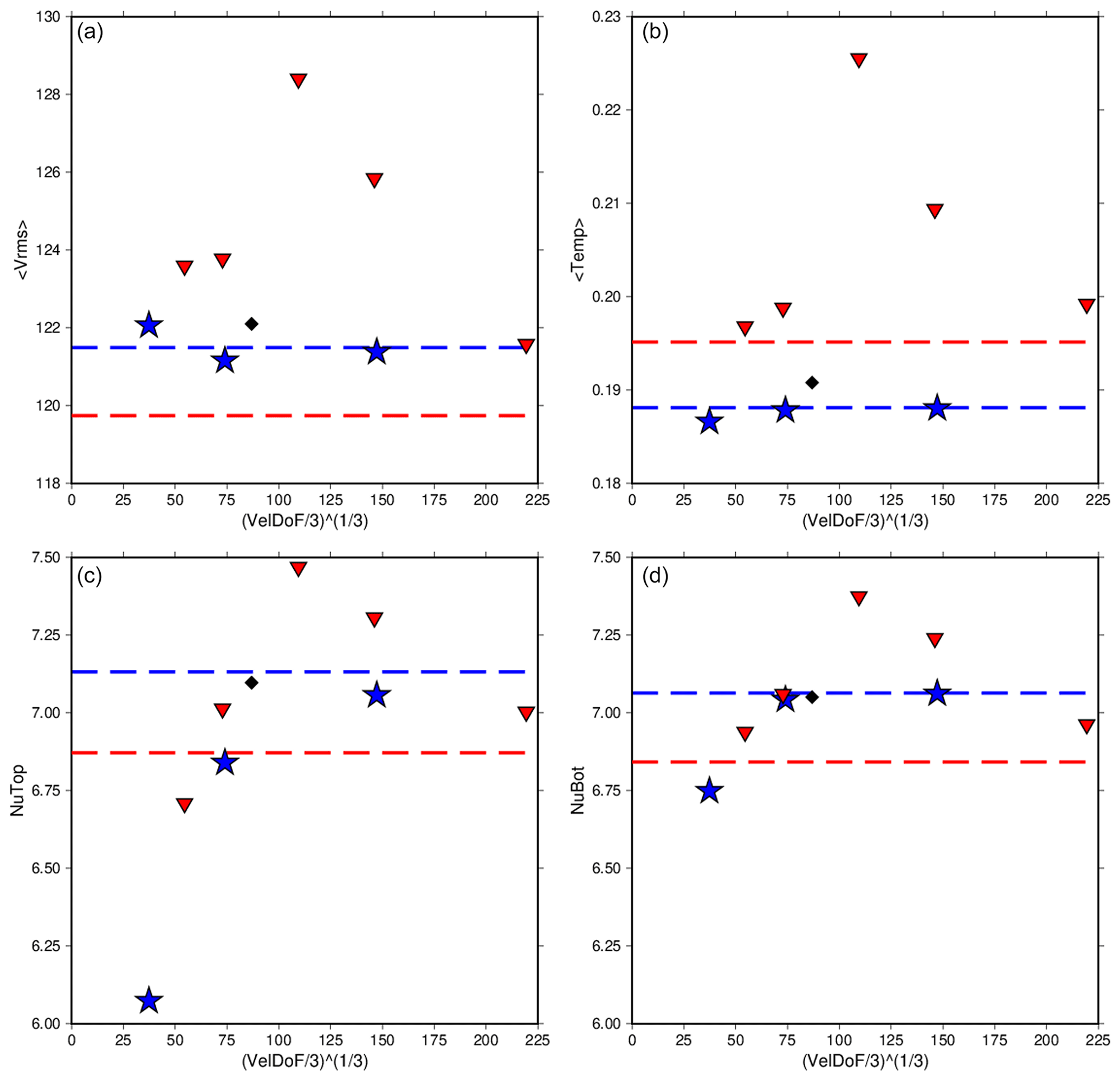
Figure 9The rms velocity, average temperature, and Nusselt number at the top and bottom of the model for Case C2 run at various refinements using CitcomS (red triangles) and ASPECT (blue stars). The values reported in Zhong et al. (2008) are also shown (black diamonds). Dashed lines are the extrapolated values for each code. ASPECT and CitcomS show more of a difference in convergence in this case. CitcomS in particular shows a very different path of convergence between its coarser and finer resolutions. Ultimately both codes come into better agreement at higher resolution, though parameters still show a larger difference than the other reported cases.
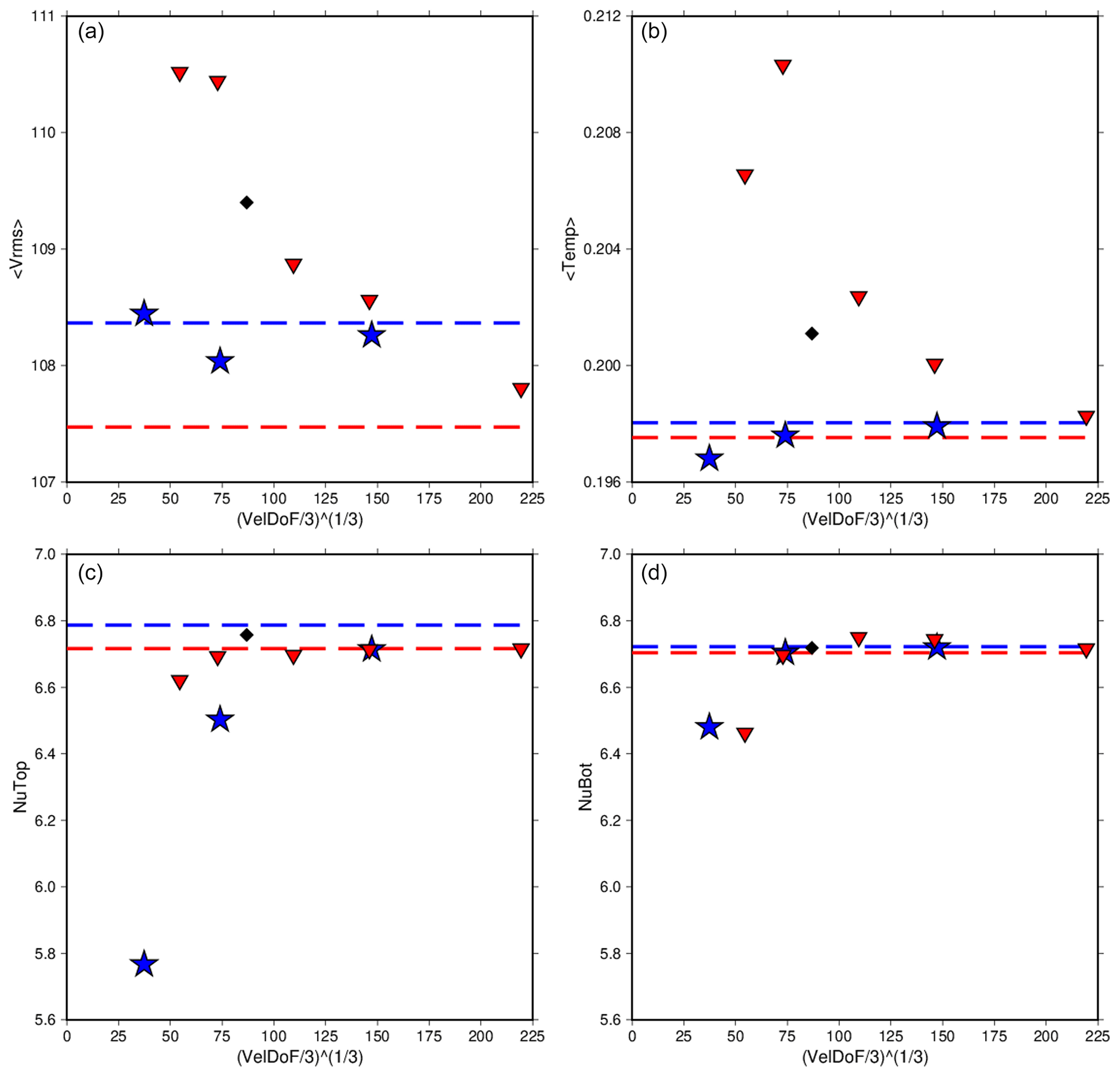
Figure 10The rms velocity, average temperature, and Nusselt number at the top and bottom of the model for Case C3 run at various refinements using CitcomS (red triangles) and ASPECT (blue stars). The values reported in Zhong et al. (2008) are also shown (black diamonds). Dashed lines are the extrapolated values for each code. ASPECT and CitcomS both show strong convergence in all parameters reported. Interestingly, both codes show better agreement than the previous case C2. Extrapolated values for rms velocity and average temperature also show a larger difference from values reported in Zhong et al. (2008) than previous C cases.
Reported values for this case show more difference between the two codes, even at the highest mesh refinements tested (Table 7). Still, the two codes are in good agreement, with radially averaged values from the most refined meshes of both codes being nearly identical (Fig. 3). More data points from further refined meshes would assist in establishing the pattern of convergence; however, at 32 radial elements the computation is already exceedingly costly. Case A7 run to completion using a refinement of 64 radial elements would take weeks of run time on 384 processors; hence, these calculations were not performed. However, the difference between top and bottom Nusselt numbers still show that solutions are well resolved. CitcomS converges to within 0.17 %, while ASPECT converges to within 0.11 %. Isotherms from this case help us to understand the behavior that is not seen in the other cases. The initial tetragonal pattern is lost in this case, as several smaller plumes of hot material upwell throughout the mantle (Fig. 2c). In Cases A1 and A3 the tetragonal pattern is maintained throughout the run (Fig. 2a and b). These results match the behavior reported in Zhong et al. (2008). Looking at the steady global diagnostics reported, it can be seen that both codes are in good agreement, and ASPECT is very likely converging with higher mesh resolution for Case A7.
3.2 Intermediate-Rayleigh-number, cubic-planform, steady-state thermal convection
The C cases have a similar setup to the A cases, with a few notable differences. For their initial condition they use two spherical harmonic perturbations of degree 4 and order 0 and degree 4 and order 4 simultaneously, resulting in the number of plumes increasing from 4 to 6 (Fig. 2d–f). If a cube is envisioned surrounding the model, these six plumes are evenly spaced at the centers of its sides; hence, the planform of the C cases is referred to as cubic. The Rayleigh number is also increased to 105, compared to the tetragonal-planform cases using a value of 7000. While this is still smaller than the Rayleigh number typically used in geodynamic models, it approaches the planetary range. Case C1 is a perfect analogue to Case A1, using a constant viscosity (Δη=1) with the new cubic-planform initial conditions. Cases C2 and C3 use weakly temperature-dependent viscosity, analogous to Case A3 (Δη=10 and 30, respectively). However, they use the final state of C1 as their initial condition rather than starting at time 0. For example, cases of C2 and C3 on an 8-radial-element mesh resolution used the final solution of Case C1 on an 8-radial-element resolution. ASPECT runs of C2 and C3 also kept the mesh type consistent for these initial conditions.
The results from all three C cases tested are well resolved and in good agreement between the two codes. Case C2 proved slightly more challenging for CitcomS, but with higher mesh resolution good convergence was achieved (Fig. 9). Radially averaged values also show strong agreement between both codes for all C cases (Fig. 3).
3.2.1 The 3-D results for the constant viscosity case: C1
As with the tetragonal-planform cases, we compare the convergence of the solutions from CitcomS and ASPECT for the C1 cases (Fig. 2d) by comparing the rms velocity, mean temperature, and top and bottom Nusselt numbers on a series of increasingly refined meshes. For our ASPECT calculations we used the radially uniform ASPECT mesh described previously. We use global mesh resolutions of 8, 16, 32, and 64 radial cells to test convergence of model values. For our CitcomS calculations we use 24, 32, 48, 64, and 96 radial elements. Results reported in Zhong et al. (2008) were calculated on a mesh with increased refinement at the outer and inner boundary of the spherical shell. To facilitate the comparison between our present work and Zhong et al. (2008), we reproduce the results reported in Zhong et al. (2008) in Table 8.
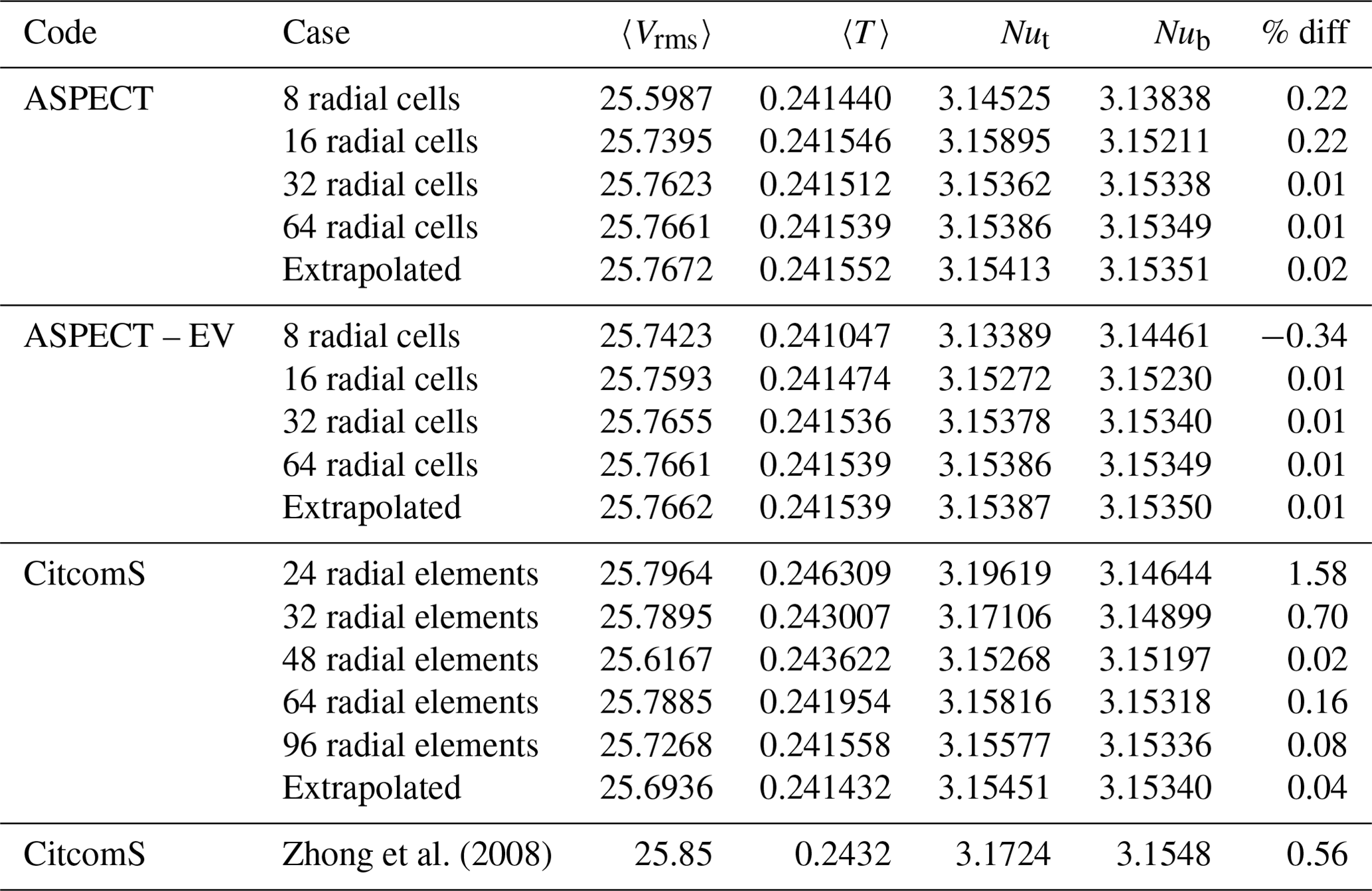
Zhong et al. (2008)Table 8Results for Case C1 on all meshes tested. The column labeled “% diff” represents the percent difference between top and bottom Nusselt numbers for each case. A Richardson extrapolation was applied to the different data sets to estimate the values of a theoretical mesh of infinite refinement.
Plots of rms velocity, mean temperature, and top and bottom Nusselt numbers on different meshes are again produced, with overall convergence increasing with mesh refinement (Fig. 8). The top and bottom Nusselt numbers converge to within 0.55 % for CitcomS and 0.17 % for ASPECT. It should be noted that our CitcomS run using 48-radial-element resolution has an agreement of 0.06 %, an outlier in the convergence trend. Radially averaged plots show strong agreement between the two codes (Fig. 3). We then extrapolate the values to an infinitesimal mesh using a Richardson extrapolation (Table 8). Once again, the ASPECT results for coarse meshes are closer to the extrapolated value than the CitcomS results for the same mesh resolution. Agreement between the two Nusselt numbers for each case actually follows a similar pattern of convergence between the two codes. The resolution of 32-cell radial ASPECT mesh is already within 0.3 % agreement, while CitcomS is only within 2.5 %.
Data points trend smoothly towards convergence for ASPECT, with a slight outlier at 8-radial-element resolution. The rms velocity at that resolution especially falls farther from other data. We note that overall EV produces solutions with Nusselt numbers in better agreement for this case; however, its rms velocity outlier at 8-radial-element resolution is larger. CitcomS data points also trend towards convergence for both Nusselt numbers. The rms velocity and temperature have some outliers at coarse mesh resolutions, though at higher resolutions there is still a clear trend towards convergence. We note that for ASPECT Case C1, the entropy viscosity results are almost identical to, and in some cases superior to, the SUPG results (Table 8).
Zhong et al. (2008)Table 9Results for Case C2 on all meshes tested. The column labeled “% diff” represents the percent difference between top and bottom Nusselt numbers for each case. A Richardson extrapolation was applied to the different data sets to estimate the values of a theoretical mesh of infinite refinement.
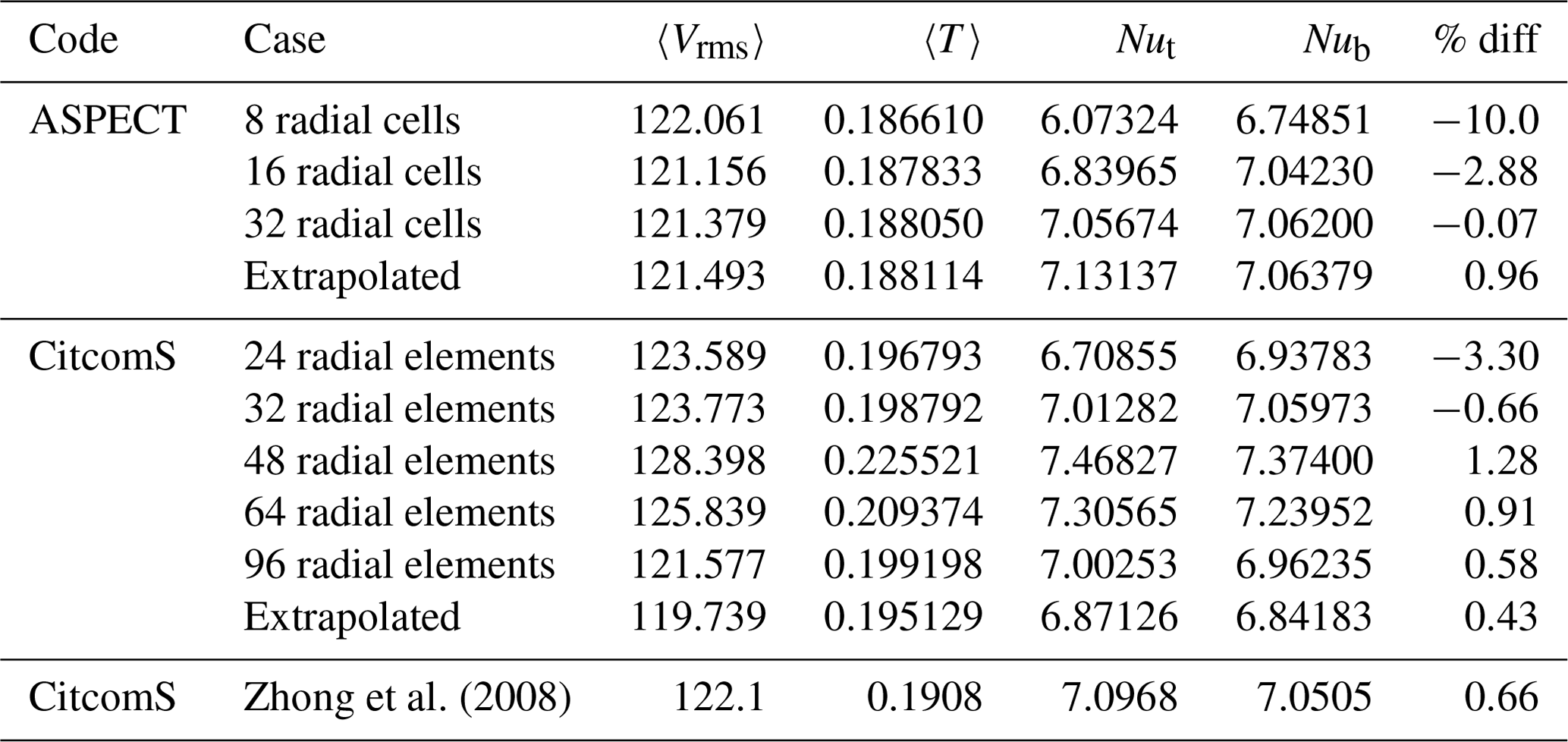
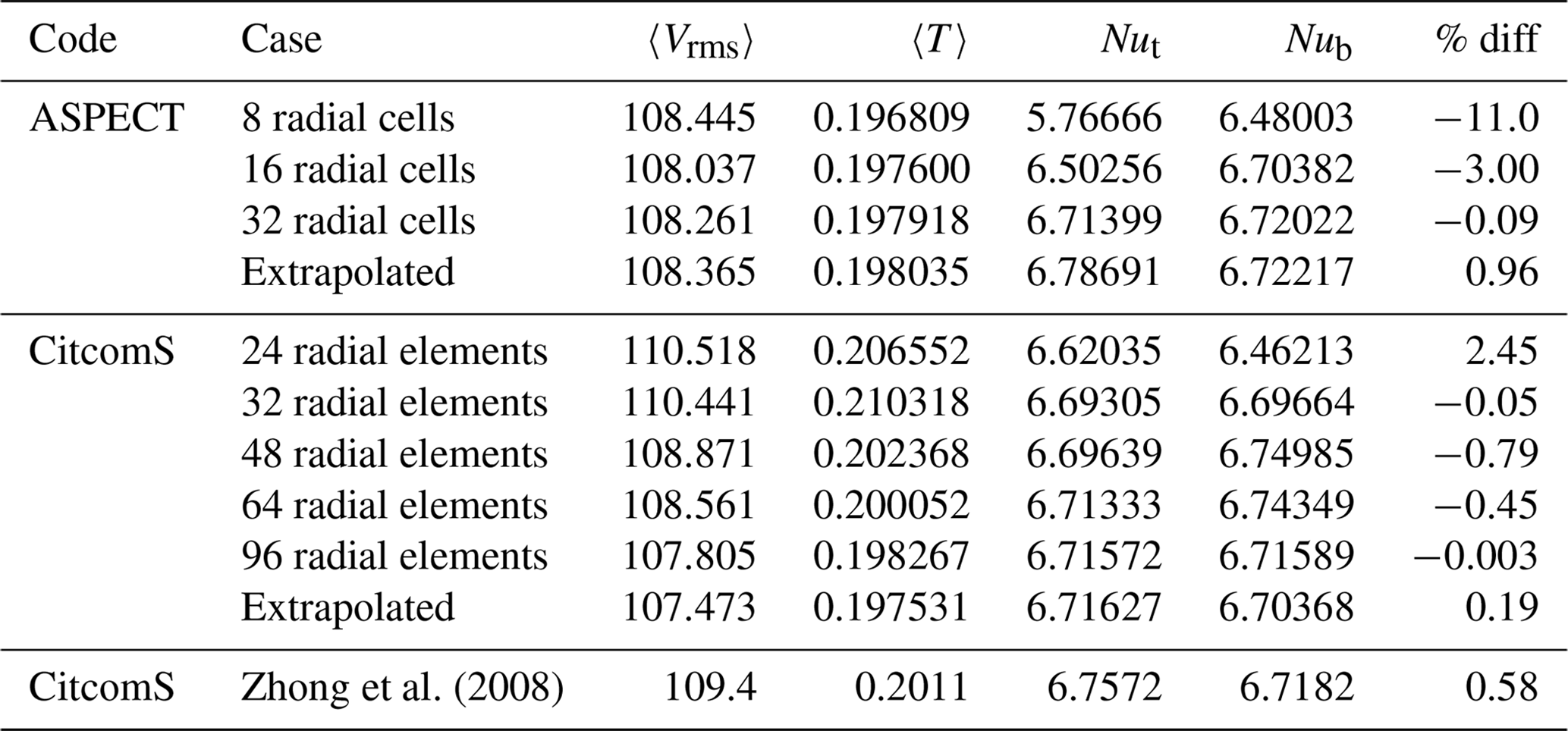
Table 10Results for Case C3 on all meshes tested. The column labeled “% diff” represents the percent difference between top and bottom Nusselt numbers for each case. A Richardson extrapolation was applied to the different data sets to estimate the values of a theoretical mesh of infinite refinement.
3.2.2 The 3-D results for the weakly temperature-dependent viscosity cases: C2 and C3
Case C2 (Fig. 2e) has a weakly temperature-dependent viscosity, Δη=10 (Table 2). The top and bottom Nusselt numbers converge within 0.6 % for CitcomS and within 0.1 % for ASPECT. The agreement between Nusselt numbers is markedly different for the two codes in this case (Table 9). ASPECT results at 8-cell radial resolution show differences of 10 %, significantly higher than any previous case. However, increased resolution caused a dramatic convergence, allowing for agreement as good as all previous cases reported. CitcomS results did not approach the difference observed with ASPECT on the most coarse meshes, although the 24-radial-element and 323-radial-element meshes produced values that both did not match the pattern of convergence of the more refined meshes.
The ASPECT results show well-behaved convergence for all parameters calculated (Fig. 9). The rms velocity and temperature show very little change with increased resolution. Both Nusselt numbers show more change between resolutions, with the top Nusselt number changing the most, but both numbers show very stable convergence. CitcomS shows more difficulty with this case. Results for all values show an initial increase through the coarse meshes which then begins to decrease and converge. All values show a similar change, with the bottom Nusselt number changing the least. The temperature of the CitcomS runs also returns to a similar level to that produced by the coarse refined meshes. Despite this difficulty, radially averaged plots show that the solutions of the most refined meshes still agree to a high degree between CitcomS and ASPECT (Fig. 3).
Case C3 (Fig. 2f) has a slightly stronger temperature-dependent viscosity, Δη=30. Top and bottom Nusselt numbers converge to within 0.1 % for both CitcomS and ASPECT on both meshes. As in Case C2, ASPECT results for Case C3 at 8-radial-cell resolution have a surprisingly high difference between Nusselt numbers. But, once again, increased resolution strongly increases convergence. By the 32-radial-cell resolution, convergence is better resolved than Case C1 at constant viscosity. CitcomS seems to have less trouble with Case C3 than Case C2.
Convergence for both codes is good for all parameters tested (Fig. 10). Nusselt numbers at the top and bottom especially show very high agreement between CitcomS and ASPECT, as well as the numbers reported by Zhong et al. (2008). Average temperature shows different time series evolution between the two codes, but convergence is still achieved as resolution increases. The rms velocity shows the largest difference between the codes with increased resolution. Values from CitcomS and ASPECT are on different tracks, and while they do show overall convergence, it is not to the same degree as the other parameters. As with the previous C cases, radially averaged plots show that the most well-resolved meshes produce highly similar solutions between CitcomS and ASPECT (Fig. 3).
We note excellent agreement in the rms velocity, mean temperature, and top and bottom Nusselt number between the two codes on the most refined meshes. If we take the difference between the top and bottom Nusselt numbers as a measure of the accuracy of the solution, which should be zero for incompressible flow at steady state, the 16-radial-cell ASPECT mesh results are already within 1 % for the A cases. CitcomS requires a 32-radial-element mesh to achieve the less than 1 % difference between the top and bottom Nusselt numbers for Cases A1 and A3; Case A7 requires a 48-radial-element mesh.
For the higher-Rayleigh-number C cases, both codes need more refined meshes to achieve a 1 % difference between the top and bottom Nusselt numbers. For ASPECT a 32-radial-cell mesh is needed, while for CitcomS a 48-radial-cell mesh is needed. We note that CitcomS shows some outlier cases where coarser meshes have unusually small percent differences between top and bottom Nusselt numbers. We use the overall pattern of convergence between the various mesh resolutions as a more accurate measure of the necessary refinement.
In general, globally averaged diagnostics from both codes at the highest mesh resolutions tested agree to within 0.6 %, and the Richardson extrapolation of the results from increasing mesh resolution agrees to within 1.0 %. Often the Richardson extrapolation agrees to within 0.5 %. ASPECT generates better-resolved solutions on coarser meshes than CitcomS, as would be expected because it uses higher-order elements. ASPECT also has several methods of improving the performance of these calculations. Adaptive refinement, both dynamically or statically through refining the boundary layers, can resolve features while reducing computational effort. This was not used in this study to facilitate similarity between the two codes. ASPECT also has a newer geometric multigrid solver (Clevenger and Heister, 2021) that can speed up computation by a factor of 3. Both of these will require further investigation and careful testing outside the scope of this current work.
Many studies use CitcomS results computed on a 64-radial-element mesh, often with limited convergence checks on more refined meshes. For the intermediate C family cases, we find that there is little difference between the 64-radial-element and 96-radial-element meshes, which generally supports the use of a 64-radial-element mesh.
Using the streamline upwind Petrov–Galerkin (SUPG) energy solver for ASPECT we find extremely good agreement between CitcomS and ASPECT results for these low to intermediate Rayleigh number calculations. Both CitcomS and ASPECT use the SUPG algorithm to solve the energy equation. For the selected cases A1, A3, and C1 we find the entropy viscosity (EV) energy solver is as good and in many cases slightly better than the SUPG solver. We caution that these calculations have Nusselt numbers that are at least a factor of 3 smaller than anticipated values for Venus or Earth.
All software used to generate these results is freely available. ASPECT is publicly available on GitHub at https://github.com/geodynamics/aspect (last access: 6 June 2023) and can be found permanently at https://doi.org/10.5281/zenodo.3924604 (Bangerth et al., 2020a). CitcomS is also publicly available on GitHub at https://github.com/geodynamics/citcoms (last access: 6 June 2023) and can be found permanently at https://doi.org/10.5281/zenodo.7271919 (Moresi et al., 2014). The data underlying this paper are made accessible through the Virginia Tech Data Repository at https://doi.org/10.7294/22803335 (Euen et al., 2023).
SDK, GTE, and SL were responsible for the initial conceptualization of this study. Software updates for use of SUPG in ASPECT were developed by TH and RG. ASPECT simulations were designed by SL. Models calculated using ASPECT were performed by GTE and SL, and models calculated using CitcomS were performed by SDK. GTE performed the data curation and formal analysis and prepared the manuscript with contributions from all co-authors.
The contact author has declared that none of the authors has any competing interests.
Publisher's note: Copernicus Publications remains neutral with regard to jurisdictional claims in published maps and institutional affiliations.
We thank the Computational Infrastructure for Geodynamics (http://geodynamics.org, last access: 6 June 2023), which is funded by the National Science Foundation under awards EAR-0949446 and EAR-1550901, administered by University of California, Davis.
Shangxin Liu was partially supported by EarthScope and GeoPRISMS programs of the National Science Foundation through the Mid-Atlantic Geophysical Integrative Collaboration (MAGIC) project (grant no. EAR-1250988). Timo Heister was partially supported by the National Science Foundation (award nos. DMS-2028346, OAC-2015848, and EAR-1925575) and by the Computational Infrastructure for Geodynamics through the National Science Foundation (award nos. EAR-0949446 and EAR-1550901). Rene Gassmöller was partially supported by the National Science Foundation (award nos. EAR-1925677 and EAR-2054605) and by the Computational Infrastructure for Geodynamics through the National Science Foundation (award nos. EAR-0949446 and EAR-1550901).
This paper was edited by Ludovic Räss and reviewed by Christian Hüttig and one anonymous referee.
Arndt, D., Bangerth, W., Blais, B., Fehling, M., Gassmöller, R., Heister,
T., Heltai, L., Köcher, U., Kronbichler, M., Maier, M., Munch, P.,
Pelteret, J.-P., Proell, S., Simon, K., Turcksin, B., Wells, D., and Zhang,
J.: The deal.II Library, Version 9.3, J. Numer.
Math., 29, 171–186, https://doi.org/10.1515/jnma-2021-0081, 2021. a
Bangerth, W., Hartmann, R., and Kanschat, G.: deal. II – A general-purpose object-oriented finite element library, ACM Transactions on Mathematical Software (TOMS), 33, 24–es, https://doi.org/10.1145/1268776.1268779, 2007. a
Bangerth, W., Dannberg, J., Gassmoeller, R., and Heister, T.: ASPECT v2.2.0 (v2.2.0), Zenodo [code], https://doi.org/10.5281/zenodo.3924604, 2020a. a, b
Bangerth, W., Dannberg, J., Gassmoeller, R., and Heister, T.: ASPECT: Advanced Solver for Problems in Earth's ConvecTion, User Manual, Figshare [data set], https://doi.org/10.6084/m9.figshare.4865333.v7, 2020b. a
Bangerth, W., Dannberg, J., Fraters, M., Gassmoeller, R., Glerum, A., Heister, T., Myhill, R., and Naliboff, J.: ASPECT: Advanced Solver for Problems in Earth's ConvecTion, User Manual, Figshare [data set], https://doi.org/10.6084/m9.figshare.4865333.v9, 2022. a, b
Baumgardner, J. R.: Three-dimensional treatment of convective flow in the Earth's mantle, J. Stat. Phys., 39, 501–511, 1985. a
Brooks, A. N. and Hughes, T. J. R.: Streamline upwind/Petrov-Galerkin formulations for convection dominated flows with particular emphasis on the incompressible Navier-Stokes equations, Comput. Meth. Appl. Mech. Eng., 32, 199–259, 1982. a
Bunge, H.-P., Richards, M. A., and Baumgardner, J. R.: Effect of depth-dependent viscosity on the planform of mantle convection, Nature, 379, 436–438, 1996. a
Burstedde, C., Stadler, G., Alisic, L., Wilcox, L. C., Tan, E., Gurnis, M., and Ghattas, O.: Large-scale adaptive mantle convection simulation, Geophys. J. Int., 192, 889–906, 2013. a
Choblet, G.: Modelling thermal convection with large viscosity gradients in one block of the “cubed sphere”, J. Comput. Phys., 205, 269–291, 2005. a
Choblet, G., Čadek, O., Couturier, F., and Dumoulin, C.: OEDIPUS: a new tool to study the dynamics of planetary interiors, Geophys. J. Int., 170, 9–30, 2007. a
Clevenger, T. C. and Heister, T.: Comparison between algebraic and matrix-free geometric multigrid for a Stokes problem on adaptive meshes with variable viscosity, Numer. Linear Algebr., 28, https://doi.org/10.1002/nla.2375, 2021. a
Davies, D. R., Davies, J. H., Bollada, P. C., Hassan, O., Morgan, K., and Nithiarasu, P.: A hierarchical mesh refinement technique for global 3-D spherical mantle convection modelling, Geosci. Model Dev., 6, 1095–1107, https://doi.org/10.5194/gmd-6-1095-2013, 2013. a
Euen, G., Liu, S., Gassmöller, R., Heister, T., and King, S.: Data associated with “A Comparison of 3-D Spherical Shell Thermal Convection results at Low to Moderate Rayleigh Number using ASPECT (version 2.2.0) and CitcomS (version 3.3.1)”, University Libraries, Virginia Tech, [data set], https://doi.org/10.7294/22803335, 2023. a
Foley, B. and Becker, T. W.: Generation of plate tectonics and mantle heterogeneity from a spherical, visco-plastic convection model, Geochem. Geophys. Geosys., 10, 8, https://doi.org/10.1029/2009GC002378, 2009. a
Glerum, A., Thieulot, C., Fraters, M., Blom, C., and Spakman, W.: Nonlinear viscoplasticity in ASPECT: benchmarking and applications to subduction, Solid Earth, 9, 267–294, https://doi.org/10.5194/se-9-267-2018, 2018. a
Guermond, J.-L., Pasquetti, R., and Popov, B.: Entropy viscosity method for nonlinear conservation laws, J. Comput. Phys., 230, 4248–4267, 2011. a
He, Y., Puckett, E. G., and Billen, M. I.: A discontinuous Galerkin method with a bound preserving limiter for the advection of non-diffusive fields in solid Earth geodynamics, Phys. Earth Planet. In., 263, 23–37, 2017. a
Heister, T., Dannberg, J., Gassmöller, R., and Bangerth, W.: High accuracy mantle convection simulation through modern numerical methods - II: realistic models and problems, Geophys. J. Int., 210, 833–851, https://doi.org/10.1093/gji/ggx195, 2017. a, b, c, d, e
Hüttig, C., Tosi, N., and Moore, W. B.: An improved formulation of the incompressible Navier–Stokes equations with variable viscosity, Phys. Earth Planet. In., 220, 11–18, https://doi.org/10.1016/j.pepi.2013.04.002, 2013. a
Kageyama, A. and Sato, T.: “Yin-Yang grid”: An overset grid in spherical geometry, Geochem. Geophys. Geosyst., 5, https://doi.org/10.1029/2004GC000734, 2004. a
King, S. D.: Pattern of lobate scarps on Mercury's surface reproduced by a model of mantle convection, Nat. Geo., 1, 229–232, https://doi.org/10.1038/ngeo152, 2008. a
King, S. D.: Venus Resurfacing Constrained by Geoid and Topography, J. Geophys. Res.-Planets, 123, 1041–1060, 2018. a
King, S. D., Raefsky, D. A., and Hager, B. H.: ConMan: vectorizing a finite element code for incompressible two-dimensional convection in the Earth's mantle, Phys. Earth Planet. Inter., 59, 195–207, 1990. a
Kronbichler, M., Heister, T., and Bangerth, W.: High accuracy mantle convection simulation through modern numerical methods, Geophys. J. Int., 191, 12–29, https://doi.org/10.1111/j.1365-246X.2012.05609.x, 2012. a, b, c, d, e, f
Liu, S. and King, S. D.: A benchmark study of incompressible Stokes flow in a 3-D spherical shell using ASPECT, Geophys. J. Int., 217, 650–667, 2019. a
Liu, X. and Zhong, S.: The long-wavelength geoid from three-dimensional spherical models of thermal and thermochemical mantle convection, J. Geophys. Res.-Sol. Ea., 120, 4572–4596, 2015. a
McNamara, A. and Zhong, S.: Thermochemical structures within a spherical mantle: Superplumes or piles?, J. Geophys. Res.-Sol. Ea., 109, B07402, https://doi.org/10.1029/2003JB002847, 2004. a, b
McNamara, A. K. and Zhong, S.: Thermochemical Piles Under Africa and the Pacific, Nature, 437, 1136–1139, 2005. a
Moresi, L., Zhong, S., Han, L., Conrad, C., Tan, E., Gurnis, M., Choi, E., Thoutireddy, P., Manea, V., McNamara, A., Becker, T., Leng, W., and Armendariz, L.: CitcomS v3.3.1 (v3.3.1), Zenodo [code], https://doi.org/10.5281/zenodo.7271920, 2014. a, b
Puckett, E. G., Turcotte, D. L., He, Y., Lokavarapu, H., Robey, J. M., and Kellogg, L. H.: New numerical approaches for modeling thermochemical convection in a compositionally stratified fluid, Phys. Earth Planet. In., 276, 10–35, 2017. a
Ratcliff, J. T., Schubert, G., and Zebib, A.: Steady tetrahedral and cubic patterns of spherical shell convection with temperature-dependent viscosity, J. Geophys. Res.-Sol. Ea., 101, 25473–25484, 1996. a, b
Roberts, J. H. and Zhong, S.: Plume-induced topography and geoid anomalies and their implications for the Tharsis rise on Mars, J. Geophys. Res.-Planets, 109, E3, https://doi.org/10.1029/2003JE002226, 2004. a
Schubert, G., Turcotte, D. L., and Olson, P.: Mantle convection in the Earth and planets, Cambridge University Press, https://doi.org/10.1017/CBO9780511612879, 2001. a
Sekhar, P. and King, S. D.: 3D spherical models of Martian mantle convection constrained by melting history, Earth Planet. Sci. Lett., 388, 27–37, https://doi.org/10.1016/j.epsl.2013.11.047, 2014. a
Stadler, G., Gurnis, M., Burstedde, C., Wilcox, L. C., Alisic, L., and Ghattas, O.: The Dynamics of Plate Tectonics and Mantle Flow: From Local to Global Scales, Science, 329, 1033–1038, 2010. a
Stemmer, K., Harder, H., and Hansen, U.: A new method to simulate convection with strongly temperature-and pressure-dependent viscosity in a spherical shell: Applications to the Earth's mantle, Phys. Earth Planet. In., 157, 223–249, 2006. a, b
Tackley, P. J.: Modelling compressible mantle convection with large viscosity contrasts in a three-dimensional spherical shell using the yin-yang grid, Phys. Earth Planet. In., 171, 7–18, 2008. a
Tan, E., Gurnis, M., and Han, L.: Slabs in the lower mantle and their modulation of plume formation, Geochem. Geophys. Geosys., 3, 1–24, https://doi.org/10.1029/2001GC000238, 2002. a
Tan, E., Choi, E., Thoutireddy, P., Gurnis, M., and Aivazis, M.: GeoFramework: Coupling multiple models of mantle convection within a computational framework, Geochem. Geophys. Geosyst., 7, Q06001, https://doi.org/10.1029/2005GC001155, 2006. a, b, c, d
Thieulot, C.: Analytical solution for viscous incompressible Stokes flow in a spherical shell, Solid Earth, 8, 1181–1191, https://doi.org/10.5194/se-8-1181-2017, 2017. a
Tosi, N., Stein, C., Noack, L., Hüttig, C., Maierová, P., Samuel, H., Davies, D. R., Wilson, C. R., Kramer, S. C., Thieulot, C., Glerum, A., Fraters, M., Spakman, W., Rozel, A., and Tackley, P. J.: A community benchmark for viscoplastic thermal convection in a 2-D square box, Geochem. Geophys. Geosyst., 16, 2175–2196, 2015. a
Yoshida, M. and Kageyama, A.: Application of the Yin-Yang grid to a thermal convection of a Boussinesq fluid with infinite Prandtl number in a three-dimensional spherical shell, Geophys. Res. Lett., 31, 12, https://doi.org/10.1029/2004GL019970, 2004. a, b
Zhong, S.: Constraints on thermochemical convection of the mantle from plume heat flux, plume excess temperature and upper mantle temperature, J. Geophys. Res., 111, B4, https://doi.org/10.1029/2005JB003972, 2006. a
Zhong, S., Zuber, M., Moresi, L., and Gurnis, M.: Role of temperature-dependent viscosity and surface plates in spherical shell models of mantle convection, J. Geophys. Res.-Sol. Ea., 105, 11063–11082, https://doi.org/10.1029/2000JB900003, 2000. a, b, c, d, e
Zhong, S., McNamara, A., Tan, E., Moresi, L., and Gurnis, M.: A benchmark study on mantle convection in a 3-D spherical shell using CitcomS, Geochem. Geophys. Geosyst., 9, 10, https://doi.org/10.1029/2008GC002048, 2008. a, b, c, d, e, f, g, h, i, j, k, l, m, n, o, p, q, r, s, t, u, v, w, x, y, z, aa, ab, ac, ad, ae, af, ag, ah, ai, aj, ak, al, am, an, ao