Halogen chemistry in volcanic plumes: a 1D framework based on MOCAGE 1D (version R1.18.1) preparing 3D global chemistry modelling

HBr emissions from volcanoes lead rapidly to the formation of BrO within volcanic plumes and have an impact on tropospheric chemistry, at least at the local and regional scales. The motivation of this paper is to prepare a framework for further 3D modelling of volcanic halogen emissions in order to determine their fate within the volcanic plume and then in the atmosphere at the regional and global scales. The main aim is to evaluate the ability of the model to produce a realistic partitioning of bromine species within a grid box size typical of MOCAGE (Model Of atmospheric Chemistry At larGE scale) 3D (0.5^∘ × 0.5^∘). This work is based on a 1D single-column configuration of the global chemistry-transport model MOCAGE that has low enough computational cost to allow us to perform a large set of sensitivity simulations. This paper uses the emissions from the Mount Etna eruption on 10 May 2008. Several reactions are added to MOCAGE to represent the volcanic plume halogen chemistry. A simple plume parameterisation is also implemented and tested. The use of this parameterisation tends to only slightly limit the efficiency of BrO net production. Both simulations with and without the parameterisation give results for the partitioning of the bromine species, of ozone depletion and of the $\mathrm{BrO}/{\mathrm{SO}}_{\mathrm{2}}$ ratio that are consistent with previous studies.

A series of test experiments were performed to evaluate the sensitivity of the results to the composition of the emissions (primary sulfate aerosols, Br radical and NO) and to the effective radius assumed for the volcanic sulfate aerosols. Simulations show that the plume chemistry is sensitive to all these parameters. We also find that the maximum altitude of the eruption changes the BrO production, which is linked to the vertical variability of the concentrations of oxidants in the background air. These sensitivity tests display changes in the bromine chemistry cycles that are generally at least as important as the plume parameterisation. Overall, the version of the MOCAGE chemistry developed for this study is suitable to produce the expected halogen chemistry in volcanic plumes during daytime and night-time.

1 Introduction

Volcanoes are an important source of gases injected into the atmosphere. In addition to the main gaseous emissions of water vapour, CO₂ and SO₂, volcanoes also emit inorganic halogen compounds mainly as HCl, HF and HBr (Gerlach, 2004). HF is very unreactive in the context of gas-phase tropospheric chemistry, while HCl and HBr are both reactive species in this environment. Bromine and to a much lesser extent chlorine induce tropospheric ozone loss at the global scale and subsequent OH loss, therefore affecting the tropospheric oxidising capacity (e.g. Saiz-Lopez and von Glasow, 2012; Simpson et al., 2015; Sherwen et al., 2016). But the hydrogen halides (HX, with X = Cl, Br, F, I) have a high effective solubility, meaning that HCl and HBr emitted by volcanoes are scavenged onto the Earth's surface by wet deposition within a few hours to a few days. Consequently, their direct impact on the air composition in the troposphere was expected to be local and weak.

However, this point of view was challenged when Bobrowski et al. (2003) observed bromine monoxide (BrO) in the plume of the Soufrière Hills volcano, Montserrat. After this first observation, BrO has been measured in many other volcanic plumes (e.g. Oppenheimer et al., 2006; Theys et al., 2009; Boichu et al., 2011; Bobrowski and Giuffrida, 2012; Hörmann et al., 2013, Kern and Lyons, 2018; Roberts, 2018; Seo et al., 2019). The detection of volcanic BrO is significant because unlike HCl and HBr, BrO is not water soluble. Its observed presence several kilometres downwind also indicates the occurrence of reactive halogen cycling in volcanic plumes from HBr. This implies a longer atmospheric residence time for volcanic bromine and therefore opens conditions for regional- to global-scale impacts on tropospheric chemical composition. The purpose of this study is to prepare a framework for simulating the atmospheric chemistry of volcanic halogen emissions in a global model, in order to determine their fate in the volcanic plume, and ultimately at the regional and global scales.

Regarding the source of volcanic BrO, Gerlach (2004) first suggested that BrO is not directly emitted by volcanoes and that chemical reactions in the high-temperature mixture of air and magmatic gases, immediately following emission, generate radicals that could potentially form BrO further downwind. A variety of such mixtures, depending on varying proportions of air and magmatic gases, were later studied by Martin et al. (2006). However, this near-vent source of radicals (Br, Cl, NO, OH) cannot itself explain the occurrence of BrO further downwind. Studies of the multi-phase plume atmospheric chemistry (e.g. Oppenheimer et al., 2006; Bobrowski et al., 2007; Roberts et al., 2009, 2014; von Glasow et al., 2009; Kelly et al., 2013; Surl et al., 2015, 2021; Jourdain et al., 2016) have highlighted autocatalytic reaction cycles as the key mechanism for BrO production in later stages of volcanic plume evolution, at temperatures closer to that of ambient air. Rapid bromine cycling can also lead to the formation of reactive chlorine (e.g. Jourdain et al., 2016; Roberts et al., 2018). The basis for BrO formation is halogen heterogeneous chemistry occurring in the presence of acidic aerosol. This process is similar to the so-called “bromine explosion” (Platt and Lehrer, 1997; Wennberg, 1999) that was identified in the tropospheric polar region. The net reaction of the cycle consists of a rapid and strong production of BrO from HBr volcanic emissions. Ozone molecules are depleted during this cycle. The environment where the chemical cycle takes place needs to have a pH < 7 (Fickert et al., 1999). This pH condition is readily achieved in a volcanic plume containing acid gases and sulfate aerosols. Moreover, the “at source” or primary sulfate aerosols present in the volcanic source promote heterogeneous chemistry to form BrO. Model sensitivity tests (e.g. Roberts et al., 2014) find that high-temperature radicals (Br, Cl, NO, OH) in the model initialisation act to kick-start the onset of the bromine explosion. Numerical atmospheric models (e.g. Bobrowski et al., 2007; Roberts et al., 2009) containing the bromine explosion mechanism and initialised with a volcanic emission that includes HBr, HCl, SO₂, primary sulfate and a representation of the high-temperature radicals (e.g. Br, Cl, NO, OH) were able to reproduce the BrO observed downwind from volcanoes. More details on the current knowledge on bromine in volcanic plumes are given in the review by Gutmann et al. (2018).

Most previous numerical modelling studies describing halogen chemistry in volcanic plumes (Bobrowski et al., 2007; Roberts et al., 2009, 2014; von Glasow, 2010; Kelly et al., 2013; Surl et al., 2015) focused on the local volcanic chemistry within the plume in a zero- or one-dimensional Lagrangian framework. The same thermodynamic equilibrium model was used in the initialisation of the atmospheric chemistry models in most of these studies (Bobrowski et al., 2007; Roberts et al., 2009; von Glasow, 2010; Surl et al., 2015) to describe the high-temperature mixtures of air and volcanic gases. This model is the HSC Chemistry software (Martin et al., 2006, 2009) that, similar to the abovementioned work of Gerlach (2004), predicts the high-temperature formation of many species other than the raw volcanic emissions, in particular halogen radicals and oxidants. The plume/atmospheric chemistry modelling studies initialised using HSC outputs show a rapid increase in BrO within the plume in the few minutes after an emission, consistent with plume observations. However, recent studies (e.g. Aiuppa et al., 2007a; Martin et al., 2012; Roberts et al., 2019) have shown that the assumption of thermodynamic equilibrium used in HSC is not realistic, in particular for NO_x and H₂S. New kinetics-based models of the hot plume chemistry are in development (Roberts et al., 2019) but do not yet contain halogens.

Most previous studies on the volcanic plume chemistry were at the plume scale over only a few hours from emission. However, bromine emissions can be transported within the plume at regional scales (Jourdain et al., 2016; Narivelo et al., 2023). It is therefore also interesting to study their effect at larger time and spatial scales. For this, it is possible to use 3D regional or global atmospheric chemistry models. Jourdain et al. (2016) studied an episode of extreme passive degassing of Ambrym (Vanuatu) with the coupled meteorology–chemistry mesoscale model C-CCATT-BRAMS (Longo et al., 2013) with four nested grids from 50 km (regional grid) down to 0.5 km (close to vent grid) horizontal resolutions. Their results confirmed the influence of volcanic halogen emissions at the local and regional scales (several thousand kilometres from the volcano) on the oxidising capacity of the troposphere. In particular, they showed an impact on methane lifetime. Recently, Surl et al. (2021) studied a plume from Mt Etna passive degassing based on 3D model simulations with the WRF-Chem model at ∼ 1 km resolution compared to aircraft observations of ozone and ground-based remote sensing of BrO. The study focused on the region from the volcano to tens of kilometres downwind. Surl et al. (2021) show that the wind speed and the time of the day have non-linear effects on the $\mathrm{BrO}/{\mathrm{SO}}_{\mathrm{2}}$ ratio that characterises the BrO production efficiency. They also highlight the impacts of the halogen chemistry on reactive nitrogen and on HO_x with the consequence of slower secondary sulfate aerosol formation. From sensitivity simulations, they confirmed the importance of the composition of the emission source resulting from high-temperature processes, in particular Br radicals, for the rapid BrO production in the plume. Both of these 3D model studies used nested grids to simulate plume chemistry in a regional model at high spatial resolution (km) over a limited area.

A step further is to study this influence from the regional to the global scales based on 3D chemistry-transport models (CTMs). Because of the typical coarse resolution of such models (typically from ∼ 2 to ∼ 0.1^∘ , or hundreds to tens of kilometres), there is no possibility to represent the fine-scale plume chemistry in global CTMs. Processes occurring at subgrid scales are generally represented via parameterisations in atmospheric models, giving a better description of the phenomenon studied in the case of plumes (e.g. Karamchandani et al., 2002; Cariolle et al., 2009). Therefore, a parameterisation might be required to properly represent the rapid chemistry processing within the volcanic plumes in their early stages when they contain high concentrations of sulfur and halogens. This was one of the aims of the study of Grellier et al. (2014) that developed and tested in a one-dimensional (vertical column) modelling framework a simple subgrid-scale parameterisation of halogen plume chemistry at 0.5 and 2^∘ horizontal resolutions. The second and main aim of Grellier et al. (2014) was to evaluate the implementation of the volcanic bromine chemistry in MOCAGE (Model Of atmospheric Chemistry At larGE scale). This study was not successful because of its simplified representation of bromine chemistry, in particular the lack of Br₂ species.

The present paper is an extended version of Grellier at al. (2014) with major updates but with the same motivation of preparing from 1D simulations the implementation and use of volcanic halogen chemistry in the 3D global/regional CTM MOCAGE. The first and main objective is to evaluate if the halogen chemistry developed in MOCAGE and based on previous studies is able to produce a realistic bromine partition at a typical MOCAGE 3D model box size. For this, the volcanic chemistry scheme was updated, in particular by the introduction of Br₂ species. The second and secondary objective is to address the effect on the bromine explosion of the assumption that the chemical species are homogeneously distributed within each model grid box while the typical size of a volcanic plume at its early stage is much smaller than the MOCAGE horizontal resolution. This part of the study derives from the plume parameterisation approach of Grellier et al. (2014). Here we expand this approach to represent more realistically the chemistry at the plume scale. Because of the low computing cost of the 1D simulations, we performed a set of sensitivity tests on the impact of different parameters on the bromine cycle within the plume. This includes the choice of the composition of the volcanic emissions used as input. As discussed above, there is not a full understanding of the processes occurring when magmatic air first mixes with atmospheric air at high temperature. Previous studies showed that the choice of this composition is important at fine-scale resolutions since it can lead to large changes in the time evolution of the bromine partition (Roberts et al., 2009, 2014; Jourdain et al., 2016; Surl et al., 2021). Here, we will investigate the impact of the composition of the emissions at a coarser grid size that is typical of the 3D MOCAGE simulations and compare the results to previous studies. We use the 1D MOCAGE modelling framework as a test bed to analyse the impact of the time of the day, the size of the volcanic sulfate aerosols and the altitude of the emissions on the bromine explosion efficiency.

In Sect. 2, a description of the volcanic eruption studied in this paper is given. Then the numerical model, 1D version of MOCAGE, is presented in Sect. 3, including the upgrades needed to represent volcanic halogen chemistry. The simulations are described in Sect. 4. Section 5 presents the analysis of the results of the simulations. Conclusions are given in Sect. 6.

2 Case study: the Etna eruption of 10 May 2008

The philosophy of the paper is to make a plausible case study to test the volcanic chemistry scheme implemented in the 1D model and not a detailed analysis of the eruption. To try to run the model with realistic conditions, we picked the particular Etna eruption of 10 May 2008 because its SO₂ emission flux and height have been estimated in a previous study and we have information from observations on the magmatic gas composition for halogens.

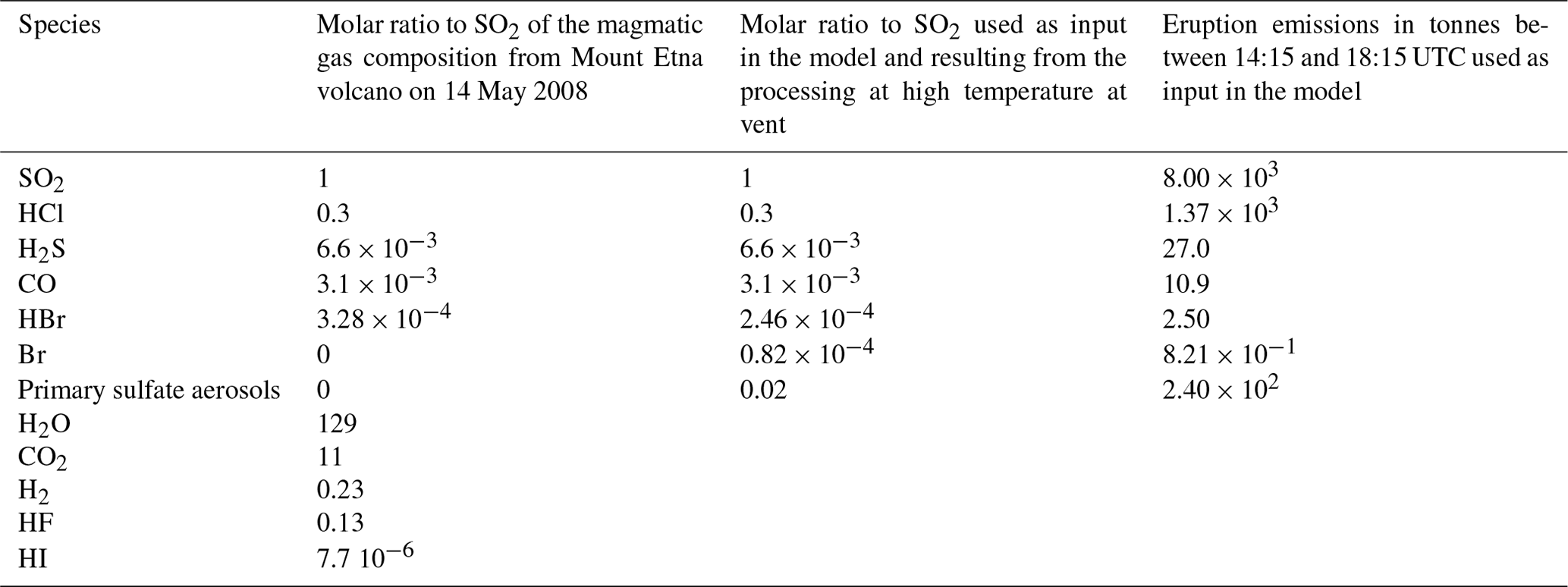
Table 1 Composition of the volcanic emissions: magmatic gas emissions and emissions used as input for the MOCAGE 1D model for the reference experiment N.Ref. In the N.Ref simulation, the primary sulfate aerosols are uniformly distributed with an effective radius of 0.3 µm (see explanation and justification in Sect. 4.1).

2.1 General description

Mount Etna is the most active volcano in Europe and among the largest point sources of volcanic volatiles on the planet (Aiuppa et al., 2008). Gases and aerosols and possibly volcanic ash are continually emitted by the craters by passive or explosive degassing. Four craters are currently hosted on the volcano summit; the volcano itself has a total surface area of 1200 km², and the mean altitude of the volcanic plateau is at an altitude of 3300 m.

This study focuses on the eruption of Mount Etna that occurred on 10 May 2008 (see Bonaccorso et al., 2011, for more information about this eruptive event). There are two reasons behind the choice of this volcanic eruption: (1) Mount Etna is one of the largest known emission sources of halogens (Aiuppa et al., 2005) and (2) the Mount Etna volcano is also continuously and extensively monitored by INGV (Istituto Nazionale di Geofisica e Vulcanologia), including emission flux estimation and gas composition needed for the model. In addition, satellite estimations of BrO and SO₂ of the plume are available on 11 May and have been used in addition to the literature to evaluate if MOCAGE 1D simulations give plausible values.

The eruption on 10 May 2008 that we study started at 14:15 UTC and lasted until 18:15 UTC (from monitoring reports of INGV Osservatorio Etneo; available at https://www.ct.ingv.it, last access: 4 April 2022). The eruptive cloud was injected from the top of Mount Etna 3300 m up to about 8500 m in altitude above mean sea level (Bonaccorso et al., 2011). The time-averaged SO₂ daily release on the day of the eruption was estimated to be 10 000 t, which is obtained by averaging results of car traverses made with an Ocean Optics USB2000+ spectrometer and a differential optical absorption spectroscopy (DOAS) retrieval technique. During May 2008, non-eruptive emissions from the volcano contributed an average of 2000 t of SO₂ per day (from monitoring reports of INGV Osservatorio Etneo; available at https://www.ct.ingv.it, last access: 4 April 2022 and from Guiseppe Salerno, personal communication, 2013).

2.2 Gas composition of the volcanic emissions

The composition of Mount Etna plumes has extensively been characterised before this case study by both in situ (e.g. Aiuppa et al., 2007b, 2008) and remote sensing (Allard et al., 2005) techniques. These studies have shown that, for volcanic gas emissions in general (Oppenheimer, 2003), Etna's magmatic volatiles are dominated by H₂O, CO₂ and SO₂, in proportions varying both in time (depending on activity state) and location (e.g. from crater to crater). Etna's magmatic gases also include smaller but significant amounts of halogen species (HCl, HF and HBr).

Bromine emissions can be satisfactorily derived by in situ direct sampling of both fumaroles (Gerlach, 2004) and plumes (Aiuppa et al., 2005), but both techniques are not viable measurement strategies in eruptive plumes due to the inherent risks for operators. We here therefore use the magmatic gas composition for the Etna's passive plume (Table 1) derived on 14 May 2008 by a combination of techniques (MultiGAS for H₂O, CO₂, and SO₂ and filter packs for halogens; see Aiuppa et al., 2005, 2007b, 2008, for analytical details). Note that previous modelling case studies of real volcanic emissions have also set the composition of the magmatic gas from in situ measurements (Jourdain et al., 2016; Surl et al., 2021). Here, the in situ data gathered on 14 May 2008 are used as an analogue for 10 May 2008 eruptive plume composition. This assumption is motivated by the hydraulic continuity between the central craters (where passive emissions concentrate) and the southeast crater (the eruptive vent), for which there is plenty of seismic (Patanè et al., 2003), gas (Aiuppa et al., 2010) and infrasonic (Marchetti et al., 2009) evidence. Moreover, since the aim of the paper is to use this case study as a test bed for plume chemistry modelling and not to make a detailed analysis of the eruption, the gas composition on 14 May 2008 is realistic enough to be used here.

3 Model description

The numerical model used for the simulations is a 1D configuration, called hereafter MOCAGE 1D, of the three-dimensional global and regional chemistry-transport model MOCAGE (Model Of atmospheric Chemistry At larGE scale; Josse et al., 2004; Cussac et al., 2020; Lamotte et al., 2021). MOCAGE is developed by Météo-France to simulate air composition for research (e.g. Lacressonnière et al., 2014) and operational applications (e.g. Marécal et al., 2015). This 1D configuration allows us to make a large set of sensitivity tests on the many parameters that can modify the chemical processing within a volcanic plume. It does not intend to reproduce the exact chemical evolution focusing on local scale at the very early stage (< 1 h) within the volcanic plume as done in previous studies (e.g. Roberts et al., 2009).

The 1D configuration corresponds here to the vertical column above the emission source (i.e. above Etna's location). It assumes no transport horizontally and vertically (unlike the 3D version). Thus, the boxes constituting the vertical column are not interacting with each other and can be considered as an ensemble of independently piled 0D boxes. The only connection between the boxes is through photolysis rates. Because there is no horizontal transport in MOCAGE 1D, there is no exchange of air at the outside boundaries of the considered column. Even if in reality there is mixing of the volcanic plumes with background air at a scale larger than the model grid box (here 0.5^∘ longitude × 0.5^∘ latitude), this becomes significant only after several hours up to 1–2 d. Since the MOCAGE 1D simulations are run over a maximum of 20 h, this setup is thus reasonable to study the plume chemistry and to address its sensitivity to different parameters. The possible impact of neglecting this effect is taken into account in the analysis of the results.

Like in the 3D version of MOCAGE (called hereafter MOCAGE 3D), the vertical resolution of the 1D column is divided into 47 levels from the ground up to 5 hPa. It uses the sigma hybrid coordinate: close to the surface, the levels follow the orography while the highest levels follow isobars. The interval between levels increases with altitude with 7 levels within the planetary boundary layer, 20 in the free troposphere and 20 in the stratosphere.

The 1D configuration of MOCAGE is designed so that the chemistry model developed for volcanic emissions can be seamlessly inserted into MOCAGE 3D. Thus, the injection of the emitted gases during the eruption is done as in MOCAGE 3D by adding volcanic gas amounts to the background air in the grid box containing the volcano vent and at the model levels impacted by the volcanic plume. For eruptions, the emissions are spread from the volcano crater altitude to the top height of the plume following an “umbrella” profile as in Lamotte et al. (2021), with an injection of 75 % of the emissions in the top third of the plume. This represents the fact that most of the mass emitted during an eruption is in the top part of the plume.

The chemical reactions represented in MOCAGE 1D start with those in MOCAGE 3D, i.e. including both the tropospheric and stratospheric chemistry, but with the addition of several reactions necessary to model the bromine explosion in volcanic plumes. The standard version of the model uses the RACMOBUS chemistry scheme, which is a merger of the REPROBUS stratospheric scheme (Lefèvre et al., 1994) with the RACM tropospheric chemistry scheme (Stockwell et al., 1997), completed with the sulfur cycle (Ménégoz et al., 2009; Guth et al., 2016) and peroxyacetylnitrate (PAN) photolysis. RACMOBUS is valid for remote to polluted conditions and from the Earth's surface up to the stratosphere. Altogether, the original version of the model contains 112 species with 316 gaseous reactions and 54 photolysis applied in both the troposphere and the stratosphere, as well as 9 heterogeneous reactions only applied in the stratosphere. The chemical solver is based on a semi-implicit Euler-backward method.

This scheme has been extended to represent the bromine explosion cycle. This cycle is described in detail for instance in Oppenheimer et al. (2006), Platt and Hönninger (2003), Bobrowski et al. (2007), or Roberts et al. (2009), and its main reactions are listed below:

$$\begin{array}{}\text{(R1)}& {\displaystyle }\mathrm{HBr}+\mathrm{OH}\to \mathrm{Br}+{\mathrm{H}}_{\mathrm{2}}\mathrm{O},\text{(R2)}& {\displaystyle }\mathrm{Br}+{\mathrm{O}}_{\mathrm{3}}\to \mathrm{BrO}+{\mathrm{O}}_{\mathrm{2}},\text{(R3)}& {\displaystyle }\mathrm{BrO}+{\mathrm{HO}}_{\mathrm{2}}\to \mathrm{HOBr}+{\mathrm{O}}_{\mathrm{2}},\text{(R4)}& {\displaystyle }\mathrm{BrO}+{\mathrm{NO}}_{\mathrm{2}}\to \mathrm{BrO}{\mathrm{NO}}_{\mathrm{2}},\end{array}$$

$$\begin{array}{}\text{(R5a)}& {\displaystyle }\mathrm{HOBr}+\mathrm{HBr}\left(\text{sulfate aerosol}\right)\to {\mathrm{Br}}_{\mathrm{2}}+{\mathrm{H}}_{\mathrm{2}}\mathrm{O},\text{(R5b)}& {\displaystyle }\mathrm{HOBr}+\mathrm{HCl}\left(\text{sulfate aerosol}\right)\to \mathrm{BrCl}+{\mathrm{H}}_{\mathrm{2}}\mathrm{O},\end{array}$$

$$\begin{array}{}\text{(R6)}& {\displaystyle }{\mathrm{BrONO}}_{\mathrm{2}}+{\mathrm{H}}_{\mathrm{2}}\mathrm{O}\left(\text{sulfate aerosol}\right)\to \mathrm{HOBr}+{\mathrm{HNO}}_{\mathrm{3}},\text{(R7)}& {\displaystyle }{\mathrm{Br}}_{\mathrm{2}}+h\mathit{\nu }\to \mathrm{2}\mathrm{Br},\text{(R8)}& {\displaystyle }\mathrm{BrCl}+h\mathit{\nu }\to \mathrm{Br}+\mathrm{Cl},\text{(R9)}& {\displaystyle }\mathrm{Br}+{\mathrm{HO}}_{\mathrm{2}}\to \mathrm{HBr}+{\mathrm{O}}_{\mathrm{2}},\text{(R10)}& {\displaystyle }\mathrm{BrO}+\mathrm{BrO}\to \mathrm{2}\mathrm{Br}+{\mathrm{O}}_{\mathrm{2}}.\end{array}$$

The notation “HBr(sulfate aerosol)” (respectively “HCl(sulfate aerosol)”) means that HOBr reacts heterogeneously with HBr (respectively HCl) in sulfate aerosols. Reaction (R6) corresponds to BrONO₂ hydrolysis.

This cycle leads to the autocatalytic BrO formation summarised below:

$$\begin{array}{}\text{(R11)}& {\displaystyle }\begin{array}{rl}\mathrm{BrO}+{\mathrm{HO}}_{\mathrm{2}}+\mathrm{HBr}& \left(\text{sulfate aerosol}\right)+\mathrm{2}{\mathrm{O}}_{\mathrm{3}}\\ & \to \mathrm{2}\mathrm{BrO}+\mathrm{3}{\mathrm{O}}_{\mathrm{2}}+{\mathrm{H}}_{\mathrm{2}}\mathrm{O},\end{array}\text{(R12)}& {\displaystyle }\begin{array}{rl}\mathrm{BrO}+{\mathrm{NO}}_{\mathrm{2}}+\mathrm{HBr}& \left(\text{sulfate aerosol}\right)+\mathrm{2}{\mathrm{O}}_{\mathrm{3}}\\ & \to \mathrm{2}\mathrm{BrO}+\mathrm{3}{\mathrm{O}}_{\mathrm{2}}+{\mathrm{HNO}}_{\mathrm{3}}.\end{array}\end{array}$$

Volcanic emissions contain halogen species and in particular HBr that provide the bromine atoms (Reaction R1) needed for the cycle to produce BrO. To simulate the bromine explosion cycle (Reactions R1 to R10) which corresponds to the very rapid conversion of HBr that is emitted from the volcano in reactive species (BrO in the first place), we have modified the halogen chemistry scheme in MOCAGE, originally designed for stratospheric chemistry only. In Grellier et al. (2014), Br₂ was assumed to be converted into Br instantaneously. With this assumption being only possibly valid during daytime because of Br₂ photolysis, the results of Grellier et al. (2014) simulations were not realistic at night-time. Here we introduced Br₂ as a new species and its photolysis (Reaction R7) and gas-phase reaction with OH. Additionally, we included the three heterogeneous Reactions (R5a), (R5b), and (R6) and six halogen gaseous reactions following Surl et al. (2021). The Supplement gives the list of the halogen species and reactions present in the updated version of MOCAGE chemistry and details on the calculation of the heterogeneous reactions.

4 Setup of the simulations

A large set of 1D simulations was run in different conditions using the Etna case study as a test bed to assess the model ability to produce BrO from HBr volcanic emissions, the impact of using an expanded version of the subgrid-scale parameterisation of Grellier et al. (2014) and the sensitivity of the bromine explosion to several parameters.

4.1 General model setup and description of the reference simulations

Each 1D simulation calculates the chemical concentrations of all species in the vertical levels of the model. The horizontal box size chosen is 0.5^∘ (longitude) × 0.5^∘ (latitude) resolution (∼ 44 × ∼ 55 km at the location of Mt Etna), because it is an intermediate horizontal resolution used both for global and regional studies with MOCAGE. The initial conditions of the chemical species of all simulations are the same. They correspond to the 1D profile of the species concentrations on 10 May 2008 at 14:00 UTC, extracted from the grid box that contains Mt Etna, in a 3D MOCAGE global simulation at 0.5^∘ × 0.5^∘ resolution. In the 1D simulation, we set to zero the concentrations for the inorganic chlorine and bromine species in the troposphere. This is done because in the standard version of MOCAGE 3D that is used for the initial conditions, the halogen inorganic species are only used to represent stratospheric chemistry, and their background concentrations in the troposphere cannot be considered to be reliable. Furthermore, the inorganic halogen concentrations are dominated by the injection of the volcanic eruption on the scale of the study. Also, since the focus is on the chemical processing of the eruption emissions in the plume and because the emissions include sulfate aerosols, we choose to initialise the concentrations of sulfate to zero to quantify only the impact of volcanic sulfate concentrations in our analysis.

The 1D simulations are run from 10 May 2008 at 14:00 UTC to 11 May 2008 at 10:00 UTC. The meteorological parameters used in all the 1D simulations are the same and come from ERA-Interim meteorological reanalyses. The same reanalyses are used for the MOCAGE 3D simulation used for the initialisation of the chemical concentrations.

The molar ratio to SO₂ of the main magmatic gas species emitted by Mount Etna volcano on 14 May 2008 is given in Table 1. We assume a total eruptive SO₂ output of 8000 t (cumulative output of 4 h; see Sect. 2.2). The emissions are set from 3300 m (crater height) to 8500 m above sea level, with the top of the plume being estimated from Bonaccorso et al. (2011). The time step for the injection of the emissions is 15 min as in the MOCAGE 3D version.

Table 2 List of the reference simulations described in Sect. 4.1 and of the simulations using the subgrid-scale plume parameterisation described in Sect. 4.2. The X parameter is defined in Sect. 4.2 and is only used for the simulations in which the plume parameterisation is run.

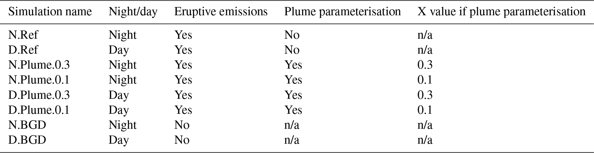
n/a: not applicable.

Regarding the composition of the volcanic emissions, we need to account for the modification of the volcanic emissions when magmatic gases first mix with ambient air at high temperature. The processes occurring at high temperature are not yet fully known and quantified as discussed in previous sections. Previous modelling studies showed that emissions of primary (or at source) volcanic sulfate aerosols and radicals such as Br, Cl or OH are necessary to kick-start the bromine explosion in the early stage of the plume (e.g. Roberts et al., 2009; Surl et al., 2021). The primary sulfate aerosols provide surface area to catalyse the bromine heterogeneous chemistry. The Br radicals provide an initial reactive halogen source that kick-starts the halogen chemistry. Br radicals may be produced both directly from high-temperature processes and indirectly from reactions involving HBr and high-temperature-produced HO_x. As in previous studies (e.g. Roberts et al., 2009; Jourdain et al., 2016; Surl et al., 2021) we take into account these changes from high-temperature processes in the volcanic emissions used in MOCAGE 1D simulations. The molar ratios and associated mass fluxes for the eruption introduced as input to the 1D MOCAGE model are given in Table 1. For H₂O, HCl, H₂S and CO, their molar ratio to SO₂ comes directly from the relative magmatic trace gas composition. For the emissions of primary sulfate aerosols, we use the ratios of SO₂ proposed by Surl et al. (2021) for their “main” model experiment simulating a case of Mount Etna passive degassing in 2012. For bromine, we use the $\mathrm{HBr}/{\mathrm{SO}}_{\mathrm{2}}$ ratio from Table 1 to get the total number of bromine moles that are then split into 75 % HBr and 25 % Br as in Surl et al. (2021). Note that because CO₂, HF and HI are not relevant for the bromine chemistry in volcanic plumes, they are not taken into account in this study. H₂ emission is not introduced since they are negligible with respect to background concentrations. H₂O emissions are not included because water vapour is considered as a meteorological variable in the troposphere in MOCAGE and set from the forcing meteorological model. In most previous modelling studies, H₂S and CO volcanic emissions have not been included. In Table 1, H₂S emissions are much smaller than SO₂ emissions. We checked a posteriori that H₂S and CO emissions are not important, making negligible changes in the model results with or without their inclusion.

The values given in Table 1 serve for the reference simulations called N.Ref for the eruption. To trigger fast initial production of BrO, Br emissions are included as in Surl et al. (2021). Surl et al. (2021) concluded that emitted OH's main effect on bromine chemistry was to produce Br radicals from HBr shortly after emission. In the absence of primary Br emissions, differing quantities of OH had an effect that had largely dissipated by 30 min after emission. Since our work aims at preparing 3D simulations at the regional and global scales at least over several hours and includes primary Br emissions, it is possible to neglect OH emission. Concerning NO_x that may also be produced by high temperatures, as explained before, it is not included in emissions in the reference simulations. However, additional experiments are done to test the sensitivity to the composition of the volcanic emissions, in particular including NO_x emissions, as detailed in Sect. 4.3.

The end time of the eruption (18:15 UTC) is very close to night-time. Thus, the role played by photochemistry in the plume can only be fully analysed when daylight comes back the day after (11 May in the morning with dawn daylight starting at 04:15 UTC). This is why we have also set another experiment called D.Ref that is the same as N.Ref except that the 4 h eruption occurs at the start of daytime from 04:15 UTC on 11 May instead of 14:15 UTC on 10 May, so that the bromine cycle is not stopped early by night-time conditions. The chemical initial conditions for these daytime simulations are from the same MOCAGE 3D simulation as for N.Ref but on 11 May at 04:00 UTC. The daytime simulations do not represent that particular eruption but are of interest for studying the bromine cycle in daylight conditions – conditions which are most favourable to the bromine cycle. These simulations are run until 11 May 18:00 UTC, just before night. Note that the simulations run with the eruption stopping at 18:15 UTC and including night-time conditions are referenced as “N.”, and those run over only daytime with the eruption stopping at 08:15 UTC are referenced as “D.”.

Another parameter that needs to be set in the simulations is the effective radius of the sulfate aerosols (R_eff) corresponding to the mean-surface-area-weighted radius. It is used to calculate the total surface of sulfate aerosols which is one of the parameters of the heterogeneous reaction rate constants (Reactions R5a, R5b and R6). A few studies give an estimate of the value of the sulfate aerosol radii within Mount Etna plumes close to the vent (Watson and Oppenheimer, 2000, 2001; Spinetti and Buongiorno, 2007; Roberts et al., 2018). Watson and Oppenheimer (2000, 2001) measured a mean effective radius of ∼ 0.7 to 0.85 µm in Mt Etna's plumes. Spinetti and Buongiorno (2007) airborne observations of Mt Etna's plumes gave R_eff = ∼ 1 µm. More recently, Roberts et al. (2018) found R_eff = 0.3 µm from measurements of aerosol size distributions gathered in passive emissions of Mt Etna. R_eff is expected to vary depending on the environmental conditions and the characteristics of the emission. The differences between these studies may also come from limitations of the aerosol observations used, in particular regarding the sampling of small particles that can be underestimated. This is why we choose here R_eff = 0.3 µm from Roberts et al. (2018) since this value was inferred from ash-free observations in quiescent degassing over a wide range of aerosol sizes, including small size particles.

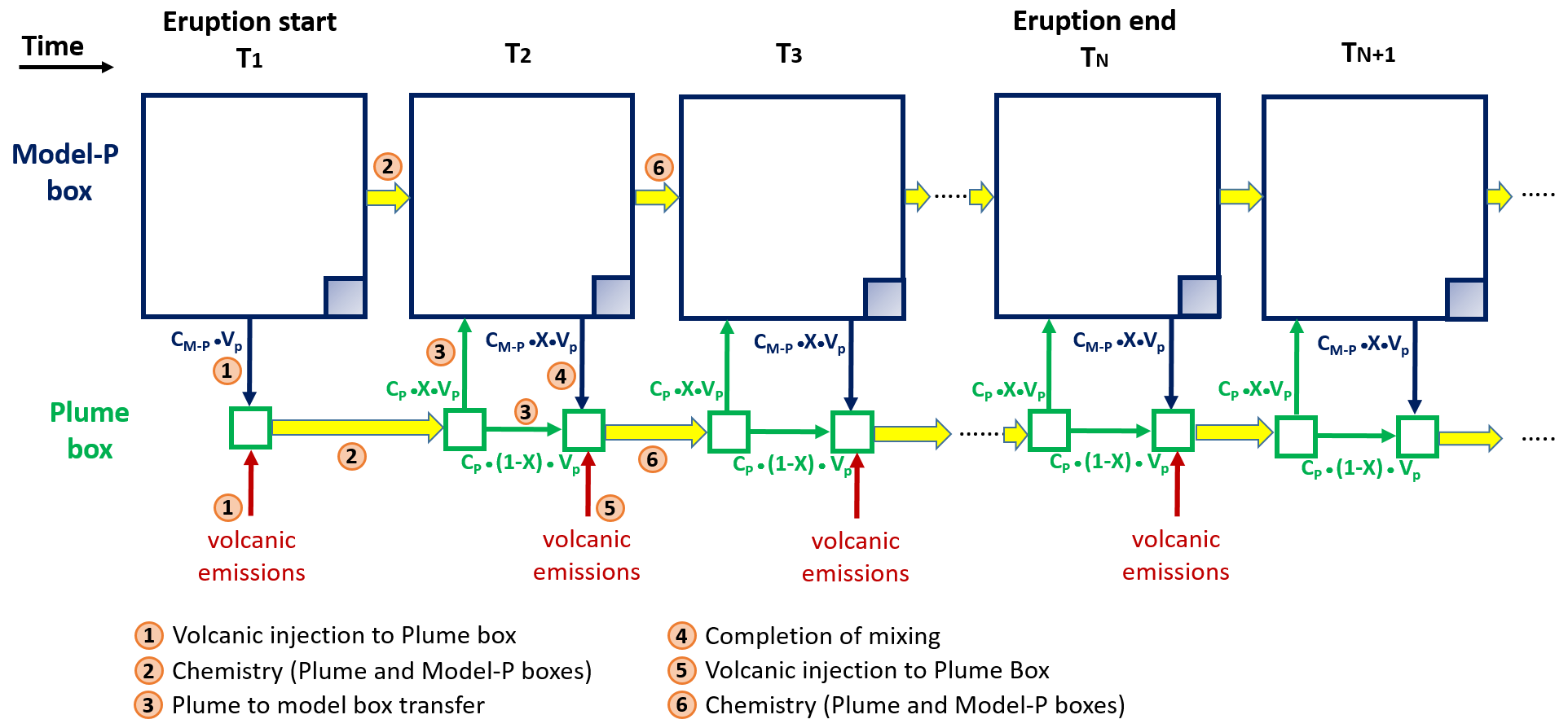
Figure 1 Schematic representation of the plume parameterisation. At the time step corresponding to the start of the eruption the plume box and the model-P box are defined: the plume box has a volume (V_P) of 0.025^∘ × 0.025^∘ × height and model-P box is defined as the model box (0.5^∘ × 0.5^∘ × height) minus V_P (big blue square minus the shaded blue square), whose volume is noted V_M-P. The concentrations in the plume box and model-P boxes are noted C_P and C_M-P, respectively. (Step 1) At T₁, the plume box initial chemical concentrations are the background concentrations from the model-P box plus the volcanic emissions over the time step (15 min). (Step 2) The chemistry is applied separately to the plume box and to the model-P box (big arrows in yellow colour). (Step 3) At T₂, a fraction X of the molecules contained in the plume box C_P ⋅ (X ⋅ V_P) are transferred to the model-P box and (1 − X) ⋅ V_P kept in the plume box. (Step 4) To complete the mixing between plume and model-P boxes, the model-P box transfers C_M-P ⋅ X ⋅ V_P to the plume box. It is at this step that the concentrations in the model box are output from adding model-P + plume concentrations. (Step 5) The concentration of the plume box is then updated by adding the volcanic emissions calculated from the emission flux (Table 1) over the 15 min model time step. (Step 6) The chemistry is applied separately to the plume box and to the model-P box (big arrows in yellow colour). For the subsequent model time steps until the end of the eruption, steps 3 to 6 are repeated. After the end of the eruption, steps 3, 4 and 6 are repeated, i.e. excluding the step of volcanic emissions.

The reference simulations are listed in Table 2. Additionally, the N.BGD (respectively D.BGD) simulation is run with no volcanic emissions in night-time (respectively daytime) conditions to characterise the background chemical conditions for appropriate species.

4.2 Plume parameterisation

The study is focused on a 1D model but using the characteristics of the 3D MOCAGE model. Three-dimensional chemical models resolve the chemical reactions at the grid box scale with the assumption that chemical species are homogeneously distributed within each grid box. However, within a volcanic plume, the bromine chemistry takes place within a smaller volume compared to the usual volume of MOCAGE grid boxes: from 2^∘ × 2^∘ to 0.5^∘ × 0.5^∘ for global simulations and from 0.5^∘ × 0.5^∘ to 0.1^∘ × 0.1^∘ for regional simulations. Thus, at the grid scale of global models, volcanic eruption plumes can be considered as a subgrid-scale phenomenon. Processes occurring at subgrid scales are typically represented via parameterisations in atmospheric models. For atmospheric plume modelling, the plume-in-grid approach is the most widely used (see review by Karamchandani et al., 2011), in particular for air quality applications, giving a better description of the phenomenon studied. The principle of the plume-in-grid approach is to use a reactive plume model in addition to the 3D model. This reactive plume model is a representation of three-dimensional puffs. We propose here a simple version of the plume-in-grid approach that is designed to evaluate the effect on the bromine explosion cycle of the assumption that chemical species are homogeneously distributed within each model grid box. The basis of what we call hereafter the plume parameterisation is to represent the subgrid-scale chemical reactions at the plume scale only in the model vertical column in which the volcano is located, as in Grellier et al. (2014). It consists of computing the chemical reactions defined by the model within a volume of 0.025^∘ × 0.025^∘ × height (∼ 2.5 km × ∼ 2.5 km × height) of the grid box (called hereafter plume box) representative of the plume area, which is much smaller than the model grid volume (called hereafter the model box). Therefore, the ratio of the volume of the plume box over the model box equals $\mathrm{1}/\mathrm{400}$. We also define the model-P box, which is the model box minus the volume of the plume box (volume model-P box/volume model box = 399/400). This plume parameterisation is composed of the following steps that are also illustrated in Fig. 1 with details given in the figure caption.

• Step 1. At the first time step when the eruption occurs, the plume box chemical concentrations are the sum of the concentrations from the model-P box (proportionally to the volume of the plume box) and of the volcanic emissions over the 15 min model time step.

• Step 2. The chemistry is applied in parallel to the plume box and to the model-P box.

• Step 3. At the beginning of the second time step, a fraction X of the molecules contained in the plume box are transferred to the model-P box, and the remaining part is kept in the plume box.

• Step 4. To complete the mixing between the plume and model-P boxes, the model-P box transfers its concentrations to the plume box proportionally to the volume of the plume box. It is at this step that the concentrations in the model box are output from adding model-P+plume concentrations.

• Step 5. The volcanic emissions are added to the concentration of the plume box.

• Step 6. The chemistry is applied in parallel to the plume box and to the model-P box.

For the next time steps until the end of the eruption, we repeat steps 3 to 6. After the end of the eruption, we assume that the dilution continues with the same X coefficient, meaning that we exclude the step of volcanic emissions (Step 5) and only do steps 3, 4 and 6. The X coefficient ranges between 0 and 1. A low (respectively high) value of X corresponds to a weak (respectively strong) dilution of the plume box with the model-P box at each time step (15 min).

Grellier et al. (2014) had proposed only two possibilities for the computation of the mixing. One was to add the full content of the plume box to the model-P box at each model time step (called plume 1) corresponding to X = 1. In this case, the content of the plume box undergoes complete mixing with the model-P box every 15 min. The second possibility was to add the plume box content to the model-P box only at the end of the eruption (called plume 2). In this case, the plume is isolated from the model grid box during the eruption (corresponding to X = 0) and then fully mixes with the model-P box at the time step of the end of the eruption. These two possibilities correspond to two extreme assumptions for the dilution of the plume, but neither of them is realistic. This is why we developed the intermediate and more realistic approach with a partial mixing during and after the eruption based on the coefficient X as explained above. Note that X = 1 is different from N.Ref. In the simulation N.Ref, the emissions are injected at each time step in the model box, meaning that they are directly diluted in the model box and react with the molecules of all species present in the model box. In the plume simulation with X = 1, the emissions are injected at each time step in the plume box, then the chemistry is applied to the plume box and finally the content of the plume box is fully mixed with the model-P box at each time step.

X represents the fraction of the molecules contained in the plume box of size ∼ 2.5 km × 2.5 km that are mixed with the model-P box a size of ∼ 50 km × 50 km. In reality, the mixing varies with the plume characteristics and the meteorological conditions. This is why we test two values of X here: X = 0.3 and X = 0.1. This corresponds to a mixing rate of 0.76 per hour for X = 0.3 and 0.34 per hour for X = 0.1, giving a sensible range for full dilution time of ∼ 2.5 h for X = 0.3 and ∼ 10 h for X = 0.1 after the end of the eruption.

Note that our method indirectly represents the transport of the plume within the model box by the fact that we simulate the progressive dilution of the plume with the background air of the model-P box. The plume box is only used to calculate the chemical processing of the emissions within an air volume typical of the size of a volcanic plume. Ultimately, we are interested in analysing the effect of this processing on the final partitioning of the bromine species at the scale of the model box.

The simulations including the subgrid-scale plume parameterisation are listed in Table 2.

4.3 Sensitivity tests

Several sensitivity tests were performed regarding the emission amount and composition and the primary sulfate characteristics. These simulations are only run in the daytime configuration in order to best follow the bromine explosion since the night configuration stops BrO production very rapidly just after the end of the eruption. Also because daytime simulations are shorter (14 h) and the maximum of BrO is reached not long after the end of the eruption (e.g. < 2 h in D.Ref simulation), there is less of an expected effect arising from the assumption of no exchange between the selected 1D column and its surrounding background air. These sensitivity simulations are performed with the subgrid-scale parameterisation only when relevant.

Table 3 Characteristics of the test simulations on the amount of emissions and on the total $\mathrm{bromine}/{\mathrm{SO}}_{\mathrm{2}}$ ratio.

n/a: not applicable.

Roberts et al. (2014) and Roberts (2018) showed that the relative production of BrO from HBr depends on the emission flux and on the total bromine $(\mathrm{HBr}+\mathrm{Br})/{\mathrm{SO}}_{\mathrm{2}}$ ratio of the emissions. This is why sensitivity simulations are run with lower emission fluxes for all species and with a lower total $\mathrm{bromine}/{\mathrm{SO}}_{\mathrm{2}}$ ratio including also the subgrid-scale parameterisation since the bromine partition may depend in these cases on the size of the box considered and associated concentrations. Their characteristics are given in Table 3.

Table 4 Characteristics of the other test simulations described in Sect. 4.3. For the primary sulfate aerosols, the percentage corresponds to the ratio to SO₂.

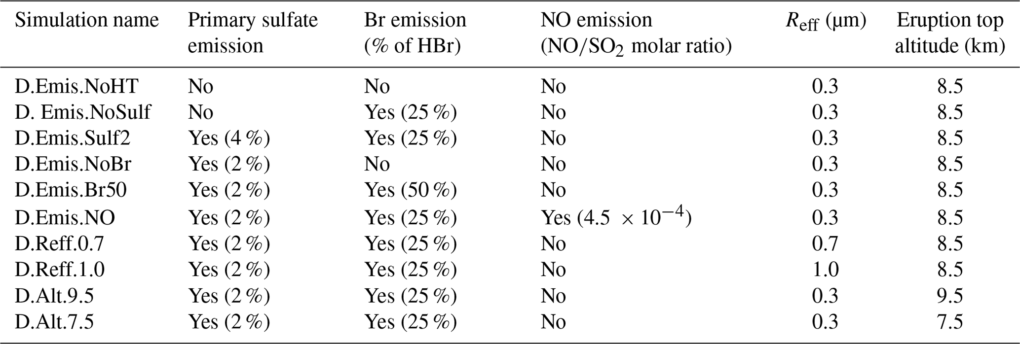
Other sensitivity simulations are listed in Table 4. Firstly, we analyse the sensitivity of the rapid formation of BrO to the composition of the volcanic emissions, in particular to assess the individual impact of the additional species produced at the vent and by high-temperature processes (Br and primary sulfate). We also run simulations with different $\mathrm{Br}/\mathrm{HBr}$ and primary $\mathrm{sulfate}/{\mathrm{SO}}_{\mathrm{2}}$ ratios since these ratios vary naturally with the characteristics of the volcano's emissions and their environmental conditions and also because their determination is still uncertain as discussed in previous sections. In addition to Br emissions, we also test the inclusion of oxidants in the form of NO_x that are possibly formed at high temperatures. For this, we use the $\mathrm{NO}/{\mathrm{SO}}_{\mathrm{2}}$ molar ratio of 4.5 × 10⁻⁴ of Surl et al. (2021).

Another important parameter that drives the bromine explosion is the total surface area of sulfate aerosols for the heterogeneous reactions. It is calculated in our simulations from the sulfate concentration and the R_eff parameter. Because of the natural variations of R_eff and the uncertainties on its estimation from observations, we performed sensitivity tests with other R_eff values based on estimates of R_eff from previous studies (see Sect. 4.1): R_eff = 0.7 µm and R_eff = 1.0 µm instead of R_eff = 0.3 µm in the reference simulations. Apart from R_eff, their settings are the same as in the D.Ref simulation. Thus, for a given sulfate concentration, a higher R_eff leads to a fewer number of larger particles and a lower aerosol surface area.

Among the parameters that may not be well observed, there is also the top altitude of the eruption. For volcanoes located in remote places, this altitude can be estimated from satellite observations but with uncertainties (e.g. Scollo et al., 2014; Corradini et al., 2020). This is why we test here the influence of the top height of the eruption, ranging from 7.5 to 9.5 km.

5 Results

All the results shown in this section are partial column concentrations vertically integrated over the volcanic emission levels in molecules per square centimetre ($\mathrm{molec}.{\mathrm{cm}}^{-\mathrm{2}}$), i.e. from 3300 to 8500 m in all simulations except for the sensitivity simulations to the top altitude of the eruption for which the top altitude is 7500 or 9500 m instead of 8500 m. The figures show the concentrations in the model box. For the Plume.0.3 and Plume.0.1 simulations, the concentrations in the model box come from adding the model-P box and the plume box concentrations at each 15 min time step. Note that because the eruption starts at 14:15 UTC for N. simulations (respectively 04:15 UTC for D. simulations) and the main time step of the model is 15 min, the effect of the emissions is only visible in the figures at 14:30 UTC (respectively 04:30 UTC for D. simulations).

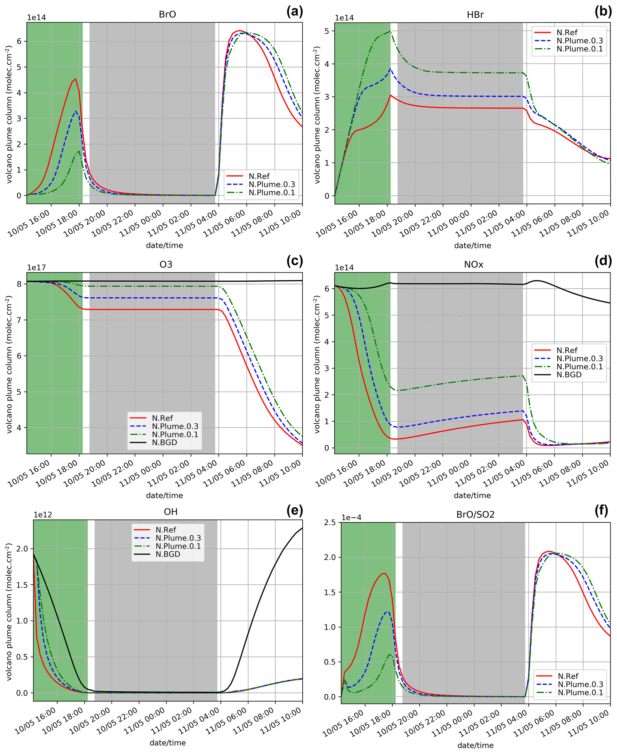
Figure 2 Time evolution from 14:15 UTC of the column number of molecules of BrO (a), HBr (b), O₃ (c), NO_x (d), and OH (e) by unit surface and of the ratio $\mathrm{BrO}/{\mathrm{SO}}_{\mathrm{2}}$ (f) within the model box (model-P box + plume box) for the N.Ref, N.Plume.0.3, and N.Plume.0.1 and N.BGD where appropriate. The quantities are integrated vertically on the emission levels (3300–8500 m). The green zone corresponds to the 4 h of the volcanic eruption emission (14:15–18:15 UTC) and the light grey zone to night-time.

5.1 Analysis of the reference and plume parameterisation simulations for the eruption starting in the afternoon

The time evolution of the column of BrO, HBr, O₃, NO_x, OH and the ratio $\mathrm{BrO}/{\mathrm{SO}}_{\mathrm{2}}$ (in red) for the N.Ref simulation is shown in Fig. 2. Additionally, the partitioning between the bromine species for N.Ref is shown in Fig. 3a. BrO (Fig. 2a) formation is triggered just after the start of the eruption and increases rapidly until 17:45 UTC. During this period, HBr is efficiently converted into BrO (up to 55 %) and a small part into HOBr (5 %) (Fig. 3a). The Br contribution to the total bromine is very low because of its very rapid conversion to BrO. BrONO₂ has only a small contribution to the total bromine because it is efficiently depleted by hydrolysis. After 17:45 UTC and before the full night, the daylight starts to decrease significantly, and this strongly reduces the efficiency of the bromine explosion even if there are still bromine emissions. This is linked to a weakening of the photolysis of Br₂ and BrCl. This is also why Br₂ and to a lesser extent BrCl increase during those time steps (see Fig. 3a).

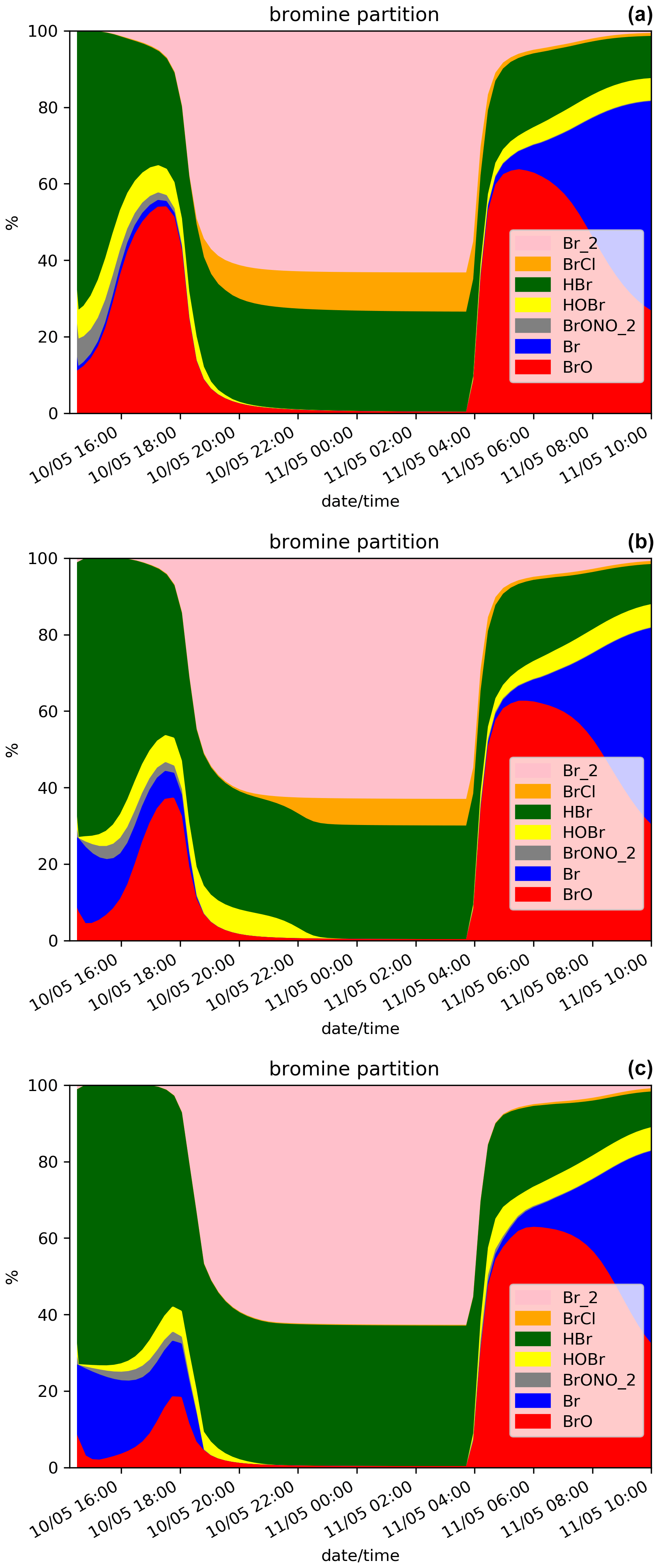
Figure 3 Time evolution from 14:15 UTC of the relative partition of the bromine species in percent (%) for N.Ref and (a), for N.Plume.0.3 (b) and for N.Plume.0.1 (c) simulations within the model box. The partition is calculated from total bromine Br_y with Br_y = $\mathrm{HBr}+\mathrm{BrO}+\mathrm{Br}+\mathrm{2}{\mathrm{Br}}_{\mathrm{2}}+\mathrm{BrCl}+\mathrm{HOBr}+{\mathrm{BrONO}}_{\mathrm{2}}$.

At night-time BrO disappears after about 1 h to produce reservoir species, mainly Br₂ and to a lesser extent BrCl. Br₂ production is dominant (Reaction R5a) with respect to BrCl (Reaction R5b) at high $\mathrm{HBr}/\mathrm{HCl}$ ratio. But because HBr is largely depleted before night, the $\mathrm{HBr}/\mathrm{HCl}$ ratio becomes small enough to lead to some production of BrCl. The fraction of HBr remaining from the emission and not converted into BrO before sunset is stable during the night because of the lack of photolysis.

On the day after the eruption (11 May) upon sunrise, the bromine cycle starts again, using HBr to produce BrO rapidly until ∼ 05:30 UTC (max ∼ 6.5 × 10¹⁴ $\mathrm{molec}.{\mathrm{cm}}^{-\mathrm{2}}$). After ∼ 05:30 UTC, the contribution of Br increases while BrO decreases (Fig. 3) because of decreasing concentrations of O₃ (Fig. 2d). Such an increase in Br was also found in the model results at the regional scale of Jourdain et al. (2016) from 70 km downwind from the Ambrym vent. Here the Br enhancement is expected to be stronger than in Jourdain et al. (2016) towards the end of the simulation since we assume no mixing with air outside the 1D column leading to a lack of oxidants that could come from background surrounding air. Figure 2c shows that the halogen (chlorine and bromine) cycling, including the production of BrO, depletes ozone significantly in the plume during daytime on the day of the eruption and even further on the day after, leading to about half of the initial ozone at the end of the N.Ref simulation.

During daytime on the day of the eruption and on the day after, the bromine cycle leads to an O₃ decrease (Fig. 2c) together with NO_x (Fig. 2d), OH (Fig. 2e) depletion and HNO₃ formation (not shown). Overall, the results of the N.Ref simulation (bromine partition and depletion of oxidants) are consistent with previous modelling studies of bromine in volcanic plumes (e.g. Roberts et al., 2009; Jourdain et al., 2016; Surl et al., 2021).

To characterise the efficiency of the bromine cycle in the plume compared to observations, we calculate the $\mathrm{BrO}/{\mathrm{SO}}_{\mathrm{2}}$ ratio. The simulated values of $\mathrm{BrO}/{\mathrm{SO}}_{\mathrm{2}}$ are well within the range of variation of the observed $\mathrm{BrO}/{\mathrm{SO}}_{\mathrm{2}}$ ratio at Mt Etna (Gutmann et al., 2018). In the simulation, the time variation of the $\mathrm{BrO}/{\mathrm{SO}}_{\mathrm{2}}$ ratio (Fig. 2f) is similar to BrO (Fig. 2a). Note that at 14:30 UTC, the first time step when the emissions are injected and have been processed chemically, $\mathrm{BrO}/{\mathrm{SO}}_{\mathrm{2}}$ shows a stronger gradient compared to the next time steps. This is because the 14:30 UTC time step benefits from high background OH concentrations that are largely used to produce BrO from Reactions (R1) and (R2), in addition to the production of BrO through heterogeneous reactions. At later time steps, there is less OH leading to less steep variations of BrO.

In addition to the comparison with the literature (Gutmann et al., 2018), we analyse if the simulation gives reasonable estimates by comparing BrO and SO₂ integrated columns to satellite retrievals from the GOME-2 space-borne instrument (supplement of Hörmann et al., 2013) in the Mt Etna plume on 11 May at 08:40 UTC, originating from the 10 May eruption. For GOME-2, the data correspond to slant column densities and are therefore slightly different from the model-derived columns. Note that the model results are the partial columns over the emission levels, but they can be assimilated to tropospheric columns since background SO₂ concentrations are by far lower than those from the eruption and bromine species are initialised to zero in the troposphere. The GOME-2 BrO and SO₂ maxima are 2.3 × 10¹⁴ and 1.6 × 10¹⁸ $\mathrm{molec}.{\mathrm{cm}}^{-\mathrm{2}}$, respectively. The N.Ref simulation at the time of GOME-2 observations gives BrO and SO₂ columns of 3.5 × 10¹⁴ and 3.1 × 10¹⁸ $\mathrm{molec}.{\mathrm{cm}}^{-\mathrm{2}}$, respectively. The observed and simulated values of BrO and SO₂ are reasonably close, although higher in the simulations. There are several explanations for this. The absence of transport and deposition in the 1D MOCAGE simulations leads to no dilution of the plume or loss by deposition and thus to an expected overestimation compared to observations. Moreover, the concentrations of the chemical species are representative of a larger surface area in the observations compared to the model, with the satellite pixel being 40 km × 80 km and the model grid box being ∼ 44 km × ∼ 55 km. Overall, the agreement is very good, considering also the uncertainties of the satellite estimates of SO₂ and BrO columns and of the estimates of the volcanic gas fluxes and their composition used in MOCAGE. An additional and pertinent way to evaluate the simulation is to compare $\mathrm{BrO}/{\mathrm{SO}}_{\mathrm{2}}$ ratios. The N.Ref $\mathrm{BrO}/{\mathrm{SO}}_{\mathrm{2}}$ ratio (1.13 × 10⁻⁴) is consistent with the ratio of integrated molecules within the plume from GOME-2 (1.24 ± 0.19) × 10⁻⁴ (Hörmann et al., 2013), showing a realistic production of BrO in the model.

Figure 2 also shows the time evolution of the species for N.Plume.0.3 and N.Plume.0.1 simulations – simulations using the plume parameterisation. The partition of the bromine species for N.Plume.0.3 and N.Plume.0.1 is depicted in Fig. 3. N.Plume.0.3 and N.Plume.0.1 have similar overall variations to N.Ref. However, during the eruption, when applying the plume parameterisation, BrO maximum values (Fig. 2a) are lower and correspond to higher values of HBr (Fig. 2b) and ozone (Fig. 2c). This is due to the number of molecules of oxidants (O₃, HO_x, NO_x) available in the plume box that is lower than in the model box because of the volume difference. This limits the bromine explosion cycle in the plume box and therefore BrO production. This is consistent with the bromine partitioning shown in Fig. 3 that with less dilution between the plume box and the model-P box (from X = 0.3 in N.Plume.0.3 to X = 0.1 in N.Plume.0.1), less Br is converted into BrO. Ozone (Fig.2c), NO_x (Fig. 2d) and OH (Fig. 2e) depletion occurs during the eruption thanks to BrO net formation, but this gets less strong in the model-P box as the dilution decreases (lower X coefficient). The time variation of the $\mathrm{BrO}/{\mathrm{SO}}_{\mathrm{2}}$ ratio (Fig. 2f) is consistent with that of BrO (Fig. 2a). The main difference is visible from the first time steps of the volcanic emission. At 14:30 UTC when the emission is first taken into account, there is an increase in $\mathrm{BrO}/{\mathrm{SO}}_{\mathrm{2}}$ in N.Plume.0.3 and N.Plume.0.1 because the plume box was initialised with background concentrations providing enough oxidants to produce BrO. In the time step after (14:45 UTC), there are less oxidants available in the plume box and yet not very much of the emissions transferred to the model-P box to produce BrO efficiently in the model-P box. From 15:00 UTC, $\mathrm{BrO}/{\mathrm{SO}}_{\mathrm{2}}$ increases mainly because of BrO production in the model-P box from the partial mixing with the emission-rich plume box at each time step. With low X, this mixing is slow, leading to a less steep $\mathrm{BrO}/{\mathrm{SO}}_{\mathrm{2}}$ ratio increase. This behaviour of the plume parameterisation is consistent with the observed and modelling results within the core volcanic plumes (e.g. Bobrowski et al., 2007; Jourdain et al., 2016; Rüdiger et al., 2021) where mixing controls the production of BrO by limiting the availability of oxidants. Such studies show that BrO production is limited by the amount of oxidants available and that BrO production is higher at the edge of plumes where there is mixing with oxidant-rich background air compared to within the plume core. Note that this effect depends on volcanic conditions (Roberts et al., 2018). It was checked that the $\mathrm{BrO}/{\mathrm{SO}}_{\mathrm{2}}$ decrease from 14:45 to 15:15 UTC is actually due to the oxidant-limited chemistry in the plume and not related to the 15 min time step by running simulations with a 1 min time step.

At night, the partition of the bromine species is different in the three simulations (Fig. 3). In N.Plume.0.1, the reservoir species at night is Br₂ only since the $\mathrm{HBr}/\mathrm{HCl}$ ratio is such that Reaction (R5b) is not active. N.Plume.0.3 simulations show an intermediate situation which favours firstly Br₂ production until the $\mathrm{HBr}/\mathrm{HCl}$ ratio is sufficient to trigger the production of BrCl via Reaction (R5b). As in N.Ref, Br₂ and BrCl concentrations are stable in time once HOBr is fully depleted.

In the daytime on 11 May (from 04:15 UTC), the maxima of BrO and the $\mathrm{BrO}/{\mathrm{SO}}_{\mathrm{2}}$ ratio in N.Plume.0.3 and N.Plume.0.1 simulations reach values close to the N.Ref simulation but are slightly lower and occur a bit later as X (dilution coefficient) decreases from 0.3 to 0.1. The BrO and HBr concentrations tend to converge for all simulations on 11 May from 05:00 UTC consistently with the partitioning between the bromine species that is very similar in the three simulations (Fig. 3). This is because the day after the eruption the emissions injected in the plume box had enough time to be fully diluted in the model-P box. O₃ strongly decreases from 11 May 04:15 UTC in N.Plume.0.3 and N.Plume.0.1 as in N.Ref with small differences for N.Plume.0.1 at the end of the simulation linked to a slightly lower net production of BrO. As for N.Ref, results from the plume parameterisation simulations for the $\mathrm{BrO}/{\mathrm{SO}}_{\mathrm{2}}$ ratio at the time of the observations are within the GOME-2 estimated range ((1.24 + 0.19) × 10⁻⁴) with 1.15 × 10⁻⁴ and 1.17 × 10⁻⁴ for N.Plume.0.3 and N.Plume.0.1, respectively. These modelled values are consistent with the typical values of $\mathrm{BrO}/{\mathrm{SO}}_{\mathrm{2}}$ measured in Mt Etna's plumes (Gutmann et al., 2018). Note also that they are not very different from N.Ref because of a similar behaviour of the plume simulations the day after the eruption.

In summary, the MOCAGE 1D simulations provide results consistent with observations and with previous modelling studies. This means that the MOCAGE 1D model, with the update to the MOCAGE chemical scheme to account for the halogen plume chemistry, is able to simulate well the bromine cycle in volcanic plumes. The use of the plume parameterisation changes the results mainly during the eruption by reducing BrO net production similarly to what occurs in the core of the plume because of less oxidants being available. The results of the simulations with and without the plume parameterisation converge on the day after the eruption because most of the plume emissions are already diluted in the model grid box giving a similar efficiency of HBr conversion to reactive bromine. The effect of the parameterisation is only to slightly reduce and delay the $\mathrm{BrO}/{\mathrm{SO}}_{\mathrm{2}}$ maximum.

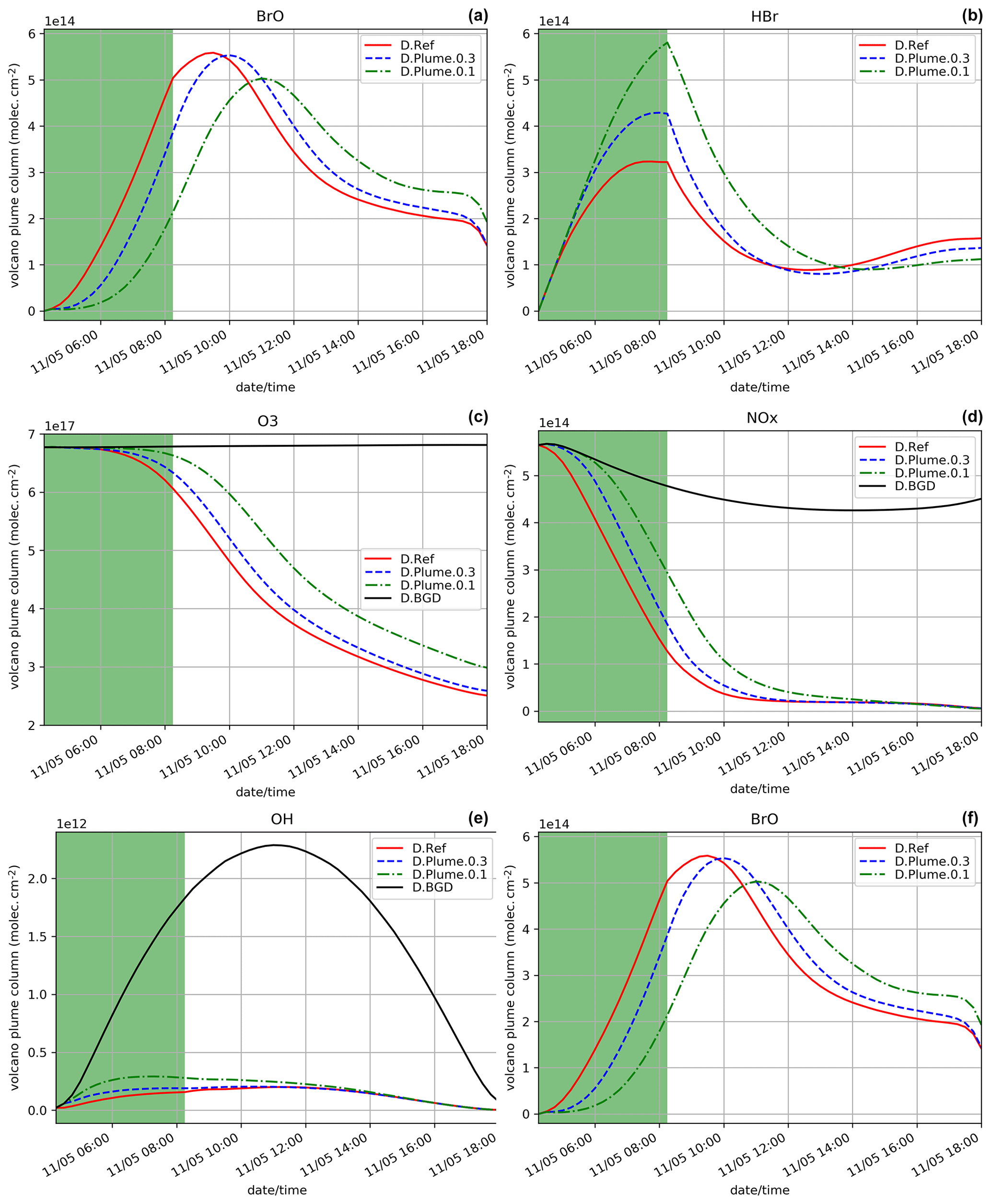
Figure 4 Similar to Fig. 2 but for the daytime simulations D.Ref, D.Plume.0.3 and D.Plume.0.1 from 04:15 UTC. The green zone corresponds to the 4 h of the volcanic eruption emission (04:15–08:15 UTC).

5.2 Analysis of the reference and plume parameterisation simulations for the eruption starting early morning

Since the night starts just after the end of the eruption and photolysis plays a role in the bromine cycle, we also study the impact of the subgrid-scale parameterisation assuming an identical eruption emission but that takes place during daytime, from 04:15 UTC on 11 May instead of 14:15 UTC on 10 May. The results for D.Ref, D.Plume.0.3 and D.Plume.0.1 are displayed in Figs. 4 and 5. In Fig. 4, the D.Ref simulation shows a rapid increase in BrO and $\mathrm{BrO}/{\mathrm{SO}}_{\mathrm{2}}$ with time from HBr emissions, leading to strong decreases in ozone (Fig. 4c), NO_x (Fig. 4d) and OH (Fig. 4e) compared to background (D.BGD). BrO reaches a maximum of 5.7 × 10¹⁴ $\mathrm{molec}.{\mathrm{cm}}^{-\mathrm{2}}$ at ∼ 09:00 UTC, which is a bit lower than in N.Ref (eruption at the end of the day) on the day after the eruption (6.3 × 10¹⁴ $\mathrm{molec}.{\mathrm{cm}}^{-\mathrm{2}}$). This is explained by higher initial ozone concentrations on 10 May at 14:15 UTC.

When applying the plume parameterisation, the BrO maximum tends to be lower and to occur later with decreasing dilution coefficient. For X = 0.3 (D.Plume.0.3), at the time when BrO is at a maximum, ∼ 95 % of the plume box is already mixed with the model box. This is why the results of D.Ref and D.Plume.0.3 are similar with a maximum of ∼ 55 % of BrO in the partitioning of bromine species (Fig. 5a and b). For X = 0.1, the maximum is lower (∼ 5.0 × 0¹⁴ $\mathrm{molec}.{\mathrm{cm}}^{-\mathrm{2}}$) and occurs at 11:00 UTC, corresponding to ∼ 48 % of the bromine species (Fig. 5c). The lower dilution slows down the production of BrO since less molecules of oxidant species are available in the plume box compared to the model-P box. This leads to more HBr and more ozone remaining in the model box (model-P box + plume box) in the D.Plume.0.1 simulation. The differences between the plume simulations are higher in the D. than in the N. simulations. On the day after the eruption, BrO production in N. simulations is quicker because part of the HBr is transformed into the form of Br₂ and BrCl, which are rapidly photolysed and converted to BrO thanks to higher ozone and because the full mixing between plume and model-P box is already mostly reached, even in N.Plume.0.1. Note that at the very end of the D. simulation the rapid decrease in BrO is due to nightfall. The $\mathrm{BrO}/{\mathrm{SO}}_{\mathrm{2}}$ ratio (Fig. 4f) follows mostly BrO variations except for the first time steps of the emissions with the same behaviour as discussed for the N. simulations (Sect. 5.1).

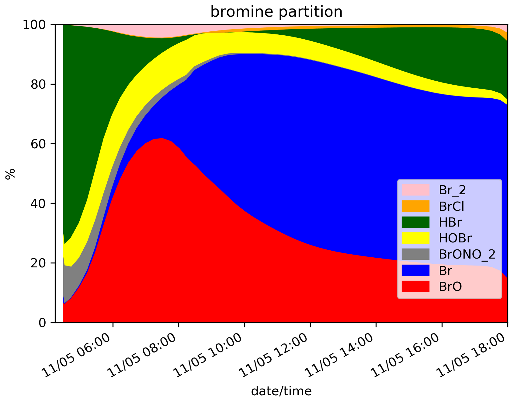
The bromine partitioning (Fig. 5) shows similarities between the D.Ref, D.Plume.0.3 and Plume.0.1 simulations. However, before the BrO maximum is reached, as the dilution coefficient decreases, there is more Br and less BrO. This behaviour is consistent with the results of the N. simulations (Fig. 3) before night-time. This is explained by ozone being quickly depleted in the plume box, slowing down the overall BrO production in the model box (model-P box+plume box). After the maximum of BrO is reached, Br increases while BrO decreases. Similarly to the N. simulations, this is due to decreasing concentrations of O₃.

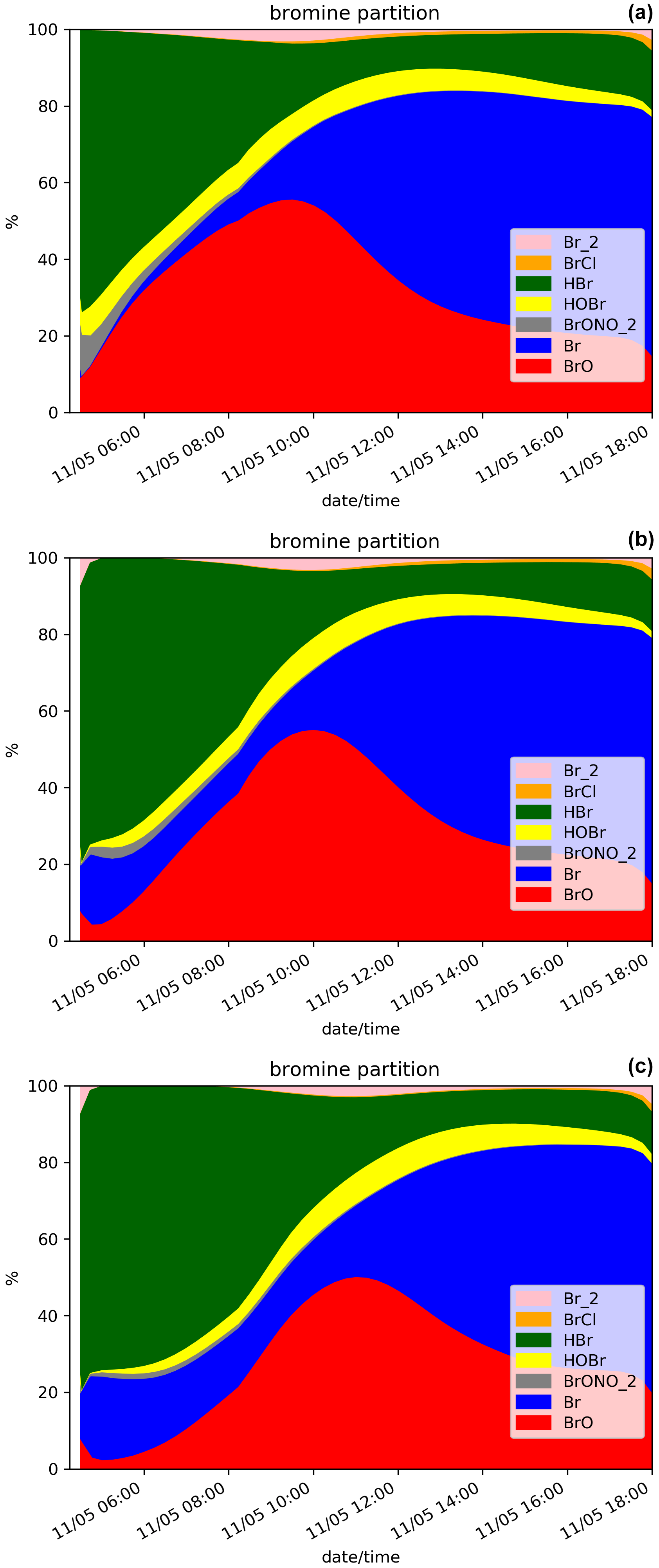
Figure 5 Similar to Fig. 3 but for the daytime simulations D.Ref (a), D.Plume.0.3 (b) and D.Plume.0.1 (c) from 04:15 UTC.

In summary, MOCAGE 1D early morning eruption experiments simulate the bromine cycle in a consistent way, and for D.Ref a maximum in BrO is reached about 1.5 h after the end of the eruption. As for the N. simulations, the plume parameterisation slightly delays BrO formation, and the maximum BrO reached is lower as the dilution coefficient decreases. There is an overall good consistency between the N. and D. simulations with differences due to the night interrupting BrO formation, higher initial ozone levels and more dilution of the plume in the model box at the time of the BrO maximum because it occurs later in the N. simulations.

5.3 Other sensitivity tests

Hereafter, we only discuss the sensitivity simulations starting on 11 May 04:00 UTC. Such D. simulations are consistent with N. simulations, but the bromine cycle is not interrupted by night. This leads to a shorter time to reach the BrO maximum in the D. configuration, meaning that there is less impact of the 1D-framework limitation linked to the assumption of no mixing with air surrounding the 1D model profile. It was checked that the results of the sensitivity simulations in N. configuration are consistent with those in D. configuration. The characteristics of the sensitivity tests discussed in this section are given in Tables 3 and 4. For the simulations not including the plume parameterisation (Table 4), it was checked that running MOCAGE 1D with both the plume parameterisation and the sensitivity parameters does not change the conclusions of the sensitivity analysis.

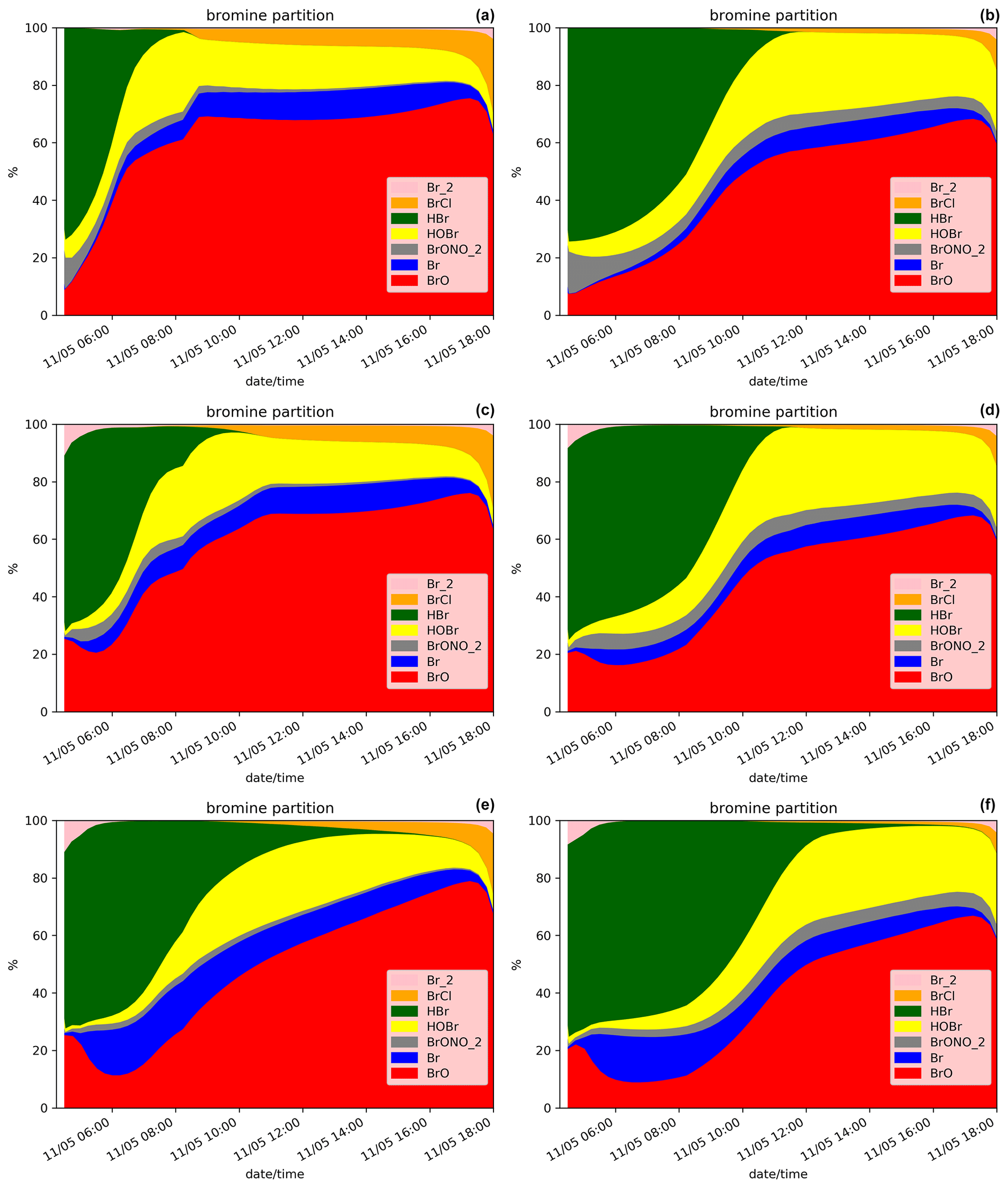
Figure 6 Similar to Fig. 5 but for the simulations D.LowHBr (a), D.Low.Emis (b), D.LowHBr.Plume.0.3 (c), D.LowEmis.Plume.0.3 (d), D.LowHBr.Plume.0.1 (e) and D.Low.Emis.Plume.0.1 (e).

5.3.1 Sensitivity to the total $\mathrm{bromine}/{\mathrm{SO}}_{\mathrm{2}}$ emission ratio and to the emission flux

The bromine partitioning from the simulations with a lower total $\mathrm{bromine}/{\mathrm{SO}}_{\mathrm{2}}$ emission ratio or a lower emission flux (Table 3) is shown in Fig. 6, including also the plume parameterisations (simulations D.LowHBr, D.LowHBr.Plume.0.3, D.LowHBr.Plume.0.1, D.LowEmis.Plume0.3 and D.LowEmis.Plume0.1).

Bromine partitioning in these simulations differs from the reference simulation D.Ref (Fig. 5). There is a much stronger decrease in HBr compared to D.Ref, and consequently there is more formation of BrCl (Reactions 5a and 5b). There is a stronger and more sustained increase in BrO, whilst the proportion of Br is lower than in D.Ref. Another difference lies in HOBr (and BrONO₂) which is proportionally higher in D.LowHBr and D.LowEmis than in D.Ref. These differences are related to the degree of mixing of oxidants relative to halogens in the plume (i.e. with relatively more oxidants for an emission with lower total $\mathrm{bromine}/{\mathrm{SO}}_{\mathrm{2}}$ or lower emission flux). The results are consistent with the 1D model sensitivity studies on gas flux and plume–air mixing of Roberts et al. (2014), although the time evolution of bromine speciation for this strong eruptive emission differs to the passive degassing case. The impact of the plume parameterisation when the total $\mathrm{bromine}/{\mathrm{SO}}_{\mathrm{2}}$ emission ratio is low (D.LowHBr.Plume.0.3, D.LowHBr.Plume.0.1, D.LowEmis.Plume0.3 and D.LowEmis.Plume0.1) is to cause an initial enhancement in the proportion of BrO in the first time steps of the eruption compared to D.LowHBr, while this effect was not seen in D.Plume.0.3 and D.Plume.0.1 compared to D.Ref. In the case of a low total $\mathrm{bromine}/{\mathrm{SO}}_{\mathrm{2}}$ ratio or emission flux, the composition in the plume box is such that there are sufficient oxidants (ozone, NO_x, HO_x) to produce BrO efficiently from HBr compared to D.Plume.0.3 and D.Plume.0.1. However, during these first time steps, these oxidants are rapidly consumed in the plume parameterisation cases, leading thereafter to a decrease in BrO with respect to HBr, which is more evident in D.LowHBr.Plume.0.1 and D.LowEmis.Plume0.1 because of its lower dilution coefficient. Over the duration of the simulation after the eruption injection, the higher oxidant-to-halogen ratio in these simulations compared to the reference leads to enhanced HOBr (formed from reaction of BrO with HO₂) and lower Br (removed by reaction of Br with O₃ to form BrO). There are some subtle differences between the simulations with lower emission flux (D.LowEmis, D.LowEmis.Plume.0.3 and D.LowEmis.Plume.0.1) and lower total $\mathrm{bromine}/{\mathrm{SO}}_{\mathrm{2}}$ emission ratio (D.LowHBr, D.LowHBr.Plume.0.3 and D.LowHBr.Plume.0.1): in the case of lower emission flux, the decrease in HBr is somewhat slower, and the proportion of HOBr is greater. This can be understood in terms of less aerosol surface available for heterogeneous chemistry in the lower emission flux case, resulting in slower conversion of HBr into reactive halogens and a smaller sink for HOBr. Overall, this sensitivity study emphasises the complex interplay between halogens, oxidants, and aerosol in the formation and partitioning of reactive halogen species including BrO through chemical reactions that in turn deplete the atmospheric oxidants.

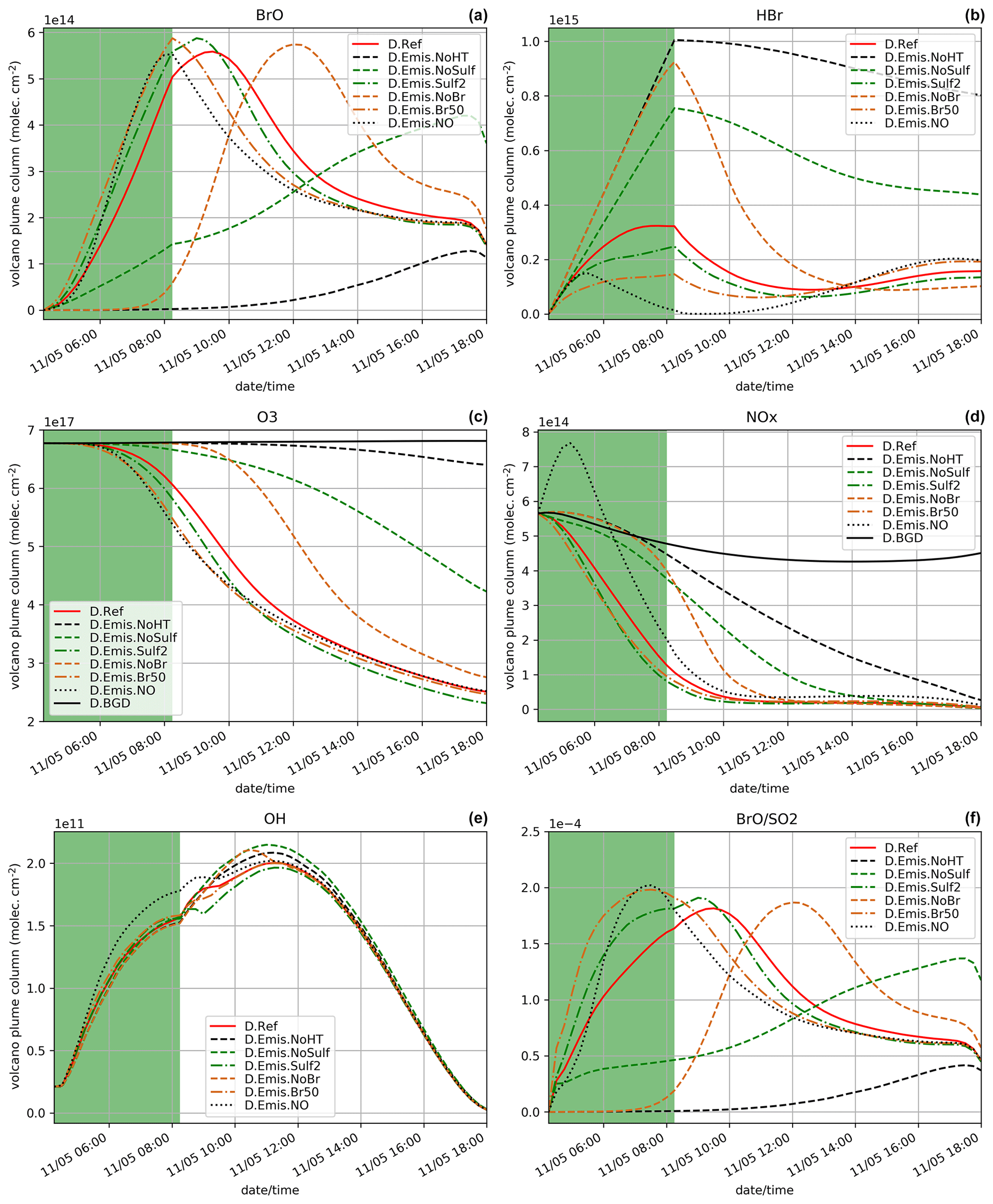
Figure 7 Similar to Fig. 4 but for the simulations testing the sensitivity to emission composition (in particular the primary sulfate and high-temperature products): D.Ref, D.Emis.NoHT, D.Emis.NoSulf, D.Emis.Sulf, D.Emis.NoBr, D.Emis.Br50, D.Emis.NO and D.BGD when appropriate. Details on these simulations are given in Table 4.

5.3.2 Sensitivity to the emission composition from high-temperature processes

We analyse here the sensitivity of the bromine cycle to variations in the composition of the emissions resulting from high-temperature processes (see Table 4). The results of these tests are depicted in Fig. 7.

D.Emis.NoHT simulation corresponds to the use of the raw magmatic gas emissions from Table 1, meaning not accounting for the change of composition at high temperature when magmatic gases first encounter atmospheric air. We know that this simulation is not realistic but it gives the lower bound of BrO production since it corresponds to emissions without Br radicals and primary sulfate. D.Emis.NoHT simulations show very slow production of BrO (Fig. 7a) from HBr (Fig. 7b) with a maximum of BrO ∼ 1.2 × 10¹⁴ (Fig. 7a). This is consistent with previous modelling studies (e.g. Roberts et al., 2009) showing the crucial role of species formed at vent to kick-start the bromine cycle. In the D.Emis.NoHT simulation, the bromine cycle is not complete before night and HBr, O₃ (Fig. 7c) and NO_x (Fig. 7d) depletion is weak.

D.Emis.NoSulf and D.Emis.Sulf2 are used to analyse the importance of primary sulfate. Without sulfate in the emissions (D.Emis.NoSulf), the bromine cycle is more efficient than in D.Emis.NoHT but is still much slower than in D.Ref. BrO is still increasing just before night with a maximum of only ∼ 4.2 × 10¹⁴, indicating that BrO net production is likely not completed during daytime. In D.Emis.NoSulf, the sulfate aerosols required for the heterogeneous reactions are only formed from volcanic SO₂ emissions through its reaction with OH (secondary sulfate). This process takes time and thus slows down BrO increase. Still this shows that these secondary sulfate aerosols from SO₂ emissions play a significant role when the plume is ageing. When primary sulfate emissions are doubled (D.Emis.Sulf2), there is a slight increase in BrO maximum reached about 0.5 h earlier compared to D.Ref. Higher primary sulfate concentrations enhance heterogeneous reactions and thereby speed up the production of BrO from HBr (Fig. 7b) and the depletion of ozone (Fig. 7c) and NO_x (Fig. 7d). However, the differences between D.Ref and D.Emis.Sulf2 are not very large, showing that the primary $\mathrm{sulfate}/{\mathrm{SO}}_{\mathrm{2}}$ ratio chosen in D.Ref is sufficient to provide a rapid bromine explosion. Note that the sulfate from background air was not accounted for in the initial conditions of our simulations in order to only analyse the effect of the volcanic emissions. If background sulfate is used in the simulations, it adds to the primary sulfate and therefore can increase BrO net production from heterogeneous reactions. In this study aerosol is dominated by the primary sulfate emissions, but background and secondary sulfate likely play an important role in the halogen chemistry of dispersed volcanic plumes and should be considered in future 3D regional and global simulations.

D.Emis.NoBr and D.Emis.Br50 simulations test the sensitivity to the emission of Br radicals produced from high-temperature processes. If no Br emission is assumed (D.Emis.NoBr), the production of BrO follows a curve similar to D.Ref but with a shift of ∼ 2.75 h later (Fig. 7a). When the partitioning of $\mathrm{Br}/\mathrm{HBr}$ in the emission is assumed to be $\mathrm{50}/\mathrm{50}$ (D.Emis.Br50) instead of $\mathrm{25}/\mathrm{75}$ (D.Ref), the $\mathrm{BrO}/{\mathrm{SO}}_{\mathrm{2}}$ maximum is slightly higher and occurs just at the end of the eruption, 1.25 h earlier than in D.Ref. Half of HBr is already in Br form in the D.Emis.Br50 simulation, and the BrO production rate is as expected increased in this simulation. Note that this maximum is as high as in the D.Emis.Sulf2 simulation, showing that both primary sulfate and Br emissions can be as important to rapid BrO formation. However, because Br concentration has a direct effect on BrO production while sulfate has an indirect effect through heterogeneous reactions, the maximum in D.Emis.Br50 is reached about 1 h earlier than in D.Emis.Sulf2. The time evolution of the concentrations of HBr and ozone in D.Emis.NoBr and D.Emis.Br50 is well correlated with the efficiency of production of BrO, similarly to other sensitivity tests. Surl et al. (2021) tested in their 3D simulations at 1 km resolution the impact of Br and other radical emissions, also showing that an emission with no radical emissions leads to a delayed formation of BrO.

The last sensitivity test for emissions is the D.Emis.NO simulation in which NO (nitric oxide) emissions are added. For the first hour of the eruption, BrO formation is slower in D.Emis.NO than in D.Ref. This is consistent with previous modelling results (Roberts et al., 2009; Jourdain et al., 2016; Surl et al., 2021). But later there is a more rapid BrO formation with a maximum value close to that of D.Ref, but this is reached just at the end of the eruption (Fig. 7a). This is the only simulation in this sensitivity suite that shows a full consumption of HBr (Fig. 7b) at the end of the eruption. The D.Emis.NO bromine partitioning in Fig. 8 shows that during the emission, BrONO₂ concentration is higher compared to D.Ref due to the additional NO_x leading to enhanced HOBr (formed from BrONO₂ hydrolysis). This speeds up the depletion of HBr (Reaction R12). Jourdain et al. (2016) found the same behaviour in their 3D regional simulations. The $\mathrm{BrO}/{\mathrm{SO}}_{\mathrm{2}}$ ratio reaches its highest values for D.Emis.NO, but this is not due to increased BrO mixing ratios that are not the highest values across all simulations. This is because in this test, adding NO_x to the emissions favours Reaction (R12) to Reaction (R11), leaving more OH (Fig. 7e) to react with SO₂ and thus leading to lower SO₂ concentrations compared to D.Ref.

Figure 8 Similar to Fig. 3 but for the D.Emis.NO simulation.

In summary, except for D.Emis.NO, the sensitivity tests on the emission composition find that $\mathrm{BrO}/{\mathrm{SO}}_{\mathrm{2}}$ ratios (Fig. 7f) are correlated with the time variations of BrO concentrations (Fig. 7a). Apart from D.Emis.NoHT and D.Emis.NoSulf, $\mathrm{BrO}/{\mathrm{SO}}_{\mathrm{2}}$ ratios reach values from 1.81 × 10⁻⁴ to 2.02 × 10⁻⁴, corresponding to a realistic range of values as compared to the compilation of observational data for Mt Etna (Gutmann et al., 2018).

The efficiency of the bromine cycle is largely dependent on the input emissions in MOCAGE 1D, a finding that is consistent with previous studies. Here we show a particularly important role of primary sulfate and demonstrate the impact of changes in the emission composition that can be larger than those provided by the use of the plume parameterisation.

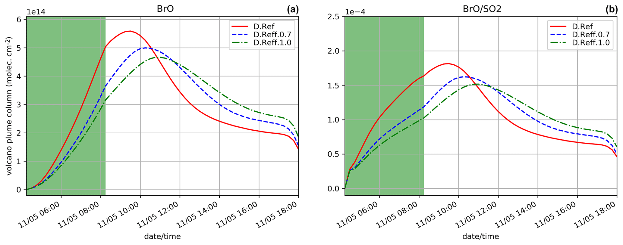
Figure 9 Similar to Fig. 4a and 4f but for the simulations testing the sensitivity to the effective radius of sulfate aerosols: D.Ref, D.Reff.0.7 and D.Reff.1.0.

5.3.3 Sensitivity to the effective radius

Two simulations test the sensitivity to the choice of the effective radius of sulfate aerosols: D.Reff.0.7 and D.Reff.1.0 with R_eff = 0.7 and 1.0 µm, respectively, instead of 0.3 µm in D.Ref. The time evolution of BrO partial column concentrations and $\mathrm{BrO}/{\mathrm{SO}}_{\mathrm{2}}$ is shown in Fig. 9. Increasing R_eff gives lower BrO with $\mathrm{BrO}/{\mathrm{SO}}_{\mathrm{2}}$ maximum occurring later. R_eff is used to define the total surface of aerosols, which is one of the parameters of the heterogeneous reaction rates (Reactions R5a, R5b and R6). For a defined sulfuric acid concentration, assuming a larger effective radius leads to a smaller total aerosol surface and therefore to lower heterogeneous reaction rates (see Supplement for more detail). This explains that BrO net production is slower as R_eff increases, leading to less HBr, ozone and NO_x depletion (not shown). This is consistent with results of Fig. 7a for the D.Emis.Sulf2 showing earlier and higher BrO and $\mathrm{BrO}/{\mathrm{SO}}_{\mathrm{2}}$ maxima with respect to D.Ref. In D.Emis.Sulf2 we assume twice as much primary sulfate concentrations compared to D.Ref, leading to an increase in the total surface of aerosols and thus to a more efficient production of BrO via higher rate constants of the heterogeneous reactions.

Compared to the plume parameterisation simulations (Sect. 5.2.2), the time evolution of BrO and $\mathrm{BrO}/{\mathrm{SO}}_{\mathrm{2}}$ in D.Reff.0.7 is close to D.Plume.0.1, whereas D.Reff.1.0 gives a lower maximum in BrO. This shows that the choice of R_eff can be even more important than the use of the plume parameterisation.

5.3.4 Sensitivity to eruption height

D.Alt.9.5 and D.Alt.7.5 simulations test the sensitivity of the results to the top altitude of the eruptive emissions, 9500 and 7500 m, respectively, instead of 8500 m for D.Ref. Note that for these tests, the figure for $\mathrm{BrO}/{\mathrm{SO}}_{\mathrm{2}}$ is not provided since the number of model levels used to calculate the partial columns on the emission levels vary and thus the column of SO₂ is not comparable between the experiments because of the background profile of SO₂.

Figure 10 shows that when the top altitude increases, the maximum of BrO occurs a bit later (1 h) and with slightly lower values (0.3 × 10¹⁴ $\mathrm{molec}.{\mathrm{cm}}^{-\mathrm{2}}$ difference). This is because at the model levels where most of the emissions are set (top third part of the profile), the concentrations of oxidants are lower at higher altitudes, leading to a lower BrO production. Here, the vertical variation of the concentrations of oxidants is the main driver of the changes of the bromine cycle efficiency. Thus, injection altitude is shown to be an important parameter.

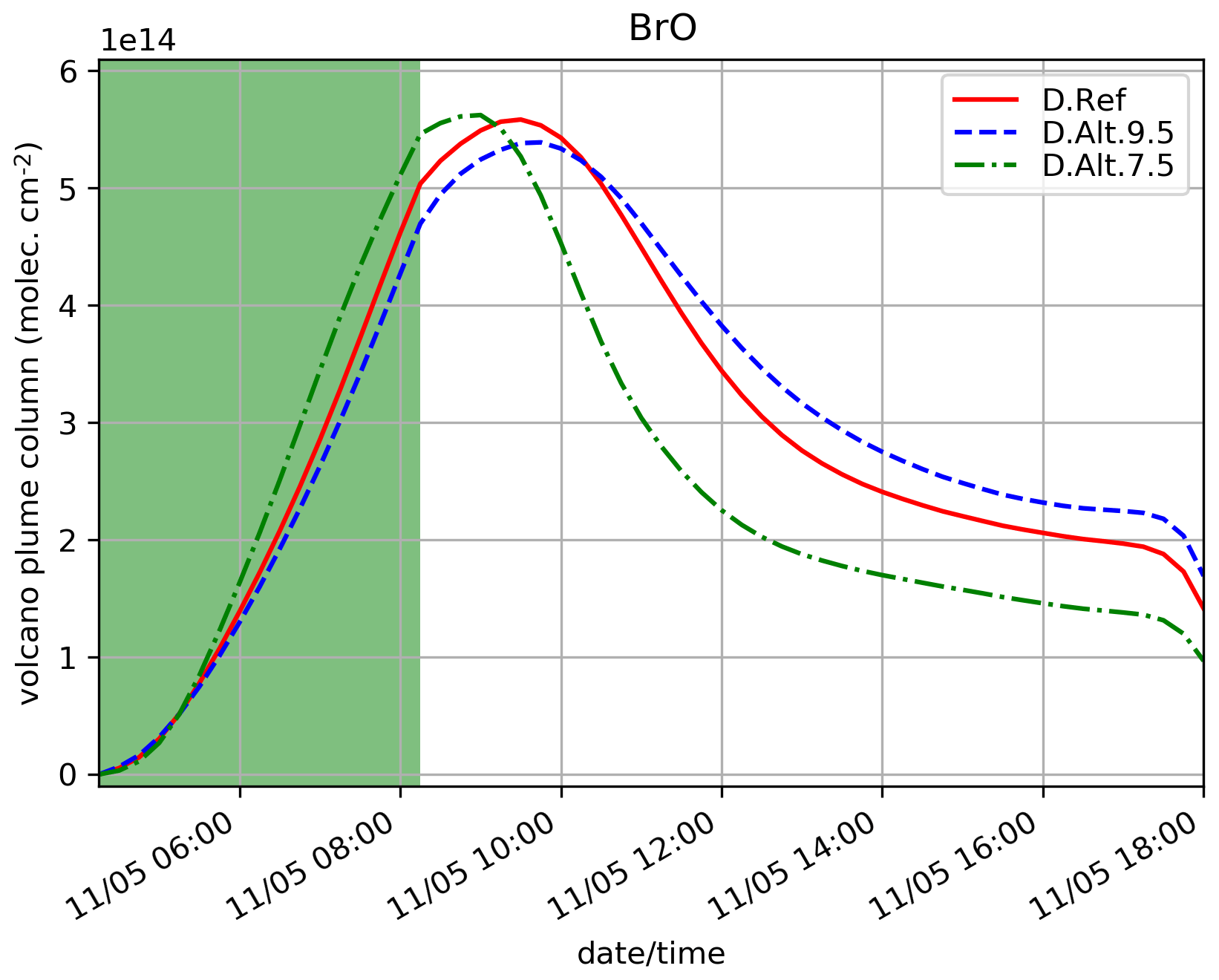
Figure 10 Similar to Fig. 4a but for the simulations testing the sensitivity to the height of the emissions: D.Ref, D.Alt.9.5 and D.Alt.7.5. Here, the quantities are integrated vertically on the emission levels: 3300–8500 m for D.Ref, 3330–9500 m for D.Alt.9.5 and 3300-7500 m for D.Alt.7.5.

Table 5 Summary of the influence of the plume parameterisation on BrO.

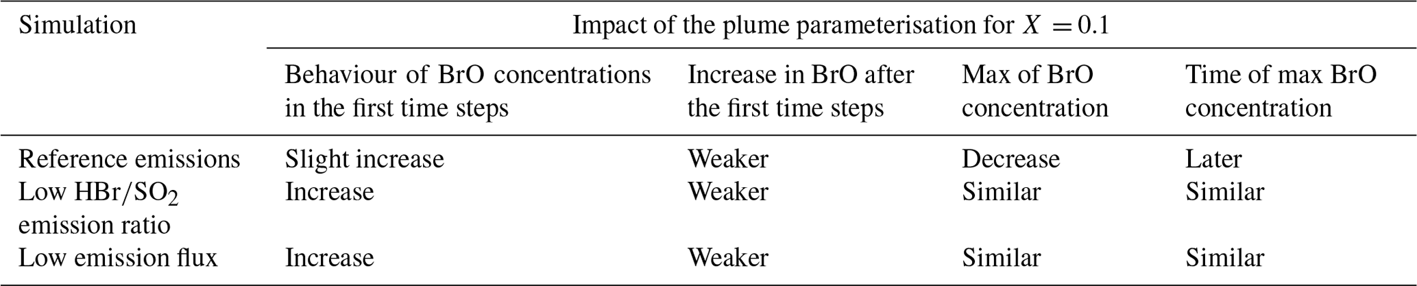
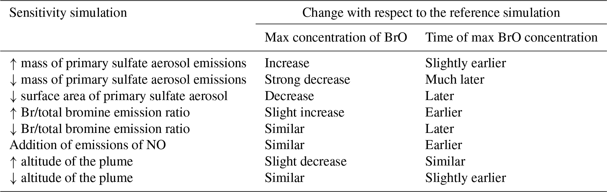
Table 6 Summary of the influence of the emission composition and plume altitude on BrO.

6 Conclusion

The formation of BrO in volcanic plumes is important for the budget, atmospheric fate and impacts of volcanic bromine emissions. From the volcanic emissions of HBr, BrO is formed in volcanic plumes via the bromine explosion cycle. This reactive bromine chemistry can have impacts far from its source as shown by the regional modelling study of Jourdain et al. (2016), the only study at the regional scale that was previously published. The present paper has the general objective to prepare the implementation of volcanic halogen chemistry in the 3D chemistry-transport model MOCAGE for regional and global simulations. More precisely, the main aim of the paper is to evaluate if the halogen chemistry developed in MOCAGE is able to produce a realistic bromine partition at a typical MOCAGE 3D model grid size. The secondary aim was to address the “plume” effect (i.e. concentrated volcanic emissions) on the chemistry processing, in particular on the bromine partitioning.

For this, the 1D version of MOCAGE is used to study the time evolution up to 20 h of a volcanic eruption containing halogen compounds. The 1D framework allows us to make a large series of sensitivity tests on different parameters.

The 1D simulations were initialised from a MOCAGE 3D simulation with a resolution of 0.5^∘ longitude × 0.5^∘ latitude (an intermediate resolution for regional and global MOCAGE applications). The MOCAGE chemical scheme was modified to account for the halogen cycle in volcanic plumes based on recent modelling studies (mainly Surl et al., 2021). The case study is the 4 h eruption of Mt Etna that occurred on 10 May 2008. In this paper, we do not aim at making a detailed analysis of the eruption but to test the volcanic chemistry scheme implemented in the 1D model on a plausible case study whose results are assessed with respect to the literature.

The results (and sensitivity studies, outlined below) are in general agreement with previous model and observation studies of volcanic plume halogen chemistry. The halogen chemistry developed in MOCAGE 1D and based on previous studies is able to produce a realistic bromine partitioning during daytime and the following morning when BrO was observed (Hörmann et al., 2013). During night-time, the bromine explosion stops because there is no photolysis leading to bromine being mainly stored in the form of Br₂ and BrCl reservoirs as expected. Additionally, to evaluate the effect on the bromine cycle of the assumption that chemical species are homogeneously distributed within MOCAGE grid box while the typical size of a volcanic plume at its early stage is much smaller, we tested a simple plume parameterisation based on Grellier et al. (2014). For this, a plume box is defined as a small box within the model box (plume box volume = $\mathrm{1}/\mathrm{400}$ model box volume) in which all the emissions are injected. We upgraded this parameterisation to make it more realistic by implementing mixing between the plume box and the model box continuously during and after the eruption. The results show that the use of this plume parameterisation slightly slows down BrO formation and its maximum concentration when the dilution decreases. The results of the plume parameterisation reflect the important control of oxidants on BrO formation (which in turn depletes atmospheric oxidants). They are consistent with the previously reported observed and modelled decrease in $\mathrm{BrO}/{\mathrm{SO}}_{\mathrm{2}}$ in the core of volcanic plumes where there are less oxidants than at the edge of the plume (Bobrowski et al., 2007; Roberts et al., 2018). Because night comes just after the end of the eruption and stops BrO production before being complete, we also run simulations starting the eruption at the beginning of the day on 11 May at 04:15 UTC (D. simulations). Findings from the daytime results with and without the plume parameterisation are fully consistent with the simulations including night (N. simulations), in terms of partitioning between halogen species, e.g. BrO, Br, HOBr and the role of oxidants.

Apart from the issue of spatial resolution, there are other sources of uncertainties in the modelling of halogen-rich volcanic plumes. Previous studies showed that the quantity and composition of the emissions used as input in the model are important. We first tested a lower total $\mathrm{bromine}/{\mathrm{SO}}_{\mathrm{2}}$ emission ratio (respectively a lower emission flux for all species) giving a more (respectively a less) efficient BrO production. These results are consistent with the literature. Note that for these two sensitivity simulations, the impact of applying the plume parameterisation is more important than in the reference simulation and leads to an increase in the BrO/total bromine ratio in the first hour of simulation. Secondly, we tested the sensitivity of the model to the emission, including species formed near the vent at very high temperature when magmatic air first mixes with atmospheric air. We show from sensitivity simulations on emitted Br and primary sulfate that both are important for a rapid BrO production, but primary sulfate aerosols are more important because they are needed for the heterogeneous reactions which are dominant in the bromine explosion. We also run a test adding NO emissions, as assumed in several previous studies. In this case, the $\mathrm{BrO}/{\mathrm{SO}}_{\mathrm{2}}$ increase is slower compared to the reference in the first hour but then gives a more efficient net production of BrO (higher $\mathrm{BrO}/{\mathrm{SO}}_{\mathrm{2}}$ ratio).

Sensitivity tests on the choice of the effective radius for the sulfate aerosols and of the top altitude of the plume highlight that these parameters are important for the bromine cycle because of the role of aerosols in the heterogeneous chemistry and of the vertical variability of oxidant concentrations available for the bromine cycle, respectively. Compared to the plume parameterisation on the bromine cycle, the impacts of the other sensitivity tests are at least comparable and sometimes more important. Knowing that there are large uncertainties on emission composition, R_eff and sometimes on the plume altitude, we find that the plume parameterisation is not the model setting that will be most important in MOCAGE 3D global/regional simulations. This parameterisation tends to slightly delay and weaken BrO net production for the emissions of the reference simulation, with similar results for different plume parameterisation settings. It is possible to achieve a similar behaviour with a larger R_eff and/or lower primary sulfate concentrations and/or lower $\mathrm{Br}/\mathrm{HBr}$ ratio in the emission (see summary Tables 5 and 6). In the case of a lower emission flux and of lower total $\mathrm{bromine}/{\mathrm{SO}}_{\mathrm{2}}$ ratio, the plume parameterisation tends to increase the BrO/total bromine ratio in the first hour of simulation. A similar effect could be simulated by using higher primary sulfate concentrations and/or the $\mathrm{Br}/\mathrm{HBr}$ emission ratio.

The findings of this study using MOCAGE 1D have recently been used to inform the design of MOCAGE 3D simulations in a case study of the impact of halogen emissions from the Mount Etna eruption that occurred around Christmas 2018 over the Mediterranean basin (Narivelo et al., 2023). These relevant findings are the following: (i) the chemistry developed is suitable to represent halogen chemistry in volcanic plumes, (ii) the plume parameterisation is not worth the additional computational cost in MOCAGE 3D, and (iii) the initial plume composition and primary sulfate aerosol are key uncertainties that need careful investigation.