the Creative Commons Attribution 4.0 License.
the Creative Commons Attribution 4.0 License.
 | 17 May 2023
Long-term evaluation of surface air pollution in CAMSRA and MERRA-2 global reanalyses over Europe (2003–2020)
Aleksander Lacima
Hervé Petetin
Albert Soret
Dene Bowdalo
Oriol Jorba
Zhaoyue Chen
Raúl F. Méndez Turrubiates
Hicham Achebak
Joan Ballester
Carlos Pérez García-Pando
Over the last century, our societies have experienced a sharp increase in urban population and fossil-fuelled transportation, turning air pollution into a critical issue. It is therefore key to accurately characterize the spatiotemporal variability of surface air pollution in order to understand its effects upon the environment, knowledge that can then be used to design effective pollution reduction policies. Global atmospheric composition reanalyses offer great capabilities towards this characterization through assimilation of satellite measurements. However, they generally do not integrate surface measurements and thus remain affected by significant biases at ground level. In this study, we thoroughly evaluate two global atmospheric composition reanalyses, the Copernicus Atmosphere Monitoring Service (CAMSRA) and the Modern-Era Retrospective Analysis for Research and Applications v2 (MERRA-2), between 2003 and 2020, against independent surface measurements of O3, NO2, CO, SO2 and particulate matter (PM; both PM10 and PM2.5) over the European continent. Overall, both reanalyses present significant and persistent biases for almost all examined pollutants. CAMSRA clearly outperforms MERRA-2 in capturing the spatiotemporal variability of most pollutants, as shown by generally lower biases (all pollutants except for PM2.5), lower errors (all pollutants) and higher correlations (all pollutants except SO2). CAMSRA also outperforms MERRA-2 in capturing the annual trends found in all pollutants (except for SO2). Overall, CAMSRA tends to perform best for O3 and CO, followed by NO2 and PM10, while poorer results are typically found for SO2 and PM2.5. Higher correlations are generally found in autumn and/or winter for reactive gases. Compared to MERRA-2, CAMSRA assimilates a wider range of satellite products which, while enhancing the performance of the reanalysis in the troposphere (as shown by other studies), has a limited impact on the surface. The biases found in both reanalyses are likely explained by a combination of factors, including errors in emission inventories and/or sinks, a lack of surface data assimilation, and their relatively coarse resolution. Our results highlight the current limitations of reanalyses to represent surface pollution, which limits their applicability for health and environmental impact studies. When applied to reanalysis data, bias-correction methodologies based on surface observations should help to constrain the spatiotemporal variability of surface pollution and its associated impacts.
- Article
(12710 KB) - Full-text XML
-
Supplement
(21880 KB) - BibTeX
- EndNote


In the last 2 decades, reanalyses have become a very powerful tool in modern Earth sciences, as they combine both model- and observation-based information to provide physically consistent data of land, ocean and atmospheric variables with continuous spatial and temporal coverage. In the field of atmospheric composition, different reanalysis products are available at global scale, including the Copernicus Atmosphere Monitoring Service reanalysis (CAMSRA; Inness et al., 2019), produced by the European Centre for Medium-Range Weather Forecasts (ECMWF), and the Modern-Era Retrospective Analysis for Research and Applications v2 (MERRA-2; Gelaro et al., 2017; Randles et al., 2017; Buchard et al., 2017a), produced by the National Aeronautics and Space Administration's (NASA) Global Modeling and Assimilation Office (GMAO). Both products assimilate a variety of space-based remote sensing observations (mostly total and tropospheric columns) obtained from a growing fleet of satellites measuring reactive gases such as ozone (O3), nitrogen dioxide (NO2) or carbon monoxide (CO), as well as aerosol optical depth (AOD). Such an extensive data assimilation of satellite observations is crucial for reducing the biases related to erroneous emission forcings and/or overly coarse representations of the physical and chemical processes that occur in the atmosphere. Data assimilation helps to better constrain the spatiotemporal variability and long-term trends of the most important chemical compounds, providing a physically consistent view of the Earth's atmospheric composition.
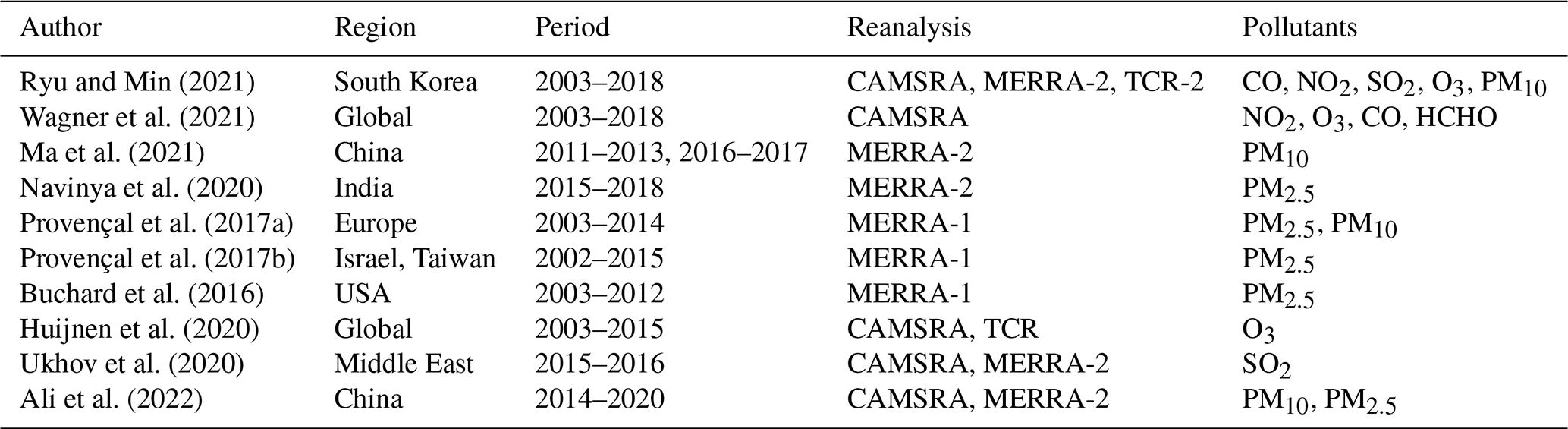
Considering the strong interest of atmospheric composition reanalyses in a variety of applications (e.g. climatological studies, initial and/or boundary conditions for regional-scale modelling systems, air pollution impact assessment, and health studies), it is crucial to characterize the strengths and limitations of these global products, in particular at the surface, as no in situ chemical observations are assimilated. The most recent studies evaluating the CAMSRA and/or MERRA-2 reanalysis at ground level are indicated in Table 1, highlighting the limited effort that has been made so far to evaluate and inter-compare these reanalysis products against in situ surface measurements.
The main findings of this more recent literature are briefly outlined here. Ryu and Min (2021) found significant and persistent biases in all the pollutants examined over South Korea, with CAMSRA outperforming MERRA-2 in all cases except for SO2. At global scale, Wagner et al. (2021) showed that CAMSRA provides an overall accurate representation of reactive gases over time and highlighted the key role played by satellite data assimilation in improving atmospheric composition reanalysis products. Both these two previous studies analyse a wide range of aerosols and reactive gases and cover the most extensive period possible at the time, 2003–2018, which is limited by the start of CAMSRA in 2003. Ma et al. (2021) found persistent negative biases in particulate matter (PM10) concentration over mainland China in MERRA-2 for the periods 2011–2013 and 2016–2017, with better performance during summer. Their results also showed a significant improvement when including nitrate compounds. Navinya et al. (2020) found a systematic underestimation of PM2.5 concentration in MERRA-2 over India for the period 2015–2018. Huijnen et al. (2020) found limited surface O3 biases when evaluating CAMSRA over Europe (−1.8 ppbv). Ukhov et al. (2020) evaluated surface SO2 for 2015–2016 over three cities in the Middle East and found a large underestimation for MERRA-2, while CAMSRA showed both moderate negative and positive biases. Lastly, Ali et al. (2022) evaluated PM over the period 2014–2020 in China and found significant over- and underestimations both for CAMSRA and MERRA-2.
Ryu and Min (2021)Wagner et al. (2021)Ma et al. (2021)Navinya et al. (2020)Provençal et al. (2017a)Provençal et al. (2017b)Buchard et al. (2016)Huijnen et al. (2020)Ukhov et al. (2020)Ali et al. (2022)Table 1Review of recent studies evaluating the CAMSRA and/or MERRA-2 reanalysis at the surface using in situ observations.
Our study evaluates CAMSRA and MERRA-2 against independent surface in situ measurements over the period 2003–2020, focusing on the European continent, a region still poorly covered by past evaluation studies (Table 1). It considers all major pollutants with recognized harmful effects on human health and sufficient observational data available at the surface, namely O3, NO2, CO, SO2, PM10 and PM2.5. The motivation behind this study arose in the context of the European Research Council (ERC) project EARLY-ADAPT (https://early-adapt.eu/, last access: 15 December 2022), in which framework a pioneer health database is currently being collected over Europe to investigate the time-varying health effects of climate and air pollution, and thus shed light onto the early adaptation response to climate change in the field of human health. This impact will be quantified by fitting epidemiological models on historical local health, climate and air pollution data, which thus requires a long-term (multi-decadal) air quality database of the most harmful pollutants at daily scale and over the entire European domain. Despite their relatively coarse spatial resolution, which is the counterpart to a sufficiently long-term coverage, global-scale atmospheric composition reanalyses provide highly valuable information, though remain subject to biases and errors both in terms of spatial, seasonal and intra-annual variability and regarding long-term trends. It is worth mentioning here that the CAMS regional reanalysis (Marécal et al., 2015), focused on Europe, assimilates surface in situ observations and provides air pollution fields at a finer spatial resolution than CAMSRA but only over a limited period of time (2014–2018), for which reason we focus here on the global reanalysis.
In Sect. 2, we introduce the data (Sect. 2.1) and provide details on the different methods employed for their analysis (Sect. 2.2). Results are presented and discussed in Sect. 3 and summarized in Sect. 4.
In this section we briefly describe our observational and reanalysis datasets, while providing details on the different statistical methods employed for their analysis. Throughout this work, square brackets, [], are used to indicate the concentration or mixing ratio of a chemical compound (e.g. [O3] = O3 mixing ratio, [PM10] = PM10 concentration) measured in parts per billion (ppbv) for reactive gases and in µg m−3 for aerosols. Nonetheless, the term concentration is used for the sake of simplicity when reactive gases are mentioned together with aerosols.
2.1 Data
Our model data come from two global atmospheric composition reanalyses, CAMSRA and MERRA-2, whose main characteristics are summarized in Table 2. The reanalyses are evaluated against surface in situ measurements obtained from two European Environment Agency (EEA) databases, AirBase, for the period 2003–2012 (EEA, 2014), and AQ e-Reporting (EEA, 2018), for the period 2012–2020. No significant inconsistencies are expected between AirBase and AQ e-Reporting given that stations included in both databases are obtained from the same network. Though stations may be renamed, relocated or even removed with time, this is not expected to significantly affect our data given the large number of stations considered and the continuous addition of new stations into the network throughout the whole period of 2003–2020.
2.1.1 CAMSRA
Produced by ECMWF, the CAMS global atmospheric composition reanalysis consists of three-dimensional time-consistent atmospheric composition fields that include chemical species, aerosols and greenhouse gases (GHGs) and currently covers a temporal period extending from 2003 to mid-2021. The reanalysis started in 2003, when space-based observational measurements, retrieved from a myriad of instruments on board Envisat, Terra, Aura, MetOp and POES satellites, became available. The latest CAMSRA version was produced in cycle 42R1 of ECMWF's Integrated Forecasting System (IFS) using 4DVar data assimilation of satellite measurements, including O3, NO2, CO and AOD. This IFS cycle includes the modified Carbon Bond 2005 Chemical Mechanism (CB05), which serves as the tropospheric chemistry scheme of the reanalysis (Flemming et al., 2015). Anthropogenic emissions come from the MACCity inventory data (Granier et al., 2011) for the period 2003–2010, and from 2010 onwards they are derived according to the representative concentration pathway of 8.5 W m−2 (RCP8.5). Biomass burning emissions are obtained from the Global Fire Assimilation System (GFAS) v1.2 (Kaiser et al., 2012), whereas monthly mean biogenic volatile organic compound (VOC) emissions are computed with the Model of Emissions of Gases and Aerosols from Nature (MEGAN) using MERRA-2 reanalysed meteorology (Sindelarova et al., 2014). Meteorological observations are assimilated as in ERA5 (Hersbach et al., 2020).
CAMSRA has a horizontal resolution of approximately 80 km (similar to a regular 0.75∘ × 0.75∘ latitude–longitude grid), with atmospheric composition fields being available only in grid-point space. Its vertical resolution consists of 60 hybrid sigma/pressure model levels, with the top of the first level at 10 m above ground and the top level located at 0.1 hPa. CAMSRA products are available at a temporal resolution of 3 h, including 3-hourly analysis fields and 3-hourly forecast fields. The biases present in the different atmospheric composition satellite-retrieved datasets employed to build CAMSRA are corrected through a variational bias-correction scheme (Dee and Uppala, 2008). For a more thorough and detailed description of CAMSRA we direct the reader to Inness et al. (2019) and Wagner et al. (2021).
In CAMSRA, both PM10 and PM2.5 are directly available and do not require to be reconstructed from its separate aerosol compounds, which include black carbon (BC), organic carbon (OC), organic matter (OM), sulfate (SO4), sea salt and dust. Both PM fields were downloaded directly without any reconstruction or modification, though they are originally reconstructed from the following formulas:
where ρ is the air density; SS1 and SS2 the sea salt; DD1, DD2 and DD3 the dust; OM1 and OM2 the organic matter; BC1 and BC2 the black carbon; and SU1 the aerosol sulfate mass mixing ratios (with 1/2/3 referring to the aerosol bins, from smallest to largest). The factor 4.3 is applied to convert the model sea salts, expressed at 80 % relative humidity in the model (see Reddy et al., 2005), into dry mass mixing ratios. However, it is worth mentioning that to the best of our knowledge, this correction might need to be revisited in the future to also account for the change of size of the sea salt particles (as mentioned on the CAMS scientific user forum: https://confluence.ecmwf.int/display/CUSF/PM10+and+PM25+global+products, last access: 25 November 2022). Notably, aerosol nitrates are, at this time, not included in the reanalysis, which could in principle lead to significant underestimations in regions where nitrates represent an important part of total aerosol concentration. Although in practice, the assimilation of AOD observations (that evidently integrate all the aerosol compounds) is expected to reduce these biases. Within OM, secondary organic aerosols (SOAs) of anthropogenic origin are parameterized according to Spracklen et al. (2011), based on MACCity CO emissions. A detailed description of the aerosol scheme employed in CAMSRA can be found in Morcrette et al. (2009).
(Hersbach et al., 2020)Rienecker et al., 2008Molod et al., 2012(Flemming et al., 2015)Chin et al., 2002Colarco et al., 2010(Granier et al., 2011)Diehl et al., 2012(Janssens-Maenhout et al., 2011; Janssens-Maenhout, 2011)(Kaiser et al., 2012)(Duncan et al., 2003)(Randerson et al., 2006)(Darmenov and da Silva, 2015)(Sindelarova et al., 2014)(Guenther et al., 1995)Diehl et al., 2012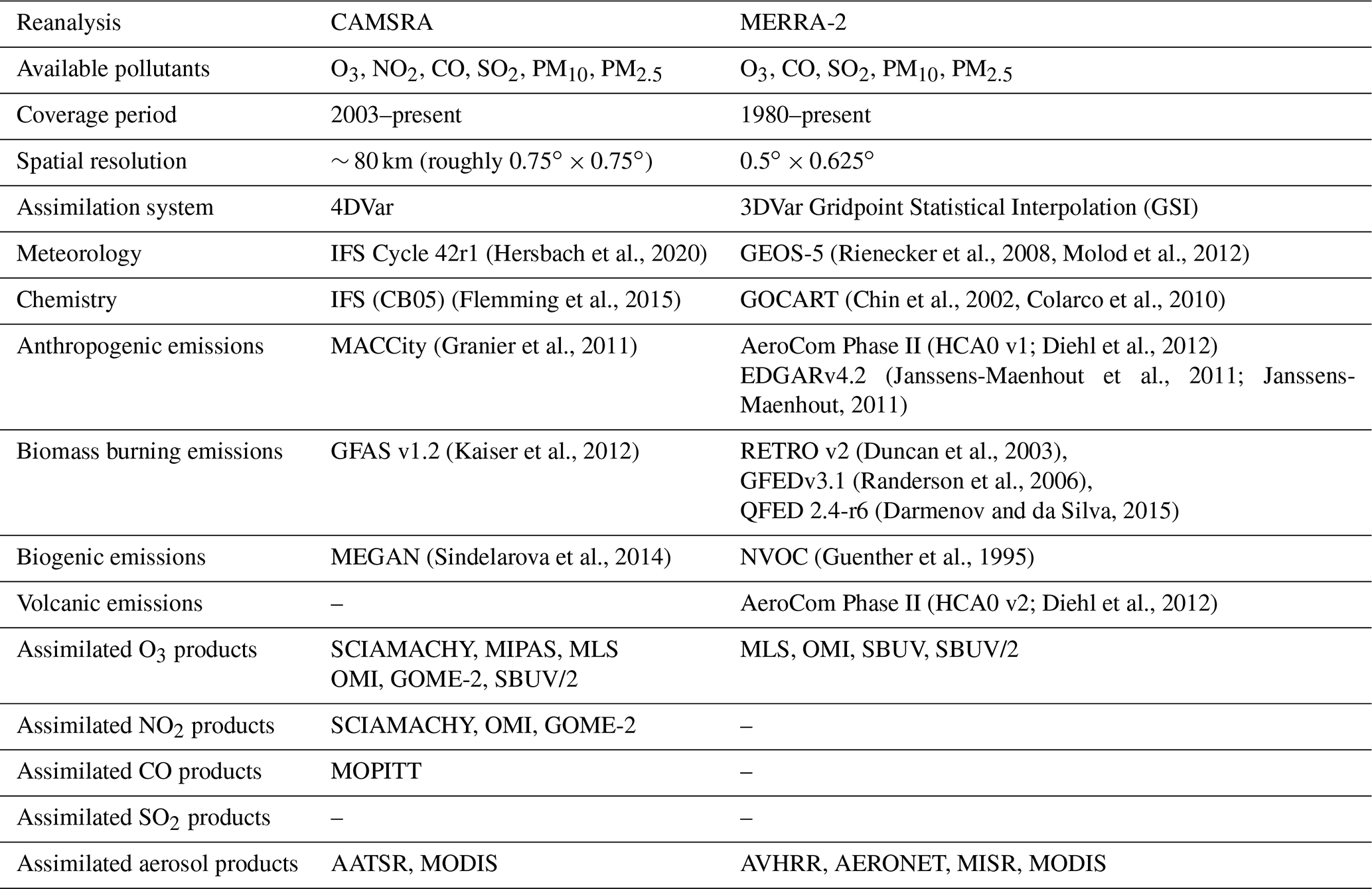
2.1.2 MERRA-2
Developed by NASA’s GMAO, the MERRA-2 atmospheric composition reanalysis is based on the Goddard Earth Observing System v5 (GEOS-5) atmospheric model. It is important to note at this stage that, in contrast with CAMSRA, which aims to simulate all major chemical compounds present in the atmosphere, the MERRA-2 reanalysis, despite being the first atmospheric composition reanalysis that couples chemistry to global atmospheric circulation, focuses mainly on aerosols. Therefore, aside from meteorological data, only AOD observations and O3 columns are assimilated in MERRA-2, based on both measurements from Terra, Aura, MetOp and POES satellites, and – unlike in CAMSRA – surface-based observations from the Aerosol Robotic Network (AERONET). Anthropogenic sulfate, black carbon (BC) and primary organic matter (POM) emissions are obtained from AEROsol COMparisons between Observations and Models (AeroCom) Phase II (HCA0 v1; Diehl et al., 2012). Anthropogenic SO2 emissions are taken from the Emissions Database for Global Atmospheric Research (EDGAR) v4.2, developed by the European Commission (Janssens-Maenhout et al., 2011; Janssens-Maenhout, 2011), whereas volcanic SO2 is retrieved from AeroCom Phase II (HCA0 v2; Diehl et al., 2012). CO is simulated by the GEOS-5 modelling system. Sea salt and dust emissions, both composed of five non-interacting size bins, are wind-driven. Aerosol chemistry is reproduced with a version of the Goddard Chemistry Aerosol Radiation and Transport (GOCART; Chin et al., 2002, Colarco et al., 2010) model, which simulates the processes, interactions, sources and sinks of the different chemical compounds included in MERRA-2, with the exception of O3 and CO.
MERRA-2 currently covers a temporal period extending from 1980 to mid-2021. The reanalysis was produced using 3DVar data assimilation of AOD and several other meteorological fields. MERRA-2 uses cubed-sphere horizontal discretization, which serves to mitigate grid spacing singularities that appear in regular Gaussian grids, at an approximate resolution of 0.5∘ × 0.625∘ (∼ 50 km) and has 72 hybrid-eta model levels from the surface, with the first level reaching 58 m above ground to the top at 0.01 hPa. MERRA-2 includes 1-hourly and 3-hourly analysis fields for its aerosol diagnostics and meteorological data. For a more thorough and detailed description of MERRA-2 we direct the reader to Gelaro et al. (2017) and Randles et al. (2017).
Designed primarily for research focused on aerosols, the MERRA-2 reanalysis dataset also provides data of the most important trace gases, including O3, CO and SO2 (with only NO2 being unavailable). In MERRA-2, both PM10 and PM2.5 need to be reconstructed from the available aerosol chemical compounds, which include organic carbon (OC), black carbon (BC), dust (DS), sea salt (SS) and sulfate (SO4). In this study, the PM10 and PM2.5 concentrations are computed as follows:
The 1.375 factor applied to [SO4] is used here to convert sulfate into ammonium sulfate (assuming full neutralization). The 1.8 factor applied to [OC] accounts for other organic compounds found in organic matter (OM). In recent literature, Eq. (2a) and (2b) are the most frequently used to reconstruct the PM fields. Equation (2a) is used by Provençal et al. (2017b) and also by Ma et al. (2021), though with an additional term to account for aerosol nitrates in the latter. Equation (2b) is used by Provençal et al. (2017a, b) and by Ryu and Min (2021), where it is also employed to reconstruct [PM10] by multiplying it with a measurement-based [PM10][PM2.5] ratio of 1.75 (computed over the period 2003–2018). Note also that there are large uncertainties in the [OM][OC] ratio, as it varies in time and space, and other studies have chosen a different value (e.g. 1.4 in Buchard et al., 2016 and Buchard et al., 2017b) for this factor. Notably, nitrates are currently not available in MERRA-2, even though they can make up a considerable portion of total [PM] Aldabe et al. (2011). To overcome this limitation, some authors such as Ma et al. (2021) have introduced an additional term partly based on observations.
In our study aerosol nitrates are not included in the PM10 and PM2.5 concentration fields, neither in MERRA-2 nor in CAMSRA. The potential underestimation due to the absence of nitrates is at least partially compensated by the fact that both reanalyses assimilate total AOD observations, which corrects all PM chemical compounds proportionally and thus minimizes the biases due to the absence of aerosol nitrates.
2.1.3 Air quality observations and GHOST
The EEA observations are accessed from the Globally Harmonised Observational Surface Treatment (GHOST) initiative, a Barcelona Supercomputing Center (BSC) in-house project dedicated to the harmonization of global air pollution surface observations and its metadata, with the purpose of facilitating a greater quality of observational/model comparison in the atmospheric chemistry community. Besides the chemical concentration data originally available in the EEA databases, GHOST provides an extended set of metadata, including a variety of quality assurance (QA) flags, which is used here to eliminate doubtful, non-physical or other faulty data (see Appendix D for a detailed description of the QA filters applied here). To ensure a good temporal representativeness, only daily averages based on at least 18 hourly values (75 % threshold) are retained in our study. Given the relatively coarse spatial resolution of both reanalyses, only rural, rural–regional and rural–remote background stations of larger spatial representativeness are considered in the evaluation, thus excluding urban and suburban background stations. Traffic and industrial point source stations have also been discarded, being generally located in areas with limited air flow and close to local emission sources, which causes their pollution concentration levels to be overly driven by day-to-day variability. For information purpose, evaluation results obtained considering only urban and suburban background stations will also be briefly discussed. More information on the station classification can be found on the EEA website (https://www.eea.europa.eu/themes/air/air-quality-concentrations/classification-of-monitoring-stations-and, last access: 15 December 2022).
2.2 Methodology
Our domain of study extends from 25∘ W to 45∘ E in longitude and from 27 to 72∘ N in latitude, thus covering all of continental Europe, as well as the Canary Islands, Iceland, western/European Russia, North Africa, and the westernmost regions of the Middle East and the Caucasus. For convenience, both CAMSRA and MERRA-2 are regridded over this domain on a common regular longitude–latitude grid at a resolution of 0.2∘ × 0.2∘ (roughly 20 km) through bilinear interpolation. The (pointwise) observations are also gridded to this same resolution by averaging (at daily scale) all the stations available within a given grid cell. Compared to a pointwise-to-gridded comparison, this is expected to partly overcome the issues of spatial representativeness and spatial heterogeneity, although we acknowledge here that more sophisticated methods such as those proposed by Souri et al. (2022) (which employ geostatistical approaches by making use of semivariograms and kriging) might be worth implementing in the future. However, when considering only rural, rural–regional and rural–remote background stations, the proportion of gridded daily observations based on one single daily observation (two daily observations) is 96.1 % (3.5 %) for NO2, 95.4 % (4.4 %) for O3, 96.7 % (3.2 %) for SO2, 97.9 % (1.9 %) for CO, 91.0 % (8.5 %) for PM10 and 92.5 % (7.4 %) for (7.4 %) for PM2.5; these high percentages are explained by the presence of numerous missing values throughout the period of study. Table 3 and Fig. 1 provide some information on the observations available over our European domain during 2003–2020, in terms of both pointwise and gridded observations (the total number of observations is typically reduced by a 2–3 factor after the gridding operation). Unfortunately, in situ observations from GHOST are not available for several countries falling within the domain considered in this study, located in North Africa (e.g. Morocco, Algeria, Tunis, Libya, Egypt), Eastern Europe (e.g. Russia, Belarus, Ukraine) and the Middle East (e.g. Israel, Lebanon, Jordan, Syria), thus somewhat limiting the scope of the evaluation, particularly in terms of spatial variability and pollution hotspots.
Table 3Number of EEA background stations (S), number of gridded stations (G) and number of overall points (i.e. daily values) (N) over the period 2003–2020.
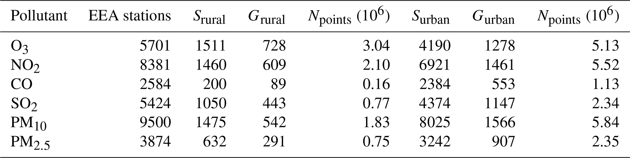
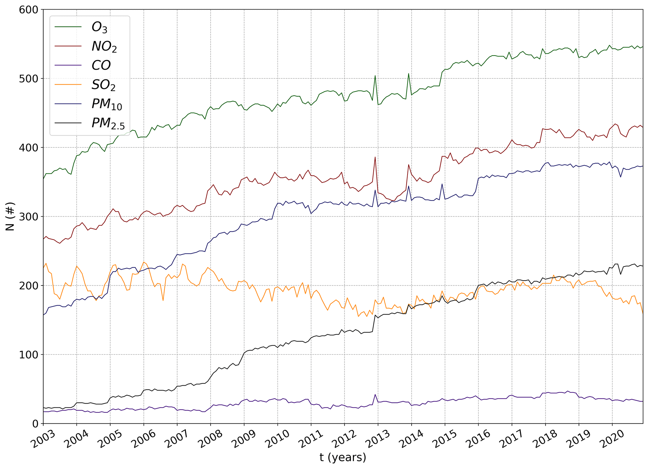
Figure 1Monthly number of rural gridded cells with available observational data for O3, NO2, CO, SO2, PM10 and PM2.5 over the period 2003–2020.
The evaluation is performed on a set of metrics including the (normalized) mean bias ((n)MB), the (normalized) root mean square error ((n)RMSE) and the Pearson correlation coefficient (PCC), defined as follows:
where mi and oi are the predicted and observed concentrations, and are their means, σm and σo are their standard deviations, and N is the number of points employed to compute the statistics (i.e. number of daily values across all stations). The index i accumulates over time (e.g. daily, monthly) at each station (i.e. gridded cell with available observations). The final value for each statistic is obtained by taking the median across all stations. The overlines in Eq. (3a)–(3e) indicate a time-averaged variable.
In this study, metrics have been calculated and presented following two different approaches: (1) with a so-called “time-and-space” approach where metrics are calculated in one step, based on all reanalysis–observation pairs available both across the entire domain (or a given country) and over the entire period 2003–2020 or (2) with a so-called “time-then-space” approach where metrics are first calculated at each station before being combined by taking the median across all stations. In this work framework, time-and-space PCC values do not correspond to spatial or temporal correlations but rather to overall spatiotemporal correlations, while time-then-space PCC values do correspond to temporal correlations, though spatially averaged.
Annual trends, based on monthly averages over the entire domain (considering only cells and days with available observations to allow for fair comparisons) and reported in Sect. 3, have been computed using seasonal Theil–Sen estimators, which account for seasonal variability. Statistical significance has been analysed through correlated seasonal Mann–Kendall trend tests, considering both seasonality and autocorrelation. For more detailed information on how the annual trends are computed we refer the reader to Appendix C. It is worth noting that trends are here computed essentially to evaluate the consistency of the reanalyses against observational data but should not be taken as a reliable estimate of real pollutant trends due to the number of stations not being constant but generally increasing throughout the period of study. Moreover, even if a station has available data over the entire period, its location can also be subject to changes over time.
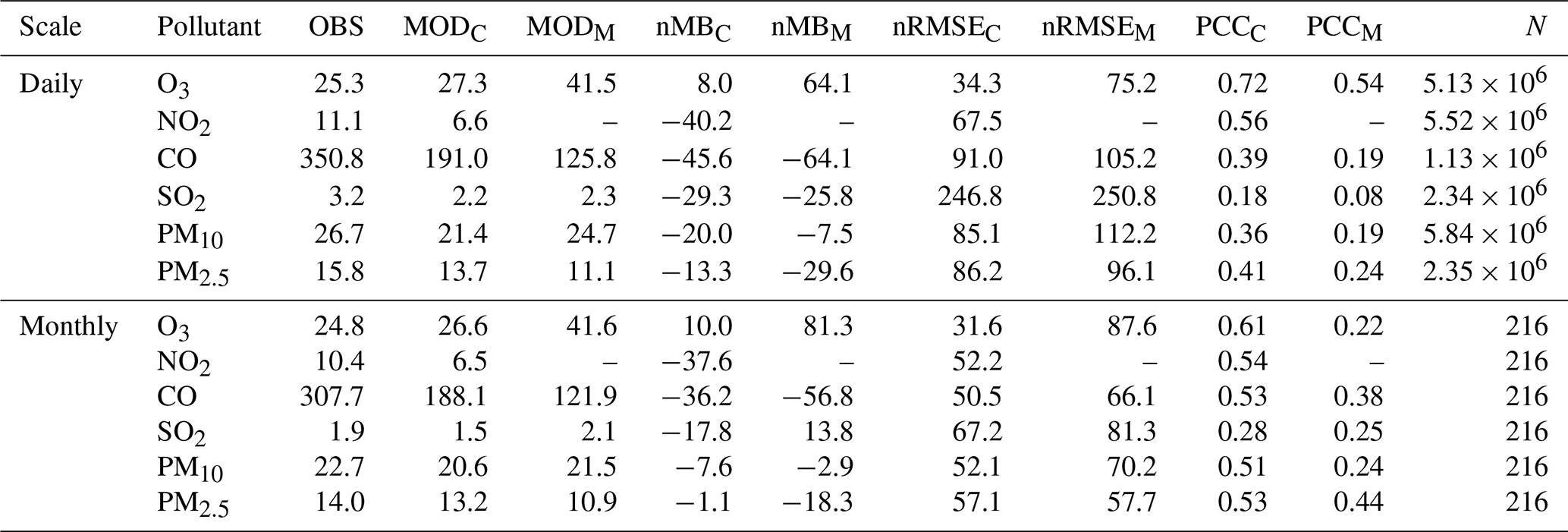
The evaluation results, alongside its analysis and discussion, are presented in this section. Overall statistics obtained over the European continent during 2003–2020 are provided in Table 4 (time-and-space approach). Annual trends are reported in Table 5 for the different pollutants.
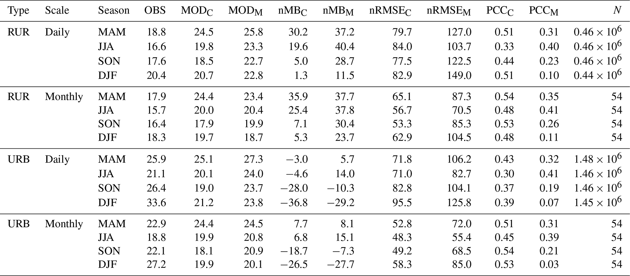
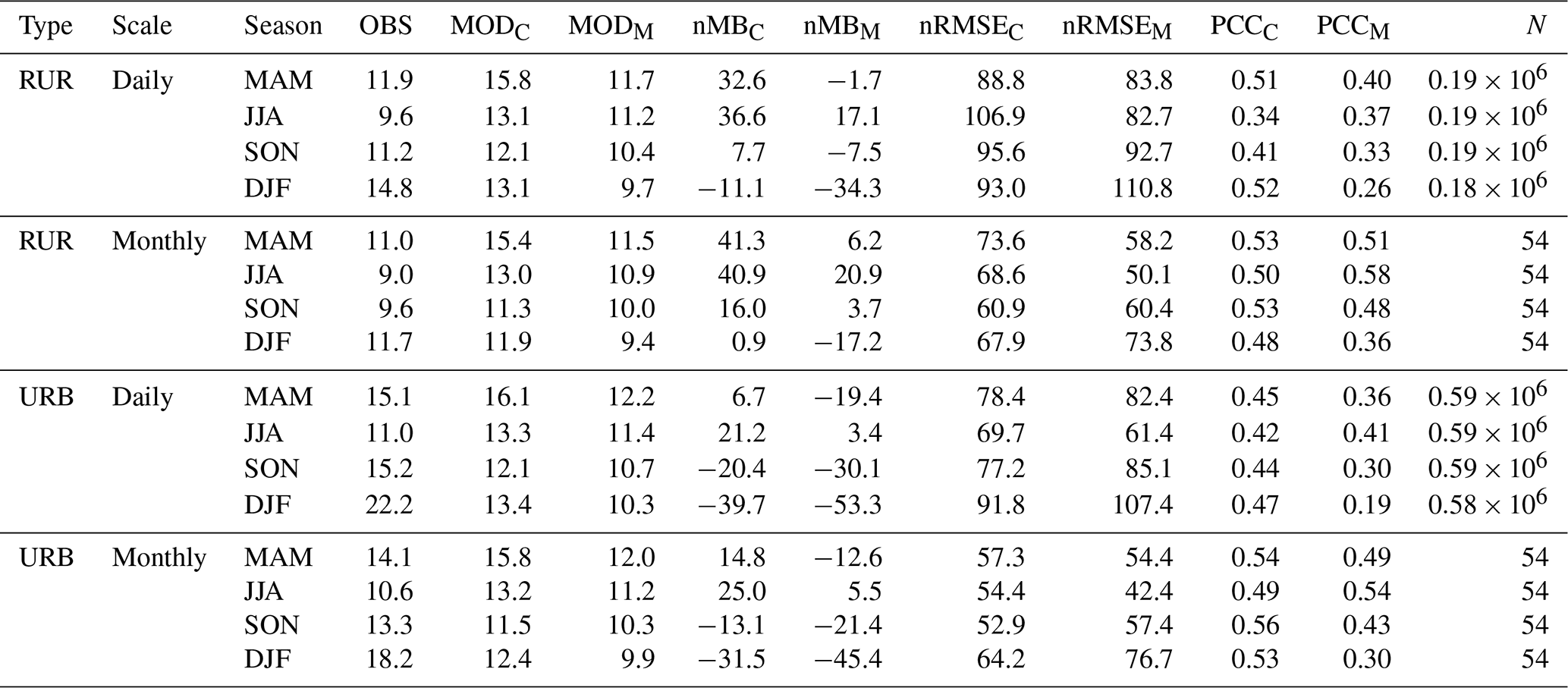
Different aspects of the evaluation results are provided for each pollutant in Figs. 2–7, including (1) monthly time series of concentrations and evaluation statistics, (2) bar plots of country-scale statistics, and (3) maps of mean concentrations (and differences between both reanalyses) over the domain. Each point in the monthly time series corresponds to the median of the monthly mean values across all individual cells with available observations over the domain. In order to highlight potential spatial differences in pollution patterns across the European continent, country-scale statistics computed over the entire time period and country area are provided for 37 European countries which either are part of or report data to the EEA, namely Albania (AL), Austria (AT), Bosnia and Herzegovina (BA), Belgium (BE), Bulgaria (BG), Switzerland (CH), Cyprus (CY), Czech Republic (CZ), Germany (DE), Denmark (DK), Estonia (EE), Greece (EL), Spain (ES), Finland (FI), France (FR), Hungary (HR), Ireland (IE), Iceland (IS), Italy (IT), Lithuania (LT), Luxembourg (LU), Latvia (LV), Montenegro (ME), North Macedonia (MK), Malta (MT), the Netherlands (NL), Norway (NO), Poland (PL), Romania (RO), Serbia (RS), Sweden (SE), Slovenia (SI), Slovakia (SK), Turkey (TR), and the United Kingdom (UK). Additional results are provided in Appendix A, including seasonal-scale statistics (Tables A1–A6) and mean monthly profiles (Figs. A1–A2) for rural (RUR) and urban (URB) background stations. Further additional results can be found in the Supplement, including overall statistics for all EEA member countries, figures such as Figs. 2–7 but for urban background stations and a visualization of different methods employed by other studies to reconstruct the PM10 concentration field in MERRA-2.
Table 4Overall statistics obtained over the period 2003–2020 across Europe for CAMSRA (subscript C) and MERRA-2 (subscript M). Statistics are shown both on a daily scale (over all cells and days in the period 2003–2020) and on a monthly scale (weight averaged by N over all median monthly values). OBS and MOD stand for observational and model concentration, respectively. Reactive gas mixing ratios are expressed in ppbv, aerosol concentrations in µg m−3 and normalized statistics in %.
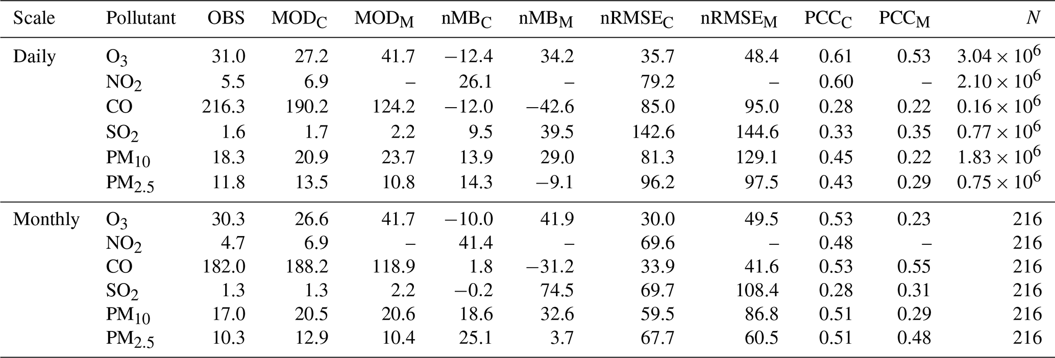
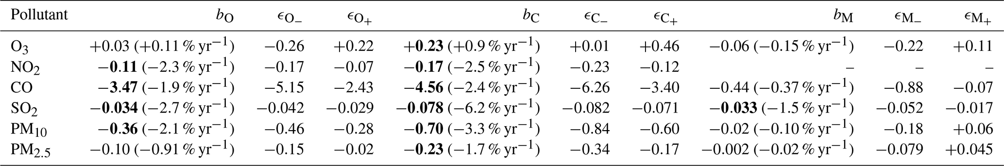
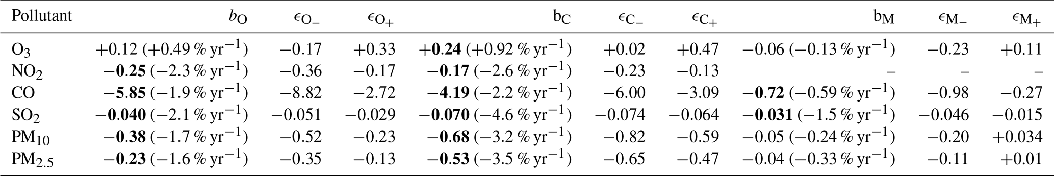
Table 5Annual trends (seasonal Theil–Sen estimators, b) over the period 2003–2020 across Europe for rural observations (subscript O), CAMSRA (subscript C) and MERRA-2 (subscript M) together with corresponding 99 % confidence intervals (ϵ−, ϵ+). Statistically significant annual trends are highlighted in bold. Trends and uncertainty ranges are expressed in ppbv yr−1 and for reactive gases and aerosols, respectively. Relative trends (normalized by the mean concentration over 2003–2020) are also indicated in parenthesis.
3.1 Ozone (O3)
Overall, CAMSRA reproduces the observed [O3] fairly well, with limited negative bias (−12 %) and reasonable error and correlation (36 % and 0.61, respectively). In comparison, MERRA-2 systematically overestimates [O3] (+34 %) and shows poorer error and correlation (48 % and 0.53, respectively). On average, observed O3 mixing ratios reach a minimum between late autumn and early winter then peak in spring and are followed by persistently high but slowly decreasing O3 levels until reaching a sharp drop in late summer (Fig. A1 in the Appendix). CAMSRA captures the seasonality of O3 reasonably well, although with negative bias during winter and early spring. Conversely, MERRA-2 substantially underestimates the seasonal amplitude (around 15 ppbv, against more than 20 ppbv in observations and CAMSRA).
Throughout the entire period, the median monthly scale nMB in CAMSRA remains below −20 %, with larger underestimations through the beginning of the period and better results during the last years. The bias displays a clear seasonal pattern, with an important winter and spring deterioration (−21 % and −16 %, respectively) but very limited biases in summer and autumn (−4 % and −1 %, respectively). Such oscillating biases have also been reported by Huijnen et al. (2020) over Europe. Regarding the other metrics, median monthly scale nRMSE in CAMSRA reaches its worst values in winter (36 %) when the PCC is conversely the best (0.71), whereas an opposite behaviour with low nRMSE and poor PCC can be observed in summer (26 % and 0.40, respectively). A strong seasonal variability is also found in MERRA-2 statistics, although limited to nMB and nRMSE, which are worst in autumn (+61 % and +67 %, respectively). While the reasonable PCC obtained over the entire dataset (0.53) is likely driven by the good ability of MERRA-2 to capture the O3 seasonality, the much lower monthly PCC values (oscillating around 0.25) suggest that MERRA-2 represents the intra-monthly variability of daily O3 mixing ratios very poorly over a large part of the domain. Nonetheless, MERRA-2 is able to reproduce the spring peak followed by a slow decrease in [O3] typically seen in European observations during summer. In contrast, CAMSRA completely misses this mid-spring O3 peak, as shown in Fig. A1. Over 2003–2020, no statistically significant annual trend (estimated as a seasonal Theil–Sen slope) of mean [O3] is observed over Europe, neither in MERRA-2 nor in the observations. However, a significant though low positive increase of +0.23 ppbv yr−1 is found in CAMSRA (Table 5), at least partly due to the aforementioned stronger underestimation of O3 during the first years of the period.
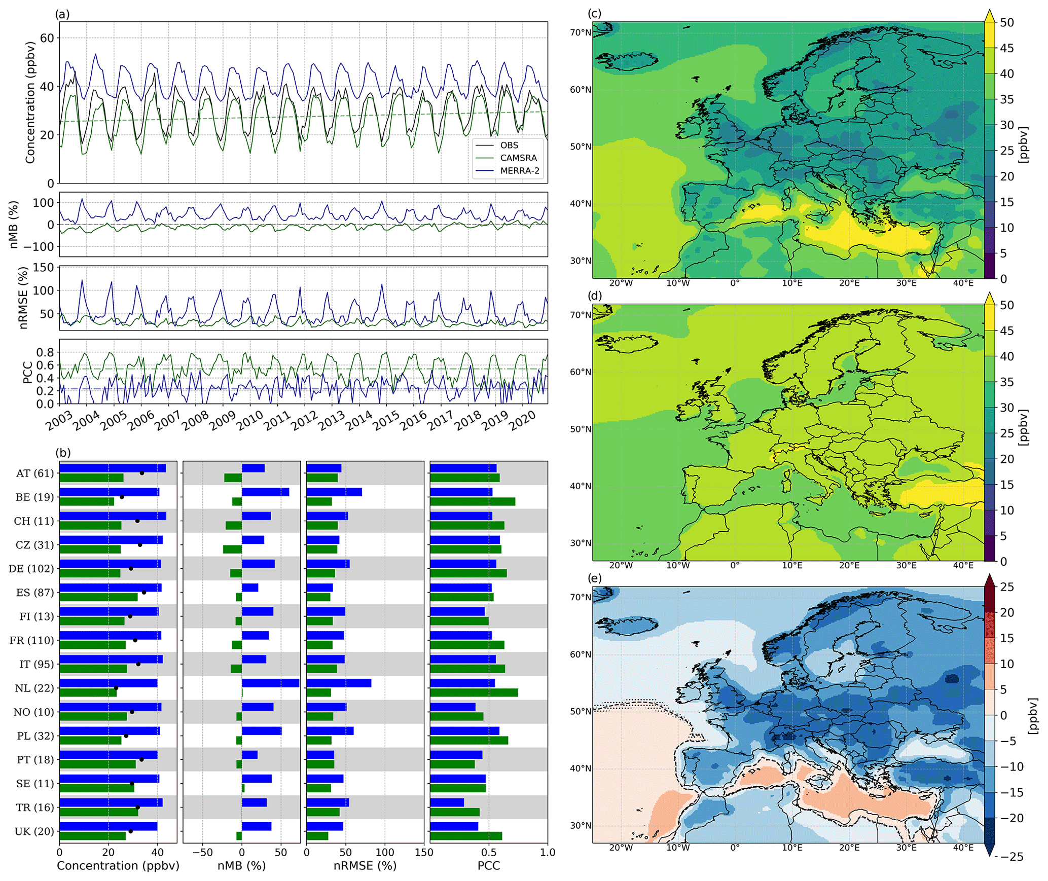
Figure 2Evaluation of O3 over Europe depicting (a) monthly time series of [O3], nMB, nRMSE and PCC over the period 2003–2020; (b) spatially averaged [O3], nMB, nRMSE, and PCC for countries with at least five cells with observations; (c) mean [O3] climatology in CAMSRA; (d) mean [O3] climatology in MERRA-2; and (e) differences in mean [O3] climatology between CAMSRA and MERRA-2. Black, green and blue colours in (a) and (b) indicate observations, CAMSRA and MERRA-2, respectively. Numbers between parentheses in (b) indicate the cells with available observations. Only PCC values in the range 0–1 are displayed in (b). Statistically significant trends, at a 99 % confidence level, are displayed in (a). Dotted areas in (e) indicate where the differences are not statistically significant at a 99 % confidence level, whereas the dashed black contour stands for a zero difference in concentration between reanalyses.
The country-level evaluation highlights how CAMSRA outperforms MERRA-2 in every single country across the European continent for every computed statistic, with the greatest differences appearing in Belgium (BE) and the Netherlands (NL) and the smallest ones in Spain (ES) and Portugal (PT). In CAMSRA the nMB remains generally negative, at around −10 %, with several countries showing virtually no bias (e.g. the Netherlands (NL), Turkey (TR) and Sweden (SE)), while MERRA-2 displays values in the range of +30 %–70 %. As for the nRMSE, in CAMSRA it remains constrained between 30 % and 50 % for all evaluated countries, whereas in MERRA-2 it generally remains close to 50 %, even surpassing this value for several countries, such as the Netherlands (NL), Poland (PL), Belgium (BE) and Turkey (TR). In most countries the PCC does not differ considerably between reanalyses, remaining in the range 0.4–0.7 and slightly higher values for CAMSRA. Despite its greater original resolution, MERRA-2 fails to capture the spatial variability of the [O3] field, with highly homogeneous mixing ratio values over land, ranging from 35 to 45 ppbv (Fig. 2d), likely a result of the lack of accurate ozone sources in the parameterized chemistry and limited sensitivity of OMI measurements to lower tropospheric ozone (note that neither MLS nor OMI provide ozone profile information in the troposphere). A wider range of assimilated products, as seen in Table 2, and more detailed gas-phase chemistry likely accounts for CAMSRA's better overall performance and greater spatial variability. Nevertheless, we expect the MERRA-2 ozone profile product to be useful for scientific studies that focus on the upper troposphere and the stratosphere, given the high correlations found by Bosilovich et al. (2015) against independent ozonesonde data at these altitudes.
Inness et al. (2019) evaluated surface O3 against the World Meteorological Office's (WMO) Global Atmosphere Watch (GAW) background stations and noticed slightly higher negative biases in winter (with modified nMB down to −40 %), though based on a different and smaller set of stations (45 GAW stations against 1511 EEA rural background stations gridded into 728 cells here). Over 2003–2018, Wagner et al. (2021) evaluated CAMSRA surface O3 mixing ratios against the European Monitoring and Evaluation Programme's (EMEP) observations, finding typically negative modified normalized mean biases (MNMBs) within −30 % in winter (driven by underestimated O3 mostly at midlatitudes) but positive ones in summer and autumn up to +15 %. Such an oscillating bias is in good agreement with our results over the European continent. Although satellite O3 measurements are extensively assimilated in CAMSRA (11 space-based O3 products included), Wagner et al. (2021) already demonstrated their minor impact on surface O3. This may be at least partly due to the relatively low sensitivity of space-borne instruments to lowermost tropospheric O3 (e.g. Cuesta et al., 2013). All in all, likely due to a more detailed representation of the tropospheric chemistry, CAMSRA clearly outperforms MERRA-2 in simulating surface O3 mixing ratios.
When considering urban background stations (Table B1) the overall nMB in CAMSRA, though shifted in sign, remains very limited (+8 %), whereas MERRA-2 presents an overestimation (+64 %), which nearly doubles the one found in the rural subset. Such an evolution of the statistics at least partly reflects the intrinsic difficulty of coarse reanalyses in representing O3 titration in urban areas. For CAMSRA, the nRMSE shows no significant variation (+34 %), though a slight improvement is found for the PCC (0.72), which represents the best overall correlation across all station subsets and pollutants. Compared to the rural subset, MERRA-2 presents a very similar PCC (0.54), though an important deterioration in the nRMSE is found (+75 %). The overall averaged [O3] is 5.7 ppbv smaller than in the rural station subset.
3.2 Nitrogen dioxide (NO2)
CAMSRA systematically overestimates the mixing ratio of NO2 (Fig. 3a) throughout the entire period of study, with an overall moderate positive bias of +26 % (Table 4), although the seasonal variability of NO2 is well captured. In contrast, over 2003–2016 Inness et al. (2019) reported mostly limited negative biases but based on a very small set of regional background stations (4 GAW stations) against 1460 EEA stations gridded into 609 cells in the present study. Overall, CAMSRA shows a relatively large overall nRMSE (79 %) and reasonable PCC (0.60).
At median monthly scale, biases increase from +12 % in winter to +42 % in summer (Table A2). Monthly scale nRMSE and PCC values show substantial seasonal variations, with better performance in winter (nRMSE and PCC of 70 % and 0.60, respectively) and a notable deterioration in summer (92 % and 0.45).
In terms of long-term trends, the significant decrease in [NO2] observed over 2003–2020 (−0.11 ppbv yr−1) is moderately overestimated by the reanalysis (−0.17 ppbv yr−1, i.e. differing by a 1.5 factor). In relative terms, these decreasing mixing ratio trends found for NO2 in the observations and CAMSRA (−2.3 % yr−1 and −2.5 % yr−1, respectively) are close to the −2.0 % yr−1 NOx emission trend reported by the EEA over the period 1990–2019 in its emission inventory report (Pinterits et al., 2021).
Although it has been demonstrated that the COVID-19 pandemic reduced the NO2 levels over Europe in 2020 (Bauwens et al., 2020; Vîrghileanu et al., 2020; Petetin et al., 2020; Barré et al., 2021), the observed [NO2] time series only shows a limited reduction, given that only rural background stations are retained for the evaluation, and NO2 is a predominantly urban pollutant. The change in CAMSRA appears less pronounced, potentially due to the coarse resolution of the reanalysis but most likely due to CAMSRA following the RCP8.5 for emissions after 2010 (Granier et al., 2011).

Figure 3Evaluation of NO2 over Europe depicting (a) monthly time series of [NO2], nMB, nRMSE, and PCC over the period 2003–2020; (b) spatially averaged [NO2], nMB, nRMSE, and PCC for countries with at least five cells with observations; and (c) mean [NO2] climatology in CAMSRA. Black and green colours in (a) and (b) indicate observations and CAMSRA, respectively. Numbers between parentheses in (b) indicate the cells with available observations. Statistically significant trends, at a 99 % confidence level, are displayed in (a).
At a country level (considering only countries with more than five cells containing observations), most nMBs fall roughly between +10 % and +60 %, with the notable exception of Finland (FI) and Turkey (TR), where a moderate underestimation (−15 % and −25 %, respectively) is found. The nRMSE ranges from around 60 % to over 150 %, depending on the country considered. The PCC remains generally around 0.5, though countries with fewer measuring stations available tend to present lower PCC values (Fig. 3b). Interestingly, virtually no bias is found in the Netherlands (NL), which also displays the lowest error and highest correlation amongst all the countries examined.
The spatial variability of the [NO2] field across the European continent is consistent with the location of dense urban areas (e.g. Paris, Moscow, Barcelona, Oslo, Algiers), highly industrialized regions (e.g. Po River basin, Rhine-Rühr Valley, Silesia) and busy shipping lanes (e.g. Mediterranean, English Channel, Portuguese coastline). In sparsely populated areas, less industrialized regions and the open sea's [NO2] levels remain below 3 or even 1.5 ppbv (Fig. 3c).
When considering urban background stations, CAMSRA systematically underestimates [NO2] across the European continent (Table B1), with an overall strong negative bias (−40 %, Table B1), which can be related in all likelihood to its overly coarse spatial resolution that intrinsically prevents a correct representation of urban NO2 hotspots, as well as to the short chemical lifetime of NO2. By evaluating NO2 tropospheric columns against satellite-based observations, Inness et al. (2019) and Wagner et al. (2021) also reported negative biases over Europe, especially during wintertime. Although this contrasts with the numbers obtained for rural background stations, it is in good agreement with our results for the urban subset, though biases are significantly larger here (evaluated against 6921 EEA urban background stations, gridded into 1461 cells). The underestimation becomes more critical in winter (−45 %, Table A2) and slightly improves in summer (−33 %). Note that Ryu and Min (2021) also found a large underestimation of NO2 in winter over South Korea (around −10 ppbv against −2 ppbv in summer). CAMSRA also displays a large nRMSE and moderate PCC (68 % and 0.56, respectively). The seasonality and intra-annual variability of the NO2 mixing ratio fields are both well captured by CAMSRA.
3.3 Carbon monoxide (CO)
As shown in Fig. 4a, MERRA-2 systematically underestimates the mixing ratio of CO (overall nMB of −43 %), while CAMSRA reproduces the observed mixing ratio well, with an overall limited mean bias (−12 %). MERRA-2 dramatically fails at reproducing the seasonal variability of CO, with the strongest negative biases in winter (−51 %). Conversely, CAMSRA captures the seasonal cycle well, although negative biases are also somewhat stronger in winter (−15 %). Note that Ryu and Min (2021), in their evaluation over South Korea, also reported a severe winter underestimation in CAMSRA together with an absence of variability in surface CO over the period 2003–2018 in MERRA-2. Interestingly, CAMSRA displays a lack of nMB seasonality, with an almost constant value throughout summer, autumn and winter. A likely explanation for this is the good ability of CAMSRA to capture the intra-annual variability of [CO] throughout the year. The overall nRMSE is high in both reanalyses (85 % and 95 %, respectively), with again a lower winter performance in MERRA-2 and an overall absence of seasonality in CAMSRA. Wagner et al. (2021) evaluated CO in Europe against data from GAW stations over the period 2003–2018, reporting a persistent underestimation (modified nMB ranging from −10 % to −20 %) of surface CO, in agreement with our results. In contrast, Inness et al. (2019) reported an overall overestimation of around 10 ppbv for the period 2003–2017, which again could be due to the different set of stations taken into account (15 GAW stations, most of them regional and several of them located at high altitudes).
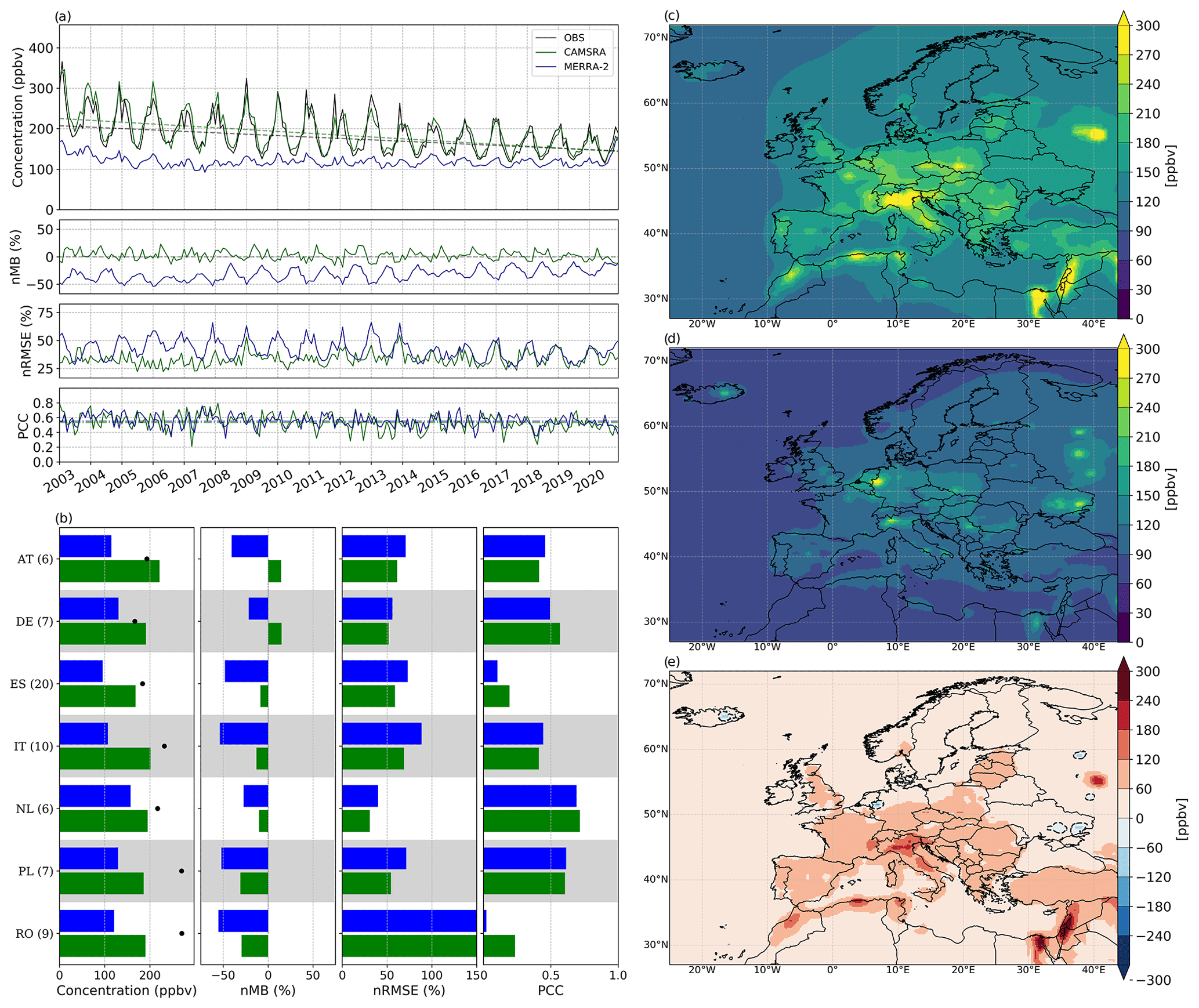
Figure 4Similar to Fig. 2 but for CO.
At monthly scale, the median [CO], nMB and nRMSE in CAMSRA partially capture the seasonality, showing a better performance in autumn (0 %) and summer (31 %) and a moderate springtime (+9 %) and wintertime (39 %) deterioration, respectively. As seen for O3, the PCC follows the opposite behaviour, with better performance in DJF (0.58) and a late springtime deterioration (0.46). In contrast to CAMSRA, MERRA-2 is unable to reproduce the seasonal variability of surface [CO], despite the nMB and nRMSE displaying significant variability throughout the different seasons. A surprisingly large increase in [CO] is found in MERRA-2 throughout 2020. It is unclear what stands behind such a significant increase, but this abrupt change affects mostly specific pollution hotspots in the European continent, including the Rhine-Rühr valley and the Paris and London metropolitan areas, as well as the Po River basin. This [CO] surge is also found in the raw version (i.e. non-regridded) of the reanalysis. The strong statistically significant decrease in CO observed across Europe over 2003–2020 (−3.47 ppbv yr−1) is moderately overestimated in CAMSRA (−4.56 ppbv yr−1), although less dramatically than in MERRA-2, where CO remains roughly constant over all of the study period, displaying a small negative trend (−0.44 ppbv yr−1). In Pinterits et al. (2021) the EEA reports a CO emission trend of −2.3 % yr−1 over 1990–2019, relatively close to the mixing ratio trends found in CAMSRA, −2.4 % yr−1, and the observations, −1.9 % yr−1. In 2020, MERRA-2 shows a very large increase in [CO] across most of Europe, in contrast to both CAMSRA and the observations. The overall PCC in MERRA-2 and CAMSRA is poor (0.22 and 0.28, respectively), although better PCC values (∼ 0.40) are found at monthly scale (0.53 and 0.55, respectively).
This CO underestimation typically spreads over the whole European continent, with strong differences across countries. As CO is not assimilated in MERRA-2 but simulated by the GEOS-5 modelling system, this underestimation likely comes from a poor representation of CO emissions and/or excessively large CO sinks. In both reanalyses, the best scores in terms of bias, PCC and nRMSE are found in Germany (DE) and to a lesser extent in the Netherlands (NL). Conversely, far poorer results are obtained in Poland (PL) and Romania (RO). Although different, the nMB and nRMSE in both reanalyses typically show comparable variations from one country to another. Both CAMSRA and MERRA-2 show CO hotspots over large urban areas and/or highly industrialized regions (e.g. Moscow, Po River basin). However, compared to CAMSRA, MERRA-2 highlights some additional hotspots, for instance on the Vatnajökull ice cap, located in Iceland, a region well known for its sub-glacial volcanoes (e.g. Grímsvötn) which experience frequent degassing. Another significant hotspot is found in the Donets Basin (eastern Ukraine), an important coal mining region. Two other CO hotspots can be seen south and north of Moscow, corresponding to the cities of Voronezh and Yaroslavl, respectively, but it is unlikely that CO levels comparable to those of Moscow are found in these intermediate-sized cities (Fig. 4c, d).
The reanalyses also differ in the locations where [CO] is higher across Europe (Po River basin in CAMSRA; Rhine-Rühr Valley in MERRA-2). CAMSRA highlights the highest CO mixing ratios in Europe in the Po River basin and displays moderate mixing ratio values in the Rhine-Rühr area, which suggests a longer CO lifetime in the former given that Pinterits et al. (2021) reports the highest CO emissions, over the whole period of 1990–2019, in Germany. Therefore, in sharp contrast to CAMSRA, MERRA-2 obviously fails to capture the chemistry processes of surface CO, with a likely underestimation of emission sources and/or too large CO sinks, thus being unable to reproduce the spatiotemporal variability of surface CO observed over Europe.
From Table B1 it immediately becomes apparent that the main difference between the urban and rural subsets, aside from the large variation in baseline mixing ratios, comes from CAMSRA largely underestimating the observed [CO] in urban cells, with the nMB (−46 %) nearly quadrupling when compared to the rural evaluation. For MERRA-2 the nMB also suffers from a deterioration (−64 %) but more limited due to an already large bias in the rural subset. For both CAMSRA and MERRA-2, the overall nRMSE (91 % and 105 %, respectively) and PCC (0.39 and 0.19, respectively) remain close to the rural values, with no significant variations. The seasonal behaviour of both reanalyses also remains unchanged, with MERRA-2 completely missing the amplitude of the seasonal cycle. This large amplitude is also the reason why CAMSRA loses its ability to reproduce the observed CO mixing ratio.
3.4 Sulfur dioxide (SO2)
When computed over the entire dataset (Table 4), the statistics of CAMSRA and MERRA-2 show very poor nRMSE and PCC (around 143 % and 0.33–0.35, respectively) but better performance in terms of bias for CAMSRA (+10 %) than for MERRA-2 (+40 %). On average, the overestimation of MERRA-2 is much higher in winter, meaning the amplitude of the SO2 seasonal cycle is strongly overestimated (Fig. A1).
At monthly scale (Fig. 5a), the median nMB in MERRA-2 severely deteriorates (+75 %) and increases throughout time, with the worst performance peaking in SON (+94 %) and a slight springtime improvement (+57 %). The median monthly scale nMB in CAMSRA tends to improve between late spring and early summer, reaching values close to 0 %, though it oscillates throughout the year, dropping to −12 % in winter and peaking at +11 % in autumn. Note that Ryu and Min (2021), though finding a larger [SO2] overestimation over South Korea, greater than the underestimation shown here for Europe, found a similar nMB seasonality, with nMB improving (∼ +2 ppbv) and worsening (∼ +6 ppbv) in warm and cold months, respectively. In MERRA-2 the median nMB oscillates roughly around +69 % (with a ±3 % range), though it suffers from an important increase (with significant intra-annual variability) from 2013 onwards due to a decrease in observed [SO2]. A similar increase is also observed in the nRMSE. The monthly scale nRMSE and PCC remain roughly constant (when averaged across all months) throughout all seasons, both in CAMSRA (around 70 % and 0.28, respectively) and in MERRA-2 (around 108 % and 0.31, respectively), though the latter displays much stronger seasonal variability. Note also the large difference between the monthly scale nRMSE (70 %–108 %) and the overall nRMSE (around 143 %). The statistically significant negative trend found in observed SO2 mixing ratios (−0.034 ppbv yr−1) is largely overestimated by CAMSRA (−0.078 ppbv yr−1) and well reproduced by MERRA-2 (−0.033 ppbv yr−1) (Fig. 5). In Pinterits et al. (2021) the EEA reports a SO2 anthropogenic emission trend of −3.2 % yr−1 over 1990–2019, falling between the mixing ratio trend found in CAMSRA, −6.2 % yr−1, and the one found in the observations, −2.7 % yr−1, and MERRA-2, −1.5 % yr−1.
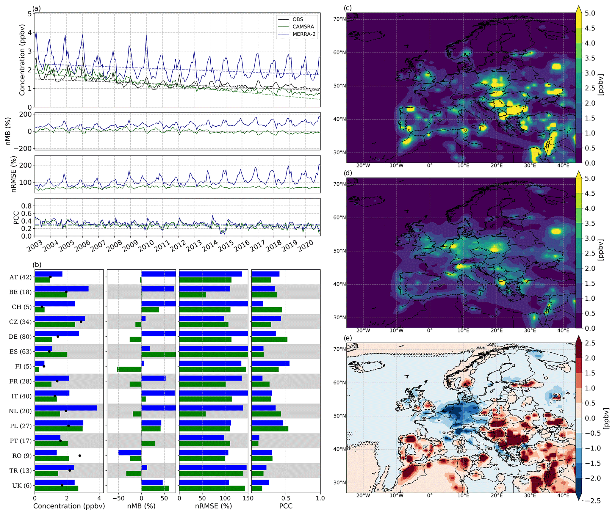
Figure 5Similar to Fig. 2 but for SO2.
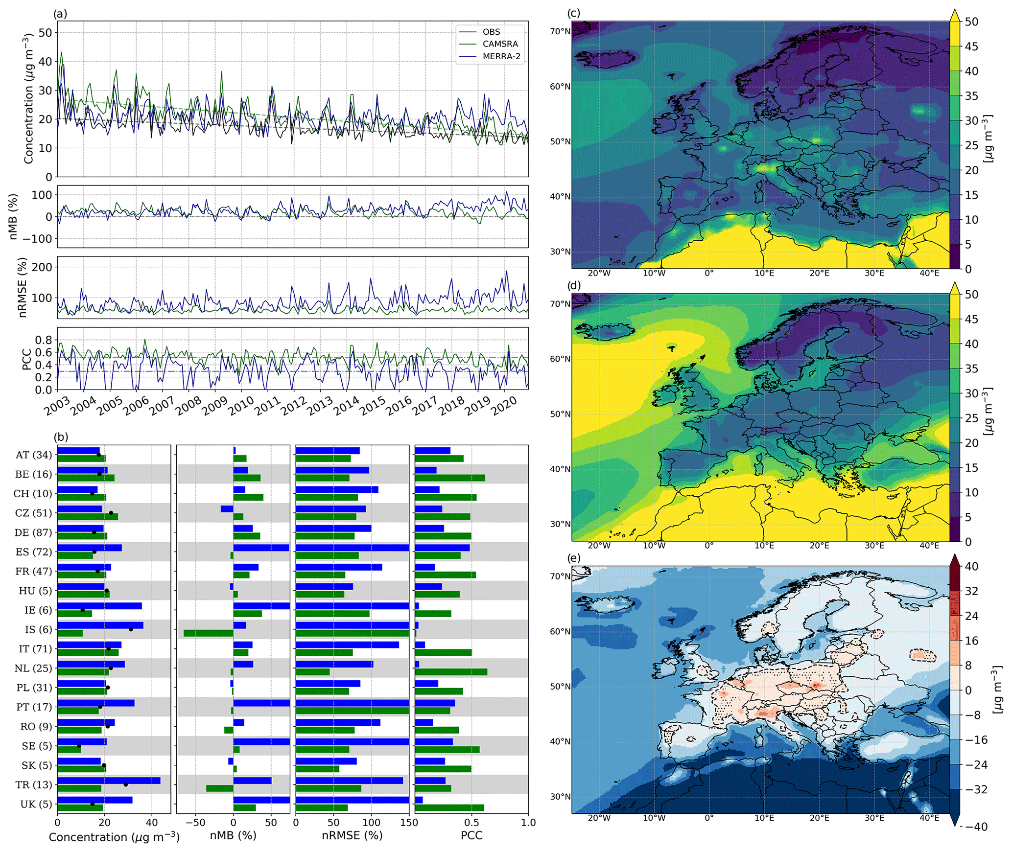
Figure 6Similar to Fig. 2 but for PM10.
The country-level evaluation for SO2 shows very heterogeneous results across countries, differing substantially from the observed behaviour in previously examined reactive gases. The nMB presents a wide range of variation, with certain countries showing very reduced biases for at least one of the reanalyses (e.g. Portugal, Czech Republic, Austria, Belgium) and others presenting biases well over ±50 % (e.g. the United Kingdom, France, Romania, Switzerland). Both the nRMSE and PCC display a poor performance, ranging roughly within 100 %–150 % and 0.10–0.50, respectively (Fig. 5b). Upon a first examination of the SO2 spatial distribution, it may appear as if the mixing ratio values in the time series should be larger for CAMSRA, though this is actually misleading, as the evaluation is performed only in cells with available observations. Therefore, regions with a higher station density contribute more towards the final mixing ratio value. From Fig. 5e it can be immediately seen that MERRA-2 presents higher SO2 mixing ratios in several countries which have an overall larger number of stations (e.g. Germany, the Netherlands, France, Italy).
In both reanalyses, the heterogeneous distribution of [SO2] is consistent with the location of highly industrialized areas (e.g. Po River basin, Rhine-Rühr Valley) and coal mining regions (e.g. Silesia, Donets Basin, Balkans). To a minor extent, there are also significant SO2 mixing ratios in dense urban areas and along shipping lanes. Surprisingly, the aforementioned CO hotspot found in MERRA-2 over the Icelandic Vatnajökull ice cap does not come with an associated SO2 hotspot, which contrasts with the fact that SO2 emissions represent a large fraction of volcanic gases. The reanalyses show sharp differences in the regions where the highest mixing ratios of SO2 are present, with CAMSRA favouring coal mining regions and dense urban areas and MERRA-2 showing a more balanced distribution between them (Fig. 5c, d, e). Overall, both reanalysis products present distinct although substantial deficiencies in their representation of SO2 mixing ratios, with the increasing overestimation of MERRA-2 probably being the most critical issue. Anthropogenic SO2 emissions in MERRA-2 are obtained from AeroCom Phase II (Diehl et al., 2012) and EDGAR v4.2 (Janssens-Maenhout et al., 2011; Janssens-Maenhout, 2011) inventories, with emissions fixed to those of the last year available in each inventory (Randles et al., 2017). Thus, the progressive deterioration of the bias in MERRA-2, particularly notorious from 2013 onwards, likely arises due to an emission overestimation which propagates throughout the time period where no updated SO2 emissions are available.
When considering urban background stations, both CAMSRA and MERRA-2 shift towards a moderate negative nMB (−29 % and −26 %, respectively), far from the positive bias found in the rural subset. Overall, both the nRMSE (247 % and 251 %, respectively) and PCC (0.18 and 0.08, respectively) are extremely poor (see Table B1). The mixing ratio in CAMSRA presents significant intra-annual variability and thus fails to correctly reproduce the observed seasonal behaviour. MERRA-2 shows a much better ability to capture the seasonality of [SO2], though it still suffers from the increasing overestimation previously highlighted for rural background stations.
3.5 Coarse particulate matter (PM10)
Overall, CAMSRA and MERRA-2 reanalyses represent surface PM10 concentrations over Europe (Table 4) moderately well, with a limited positive nMB (+14 %) for CAMSRA and moderate bias for MERRA-2 (+29 %) but poor nRMSE (81 % and 129 %, respectively) and PCC (0.45 and 0.22, respectively).
At monthly scale, the median nMB in CAMSRA presents a strong seasonality, with an important deterioration during spring (+36 %) and better performance in DJF (+5 %), while the nRMSE and PCC show a strong and complex intra-annual variability without a clear seasonal pattern (remaining in the range of 53 %–65 % and 0.48–0.54, respectively). In comparison, nRMSE and PCC in MERRA-2 follow a clear seasonal behaviour, with strongly deteriorated results during winter (105 % and 0.11, respectively) but better summertime performance (71 % and 0.41, respectively). Surprisingly, the median nMB in MERRA-2 also peaks in JJA (+38 %), with a small bias reduction in SON and a wintertime low (+24 %). Ryu and Min (2021) found a slightly positive PM10 bias for CAMSRA in South Korea over 2003–2018, while for MERRA-2 their findings suggest a clear underestimation that worsens significantly in winter, the former being in good agreement with our results over Europe. The statistically significant negative trend present in the observations (−0.36 ) is strongly overestimated by CAMSRA (−0.70 ) and severely underestimated by MERRA-2 (−0.02 ), with the latter not being statistically significant (at a 99 % confidence level). In Pinterits et al. (2021) the EEA reports a PM10 emission trend of −1.7 % yr−1 over 2000–2019, far from the concentration trend of CAMSRA, −3.3 % yr−1, but closer to the one found in the observations, −2.1 % yr−1.
At a country level, CAMSRA tends to outperform MERRA-2 in most countries, with lower nRMSE (50 %–100 % and 75 %–150 %, respectively) and higher PCC values (0.3–0.6 against 0.1–0.4, respectively). The nMB presents a wide range of variation in both reanalyses, with certain countries showing virtually no bias for MERRA-2 (e.g. Austria), for CAMSRA (e.g. Spain, the Netherlands, Portugal) or for both reanalyses (e.g. Poland, Hungary, Slovakia). Other countries present biases well over ±25 % (e.g. Turkey, Germany, Ireland, the United Kingdom). Though MERRA-2 presents lower nMB values than CAMSRA in several countries (e.g. Iceland, Germany, Czech Republic, Belgium), both the nRMSE and PCC point towards a greater performance by CAMSRA in all cases (Fig. 6b).
Again, despite its finer resolution, MERRA-2 displays a more homogeneous concentration over land in which the multiple PM10 hotspots found in CAMSRA – in industrialized regions (e.g. Po River basin, Silesia) and in certain urban areas (e.g. Paris, Moscow, Madrid) – are missing. In addition, it also shows much higher PM10 concentrations over the open seas and North Africa, where sea salt and dust sources are predominant. It thus seems that Eq. (2a) severely overestimates the surface concentrations of PM10, as shown in Fig. 6d), with MERRA-2 displaying differences of more than a 100 µg m−3, particularly over desert areas. This overestimation is likely related to sea salt and dust concentrations in the model being overestimated, as shown in the Supplement. Overall, CAMSRA unambiguously outperforms MERRA-2 in capturing the spatiotemporal variability of PM10 surface concentrations over Europe.
As shown in Table B1, both CAMSRA and MERRA-2 present limited negative nMB (−20 and −8 %, respectively) for the urban subset, which contrasts with the positive bias found for rural stations. For both reanalyses, the overall nRMSE (85 % and 112 %, respectively) and PCC (0.36 and 0.19, respectively) remain close to their rural counterparts, with no significant variations. The observed PM10 concentration is characterized by strong intra-annual variability, though certain seasonality is still present.
3.6 Fine particulate matter (PM2.5)
MERRA-2 reproduces surface PM2.5 concentrations over Europe (Table 4) moderately well, with a low negative nMB (−9 %) but poor nRMSE and PCC (98 % and 0.29, respectively), while CAMSRA presents an overall worst nMB (+14 %), similar nRMSE (96 %) and slightly better but still moderate PCC (0.43).
The median monthly scale nMB in CAMSRA presents a clear seasonal pattern, with the bias heavily deteriorating in MAM and JJA (+41 %) but virtually vanishing in DJF (+1 %). MERRA-2 also shows a clear seasonality, with the largest over- and underestimations occurring during summer (+21 %) and winter (−17 %), respectively. Interestingly, the MERRA-2 and CAMSRA nMB time series, while initially displaying an absolute difference of ∼ 50 %, converge from 2017 onwards. Similarly to the behaviour observed for PM10, the median nRMSE and PCC in CAMSRA show a strong intra-annual variability without a clear seasonal pattern (remaining in the range of 61 %–74 % and 0.48–0.53, respectively). As for MERRA-2, both the nRMSE and the PCC present significant seasonal variability, with better performance in summer (50 % and 0.58, respectively) and a sharp wintertime deterioration (74 % and 0.36, respectively). Similar results are reported by Provençal et al. (2017a) when evaluating MERRA-1 over Europe, with an overall limited negative bias and a deterioration in winter. Note also that Navinya et al. (2020) evaluated PM2.5 in MERRA-2 against 20 background stations in India, finding a moderate negative nMB (−34 %; −27 µg m−3) and a larger wintertime underestimation, in agreement with our results over Europe. The negative trend present in the observations (−0.10 ) has been found to not be statistically significant, though it is strongly overestimated by CAMSRA (−0.23 ) and completely missed by MERRA-2. As a consequence, though the nMB time series of CAMSRA and MERRA-2 differ by more than 30 % in 2003, they end up converging progressively along the period 2003–2020. In Pinterits et al. (2021) the EEA reports a PM2.5 emission trend of −1.9 % yr−1 over 2000–2019 which, while not directly comparable to a concentration trend as previously mentioned, is close to the trend found in CAMSRA, −1.7 % yr−1, but far from the one found in the observations, −0.9 % yr−1.
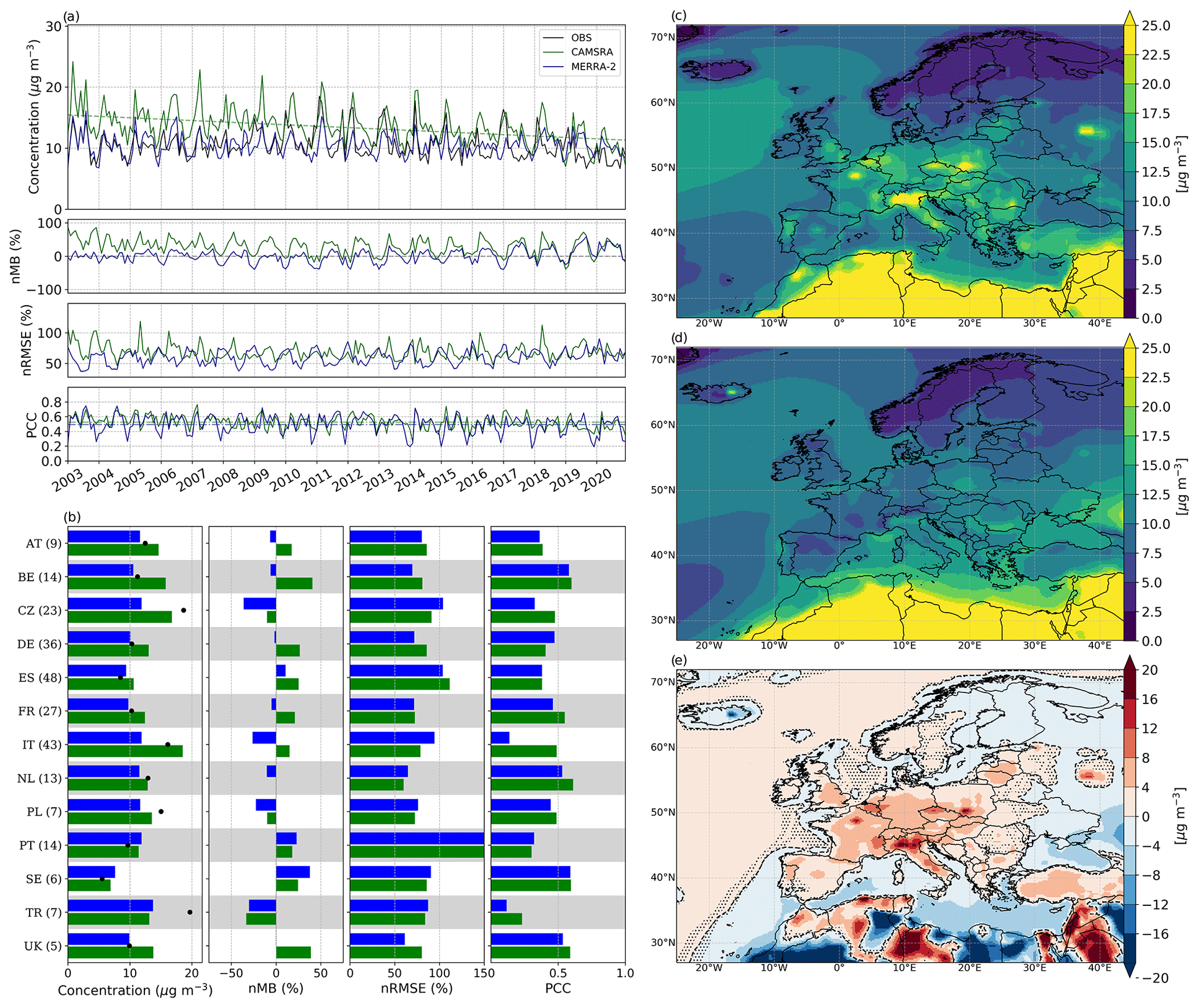
Figure 7Similar to Fig. 2 but for PM2.5.
At a country level (Fig. 7b), the differences in PM2.5 between CAMSRA and MERRA-2 are less pronounced than for PM10, especially for the PCC (with most values in the range 0.3–0.6), and to a lesser extent for the nRMSE (with most values in the range of 60 %–100 %). The nMB presents a similar behaviour to the one observed for PM10, with certain countries showing virtually no bias for CAMSRA (e.g. the Netherlands) or MERRA-2 (e.g. the United Kingdom, France, Germany, Belgium) and other countries presenting important negative/positive biases (e.g. Turkey, Sweden).
The spatial variability of the PM2.5 concentration remains close to the one obtained for PM10 in all regions and in both reanalyses, except over the open seas, where MERRA-2 no longer shows exceedingly large sea salt levels (which thus prevail mostly in the coarse mode). The surface pollution hotspots present in Fig. 7 are essentially the same ones that appear in Fig. 6, though a notable exception is observed in MERRA-2 over Iceland. A large PM2.5 concentration peak, also visible for PM10, can be spotted in Iceland's time series during 2010, surpassing 100 µg m−3, likely due to the Eyjafjallajökull volcanic eruption, which emitted very large amounts of volcanic ash (Thorsteinsson et al., 2012).
As for urban background stations, CAMSRA presents an overall small negative nMB (−13 %), while MERRA-2 displays a larger but limited negative bias (−30 %). In terms of nRMSE and PCC, both CAMSRA and MERRA-2 perform rather poorly, with large errors (86 % and 96 %, respectively) and low correlations (0.41 and 0.24, respectively). Similarly to PM10, the observed PM2.5 concentration shows strong intra-annual variability, though a seasonal pattern is also visible.
In this work we have performed a long-term (2003–2020) multi-pollutant evaluation of CAMSRA and MERRA-2 global atmospheric composition reanalyses against in situ surface measurements over the European continent. In contrast to past evaluation studies, we have included a more extended set of rural background stations, from several hundred to a few thousand depending on the pollutant considered (Table 3), quality assured using GHOST metadata and gridded in order to limit, to some extent, representativeness issues. Results obtained against urban background stations have also been briefly discussed.
As a summary, CAMSRA unambiguously outperforms MERRA-2 in representing surface pollutant concentrations across Europe. Differences are particularly clear for O3 and CO but also persist for PM10 and PM2.5. CAMSRA clearly achieves the best results for O3, while statistics for the other pollutants show more mixed results: substantial overestimation, moderate error but reasonable correlation for NO2, low biases, poor error and moderate correlation for PM10 and PM2.5, and low biases but poor errors and correlations for CO and SO2. With MERRA-2 being designed mainly for research on aerosols, the reanalysis indeed provides statistics on PM10 and PM2.5 in line with CAMSRA, but the latter still gives slightly better results over Europe, especially for PM10, with overall lower biases and a better characterization of its spatial variability.
Compared to CAMSRA, MERRA-2 benefits from a slightly finer spatial resolution but assimilates a much less diversified set of satellite products. However, recent evaluations of CAMSRA have noticed that this assimilation only partially improves the representation of pollutant concentrations at the surface, despite a clear improvement being found in the entire troposphere. Although at least partly due to the still coarse spatial resolution of CAMSRA, a large if not dominant part of the model-versus-observation differences found here at the surface are likely explained by errors in emissions and/or sinks. Therefore these global reanalysis datasets need to be carefully bias corrected with surface observations in order to be used in long-term air pollution and impact studies.
The surface pollution evaluation carried out in this work can serve as a milestone for future air quality and other pollution-related studies. In that regard, further advancements in the field could focus on developing new statistical approaches to merge surface observations with reanalysis data. As global atmospheric composition reanalyses do not assimilate data at the surface, ground-level measurements can be employed, through different statistical methods, to bias correct and to improve raw model output statistics, thus leading to more robust reanalysis products. This improved characterization of the spatiotemporal variability of surface air pollution would open the door to improved health impact and air quality assessments, while also helping design and implement more effective air pollution reduction policies.
Eventually, if reanalyses are to be used in long-term health impact studies, consistent statistical approaches to combine observational data with reanalysis data need to be further developed.
Seasonal-scale statistics (Tables A1–A6) and mean monthly profiles (Figs. A1–A2) are shown here for rural and urban background stations.
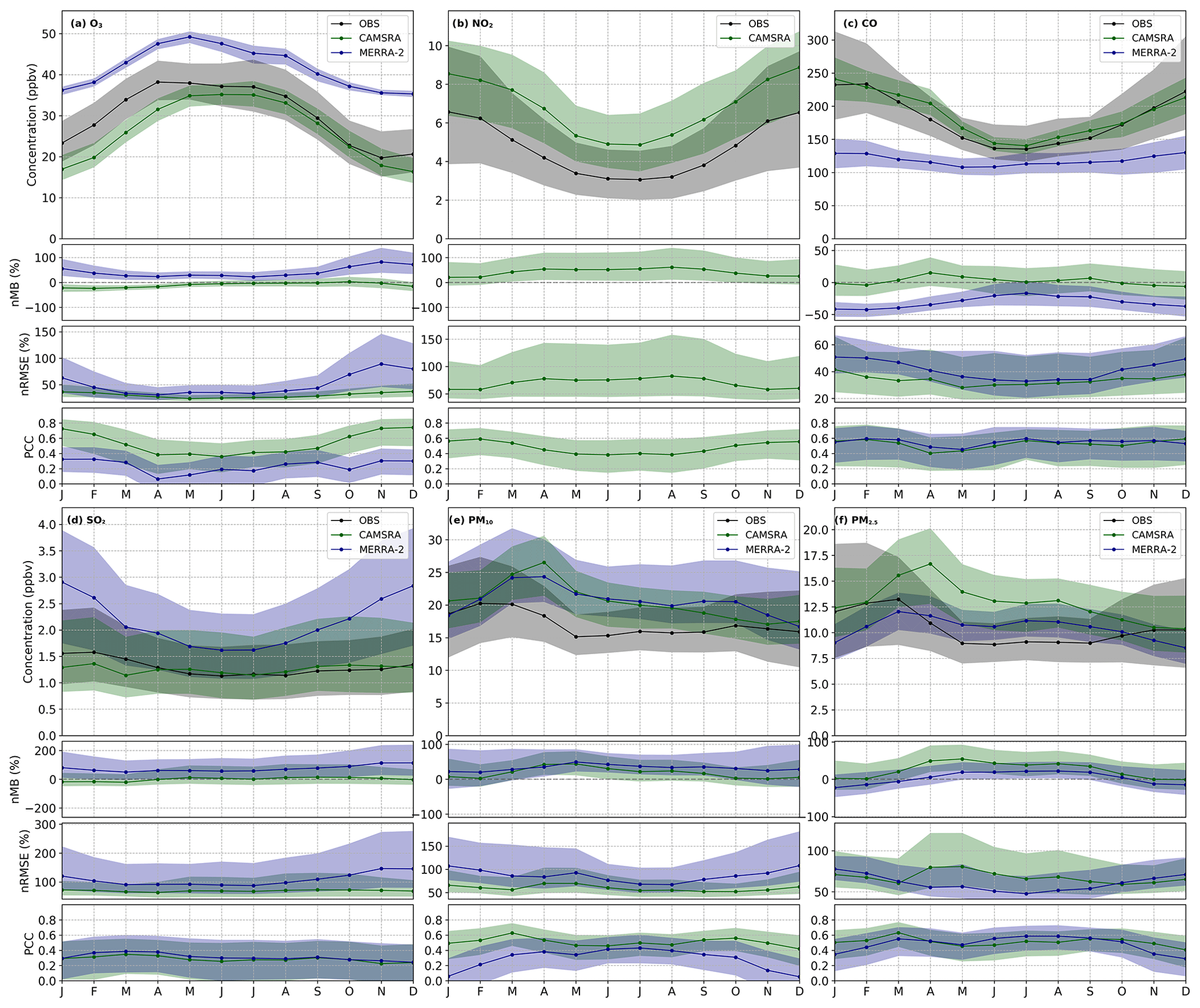
Figure A1Seasonal variability of [O3], [NO2], [CO], [SO2], [PM10] and [PM2.5] over the period 2003–2020 across Europe evaluated against rural background stations. For each pollutant the panels show, from top to bottom, concentration, nMB, nRMSE and PCC. The black, green and blue lines represent observations, CAMSRA and MERRA-2, respectively. Shaded contours indicate the 25th (bottom) and 75th (top) percentiles. All monthly values are weighted by the number of points, N, over the period 2003–2020.
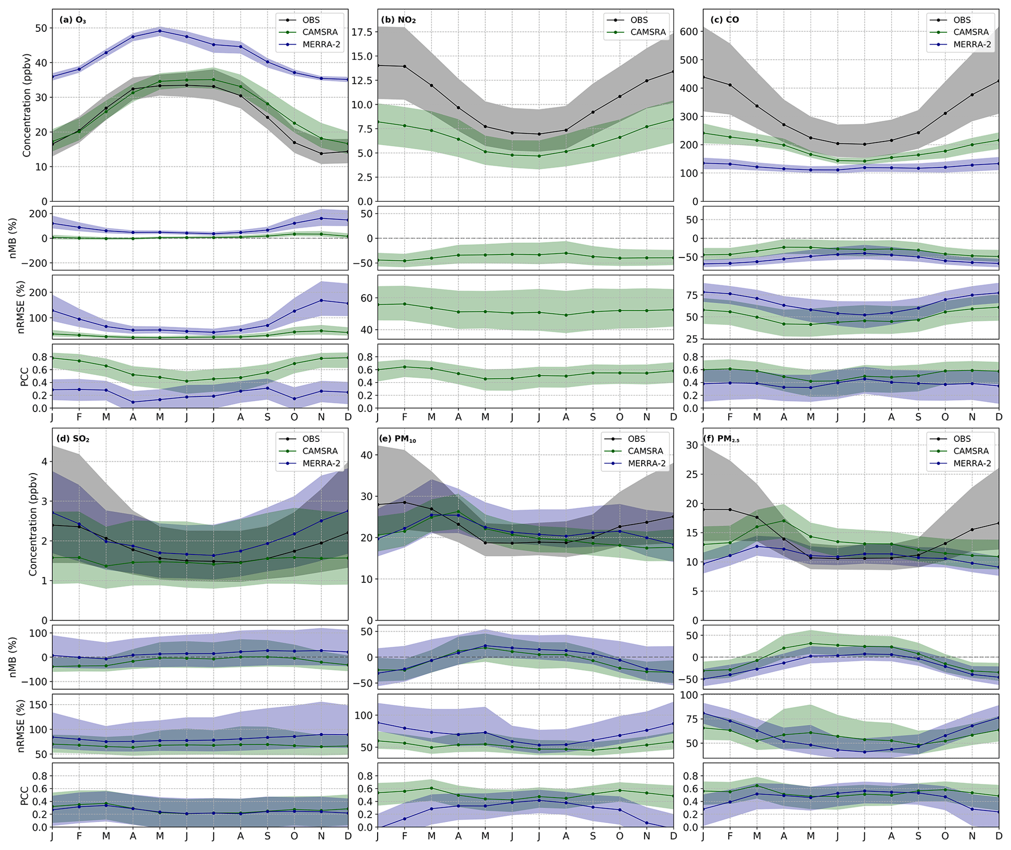
Table A1O3 seasonal statistics over the period 2003–2020 across Europe for CAMSRA (subscript C) and MERRA-2 (subscript M). Statistics are shown both on a daily scale (d; over all cells and days in the period 2003–2020) and on a monthly scale (m; weight averaged over all median monthly values). Reactive gas concentrations are expressed in ppbv and normalized statistics in %.
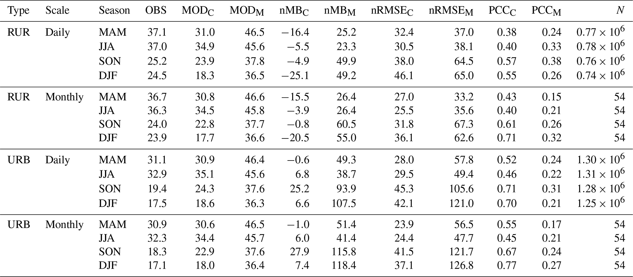
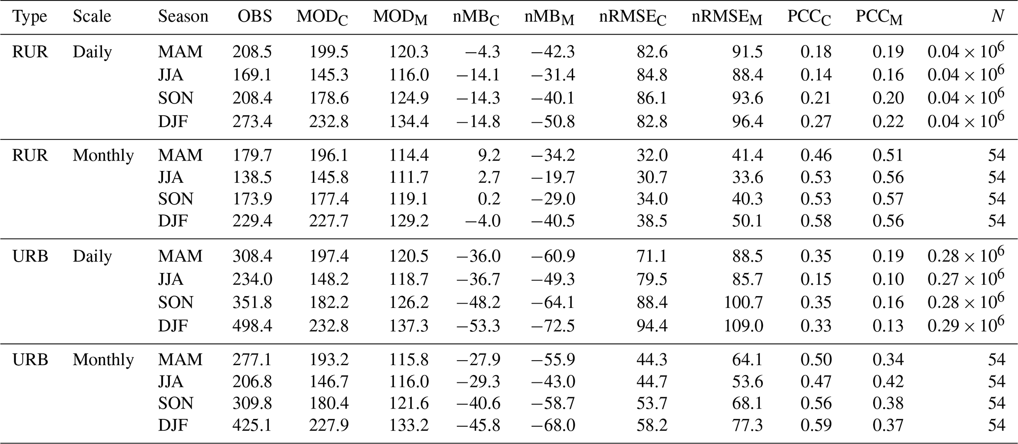
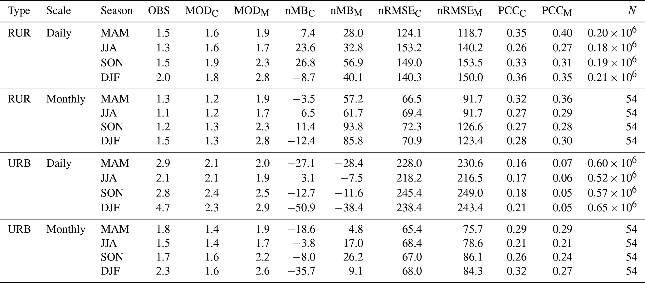
Table A5The same as Table A1 but for PM10. Aerosol concentrations are expressed in µg m−3.
Given that our monthly time series does not contain tied or missing values, the seasonal Mann–Kendall statistic, S′, and its variance, Var[S′], can be obtained as follows:
where n and m are the number of years and seasons (i.e. here monthly values), respectively; Sg is the Mann–Kendall statistic for each gth season; Rg and Rh are Spearman's correlation coefficients for seasons g and h, respectively; and sgn(x) is the sign function. Seasonal Theil–Sen slopes (i.e. annual trends) are then derived from S′ (Hussain and Mahmud, 2019; McCuen, 1995; Hirsch and Slack, 1984). The confidence intervals, derived from Var[S′], are computed accounting for seasonality but not for autocorrelation, mainly due to the detection of a potential bug in the function correlated_multivariate_test from the Python library pyMannKendall (Hussain and Mahmud, 2019), which at the date of this work's submission remained unresolved.
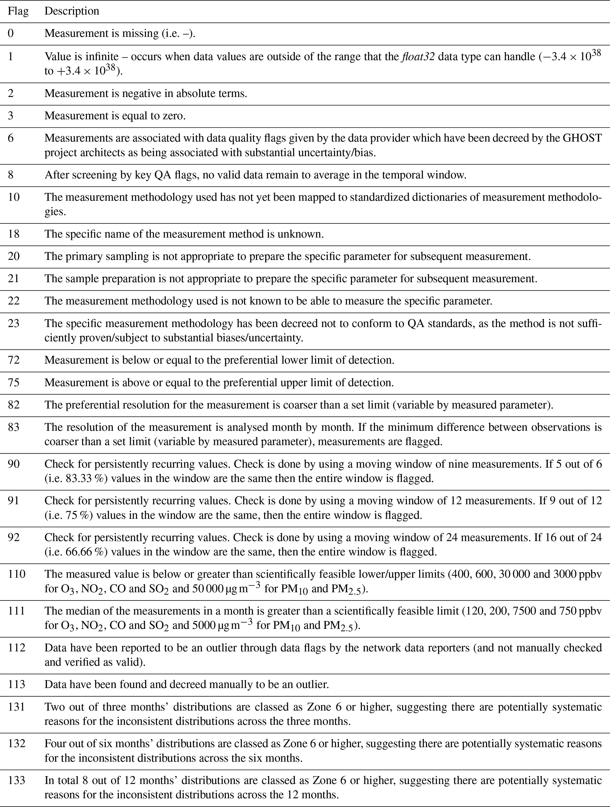
Using the metadata available in GHOST, a quality assurance screening is applied by removing all air quality observations associated with a set of flags detailed in Table D1. In addition, we detected a few very low CO concentrations in specific regions during specific time periods, which we suspect originate from errors in units when the member state reported its observations to the EEA. Therefore, as a precautionary measure, all CO hourly observations below 1 ppbv were discarded in this study.
Table D1Description of the GHOST quality assurance flags used on the EEA air quality observational dataset.
The observational data, obtained from the EEA AirBase and AQ e-Reporting air quality datasets, and reanalysis data, obtained from CAMSRA and MERRA-2, used in this study are publicly available. CAMSRA, MERRA-2 and EEA observational data can be obtained respectively from the Atmosphere Data Store (ADS; https://atmosphere.copernicus.eu/data, CAMS, 2023), the NASA Goddard Earth Sciences Data and Information Services Center (GES DISC; https://disc.gsfc.nasa.gov/datasets?project=MERRA-2, NASA, 2023), and the European Environment Agency websites for AQ e-Reporting (https://www.eea.europa.eu/data-and-maps/data/aqereporting-9, EEA, 2023a) and AirBase (https://www.eea.europa.eu/data-and-maps/data/airbase-the-european-air-quality-database-8, EEA, 2014).
The supplement related to this article is available online at: https://doi.org/10.5194/gmd-16-2689-2023-supplement.
AL carried out the analysis. AL and HP contributed to the conception and design of the study. DB was responsible for the acquisition and preprocessing of the air quality data through the GHOST project. AL, HP, ZC, RFMT, HA, CPGP, OJ, AS and JB contributed to the interpretation of the results. AL and HP were responsible for writing the manuscript, with reviews from CPGP and AS.
The contact author has declared that none of the authors has any competing interests.
Publisher’s note: Copernicus Publications remains neutral with regard to jurisdictional claims in published maps and institutional affiliations.
We acknowledge Red Temática ACTRIS España (CGL2017-90884-REDT), PRACE and RES for awarding us access to the MareNostrum Supercomputer in the Barcelona Supercomputing Center, and H2020 ACTRIS IMP(#871115). Last but not least, we gratefully acknowledge the outstanding work done by the Python development teams behind some specific libraries, including numpy, scipy, pandas, xarray, matplotlib and cartopy.
This research has received funding from the European Research Council (ERC), in the frame of the EARLY-ADAPT project (https://early-adapt.eu/, last access: 15 December 2022), under the European Union’s Horizon 2020 research and innovation programme (grant no. 865564), as well as the MITIGATE project (project no. PID2020-116324RA I00/AEI/10.13039/501100011033) from the Agencia Estatal de Investigación (AEI). We also acknowledge support by the AXA Research Fund.
This paper was edited by Fiona O'Connor and reviewed by three anonymous referees.
Aldabe, J., Elustondo, D., Santamaría, C., Lasheras, E., Pandolfi, M., Alastuey, A., Querol, X., and Santamaría, J. M.: Chemical characterisation and source apportionment of PM2.5 and PM10 at rural, urban and traffic sites in Navarra (North of Spain), Atmos. Res., 102, 191–205, https://doi.org/10.1016/j.atmosres.2011.07.003, 2011. a
Ali, M. A., Bilal, M., Wang, Y., Nichol, J. E., Mhawish, A., Qiu, Z., de Leeuw, G., Zhang, Y., Zhan, Y., Liao, K., Almazroui, M., Dambul, R., Shahid, S., and Islam, M. N.: Accuracy assessment of CAMS and MERRA-2 reanalysis PM2.5 and PM10 concentrations over China, Atmos. Environ., 288, 119297, https://doi.org/10.1016/j.atmosenv.2022.119297, 2022. a, b
Barré, J., Petetin, H., Colette, A., Guevara, M., Peuch, V.-H., Rouil, L., Engelen, R., Inness, A., Flemming, J., Pérez García-Pando, C., Bowdalo, D., Meleux, F., Geels, C., Christensen, J. H., Gauss, M., Benedictow, A., Tsyro, S., Friese, E., Struzewska, J., Kaminski, J. W., Douros, J., Timmermans, R., Robertson, L., Adani, M., Jorba, O., Joly, M., and Kouznetsov, R.: Estimating lockdown-induced European NO2 changes using satellite and surface observations and air quality models, Atmos. Chem. Phys., 21, 7373–7394, https://doi.org/10.5194/acp-21-7373-2021, 2021. a
Bauwens, M., Compernolle, S., Stavrakou, T., Müller, J. F., van Gent, J., Eskes, H., Levelt, P. F., van der A, R., Veefkind, J. P., Vlietinck, J., Yu, H., and Zehner, C.: Impact of Coronavirus Outbreak on NO2 Pollution Assessed Using TROPOMI and OMI Observations, Geophys. Res. Lett., 47, e2020GL087978, https://doi.org/10.1029/2020GL087978, 2020. a
Bosilovich, M., Akella, S., Coy, L., Cullather, R., Draper, C., Gelaro, R., Kovach, R., Liu, Q., Molod, A., Norris, P., Wargan, K., Chao, W., Reichle, R., Takacs, L., Vikhliaev, Y., Bloom, S., Collow, A., Firth, S., Labow, G., Partyka, G., Pawson, S., Reale, O., Schubert, S. D., and Suarez, M.: MERRA-2: Initial Evaluation of the Climate, NASA Technical Report Series on Global Modeling and Data Assimilation, 43, 139 pp., https://gmao.gsfc.nasa.gov/pubs/docs/Bosilovich803.pdf (last access: 15 December 2022), 2015. a
Buchard, V., da Silva, A. M., Randles, C. A., Colarco, P., Ferrare, R., Hair, J., Hostetler, C., Tackett, J., and Winker, D.: Evaluation of the surface PM2.5 in Version 1 of the NASA MERRA Aerosol Reanalysis over the United States, Atmos. Environ., 125, 100–111, https://doi.org/10.1016/j.atmosenv.2015.11.004, 2016. a, b
Buchard, V., Randles, C. A., da Silva, A. M., Darmenov, A., Colarco, P. R., Govindaraju, R., Ferrare, R., Hair, J., Beyersdorf, A. J., Ziemba, L. D., and Yu, H.: The MERRA-2 aerosol reanalysis, 1980 onward. Part II: Evaluation and case studies, J. Climate, 30, 6851–6872, https://doi.org/10.1175/JCLI-D-16-0613.1, 2017a. a
Buchard, V., Randles, C. A., da Silva, A. M., Darmenov, A., Colarco, P. R., Govindaraju, R., Ferrare, R., Hair, J., Beyersdorf, A. J., Ziemba, L. D., and Yu, H.: The MERRA-2 aerosol reanalysis, 1980 onward. Part II: Evaluation and case studies, J. Climate, 30, 6851–6872, https://doi.org/10.1175/JCLI-D-16-0613.1, 2017b. a
Chin, M., Ginoux, P., Kinne, S., Torres, O., Holben, B. N., Duncan, B. N., Martin, R. V., Logan, J. A., Higurashi, A., and Nakajima, T.: Tropospheric aerosol optical thickness from the GOCART model and comparisons with satellite and sun photometer measurements, J. Atmos. Sci., 59, 461–483, https://doi.org/10.1175/1520-0469(2002)059<0461:taotft>2.0.co;2, 2002. a, b
Colarco, P., Da Silva, A., Chin, M., and Diehl, T.: Online simulations of global aerosol distributions in the NASA GEOS-4 model and comparisons to satellite and ground-based aerosol optical depth, J. Geophys. Res.-Atmos., 115, D14207, https://doi.org/10.1029/2009JD012820, 2010. a, b
Copernicus Atmosphere Monitoring Service (CAMS): Atmosphere Data Store, Copernicus Atmosphere Monitoring Service (CAMS) [data set], https://atmosphere.copernicus.eu/data (last access: 2 January 2023), 2023. a
Cuesta, J., Eremenko, M., Liu, X., Dufour, G., Cai, Z., Höpfner, M., von Clarmann, T., Sellitto, P., Foret, G., Gaubert, B., Beekmann, M., Orphal, J., Chance, K., Spurr, R., and Flaud, J.-M.: Satellite observation of lowermost tropospheric ozone by multispectral synergism of IASI thermal infrared and GOME-2 ultraviolet measurements over Europe, Atmos. Chem. Phys., 13, 9675–9693, https://doi.org/10.5194/acp-13-9675-2013, 2013. a
Darmenov, A. and da Silva, A.: The Quick Fire Emissions Dataset (QFED) – Documentation of versions 2.1, 2.2 and 2.4., NASA Technical Report Series on Global Modeling and Data Assimilation, 38, https://ntrs.nasa.gov/citations/20180005253 (last access: 15 December 2022), 2015. a
Dee, D. and Uppala, S.: Variational bias correction in ERA-Interim, 26, https://www.ecmwf.int/en/elibrary/74146-variational-bias-correction-era-interim (last access: 27 December 2022), 2008. a
Diehl, T., Heil, A., Chin, M., Pan, X., Streets, D., Schultz, M., and Kinne, S.: Anthropogenic, biomass burning, and volcanic emissions of black carbon, organic carbon, and SO2 from 1980 to 2010 for hindcast model experiments, Atmos. Chem. Phys. Discuss., 12, 24895–24954, https://doi.org/10.5194/acpd-12-24895-2012, 2012. a, b, c, d, e
Duncan, B. N., Martin, R. V., Staudt, A. C., Yevich, R., and Logan, J. A.: Interannual and seasonal variability of biomass burning emissions constrained by satellite observations, J. Geophys. Res.-Atmos., 108, 4040, https://doi.org/10.1029/2002jd002378, 2003. a
European Environment Agency (EEA): AirBase – The European air quality database, EEA [data set], https://www.eea.europa.eu/data-and-maps/data/airbase-the-european-air-quality-database-8 (last access: 2 January 2023), 2014. a, b
European Environment Agency (EEA): Air Quality e-Reporting (AQ e-Reporting), EEA [data set], https://www.eea.europa.eu/data-and-maps/data/aqereporting-8 (last access: 2 January 2023), 2018. a
European Environment Agency (EEA): Air Quality e-Reporting (AQ e-Reporting), European Environment Agency [data set], https://www.eea.europa.eu/data-and-maps/data/aqereporting-9 (last access: 2 January 2023), 2023. a
Flemming, J., Huijnen, V., Arteta, J., Bechtold, P., Beljaars, A., Blechschmidt, A.-M., Diamantakis, M., Engelen, R. J., Gaudel, A., Inness, A., Jones, L., Josse, B., Katragkou, E., Marecal, V., Peuch, V.-H., Richter, A., Schultz, M. G., Stein, O., and Tsikerdekis, A.: Tropospheric chemistry in the Integrated Forecasting System of ECMWF, Geosci. Model Dev., 8, 975–1003, https://doi.org/10.5194/gmd-8-975-2015, 2015. a, b
Gelaro, R., McCarty, W., Suárez, M. J., Todling, R., Molod, A., Takacs, L., Randles, C. A., Darmenov, A., Bosilovich, M. G., Reichle, R., Wargan, K., Coy, L., Cullather, R., Draper, C., Akella, S., Buchard, V., Conaty, A., da Silva, A. M., Gu, W., Kim, G. K., Koster, R., Lucchesi, R., Merkova, D., Nielsen, J. E., Partyka, G., Pawson, S., Putman, W., Rienecker, M., Schubert, S. D., Sienkiewicz, M., and Zhao, B.: The modern-era retrospective analysis for research and applications, version 2 (MERRA-2), J. Climate, 30, 5419–5454, https://doi.org/10.1175/JCLI-D-16-0758.1, 2017. a, b
Granier, C., Bessagnet, B., Bond, T., D'Angiola, A., van der Gon, H. D., Frost, G. J., Heil, A., Kaiser, J. W., Kinne, S., Klimont, Z., Kloster, S., Lamarque, J. F., Liousse, C., Masui, T., Meleux, F., Mieville, A., Ohara, T., Raut, J. C., Riahi, K., Schultz, M. G., Smith, S. J., Thompson, A., van Aardenne, J., van der Werf, G. R., and van Vuuren, D. P.: Evolution of anthropogenic and biomass burning emissions of air pollutants at global and regional scales during the 1980–2010 period, Climatic Change, 109, 163–190, https://doi.org/10.1007/S10584-011-0154-1, 2011. a, b, c
Guenther, A., Nicholas, C., Fall, R., Klinger, L., Mckay, W. A., and Scholes, B.: A global model of natural volatile organic compound emissions s Raja the balance Triangle changes in the atmospheric accumulation rates of greenhouse Triangle Several inventories of natural and Exposure Assessment global scales have been two classes Fores, J. Geophys. Res., 100, 8873–8892, 1995. a
Hersbach, H., Bell, B., Berrisford, P., Hirahara, S., Horányi, A., Muñoz-Sabater, J., Nicolas, J., Peubey, C., Radu, R., Schepers, D., Simmons, A., Soci, C., Abdalla, S., Abellan, X., Balsamo, G., Bechtold, P., Biavati, G., Bidlot, J., Bonavita, M., De Chiara, G., Dahlgren, P., Dee, D., Diamantakis, M., Dragani, R., Flemming, J., Forbes, R., Fuentes, M., Geer, A., Haimberger, L., Healy, S., Hogan, R. J., Hólm, E., Janisková, M., Keeley, S., Laloyaux, P., Lopez, P., Lupu, C., Radnoti, G., de Rosnay, P., Rozum, I., Vamborg, F., Villaume, S., and Thépaut, J. N.: The ERA5 global reanalysis, Q. J. Roy. Meteor. Soc., 146, 1999–2049, https://doi.org/10.1002/qj.3803, 2020. a, b
Hirsch, R. M. and Slack, J. R.: A Nonparametric Trend Test for Seasonal Data With Serial Dependenc, Water Resour. Res., 20, 727–732, 1984. a
Huijnen, V., Miyazaki, K., Flemming, J., Inness, A., Sekiya, T., and Schultz, M. G.: An intercomparison of tropospheric ozone reanalysis products from CAMS, CAMS interim, TCR-1, and TCR-2, Geosci. Model Dev., 13, 1513–1544, https://doi.org/10.5194/gmd-13-1513-2020, 2020. a, b, c
Hussain, M. and Mahmud, I.: pyMannKendall: a python package for non parametric Mann Kendall family of trend tests., Journal of Open Source Software, 4, 1556, https://doi.org/10.21105/joss.01556, 2019. a, b
Inness, A., Ades, M., Agustí-Panareda, A., Barré, J., Benedictow, A., Blechschmidt, A.-M., Dominguez, J. J., Engelen, R., Eskes, H., Flemming, J., Huijnen, V., Jones, L., Kipling, Z., Massart, S., Parrington, M., Peuch, V.-H., Razinger, M., Remy, S., Schulz, M., and Suttie, M.: The CAMS reanalysis of atmospheric composition, Atmos. Chem. Phys., 19, 3515–3556, https://doi.org/10.5194/acp-19-3515-2019, 2019. a, b, c, d, e, f
Janssens-Maenhout, G., Crippa, M., Guizzardi, D., Muntean, M., and Schaaf, E.: Emissions Database for Global Atmospheric Research, version v4.2 (time-series). European Commission, Joint Research Centre (JRC) [data set], http://data.europa.eu/89h/jrc-edgar-emissiontimeseriesv42 (last access: 15 December 2022), 2011. a, b, c
Janssens-Maenhout, G.: EDGARv4.2 Emission Maps. European Commission, Joint Research Centre (JRC) [data set], http://data.europa.eu/89h/jrc-edgar-emissionmapsv42 (last access: 15 December 2022), 2011. a, b, c
Kaiser, J. W., Heil, A., Andreae, M. O., Benedetti, A., Chubarova, N., Jones, L., Morcrette, J.-J., Razinger, M., Schultz, M. G., Suttie, M., and van der Werf, G. R.: Biomass burning emissions estimated with a global fire assimilation system based on observed fire radiative power, Biogeosciences, 9, 527–554, https://doi.org/10.5194/bg-9-527-2012, 2012. a, b
Ma, X., Yan, P., Zhao, T., Jia, X., Jiao, J., Ma, Q., Wu, D., Shu, Z., Sun, X., and Habtemicheal, B. A.: Article evaluations of surface PM10 concentration and chemical compositions in merra-2 aerosol reanalysis over central and eastern china, Remote Sensing, 13, 1317, https://doi.org/10.3390/rs13071317, 2021. a, b, c, d
Marécal, V., Peuch, V.-H., Andersson, C., Andersson, S., Arteta, J., Beekmann, M., Benedictow, A., Bergström, R., Bessagnet, B., Cansado, A., Chéroux, F., Colette, A., Coman, A., Curier, R. L., Denier van der Gon, H. A. C., Drouin, A., Elbern, H., Emili, E., Engelen, R. J., Eskes, H. J., Foret, G., Friese, E., Gauss, M., Giannaros, C., Guth, J., Joly, M., Jaumouillé, E., Josse, B., Kadygrov, N., Kaiser, J. W., Krajsek, K., Kuenen, J., Kumar, U., Liora, N., Lopez, E., Malherbe, L., Martinez, I., Melas, D., Meleux, F., Menut, L., Moinat, P., Morales, T., Parmentier, J., Piacentini, A., Plu, M., Poupkou, A., Queguiner, S., Robertson, L., Rouïl, L., Schaap, M., Segers, A., Sofiev, M., Tarasson, L., Thomas, M., Timmermans, R., Valdebenito, Á., van Velthoven, P., van Versendaal, R., Vira, J., and Ung, A.: A regional air quality forecasting system over Europe: the MACC-II daily ensemble production, Geosci. Model Dev., 8, 2777–2813, https://doi.org/10.5194/gmd-8-2777-2015, 2015. a
McCuen, R. H.: Time series modelling of water resources and environmental systems: by K.W. Hipel and A.I. McLeod. Elsevier, Amsterdam, 1994, hardcover, XXXVII + 1013 pp., Dfl. 390., ISBN 044489270-2, J. Hydrol., 167, 399–400, https://doi.org/10.1016/0022-1694(95)90010-1, 1995. a
Molod, A., Takacs, L., Suarez, M., Bacmeister, J., Song, I.-S., and Eichmann, A.: The GEOS-5 Atmospheric General Circulation Model: Mean Climate and Development from MERRA to Fortuna, https://ntrs.nasa.gov/citations/20120011790 (last access: 15 December 2022), 2012. a
Morcrette, J. J., Boucher, O., Jones, L., Salmond, D., Bechtold, P., Beljaars, A., Benedetti, A., Bonet, A., Kaiser, J. W., Razinger, M., Schulz, M., Serrar, S., Simmons, A. J., Sofiev, M., Suttie, M., Tompkins, A. M., and Untch, A.: Aerosol analysis and forecast in the european centre for medium-range weather forecasts integrated forecast system: Forward modeling, J. Geophys. Res.-Atmos., 114, D06206, https://doi.org/10.1029/2008JD011235, 2009. a
NASA: Data Collections, NASA [data set], https://disc.gsfc.nasa.gov/datasets?project=MERRA-2 (last access: 2 January 2023), 2023. a
Navinya, C. D., Vinoj, V., and Pandey, S. K.: Evaluation of pm2.5 surface concentrations simulated by nasa's merra version 2 aerosol reanalysis over india and its relation to the air quality index, Aerosol Air Qual. Res., 20, 1329–1339, https://doi.org/10.4209/aaqr.2019.12.0615, 2020. a, b, c
Petetin, H., Bowdalo, D., Soret, A., Guevara, M., Jorba, O., Serradell, K., and Pérez García-Pando, C.: Meteorology-normalized impact of the COVID-19 lockdown upon NO2 pollution in Spain, Atmos. Chem. Phys., 20, 11119–11141, https://doi.org/10.5194/acp-20-11119-2020, 2020. a
Pinterits, M., Anys, M., Gager, M., and Ullrich, B.: European Union emission inventory report 1990-2019, EEA Report No 05/2021, Tech. Rep. 6, https://www.eea.europa.eu/publications/european-union-emission-inventory-report-1 (last access: 29 December 2022), 2021. a, b, c, d, e, f
Provençal, S., Buchard, V., da Silva, A. M., Leduc, R., and Barrette, N.: Evaluation of PM surface concentrations simulated by Version 1 of NASA's MERRA Aerosol Reanalysis over Europe, Atmos. Pollut. Res., 8, 374–382, https://doi.org/10.1016/j.apr.2016.10.009, 2017a. a, b, c
Provençal, S., Buchard, V., da Silva, A. M., Leduc, R., Barrette, N., Elhacham, E., and Wang, S. H.: Evaluation of PM2.5 surface concentrations simulated by version 1 of NASA’s MERRA aerosol reanalysis over Israel and Taiwan, Aerosol Air Qual. Res., 17, 253–261, https://doi.org/10.4209/aaqr.2016.04.0145, 2017b. a, b, c
Randerson, J. T., Liu, H., Flanner, M. G., Chambers, S. D., Jin, Y., Hess, P. G., Pfister, G., Mack, M. C., Treseder, K. K., Welp, L. R., Chapin, F. S., Harden, J. W., Goulden, M. L., Lyons, E., Neff, J. C., Schuur, E. A., and Zender, C. S.: The impact of boreal forest fire on climate warming, Science, 314, 1130–1132, https://doi.org/10.1126/science.1132075, 2006. a
Randles, C. A., da Silva, A. M., Buchard, V., Colarco, P. R., Darmenov, A., Govindaraju, R., Smirnov, A., Holben, B., Ferrare, R., Hair, J., Shinozuka, Y., and Flynn, C. J.: The MERRA-2 aerosol reanalysis, 1980 onward. Part I: System description and data assimilation evaluation, J. Climate, 30, 6823–6850, https://doi.org/10.1175/JCLI-D-16-0609.1, 2017. a, b, c
Reddy, M. S., Boucher, O., Bellouin, N., Schulz, M., Balkanski, Y., Dufresne, J. L., and Pham, M.: Estimates of global multicomponent aerosol optical depth and direct radiative perturbation in the Laboratoire de Météorologie Dynamique general circulation model, J. Geophys. Res.-Atmos., 110, D10S16, https://doi.org/10.1029/2004JD004757, 2005. a
Rienecker, M., Suarez, M., Todling, R., Bacmeister, J., Takacs, L., Liu, H.-C., Gu, W., Sienkiewicz, M., Koster, R., Gelaro, R., and Nielsen, J.: The GEOS-5 Data Assimilation System-Documentation of Versions 5.0. 1, 5.1. 0, and 5.2. 0, NASA Technical Report, 27, 118 pp., https://ntrs.nasa.gov/citations/20120011955 (last access: 15 December 2022), 2008. a
Ryu, Y. H. and Min, S. K.: Long-term evaluation of atmospheric composition reanalyses from CAMS, TCR-2, and MERRA-2 over South Korea: Insights into applications, implications, and limitations, Atmos. Environ., 246, 118062, https://doi.org/10.1016/j.atmosenv.2020.118062, 2021. a, b, c, d, e, f, g
Sindelarova, K., Granier, C., Bouarar, I., Guenther, A., Tilmes, S., Stavrakou, T., Müller, J.-F., Kuhn, U., Stefani, P., and Knorr, W.: Global data set of biogenic VOC emissions calculated by the MEGAN model over the last 30 years, Atmos. Chem. Phys., 14, 9317–9341, https://doi.org/10.5194/acp-14-9317-2014, 2014. a, b
Souri, A. H., Chance, K., Sun, K., Liu, X., and Johnson, M. S.: Dealing with spatial heterogeneity in pointwise-to-gridded- data comparisons, Atmos. Meas. Tech., 15, 41–59, https://doi.org/10.5194/amt-15-41-2022, 2022. a
Spracklen, D. V., Jimenez, J. L., Carslaw, K. S., Worsnop, D. R., Evans, M. J., Mann, G. W., Zhang, Q., Canagaratna, M. R., Allan, J., Coe, H., McFiggans, G., Rap, A., and Forster, P.: Aerosol mass spectrometer constraint on the global secondary organic aerosol budget, Atmos. Chem. Phys., 11, 12109–12136, https://doi.org/10.5194/acp-11-12109-2011, 2011. a
Thorsteinsson, T., Jóhannsson, T., Stohl, A., and Kristiansen, N. I.: High levels of particulate matter in Iceland due to direct ash emissions by the Eyjafjallajkull eruption and resuspension of deposited ash, J. Geophys. Res.-Sol. Ea., 117, B00C05, https://doi.org/10.1029/2011JB008756, 2012. a
Ukhov, A., Mostamandi, S., Krotkov, N., Flemming, J., da Silva, A., Li, C., Fioletov, V., McLinden, C., Anisimov, A., Alshehri, Y. M., and Stenchikov, G.: Study of SO2 Pollution in the Middle East Using MERRA-2, CAMS Data Assimilation Products, and High-Resolution WRF-Chem Simulations, J. Geophys. Res.-Atmos., 125, e2019JD031993, https://doi.org/10.1029/2019JD031993, 2020. a, b
Vîrghileanu, M., Săvulescu, I., Mihai, B. A., Nistor, C., and Dobre, R.: Nitrogen dioxide (NO2) pollution monitoring with sentinel-5p satellite imagery over europe during the coronavirus pandemic outbreak, Remote Sensing, 12, 3575, https://doi.org/10.3390/rs12213575, 2020. a
Wagner, A., Bennouna, Y., Blechschmidt, A. M., Brasseur, G., Chabrillat, S., Christophe, Y., Errera, Q., Eskes, H., Flemming, J., Hansen, K. M., Inness, A., Kapsomenakis, J., Langerock, B., Richter, A., Sudarchikova, N., Thouret, V., and Zerefos, C.: Comprehensive evaluation of the Copernicus Atmosphere Monitoring Service (CAMS) reanalysis against independent observations: Reactive gases, Elementa, 9, 00171, https://doi.org/10.1525/elementa.2020.00171, 2021. a, b, c, d, e, f, g
- Abstract
- Introduction
- Data and methodology
- Results and discussion
- Summary and conclusions
- Appendix A: Seasonal cycle
- Appendix B: Urban background stations
- Appendix C: Trends
- Appendix D: QA flags
- Data availability
- Author contributions
- Competing interests
- Disclaimer
- Acknowledgements
- Financial support
- Review statement
- References
- Supplement