the Creative Commons Attribution 4.0 License.
the Creative Commons Attribution 4.0 License.
 | 17 May 2023
The 3D biogeochemical marine mercury cycling model MERCY v2.0 – linking atmospheric Hg to methylmercury in fish
Johannes Bieser
David J. Amptmeijer
Ute Daewel
Joachim Kuss
Anne L. Soerensen
Corinna Schrum
Mercury (Hg) is a pollutant of global concern. Due to anthropogenic emissions, the atmospheric and surface ocean Hg burden has increased substantially since preindustrial times. Hg emitted into the atmosphere gets transported on a global scale and ultimately reaches the oceans. There it is transformed into highly toxic methylmercury (MeHg) that effectively accumulates in the food web. The international community has recognized this serious threat to human health and in 2017 regulated Hg use and emissions under the UN Minamata Convention on Mercury. Currently, the first effectiveness evaluation of the Minamata Convention is being prepared, and, in addition to observations, models play a major role in understanding environmental Hg pathways and in predicting the impact of policy decisions and external drivers (e.g., climate, emission, and land-use change) on Hg pollution. Yet, the available model capabilities are mainly limited to atmospheric models covering the Hg cycle from emission to deposition. With the presented model MERCY v2.0 we want to contribute to the currently ongoing effort to improve our understanding of Hg and MeHg transport, transformation, and bioaccumulation in the marine environment with the ultimate goal of linking anthropogenic Hg releases to MeHg in seafood.
Here, we present the equations and parameters implemented in the MERCY model and evaluate the model performance for two European shelf seas, the North and Baltic seas. With the model evaluation, we want to establish a set of general quality criteria that can be used for evaluation of marine Hg models. The evaluation is based on statistical criteria developed for the performance evaluation of atmospheric chemistry transport models. We show that the MERCY model can reproduce observed average concentrations of individual Hg species in water (normalized mean bias: HgT 17 %, Hg0 2 %, MeHg −28 %) in the two regions mentioned above. Moreover, it is able to reproduce the observed seasonality and spatial patterns. We find that the model error for HgT(aq) is mainly driven by the limitations of the physical model setup in the coastal zone and the availability of data on Hg loads in major rivers. In addition, the model error in calculating vertical mixing and stratification contributes to the total HgT model error. For the vertical transport we find that the widely used particle partitioning coefficient for organic matter of log(kd)=5.4 is too low for the coastal systems. For Hg0 the model performance is at a level where further model improvements will be difficult to achieve. For MeHg, our understanding of the processes controlling methylation and demethylation is still quite limited. While the model can reproduce average MeHg concentrations, this lack of understanding hampers our ability to reproduce the observed value range. Finally, we evaluate Hg and MeHg concentrations in biota and show that modeled values are within the range of observed levels of accumulation in phytoplankton, zooplankton, and fish. The model performance demonstrates the feasibility of developing marine Hg models with similar predictive capability to established atmospheric chemistry transport models. Our findings also highlight important knowledge gaps in the dynamics controlling methylation and bioaccumulation that, if closed, could lead to important improvements of the model performance.
- Article
(11397 KB) - Full-text XML
- BibTeX
- EndNote


Mercury (Hg) is a global pollutant and a dangerous neurotoxin (AMAP/EMEP, 2019a). Since preindustrial times, the global Hg cycle has been significantly altered by anthropogenic emissions (Streets et al., 2019) resulting in a 3-fold pre-anthropogenic-to-present-day increase in the atmospheric and a substantial increase in oceanic Hg burden (Lehnherr, 2014; Amos et al., 2013). The major anthropogenic sources of Hg are emissions from coal-fired power plants, small-scale artisanal gold mining, and metal and cement production (Pirrone et al., 2010; AMAP/EMEP, 2013, 2019a, b). In addition, natural emissions and legacy re-emissions from previously deposited Hg (most of it of anthropogenic origin) also contribute significantly to the atmospheric Hg burden (Pirrone et al., 2010; Driscoll et al., 2013; Obrist, 2018). The atmospheric lifetime of Hg is estimated to be in the range of 0.6 to 1.0 years (Slemr et al., 2018), resulting in a global atmospheric distribution of Hg. Atmospheric Hg will eventually be deposited (Cohen et al., 2016; Jiskra et al., 2018). A large fraction is deposited directly into the ocean, but Hg deposited onto land can also be transported to the ocean via rivers and groundwater. In the aqueous phase, inorganic Hg can be methylated, forming the highly bioaccumulative monomethylmercury (MMHg) and/or dimethylmercury (DMHg). These MeHg compounds are readily accumulated in the food web and pose a risk to food safety and human health (Clarkson, 1990; Mason et al., 1996; Chen et al., 2012; Parks et al., 2013; Puty et al., 2019). Because of this, the international community, under the umbrella of the United Nations Environmental Programme (UNEP), signed the Minamata Convention on Mercury, which came into force in 2017. Under this convention, all participating 184 nations have agreed to assess Hg pollution under their jurisdiction, to minimize Hg usage and release of Hg compounds into the environment, and to regularly assess the impact of the reduction measures taken on the environmental Hg burden and distribution. In order to assess the impact of reduction measures, there is an urgent need to understand the Hg pathways from anthropogenic releases to top predators and humans, with specific attention to the marine ecosystem.
In this paper, we (1) introduce a newly developed numerical multi-compartment model for Hg cycling in the marine environment including accumulation in the marine food web (MERCY v2.0) and (2) evaluate the model performance to reproduce observed concentrations of, seasonality of, and variability in Hg species. For the latter, we apply performance criteria used for evaluation of atmospheric chemistry transport models and also for evaluation of marine Hg models. We use these criteria to (2.1) quantify the models' predictive capabilities based on our current understanding of Hg cycling, (2.2) identify the major sources of model error, and (2.3) quantify the constraints on model improvement based on current process understanding and measurement availability and uncertainty. With this study, we present an evaluation of our marine Hg model and a general framework that provide the basis for future intercomparison studies of marine Hg models.
1.1 Research question
The key question concerning Hg pollution is how changing Hg emissions and other external stressors such as climate and land-use change impact MeHg accumulation in seafood, which is an important global protein source for human consumption (Pauly et al., 2002; Obrist et al., 2018). To anticipate the natural Hg cycle and to identify the impact of human actions on the system, it is necessary to develop multi-compartment chemistry transport models (CTMs) including all relevant compartments: atmosphere, soil/vegetation, rivers and oceans, sediments, and the marine ecosystem. The need to incorporate all compartments into a single multi-compartment model arises from the fact that Hg is non-degradable and constantly cycling between environmental compartments, unlike most pollutants, which tend to accumulate in a single compartment and/or degrade over time. For example, atmospheric deposition of oxidized Hg is a major flux of Hg into the ocean, but reduction reactions in the ocean and the high vapor pressure of elemental Hg0 also result in a constant release of Hg from ocean to atmosphere (Fitzgerald et al., 1984; Fitzgerald and Kim, 1986; Andersson et al., 2008; Mason et al., 2012). The only real sink for Hg in the environment is burial in the lithosphere, mainly as stable cinnabar (HgS) in anoxic marine sediments. Thus, coupled Earth system models are needed to gain a deeper understanding of the processes and dynamics governing transport of Hg, Hg methylation, and the variability in Hg accumulation in the marine food web. While there are a large number of emission inventories and atmospheric CTMs, there are still only a limited number of CTMs with a focus on marine Hg cycling and food web transfers.
1.2 Development and state of the art in Hg modeling
Atmospheric Hg modeling is well established, and a large variety of global (ECHMERIT: Jung et al., 2009; De Simone et al., 2014; GLEMOS: Travnikov and Ilyin, 2009; Travnikov et al., 2009; GEM-MACH: Durnford et al., 2012; Kos et al., 2013; Dastoor et al., 2015; GEOS-Chem: Holmes et al., 2010; Amos et al., 2012; Song et al., 2015) and regional (CMAQ: Bullock et al., 2008; Bash, 2010; Zhu et al., 2015; DEHM: Christensen et al., 2004; WRF-Chem: Gencarelli et al., 2017) atmospheric CTMs for Hg cycling have been published. Due to this abundance, many model intercomparison and source apportionment studies have improved our understanding of atmospheric Hg transport and source–receptor relationships and have allowed us to predict future atmospheric Hg levels and deposition fluxes (Bergan et al., 1999; Xu et al., 2000; Petersen et al., 2001; Lee et al., 2001; Seigneur et al., 2001; Bullock and Brehme, 2002; Dastoor et al., 2002; Hedgeock et al., 2004; Selin et al., 2007; Travnikov et al., 2009; Bieser et al., 2014; Gencarelli et al., 2017; Dastoor et al., 2015; Song et al., 2015; Cohen et al., 2016; Travnikov et al., 2017; Bieser et al., 2017; Horowitz et al., 2017). These models and studies are a keystone in informing policymakers to support the implementation and effectiveness evaluation of the Minamata Convention (http://www.mercuryconvention.org, last access: 1 April 2023).
Compared to Hg modeling in the atmosphere, marine Hg modeling is still in its infancy, and only a limited number of models exist so far. The development of marine Hg models can be divided into four phases. At first, the ocean was implemented as a boundary for atmospheric CTMs, and nowadays most atmospheric CTMs implement some kind of surface ocean parameterization to explicitly include Hg air–sea exchange. One of the earliest marine Hg model developments were box models (Sunderland and Mason, 2007), followed by the addition of inorganic Hg redox chemistry and transport in a 2D slab ocean model coupled to the GEOS-Chem model (Selin et al., 2008; Strode et al., 2007; Soerensen et al., 2010). The aim of these early models was to improve air–sea exchange by including horizontal transport, redox chemistry, and river loads. Next came the development of the first marine 3D models. These models, still limited to the inorganic Hg cycle, were used to investigate marine Hg dynamics (Zhang et al., 2014a, b; Bieser and Schrum, 2016). In the next stage, several specialized marine Hg models were developed which were not based on 3D hydrodynamic models. Soerensen et al. (2016a) published a coupled physical–biogeochemical multi-box model including organic Hg chemistry to investigate the Hg budgets in the Baltic Sea. Focusing on bioaccumulation, Schartup et al. (2018) implemented Hg accumulation in a complex food web model and Sunderland et al. (2009, 2018) modeled the consumer exposure to MeHg in seafood. Finally, Pakhomova et al. (2018) developed a model with comprehensive Hg chemistry based on a hydrodynamic 1D model. Only in recent years has the development of comprehensive marine Hg models gained traction. So far, four marine Hg models based on numerical hydrodynamic 3D models have been published (Semeniuk and Dastoor, 2017; Zhang et al., 2019; Kawai et al., 2020; Rosati et al., 2022). All of these models include a complete marine Hg chemistry including MeHg. Yet, only Zhang et al. (2020) and Rosati et al. (2022) have also implemented Hg cycling into a biogeochemical model considering uptake to and release from marine biota, making this model the first hydrodynamic 3D Hg model to include the marine ecosystem.
1.3 Our contribution to the presented problem
Here we present our newly developed biogeochemical multi-compartment model for Hg cycling, MERCY v2.0, and evaluate its predictive capabilities and limitations using evaluation criteria applied for performance evaluation of atmospheric CTMs (Derwent et al., 2010; Thunis et al., 2012, 2013; Carnevale et al., 2014). We focus on the implementation of the marine Hg cycle including a comprehensive marine Hg chemistry and partitioning scheme as well as bioconcentration and biomagnification. We improve on the state of the art by introducing an experimental upper trophic layer that simulates Hg and MeHg accumulation in fish. To our knowledge, MERCY v2.0 includes all currently known processes controlling marine Hg cycling. The model is based purely on processes, reactions, and rates published in peer-reviewed literature, and no additional model tuning was performed.
We investigate the model predictive capabilities, something we consider important before using the model to study budgets or global dynamics. This allows us to quantify our model uncertainty, which for other models has only been loosely constrained to be “orders of magnitude” (Kawai et al., 2020), and discuss the processes and parameters driving it. Set up on a high-resolution regional domain covering a wide range of marine regimes in a region with high primary productivity and a relative abundance of observations, we evaluate the ability of the model to reproduce observed concentrations of, seasonality of, and variability in individual marine Hg species. Using common practice from atmospheric Hg modeling, we establish a quantitative benchmark for the capability of the model to reproduce actual observations of marine Hg concentration and speciation. Based on this we discuss the major knowledge gaps and research questions that need to be tackled in order to improve our understanding of marine Hg cycling. Our ultimate goal is to improve capabilities to link changes in external stressors like anthropogenic emissions and climate change to MeHg accumulation in the marine food web by providing an independent model for marine Hg cycling and by fostering collaboration in the form of model intercomparison studies comparable to the efforts in atmospheric Hg modeling (Ryaboshapko et al., 2002; Bullock et al., 2008; Travnikov et al., 2017; Bieser et al., 2017). Finally, we want to identify and communicate the major needs for monitoring of Hg species in the marine environment.
2.1 Model framework
The marine Hg chemistry scheme we develop for MERCY v2.0 is embedded into GCOAST (Geesthacht Coupled cOAstal model SysTem), a modeling framework coupling physical, chemical, and biological numerical models. It is an update and overhaul of MERCY v1.0 (Bieser and Schrum, 2016), which featured only inorganic Hg chemistry and no ecosystem interactions. As input, MERCY uses hourly model output from four types of 3D hydrodynamic model (atmospheric physics, atmospheric chemistry, marine physics, and marine ecosystem) to drive the marine Hg speciation, transport, and bioaccumulation model. While this approach requires a large amount of storage capacity, it reduces the computational requirements and allows the model to be easily run with input from alternative biogeophysical models. The external variables used by MERCY are listed in Table 1. In brief, the models used in this work are as follows:
-
The regional weather and climate model COSMO-CLM (Rockel et al., 2008; Sørland et al., 2021) provides meteorological variables used to calculate air–sea exchange (temperature and wind speed) and photolytic reactions (surface shortwave radiation). COSMO-CLM is nudged to the atmospheric reanalysis dataset ERA-Interim (Berrisford et al., 2011; Dee et al., 2011; Hersbach et al., 2020).
-
The atmospheric chemistry transport model CMAQ-Hg (Byun and Schere, 2006; Zhu et al., 2015; Bieser et al., 2016) is forced by COSMO-CLM meteorology and used to calculate atmospheric transport, chemistry, particle partitioning, and deposition for atmospheric trace gases. MERCY uses atmospheric Hg concentrations and deposition fluxes from CMAQ-Hg.
-
The physical hydrodynamic ice–ocean model HAMSOM (Backhaus, 1983; Schrum and Backhaus, 1999) is directly coupled to the ecosystem model ECOSMO, enabling it to represent the impact of the ecosystem on the hydrodynamics (e.g., light attenuation by biota). In MERCY the physical variables are used to calculate marine mercury transport as well as temperature and salinity dependence of mercury cycling and speciation. The HAMSOM advection scheme is used to transport all Hg state variables. The model setup is based on GEBCO bathymetry data (GEBCO Bathymetric Compilation Group).
-
The marine end-to-end NPZD (nutrient, phytoplankton, zooplankton, detritus) ecosystem model ECOSMO (Schrum et al., 2006; Daewel and Schrum, 2013; Daewel et al., 2019) is a 3D-resolved food web model directly coupled with HAMSOM. It includes nutrients (nitrogen, phosphorus, and silica) and a food web based on a functional group approach with three phytoplankton species (diatoms, flagellates, and cyanobacteria), two zooplankton species (herbivore and omnivore), a macrobenthos group, and a pelagic fish group representing higher trophic levels. Additionally, oxygen, biogenic opal, detritus, and dissolved organic matter are considered, and the model includes a two-layer sediment compartment to simulate sedimentation and resuspension. In MERCY detritus and dissolved organic matter determine the partitioning of Hg and MeHg, and factors such as light attenuation and oxygen concentration influence Hg speciation. Moreover, concentrations of the various species of the model food web are used to calculate bioconcentration and biomagnification of Hg and MeHg.
All employed models and data are freely available (see “Code availability” and “Data availability” sections at the end of the paper).
Table 1MERCY input variables and source models.

∗ Rates for macrobenthos are in mg C m−2 s−1.
2.2 General equations
MERCY v2.0 implements all processes we identified as relevant to marine (pelagic and benthic) Hg cycling into a 3D ocean-ecosystem model. MERCY is based on basic principles describing Hg transport, transformation, and bioaccumulation. It is set up on the same grid and domain as the coupled ocean-ecosystem model HAMSOM-ECOSMO. Based on archived hourly HAMSOM-ECOSMO output, it is effectively offline-coupled to the marine hydrodynamic and ecosystem models. The HAMSOM-ECOSMO model has been shown to accurately reproduce ecosystem dynamics in the coupled North Sea–Baltic Sea system. The model equations and a model validation on the basis of nutrients are presented in detail by Daewel and Schrum (2013), who showed that the model can reasonably simulate ecosystem productivity in the North Sea and the Baltic Sea on seasonal to decadal timescales. Using the same numerical approximations as described in Daewel et al. (2019), the rate of change in the concentration of Hg state variables over time is estimated by the prognostic equation (Eq. 1). This rate of change is subsequently integrated over the internal time step and applied to the corresponding state variables.
The physical transport terms for advection V∇C with 3D velocity field , vertical transport with sinking velocity wd, and turbulent mixing with diffusion coefficient Av and velocity V are calculated by the hydrodynamic host model. At the upper and lower boundary of the water column, boundary conditions are presented to account for air–sea exchange (Sect. 2.3.6) and sedimentation and resuspension (Sect. 2.3.5). Each Hg state variable C is subject to additional transformations R(C,B), which include chemical transformations Rc(C) (Sect. 2.3.1), partitioning Rp(C) (Sect. 2.3.2), and biological uptake Rb(C,B) by ecosystem group B (Sect. 2.3.4) (Eq. 2). Marine biota are implemented in the ecosystem model following a functional group approach further described in Sect. 2.3.4. All transformations R(C,B) are mass-conserving transfer reactions, which means that besides emission inputs and inflow/outflow at the domain boundaries, no Hg is added or removed from the system. The exact formulation of R(C,B) differs for each Hg species in the model. In this section, we give a general overview of all possible transformations, and the exact formulae and parameterizations are given in Sect. 2.3. A complete list of all Hg state variables is given in Table 2. All chemical reactions Rc(C) and their respective reaction rates can be found in Table 3, and further physical and biological parameters are given in Table 4.
Chemical transformations Rc(C) (Eq. 3) are the sum of all reactions, where species C is a reaction product of another species Ci with reaction rate ki minus the sum of all reactions where C is an educt with reaction rate kj. Chemical reactions are implemented as pseudo-first-order reactions using either a fixed reaction rate k1 or a dynamic reaction rate k2=k1C2 dependent on a second reactant C2 or an associated environmental variable (e.g., temperature). For photolytic reactions the reaction rate is k=kpEλ with the integrated photon flux for specific wavelengths λ and the photolysis rate kp.
where n is the number of Hg species.
Partitioning Rp(C) (Eq. 4) describes sorption and desorption of dissolved Caq to particulate organic matter (POM) and dissolved organic matter (DOM), where CPOM is particulate Hg and CDOM is Hg bound to DOM. The equilibrium between these species is described by sorption and desorption rates ks and kd.
Biological uptake of Hg into biota Rb(C,B) (Eq. 5) includes two distinct processes: (1) bioconcentration, which is defined as the passive uptake of dissolved Hg through the cell membrane of a functional ecosystem group B, and (2) biomagnification, which is the sum of active uptake and release through feeding. For higher trophic levels, the Hg in biota from active and passive uptake is stored in separate state variables with different release rates due to the differing accumulation patterns for each uptake process.
where n is the number of Hg species and m is the number of ecosystem groups.
Bioconcentration is the sum of passive uptake with an uptake rate ru=viAb depending on the permeation velocity vi of dissolved Hg species Ci and the average ecosystem group surface area Ab minus an ecosystem group and Hg-species-dependent release rate rr multiplied with the Hg concentration inside biota Cb.
Biomagnification describes the active transfer of Hg driven by feeding rates rB,b of an ecosystem group B on other ecosystem groups b and the corresponding feeding pressure rb,B. The efficiency of Hg transfer upon feeding is determined by a Hg-species-dependent uptake efficiency ϵC.
Additional release from the biological matrix Cb is described by a mortality rate rm. For the release of Hg from detritus into the dissolved Hg pool rm, we have a temperature-dependent remineralization rate krem (see Eq. 9 in Sect. 2.3.1).
Finally, the respective change in dissolved Hg concentrations Caq due to uptake into and release from marine biota is given by Eq. (6), where is the Hg fraction directly excreted into the dissolved phase upon feeding of ecosystem group B on another ecosystem group b and (rr(B)+rm(B))CB is the release due to a constant release rate rr(B) and the mortality rate rm(B) of Hg species Cb in ecosystem group B.
where n is the number of Hg species and m is the number of ecosystem groups.
2.3 Implemented processes
MERCY implements Hg using 35 variables (Table 2) representing different Hg species in the atmosphere, ocean, and sediment. For each model time step and each grid cell, the species are redistributed accounting for mass conservation based on physical, chemical, and biological processes. Figure 1 gives a graphical overview of transformations between Hg species in MERCY.
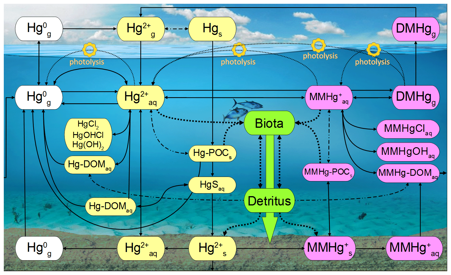
Figure 1Schematic of the chemical mechanism in MERCY. Solid lines indicate chemical reactions, fine dotted lines photolytic reactions, dash-dotted lines instantaneous partitioning processes, and bold dotted lines bioaccumulation and releases from biota into the dissolved phase. Colors codes are white for elemental mercury, yellow for inorganic oxidized mercury, pink for methylated mercury, and green for Hg in biota. The physical state of each species is indicated by “g” for gaseous, “aq” for dissolved, and “s” for solid. The upper row indicates Hg species in the atmosphere, and the lower row indicates those in the sediment. All species and their reactions are given in Tables 2 and 3. Note Reaction (R20) (reductive methylation, Table 3) MMHg–DOM → Hg0 extends to the left edge of the figure.
Table 2Hg species in MERCY. Species can represent state variables in multiple models.
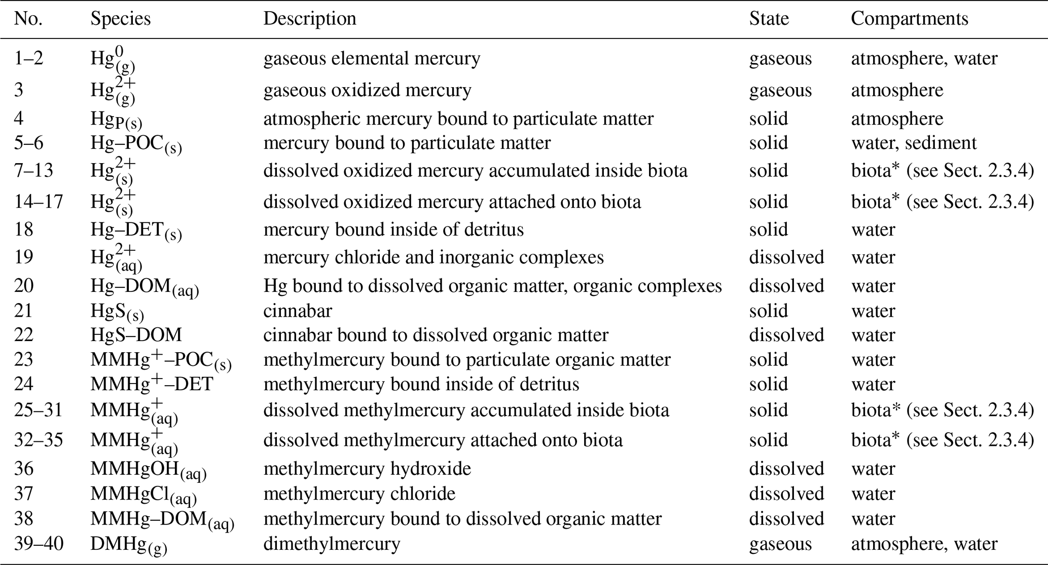
∗ Hg species in biota (Hg and MMHg represent one state variable for each functional group in the ecosystem model ECOSMO (see Sect. 2.3.4), giving a total of 40 mercury species.
2.3.1 Chemistry
In this section, we present all chemical state variables and the transformation processes in the model. A complete overview of all chemical transformations and the respective reaction rates k is given in Table 3. All chemical transformations are calculated using pseudo-first-order reactions following Eq. (7). The chemical mechanism is implemented using a tendency approach, where the relative change for each reaction is calculated and all changes to state variables are applied simultaneously. Equation (3) gives the change to the concentration of a single Hg species due to all reactions depleting and producing it. We run the chemistry module with a time step of 60 s but find that it runs stably and efficiently even with much larger time steps of 600 s.
where Ct is the concentration at time t [ng L−1], C0 is the concentration at time 0 [ng L−1], t is time [s], and k is a pseudo-first-order reaction constant [s−1].
Table 3Chemical reactions as implemented in the MERCY model.
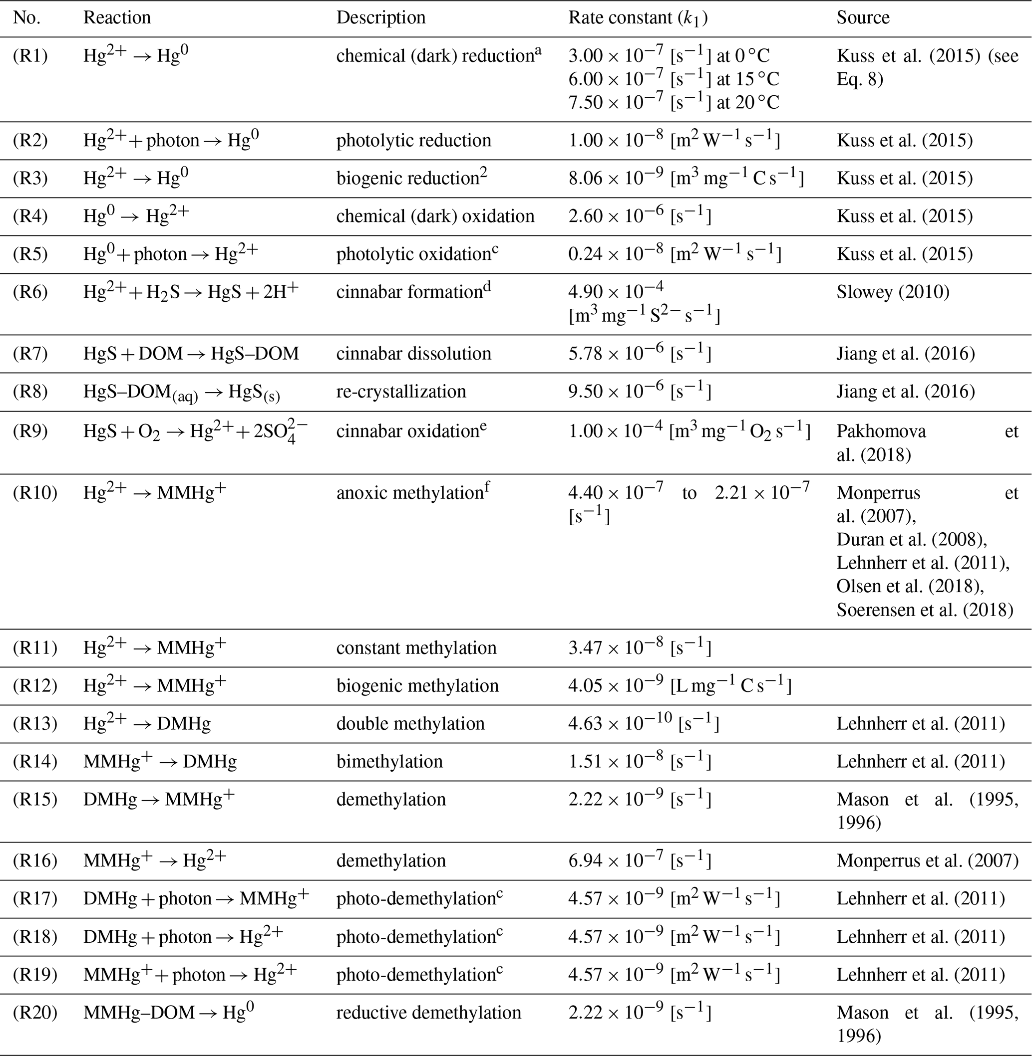
Pseudo-first-order reaction rates k2=k1C depend on the following variables C: a temperature-dependent reaction rate, b cyanobacteria-concentration-dependent reaction rate, c reaction rate dependent on photolytically active radiation, d sulfate-concentration-dependent reaction rate, and e oxygen-dependent concentration reaction rate. f Reaction starts with a lower rate under hypoxic conditions.
Redox reactions
Hg redox chemistry is implemented with five reactions. Reduction (Hg2+ → Hg0) is driven by three processes: (R1) a continuously ongoing chemical reduction, often referred to as dark reduction; (R2) photolytic reduction; and (R3) biogenic reduction (Table 3). We use reaction rates reported by Kuss et al. (2015). This leads to each reduction reaction being of roughly similar importance for the total Hg0 production, albeit with specific distinct seasonality (note that the biogenic reduction only plays a role in the Baltic Sea due to cyanobacteria). This is in contrast to other published reaction rates where photolysis is the dominant pathway (Qureshi et al., 2009). We do not use an intermediate oxidation product (Hg∗) as we found the species to be too short-lived for the given model setup. We chose the values from Kuss et al. (2015) as, contrary to other studies, these were measured under in situ conditions. The oxidation is driven mainly by chemical oxidation (R4), while photolytic oxidation (R5) rates are much smaller, leading to a net photolytic reduction. The photolysis rates are parameterized to the photolytically active radiation based on observations. The biogenic reduction reaction rate is scaled by the cyanobacteria biomass and is not triggered by other phytoplankton species (Kuss et al., 2015). For the chemical reduction, we consider a temperature-dependent reaction rate krd defined as 100 % at 15 ∘C (50 % at 0 ∘C and 125 % at 20 ∘C) (Kuss et al., 2015) (Eq. 8). Finally, we consider reductive demethylation of MeHg+ (Reaction R20), which is only a minor source of Hg0 in the model.
where Tw is the water temperature [∘C] and krd is the dark reduction rate [s−1] (Reaction R1, Table 3).
Cinnabar formation
Additionally, we implemented Hg sulfur chemistry using oxygen concentrations calculated by ECOSMO, whereas sulfur ions (S2−) are represented by negative oxygen concentrations in order to reduce the number of transported state variables (Table 1) (Neumann, 2000). In anoxic waters, cinnabar (HgS) is formed by reaction with sulfide species (H2S, HS−, S2−) (Reaction R6, Table 3). This reaction is kinetically fast and scavenges the majority of the inorganic Hg within a few hours. The product of this reaction is considered particulate but without a sinking velocity due to the small size of these particles (Paquette and Helz, 1995; Soerensen et al., 2018). In the slower Reaction (R7), HgS subsequently binds to −SH groups of DOM, a reaction that can lead to the dissolution of 50 % of the HgS within 24 h. After 1 d, the dissolution reaction is in equilibrium with the re-crystallization Reaction (R8). In the presence of oxygen, sulfur is quickly oxidized and HgS is readily transformed back into soluble Hg species (HgS(s)+ 2O2→ HgSO4 (aq)) (Reaction R9). In the model, HgSO4 is attributed back to the dissolved Hg pool and not tracked by an additional state variable.
Organic chemistry
The organic chemistry doubles the number of variables introduced for the inorganic Hg chemistry mechanism (Fig. 1). In the model, we implemented three sources for MMHg+: (1) methylation in anoxic waters (Reaction R10), (2) methylation in oxic waters (Reaction R11), and (3) methylation due to biologic activity (Reaction R12). The anoxic methylation is thought to be due to anaerobic bacteria and is in our model the fastest methylation process ( s−1). Studies have found that methylation also occurs in oxic waters although at much slower rates (Lehnherr, 2014; Heimbürger et al., 2015; Bowman et al., 2020; Soerensen et al., 2018). We implemented an additional constant methylation reaction ( s−1) and a biologically induced methylation in oxic water to reflect the fact that numerous bacteria have been shown to actively methylate Hg (Soerensen et al., 2018; Capo et al., 2020). We use the amount of remineralized organic material as a proxy for anoxic microenvironments in the oxic water column. The remineralization is dependent on temperature (Eq. 9), with DOM being mineralized at a higher rate of . Following Eq. (7) we calculate the amount of remineralized organic matter and use this to scale the biologic methylation rate (Reaction R12). The reaction rate (Reaction R12) has been chosen such that the effective biological methylation rate mostly lies between Reactions (R10) and (R11), ranging from zero to s−1.
where is the POC remineralization rate [d−1] and Tw is water temperature [∘C].
Besides MMHg+ we also consider double methylation reactions producing DMHg (Reactions R13, R14). For the degradation DMHg → MMHg Hg2+, we consider constant demethylation reactions (Reactions R15, R16), photolytic degradation (Reactions R17–R19), and reductive demethylation (Reaction R20). Finally, we apply methylation and demethylation only to dissolved Hg and MeHg species. Thus, high loads of DOM and POM influence the effective net methylation and produce a non-linear behavior in the system (Olsen et al., 2018).
Chemical reactions in the sediment
In the sediments, we consider only two species: Hg and MMHg. These undergo methylation and demethylation using the same reactions and rates as in the pelagic zone (Table 3). We consider the sediments to always be at least partially anoxic depending on the oxygen concentration in the adjacent water layer (50 %–100 % anoxic for O2 between 2 and 0 mL L−1). All abiotic methylation reactions (Reactions R10 and R11, Table 3) thus take place in the model sediment. Additionally, Hg is subject to dark reduction and subsequently released from the sediment as Hg0 (Capo et al., 2022).
2.3.2 Partitioning
The speciation of Hg2+ and MMHg+ plays a major role in transport, chemical reactions, and bio-availability. In the partitioning scheme we distinguish between three phases: (1) dissolved Hg and MeHg, which are stored in two advected state variables and are further resolved into Hg(OH)2(aq), HgOHCl(aq), HgCl2(aq), MeHgOH(aq), and MeHgCl(aq), which in turn are diagnostic variables dependent on salinity; (2) Hg bound to dissolved organic material Hg2+–DOM(aq) and MeHg+–DOM(aq); and (3) the particulate Hg species Hg2+–POC(s) and MeHg+–POC(s).
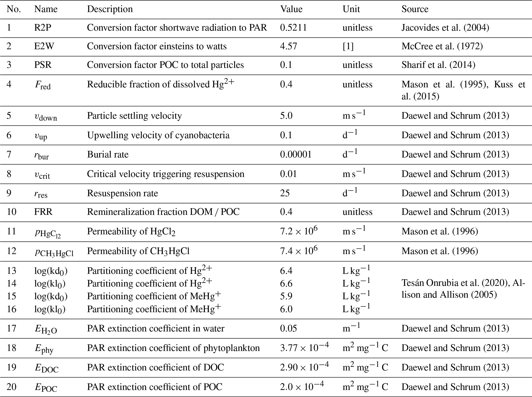
Three-way partitioning is calculated as a function of Hg concentration, particle load, and dissolved organic matter concentration (Eqs. 10–12). As we could not obtain sorption and desorption rates and because our carbon representation does not capture the number of O- and S-binding sites available for Hg, we implemented partitioning based on partitioning coefficients instead of a dynamic sorption/desorption process as described in Eq. (4). We use a value of log(kd)=66 for Hg2+ associated with DOC based on the work of Tesán Onrubia et al. (2020). This kd is higher than what is used in other models (Lyon et al., 1997; Zhang et al., 2019; Kawai et al., 2020). Moreover, we use distinct partitioning coefficients for binding to POC kd and DOC kl for inorganic Hg2+ (log(kd) = 5.4 L kg−1 and log(kl)=5.6) and organic MMHg+ (log(kd)=4.9 and log(kl)=5.0) (Allison and Allison, 2005; Batrakova et al., 2014) (Table 4).
Here, kd is the Hg–POM(s) Hg(aq) partitioning coefficient [1], kl is the Hg–DOM(aq) Hg(aq) partitioning coefficient [1], POM denotes particulate organic matter [1], SPM denotes suspended particles [1], and DOM denotes dissolved organic matter [1].
The model assumes instantaneous equilibrium and redistributes Hg2+ and MeHg+ between the three states on each time step. This approach is supported by lab studies that indicate the partitioning equilibrium is reached within an hour (Mason et al., 1995). Finally, mass conservation is ensured by Eq. (12).
2.3.3 Radiation
The radiation available for photolytic reactions is determined from hourly input fields using shortwave radiation reaching the surface as modeled by the meteorological model COSMO-CLM (Table 1). As the reaction rates for Hg photolysis are usually reported in relation to photolytically active radiation (PAR), we convert the modeled shortwave radiation using an average factor of 0.5211, not taking into account diurnal variations (Jacovides et al., 2004). We then calculate the cumulative light extinction Etot (Eq. 13) by water (Eq. 14), phytoplankton (Eq. 15), dissolved organic matter (Eq. 16), and suspended particles (SPM) (Eq. 17), whereby we estimate the total particulate matter concentration for light attenuation using a constant ratio of 0.1 times the particulate organic carbon (POC) concentration (Sharif et al., 2014) (Eq. 18). Finally, the remaining radiation Rz at half the depth of each layer is calculated following the Lambert–Beer law (Eq. 19). All parameters used to calculate light extinction are given in Table 4.
Here, CFLA is the flagellate concentration [mg C m−3], CDIA is the diatom concentration [mg C m−3], CCYA is the cyanobacteria concentration [mg C m−3], CDOC denotes dissolved organic carbon [mg C m−3], CPOC denotes particulate organic carbon [mg C m−3], CP total denotes the total particle load [mg C m−3], PSR denotes the POC fraction of total particles [1] = 0.1 (Sharif et al., 2014), Ephy denotes extinction by phytoplankton [1], EDOC denotes extinction by DOC [1], EPOC denotes extinction by POC [1], denotes extinction by water [1], Etot denotes total light extinction [1], z is the number of vertical layers [1], n is the number of layers [1], h is the height of grid cell z [m], and R is radiation at layer z+1 [W m−2].
2.3.4 Biological uptake
Hg bioaccumulation has been implemented directly into the HAMSOM-ECOSMO framework (Daewel and Schrum, 2013; Daewel et al., 2019). ECOSMO is based on a functional group approach lumping species based on properties like nutrient requirements (NO, NH, PO, SiO2) and feeding habits (herbivorous, omnivorous, carnivorous). ECOSMO includes three phytoplankton species (flagellates, diatoms, and cyanobacteria) and two zooplankton species (micro- and mesozooplankton), as well as a macrobenthos and a fish group with the latter representing mass fluxes to higher trophic levels (Fig. 2).
In MERCY we consider bioaccumulation of inorganic Hg2+ and organic MeHg+ for each of the seven functional groups. Moreover, we distinguish between passive uptake directly from the water column (bioconcentration) and active uptake due to the consumption of contaminated food (biomagnification). The first is accumulated as Hg attached to the organism (zooplankton carapace, fish gills) and the second incorporated internally. Figure 3 depicts a schematic overview of the rate constants used to describe bioaccumulation in MERCY with phytoplankton, which only undergoes passive uptake, on the left and with higher trophic species, which also actively feed on other species, in the middle and on the right. All bioaccumulation processes are calculated separately for inorganic Hg2+ and organic MeHg+, and the accumulated Hg is transported consistently with the movement of the associated biota. In total, this leads to 22 bioaccumulation state variables (6 phytoplankton, 8 zooplankton, 4 macrobenthos, and 4 fish), which roughly doubles the number of chemical state variables (20) in the model (Table 2). All parameters used for bioaccumulation modeling are given in Table 5.
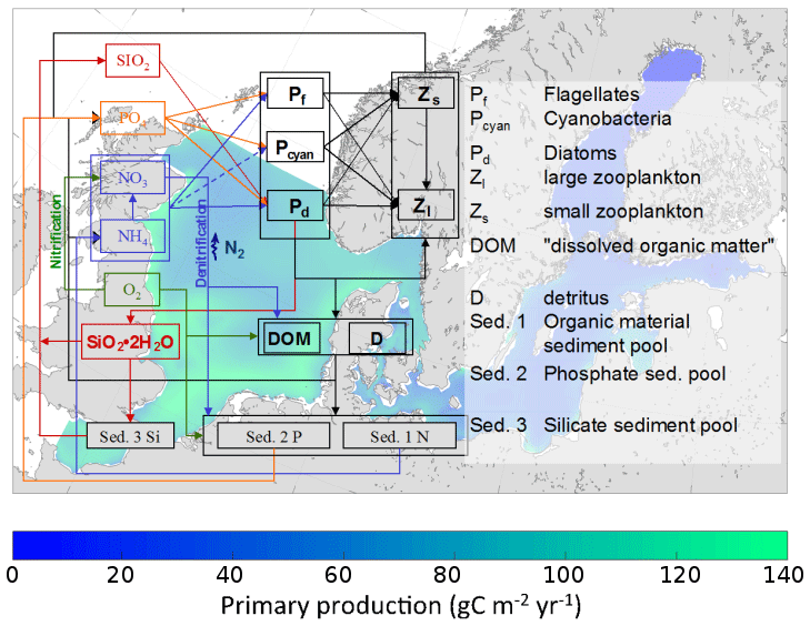
Figure 2Overview of the ECOSMO marine ecosystem nutrient and functional group model (Daewel et al., 2019).
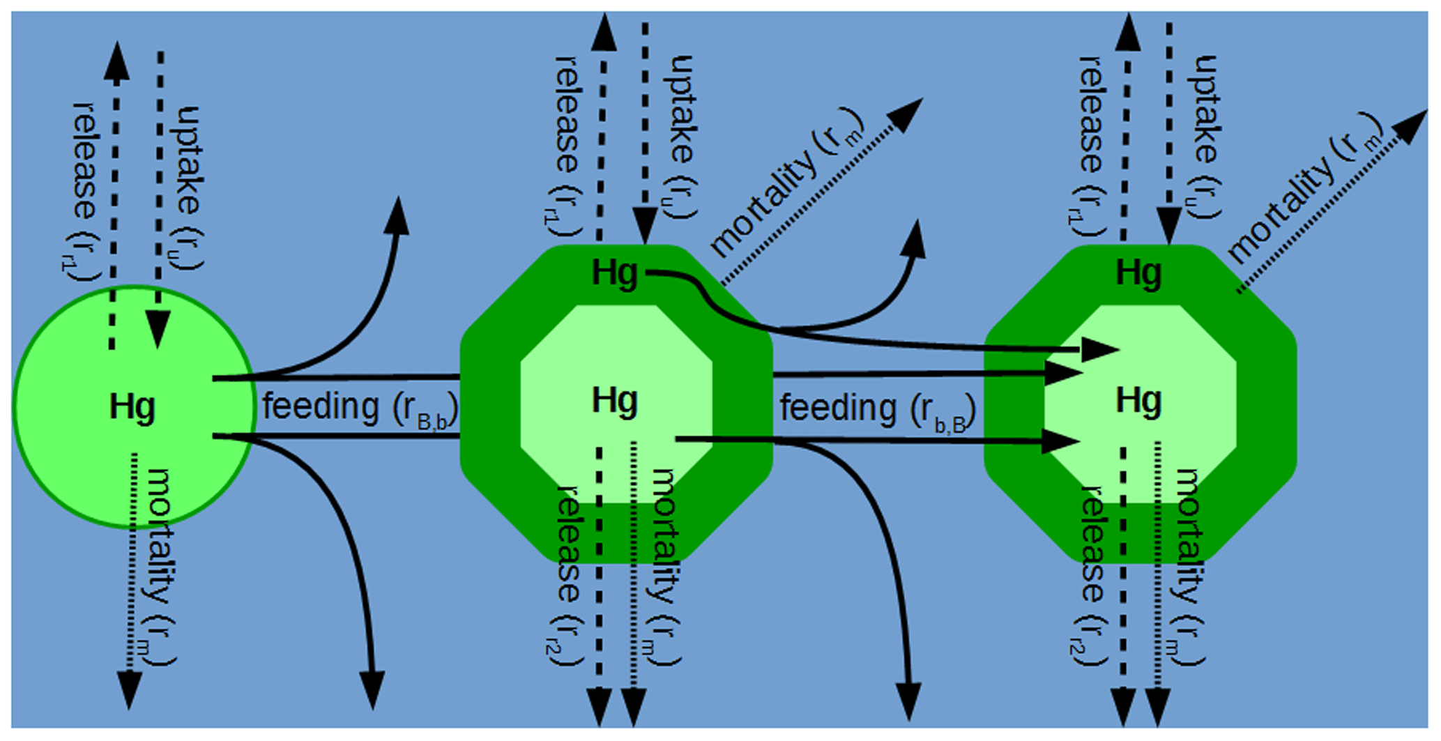
Figure 3Schematic overview of Hg2+ and MMHg+ bioaccumulation for phytoplankton (left), microzooplankton (middle), and mesozooplankton (right). Dashed lines indicate passive uptake and release rates (Eq. 19); solid lines indicate active uptake due to feeding, with a fraction being instantly released back into the water column (Eq. 22); and dotted lines show Hg loss due to mortality (Eq. 23).
Bioconcentration
In MERCY dissolved Hg and MMHg are accumulated via passive uptake UP (Eq. 20) through the cell membrane of the phytoplankton functional groups (diatoms, flagellates, cyanobacteria). For zooplankton, macrobenthos, and fish, the passive uptake is thought to lead to Hg accumulation on the surface or areas that are exposed to water like the mouth or gills in the case of fish (Fig. 3: ru). The uptake rate is ru calculated based on the surface area A(B) dependent on an ecosystem functional group B and a Hg-species-dependent permeation velocity v (Eq. 21). We estimate average volume and surface areas for phytoplankton species based on observations of size and geometric shape (Table S1) (Olenina et al., 2003). The cell volume is used to estimate the organic carbon content, which is then used to estimate the ratio of organic carbon to the cell surface (Menden-Deuer and Lessard, 2000). This ratio allows us to model the total phytoplankton cell surface per functional group based on the organic carbon content as modeled in ECOSMO. The estimated surface area is used to calculate the Hg-species-dependent uptake rate based on Mason et al. (1996). Diffusive uptake by zooplankton is implemented based on experimental uptake studies but is less important compared to phytoplankton due to the comparably small surface areas of these species (Tsui and Wang, 2004).
where UP (B) is the passive uptake of ecosystem group B [ng s−1], ru is the passive uptake rate [s−1], and Hg is dissolved Hg [ng m−3].
where vC is the permeation velocity for Hg species i [m s−1], AB is the average surface area of ecosystem group B [m2 mg−1 C], and CB is the concentration of ecosystem group B [mg C m−3].
Biomagnification
For all non-phytoplankton species, we consider the active uptake UA due to feeding rates rB,b and rb,B which lead to a fraction ϵ(C) of the Hg in prey to be incorporated into the predator (Fig. 3: rB,b rb,B). Through this process, Hg2+ and MMHg+ are magnified along the food web (Eq. 22). Zooplankton feeds on detritus, phytoplankton, and other zooplankton, while fish feed on mesozooplankton and macrobenthos following Daewel et al. (2019) (Fig. 4). Moreover, there is macrobenthos that exists only in the marine bottom layer and feeds on these species. We base our uptake on studies that show that only a fraction of Hg2+ (ϵ(Hg)=0.45) and a fraction of MMHg+ (ϵ(MeHg)=0.97) are incorporated into the predator, while the rest is excreted directly back into the water column (Mason et al., 1996; Wang and Wong, 2003; Tsui and Wang, 2004; Pickhardt et al., 2006).
where UA (B) is the active uptake rate in ecosystem group B [ng s−1], HgB is the Hg concentration in ecosystem group B [ng m−3], Hgb is the Hg concentration in ecosystem group b [ng m−3], m is the number of ecosystem groups [1], rB,b is the feeding rate [m3 s−1], rB,b is the predation rate [m3 s−1], and ϵC is the feeding efficiency [dimensionless between 0–1].
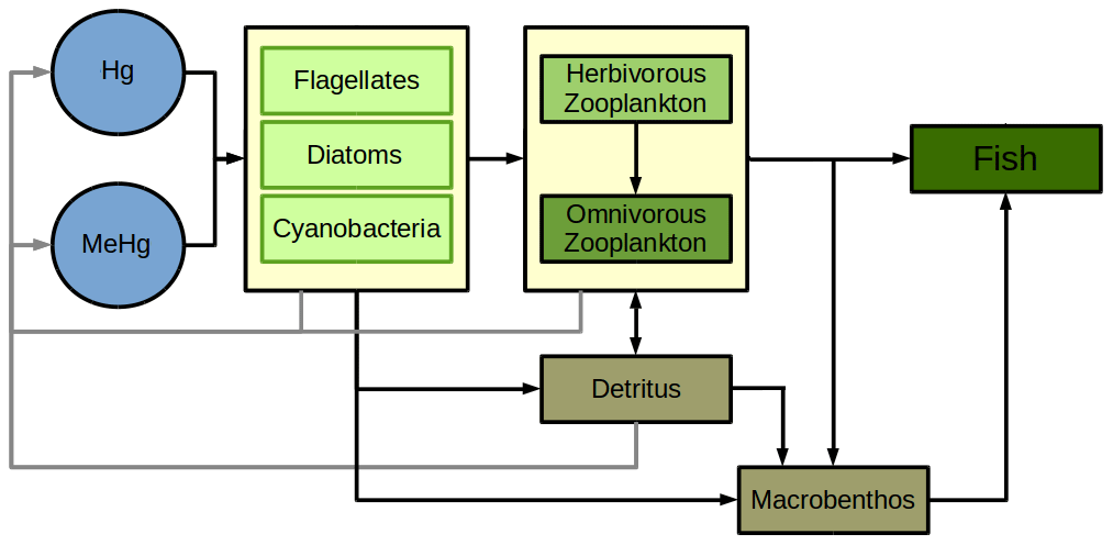
Figure 4Flowchart of Hg bioaccumulation due to feeding following the ECOSMO end-to-end functional group approximation (Daewel et al., 2019). Rates for all depicted flows are given in Table 5.
Release
Mercury accumulated by active UA and passive uptake UP can also be released back into the water column (Eq. 23). There are three distinct processes in the bioaccumulation model that release Hg accumulated in the food web back into the water column. Firstly, there are species-dependent fixed release rates for Hg adsorbed to (rr1) and adsorbed in (rr2) the biological species (Eq. 25). Secondly, upon feeding described by feeding rates rB,b and rb,B, a fraction 1−ϵ(C) of the Hg accumulated in prey is not incorporated into the predator, and this is directly released back into the water column (Eq. 24). Finally, based on the ECOSMO mortality and respiration rates rm for each ecosystem group, Hg is released (Eq. 26). Feeding, mortality, and respiration rates are directly taken from ECOSMO (Table 1), and the relevant equations are described in detail in Daewel et al. (2019). For detritus, the mortality rate is a temperature-dependent remineralization rate (Eq. 9).
where R(B) is the release rate from ecosystem group B [ng s−1], RR(B) (Eq. 24) is the constant release rate [ng s−1], RF(B) (Eq. 25) is the feeding-related release rate [ng s−1], and RM(B) (Eq. 26) is the mortality-related release rate [ng s−1].
where Hg(b) ext is Hg on ecosystem group B [ng m−3], Hg(b) int is Hg inside ecosystem group B [ng m−3], rr1 is the release rate of external Hg [m3 s−1], and rr2 is the release rate of internal Hg [m3 s−1].
where rB,b is the feeding rate of group B on group b [s−1], ϵC int is the feeding efficiency for external Hg species C [dimensionless between 0–1], ϵC ext is the feeding efficiency for external Hg species C [dimensionless between 0–1], Hg(b) ext is Hg on ecosystem group b [ng m−3], and Hg(b) int is Hg inside ecosystem group b [ng m−3].
where rm is the mortality rate of ecosystem group B [m3 s−1].
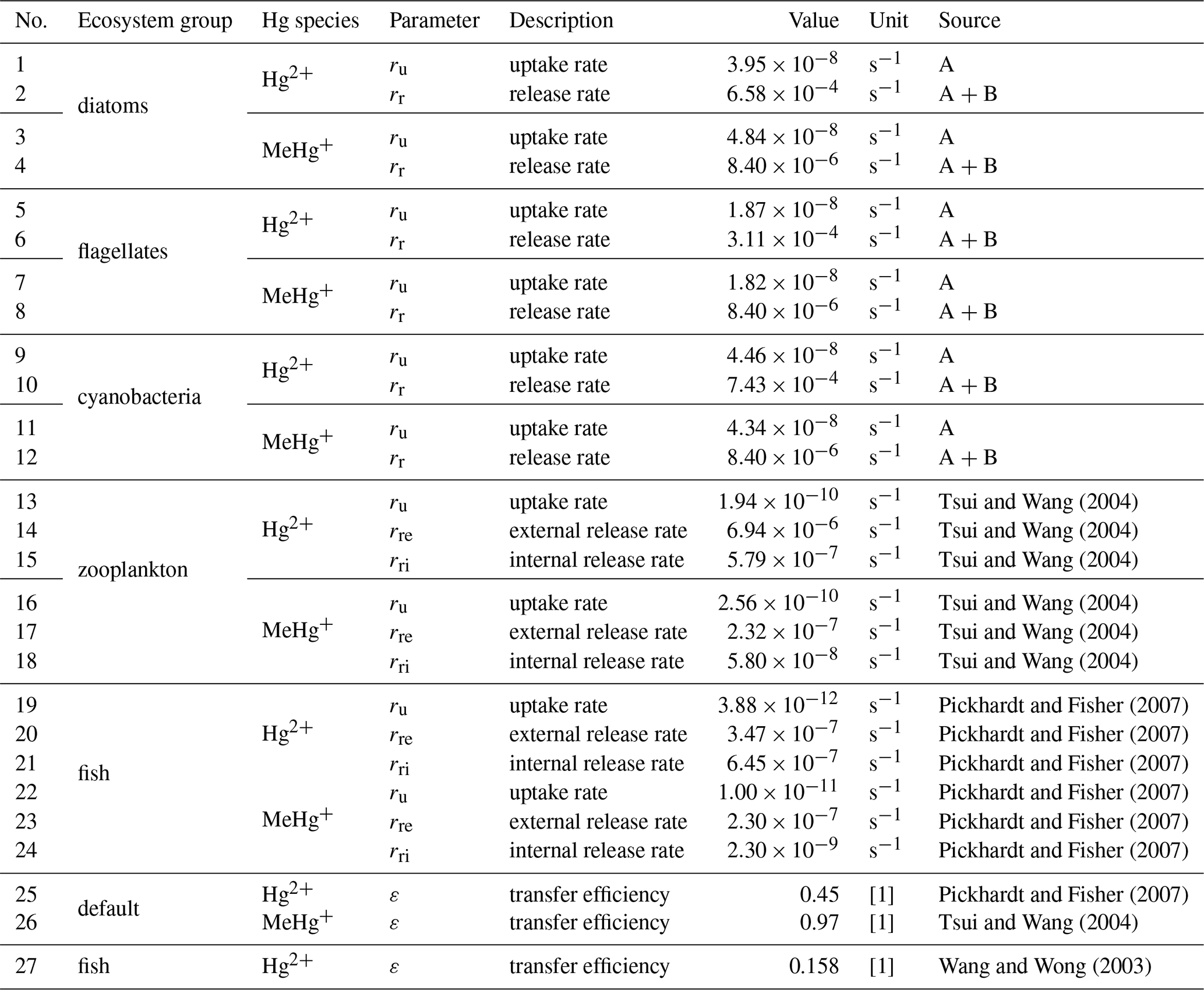
Table 5Overview of bioaccumulation parameters. External variables taken from the ecosystem model ECOSMO such as mortality (rm) and feeding rates (rf) are given in Table 1. The abbreviated phytoplankton references are (A) Mason et al. (1996), Menden-Deuer and Lessard (2000), and Olenina et al. (2003) and (B) Pickhardt and Fisher (2007) and Nfon et al. (2009).
2.3.5 Benthic–pelagic coupling
Following the sediment modeling concept by Daewel et al. (2019), we implemented a simple two-layer sediment system, where the first layer interacts with the lowest water column grid cell and the second layer represents a permanent sink.
Sedimentation
Sedimentation occurs due to the settling of Hg bound to particles and detritus. The sedimentation flux Fs is calculated using a sinking velocity wd of 5 m d−1 for Hg bound to particles (POC) (Daewel and Schrum, 2013) (Eq. 27).
where FS is the sedimentation flux [ng s−1 m−2], Hg is the particulate mercury concentration in water [ng m−3], and wd is the sinking velocity [m s−1].
Resuspension
Resuspension Fr is triggered by a critical ocean current velocity of U 0.01 m s−1. In the case that a critical current velocity is reached, no sedimentation takes place and a resuspension rate rres of 25 [d−1] is used to release Hg from the first sediment layer into the lowest water grid cell (Eq. 28). Depending on the depth (<1 m) of the lowest grid cell and current velocity, resuspension can also directly affect the second-lowest water grid cell.
where Fr is the resuspension flux [ng s−1 m−2], rres is the resuspension rate [s−1], and Hg is the mercury concentration in sediment [ng m−2].
Burial
Hg2+ and MMHg+ in the first layer are constantly transported to the second layer, which represents a permanent sink in the model. The burial flux Fb is based on a constant burial rate of kbur= [d−1] (Eq. 29, Table 4).
where Fb is burial flux [ng s−1 m−2], rbur is the burial rate [s−1], and Hg is the mercury concentration in sediment [ng m−2].
2.3.6 Air–sea exchange
Air–sea exchange of elemental Hg0 is one of the most important processes in the global Hg cycle. Here, we use the approach of Kuss et al. (2009), Kuss (2014)), which is based on Henry's law constant H by Andersson et al. (2008) to determine the equilibrium between Hg0 in water and air (Eq. 30). Next, the transfer velocity for CO2k600 is approximated using a quadratic parameterization depending on the 10 m wind speed U10 (Eq. 31). We then calculate the transfer velocity kw for Hg0 by scaling k600 using the temperature (T)-dependent and salinity (S)-dependent diffusivity of Hg0 in water (Eqs. 32 to 35) (Kuss, 2014). The actual inter-compartmental Hg0 flux FHg is then calculated based on surface concentrations in the adjacent compartments (Eq. 36). The air–sea exchange is also applied for DMHg. However, the CMAQ-Hg model does not consider DMHg yet. Hence, the atmosphere is only a sink for DMHg, which is instantaneously transformed into Hg2+ (Niki et al., 1983), and its fate is currently not explicitly resolved.
(Anderssen et al., 2008)
(Nightingale et al., 2000)
(Kuss, 2014)
(Kuss, 2014)
(Kuss, 2014)
(Kuss, 2014)
(Schwarzenbach et al., 2003)
In the above equations (Eqs. 30–36), HHg is Henry's law constant [1], T is water temperature [∘C], S is salinity [PSU], Sc35 is the Schmidt number for salt water [1], Sc0 is the Schmidt number for fresh water [1], k600 is the transfer velocity of CO2 [cm h−1], kw is the transfer velocity of Hg [cm h−1], Hg is the Hg0 concentration in air [ng m−3], Hg is the Hg0 concentration in water [ng m−3], and FHg is the net Hg0 flux from atmosphere to water [ng m−2 h−1].
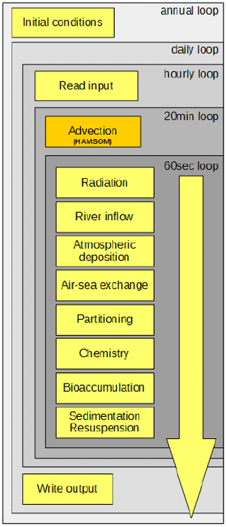
2.3.7 Technical implementation
As a basis for the presented model development, we build upon the setup used for the earlier-published inorganic marine Hg model MERCY (Bieser and Schrum, 2016). All processes are implemented as stand-alone routines which are called from a main driver function containing several time loops (Fig. 5). Data for the wet cells (pelagic) are stored in vector form to reduce overhead, and data for sediments (benthic) and the lowest atmospheric layer are stored in 2D fields. Input data (Table 1) are read directly during run time from binary ECOSMO output as hourly mean values. This approach was chosen because there is no feedback from the Hg chemistry on the physical and biological models and because it allows us to reduce the computational costs of running the marine Hg model. All output files are created with daily mean values and saved in netCDF format using the IO-API interface (Byun and Schere, 2006; IO-API). The model is set up in a way that it runs for a single year using the last output time step of the previous year as an initial condition. For this initial model evaluation, we run MERCY for 17 years from 2000 to 2016.
We determine the model performance in reproducing observed concentrations and dynamics (e.g., variability and seasonality) of individual Hg species. Based on this analysis, we identify the processes and parameters responsible for the model error. The model is not specifically calibrated to the area of application, the North and Baltic seas. It is built on the current understanding of mercury cycling in the ocean and should be generally applicable. Major factors that need to be considered before applying the MERCY model to other regions are (1) partitioning coefficients for organic material (OM) as the type of OM varies regionally, (2) the parameterization for biogenic reduction as the values presented here are based on cyanobacteria in the Baltic Sea, (3) the uptake and release rates for bioaccumulation which might not be representative of other regions, and (4) the ecosystem model used that is needed to drive MERCY.
3.1 Statistics
Because there are no established quality criteria for marine models, we use criteria commonly used for evaluation of atmospheric CTMs (Derwent et al., 2010; Thunis et al., 2012, 2013; Carnevale et al., 2014). We start by comparing the observed and predicted means (Eq. 37) using daily model averages in the 10×10 km2 grid cell corresponding to the observation. As statistical metrics, we use bias (Eq. 38), error (Eq. 39), standard deviation (Eqs. 40, 41), and the correlation coefficient (Eq. 42) to evaluate systematic error, random error, amplitude error, and phase error. However, for most Hg species, the observations lack the temporal coverage to determine the phase error. Moreover, we use the centered root-mean-square error (CRMSE) because it allows us to distinguish between systematic error (bias) and random error (CRMSE) (Eq. 43) (Carnevale et al., 2014). For our analysis, we normalize the statistical metrics to get concentration-independent values and allow for better comparability between different Hg species.
Equation (37) gives the mean.
where Pi is the predicted value from the model, Oi denotes observed values from measurement, N is the sample size/number of observations, and i is the index.
Equation (38) gives the normalized mean bias.
Equation (39) gives the normalized centered root-mean-square error.
Equation (40) gives the standard deviation.
Equation (41) gives the normalized mean standard deviation.
Equation (42) gives the correlation coefficient (r).
Equation (43) gives the root-mean-square error.
Finally, we use additional quality criteria to determine model performance: firstly, the percentage of model values within a factor of 2 (FAC2), which gives an easy-to-understand estimate of the model quality (Eq. 44). We argue that model values within a factor of 2 are within the combined uncertainty. The uncertainty consists of the measurement uncertainty, the sampling uncertainty when comparing observations with time-integrated (24 h) and space-integrated (100 km2) model grid cells (Schutgens et al., 2016), and the error propagation in the biogeochemical modeling framework. We estimate the measurement error U to be in the range from 20 % for Hg0 and HgT to 50 % for MeHg.
Equation (44) gives the factor of 2.
with ni=1 for and otherwise ni=0.
Secondly, we use the more technical model quality objective (MQO) as defined by Carnevale et al. (2014). The MQO (Eq. 45) relates the root-mean-square error (Eq. 46) to the root-mean-square uncertainty (Eq. 47). The MQO can be interpreted as follows: for MQO<0.5 on average the model values lie within the measurement uncertainty and thus the model cannot be improved upon unless more precise observations become available. For MQO>1 the model error is on average larger than the measurement uncertainty but the model may be closer to the “true” environmental value than the observations. Thus, the aim is to achieve an MQO<1. Moreover, we determine model performance criteria for NMB, NMSD, and RMSE as proposed by Carnevale et al. (2014) (Eqs. 49–51).
Equation (45) gives the model quality objective.
Equation (46) gives the root-mean-square error.
Equation (47) gives the root-mean-square uncertainty.
where U denotes the measurement uncertainty.
Equation (48) gives the model performance criterion for NMB.
Equation (49) gives the model performance criterion for NMSD.
Equation (50) gives the model performance criterion for RMSE.
These quality criteria have been developed for atmospheric pollutants like ozone, nitrogen oxides, and fine particles, which have been studied and modeled for decades. For modeling of Hg in the marine environment, the observations are still very limited compared to those of pollutants in the atmosphere. This affects the ability to use these criteria, and we therefore do not expect the MERCY model to meet the criteria at this point. However, we define these as our future goal for marine Hg modeling.
3.2 Model domain (North Sea and Baltic Sea)
Here, we evaluate the model for the North and Baltic seas in northern Europe (model domain shown in Fig. 6). This area was chosen for model evaluation as it covers a large range of different physical and biological conditions: the Baltic Sea (Fig. 6; marine regions 8–15) is an enclosed shelf sea with a surface area of 377 000 km2. It is connected to the North Sea (marine regions 1–5) via the shallow Kattegat and Skagerrak (marine regions 6–7) in the southwest. It is a brackish waterbody strongly influenced by freshwater inflow, and it covers a salinity range from <2 PSU in the north that increases towards the southwest to up to 35 PSU in the transition zone between the North and Baltic seas (Fischer and Matthäus, 1996; Lehmann and Post, 2015; Mohrholz et al., 2015). The central Baltic Sea has several deep basins reaching a depth of 460 m in the Landsort Deep (Fig. 6b). It exhibits strong stable stratification with more saline, in parts anoxic, deep water, resulting from an estuarine circulation system with upper-layer outflow of fresh water and lower-layer saline inflow. Every few years, large quantities of oxic and saline waters are transported from the North Sea to the Baltic Sea during so-called major Baltic inflows (MBIs). During the simulation period 2000 to 2015, three MBIs occurred; one of these was an especially strong event during the winter of 2014/15 (Fischer and Matthäus, 1996; Lehmann and Post, 2015). In the northern part of the Baltic, the Bothnian Sea and the Bothnian Bay are seasonally covered by ice, possibly leading to accumulation of Hg from rivers during winter due to the suppression of Hg0 evasion. Finally, the Baltic Sea is a system with cyanobacteria, which makes it an interesting study area as these cyanobacteria have been shown to actively reduce Hg (Kuss et al., 2015). Moreover, cyanobacteria can lead to pronounced early-spring–late-summer biomass blooms that affect bioaccumulation (Soerensen et al., 2016a).
The North Sea has a surface area of 575 000 km2 and is connected to the Atlantic Ocean at its northern border and via the English Channel to the south. It is a shallow shelf ocean that is well mixed during autumn and winter, and it experiences frequent resuspension events during autumn and winter storms. The southern North Sea is characterized by strong tidal mixing, and thus water masses are well mixed and sediments are resuspended regularly within the tidal cycle. It is an area of high primary productivity and an important fishing ground. Thus, it is an important study area for Hg methylation and bioaccumulation.
Due to their close vicinity to the coast and national monitoring programs, there are a comparably large number of Hg observations available for both the North Sea and the Baltic Sea. However, the data on Hg are still sparse in some areas, especially regarding Hg speciation, which is a major obstacle for model evaluation.
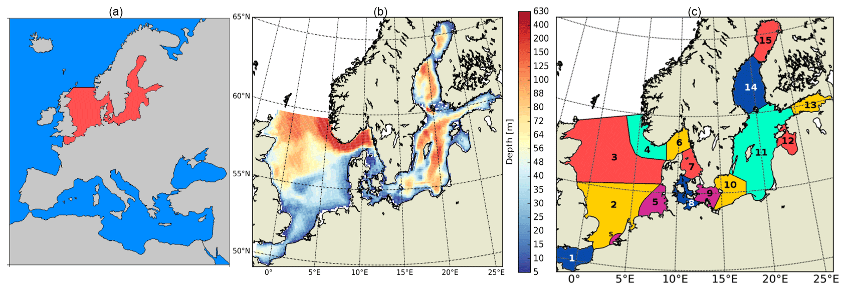
Figure 6(a) COSMO-CMAQ-Hg atmospheric model domain with the North and Baltic seas highlighted. (b) MERCY marine model domain and topography. (c) Marine regions: (1) English Channel, (S) Scheldt Estuary, (2) southern North Sea, (3) northern North Sea, (4) Norwegian Trench, (5) German Bight, (6) Kattegat, (7) Skagerrak, (8) Belt Sea, (6–8) Swedish west coast, (9) Arkona Sea, (10) Bornholm Sea, (11) Gotland Sea or Baltic Proper, (12) Bay of Riga, (13) Neva Bay, (14) Bothnian Sea, and (15) Bothnian Bay.
3.2.1 Forcing data
To generate the necessary forcing data (Table 1) to run the MERCY model, we used the four models described in Sect. 2.1. For the atmosphere, COSMO-CLM was run on a regional domain for Europe driven by ERA-Interim re-analysis data (Berrisford et al., 2011; Dee et al., 2011; Hersbach et al., 2020). The atmospheric model domain covers the entire European landmass, including northern Africa and western Russia, with a resolution of 24×24 km and 35 vertical layers (Fig. 6a). The calculated meteorology is then used as forcing for the atmospheric CTM CMAQ-Hg, which is set up for the same domain and resolution (Byun and Schere, 2006; Zhu et al., 2015; Bieser et al., 2016). CMAQ-Hg uses boundary concentrations for Hg by an ensemble of the global Hg models GEOS-Chem, GLEMOS, ECHMERIT, and GEM-MACH-Hg (Travnikov et al., 2017) and all other relevant trace gases from the global CTM MOZART (Horowitz et al., 2001). Emissions for the year 2010 were created with the SMOKE-EU emission model (Bieser et al., 2011). Hg emissions are based on the AMAP emission inventory (AMAP/EMEP, 2019b). This is a similar setup to that used in previous studies (Bieser and Schrum, 2016). For computational reasons, we calculated only 1 year (2010) of atmospheric Hg concentration and deposition fields. These were used as boundary conditions for the marine Hg model for all years of the simulation. The ocean-ecosystem model HAMSOM-ECOSMO was run on a model domain covering the entire Baltic Sea and the North Sea with open boundaries in the English Channel and at 63∘ N, where the North Sea is connected to the Atlantic (Fig. 6b). The resolution of the model is about 10×10 km2 (spherical grid) with 20 layers and a maximum water depth of 630 m. The vertical resolution is 5 m for the four uppermost layers with a bottom layer depth of 250 m.
3.2.2 Initial conditions
As initial conditions, we interpolated observations in water, biota, and sediment using a traditional kriging methodology to produce realistic initial starting conditions (mostly the pronounced vertical gradient) and minimize the spin-up time required (Cressie, 1990). The observational Hg data were retrieved from the database of the German Federal Maritime and Hydrographic Agency (MARENET, 2020). We ran the model using initial conditions multiplied by factors of 0.5 and 2.0 and tested the time necessary for the two runs to converge. For our model domain, which is a relatively small and in parts enclosed shelf sea area, the model runs started to converge after only a few years in the water column but took several years for Hg in sediments and biota (especially at higher trophic levels). For this study, we used a spin-up time of 30 years to reach realistic initial conditions for the production runs.
3.2.3 Boundary conditions
The chosen domain, including only the North Sea and Baltic Sea, has only a very small open boundary: the English Channel in the southwest, which forms a narrow connection to the Atlantic Ocean, and the wider opening in the northern channel. The North Sea in the north of the domain, which receives most of the Atlantic inflow, is connected to the open Atlantic Ocean at the shelf break. This region is characterized by an outflow in the eastern part and inflow in the western part. At the open boundaries, we prescribe constant Hg concentrations using 1.0 pM HgT for the North Atlantic and 3.0 pM HgT in the English Channel (Cossa et al., 2018; Leermakers et al., 2001).
3.2.4 River loads
River loads are taken from OSPAR and HELCOM reports and the Norwegian Tilførsel program (Green et al., 2011; HELCOM, 2007, 2011). We implemented rivers using monthly load data in the North Sea and annual values for the Baltic Sea as described in Bieser and Schrum (2016). The annual inflow of Hg through rivers is 1100 kg a−1 for the Baltic and 2800 kg a−1 for the North Sea. In the North Sea, the largest fluxes are from the Elbe (1160 kg a−1) and Rhine (800 kg a−1) rivers.
3.2.5 Deposition of Hg2+ and atmospheric Hg0
Dry and wet Hg deposition is read in as hourly totals from CMAQ netCDF output files. The deposited Hg and Hg are added to the dissolved Hg species assuming instant dissolution of atmospheric particles. In CMAQ, the exchange of Hg0 is set to zero for all grid cells with the land-use category water to avoid a doubling of the air–sea exchange calculation in the atmospheric model.
3.3 Observational data
For the model performance, we start by evaluating total Hg (HgT) concentrations in the water column. We then look at the individual species, elemental Hg0 and organic MeHg. Next, we evaluate the model skill in reproducing Hg concentrations in biota. For this, we compare Hg and MeHg loads in phytoplankton and zooplankton and finally total Hg in fish (HgFish).
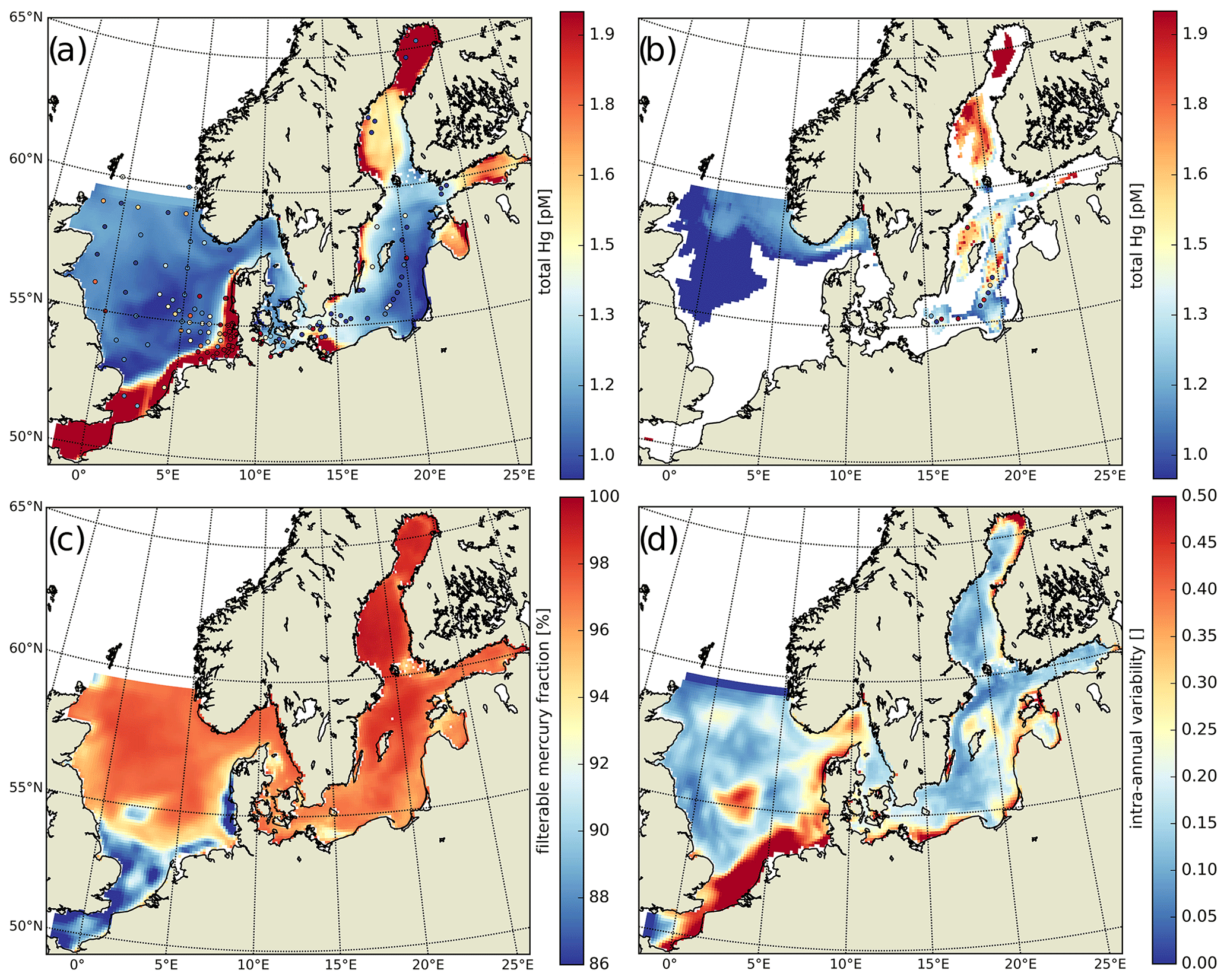
Figure 7Annual averages: (a) HgT concentrations in the top 50 m with superimposed observations (Kuss et al., 2017; Soerensen et al., 2018; MARENET, 2020), (b) HgT concentrations below 50 m with superimposed observations, (c) average fraction of filterable HgFilt. as a proportion of HgT, and (d) intra-annual variability in modeled daily average HgT concentrations.
3.3.1 Total Hg in water
The available HgT observations cover offshore and coastal areas in the North and Baltic seas. HgT has been measured as both unfiltered (Soerensen et al., 2018) and the filterable fraction HgFilt. (Kuss et al., 2017; MARENET, 2020). In MERCY, HgFilt. corresponds to the sum of eight species, namely Hg, Hg, Hg–DOM(aq), HgS–DOM(aq), MMHg, MMHg–DOM(aq), DMHg(g), and HgS(s) (Table 2). HgT additionally includes HgP, which is comprised of the two particulate species Hg–POC(s) and MeHg–POC(s). In our model HgFilt. makes up about 95 % of HgT on average (Fig. 7c). HgP only plays a significant role (>5 % on annual average) in the southern North Sea and the Wadden Sea. Especially in the Wadden Sea, observed HgT concentrations are extremely high with values ranging from 6 to 117 pM. For the model performance evaluation, we removed measurements taken in the Wadden Sea and other areas not resolved in our model setup (e.g., the area between the coastline and barrier islands and lagoons in the Baltic Sea). As depicted in Fig. 7a, virtually no observations are from regions where particles play a major role. Thus, for simplification we will use the term HgT to refer to all of these observations, but we compare them to concentrations of the respective model species.
In the North Sea we use 435 measurements of HgT sampled between 2007 and 2011 (MARENET, 2020). The samples are taken over the entire year, but BSH (the German Federal Maritime and Hydrographic Agency) sampling focuses mostly on the German exclusive economic zone, although it also includes a few years with data for the greater North Sea. Finally, all measurements are surface samples (0–20 m), which is due to the shallow nature of the North Sea. For the Baltic Sea, there are 111 observations from the MARENET database (MARENET, 2020); 168 observations from three cruises in March 2014, March 2015, and July–August 2015, which cover the southern part of the Baltic Sea from the Belt Sea to the Gotland Deep (Kuss et al., 2017); and 90 observations from three cruises in July and August of 2015 and 2016, which in addition include observations on the Bothnian Sea and Bothnian Bay (Soerensen et al., 2018). Figure 7a and b depict all HgT observations used for model evaluation.
3.3.2 Individual marine species: Hg0 and MMHg+
For the evaluation of Hg0, we use 580 measurements from four Baltic Sea cruises in February, April, July, and November 2006 (Kuss, 2014). This dataset allows us to investigate the seasonality of redox reactions. For MMHg+, we were able to obtain 310 measurements from six cruises in 2014, 2015, and 2016 covering coastal and offshore areas of the Baltic Sea (Kuss et al., 2017; Soerensen et al., 2017, 2018). For 160 of these, both MeHg and HgT were available, which enables a relative evaluation of the methylated fraction Mfrac= MeHg HgT. For the North Sea, no Hg0 or MMHg+ observations are available at all with the exception of nine MeHg measurements from 1999 in the English Channel and the Scheldt Estuary, which we used to set the MMHg+ boundary conditions in the English Channel (Leemakers et al., 2001). Thus, we are forced to limit the model evaluation for Hg0 and MMHg+ to the Baltic Sea.
3.3.3 Hg in biota
Bioaccumulation in the marine biota is evaluated by comparing their total Hg and MeHg content to measured concentrations in biota in the Baltic Sea (Nfon et al., 2009). For evaluation of fish total Hg, we use HgT concentration in the muscle tissue of 1166 herring from coastal and offshore locations in the Baltic Sea (Soerensen and Faxneld, 2020). As the biota measurements are in wet weight and our model is in milligrams of carbon dry weight, the ratio of milligrams of carbon per milligram biota of 0.2 for diatoms, 0.33 for flagellates and cyanobacteria, and 0.5 for zooplankton and fish was assumed (Sicko-Goad et al., 1984; Walve and Larsson, 1999). This was combined with a conversion factor of dry weight to wet weight of 0.2 for phytoplankton, 0.16 for zooplankton, and 0.1 for fish (Cushing, 1958; Ricciardi and Bourget, 1998). For phyto- and zooplankton, the model is compared to the observed average, minimum, and maximum concentrations, but due to limited data, no seasonal or regional comparison was possible. For fish we analyze Hg accumulation for five Baltic Sea regions ranging from the western Baltic to the Bothnian Bay.
3.4 Model performance
3.4.1 North Sea (HgT)
Figure 8 compares the frequency distribution of 435 HgT measurements to the associated model values. It can be seen that the majority of observations lie between 1 and 3 pM, which is captured well by the model. However, the observed high values between 5 and 10 pM cannot be reproduced. We argue that these are due to input from the coastal area (e.g., major rivers, Wadden Sea) not included as input to the model in the current river discharge scenario.
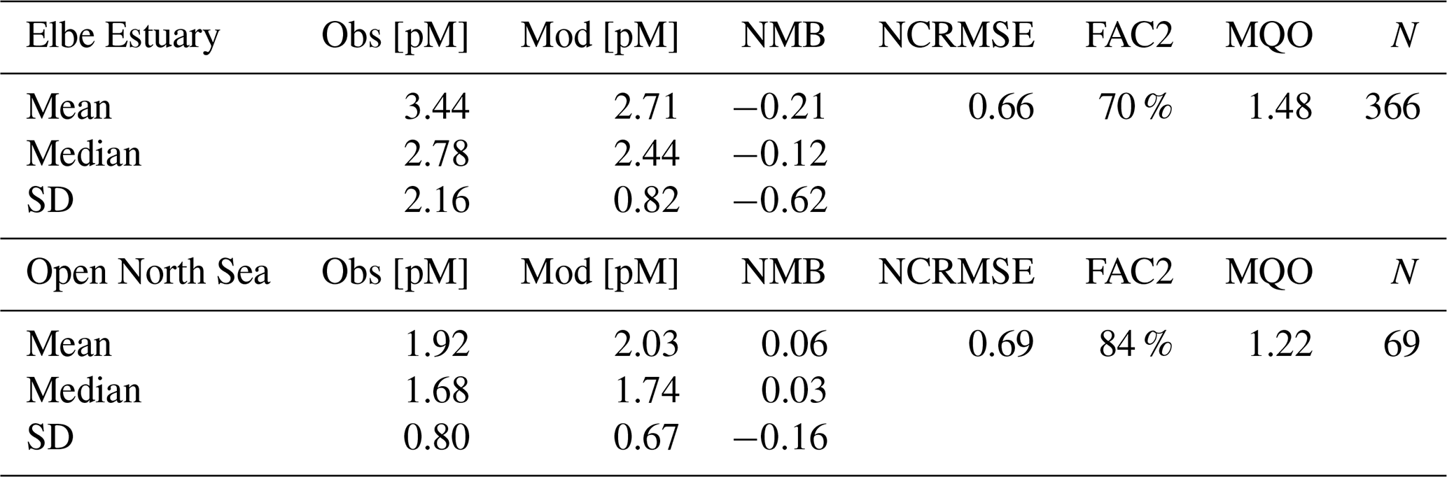
HgT concentrations in the North Sea do not exhibit a pronounced seasonality, and the observed variability is driven by a strong land–sea gradient along the European coastline where Hg from rivers is transported northeastwards from the English Channel by the Coriolis force (Fig. 7d). For the analysis, we split the North Sea Hg observations into two groups: (1) the Elbe Estuary (N=366) and (2) the open North Sea including a few observations near the remaining coastline (N=69). Due to the significant Hg inflow from the Elbe (1164 t a−1), Hg concentrations are higher in the Elbe Estuary with a mean concentration of 3.44 pM (Table 6). The model is able to reproduce the observed average (NMB %) but has a better agreement with the median values (−12 %). In this region, random and amplitude errors are dominant. This is indicative of subgrid dynamics and our inability to resolve the seasonality of Hg from rivers stemming from the use of static river loads for the entire run (OSPAR Commission et al., 2016). However, with 70 % of model values within a factor of 2 of the observations and an MQO of 1.48, the model is still close to our quality goal.
In the less dynamic open North Sea, the model performs better (FAC2 = 84 %, MQO = 1.22) (Table 6). The observed average of 1.92 pM is matched by the model (2.03 pM), and the bias is close to zero (NMB = 6 %). Nevertheless, due to the inhomogeneous distribution of observations, this value is not indicative of the actual background Hg concentrations in the open North Sea. We find that Hg concentrations there are mostly in the range of 1.1 to 1.5 pM.
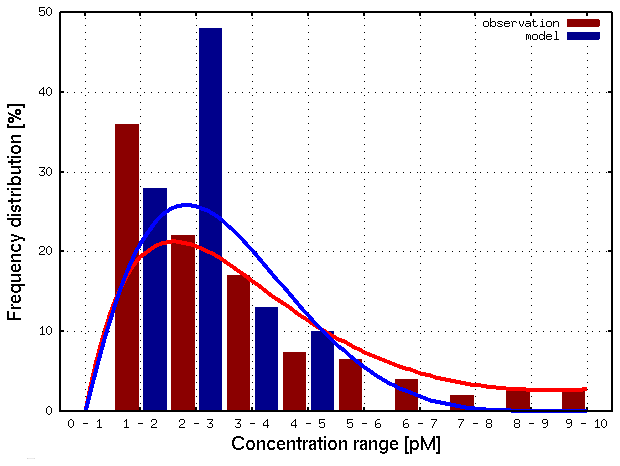
Figure 8Frequency distribution of observed (red) and model (blue) HgT. Concentrations for the North Sea (N=435).
In summary, for HgT, the model is close to our quality criterion (MQO ≤1.0). Improvements to the MQO could likely be achieved by increasing model resolution in the complex coastal regions and including more detailed input from rivers and particle resuspension at the European coastline. Especially for the Wadden Sea, a hydrodynamical model that can model the intertidal zone would be preferential.
Table 6Regional model performance for HgT in the North Sea. The evaluation is based on 435 measurements from the MARENET database (MARENET, 2020). Obs: observations; Mod: model.
3.4.2 Baltic Sea (HgT)
In the Baltic Sea, model performance for HgT is similar to in the North Sea (FAC2 = 70 %, MQO = 1.28) with a low bias (NMB = −19 %) and a high random error (NCRMSE = 102 %) (Table 7). Unlike for the North Sea, the model predicts a pronounced seasonality with surface HgT concentrations around 50 % higher during March (Fig. 9a) compared to August (Fig. 9b), which is in line with observations from Kuss et al. (2017) taken in March and July–August (Fig. 9). The two processes governing this are (1) stratification and particle settling in the central Baltic deep basins after the onset of primary production – this is the biological pump as POC particles here are mainly of biological origin (detritus) – and (2) increased photoreduction and subsequent atmospheric exchange of Hg0 (air–sea exchange). Additionally, during winter higher atmospheric Hg0 concentrations due to heating-related emissions and a shallow planetary boundary layer reduce and sometimes even reverse the Hg0 air–sea gradient. In the open Baltic Sea, Hg concentrations are mostly between 1.0 and 1.5 pM. In stratified areas, HgT concentrations can drop down to 0.5 pM during summer. During autumn and winter, mixing and upwelling can occasionally transport Hg from deeper waters upwards, sometimes leading to surface concentrations above 2 pM in some areas.
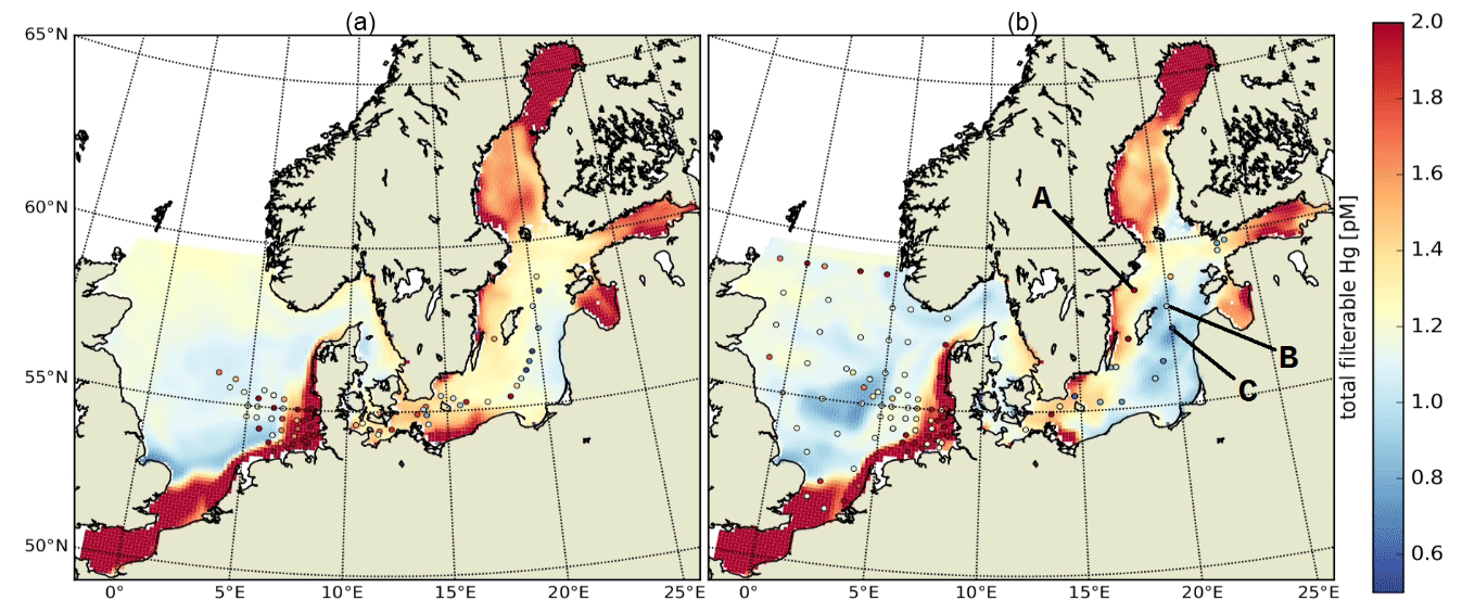
Figure 9HgT surface concentrations for (a) March and (b) August. Dots indicate observations (Kuss et al., 2017; Soerensen et al., 2018; MARENET, 2020).
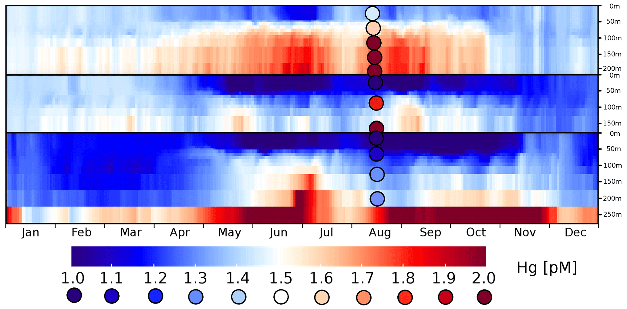
Figure 10Surface transect of the HgT concentrations in the Baltic Sea. The x axis gives 365 daily averages for the year 2010; the y axis represents a transect from the German coast in the western Baltic (y=0) to the mouth of the Bothnian Sea (y=87).
Table 7Spatially aggregated observed and modeled HgT concentrations in the Baltic Sea.
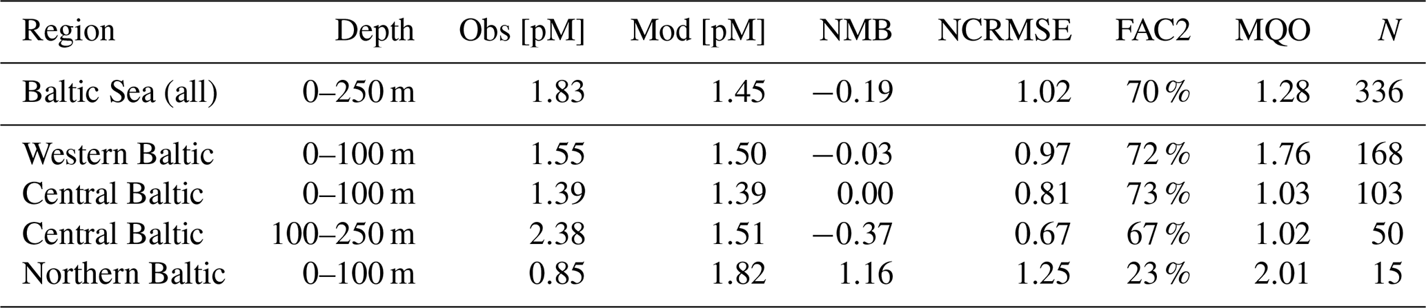
For a more detailed analysis, we separate the Baltic Sea into three regions: (1) the western part, which includes the Belt, Arkona, and Bornholm seas; (2) the Gotland Sea in the central Baltic; and (3) the northern part which includes the Bothnian Sea and Bothnian Bay. Moreover, we evaluate the oxic surface/intermediate waters and the deep anoxic waters in the Gotland area separately (Table 7). It is seen that the model is able to reproduce surface concentrations in the western and central areas with a bias close to zero. The model bias is larger in the deep basins, but model performance is still comparable to the North Sea. Here, the low vertical resolution in the model setup below 100 m will play a role. In the northern part, the model strongly overestimates HgT concentrations. This overestimation was also seen in the Soerensen et al. (2018) model. Northern Baltic rivers tend to be low in POC but rich in DOC compared to temperate rivers (McClelland et al., 2016; Soerensen et al., 2017), highlighting the importance of DOC flocculation at the point where river water encounters higher-salinity water for the settling and removal of Hg in Bothnian Bay estuaries, something that is currently not included in our model.
Figure 10 depicts the seasonality and Fig. 11 three vertical profiles in the Gotland Sea. It is seen how quickly Hg concentrations can change in this region and, depending on physical drivers, how different the seasonality of vertical mixing can be. At location A (Gotland Deep) Hg concentrations are around 1.5 pM for most of the year with a strong surface depletion (1 pM) during August and September. At location C, located at the opposite side of Gotland, the seasonality is reverse with the highest concentrations (1.2–1.4 pM) during August and September and much lower concentrations (0.9–1.1 pM) throughout the rest of the year.
In summary, our conclusion is similar to that of the North Sea, i.e., that better data on Hg inputs from rivers and a better resolution of the physical processes in the domain seem the most promising options for improving model performance. Especially in the Bothnian Bay, Hg cycling seems to be strongly influenced by terrestrial organic matter. In the central Baltic, we found that typically used kd values around log(kd) = 5.5 are not sufficient to reproduce the observed Hg depletion in the surface waters. Here, as described in Sect. 2.3.2, we use a kd based on Tesán Onrubia et al. (2020) which is an order of magnitude higher and leads to improved correlation to observations (Table 4). In addition, a higher vertical resolution is advised as vertical transport has proven to be an issue with the current model setup. Due to the low model resolution below 150 m, numerical diffusion leads to an overestimation of mixing in the deep basins. Finally, for further model evaluation, it would be useful to increase the seasonal coverage of observations in the area.
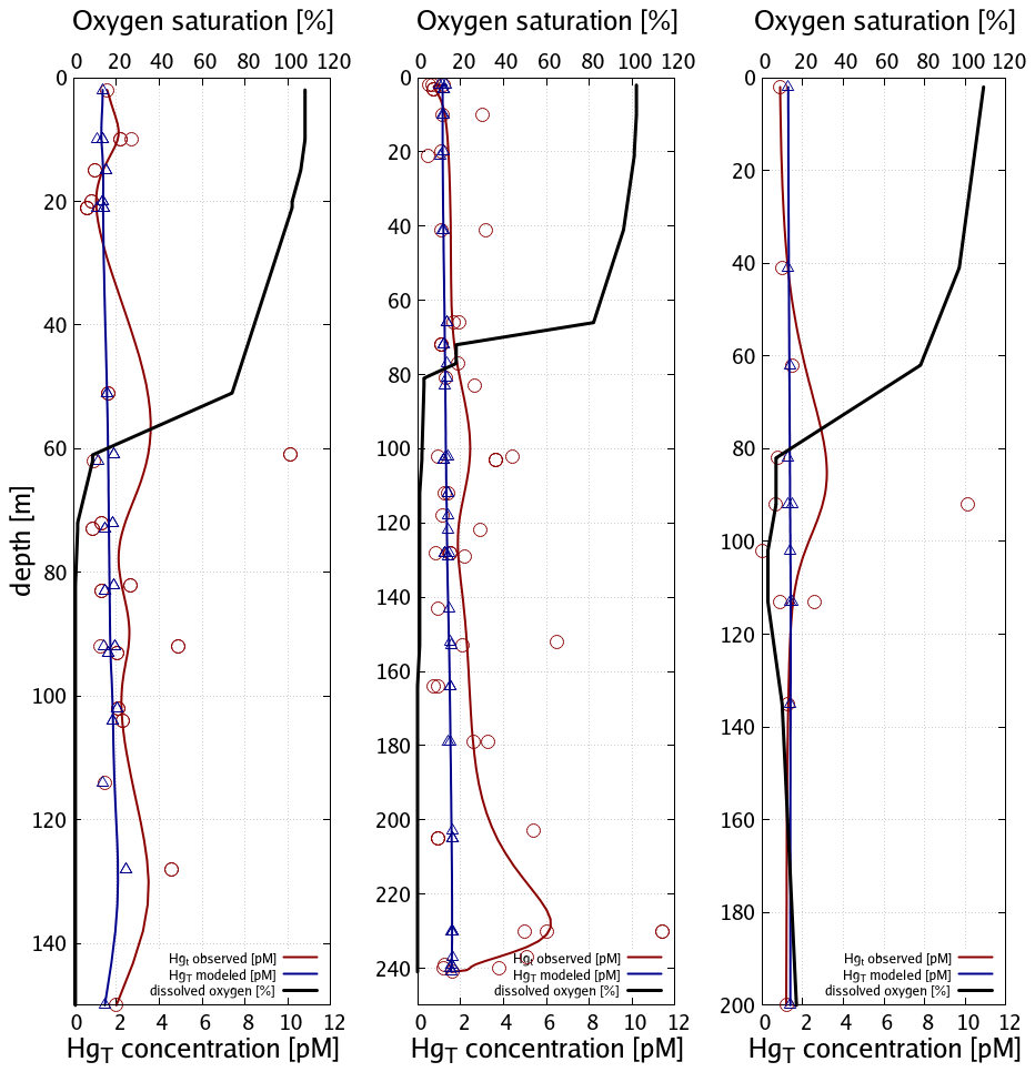
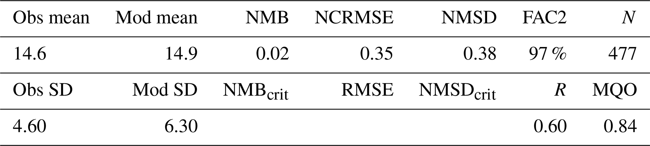
Figure 11Vertical Hg profiles in the central Baltic Sea observations (red) (Soerensen et al., 2018) and model values (blue) for the three central Baltic deep basins given in Fig. 9.
Finally, as the deep basins of the Baltic Sea are anoxic, in this area sulfur chemistry becomes relevant (Reactions R6–R9, Table 3). The effect of adding HgS and HgS–DOM to the chemistry scheme leads to particulate Hg–POM transforming into dissolved HgS species. The effect of this is two-fold: (1) firstly, Hg that is scavenged from the stratified surface layer by detritus (biological pump) accumulates directly at the boundary between oxic and anoxic waters. (2) Secondly, as eventually all inorganic Hg is transformed into HgS species, particle settling stops being a sink and Hg persists in the water column, whereas Hg is effectively transported to the sediment in model runs without sulfur chemistry. This leads to Hg concentrations being constant in the anoxic layer with higher values found only directly at the seafloor. Comparing to observations, we find that the model with sulfur chemistry is better able to capture the observed Hg distribution (Soerensen et al., 2018).
3.4.3 Elemental mercury (Hg0)
In the marine environment, elemental Hg0 makes up only a few percent of the total HgT. However, it is the species that determines the air–sea exchange and thus is a major driver for atmospheric long-range transport. With the oceans being the largest Hg emitter into the atmosphere (roughly twice as large as current anthropogenic emissions), marine Hg0 determines global transport patterns. Moreover, errors in modeled Hg0 concentrations propagate to all other Hg species and lead to wrong estimates for the compartmental budgets. Thus, it is of utmost importance to correctly reproduce Hg0 concentrations in surface waters. A detailed model study on Hg air–sea exchange in the North and Baltic seas has been published using a previous model version (Kuss, 2014; Kuss et al., 2018; Bieser and Schrum, 2016). The four main drivers of Hg0 concentrations are as follows:
-
the reducible fraction of Hg2+, which is typically estimated to be 40 % of the dissolved Hg;
-
the parameterization of biologically induced reduction processes;
-
the modeled photon flux and wavelength-dependent extinction in water impacting photolytic reduction;
-
air–sea exchange parameterizations, especially during high wind speeds.
Due to the fast exchange between atmosphere and water, Hg0 concentrations converge towards the equilibrium as described by Henry's law constant (Andersson et al., 2008). Therefore, in shelf seas a change in the redox chemistry directly affects the total HgT in the system. Due to the mixing in the coastal ocean, this impacts almost the complete waterbody. Moreover, the different reduction pathways produce a distinct seasonal pattern with Hg0 concentrations ranging from as low as 5 pg L−1 during winter to up to peaks >60 pg L−1 during cyanobacteria blooms. Thus because of the high intra-annual variability, the model needs to be evaluated against Hg0 observations throughout the year, as good agreement for a single cruise does not imply good model performance throughout the year.

Figure 12Comparison of modeled and observed Hg0 concentrations in surface waters for four cruises in the Baltic Sea (x axis: observations; y axis: model values) (Kuss, 2014; Kuss et al., 2018).
Table 8Comparison of modeled and observed Hg0 concentrations for four cruises in the Baltic Sea in 2006 (Kuss, 2014; Kuss et al., 2018).
The observed annual average Hg0 concentration for 580 measurements is 14.6 pg L−1; the modeled value is 14.9 pg L−1 with a systematic error of 2 % and a random error of 35 %. The random error is largest in summer (NCRMSE = 42 %) and is due to the biogenic reduction which depends on cyanobacteria biomass. The model shows good correlation with observations (R=0.60) and is able to reproduce the observed variability (NMSD = 38 %) (Table 8). All statistical metrics for Hg0 are well inside model performance criteria, and 97 % of the model values are within a factor of 2 of the observations. The model quality objective is below 1.0 (MQO = 0.84). Thus, the model performance is, at least for the given model resolution, in the range where further improvements are hardly feasible (Carnevale et al., 2014; Schutgens et al., 2016).
We acknowledge that the redox chemistry used is based on measurements in the Baltic Sea (Kuss et al., 2015). Thus, it needs to be investigated whether it shows equally good performance for other marine regions. We find that the model performs similarly well throughout the year with the largest bias during summer, when the dynamics driving biological and photolytic reduction lead to a higher variability in Hg0 concentrations (Table 9).
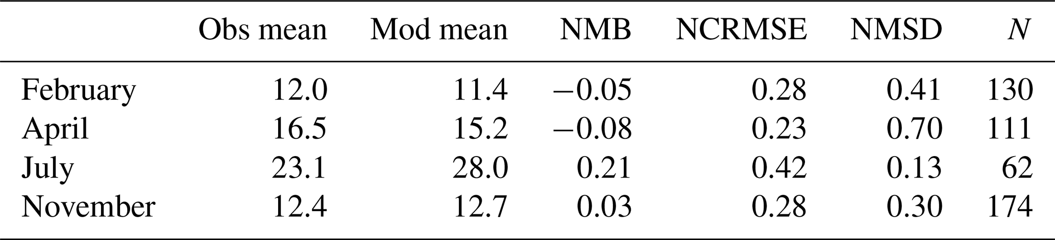
Figure 13 depicts the seasonality of a mean Hg0 for the Baltic Sea. Moreover, the contributions of the four reduction reactions (1) chemical reduction, (2) photolytic reduction, (3) biogenic reduction, and (4) reductive methylation (Table 3) are given. We find that the dark reduction is the dominant process, producing 55 % of the total Hg0 in the Baltic Sea and 70 % in the North Sea. Photolytic reduction contributes 34 % and biogenic reduction contributes 12 % annually. However, from July to mid-August the photolytic reduction becomes dominant (>50 %). When the cyanobacteria bloom starts, light penetration reduces significantly due to the increased marine particle load, and until the end of November the biogenic reduction becomes the dominant process (Fig. 13a). In contrast, as there are no cyanobacteria in the North Sea, photolytic reduction is dominant throughout the summer (Fig. 13b). The reductive methylation reaction plays a negligible role for Hg0 surface concentrations but can be a source for Hg0 in deeper waters with a high MeHg fraction. It can be seen that there is a background Hg0 concentration of about 5 to 15 pg L−1 due to the chemical (dark) reduction process. During model development, we recognized a systematic error in the seasonality (overestimation during summer and underestimation during winter) that could be resolved by introducing a temperature dependency of the chemical reduction reaction, a process which was detectable in the observations by Kuss et al. (2015) (Eq. 8, Sect. 2.3.1). For the photolytic reaction, we found that it is important to validate the radiation fields. Testing the model using different radiation fields resulted in a change in the annual net Hg0 production of >10 %. The main driver here is cloud coverage, which is a particularly uncertain state variable in meteorological models. Moreover, we want to note that photolysis rates from observations and incubation experiments are solely reported based on the photolytically active radiation. Due to the highly wavelength-selective light extinction it would be favorable to parameterize photolysis using the actual wavelengths absorbed by Hg. Finally, the biogenic reduction term in the model is driven only by the concentration of cyanobacteria. This creates the observed late-summer–early-autumn Hg0 peak. Allowing other phytoplankton species in the model to reduce Hg2+, leading to unrealistically high concentrations during the spring flagellate bloom.
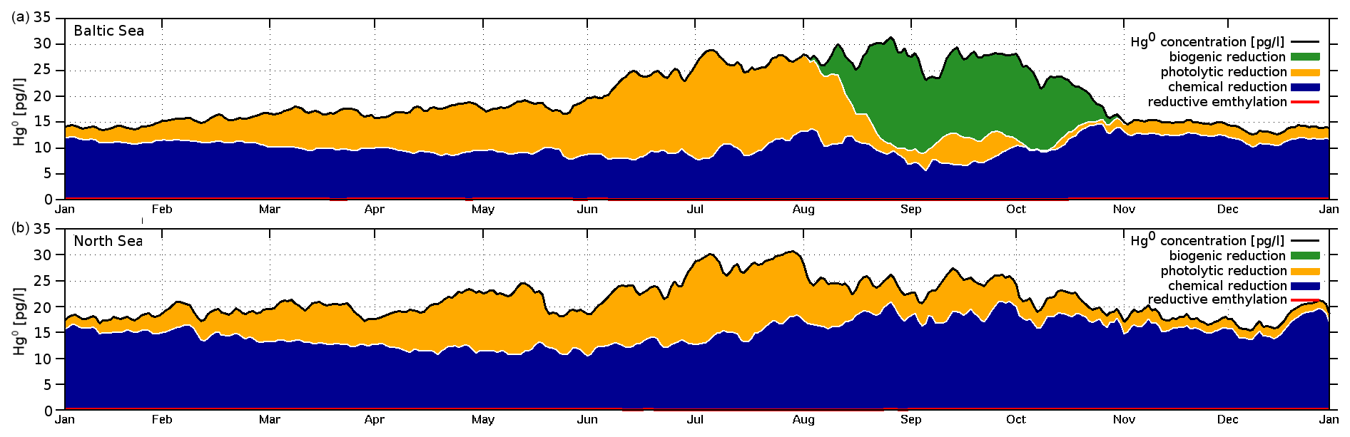
Figure 13Annual profile of mean Hg0 concentration in the Baltic Sea (a) and North Sea (b). The colored areas indicate the contribution of individual reduction pathways (Reactions R1, R3, R20; Table 3).
3.4.4 Methylmercury (MMHg+ and DMHg)
Due to the complexity of the analytical methods and the extremely low environmental levels of observed concentrations, MeHg observations in the marine environment are rare. Additionally, they are the most uncertain observations. Here, to calculate the MQO, we assume an uncertainty of 50 %. We evaluate the model predictive capabilities in reproducing (1) MeHg concentrations and (2) the methylated Hg fraction Mfrac= MeHg HgT. The latter allows us to evaluate the modeled net methylation independently of the HgT model error (Table 10). In the Baltic Sea, observed MeHg concentrations are in the range of 191 (20–603) fM, while the modeled range is 213 (57–350) fM. For Mfrac the observed range is 11.4 % (1.3 %–30.4 %) (10th and 90th percentiles), while the model predicts 9.9 % (3.6 %–20.2 %). The frequency distribution for observed and modeled Mfrac is given in Fig. 15. The model is in very good agreement with the observations on average but cannot reproduce the observed extreme values. In total there are 17 (6.5 %) samples with a Mfrac between 33 % and 73 %, all of which were measured in the intermediate layer between 70 and 160 m.
Evaluating the relative Mfrac metric instead of absolute MeHg concentrations reduces the systematic error from −28 % to 5 % and the amplitude error from −74 % to −55 %. This shows that the HgT bias accounts for roughly 80 % of the MeHg systematic error and 50 % of the amplitude error. Yet, using Mfrac has no significant effect on the random error, indicating a non-linear relationship between the methylated fraction and the absolute amount of MeHg. While systematic error and amplitude error are comparable to the other Hg species, the random error is much larger (NCRMSE = 1.9). This shows that the methylation–demethylation dynamics in the model are too simplified, pointing to missing processes in the model. Figure 15 depicts MeHg and Mfrac vertical profiles for the central Baltic Sea deep basins in different years and seasons together with oxygen concentrations. Again, it can be seen that the model is able to reproduce the average vertical profiles but is incapable of capturing the high and low values. Observations indicate an MeHg hotspot near the oxycline. Here, Mfrac can become as large as 100 %, meaning that almost all mercury there is present as MeHg. The highest MeHg observations coincide with anoxic conditions, indicating that the availability of dissolved HgS drives methylation in these regions (Soerensen et al., 2018). In Fig. 15, anoxic regions are indicated by negative oxygen concentrations. These are based on measurements of H2S, and the net oxygen is calculated based on the reaction H2S + 2O2→ H2SO4.
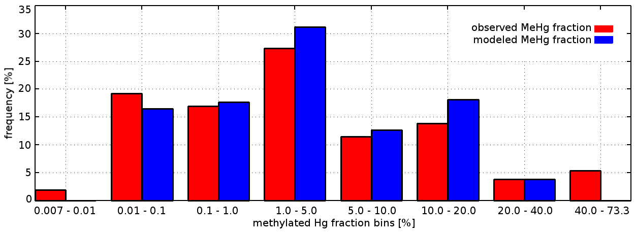
Figure 14Observed (Kuss et al., 2017; Soerensen et al., 2018) and modeled frequency distribution of the methylated Hg fraction Mfrac.
Table 10Evaluation of seasonally and vertically clustered Mfrac observations against model values.
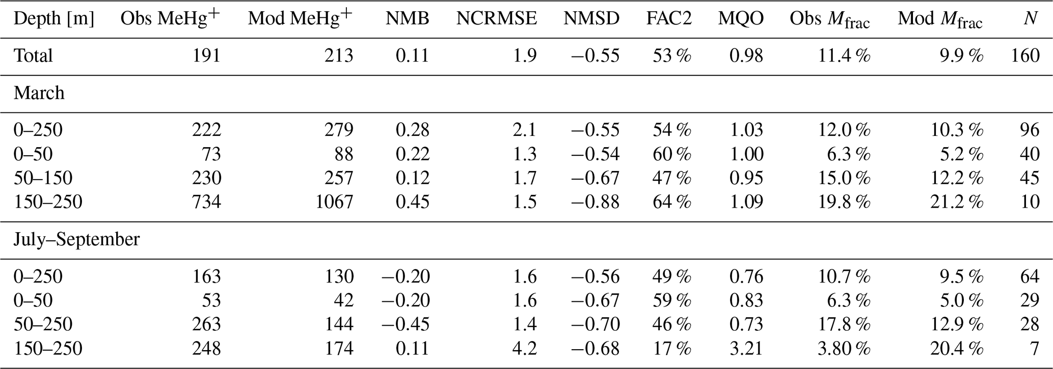
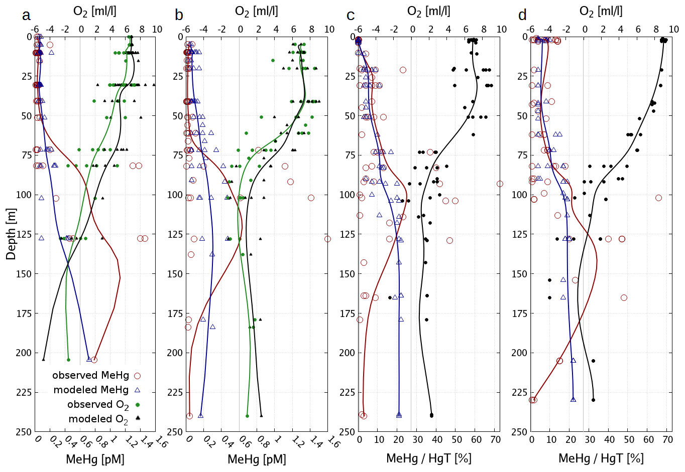
Figure 15Vertical MeHg profiles for Baltic deep basins. Negative oxygen concentrations indicate sulfide concentrations. (a) MeHg profiles 2014 (Soerensen et al., 2018); (b) MeHg profiles 2015 (Soerensen et al., 2018); (c) Mfrac March (Kuss et al., 2017); (d) Mfrac July–August (Kuss et al., 2017).
The model can reproduce the seasonality and vertical gradient of the methylated fraction. On the one hand photolytic demethylation leads to lower MeHg concentrations in the surface ocean during summer. On the other hand, biological activity leads to increased MeHg formation in spring and summer. We find that a biologically induced methylation parameterized with biomass or phytoplankton concentration leads to spring becoming the season with the most effective net methylation. By linking biological methylation to the remineralization of organic carbon, we introduce a temperature dependency that shifts this towards summer (Fig. 16) (Eq. 9, Sect. 2.3.1). Yet, the model still overestimates methylation in spring and underestimates methylation in summer. For a more detailed analysis, we look at surface layer MeHg concentrations on four specific dates. Figure 17 depicts MeHg measurements for 21 March and 1 August of the years 2014 and 2015. In March MeHg concentrations are between 40 and 300 fM and in August between 10 and 200 fM with pronounced spatial gradients. This “spottiness” of the MeHg concentrations partially explains the large random error in the model. Moreover, while the general patterns are similar, methylation shows a significant interannual variability (Fig. 17).
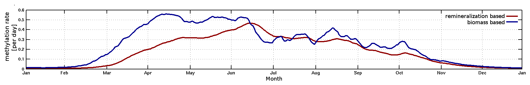
Figure 16Seasonality of the biologically induced methylation reaction using different parameterizations (Reaction R12, Table 2).
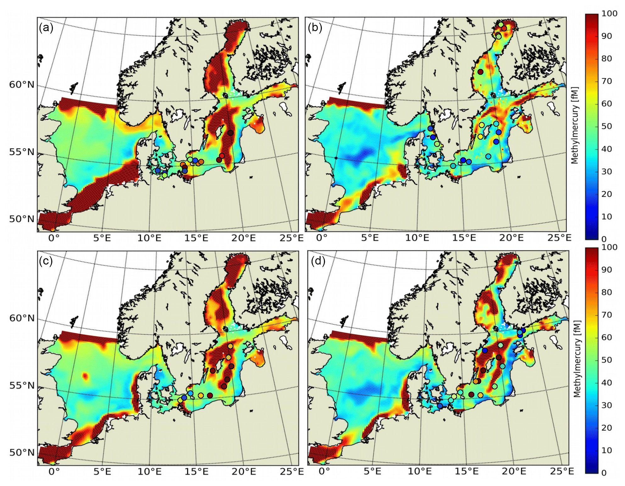
Figure 17Methylmercury concentrations in the surface ocean on (a) 21 March 2014, (b) 1 August 2014, (c) 21 March 2015, and (d) 1 August 2015. Superimposed are all observations at depths of 0–50 m (Table 9).
Overall, the model reproduces 53 % of MeHg values within a factor of 2. We find that the model performance (MQO = 0.98) is still within the quality criterion. This is due to the much higher uncertainty in MeHg measurements, for which we assumed an error of 50 %. This indicates that further model improvement will be difficult unless more frequent and more precise MeHg measurements become available. Moreover, to reach their full potential MeHg observations need to be combined with extensive auxiliary data. This starts with simple parameters like incoming solar radiation to determine the actual intensity of photolysis or better estimates for special partitioning coefficients for MeHg. In our model, for example, we use a lower kd of MMHg+ compared to Hg2+, which means that particle settling will increase Mfrac with increasing depth (Table 4, Sect. 3.2.3). Moreover, chemical parameters such as O2 and H2S concentrations have been shown to impact the availability of inorganic Hg2+ species for methylation. And finally, microbiological observations ranging from chlorophyll concentration to RNA show the activity of methylating bacteria could improve variable methylation rates. From our model evaluation, it seems clear that fixed methylation and demethylation rates cannot account for the observed variability in both MeHg concentrations and the methylated Hg fraction Mfrac. Here, we need a better understanding of the parameters modulating methylation and demethylation rates.
3.4.5 Hg in biota
Figure 18 depicts annual average Hg loads in the different ecosystem biota species. The North Sea exhibits higher Hg loads in biota, which can be explained by the high Hg load from rivers, especially the Elbe and Scheldt; the lack of permanent sedimentation; and the earlier onset and higher overall primary production, which increases the effectiveness of the active uptake pathway. The average amount of Hg in biota ranges from 1 % to 5 % of the HgT with higher values in the highly productive North Sea. During winter only a little Hg is bound in biota due to the low biomass, while in summer the fraction can be up to 10 %. Due to the high transfer efficiency of MMHg+ (97 %), on average, between 5 % and 20 % of the total MMHg+ is accumulated in biota. In highly productive regions the amount of MMHg+ inside biota can even be larger than the MMHg+ remaining in the water column. Flagellates (Fig. 18b) are the most abundant phytoplankton species and thus the most important primary accumulator. However, the diatom bloom occurs earlier in the year and removes MeHg from the water column before the flagellate bloom. The higher Hg load in diatoms (Fig. 18a) is due to their lower carbon content. Finally, cyanobacteria (Fig. 18c), which can lead to major blooms in late summer–early autumn, are the dominant species later in the year, and MeHg loads during the bloom exceed those of the diatoms and flagellates. Due to the active Hg uptake, micro- (Fig. 18d) and mesozooplankton (Fig. 18e) have a higher accumulation factor than the phytoplankton species. Finally, Fig. 18f depicts the Hg load in fish.

Figure 18Annual average HgT concentrations [ng L−1] in biota: (a) diatoms, (b) flagellates, (c) cyanobacteria, (d) microzooplankton, (e) mesozooplankton, and (f) fraction of Hg in fish.
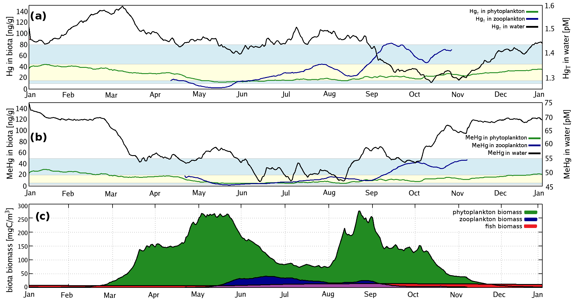
Figure 19Seasonality of modeled (a) Hg and (b) MeHg loads in phytoplankton and zooplankton. Superimposed is the water concentration of (a) Hg and (b) MeHg. Panel (c) gives the integrated biomass. All values are averages for the Baltic Sea integrated over the top 100 m.
As the last step of the model evaluation, we compare HgT and MeHg loads in biota to observations. Field studies investigating the total Hg content of biota are fairly common and can be used to estimate the model bias. However, only few data on MeHg in biota and species diversity are available. On average the observed HgT content in phytoplankton lies in the range of 0.002±0.001 µg g−1 wet weight and that for zooplankton in the range of 0.006±0.005 µg g−1 wet weight (Nfon et al., 2009). Here, we use a conversion factor for wet weight (w.w.) to dry weight (d.w.) of 0.2 for phytoplankton and 0.16 for zooplankton (Cushing, 1958; Ricciardi and Bourget, 1998). Moreover, biomass in ECOSMO is defined in milligrams of carbon, whereas observations are reported in milligrams w.w. or milligrams d.w. We estimate the ratio of milligrams of carbon to milligrams d.w. as 0.2 for diatoms, 0.33 for flagellates and cyanobacteria, and 0.5 for zooplankton (Sicko-Goad et al., 1984; Walve and Larsson, 1999). With this, we estimate the expected average HgT loads in biota in the Baltic Sea in the range of 30 (15–45) ng g−1 C in phytoplankton and 75 (10–120) ng g−1 C in zooplankton. MeHg loads in phytoplankton are expected to be around 10 (5–15) ng g−1 d.w., while they are larger for cells with a larger surface-to-volume ratio (Pickhardt and Fisher, 2007; Soerensen et al., 2016b). Figure 19 depicts the average HgT and MeHg loads in phytoplankton and zooplankton. For phytoplankton, the model lies well within the expected range for HgT (25–80 ng g−1 C) (Fig. 19a) and MeHg (5–15 ng g−1 C) (Fig. 19b). During winter when phytoplankton biomass is low (Fig. 19c), Hg loads reach the maximum of the expected bioaccumulation range, and once production starts, growth dilution lowers the modeled HgT and MeHg loads and their concentrations in the water column decline by 10 % and 20 % respectively. For zooplankton, values are well within the expected range. They start low at the beginning and rise over the year. At the end of the year, cyanobacteria start to dominate the phytoplankton community, leading to higher phytoplankton MeHg concentrations and another decline in marine HgT concentrations. At the same time, the decrease in diatom and flagellate concentration leads to an increase in the fraction of microzooplankton of the mesozooplankton diet, increasing their trophic level and further increasing the zooplankton HgT load. Finally, with Hg loads between 70 and 140 ng g−1 C d.w., fish are the highest trophic level in the ecosystem model. Due to the much more efficient active uptake of MMHg+ compared to Hg2+ in fish, 60 % to 80 % of the accumulated Hg is in the form of MMHg+. Looking at the two uptake pathways of bioconcentration and biomagnification, we find that biomagnification is responsible for 80 % to 90 % of the total Hg uptake for non-phytoplankton species. A more detailed analysis can be found in Amptmeijer et al. (2023).
Next, we evaluate the model capabilities to reproduce Hg content in fish. For this, we compare the modeled bioaccumulation in the functional ecosystem group representing fish to herring. This pelagic species corresponds best to the fish functional group implemented into ECOSMO (Daewel et al., 2019). The analysis is based on 1166 measurements of Hg in fish muscle tissue. We use the same conversion factors as for zooplankton to convert the model carbon dry weight to wet weight total biomass (1 ng g−1 C d.w. = 3.125 ng g−1 w.w.). For this, the dataset is split into five Baltic Sea regions:
-
the Swedish west coast, a stripe from Gothenburg to Oslo;
-
the southern Baltic Proper, which includes the Bornholm Sea and the southern Gotland Sea;
-
the northern Baltic Proper, which includes most of the Gotland Sea;
-
the Bothnian Sea;
-
the Bothnian Bay.
It is not possible to compare the caught fish to an individual model grid cell and time step. Therefore, we compare them to observed average HgFish concentrations. The model reproduces the observed average HgFish of 28 ng g−1 in the Baltic Sea with a systematic error of −9 % (HgFish=25 ng g−1) (Table 11). In order to estimate the model variability in HgFish for each region, we vertically integrate annual average model values for each grid column. The result is a fish dataset in which each member represents a model fish that has spent its life in a single 10×10 km2 water column. In reality, herring are not confined to 10×10 km2 grid cells, and their Hg accumulation depends on their migration patterns. Yet, we argue that this approach approximates the model spread (Fig. 20). This allows us not only to calculate the bias but also to estimate the model standard deviation. On average, over the whole Baltic Sea, the model captures the observed variability (NMSD = 9 %). The error is driven by the west coast region (NMSD = 309 %), while it varies between (29 %–76 %) in the remaining Baltic Sea. In the west coast region, the observed fish exhibit less than half the variability observed in all other regions. While the model captures the variability in the other regions, it shows the opposite behavior to the observations on the west coast. In this shallow region, we explain the high model concentrations by regular Hg resuspension from sediments, which creates pockets of elevated HgT and MeHg concentrations. Thus, the large model spread is an artifact of our methodology based on static fish.
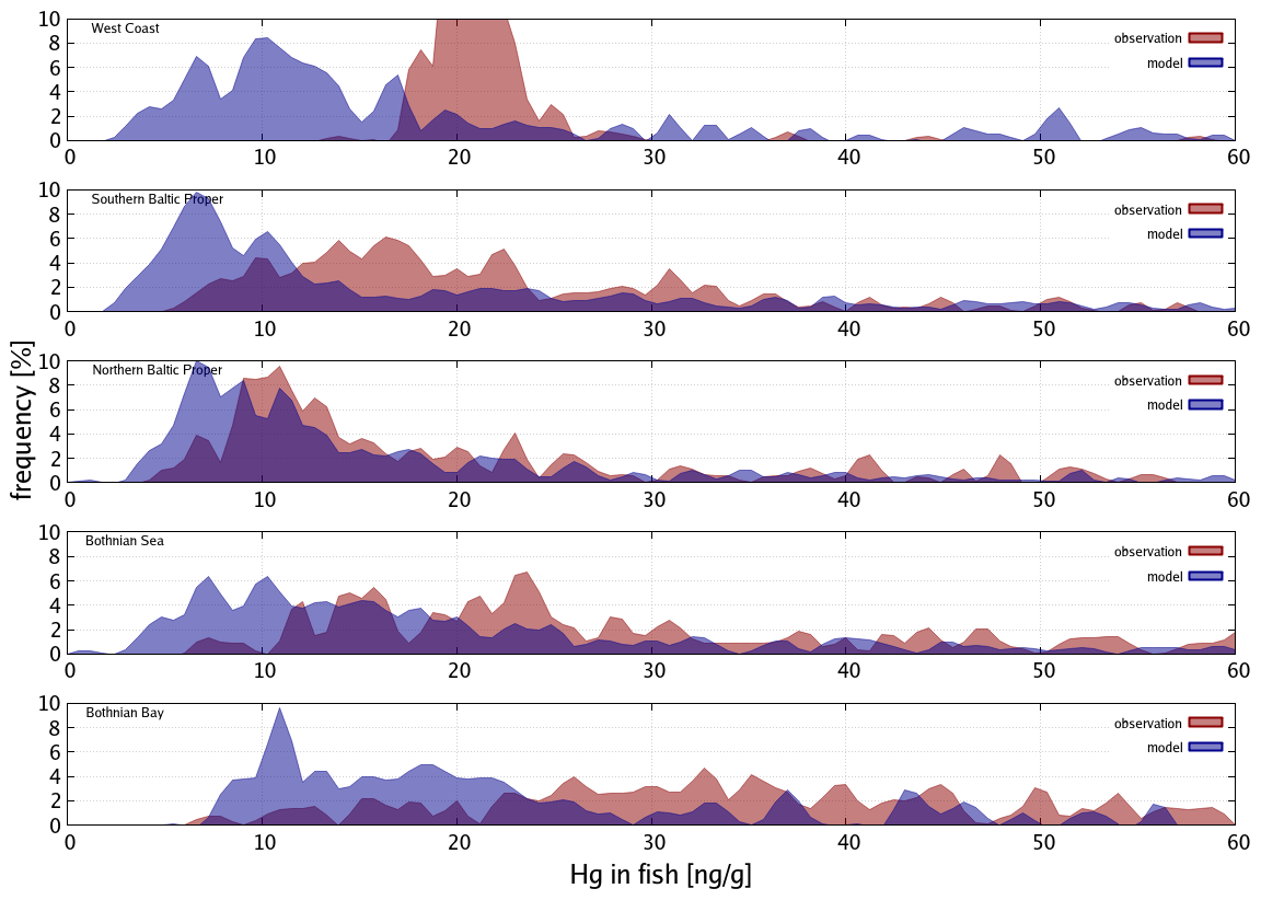
Figure 20Modeled and observed frequency distribution of Hg in fish in the Baltic Sea regions (Soerensen and Faxneld, 2020).
In this paper, we present the regional-scale 3D high-resolution biogeochemical multi-media Hg model MERCY v2.0. The numerical model combines hydrodynamic models for the atmosphere and ocean, including a marine ecosystem model. MERCY includes a comprehensive marine Hg scheme to calculate transport, transformation, and bioaccumulation. The schemes for chemistry, partitioning, and bioaccumulation are based on literature values, and no domain-specific model tuning has been done. We would like to emphasize that MERCY is suitable for any marine region or even for global application. The major factors when applying the MERCY model to other regions are (1) partitioning coefficients to organic material (OM) as the type of OM varies regionally; (2) the parameterization for biogenic reduction as the values presented here are based on cyanobacteria in the Baltic Sea; and (3) the ecosystem model, as trophic dynamics and phytoplankton uptake rates can vary widely between regions. To our knowledge, it is the first model capable of linking atmospheric Hg emissions to MeHg accumulation at higher trophic levels. The intention of this initial model publication is the detailed presentation of the model and first results, focusing on model performance evaluation and the identification of the processes and parameters responsible for the model error. A more comprehensive analysis of the dynamics of and variability in Hg speciation, partitioning, and bioaccumulation is required for future studies. While our model performs more realistically than earlier models for marine Hg cycling, there are still large uncertainties, especially regarding methylation.
Table 11Model performance evaluation of HgT, dissolved elemental Hg0, and the methylated Hg fraction. The model error is separated into systematic error (normalized bias), random error (normalized centered root-mean-square error), and amplitude error (normalized mean standard deviation). The model quality objective target value is MQO <1.0 (consult Sect. 3.1 for more information).
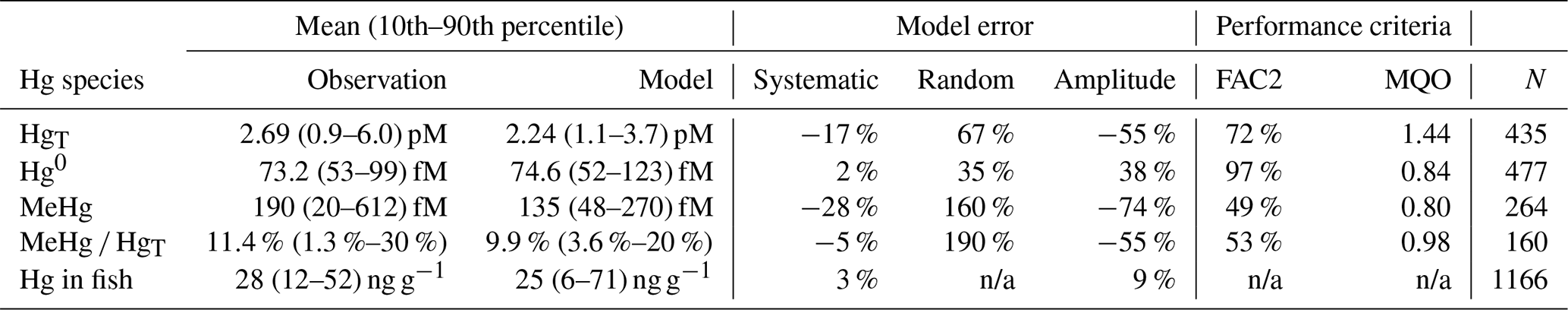
n/a: not applicable.
We evaluated model performance for key Hg species based on a simulation for the North and Baltic seas for the years 2000 to 2016. We chose these regions due to the availability of observations. Moreover, the two regions cover a range of regimes, have high primary productivity, and are relevant to fisheries. Unlike atmospheric Hg modeling, there is no precedent or scientific consensus defining the state-of-the-art requirements and limitations of reproducing concentrations of different marine Hg species. Considering the inherent uncertainty in a comparison of model values and observed concentrations (e.g., measurement error, sampling error, error in the hydrodynamic models, the uncertainty in reaction rates, and unknown processes), we define model values within a factor of 2 of the observations as a reasonable agreement. Moreover, we used a statistical model quality objective (MQO <1.0) to assess the model skill (Carnevale et al., 2014) (Sect. 3.1).
A detailed model performance evaluation for the North and Baltic seas demonstrates that the model can reproduce concentrations and seasonality of single Hg species to a degree that validates the model predictive capabilities. For HgT, the model is able to reproduce 72 % of the observations within a factor of 2 (Table 12). We find that the model can reproduce background concentrations in the open parts of the shelf seas (1.0–1.5 pM). The model error can mostly be attributed to random and amplitude error. The main source of uncertainty in the model is the transport dynamics of the large Hg influx from rivers and the Wadden Sea. These lead to observed Hg peaks of up to 10 pM. The model resolution of 10×10 km proved insufficient to reproduce the observed temporal and spatial gradients. Because the majority of observations are at the coast near major rivers, the model does not reach the quality objective (MQO = 1.44). Moreover, in the Baltic Sea, the model overestimates vertical mixing from deeper regions with elevated Hg concentrations. This is caused by the coarse vertical resolution below 150 m, which leads to numerical diffusion and an underestimation of stratification. We found that including sulfur chemistry improves model performance in the deep anoxic water layer in the Baltic Sea basins. The mechanism is that Hg transported downwards from the stratified oxic and productive surface layer through the biological pump transforms into dissolved HgS species in anoxic waters. This stops the downward gradient and lessens the role of the sediments in this region as a sink.
We summarize that the improvement of the model performance for HgT requires optimizing of the hydrodynamic model. Unless circulation patterns, stratification seasonality, resuspension events, and upwelling regions are correctly represented, hardly any improvement of the model can be achieved. Further, for the coastal ocean, we find that river inflow needs to be better resolved, ideally with daily loads including fluxes of dissolved and particulate carbon. Finally, particle partitioning and subsequent sedimentation comprise a major source of uncertainty. We achieved better results using a log(kd) of 6.6 (Tesán Onrubia et al., 2020), which is an order of magnitude higher than those used by other models.
The model performed best for elemental Hg0. Due to air–sea exchange, Hg0 is the key species controlling the exchange between the atmosphere and ocean. Any bias in modeled Hg0 fields directly influences the marine total Hg budget and leads to unrealistic results. MERCY is able to reproduce 97 % of Hg0 measurements within a factor of 2. We find that the chemical (often referred to as dark) and photolytic reduction processes produce roughly the same amount of Hg0 annually although with different seasonality. Moreover, elevated Hg0 concentrations in the Baltic Sea between July and October could be reproduced by implementing biological reduction by cyanobacteria. Finally, we find that it is important to consider temperature dependence for the chemical reduction reaction to correctly reproduce the seasonality. With a model skill of MQO = 0.84, we conclude that the model performance for Hg0 is in a range where further improvements become marginal. Possible improvements are photolytic reaction rates based on actual wavelengths instead of the photolytic active radiation and a better understanding of biological reducers.
Evaluation of MeHg resulted in the methylated fraction Mfrac (MeHg HgT) for which 55 % of model values are within a factor of 2 of observations. The model is able to reproduce the observed mean and seasonality but is unable to capture the observed maxima, resulting in a large random error. Yet, because of the high measurement uncertainty, the model still reaches the quality objective (MQO = 0.98), indicating that the observations are limiting model development. We found that producing realistic MeHg concentrations throughout the year required methylation occurring in oxic waters. Oxic methylation is the primary or sole source (80 %–100 %) of MeHg in large parts of the model domain. The anoxic methylation reaction is dominant in anoxic waters (the deep basins of the Baltic Sea). We found that assumptions made in other models linking methylation to productivity or chlorophyll concentrations pose two problems: firstly, they lead to regions with zero MeHg in seasons with no primary production and very low MeHg concentrations in the deep anoxic basins. And secondly, they produce a phase error in the seasonality due to an overestimation of MeHg during the spring bloom. In MERCY, we parameterize the biogenic methylation with the amount of remineralized organic matter, which adds a temperature dependence to the process that in turn reduces the impact of the spring bloom. Moreover, various sensitivity runs using varying parameters to modulate the biogenic methylation rate to test for possible biological drivers have failed to surpass model formulations including a constant oxic methylation reaction. We summarize that poor model performance for MeHg is the key source of uncertainty in the presented model. In order to improve the model performance, a more detailed understanding of methylation processes is required. Moreover, more high-quality observations, especially on MeHg seasonality, are needed to allow for model-based process studies. The addition of isotopic fractionation to the model might also help to further constrain sources and sinks of MeHg.
Finally, we evaluate the model's ability to reproduce Hg in biota. Our model provides Hg and MeHg loads in phytoplankton, zooplankton, and fish which are inside of the observed range. We find that the modeled phytoplankton concentrations vary within the observed maximum and minimum loads. Zooplankton changes at the trophic level over the course of the year due to changes in diet. As expected, the model predicts the highest MeHg loads in fish, making up 90 % of the total Hg in fish due to its high transfer efficiency. Most parameters used for bioaccumulation are highly uncertain, and there is ample room for improvement in this part of the model. We hypothesize that the ecosystem model which is focused on correctly reproducing carbon fluxes, needs improvements regarding functional traits relevant to bioaccumulation such as size, shape, or feeding behavior.
The presented model allows hypothesis testing within a consistent physical–biological–biogeochemical framework based on basic principles. We are currently working on a model version that allows for seamless coupling with different hydrodynamic ocean and marine ecosystem models to increase the applicability of the model. The model performance is here only cursorily evaluated to limit the length of the paper. For the future, we plan to investigate the sources of model uncertainty and sensitivity in order to identify the insufficient understanding of the processes and find out the imprecise or unknown parameters, especially concerning methylation and biological uptake. Finally, we want to employ and promote the MERCY model as a tool for hypothesis testing and prediction within a consistent physical–biological–biogeochemical framework based on basic principles. This will enable researchers to (1) improve our understanding of the natural variability from seasonal to decadal timescales; (2) investigate forcing dynamics, leading to MeHg accumulation in seafood; and (3) estimate the impact of anthropogenic and natural drivers in support of the Minamata Convention on mercury.
The MERCY v2.0 source code is freely available at https://doi.org/10.5281/zenodo.7101217 (Bieser, 2022).
COSMO-CLM v4.0 is freely available at https://doi.org/10.5281/zenodo.5939757 (Rockel, 2022).
CMAQ v4.7.1 is an active open-source development project of the US Environmental Protection Agency (EPA) that consists of a suite of programs for conducting air quality model simulations. The model is freely available at https://doi.org/10.5281/zenodo.1079879 (US EPA Office of Research and Development, 2010).
HAMSOM-ECOSMO_2e2 v1.0 is freely available at https://doi.org/10.5281/zenodo.7587005 (Daewel, 2023).
The code is also available from the Helmholtz Centre Hereon Git repository: https://coastgit.hzg.de/udaewel/hamsom-ecosmoe2e/ (last access: 1 March 2023).
The data used in this article are available as follows:
-
ERA-Interim (https://apps.ecmwf.int/datasets/data/interim-full-daily, last access: 7 April 2023; Herbach et al., 2020);
-
GEBCO 2022 gridded bathymetry (https://doi.org/10.5285/e0f0bb80-ab44-2739-e053-6c86abc0289c; GEBCO Compilation Group, 2022);
-
Mercury observations in water and sediments of the North and Baltic seas – MARENET (https://www.bsh.de/DE/DATEN/Klimaund-Meer/Meeresumweltmessnetz/messnetz-marnet_node.html, last access: 7 April 2023; Hohlfeld and Wolff, 2015);
-
Mercury observations in fish (https://www.sgu.se/produkter-och-tjanster/nationella-datavardskap/datavardskap-for-miljogifter/biota/, last access: 1 March 2023; Soerensen and Faxneld, 2020).
The authors contributed as follows.
| Contributor role | Role definition | Authors |
|---|---|---|
| Conceptualization | Ideas and formulation or evolution of overarching research goals and aims | |
| – for the mercury model | JB | |
| – for the bioaccumulation model | DA, UD, JB | |
| Methodology | Development or design of methodology and creation of models | |
| – Hg chemical mechanism | JB, JK, ALS | |
| – Hg and MeHg bioaccumulation | DA, JB | |
| Software | Programming and software development, designing computer programs, implementation of the computer code and supporting algorithms, and testing of existing code components | |
| – for HAMSOM and ECOSMO | UD | |
| – for MERCY | JB | |
| Validation | Verification, whether as a part of the activity or separate, of the overall replication/reproducibility of results/experiments and other research outputs | JB |
| Formal analysis | Application of statistical, mathematical, computational, or other formal techniques to analyze or synthesize study data | |
| – for HgT and MeHg concentrations | JB | |
| – for Hg0 concentrations and air–sea exchange | JB, JK | |
| – for Hg and MeHg bioaccumulation at lower and higher trophic levels | DA, ALS | |
| Investigation | Conducting a research and investigation process, specifically performing the experiments, or data/evidence collection | JB, JK, ALS |
| Resources | – Provision of study materials, reagents, materials, patients, laboratory samples, animals, instrumentation, computing resources, or other analysis tools | CS |
| – Hg and MeHg observational data | JK, ALS | |
| Data curation | Management activities to annotate (produce metadata), scrub data, and maintain research data (including software code, where it is necessary for interpreting the data themselves) for initial use and later reuse | ALS, JK, UD |
| Writing – original draft preparation | Creation and/or presentation of the published work, specifically writing the initial draft (including substantive translation) | JB, ALS, DA |
| Writing – review and editing | Preparation, creation, and/or presentation of the published work by those from the original research group, specifically critical review, commentary, or revision – including pre- and post-publication stages | ALS, CS, DA, JK |
| Visualization | Preparation, creation, and/or presentation of the published work, specifically visualization/data presentation | JB |
| Supervision | Oversight and leadership responsibility for the research activity planning and execution, including mentorship external to the core team | JB, CS |
| Project administration | Management and coordination responsibility for the research activity planning and execution | JB, CS |
| Funding acquisition | Acquisition of the financial support for the project leading to this publication | CS, JB |
The contact author has declared that none of the authors has any competing interests.
Publisher's note: Copernicus Publications remains neutral with regard to jurisdictional claims in published maps and institutional affiliations.
We want to thank all data providers for their invaluable input, without which we would not have been able to develop the MERCY model. Special thanks to Lars-Eric Heimbürger-Boavida for fruitful discussions on marine Hg cycling and Franz Slemr for sharing his vast knowledge on atmospheric chemistry and Hg cycling and for proofreading the final paper.
This research has been supported by Horizon 2020 (GMOS-Train (grant no. 860497) and ERA-PLANET (grant no. 689443)), the Swedish Research Council Formas (grant no. 2021-00942) and the
Helmholtz Association of German Research Centers, Program Oriented Funding (POV-IV).
The article processing charges for this open-access publication were covered by the Helmholtz-Zentrum Hereon.
This paper was edited by Andrew Yool and reviewed by Yanxu Zhang and one anonymous referee.
Allison, J. D. and Allision, T. L.: PARTITION COEFFICIENTS FOR METALS IN SURFACE WATER, SOIL, AND WASTE, EPA/600/R-05/074 U.S. Environmental Protection Agency, Washington, DC, https://cfpub.epa.gov/si/si_public_record_report.cfm?Lab=NERL&dirEntryId=135783 (last access: 7 April 2023), 2005.
AMAP/EMEP: Global Mercury Assessment 2013: Sources, Emissions, Releases and Environmental Transport, UNEP Chemicals Branch, Geneva, 2013.
AMAP/EMEP: Global Mercury Assessment 2018, UN Environment Programme Chemicals and Health Branch Geneva Switzerland, ISBN 978-92-807-3744-8, 2019a.
AMAP/EMEP: Technical Background Report for the Global Mercury Assessment 2018, Arctic Monitoring and Assessment Programme, Oslo, Norway/UN Environment Programme, Chemicals and Health Branch, Geneva, Switzerland, viii + 426 pp. including E-Annexes, 2019b.
Amos, H. M., Jacob, D. J., Holmes, C. D., Fisher, J. A., Wang, Q., Yantosca, R. M., Corbitt, E. S., Galarneau, E., Rutter, A. P., Gustin, M. S., Steffen, A., Schauer, J. J., Graydon, J. A., Louis, V. L. St., Talbot, R. W., Edgerton, E. S., Zhang, Y., and Sunderland, E. M.: Gas-particle partitioning of atmospheric Hg(II) and its effect on global mercury deposition, Atmos. Chem. Phys., 12, 591–603, https://doi.org/10.5194/acp-12-591-2012, 2012.
Amos, H. M., Jacob, D. J., Streets, D. G., and Sunderland, E. M.: Legacy impacts of all-time anthropogenic emissions in the global mercury cycle, Global Biogeochem. Cycles, 27, 410–421, 2013.
Amptmeijer, D. J., Mikheeva, E., Daewel, U., Bieser, J., and Schrum, C.: The impact of ecosystem interactions on marine mercury and methylmercury concentrations in the North-and Baltic Seas, in preparation, 2023.
Backhaus, J. O.: A semi-implicit scheme for the shallow water equations for application to shelf sea modelling, Cont. Shelf Res., 2, 243–254, https://doi.org/10.1016/0278-4343(82)90020-6, 1983.
Andersson, M. E., Sommar, J., Gårdfeldt, K., and Lindqvist, O.: Enhanced concentrations of dissolved gaseous mercury in the surface waters of the Arctic Ocean, Mar. Chem., 110, 190–194, 2008.
Bash, J. O.: Description and initial simulation of a dynamic bidirectional air-surface exchange model for mercury in Community Multicale Air Quality (CMAQ) model, J. Geophys. Res.-Atmos., 115, 2156–2202, https://doi.org/10.1029/2009JD012834, 2010.
Batrakova, N., Travnikov, O., and Rozovskaya, O.: Chemical and physical transformations of mercury in the ocean: a review, Ocean Sci., 10, 1047–1063, https://doi.org/10.5194/os-10-1047-2014, 2014.
Bergan, T., Gallardo, L., and Rodhe, H.: Mercury in the global troposphere: a three dimensional model study, Atmos. Environ., 33, 1575–1585, https://doi.org/10.1016/S1352-2310(98)00370-7, 1999.
Berrisford, P., Kallberg, P., Kobayashi, S., Dee, D., Uppala, S., Simmons, A. J., Poli, P., and Sato, H.: Atmospheric conservation properties in ERA-Interim, Q. J. Roy. Meteor. Soc., 137, 1381–1399, https://doi.org/10.1002/qj.864, 2011.
Bieser, J.: MERCY v2.0 (2.0), Zenodo [code], https://doi.org/10.5281/zenodo.7101217, 2022.
Bieser, J. and Schrum, C.: Impact of marine mercury cycling on coastal atmospheric mercury concentrations in the North and Baltic Sea region, Elementa, 000111, https://doi.org/10.12952/journal.elementa.000111, 2016.
Bieser, J., Aulinger, A., Matthias, V., Quante, M., and Builtjes, P.: SMOKE for Europe – adaptation, modification and evaluation of a comprehensive emission model for Europe, Geosci. Model Dev., 4, 47–68, https://doi.org/10.5194/gmd-4-47-2011, 2011.
Bieser, J., Matthias, V., Travnikov, O., Hedgecock, I. M., Gencarelli, C., De Simone, F., Weigelt, A., and Zhu, J.: Diagnostic evaluation of bromine reactions on mercury chemistry. In Steyn, D., Chaumerliac, N., Air pollution modeling and its application XXIV, Springer Proceedings in Complexity, 519–523, 2016.
Bieser, J., Slemr, F., Ambrose, J., Brenninkmeijer, C., Brooks, S., Dastoor, A., DeSimone, F., Ebinghaus, R., Gencarelli, C. N., Geyer, B., Gratz, L. E., Hedgecock, I. M., Jaffe, D., Kelley, P., Lin, C.-J., Jaegle, L., Matthias, V., Ryjkov, A., Selin, N. E., Song, S., Travnikov, O., Weigelt, A., Luke, W., Ren, X., Zahn, A., Yang, X., Zhu, Y., and Pirrone, N.: Multi-model study of mercury dispersion in the atmosphere: vertical and interhemispheric distribution of mercury species, Atmos. Chem. Phys., 17, 6925–6955, https://doi.org/10.5194/acp-17-6925-2017, 2017.
Bowman, K. L., Lamborg, C. H., and Agather, A. M.: A global perspective on mercury cycling in the ocean, Sci. Total Environ., 710, 136–166, 2020.
Bullock, O. R. and Brehme, K. A.: Atmospheric mercury simulaˇtions using the CMAQ model: Formulation description and analysis of wet deposition results, Atmos. Environ., 36, 2135–2146, 2002.
Bullock, O. R., Atkinson, D., Braverman, T., Civerolo, K., Dastoor, A., Davignon, D., Ku, J.-Y., Lohman, K., Myers, T. C., Park, R. J., Seigneur, C., Selin, N. E., Sistla, G., and Vjayaraghavan, K.: The North American Mercury Model Inter comparison Study (NAMMIS): Study description and model-to-model comparisons, J. Geophys. Res., 113, D17310, https://doi.org/10.1029/2008JD009803, 2008.
Byun, D. W. and Schere, K. L.: Review of the governing equations, computational algorithms, and other components of the Models Community Multiscale Air Quality (CMAQ) modeling system, Appl. Mech. Rev., 59, 147–164, 2006.
Capo, E., Bravo, A. G., Soerensen, A. L., Bertilsson, S., Pinhassi, J., Feng, C., Andersson, A. F., Buck, M., and Björn, E.: Deltaproteobacteriaand Spirochaetes-Like Bacteria AreAbundant Putative MercuryMethylators in Oxygen-DeficientWater and Marine Particlesin the Baltic Sea, Front. Microbiol., 11, 574080, https://doi.org/10.3389/fmicb.2020.574080, 2020.
Capo, E., Feng, C., Bravo, A. G., Bertilsson, S., Soerensen, A. L., Pinhassi, J., Buck, M., Karlsson, C., Hawkes, J., and Björn, E.: Expression Levels of hgcAB Genes and Mercury Availability Jointly Explain Methylmercury Formation in Stratified Brackish Waters, Environ. Sci. Technol., 56, 13119–13130, https://doi.org/10.1021/acs.est.2c03784, 2022.
Carnevale, C., Finzi, G., Pederzoli, A., Pisoni, E., Thunis, P., Turrini, E., and Volta, M.: Applying the delta tool to support the Air Quality Directive: evaluation of the TCAM chemical transport model, Air Qual. Atmos. Health, 7, 335–346, https://doi.org/10.1007/s11869-014-0240-4, 2014.
Chen, C. Y., Driscoll, C. T., Lambert, K. F., Mason, R. P., Rardin, L. R., Serrell, N., and Sunderland, E. M.: Marine mercury fate: From sources to seafood consumers, Environ. Res., 119, 1–2, https://doi.org/10.1016/j.envres.2012.10.001, 2012.
Christensen, J. H., Brandt, J., Frohn, L. M., and Skov, H.: Modelling of Mercury in the Arctic with the Danish Eulerian Hemispheric Model, Atmos. Chem. Phys., 4, 2251–2257, https://doi.org/10.5194/acp-4-2251-2004, 2004.
Clarkson, T. W.: Mercury – An Element of Mystery, N. Engl. J. Med., 323, 1137–1139, https://doi.org/10.1056/NEJM199010183231610, 1990.
Cohen, M., Draxler, R. R., Artz, R. S., Blanchard, P., Gustin, M. S., Han, Y.-J., Holden, T. M., Jaffe, D. A., Kelley, P., Lei, H., Loughner, C. P., Luke, W. T., Lyman, S. N., Niemi, D., Pacyna, J. M., Pilote, M., Poissant, L., Ratte, D., Ren, X., Steenhuisen, F., Steffen, A., Tordon, R., and Wilson, S. J.: Modeling the global atmospheric transport and deposition of mercury to the Great Lakes, Elementa, 4, 000118, https://doi.org/10.12952/journal.elementa.000118, 2016.
Cossa, D., Heimbürger, L.-E., Pérez, F. F., García-Ibáñez, M. I., Sonke, J. E., Planquette, H., Lherminier, P., Boutorh, J., Cheize, M., Menzel Barraqueta, J. L., Shelley, R., and Sarthou, G.: Mercury distribution and transport in the North Atlantic Ocean along the GEOTRACES-GA01 transect, Biogeosciences, 15, 2309–2323, https://doi.org/10.5194/bg-15-2309-2018, 2018.
Cressie, N.: The origins of kriging, Math. Geol., 22, 239–252, https://doi.org/10.1007/BF00889887, 1990.
Cushing, D. H.: The estimation of carbon in phytoplankton. In: Rappt. Proces-Verbaux Reunions, Conseil Perm. Intern. Exploration Mer, 144, 32–33, 1958.
Daewel, U.: hamsom_ecosmo_2e2 v1.0 (v1.0), Zenodo [code], https://doi.org/10.5281/zenodo.7587005, 2023.
Daewel, U. and Schrum, C.: Simulating long-term dynamics of the coupled North Sea and Baltic Sea ecosystem with ECOSMO II: Model description and validation, J. Mar. Syst., 119–120, 30–49, https://doi.org/10.1016/j.jmarsys.2013.03.008, 2013.
Daewel, U., Schrum, C., and Macdonald, J. I.: Towards end-to-end (E2E) modelling in a consistent NPZD-F modelling framework (ECOSMO E2E_v1.0): application to the North Sea and Baltic Sea, Geosci. Model Dev., 12, 1765–1789, https://doi.org/10.5194/gmd-12-1765-2019, 2019.
Dastoor, A., Ryzhkov, A., Durnford, D., Lehnherr, I., Steffen, A., and Morrison, H.: Atmospheric mercury in the Canadian Arctic.Part II: Insight from modeling, Sci. Total Environ., 509–510, 16–27, https://doi.org/10.1016/j.scitotenv.2014.10.112, 2015.
Dee, D. P., Uppala, S. M., Simmons, A. J., Berrisford, P., Poli, P., Kobayashi, S., Andrae, U., Balmaseda, M. A., Balsamo, G., Bauer, P., Bechtold, P., Beljaars, A. C. M., van de Berg, L., Bidlot, J., Bormann, N., Delsol, C., Dragani, R., Fuentes, M., Geer, A. J., Haimberger, L., Healy, S. B., Hersbach, H., Hólm, E. V., Isaksen, L., Kållberg, P., Köhler, M., Matricardi, M., McNally, A. P., Monge-Sanz, B. M., Morcrette, J.-J., Park, B.-K., Peubey, C., de Rosnay, P., Tavolato, C., Thépaut, J.-N., and Vitart, F.: The ERA-Interim reanalysis: configuration and performance of the data assimilation system, Q. J. Roy. Meteor. Soc., 137, 553–597, 2011.
Derwent, D., Fraser, A., Abbott, J., Willis, P., and Murrells, T.: Evaluating the performance of air quality models, Department for Environment and Rural Affairs, issue 3, 2010.
De Simone, F., Gencarelli, C. N., Hedgecock, I. M., and Pirrone, N.: Global atmospheric cycle of mercury: a model study on the impact of oxidation mechanisms, Environ. Sci. Pollut. R., 21, 4110–4123, 2014.
Driscoll, C. T., Mason, R. P., Chan, H. M., Jacob, D. J., and Pirrone, N.: Environ. Sci. Technol., 47, 4967–4983, https://doi.org/10.1021/es305071v, 2013.
Duran, R., Ranchou-Peyruse, M., Menuet, V., Monperrus, M., Bareille, G., Goni, M. S., Salvado, J. C., Amouroux, D., Guyoneaud, R., Donard, O. F. X., and Caumette, P.: Mercury methylation by a microbial community from sediments of the Adour Estuary (Bay of Biscay, France), Environ. Pollut., 156, 951–958, https://doi.org/10.1016/j.envpol.2008.05.007, 2008.
Durnford, D., Dastoor, A., Ryzhkov, A., Poissant, L., Pilote, M., and Figueras-Nieto, D.: How relevant is the deposition of mercury onto snowpacks? – Part 2: A modeling study, Atmos. Chem. Phys., 12, 9251–9274, https://doi.org/10.5194/acp-12-9251-2012, 2012.
Fischer, H. and Matthäus, W.: The importance of the Drogden Sill in the Sound for major Baltic inflows, J. Mar. Sys., 9, 137–157, 1996.
Fitzgerald, W. F. and Kim, J. P.: Sea-Air Partitioning of Mercury in the Equatorial Pacific Ocean, Science, 231, 1131–1133, https://doi.org/10.1126/science.231.4742.1131, 1986.
Fitzgerald, W. F., Gill, G. A., and Kim, J. P.: An Equatorial Pacific Ocean Source of Atmospheric Mercury, Science, 224, 597–599, https://doi.org/10.1126/science.224.4649.597, 1984.
GEBCO Bathymetric Compilation Group: The GEBCO_2022 Grid – a continuous terrain model of the global oceans and land, NERC EDS British Oceanographic Data Centre NOC [data set], https://doi.org/10.5285/e0f0bb80-ab44-2739-e053-6c86abc0289c, 2022.
Gencarelli, C. N., Bieser, J., Carbone, F., De Simone, F., Hedgecock, I. M., Matthias, V., Travnikov, O., Yang, X., and Pirrone, N.: Sensitivity model study of regional mercury dispersion in the atmosphere, Atmos. Chem. Phys., 17, 627–643, https://doi.org/10.5194/acp-17-627-2017, 2017.
Green, N. W., Heldal, H. E., Måge, A., Aas, W., Gäfvert, T., Schrum, C., Boitsov, S., Breivik, K., Iosjpe, M., Yakushev, E., Skogen, M., Høgåsen, T., Eckhardt, S., Christiansen, A. B., Daae, K. L., Durand, D., and Debloskaya, E.: Tilførselsprogrammet 2010, Overvåking av tilførsler og miljøtilstand i Nordsjøen, NIVA rapport 6187-2011, Klima-og forurensningsdirektoratet (Klif), Rapport TA 2810/2011, IPCS 1992, ISBN 978-82-577-577-5992-3, 2011.
Heimbürger, L.-E., Sonke, J. E., Cossa, D., Point, D., Lagne, C., Laffont, L., Galfond, B. T., Nicolaus, M., Rabe, B., and Rutgers van der Loeff, M.: Shallow methylmercury production in the marginal sea ice zone of the central Arctic Ocean, Sci. Rep., 5, 10318, https://doi.org/10.1038/srep10318, 2015.
HELCOM: Heavy Metal Pollution to the Baltic Sea in 2004. Baltic Sea Environment Proceedings, 108, 33 pp., 2007.
HELCOM: Fifth Baltic Sea Pollution Load Compilation. Baltic Sea Environment Proceedings, 128, 56 pp., 2011.
Hersbach, H., Bell, B., Berrisford, P., Hirahara, S., Horányi, A., Muñoz-Sabater, J., Nicolas, J., Peubey, C., Radu, R., Schepers, D., Simmons, A., Soci, C., Abdalla, S., Abellan, X., Balsamo, G., Bechtold, P., Biavati, G., Bidlot, J., Bonavita, M., De Chiara, G., Dahlgren, P., Dee, D., Diamantakis, M., Dragani, R., Flemming, J., Forbes, R., Fuentes, M., Geer, A., Haimberger, L., Healy, S., Hogan, R. J., Hólm, E., Janisková, M., Keeley, S., Laloyaux, P., Lopez, P., Radnoti, G., de Rosnay, P., Rozum, I., Vamborg, F., Villaume, S., and Thépaut, J.-N.: The ERA5 Global Reanalysis, Q. J. Roy. Meteor. Soc., 52, 238–249, https://doi.org/10.1002/gj.3003, 2020 (data available at: https://apps.ecmwf.int/datasets/data/interim-full-daily, last access: 7 April 2023).
Hohlfeld, M and Wolff, J.-O.: Distributed Information Services in Marine Science: MareNet – The Network of Marine Research Institutions and Documents, Oceanography, 15, 109–111, https://doi.org/10.5670/oceanog.2002.41, 2015 (data available at: https://www.bsh.de/DE/DATEN/Meeresumweltmessnetz/meeresumweltmessnetz_node.html, last access: 7 April 2023).
Holmes, C. D., Jacob, D. J., Corbitt, E. S., Mao, J., Yang, X., Talbot, R., and Slemr, F.: Global atmospheric model for mercury including oxidation by bromine atoms, Atmos. Chem. Phys., 10, 12037–12057, https://doi.org/10.5194/acp-10-12037-2010, 2010.
Horowitz, L. W., Walters, S., Mauzerall, D. L., Emmons, L. K., Rasch, P. J., Granier, C., Tie, X., Lamarque, J.-F., Schultz, M. G., Tyndall, G. S., Orlando, J. J., and Brasseur, G. P.: A global simulation of tropospheric ozone and related tracers: Description and evaluation of MOZART, version 2, J. Geophys. Res., 108, 4784–4784, 2001.
Horowitz, H. M., Jacob, D. J., Zhang, Y., Dibble, T. S., Slemr, F., Amos, H. M., Schmidt, J. A., Corbitt, E. S., Marais, E. A., and Sunderland, E. M.: A new mechanism for atmospheric mercury redox chemistry: implications for the global mercury budget, Atmos. Chem. Phys., 17, 6353–6371, https://doi.org/10.5194/acp-17-6353-2017, 2017.
Jacovides, C. P., Tymvios, F., Papaioannou, G., Asimakopoulos, D. N., and Theofilou, C. M.: Ratio of PAR to broadband solar radiation measured in Cyprus, Agric. Forest Meteorol., 121, 135–140, 2004.
Jiang, P., Li, Y., Yang, G., Lagos, L., Yin, Y., Gu, B., Jiang, G., and Cai, Y.: Evaluating the role of readsorption of dissolved Hg2+ during cinnabar dissolution using isotope tracer technique, J. Hazard. Mater., 317, 466–475, https://doi.org/10.1016/j.jhazmat.2016.05.084, 2016.
Jiskra, M., Sonke, J. E., Obrist, D., Bieser, J., Ebinghaus, R., Myhre, C. L., Pfaffhuber, K. A., Wängberg, I., Kyllönen, K., Worthy, D., Martin, L. G., Labuschagne, C., Mkololo, T., Ramonet, M., Magand, O., and Dommergue, A.: A vegetation control on seasonal variations in global atmospheric mercury concentrations, Nat. Geosci., 11, 224–250, 2018.
Jung, G., Hedgecock, I. M., and Pirrone, N.: ECHMERIT V1.0 – a new global fully coupled mercury-chemistry and transport model, Geosci. Model Dev., 2, 175–195, https://doi.org/10.5194/gmd-2-175-2009, 2009.
Kawai, T., Sakurai, T., and Suzuki, N.: Application of a new dynamic 3-D model to investigate human impacts on the fate of mercury in the global ocean, Environ. Model. Softw., 124, 104599, https://doi.org/10.1016/j.envsoft.2019.104599, 2020.
Kuss, J.: Water–air gas exchange of elemental mercury: An experimentally determined mercury diffusion coefficient for Hg0 water–air flux calculations, Limnol. Oceanogr., 59, 1461–1467, https://doi.org/10.4319/lo.2014.59.5.1461, 2014.
Kuss, J., Holzmann, J., and Ludwig, R.: An Elemental Mercury Diffusion Coefficient for Natural Waters Determined by Molecular Dynamics Simulation, Environ. Sci. Technol., 43, 3183–3186, https://doi.org/10.1021/es8034889, 2009.
Kuss, J., Wasmund, N., Nausch, G., and Labrenz, M.: Mercury emission by the Baltic Sea: A consequence of cyanobacterial activity, photochemistry, and low-light mercury transformation, Environ. Sci. Technol., 49, 11449–11457, https://doi.org/10.1021/acs.est.5b02204, 2015.
Kuss, J., Cordes, F., Mohrholz, V., Nausch, G., Naumann, M., Krüger, S., and Schulz-Bull, D. E.: The impact of the major Baltic inflow of December 2014 on the mercury species distribution in the Baltic Sea, Environ. Sci. Technol., 51, 11692–11700, https://doi.org/10.1021/acs.est.7b03011, 2017.
Kuss, J., Krüger, S., Ruickoldt, J., and Wlost, K.-P.: High-resolution measurements of elemental mercury in surface water for an improved quantitative understanding of the Baltic Sea as a source of atmospheric mercury, Atmos. Chem. Phys., 18, 4361–4376, https://doi.org/10.5194/acp-18-4361-2018, 2018.
Kos, G., Ryzhkov, A., Dastoor, A., Narayan, J., Steffen, A., Ariya, P. A., and Zhang, L.: Evaluation of discrepancy between measured and modelled oxidized mercury species, Atmos. Chem. Phys., 13, 4839–4863, https://doi.org/10.5194/acp-13-4839-2013, 2013.
Lee, D. S., Nemitz, E., Fowler, D., and Kingdon, R. D.: Modeling atmospheric transport and deposition across Europe and the UK, Atmos. Environ., 35, 5455–5466, https://doi.org/10.1016/S1352-2310(01)00284-9, 2001.
Leermakers, M., Galetti, S., Galan, Da Sandra, Brion, N., and Baeyens, W.: Mercury in the Southern North Sea and Scheldt estuary, Marine Chem., 75, 229–248, 2001.
Lehmann, A. and Post, P.: Variability of atmospheric circulation patterns associated with large volume changes of the Baltic Sea, Adv. Sci. Res., 12, 219–225, 2015.
Lehnherr, I.: Methylmercury biogeochemistry: A review with special reference to Arctic aquatic ecosystems, Environ. Rev., 22, 229–243, 2014.
Lehnherr, I., St. Louis, V. L., Hintelmann, H., and Kirk, J. L.: Methylation of inorganic mercury in polar marine waters, Nat. Geosci., 4, 298–302, https://doi.org/10.1038/ngeo1134, 2011.
Lyon, B. F., Ambrose, R., Rice, G., and Maxwell, C. J.: Calculation of soil-water and benthic sediment partition coefficients for mercury, Chemosphere, 35, 791–808, https://doi.org/10.1016/s0045-6535(97)00200-2, 1997.
MARENET: Messnetz MARNET, https://www.bsh.de/DE/DATEN/Klima-und-Meer/Meeresumweltmessnetz/messnetz-marnet_node.html (last access: 7 April 2023), 2020.
Mason, R. P., Reinfelder, J. R., and Morel, F. M. M.: Bioaccumulation of mercury and methylmercury, Water Air Soil Pollut., 80, 915–921, 1995.
Mason, R. P., Reinfelder, J. R., and Morel, F. M.: Uptake, toxicity, and trophic transfer of mercury in a coastal diatom, Environ. Sci. Technol., 30, 1835–1845, 1996.
Mason, R. P., Choi, A. L., Fitzgerald, W. F., Hammerschmidt, C. R., Lamborg, C. H., Soerensen, A. L., and Sunderland, E. M.: Mercury biogeochemical cycling in the ocean and policy implications, Environ. Res., 119, 101–117, 2012.
McClelland, J. W., Holmes, R. M., Peterson, B. J., Raymond, P. A., Striegl, R., Zhulidov, A. V., Zimov, S., Zimov, N., Tank, S. E., and Spencer, R. G.: Particulate organic carbon and nitrogen export from major Arctic rivers, Global Biogeochem. Cycles, 30, 629e643, https://doi.org/10.1007/s12237-011-9386-6, 2016.
McCree, K. J.: Test of current definitions of photosynthetically active radiation against leaf photosynthesis data, Agric. Meteorol., 10, 443–453, https://doi.org/10.1016/0002-1571(72)90045-3, 1972.
Menden-Deuer, S. and Lessard, E. J.: Carbon to volume relationships for dinoflagellates, diatoms, and other protist plankton, Limnol. Oceanogr., 45, 569–579, 2000.
Mohrholz, V., Naumann, M., Nausch, G., Krüger, S., and Gräwe, U.: Fresh oxygen for the Baltic Sea – An exceptional saline inflow after a decade of stagnation, J. Mar. Sys., 148, 152–166, 2015.
Monperrus, M., Tessier, E., Amouroux, D., Leynaert, A., Huonnic, P., and Donard, O. F. X.: Mercury methylation, demethylation and reduction rates in coastal and marine surface waters of the Mediterranean Sea, Marine Chem., 107, 49–63, https://doi.org/10.1016/j.marchem.2007.01.018, 2007.
Neumann, T.: Towards a 3D-ecosystem model of the Baltic Sea, J. Marine Sys., 25, 405–419, 2000.
Nfon, E., Cousins, I. T., Järvinen, O., Mukherjee, A. B., Verta, M., and Broman, D.: Trophodynamics of mercury and other trace elements in a pelagic food chain from the Baltic Sea, Sci. Total Environ., 407, 6267–6274, https://doi.org/10.1016/j.scitotenv.2009.08.032, 2009.
Nightingale, P. D., Malin, G., Law, C. S., Watson, A. J., Liss, P. S., Liddicoat, M. I., Boutin, J., and Upstill-Goddard, R. C.: In-situ evaluation of air-sea gas exchange parameterizations using novel conservative and volatile tracers, Global Biogeochem. Cy., 14, 373–387, 2000.
Niki, H., Maker, P. D., Savage, C. M., and Breitenbach L. P.: A long-path Fourier transform infrared study of the kinetics and mechanism for the hydroxyl radical-initiated oxidation of dimethylmercury, J. Phys. Chem., 87, 3722–3724, 1983.
Obrist, D., Kirk, J. L., Zhang, L., Sunderland, E. M., Jiskra, M., and Selin, N. E.: A review of global environmental mercury processes in response to human and natural perturbations: Changes of emissions, climate, and land use, Ambio, 47, 116–140, https://doi.org/10.1007/s13280-017-1004-9, 2018.
Olenina, I., Hajdu, S., Edler, L., Andersson, A., Wasmund, N., Busch, S., Göbel, J., Gromisz, S., Huseby, S., Huttunen, M., Jaanus, A., Kokkonen, P., Ledaine, I., and Niemkiewicz, E.: Biovolumes and size-classes of phytoplankton in the Baltic Sea, Helsinki, HELCOM Balt. Sea Environ. Proc. No. 106, 144 pp., 2003.
Olsen, T. A., Muller, K. A., Painter, S. L., and Brooks, S. C.: Kinetics of Methylmercury Production Revisited, Environ. Sci. Technol., 52, 2063–2070, https://doi.org/10.1021/acs.est.7b05152, 2018.
OSPAR Commission, McHugh, B. B., Farmer, R., Fryer, E., Green, R., Larsen, N., Webster, M. M., Lepom, L., McGovern, P., Maes, E., Verbruggen, T., and ICES Marine Chemistry Working Group, E.: Mercury assessment in the marine environment Assessment criteria comparison (EAC/EQS) for mercury, http://hdl.handle.net/10793/1204, 2016.
Pakhomova, S., Yakushev, E., Protsenko, E., Rigaud, S., Cossa, D., Knoery, J., Couture, R. L.-M., Radakovitch, O., Yakubov, S., Krzeminska, D., and Newton, A.: Modeling the influence of eutrophication and redox conditions on mercury cycling at the sediment-water interface in the Berre Lagoon, Front. Marine Sci., 5, 291, https://doi.org/10.3389/fmars.2018.00291, 2018.
Paquette, K. and Helz, G.: Solubility of cinnabar (red HgS) and implications for mercury speciation in sulfidic waters, Water Air Soil Pollut., 80, 1053–1056, https://doi.org/10.1007/BF01189765, 1995.
Parks, J. M., Johs, A., Podar, M., Bridou, R., Hurt, R. A., Smith, S. D., Tomanicek, S. J., Qian, Y., Brown, S. D., Brandt, C. C., Palumbo, A. V., Smith, J. C., Wall, J. D., Elias, D. A., and Liang, L.: The genetic basis for bacterial mercury methylation, Science, 339, 1332–1335, 2013.
Pauly, D., Christensen, V., Guénette, S., Pitcher, T. J., Rashid Sumaila, U., Walters, C. J., Watson, R. and Zeller, D.: Towards sustainability in world fisheries, Nature, 418, 689–695, https://doi.org/10.1038/nature01017, 2002.
Petersen, G., Bloxan, R., Wong, S., Munthe, J., Krüger, O., Schmolcke, S. R., and Kumar, A. V.: A comprehensive Eulerian modeling framework for airborne mercury species: model development and application in Europe, Atmos. Environ., 35, 3063–3074, https://doi.org/10.1016/S1352-2310(01)00110-8, 2001.
Pickhardt, P. C. and Fisher, N. S.: Accumulation of inorganic and methylmercury by freshwater phytoplankton in two contrasting water bodies, Environ. Sci. Technol., 41, 125–131, https://doi.org/10.1021/es060966w, 2007.
Pickhardt, P. C., Stepanova, M., and Fisher, N. S.: Contrasting uptake routes and tissue distributions of inorganic and methylmercury in mosquitofish (Gambusia affinis) and redear sunfish (Lepomis microlophus), Environ. Toxicol. Chem., 25.8, 2132–2142, https://doi.org/10.1021/es060966w, 2006.
Pirrone, N., Cinnirella, S., Feng, X., Finkelman, R. B., Friedli, H. R., Leaner, J., Mason, R., Mukherjee, A. B., Stracher, G. B., Streets, D. G., and Telmer, K.: Global mercury emissions to the atmosphere from anthropogenic and natural sources, Atmos. Chem. Phys., 10, 5951–5964, https://doi.org/10.5194/acp-10-5951-2010, 2010.
Puty, B., Reis Leão, L. K., Crespo-Lopez, M. E., Costa Ponte Sousa Carvalho Almeida, A. P., Fernandes Fagundes, N. C., Cople Maia, L., and Rodrigues Lima, R.: Association between methylmercury environmental exposure and neurological disorders: A systematic review, J. Trace Elem. Med. Bio., 52, 100–110, https://doi.org/10.1016/j.jtemb.2018.12.001, 2019.
Qureshi, A., MacLeod, M., Scheringer, M., and Hungerbuehler, K.: Mercury cycling and speices mass balances in four North American lakes, Environ. Pollut., 157, 452–462, https://doi.org/10.1016/j.envpol.2008.09.023, 2009.
Ricciardi, A. and Bourget, E.: Weight-to-weight conversion factors for marine benthic macroinvertebrates, Mar. Ecol. Prog. Ser., 163, 245–251, 1998.
Rockel, B.: COSMO-CLM Starter Package (4.0), Zenodo [code], https://doi.org/10.5281/zenodo.5939757, 2022.
Rockel, B., Will, A., and Hense, A.: The Regional Climate Model COSMOCLM (CCLM), Meteorol. Z., 17, 347–248, 2008.
Rosati, G., Canu, D., Lazzari, P., and Solidoro, C.: Assessing the spatial and temporal variability of methylmercury biogeochemistry and bioaccumulation in the Mediterranean Sea with a coupled 3D model, Biogeosciences, 19, 3663–3682, https://doi.org/10.5194/bg-19-3663-2022, 2022.
Ryaboshapko, A., Bullock, R., Ebinghaus, R., Ilyin, I., Lohman, K., Munthe, J., Petersen, G., Seigneur, I., and Wängberg, I.: Comparison of mercury chemistry models, Atmos. Environ., 36, 3881–3898, https://doi.org/10.1016/S1352-2310(02)00351-5, 2002.
Schartup, A. T., Qureshi, A., Dassuncao, C., Thackray, C. P., Harding, G., and Sunderland, E. M.: A model for methylmercury uptake and trophic transfer by marine plankton, Environ. Sci. Technol., 52, 654–662, https://doi.org/10.1021/acs.est.7b03821, 2018.
Schrum, C. and Backhaus, J. O.: Sensitivity of atmosphere-ocean heat exchange and heat content in the North Sea and the Baltic Sea, Tellus A, 51, 526–549, https://doi.org/10.1034/j.1600-0870.1992.00006.x, 1999.
Schrum, C., Alekseeva, I., and St. John, M.: Development of a coupled physical–biological ecosystem model ECOSMO, J. Mar. Syst., 61, 79–99, https://doi.org/10.1016/j.jmarsys.2006.01.005, 2006.
Schutgens, N. A. J., Gryspeerdt, E., Weigum, N., Tsyro, S., Goto, D., Schulz, M., and Stier, P.: Will a perfect model agree with perfect observations? The impact of spatial sampling, Atmos. Chem. Phys., 16, 6335–6353, https://doi.org/10.5194/acp-16-6335-2016, 2016.
Schwarzenbach, R. P., Gschwend, P. M., and Imboden, D. M.: Air-water exchange, Environ. Org. Chem., 2, 889–890, 2003.
Seigneur, C., Laramchandani, P., Lohman, K., and Vijayaraghavan, K.: Multiscal modeling of the atmospheric fate and transport of mercury, J. Geophys. Res., 106, 27795–27809, https://doi.org/10.1029/2000JD000273, 2001.
Selin, N. E., Jacob, D. J., Yantosca, R. M., Strode, S., Jaeglé, L., and Sunderland, E. M.: Global 3-D land-ocean-atmosphere model for mercury: present-day versus preindustrial cycles and anthropogenic enrichment factors for deposition, Global Biogeochem. Cycles, 22, GB2011, https://doi.org/10.1029/2007GB003040, 2008.
Semeniuk, K. and Dastoor, A.: Development of a global ocean mercury model with a methylation cycle: outstanding issues, Global Biogeochem. Cycles, 31, 400–433, 2017.
Sharif, A., Monperrus, M., Tessier, E., Bouchet, S., Pinaly, H., Rodriguez-Gonzalez, P., Maron, P., Amouroux, D.: Fate of mercury species in the coastal plume of the Adour River estuary (Bay of Biscay, SW France), Sci. Total Environ., 496, 701–713, https://doi.org/10.1016/j.scitotenv.2014.06.116, 2014.
Sicko-Goad, L. M., Schelske, C. L., and Stoermer, E. F.: Estimation of intracellular carbon and silica content of diatoms from natural assemblages using morphometric techniques, Limnol. Oceanogr., 29, 1170–178, 1984.
Slemr, F., Weigelt, A., Ebinghaus, R., Bieser, J., Brenninkmeijer, C. A. M., Rauthe-Schöch, A., Hermann, M., Martinsson, B. G., van Velthoven, P., Bönisch, H., Neumaier, M., Zahn, A., and Ziereis, H.: Mercury distribution in the upper troposphere and lowermost stratosphere according to measurements by the IAGOS-CARIBIC observatory: 2014–2016, Atmos. Chem. Phys., 18, 12329–12343, https://doi.org/10.5194/acp-18-12329-2018, 2018.
Slowey, A. J.: Rate of formation and dissolution of mercury sulfide nanoparticles: The dual role of natural organic matter, Geochim. Cosmochim. Ac., 74, 4693–4708, https://doi.org/10.1016/j.gca.2010.05.012, 2010.
Soerensen, A. L. and Faxneld, S.: The Swedish National Monitoring Programme for Contaminants in Marine Biota (until 2019 year's data) – Temporal trends and spatial variations, Stockholm, Överenskommelse: 2213-16-003, Geological Survey of Sweden [data set], https://www.sgu.se/produkter-och-tjanster/nationella-datavardskap/datavardskap-for-miljogifter/biota/ (last access: 1 March 2023), 2020.
Soerensen, A. L., Sunderland, E., Holmes, C. D., Jacob, D. J., Yantosca, R. M., Skov, H., Christensen, J. H., Strode, S. A., and Mason, R. P.: An improved global model for air-sea exchange of mercury: High concentrations over the North Atlantic, Environ. Sci. Technol., 44, 8574–8580, 2010.
Soerensen, A. L., Jacob, D. J., Schartup, A. T., Fisher, J. A., Lehnherr, I., St. Louis, V. L., Heimbürger, L.-E., Sonke, J. E., Krabbenhoft, D. P., and Sunderland, E. M.: A mass budget for mercury and methylmercury in the Arctic Ocean, Global Biogeochem. Cycles, 30, 560–575, 2016a.
Soerensen, A. L., Schartup, A. T., Gustafsson, E., Gustafsson, B. G., Undeman, E., and Erik Björn, E.: Eutrophication increases phytoplankton methylmercury concentrations in a coastal sea – A Baltic Sea case study, Environ. Sci. Technol., 50, 11787–11796, 2016b.
Soerensen, A. L., Schartup, A. T., Skrobonja, A., and Björn, E.: Organic matter drives high interannual variability in methylmercury concentrations in a subarctic coastal sea, Environ. Pollut., 299, 531–538, 2017.
Soerensen, A. L., Schartup, A. T., Skrobonja, A., Bouchet, S., Amouroux, D., Liem-Nguyen, V., and Björn, E.: Deciphering the role of water column redoxclines on methylmercury cycling using speciation modeling and observations from the Baltic Sea, Global Biogeochem. Cycles, 32, 11787–11796, 2018.
Song, S., Selin, N. E., Soerensen, A. L., Angot, H., Artz, R., Brooks, S., Brunke, E.-G., Conley, G., Dommergue, A., Ebinghaus, R., Holsen, T. M., Jaffe, D. A., Kang, S., Kelley, P., Luke, W. T., Magand, O., Marumoto, K., Pfaffhuber, K. A., Ren, X., Sheu, G.-R., Slemr, F., Warneke, T., Weigelt, A., Weiss-Penzias, P., Wip, D. C., and Zhang, Q.: Top-down constraints on atmospheric mercury emissions and implications for global biogeochemical cycling, Atmos. Chem. Phys., 15, 7103–7125, https://doi.org/10.5194/acp-15-7103-2015, 2015.
Sørland, S. L., Brogli, R., Pothapakula, P. K., Russo, E., Van de Walle, J., Ahrens, B., Anders, I., Bucchignani, E., Davin, E. L., Demory, M.-E., Dosio, A., Feldmann, H., Früh, B., Geyer, B., Keuler, K., Lee, D., Li, D., van Lipzig, N. P. M., Min, S.-K., Panitz, H.-J., Rockel, B., Schär, C., Steger, C., and Thiery, W.: COSMO-CLM regional climate simulations in the Coordinated Regional Climate Downscaling Experiment (CORDEX) framework: a review, Geosci. Model Dev., 14, 5125–5154, https://doi.org/10.5194/gmd-14-5125-2021, 2021.
Streets, D. G., Horowitz, H. M., Lu, Z., Levin, L., Thackray, C. P., and Sunderland, E. M.: Five hundred years of anthropogenic mercury: spatial and temporal release profiles, Environ. Res. Lett., 14, 084004, https://doi.org/10.1088/1748-9326/ab281f, 2019.
Strode, S., Jaeglé, L., Selin, N. E., Jacob, D. J., Park, R. J., Yantosca, R. M., Mason, R. P., and Slemr, F.: Air-sea exchange in the global mercury cycle, Global Biogeochem. Cycles, 21, GB1017, https://doi.org/10.1029/2006GB002766, 2007.
Sunderland, E. M. and Mason, R. P.: Human impacts on open ocean mercury concentrations, Global Biogeochem. Cycles, 21, GB4022, https://doi.org/10.1029/2006GB002876, 2007.
Sunderland, E. M., Krabbenhoft, D. P., Moreau, J. W., Strode, S. A., and Landing, W. M.: Mercury sources, distribution, and bioavailability in the North Pacific Ocean: insights from data and models, Global Biogeochem. Cycles, 23, GB2010, https://doi.org/10.1029/2008GB003425, 2009.
Sunderland, E. M., Li, M., and Bullard, K.: Decadal changes in the edible supply of seafood and methylmercury exposure in the United States, Environ. Health Persp., 126, 017006, https://doi.org/10.1289/EHP2644, 2018.
Tesán Onrubia, J. A., Petrova, M. V., Puigcorbé, V., Black, E. E., Valk, O., Dufour, A., Hamelin, B., Buesseler, K. O., Masqué, P., Le Moigne, F. A. C., Sonke, J. E., Rutgers Van Der Loeff, M., and Heimbürger-Boavida, L. E.: Mercury Export Flux in the Arctic Ocean Estimated from 234Th 238U Disequilibria, ACS Earth Sp. Chem., 4, 795–801, https://doi.org/10.1021/acsearthspacechem.0c00055, 2020.
Thunis, P., Pederzoli, A., and Pernigotti, D.: Performance criteria to evaluate air quality modeling applications, Atmos. Environ., 59, 476e482, https://doi.org/10.1016/j.atmosenv.2012.05.043, 2012.
Thunis, P., Pernigotti, D., and Gerboles, M.: Model quality objectives based on measurement uncertainty. Part I: Ozone, Atmos. Environ., 79, 861–868, https://doi.org/10.1016/j.atmosenv.2013.05, 2013.
Travnikov, O. and Ilyin, I.: The EMEP/MSC-E Mercury ModelingSystem, in: Mercury Fate and Transport in the Global Atmosphere: Emissions, Measurements, and Models, edited by: Pirrone, N. and Mason, R. P., Springer, US, 571–587, 2009.
Travnikov, O., Jonson, J. E., Andersen, A. S., Gauss, M., Gusev, A., Rozovskaya, O., Simpson, D., Sokovyh, V., Valiyaveetil, S., and Wind, P.: Development of the EMEP global modellingframework, Progress report, EMEP/MSC-E Technical Report7/2009, Meteorological Synthesizing Centre – East of EMEP, Moscow, 44 pp., http://www.msceast.org/index.php/publications/reports (last access: June 2017), 2009.
Travnikov, O., Angot, H., Artaxo, P., Bencardino, M., Bieser, J., D'Amore, F., Dastoor, A., De Simone, F., Diéguez, M. D. C., Dommergue, A., Ebinghaus, R., Feng, X. B., Gencarelli, C. N., Hedgecock, I. M., Magand, O., Martin, L., Matthias, V., Mashyanov, N., Pirrone, N., Ramachandran, R., Read, K. A., Ryjkov, A., Selin, N. E., Sena, F., Song, S., Sprovieri, F., Wip, D., Wängberg, I., and Yang, X.: Multi-model study of mercury dispersion in the atmosphere: atmospheric processes and model evaluation, Atmos. Chem. Phys., 17, 5271–5295, https://doi.org/10.5194/acp-17-5271-2017, 2017.
Tsui, M. T. K. and Wang, W. X.: Uptake and elimination routes of inorganic mercuryand methylmercury in Daphnia magna, Environ. Sci. Technol., 38, 808–816, 2004.
US EPA Office of Research and Development: CMAQv4.7.1 (4.7.1), Zenodo [code], https://doi.org/10.5281/zenodo.1079879, 2010.
Walve, J. and Larsson, U.: Carbon, nitrogen and phosphorus stoichiometry of crustacean zooplankton in the Baltic Sea: implications for nutrient recycling, J. Plankton Res., 21, 2309–2321, https://doi.org/10.1093/plankt/21.12.2309, 1999.
Wang, W.-X. and Wong, R. S. K.: Bioaccumulation kinetics and exposure pathways of inorganic mercury and methylmercury in a marine fish, the sweetlips Plectorhinchus gibbosus, Marine Ecol. Prog. Ser., 261, 257–268, https://doi.org/10.3354/meps261257, 2003.
Xu, X., Yang, X., Miller, D. R., Helble, J. J., and Carley, R. J.: A regional scale modeling study of atmospheric transport and transformation of mercury. I. Model development and evaluation, Atmos. Envrion., 24 4933–4944, https://doi.org/10.1016/S1352-2310(00)00228-4, 2000.
Zhang, Y., Jaegle, L., and Thompson, L.: Natural biogeochemical cycle of mercury in a global three-dimensional ocean tracer model, Global Biogeochem. Cycles, 28, 553–570, 2014a.
Zhang, Y., Jaegle, L., Thompson, L., and Streets, D.G.: Six centuries of changing oceanic mercury, Global. Biogeochem. Cycles, 28, 1251–1261, 2014b.
Zhang, Y., Horowitz, H., Wang, J., Xie, Z., Kuss, J., and Soerensen, A. L.: A coupled global atmosphere-ocean model for air-sea exchange of mercury: insights into wet deposition and atmospheric redox chemistry, Environ. Sci. Technol., 53, 5052–5061, 2019.
Zhang, Y., Soerensen, A. L., Schartup, A. T., and Sunderland, E. M.: A Global Model for Methylmercury Formation and Uptake at the Base of Marine Food Webs, Global Biogeochem. Cycles, 34, e2019GB006348, https://doi.org/10.1029/2019GB006348, 2020.
Zhu, J., Wang, T., Bieser, J., and Matthias, V.: Source attribution and process analysis for atmospheric mercury in eastern China simulated by CMAQ-Hg, Atmos. Chem. Phys., 15, 8767–8779, https://doi.org/10.5194/acp-15-8767-2015, 2015.